
Princeton University HPCRC The New High-Performance Computing Research Center.

A First Course inScientific Computing
Symbolic, Graphic, and NumericModeling Using Maple, Java,Mathematica, and Fortran90
Fortran Version
RUBIN H. LANDAU
Fortran Coauthors:
KYLE AUGUSTSONSALLY D. HAERER
PRINCETON UNIVERSITY PRESS
PRINCETON AND OXFORD

ii
Copyright c© 2005 by Princeton University Press41 William Street, Princeton, New Jersey 085403 Market Place, Woodstock, Oxfordshire OX20 1SYAll Rights Reserved

Contents
Preface xiii
Chapter 1. Introduction 1
1.1 Nature of Scientific Computing 1
1.2 Talking to Computers 2
1.3 Instructional Guide 4
1.4 Exercises to Come Back To 6
PART 1. MAPLE OR MATHEMATICA BY DOING(SEE TEXT OR CD) 9
PART 2. FORTRAN BY DOING 195
Chapter 9. Getting Started with Fortran 197
9.1 Another Way to Talk to a Computer 197
9.2 Fortran Program Pieces 199
9.3 Entering and Running Your First Program 201
9.4 Looking Inside Area.f90 203
9.5 Key Words 205
9.6 Supplementary Exercises 206
Chapter 10. Data Types, Limits, Procedures; Rocket Golf 207
10.1 Problem and Theory (same as Chapter 3) 207
10.2 Fortran’s Primitive Data Types 207
10.3 Integers 208
10.4 Floating-Point Numbers 210
10.5 Machine Precision 211
10.6 Under- and Overflows 211
Numerical Constants 212
10.7 Experiment: Determine Your Machine’s Precision 212
10.8 Naming Conventions 214

iv CONTENTS
10.9 Mathematical (Intrinsic) Functions 215
10.10 User-Defined Procedures: Functions and Subroutines 216
Functions 217
Subroutines 218
10.11 Solution: Viewing Rocket Golf 220
Assessment 224
10.12 Your Problem: Modify Golf.f90 225
10.13 Key Words 226
10.14 Further Exercises 226
Chapter 11. Visualization with Fortran 228
11.1 An Overview of Dislin 228
2-D Graphs within Fortran using Dislin 229
Running the Sample Program 231
Dislin Matrix Plots 233
Dislin Surface Plots 234
11.2 Setting up Dislin * 236
11.3 Gnuplot Basics 238
Printing Plots 240
Gnuplot Surface (3-D) Plots 241
Chapter 12. Flow Control via Logic; Projectiles 243
12.1 Problem: Frictionless Projectile Motion 243
12.2 Theory: Kinematics 244
12.3 Computer Science: Designing Structured Programs 245
Flow Charts and Pseudocode 246
12.4 Flow Control via Logic 247
Conditional and Relational Operators 248
Control Structures 249
Select Case 253
12.5 Implementation: projectile.f90 254
12.6 Solution: Projectile Trajectories 254
12.7 Key Words 255
12.8 Supplementary Exercises 255
Chapter 13. Fortran Input and Output 257
13.1 Basic I/O 258
13.2 Formatted Output 259
13.3 File I/O 260
Chapter 14. Numerical Integration; Power and Energy Usage 262
14.1 Problem (Same as Chapter 6): Power and Energy 262
14.2 Algorithms: Trapezoid and Simpson’s Rules 263
Trapezoid Rule 264

CONTENTS v
14.3 Implementation: Trap.f90 266
Implementation with Nested Loops 266
Improved Method: Simpson’s Rule 267
14.4 Assessment: Which Rule Is Better? 268
14.5 Key Words and Concepts 269
14.6 Supplementary Exercises 269
Chapter 15. Differential Equations with Maple and Fortran* 271
15.1 Problem: Projectile Motion with Drag 271
15.2 Model: Velocity-Dependent Drag 272
15.3 Algorithm: Numerical Differentiation 273
15.4 Math: Solving Differential Equations 273
Implementation: ProjectileAir.f90 275
15.5 Assessment: Balls Falling Out of the Sky? 275
Improved Algorithm: Verlet* 277
15.6 Maple: Differential-Equation Tools 278
Extract Right-Hand Side: rhs 280
Second-Order ODE with Plot 280
System of ODEs 281
15.7 Maple Solution: Drag ∝ Velocity 282
15.8 Extract Operands 284
Solution for R and T 285
15.9 Drag ∝ v2 (Exercise) 286
15.10 Drag ∝ v3/2 287
Defining Functions from Procedures 289
15.11 Exploration: Planetary Motion* 290
Implementation: Planet.java* 291
15.12 Key Words 291
15.13 Supplementary Exercises 292
Chapter 16. Object-Oriented Programming; Complex Currents 293
16.1 Problem: Resonance in RLC Circuit 293
16.2 Math: Complex Numbers 293
Complex Arithmetic Review 296
16.3 Theory: Resistance Becomes Impedance 297
Solution for Complex Current 298
16.4 CS: Abstract Data Types, Objects 299
16.5 Objects in Fortran 301
Data by Reference 301
Sample Data Type 301
Object Constructors 305
Declaring and Creating Objects 305
Instances 306
16.6 Fortran Solution: Complex Currents 306

vi CONTENTS
16.7 Maple Solution: Complex Currents 307
Maple’s Surface Plots of Complex Impedance 309
16.8 Key Words 311
16.9 Fortran and Maple Exercises 311
Chapter 17. Arrays: Vectors, Matrices; Rigid-Body Rotations 312
17.1 Problem: Rigid-Body Rotations 312
17.2 Theory: Angular-Momentum Dynamics 314
17.3 Computer Science and Math: Arrays vs. Vectors andMatrices 315
17.4 Array Declaration and Instantiation 316
Array Sizes 318
Fixed-Sized Arrays 318
Assumed-Shape Arrays* 319
Allocatable Arrays* 319
17.5 Arrays as Arguments to Procedures* 321
Computation: Changing Array Arguments in Functions 322
17.6 Application to Rotations 324
17.7 Key Words 325
17.8 Supplementary Exercises 325
Chapter 18. Advanced Function Methods, Objects 329
18.1 Procedure Modules and Interfaces 329
18.2 Changing the Arguments of a Function 332
18.3 Functions Calling Functions 334
18.4 Function Overloading 335
Chapter 19. Discrete Math, Arrays as Bins; Bug Dynamics* 337
19.1 Problem: Variability of Bug Populations 337
19.2 Theory: Self-Limiting Growth, Discrete Maps 337
19.3 Assessment: Properties of Nonlinear Maps 339
19.4 Exploration: Bifurcation Diagram, Bugs.f90* 340
Implementation; Bifurcation Diagram 341
Binning 342
19.5 Exploration: Other Discrete Maps* 343
Chapter 20. 2-D Arrays: File I/O, PDE’s; Realistic Capacitor 344
20.1 Problem: Field of Realistic Capacitor 344
20.2 Theory and Model: Electrostatics and PDEs 344
Laplace’s Partial Differential Equation* 346
20.3 Algorithm: Finite Differences 346
20.4 Implementation: LaplaceFile.f90 348
LaplaceFile.f90 Orientation and Visualization 349
20.5 Exploration 350
CONTENTS vii
20.6 Exploration: 3-D Capacitor* 352
20.7 Key Words 352
Chapter 21. Web Computing (see Java Version) 353
PART 3. LATEX SURVIVAL GUIDE 355
Chapter 22. LATEX for Text 357
22.1 Why LATEX? 357
22.2 Structure of a LATEX Document 358
22.3 Sample Input File (Sample.tex) 358
22.4 Sample LATEX Output 360
Brief Look at Input File 361
Special Characters 361
Paragraphs, Spaces, and Breaks 362
Quotation Marks and Dashes 363
22.5 Fonts for Text 364
Type Sizes 365
Fancy Text Accents 365
Math Symbols in Text 365
22.6 Environments 366
22.7 Lists 366
Text Tables 367
Floating Tables 368
22.8 Sections 369
Subsections 369
Quotations and Footnotes 370
Chapter 23. LATEX for Mathematics 371
23.1 Entering Mathematics: Math Mode 371
23.2 Mathematical Symbols and Greek 372
Greek Letters 372
Relations 373
Negative Relations 373
Binary (and Other) Operators 374
Arrows 374
Math Parentheses 374
Miscellaneous Math Symbols 374
“Big” Operators 375
23.3 Math Accents 375
23.4 Superscripts and Subscripts 375
23.5 Calculus and Sums 375
23.6 Changing Math Fonts 376

viii CONTENTS
23.7 Math Functions 376
23.8 Fractions 376
23.9 Roots 377
23.10 Brackets (Delimiters) 377
23.11 Multiline Equations 378
23.12 Matrices and Math Arrays 379
23.13 Including Graphics 380
23.14 Exercise: Putting It All Together 382
Appendix A. Glossary 386
Appendix B. Fortran Quick Reference 395
B.1 Transferring Files from the CD 398
B.2 Using our Fortran Programs 399
Bibliography 400
Index 405

List of Figures
1.1 Left: Computational science is a multidisciplinary field thatcombines science with computer science and mathematics. Right:A new paradigm for science in which simulation plays as es-sential a role as does experiment and theory. 2
1.2 A schematic view of a computer’s kernel and shells. 3
9.1 Steps in compiling and executing. 199
10.1 A schematic representation of the limits of single-precisionfloating-point numbers, and the consequences of exceeding thoselimits. 210
10.2 Left: The structure of a Fortran program with no procedures.Right: The structure of a Fortran program with a main pro-gram, a subroutine, and a function. The main program andthe two procedures are contained in the same source file, forinstance, ProgName.f90. 216
10.3 A plot of the function γ(v) output from the program Golf.f90.Compare to similar plot done with Maple in Chap. 3. 223
11.1 The Dislin output from the program EasyDislinPlot.f90. 231
11.2 The Dislin output from the program MatrixPlot.f90. 234
11.3 The Dislin output from the program Laplace.f90. 237
11.4 A gnuplot graph for three data sets with impulses and lines. 239
11.5 Gnuplot’s surface plot of a scattering amplitude ImT as a func-tion of complex energy E. 240
12.1 Left: The trajectory of a projectile fired with initial velocityV0 in the θ direction. The nonparabolic curve includes air re-sistance. Right: The components of the initial velocity V0
projected onto the x and y axes. 243
12.2 A flow chart illustrating a possible program to compute pro-jectile motion. On the left, we show the very high-level basiccomponents of the program, while on the right, we show someof the details of the logic flow structures. 246

x LIST OF FIGURES
12.3 Left: Sequential or linear programming. Right: The if-then-else structure, one of several structures used to write nonlinearprogram segments based on logical decisions. 247
12.4 Left: The Fortran Do-loop iteration. Right: The Fortran Do-while loop uses a general test, in contrast to the Do-loop’s iter-ation count. 251
14.1 The three models of power consumption. Time t is in 100 daysand power is in GigaWatts. 263
14.2 Left: Straight-line sections used for the trapezoid rule. An in-dividual trapezoid with area h
2 [f(xi)+f(xi+1)] is highlighted.Right: Parabolas used in Simpson’s rule (a single parabola isfit to each pair of consecutive intervals. 264
14.3 Energy consumption as a function of time for model 1 com-puted with Maple. 269
15.1 Left: The gravitational force on a planet a distance r from thesun. The x and y components of the force are indicated. Right:Output from the applet PlanetRHL showing the precession of aplanet’s orbit when the gravitational force ∝ 1/r4. 290
16.1 Left: An RLC circuit connected to an alternating voltage source.Right: Two RLC circuits connected in parallel to an alternatingvoltage. Observe that one of the parallel circuits has double thevalues of R, L, and C as does the other. 294
16.2 Representation of a complex number as a vector in space. 295
16.3 An abstract drawing, or what? 299
17.1 Left: A plate sitting in the x − y plane with a coordinatesystem at its center. Right: A cube sitting in the center of athree-dimensional coordinate system. 313
18.1 Left: The structure of a Fortran program containing a pro-cedure module. Right: The structure of a Fortran programcontaining a procedure interface. 330
19.1 The insect population xn versus generation number n for var-ious survival rates: (A) µ = 2.8, a period-one cycle; (B)µ = 3.3, a period-two cycle; (C) µ = 3.5, a period-four cy-cle; (D) µ = 3.8, a chaotic regime. 339
19.2 The bifurcation plot, attractor populations versus survival rate,for the logistics map. 341

LIST OF FIGURES xi
20.1 Left: Electric-field lines betweens the plates of an ideal parallel-plate capacitor. The equal spacing and single direction indicatea uniform field. Right: A representation of the field betweenthe plates of a realistic capacitor. The field tends to “fringe”and extend beyond the ends of the plates. 345
20.2 Left: A parallel-plate capacitor within a grounded box. A re-alistic capacitor would have the plates closer together in orderto condense the field. Right: A visualization of the electric po-tential for this geometry. The contours projected onto the xyplane give the equipotential surfaces. 345
20.3 Left: The capacitor’s field is computed only for those (x, y)values on the grid. The voltage of the plates and containingbox are kept constant. Right: The algorithm for Laplace’sequation in which the potential at the point (x, y) = (i, j)∆equals the average of the potential values at the four nearest-neighbor points. 347
20.4 Contour plot of equipotential surfaces. The electric field linesare perpendicular to these contours and point toward lower po-tential. 351
22.1 The steps followed and utilities used in preparing a documentwith LATEX. The source file is Paper.tex, the device-independentfile is Paper.dvi, and the file ready for printing/posting isPaper.ps or Paper.pdf. 358
23.1 A scaled-down and rotated Figure 9.1. 381


Preface
This book contains an introduction to scientific computing appropriate for all lower-division college students. Its goal is to make students comfortable using comput-ers to do science and to provide them with tools and knowledge they can utilizethroughout their college careers. Its approach is to introduce the requisite mathe-matics and computer science in the course of solving realistic problems. On thataccount care is given to indicate how each discipline uses its own language to de-scribe the same concept, how their tools are useful to us, and how computationsare often concrete examples of abstract ideas.
This is easier said than done. On the one hand, lower-division students aresimultaneously learning elementary mathematics and physics, and so this may bethe first place they encounter the science and mathematics used in the problems.On the other hand, in order for the tools and techniques to be useful for more thanthe assigned problem, we give more than an introduction (the original title of thisbook) to the computational tools. We address the first issue in our teaching byreminding the students that our focus is on having them learn the techniques in theproper context, and that any new science and mathematics they become familiarwith will make it easier for them in their other courses. We address the second issueby placing an asterisk * in the title of chapters and sections containing optionalmaterials and by reminding the students of which sections are most appropriatefor the problem at hand.
This book covers some of the basics of computation, numerical analysis, andprogramming from a computational science point of view. We want the reader toacquire some ideas of what is possible with computers, what type of tools thereare for it, and how to go about getting all the pieces to work together. After that,it is easy to use on-line help or the references to get more details. As a result, ourpresentation is more practical and more focused on mathematics and science thanan introductory programming or computer science text, with minimal discussionof computer science theory. The book follows our own personal preference for“just enough” computer information in that it avoids going through every optionfor every command and instead presents realistic examples.
We follow the dictum that science and engineering students learn computingbest while sitting down at a computer in a trial-and-error mode. Hence, we adopt

xiv PREFACE
a tutorial approach in which readers work along with us in solving a problem,learn by doing, and then work on their own version of the problem (there are alsoadditional exercises at the end of each chapter). We use the command-line modefor the compiled languages that makes the tutorial as universal as possible, and,we believe, is better pedagogically. It then follows that this book is closer to aworkbook than a reference book. Yet because one always comes back to findworked examples of commands, it should be valuable for reference as well.
A problem solving environment such as Maple or Mathematica is probably theeasiest way to start scientific computing, is natural to use with trial and error, andis what we do in Part 1. Its graphical interface is friendly, it shows the user awide spectrum of what can be done with modern computation, such as symbolicmanipulations, 2-D, 3-D visualization and linear algebra, and is immediately use-ful in other courses and for writing technical reports. After the first week withMaple or Mathematica, students with computer fright usually feel better. Theseenvironments also demonstrate how computers can give an immediate response inbeautiful mathematical notation, or fail at what should be the simplest of tasks.
Part 2 of the text is on Java (or Fortran). We believe that learning to programin a compiled language teaches more of the basics of computation, gets closer tothe actual algorithms used, teaches better the importance of logic, and opens upa broader range of technical opportunities (jobs) for the students than the use ofa problem solving environment. In addition, compiled languages also tend to bemore powerful and flexible for numerically intensive tasks, and students naturallymove to them for specialized projects. Likewise, after covering Parts 1 and 2 ofthe text it may make sense for a student to use environments like Matlab, whichcombine elements of both compiled languages and problem solving environments.
Many students may find that the logic and the precision of language requiredin programming is more challenging than anything they have ever faced before.Others find programming satisfying and a natural complement to their study ofmathematics and foreign languages. We try to decrease the slope of the learningcurve by starting the neophytes with sample programs to run and modify, ratherthan requiring them to write all their own programs from scratch. This process ismore exciting, saves a great deal of time otherwise spent in frustrating debugging,and helps students learn by example.
Even though it might not be evident from all the hype about Java and Webcomputing, Java is actually a good language for beginning science students. It de-mands proper syntax, produces useful error messages, is consistent and intelligentin handling precision, goes a long way towards being computer-system indepen-dent, has Sun Microsystems providing free program-development environments[SunJ], and runs fast enough for nonindustrial purposes (its speed is increasing, asare the number of scientific subroutine libraries being developed in Java).
Part 3 of the text provides a short LATEX survival guide. A number of colleagueshave suggested the need for such materials, and since using LATEX is quite similar
PREFACE xv
to compiling a code, it does make a useful extension of the text. Even though wedo not try to reveal the full power and complexity of LATEX, we do give enough ofits basic elements for the reader to write beautiful-looking scientific documents.
Depending on how many chapters and modules are used, this book containsenough materials for a one- or two-semester course. Our course has one lectureand two labs every week, with roughly one instructor for every 10 students in lab.Attending lectures and reading the materials before lab are important in acquaint-ing the students with the general concepts behind the exercises and in providinga broad picture of what we are trying to do. The supervised lab is where the reallearning occurs.
We believe that a modern student should be acquainted with several approachesto scientific computing. Notwithstanding our avowed claim that there are multiplepaths leading to good scientific computing, we have had to make some choicesas to what to place in the printed version of this book and what to place on theCD. The basic ideas behind scientific computing are language independent, yetthe details are not. For all these reasons we have decided to cover Maple, Java,and LATEX in the printed version of this book, but to place other languages on theCD that comes with the text.
The CD is platform independent and has been tested on Windows, Macs, andUnix. The Java and Fortran programs are pure text. The Maple and Mathematicafiles, however, require the respective programs to execute them. The pdf files willrequire Abode Acrobat, which is free. Any difficulties with the CD should bereported to [email protected]. Additions and corrections to the CD are found onour Web pages (http://www.physics.orst.edu/˜rubin/IntroBook) or through Princeton UniversityPress Web pages (http://pup.princeton.edu/titles/7916.html).
Specifically, the CD contains Java programs, LATEX files, data files, and varioussupplementary materials. As indicated, it also contains Maple worksheets withessentially identical materials as in the Maple section of the text but in an interac-tive format that we recommend over reading the paper version. Furthermore, theCD contains essentially identical materials to the Maple tutorials as Mathematicanotebooks. These can be read with Mathematica or printed out as an alternativeversion of the text. Likewise, the CD also contains the Java materials of the textconverted over to Fortran90, as well as the appropriate Fortran programs. Thoughwe do not recommend trying to learn two languages simultaneously, having al-ternative versions of the text does present some interesting teaching possibilities.Additions and corrections to the CD are found on our Web pages.
Acknowledgements
This book was developed on seven year’s worth of students in the introductoryscientific computing class at Oregon State University. The course was motivatedby the pioneering text by Zachary [Zach 96] and encouraged by [UCES]. The

xvi PREFACE
course has been taught by Albert Stetz, David McIntyre, and the author; I amproud to acknowledge their friendship and the inclusion of their materials in thetext. I have been blessed with some excellent student assistants without whoseefforts the course could not be taught and the materials developed; these includeMatt Des Voigne, Robyn Wangberg, Kyle Augustson, Connelly Barnes, and JuanVanegas. Valuable materials and invaluable friendships have also been contributedby Manuel Paez and Cristian Bordeianu, coauthors of our Computational Physicstext, and Sally Haerer. They have helped make this book more than the introduc-tion it would have been otherwise. I look forward to their continued collaborations.
Financial support for developing our degree program in computational physicsand associated curricular materials comes from the National Science Foundation’sCourse, Curriculum, and Laboratory Improvement program directed by DuncanMcBride, and the Education, Outreach and Training Thrust area of the NationalPartnership for Computational Infrastructure, under the leadership of Gregory Mosesand Ann Redelfs. The courses and materials have benefited from formative andsummative assessments by Julie Foertsch of the LEAD Center of the Universityof Wisconsin. This work has also benefited from formative comments by variousreviewers and colleagues, in particular Jan Tobochnik and David Cook. Thanksalso goes to my editor, Vickie Kearn at Princeton University Press, who has beenparticularly insightful, encouraging, and courageous in helping me develop thismultidisciplinary text and having it turn out so well, and to Ellen Foos for hercaring production of the book. And Jan Landau, always.
RHL

Chapter One
Introduction
1.1 NATURE OF SCIENTIFIC COMPUTING
Computational scientists solve tomorrow’s problems with yesterday’s computers;computer scientists seem to do it the other way around.
—anonymous
The goal of scientific computing is problem solving. The computer is needed forthis, because real-world problems are often too difficult or complex for analyticor human solution, yet workable with the computer. When done right, the useof a computer does not replace our intellect, but rather leverages it by providinga super-calculating machine or a virtual laboratory so that we can do things thatwere heretofore impossible.
The mathematical modelling and problem-solving orientation of scientificcomputing places it in the discipline of computational science. In contrast, com-puter science, which studies computers for their own intrinsic interest, provides theunderpinning for the development of the hardware and software tools that com-putational scientists use. As illustrated on the left of Figure 1.1, computationalscience is a multidisciplinary field that combines a traditional discipline, such asphysics or finance, with computer science and mathematics, without ignoring therigor of each. Books such as this, which employs materials from multiple fields,aim to be the central bridge in this figure, connecting and drawing together thethree fields.
Studying a multidisciplinary field is challenging. Not only must you learnmore than one discipline, you must also work with the separate languages andstyles of the different disciplines. To illustrate, a computational scientist may bepleased with a particular solution because it is reliable, self-explanatory, and easyto run on different computers without modification. A computer scientist may viewthis same solution as lengthy, inelegant, and old-fashioned. Each may be right inthe sense that they are making judgments based on the differing values of differentdisciplines.

2 CHAPTER 1
Figure 1.1 Left: Computational science is a multidisciplinary field that combines science with com-puter science and mathematics. Right: A new paradigm for science in which simulationplays as essential a role as does experiment and theory.
Another, possibly more fundamental, view of how computation is playingan increasingly important role in science is illustrated on the right of illustrated inFigure 1.1. This symbolizes a paradigm shift in which science’s traditional founda-tion in theory and experiment is extended to include computer simulation. Whileone may argue that the future will see the CSE on the left of Figure 1.1 get ab-sorbed into the individual disciplines, we think all would agree that the simulationon the right of Figure 1.1 will play an increasing role in science.
1.2 TALKING TO COMPUTERS
As anthropomorphic as your view of computers may be, it is good to keep in mindthat a computer always does exactly as told. This means that you should not takethe computer’s response personally, and also that you must tell the computer ex-actly what you want it to do. Of course programs can be so complicated that youmay not care to figure out what they will do in detail, but it is always possiblein principle. Thus it follows that a basic goal of this book is to provide you withenough understanding so that you feel well enough in control, no matter how illu-sionary, to figure out what the computer is doing.
Before you tell the computer to obey your orders, you need to understandthat life is not simple for computers. The instructions they understand are in abasic machine language1 that tells the hardware to do things like move a numberstored in one memory location to another location, or to do some simple, binary
1The “BASIC” (Beginner’s All-purpose Symbolic Instruction Code) programming language should not beconfused with basic machine language.

INTRODUCTION 3
dir
javac xmaple
ls cd
Figure 1.2 A schematic view of a computer’s kernel and shells.
arithmetic. Hardly any computational scientist really talks to a computer in a lan-guage it can understand. Instead, when writing and running programs, we usuallytalk to the computer through a shell or in a high-level language. Eventually thesecommands or programs all get translated to the basic machine language.
A shell is a name for a command-line interpreter, that is, a place where youenter a command for the computer to obey. It is a set of medium-level commandsor small programs, run by the computer. As illustrated in Figure 1.2, it is helpful tothink of these shells as the outer layers of the computer’s operating system. Whileevery general-purpose computer has some type of shell, usually each computer hasits own set of commands that constitute its shell. It is the job of the shell to runvarious programs, compilers, and utilities, as well as the programs of the users.There can be different types of shells on a single computer, or multiple copies ofthe same shell running at the same time for different users. The nucleus of theoperating system is called, appropriately, the kernel. The user seldom interactsdirectly with the kernel, but the kernel interacts directly with the hardware.
The operating system is a group of instructions used by the computer to com-municate with users and devices, to store and read data, and to execute programs.The operating system itself is a group of programs that tells the computer what todo in an elementary way. It views you, other devices, and programs as input datafor it to process; in many ways it is the indispensable office manager. While allthis may seem unnecessarily complicated, its purpose is to make life easier for youby letting the computer do much of the nitty-gritty work that enables you to think

4 CHAPTER 1
higher-level thoughts and communicate with the computer in something closer toyour normal, everyday language. Operating systems have names such as Unix,OSX, DOS, and Windows.
In Part 1 of this book we will use a high-level interpreted language, eitherMaple or Mathematica. In Part 2 we will use a high-level compiled language, eitherJava or Fortran90. In an interpreted language the computer translates and executesone statement at a time into basic machine instructions. In a compiled languagethe computer translates an entire program unit all at once before executing thestatements. Compiled languages usually lead to faster programs, permit the use ofvast libraries of subprograms, and tend to be portable and re-usable. Interpretedlanguages appear to be more responsive, interactive, and, consequently, more “userfriendly.”
When you submit a program to your computer in a compiled language, thecomputer uses a compiler to process it. The compiler is another program thattreats your program as a foreign language and uses a built-in dictionary and set ofrules to translate it into basic machine language. As you can imagine, the final setof instructions is quite detailed and long, especially after the compiler has madeseveral passes through your program to translate your convoluted logic into fastcode. The translated statements ultimately form an executable code that runs whenloaded into the computer’s memory.
1.3 INSTRUCTIONAL GUIDE
Landau’s Rules of Education: Much of the educational philosophy applied inthis book is summarized by these three rules:
1. Most of education is learning what the words mean; the concepts are usuallyquite simple once you understand what you are being told.
2. Confusion is the first step to understanding.3. Traumatic experiences tend to be the most educational ones.
This book has an attitude, and we hope you will develop one too! We enjoycomputing and relish the increased creativity and productivity resulting from pow-erful computing tools. We believe that computing has become part of the fabricof science and that an introductory scientific computing course should be part ofevery lower-division university student’s education. Hence we deliberately mix thelanguages of mathematics, science, and computer science. This mix of languagesis how modern scientists think about things, and since ideas must be communi-cated with these same words and ideas, this is how the book is written. However,we are sensitive to the confusion multiple definitions may reap and do provide asection at the end of each chapter indicating some key words and concepts, and a
INTRODUCTION 5
glossary at the end of the book defining many technical terms and jargon.
Because we aim to give an introduction to computational science, we coversome basics of numerical analysis, information about how data are stored, and theconcordant limits of computation. However, we present very little discussion ofhardware, computer architecture, and operating systems. That is not to say thatthese are not interesting and important topics, but rather that we want to get thereader busy computing and acquiring familiarity with concrete examples. In ourexperience, science and engineering students need this practical experience beforethey can appreciate the more abstract principles of computer science.
We have aimed our presentation at first- and second-year college students.We believe that the chapters and sections not marked optional with an asterisk *provide a good introductory course for them. The inclusion of the optional chapterswould raise of the level of the presentation and lead to a longer course. To maintainthe logical organization of materials, we have intermixed the optional chapterswith the others. However, there should be nothing in the optional chapters that isrequired in order to understand the chapters that follow.
It is hard to keep up with the rapid changes in computer technology andwith the knowledge of how to use them. That is not such a big issue with scien-tific computing, because it is the basic principles of mathematics, logic, science,and computing that are important, and not the details of hardware and software.Nevertheless, students and faculty often do not enjoy computing because of thefrustration and helplessness they feel when computers do not work the way theyshould. Although we commiserate with those feelings, one of the things we tryto teach is that it is not unusual to have new things not work quite right, but thatif you relax and follow a trial-and-error approach, then you usually find successworking around them.
Be warned, there are some exercises in this book that give the wrong answer,that lead to error messages, or that may “break” the program (but not harm thecomputer). Learning to cope with the limits of computation gets easier and lesstraumatic after you have done it a few times. We understand, however, that manyinstructors may not appreciate a computer’s failure that they cannot explain, and sowe have assembled an Instructor’s Survival Guide, available upon request throughthe Web.
It is important that students become familiar with the material in the textbefore they come to lab. A lecture helps, but reading and working through thematerials is essential. Even though it may not be that hard to work through theproblems in lab by having instructors and fellow students prompt you with theappropriate commands to enter, there is little to be gained from that. Our goal is tomake this introductory experience very much a “lab” that develops an attitude of

6 CHAPTER 1
experimentation and discovery and that nurtures rewarding feelings when a projectfinally computes correctly.
Many of the problems we assign require numerical solution and thereforeare not covered in elementary texts. These include nonlinear oscillators, the mo-tion of projectiles with drag, and the rotation of cubes about an arbitrary axis.Notwithstanding our prediction that other elementary courses and texts will even-tually be more multidisciplinary, some readers may feel that we are requiring themto understand phenomena at a level higher than in their other courses. Our hopeis that the readers will recognize that they are pioneers, will be stimulated by theirnew-found powers, and will help modernize their other courses.
On the technical side, we have developed the materials with Maple 6–9.5,Mathematica 4.2, and the Java Development Kit (JDK or Java 2 Standard Edition,J2SE) [SunJ]. Even though studio and workbench environments are available,we prefer the pedagogical value in using a shell to issue separate commands forcompilation and execution, and then having to deal with the source and compiledfiles directly. In addition, many students are able to load JDK onto their homecomputers and work there as well.
We have found that WinEdt [WinEdt] and TextPad work well to edit and runsource code on a Windows platform, and that Xemacs [Gnu] with Java tools isexcellent for Unix/Linux machines. In addition, jEdit, the Open Source program-mer’s editor [jEdit], is an excellent tool that, because it itself is written in Java, runson most any platform. Visualization is very important in computational science. Itis built into Maple and Mathematica and is excellent. Part of the power of Java isthat it has strong graphical capabilities built right into the language, although call-ing them up is somewhat involved. Consequently, we have adopted the free, opensource package PtPlot [PtPlot] as our standard approach to plotting with Java, andDislin for Fortran 90. However, gnuplot [Gnuplot] and Grace [Grace] are alsorecommended as stand-alone applications. For 3-D graphics, a more specializedapplication, we give instructions on using gnuplot and refer the interested readerto OpenDx [DX] and VisAd [Visad]. These too are free, powerful, and availablefor Unix/linux and Windows computers.
1.4 EXERCISES TO COME BACK TO
Consider the following list of problems to which a computational approach couldbe applied. Indicate with an “M,” “J,” or “E” whether the best approach would bethe use of Maple, Java, or either.
1. calculate the escape velocity from Jupiter2. write a spreadsheet (accounting) program from scratch3. solve problems from a calculus textbook

INTRODUCTION 7
4. prove an algebraic identity5. determine the time required for a sky diver to reach terminal velocity6. write a compiler for a programming language


PART 1
MAPLE OR MATHEMATICA BY DOING
(see Text or CD)


PART 2
FORTRAN BY DOING


Chapter Nine
Getting Started with Fortran
9.1 ANOTHER WAY TO TALK TO A COMPUTER
As we have seen in our work with Maple, a computer is an incredibly powerfuldevice that can be incredibly helpful too when it does what you intend. Maple isa fairly easy way to tell the computer what to do, and that is why we started withit; you enter a command and Maple responds. If Maple cannot understand yourcommand, or if its response is not what you like, then you just keep changing thecommand until all is well. In this line-by-line mode with a response after eachcommand line, Maple is acting as an interpreter. Having the immediate responseof an interpreter is useful, and when it is combined with a friendly graphical userinterface (GUI), as in Maple, we have a powerful environment for scientific work.
To provide you with a broader experience in scientific computing than is pos-sible with Maple, we now look at a different approach to computing. Rather thanentering commands one at a time and getting an immediate response to each, weshall instead create a file that contains all the commands we want the computer toperform, and then we will give this entire program file to the computer for process-ing in one fell swoop. Handling all your commands at once, however, requires thehelp of a compiler, that is, a special system-level program which converts a user-level program file (written in a specific syntax understood by the compiler) intoanother equivalent binary file that the computer can process and execute.
Overview of a compilerTo solve a numerical problem, we create a distinct, unambiguous set of instruc-
tions using a pre-defined syntax (or grammar) specifically designed for the computerlanguage we want to use (Fortran in this case). We enter and store these instructionsin a file which is commonly referred to as the source file or source code.
A special system program called the Fortran compiler translates our source codeand creates an equivalent binary set of instructions designed for only the computer toread and understand. This step is referred to as the compile step. This binary file iscalled the object file or the object module.
This object file is then linked with other required system-level library binary filesto produce the final executable file (also called the load module). This resulting filecan now be loaded into the computer’s memory and executed, whereby each instruc-

198 CHAPTER 9
tion that we originally designed to solve our numerical problem is actually performedby the computer.
Once this compiling process is completed and the executable file has been gen-erated, the program instructions can be performed many times without re-enteringthese instructions or re-compiling the program. It is likely that we have different setsof input data which require the use of our program’s instructions. Creating a file oncecontaining the needed instructions to solve a numerical problem, and then using thatfile multiple times thereafter, is a clear advantage.
However, if changes are required to improve the program or add new features
and calculations, then we can edit the source file appropriately (just the parts that
need improvement), recompile this newer source file to produce a new executable
file, then execute (or run) our program using various input data as needed.
To understand the value of a compiled language, imagine telling a story tofriends at party in which you were restricted to speaking only one sentence at atime, and could not continue your story until someone else responded to each ofyour sentences. While you might be able to get through your story, you couldprobably weave a better tale if you did not have to stop all the time. In particular,without interruptions you might be able to weave some very interesting and satis-fying logical connections between the different parts of your story. Also, the storytelling would progress much more rapidly without all the interruptions.
Likewise it is with a compiled approach to computing. While it may takemore skill and time to weave a long program, you can make it do some very pow-erful things. If you are good, you can make it do exactly what you want, in exactlythe way you want it done. And if the program gets used more than once (withdifferent data), you do not have to repeat the process.
Just as you probably have found it rather rare to be able to enter many Maplecommands without making at least one error, it will also be rather rare that you canwrite a long program perfectly on the first try. However, there are many rewards tobe had by trying, and once you get it right it can be made to really zip along. Butnot to worry, we will start you with programs to modify rather than making youstart from scratch.
We have decided to introduce you to Fortran as your first compiled language(although we have a version of essentially identical material using Java in the paperbook, which we encourage you to read as well). We have picked Fortran for anumber of reasons [F90 CSEP, F90 UL, ChapF 04]:
1. Fortran is widely used in the scientific computing community, especially forlarge projects. The name itself stands for ”Formula Translation” and it wasdesigned specifically for the solution of complex, numerically challengingproblems.

GETTING STARTED WITH FORTRAN 199
Figure 9.1 Steps in compiling and executing.
2. Fortran code tends to be simple for humans and compilers to understand.You may not be able to do everything with it that you can with C and Java,but this also means less trouble.
3. Many computing packages are available for Fortran.4. Fortran is probably the fastest, and most robust computing languages for
scientific computing, and especially for matrix computation.5. Fortran90 is a version of the Fortran compiler which has been modernized to
contain features, such as object-oriented programming, coercion (numericpolymorphism), and dynamic memory management, that were heretoforemissing. Yet old Fortran programs still compile and run properly using theFortran90 compiler.
6. Fortran90 contains primitive data types for matrix and complex objects whichpermit the user to perform matrix manipulations and computations withouthaving to deal with the individual components. It thus becomes easy to scaleup a program for parallel processing.
7. Fortran90 contains data-parallel capabilities which lead to easier and lesserror-prone parallelization of code.
9.2 FORTRAN PROGRAM PIECES
Whether simple or complex, developing Fortran programs requires the two basicelements indicated in Fig. 9.1. The first is a source file that you have written usingFortran commands and has a filename ending with .f90. The second is the binary,executable file that the computer generates, or “compiles,” using the Fortran90compiler. It may have the name ending with .o, or .exe (Windows), or be calleda.out (Unix).
For instance, on the CD you will find a simple program Area.f90 whichcalculates the area of a circle, and with which we will experiment. As brieflyexplained earlier, there are a number of processes involved in order to convert(translate) Area.f90 to something closer to what a computer can understand andrun. Here are some facts and terms to help further clarify the needed process:
• You enter a command to compile the source program. You must be in an

200 CHAPTER 9
operating-system’s shell (a command-line interpreter) to enter commands.You know that you are “in” a shell by the prompt, which may contain a >
or a %, or something containing the name of the directory/folder in which youare located, all depending upon the operating system on your computer.
• The Fortran90 compiler is brought into action with the f90 command fromthe command line:Under Unix:> cd Courses/Week5 Change dir. to where source resides
> f90 Area.f90 Run Fortran compiler on Area.f90
Under Windows (Start/Run/command):> cd Courses\Week5 Change dir. to where source resides
> f90 Area.f90 Run Fortran compiler on Area.f90
When we illustrate commands like above, the first character (or field of char-acters) is the shell’s prompt, the second field, in monospaced bold type, is thecommand that you enter, and the third field (justified to the right) contains notesof explanation which should not be entered.
• For these commands to work, you must issue the f90 command from withinthe directory in which the file Area.f90 is stored1. If the compilation wassuccessful (you get no error messages), the Fortran compiler will have writ-ten another file in the same directory, named either Area.exe on Windows,a.out on Unix, or possibly Area.o, where the .o indicates “object file.” Asmentioned before, this compiled program generated by the F90 compiler iswhat is called the load module or executable file. This file contains the binarycommands which can be loaded into the computer and then executed.
• A compiled program is actually produced in a number of stages. First, thesource code is compiled into a binary file which lacks some of the thingsneeded to be complete (such as math library routines). The second stage iscalled linking, where one or more object files are combined with needed li-braries to produce the final executable. This executable will run on your com-puter, or on one with similar hardware, without having to invoke the compileragain. In contrast, the compiled code generated by Java can be executed onalmost any computer, but the Java run-time package must be installed in orderto do so, and it runs more slowly.
• The last step of the process in Fig. 9.1 is executing or running your program.This is done by entering the name of the resulting executable file (depend-ing upon your operating system) at your operating system’s command lineprompt. Here is an example from Unix:> a.out Execute the file called a.out
1If you are using a programming or studio environment package such as Code Warrior, some of this will bedone automatically for you, or maybe you will have to push a button. Nevertheless, it’s a good idea to know whatfiles you have created.

GETTING STARTED WITH FORTRAN 201
On some Unix machines, the system may not be set up to look for executa-bles in your current directory, in which case you will need to change to thedirectory (cd directory name) containing your executable, or you can sim-ply provide its full pathname instead.
9.3 ENTERING AND RUNNING YOUR FIRST PROGRAM
As a general rule, you do not learn how to compute just by reading about it. Tounderstand a program you must get it running and giving correct answers. Sobefore we try to explain what is inside a Fortran program, let us get one running.
In Lst. 9.1 is the Fortran source code for the program Area.f90 that calcu-lates the area of a circle. The line numbers on the left are there to help us explainthe program to you; they are not part of the program and should not be entered.The Fortran statements in the middle are the instructions the computer needs toprocess. The text after the ! characters is a comment for explanation purposes thatdoes not have to be entered, but should be for explanation and future reference.When the compiler encounters a ”!”, it ignores everything on that line followingthe !.
Listing 9.1 Area.f90
1 ! Area . f90 : C a l c u l a t e s t h e a r e a o f a c i r c l e , sample program2 ! −−−−−−−−−−−−−−−−−−−−−−−−−−−−−−−−−−−−−−−−−−−−−−−−−−−−−−−−−−−−−3 Program C i r c l e a r e a ! Begin main program4 I m p l i c i t None ! D e c l a r e a l l v a r i a b l e s5 Rea l ∗8 : : r a d i u s , c i rcum , a r e a ! D e c l a r e R e a l s6 Rea l ∗8 : : PI = 3.14159265358979323846 ! Dec la re , a s s i g n Rea l7 I n t e g e r : : model n = 1 ! Dec la re , a s s i g n I n t s8 p r i n t ∗ , ’Enter a radius:’ ! Ta lk t o u s e r9 r e a d ∗ , r a d i u s ! Read i n t o r a d i u s
10 c i r cum = 2 . 0 ∗ PI ∗ r a d i u s ! Calc c i r c u m f e r e n c e11 a r e a = r a d i u s ∗ r a d i u s ∗ PI ! Calc a r e a12 p r i n t ∗ , ’Program number =’ , model n ! P r i n t program number13 p r i n t ∗ , ’Radius =’ , r a d i u s ! P r i n t r a d i u s14 p r i n t ∗ , ’Circumference =’ , c i r cum ! P r i n t c i r c u m f e r e n c e15 p r i n t ∗ , ’Area =’ , a r e a ! P r i n t a r e a16 End Program C i r c l e a r e a ! End main program code
• Use a text editor2 to enter Area.f90 into a file named Area.f90 in the directo-ry/folder set aside for your work. By “enter” we mean actually type the programfrom scratch rather than cut and paste it into a file. You may view this as mindlessclerical work, but reading and looking at what you are entering helps make thisforeign language seem not quite so alien.
2An editor is a program like Notepad on a Windows PC, or nedit or Xemacs on Unix. Word processingprograms like Word or Word Perfect are possible, but you must remember to save the file as Text to avoid controlcharacters that will confuse the compiler.

202 CHAPTER 9
• After you have entered the entire program, save it into a file named Area.f90.Make sure that this file is in the proper directory for your personal work.
• Open a shell from which you may enter commands, change to the directorywhere you have saved Area.f90, and compile it:
> f90 Area.f90 Get help if this doesn’t work
• We remind you: the > here is the computer’s operating system prompt to you,the command you enter is in bold monospaced font, and the last field of text is our note of
guidance or explanation (not to be typed by you).
• In order to stop Fortran from yelling at you when you compile the program, youmay have to correct some silly typographical errors made when you entered theprogram. To correct an error, go to your editor (it’s a good idea to keep it open ina separate window while you compile in the shell’s window), and change what’sthere so that it agrees with what we have in the preceding Area.f90 program. Thensave Area.f90 in the same directory where you are doing the compiling.
• If compilation is successful, you will not be told much (you have to do somethingwrong to get noticed). However you can check that the object code, Area.exe ora.out, was created by listing all the files, including creation times:
> ls -l Long list, Unix/Linux command prompt> dir List, Windows command prompt
• Make sure that you have saved and closed your Area.f90 file. (Saving writesa copy to the hard disk for storage, and closing removes it from the grasp of theeditor.) The executable file (Area.exe or a.out) is a binary-type file and is notmeant for human comprehension; it is not recommended that you try to view it.What you would see would not be illuminating and may even mess up your editor.
• If you do not like the name a.out for your executable, you may use the -o optionto specify your preference:
> f90 Area.f90 -o Area.o Name your object file Area.o
• To see how Fortran responds to not doing things correctly, be adventurous andtry below some unconventional variations on the theme:
> f90 Area A forgotten .f90 after the filename> f90 AREA.F90 Capitalized the filename; may be OK in DOS
> f90 Area.f90 -o No object filename given
• Check again that you have created the executable version of your Fortran pro-gram; that is, ensure there is a file a.out or Area.exe or whatever you may havenamed it:

GETTING STARTED WITH FORTRAN 203
> ls -l List files in Unix/Linux> dir List files in DOS
• As we see from Fig. 9.1, once we have the compiled code in the file Area.exe
or a.out, we get the computer to execute it by simply typing in its file name:
> Area Execute compiled Area.exe (Windows)> a.out Execute compiled a.out (Unix)
• Note that Windows does not require the .exe extension to be entered, althoughit’s OK if you do. Now that you have a program that is running, check that itis actually doing what you intended by entering various values for the radius. Inparticular, try entering a value of 10 for the radius at the prompt written by yourprogram:
Enter a radius:10
As you know, the program should tell you that the circumference of your circle isequivalent to 20 π, and that the area is equivalent to 100 π.
9.4 LOOKING INSIDE AREA.F90
We now look at Area.f90 to get some idea of how a program goes about its busi-ness. Though a simple program, it is not trivial in that it contains a number ofimportant parts. Admittedly it is hard to understand at first all that is going on; bepatient, after seeing them a few times it begins to make more sense.
! Comments - At the top of Area.f90 is an exclamation mark, some informationabout the program, and a line of dashes. All the stuff after ! on a given lineis a comment placed there as information for the user, and not processed by theFortran. This means you can write whatever you want after exclamation markswithout affecting computation. We encourage the use of comments and blanklines to make code clearer to you or another programmer using or improving yourcode. Nevertheless, we are frugal with comments and blank lines in our examplesin order to spare printed space.
Program Circle area - This line declares the name of the program to be Circle area,and begins the program. The name of the program must be different from thenames of any variables used in the program, so be sure to specify a name which isdescriptive and unique. If we had simply used area as the name for the program,an error would be generated by the Fortran compiler because area is declared online 5 as a variable. If the program were named Area or AREA, the compiler wouldstill complain because Fortran 90 treats all code as if it were one case; it does notdistinguish between uppercase and lowercase letters. In fact, the statements in fileArea.f90 could be typed entirely in uppercase and would execute no differently

204 CHAPTER 9
from the version in lowercase. Actually, the only difference would be that thequoted text printed by the computer would be displayed on the screen in all capitalletters since this text is taken literally.
The Program line is where the execution of the program begins. The bodyof the main program is made up of all the lines of code between the Program state-ment (line 3) and the End Program statement (line 16). The code lines betweenProgram and End Program are executed in order, one at a time.
Implicit None - The Implicit None statement on line 4 indicates that there are noimplicit variables, and so all variables must be declared before they can be used.This is not a required command but it is highly recommended as a good way tocatch errors (like misspellings). Without Implicit None, variables with namesstarting with i, j, k, l, m, n are automatically declared as integers (wholenumbers), and all other variables are automatically declared as reals (numberswith fractional components called floating-point numbers). All variables must bedeclared immediately following the Implicit None statement. This means youcan always look up to this area in your code to find a list of all variables used inthe program.
Real*8 :: radius, circum, area - Before you use a variable in Fortran, you shoulddeclare its name and data type. Our use of Implicit None requires you to do this.The first declaration line in this program lists the variables radius, circum andarea to be of type Real*8, that is, double precision. The next line declares thevariable PI to be of type Real*8, and simultaneously assigns a specific value to it.The last declaration line states the variable model n to be an Integer. (We willdescribe data types in Chapter 10).
Notice that in each of these lines there is first a data type, Real*8 or Integer,followed by the double colon :: separator, and then a series of one or more vari-ables which will be stored as the stated data type. This is the basic Fortran syntaxfor variable declaration statements. Multiple variables can be placed on a singleline, although it is probably best to add additional declaration lines rather thanhave one line so long that its end is hidden beyond the edge of the screen.
print *, ’Enter a radius:’ - Line 8 uses the print command to write a message to thescreen. When a number follows the print statement, it indicates the label on aspecial format statement used to customize the format in which output lines areprinted. When an asterisk * is used instead of a format label number (as in thiscase), it indicates that no format statement will be used, but instead we will letthe compiler decide the format of the lines to be output. Since format statementscontain significant complexity, we will save that for later and simply use this easier* method. In this statement, the comma is a separator. The part inside the singlequotes is a string of characters which is printed out to a new line on the screen.

GETTING STARTED WITH FORTRAN 205
Anything that is inside matching pairs of single or double quotes is understood bythe compiler to be a character string. You can think of a string as a variable whichcontains standard English characters and letters. Fortran makes no effort to assignsymbolic or numerical meaning to strings, but instead stores and outputs them aspure text. In this case, we are using the print command in order to inform theperson running the program that he/she should enter a number. The number itselfis retrieved by the read command on the following line.
read *, radius - This read command captures text entered from the keyboard andassigns it to the variable radius. When the program runs, a text input cursor isdisplayed on the screen and the program waits for the user to enter some text andpress Return. Since radius is a Real*8 (double-precision) variable, the charactersyou enter will be converted to a number before being stored in the variable. Ifthe user of the program is uncooperative and enters some alpha text instead ofa number, the program will generate an error and terminate (commonly called acrash in computer lingo).
circum = 2.0 * PI * radius - Lines 10 and 11 are assignment statements. They computethe numerical value of the expression on the right side of the = sign, and then assignthat value to the variable on the left side. Here, we use the word “assign” to meanstore a numerical value in the memory location reserved for that variable. This isthe same as the assignment operator := in Maple.
Arithmetical operations in Fortran are denoted by the standard +, -, * and/ symbols. However, the symbol ˆ, often used for exponentiation, is not used inFortran; instead, the symbol ** is used for exponentiation. In this example, wesquared the variable radius by simply entering radius * radius, although wecould have used radius**2 just as easily.
print *, ’Program number =’, model n - This writes a string and a variable to a singleline on the screen. After the asterisk, the variables to be printed should be separatedby commas.
End Program Circle area - The last line in Area.f90 is the matching End Program
statement for the Program statement on line 3. The Program and End Program
statements always form a pair.
9.5 KEY WORDS
assignment statement compiled code object commentscompile execution linking shellexecutable real program printsource file/code data type text editor readstring main running

206 CHAPTER 9
9.6 SUPPLEMENTARY EXERCISES
1. Modify Area.f90 into a new program Volume.f90 which calculates the vol-ume of a liquid in a spherical tank of radius R, when the liquid is a heightH above the bottom of the tank. We have already studied this problem withMaple in Chapter 8, Searching, Programming; Dipsticks, where we derivedthat the volume V = πH2(R − H/3). Make sure to test your program forH = 0, R, and 2R, that is, for an empty, half-full, and full tank.
2. Explain in just a few words:a. what the Fortran compiler doesb. what the Fortran linker doesc. how Fortran differs from an operating systemd. what a shell is

Chapter Ten
Data Types, Limits, Procedures; Rocket Golf
10.1 PROBLEM AND THEORY (SAME AS CHAPTER 3)
Michele, our golf fanatic, is still in pursuit of the world’s record for the fastestgolf ball. Recall, she hits her golf balls from a rocket moving to the right with avelocity v = c/2 relative to observer Ben on earth. Michele hits her drive with aspeed of U = c/
√3 at an angle θ = 30o with respect to the moving rocket. She
observes her drive to remain in the air for a (hang) time T ′ = 2.6× 10⁷ seconds.
1. How would Ben, watching Michele’s drive from the earth, describe the golfball in terms of its speed, angle φ and hang time T ?
2. How would the answer to 1. change if Michele hit her ball to the left, that is,in a direction opposite to the rocket’s velocity?
3. If Michele hit the ball with a speed U = c, how would the answers change?
The formulas we need from special relativity relate the description of thesame moving object as it appears to observers in different frames. If Michele inO’ sees her golf ball having velocity components:
U ′ = (U ′x, U
′y), (10.1)
then Ben in O, who sees Michele moving to the right with velocity v, will see hergolf ball move with velocity components:
U = (Ux, Uy). (10.2)
The two sets of components are related by the following:
Ux =U ′x + v
1 + vU ′x/c
2, Uy =
U ′y
γ(1 + vU ′x/c
2), γ =
1√1− v2/c2
. (10.3)
10.2 FORTRAN’S PRIMITIVE DATA TYPES
Before we begin to calculate with Fortran, it is in your best interest to explore thelimitations of its numerical capabilities. The limitations arise from the schemes

208 CHAPTER 10
Name Type Bits Bytes Range & PrecisionLOGICAL logical 1 - true or falseCHARACTER string 16 2 ’\u0000’ ↔ ’\uFFFF’ (ISO Unicode)INTEGER integer 32 4 −2, 147, 483, 648 ↔ +2, 147, 483, 648REAL floating-point 32 4 ±1.401298 × 10−45 ↔ ±3.402923 × 10+38
DOUBLE PRECISION floating-point 64 8 ±4.94065645841246544 × 10−324 ↔or REAL*8 ±1.7976931348623157 × 10+308
Table 10.1 Fortran’s basic data types and their sizes in bytes (B)
computers use to store information. As you have seen in Area.f90’s statementscontaining Integer and Real*8, Fortran is specific about the types of variables ordata with which it deals. Variables are stored as specific data types. The data typesand the amount of memory they occupy are described in Table 10.1. These basictypes are rather standard for most computer languages. Variables of these typesare stored in the computer’s memory in small blocks of memory locations calledwords. The length of a word depends upon the memory structure of the computeryou are using. For most computers, one word is represented as a group of 4 bytes(or 32 bits), as will be discussed in the next section. One of the chores you havein programming is deciding how much precision you need your variables to have.So, to be precise about precision, we need to have a word about words.
10.3 INTEGERS
The most elementary unit of memory is, effectively, a little magnet that is eithercharged or not (imagine a compass needle pointing up or down). If we associate“down” with the numeric digit 0 and “up” with the digit 1, then we have a physicaldevice that symbolically stores 0’s and 1’s. It should then be no great surprise tohear that all numbers on the computer are ultimately represented in binary form,that is, in terms of the binary digits (abbreviated bits) 0 and 1.
Just like the digits in the decimal system indicate the number of times thateach 100, 101, 102, . . . , is contained in a numeric value, so it is with the binarysystem, except that the base is 2 and not 10. To demonstrate, in Table 10.2 we seethe three bits abc representing the eight numbers from 0 to 7. Likewise, N bitsare used to represent integers (whole numbers) up to 2N . In practice within thecomputer’s numeric storage scheme, the first bit is used to represent the sign ofthe integer; therefore, we effectively lose one bit. This means that it is possible torepresent integers only up to 2N−1 with N bits.
Long strings of binary zeros and ones are fine for computers, but are awk-ward for people. For example, decimal 75 is 001011 in binary. Consequently,binary strings are represented instead as octal or hexadecimal numbers, which arecompact. The problem with our beloved decimal number system is that it is notone-to-one compatible with the binary number system, since decimal is based on

DATA TYPES, LIMITS, PROCEDURES; ROCKET GOLF 209
Binary abc = a× 22 +b× 21 +c× 20 = Decimal000 0 0 0 0001 0 0 1 1010 0 1 0 2011 0 1 1 3100 1 0 0 4101 1 0 1 5110 1 1 0 6111 1 1 1 7
Table 10.2 The use of the three binary digits (bits) a, b, and c, to represent the eight decimal integersfrom 0 to 23 − 1 = 7.
the power of 10 and not the power of 2. Octal (23) or hexadecimal (24) are botheasily and effectively translated directly to binary since they share 2 as their base.Therefore, computer memory schemes for storing numerical values are based oneither octal or hexadecimal representations of binary, depending upon the com-puter design. In practice, the most common memory scheme is based on hexadec-imal (24), using 4 bits to represent one hexadecimal digit. Then, only during theoutput phase, values are converted to decimal for display to humans.
The point of all this discussion about what goes on in the “guts” of memoryis to provide a brief taste of some of the complexities that drive computer design.Computer texts delve into these details for chapters. The main point for you toextract is that in one way or another, you must generally understand how manybits will be required to store the values of each of your variables. The numberof bits is called word length and is often expressed in bytes, where a byte is a“mouthful of bits”:
1 byte ≡ 1 B def= 8 bits. (10.4)
Conventionally, storage size is measured in bytes or kilobytes (K). For this reason,while only one bit is adequate to store a binary digit 0 or 1, two or more bytesare required to store a decimal system value, or a letter, or a special character.In practice, 8 bits or 1 byte are more than adequate to store an integer value, inwhich case the integers lie in the range 1–27 or 1–128. The more usual practice ofcomputer design, however, is to utilize 4 bytes (4 B = 32 bits = 1 word) to storeintegers. This allows for larger integers which means that the maximum positiveinteger is 231 2× 10⁹. In spite of what may seem a very large range for values,it really is not so large when compared with the range of values encountered in thephysical world. To illustrate, the ratio of the size of the universe to the size of aproton is 1040. Though integers have limited range, they are stored exactly on thecomputer if they fall within this range; otherwise, some precision (in the form ofsignificant digits) is lost.

210 CHAPTER 10
0+10+38−10+38 10−45−10−45
Ove
rflo
w
Ove
rflo
w
Underflow
trun
catio
n
Figure 10.1 A schematic representation of the limits of single-precision floating-point numbers, andthe consequences of exceeding those limits.
10.4 FLOATING-POINT NUMBERS
Scientific work primarily uses floating-point numbers, which are called Reals inFortran. In contrast to Integers that are whole numbers, floating-point numbershave fractional components. The number x is stored as a sign, a mantissa, and anexponent:
xreal = (−1)s × mantissa × 2exp . (10.5)
Here, the mantissa contains the significant digits of the number, s is the sign bit,and the exponent permits very large, as well as very small, numbers1. A single-precision 32-bit word may allocate 8 bits of computer memory for the exponentin (10.5), which leaves 23 bits for the mantissa and 1 for the sign. This 8-bit“exponent” has the range [−127, 128]. In practical terms, this means that single-precision (4-byte numbers) has 6-7 significant digits of precision (1 part in 223)and magnitudes typically in the range
2−149 10−45 ≤ single-precision ≤ 2128 1038 . (10.6)
These ranges are represented schematically in Fig. 10.1. If you write a programdeclaring double-precision, then 64-bit words (8-bytes) will be used in place of the32-bit (4-byte) words. With 11 bits used for the exponent and 52 for the mantissa,double-precision numbers have about 16 decimal places of precision and typicallyhave magnitudes in the range
10−324 ≤ double-precision ≤ 10308 . (10.7)
1In practice, a number called the bias is subtracted from the exponent exp so that the stored exponent isalways positive.

DATA TYPES, LIMITS, PROCEDURES; ROCKET GOLF 211
10.5 MACHINE PRECISION
One consequence of computers using the floating-point representation to storenumbers is that these numbers are stored with the limited precision demonstratedabove. Examine again the schematic representation of this in Fig. 10.1, where youare to imagine floating-point numbers being stored along the vertical hash marks.If you call for a number that lies between the hash mark, the computer will moveyou to the closest number. The corresponding loss of precision is called truncationerror.
The exact precision obtained in a calculation depends on the details withinthe program. For a single operation, single-precision usually yields 6-7 decimalplaces for a 32-bit word, and double-precision 15-16 places. To understand howmachine precision affects calculations, what would you guess as the result of thesimple addition of two single-precision numbers: 7 + 2.0× 10⁻⁸ ?
a) 7.00000002 b) 9× 10⁻⁸ c) 7 d) 7.02
The correct answer is c). Because there is no more room left to store the significantdigits in 2.0 × 10⁻⁸, they are lost or truncated from the answer and the additionyields 7.
This loss of precision is categorized by defining the machine precision εmas the maximum positive number that may be added to the number stored as 1without changing the number stored as 1 on the computer:
1c + εm = 1c . (10.8)
Here, the subscript c is a reminder that this value is the number stored in the com-puter’s memory. Likewise, xc, the computer’s representation of an arbitrary num-ber x, and the actual number x, are related approximately by
xc x(1 + ε), |ε| ≤ εm . (10.9)
So remember, εm 10−7 for single-precision 32-bit words and εm 10−16 fordouble-precision 64-bit words.
10.6 UNDER- AND OVERFLOWS
If a single-precision number x is larger than 2128, an overflow occurs. If x issmaller than 2−149, an underflow occurs. We visualize this in Fig. 10.1 by observ-ing that any number that tries to get closer to 0 than 10−45 in magnitude falls inthe gray region at the center, and leads to an underflow condition. Likewise, anynumber whose magnitude exceeds 10+38 falls in the gray region at the ends of theline, and leads to overflow. The number xc that the computer stores may result inwhat is called NAN (not a number), or it may be a non-computable infinity, or it
212 CHAPTER 10
may be zero. Because underflow is a loss of information, a scientific programmermust be sensitive to its occurrence. Because the only difference between the rep-resentations of positive and negative numbers on the computer is the one sign bit,the same considerations hold for negative numbers.
In our experience, serious scientific calculations almost always require double-precision (8B or 64-bits). And if you need double precision in one part of your cal-culation, you probably need it all over, including double-precision library routines.If you want to be a scientist or an engineer, learn to say “no” to single-precisionnumeric representations if there is any question about significant accuracy.
Numerical Constants
In Fortran, a numerical constant is represented by a fixed value such as 1.0,
-2.5, -54, 203., or 956.47. When a numerical constant is used without a deci-mal point in a program, it is assumed by Fortran to be an integer; if it includes adecimal point, it is assumed to be a real number (even if it is simply 2., which isnot followed by a 0 or a fractional part). It is important for you to understand thisbecause calculations are done differently for integers and reals. If it is required fora constant to be double-precision, you must append 8 (or d0) to the constant, asin 1.5 8 or 1.5d0 for a double-precision 1.5 value. When either the 8 or d0 isnot present, the Fortran compiler will assume single-precision. You may actuallywant to append 4 (or e0) after the number to clearly demonstrate and documentthat the value is stored as single-precision.
Within the calculations of two floating-point numbers, like 1.0/x (assume xto be real*8 for this discussion), most Fortran compilers will adjust the precisionof the results to that of the single-precision 1.0. For mixed precision with integersand reals, like 1/x, Fortran will generally do the calculation in real arithmetic.For best results, do not count on rules or assumptions about mixed precision, butrather be consistent within formulas so that you are certain of the precision level.For instance, when double-precision is needed, be explicit and use something like1.0 8/x. So, although it is perfectly fine to use constants in Fortran programs, youshould be specific about their type so that you are in control of how the calculationswill be executed. For simplicity, some of our sample programs are not specificregarding the precision of constants and thereby let the compiler’s assumptionstake effect.
10.7 EXPERIMENT: DETERMINE YOUR MACHINE’S PRECISION
Lst. 10.1 contains the small, but significant, program Limits.f90 for you to “testdrive” during your “break in” period with Fortran. By repeatedly comparing 1+εm

DATA TYPES, LIMITS, PROCEDURES; ROCKET GOLF 213
to 1 as εm is made smaller, Limits.f90 demonstrates the machine precision byshowing when εm becomes too small to impact the calculation’s precision. Noticethat in the program, εm is called epsilon m and it is compared to a variable calledone defined as having the initial value of 1.
Listing 10.1 Limits.f90
1 ! L i m i t s . f90 : D e t e r m i n e s machine p r e c i s i o n2 ! −−−−−−−−−−−−−−−−−−−−−−−−−−−−−3 Program L i m i t s4 I m p l i c i t None5 I n t e g e r : : i , n6 Rea l ∗8 : : eps i l on m , one7 n=60 ! E s t a b l i s h t h e number o f i t e r a t i o n s8 ! S e t i n i t i a l v a l u e s :9 e p s i l o n m = 1 . 0
10 one = 1 . 011 ! Wi th in a DO−LOOP, c a l c u l a t e each s t e p and p r i n t .12 ! Th i s loop w i l l e x e c u t e 60 t i m e s i n a row as i i s13 ! i n c r e m e n t e d from 1 t o n ( s i n c e n = 60) :14 do i = 1 , n , 1 ! Begin t h e do−l oop15 e p s i l o n m = e p s i l o n m / 2 . 0 ! Reduce e p s i l o n m16 one = 1 . 0 + e p s i l o n m ! Re−c a l c u l a t e one17 p r i n t ∗ , i , one , e p s i l o n m ! P r i n t v a l u e s so f a r18 end do ! End loop when i>n19 End Program L i m i t s
1. The code within the lines 14 to 18 form what is called a Fortran do-loop.This is merely code that is repeated over and over (looped) until a certaincondition finally ends it. There are several syntax versions of do-loops, andthey will be explained in more detail in Chapter 12. Briefly for now, thevariable i in this example is continually incremented by 1 from the initialvalue of 1 until i finally exceeds the last value, n. At this point, the loopterminates and the statements after end do are executed.
2. Enter Limits.f90 by hand into a file of the same name, compile it, and runit to determine the machine precision εm for double-precision on yourcomputer. Once you understand how this program works, you may want tomodify it so that it starts closer to the final answer, or so that it runs longer inorder to get to the final answer. As is true for many of the programs we giveyou, they are meant as models for you to modify, extend, and experiment.
3. Modify Limits.f90 to determine the machine precision εm for single-precisionnumbers. To modify it correctly, you need to change the phrase Real*8 toReal or Real*4 in the declaration statements.
4. Underflow: Modify this program to determine the smallest positive single-precision numbers that Fortran handles. Hint: Continuous division of epsilon m
by 2 will determine the smallest number within a factor of 2. So, modify theline one = 1.0 + epsilon m to a division and increase the value of n so the

214 CHAPTER 10
program repeats for more iterations.5. Overflow: Modify this program to determine the largest positive single-
precision numbers that Fortran handles. Hint: Rather than divide by 2, mul-tiply by 2.
6. Determine the underflow and overflow limits (smallest and largest numbers)for double-precision.
7. Modify this program to determine the largest and most negative integers.Hint: Change epsilon m to an integer (Integer) and keep subtracting 2 todetermine the most negative integer; add 2 to determine the most positiveinteger.
8. Determine Fortran’s value for 3(1/3) using double-precision values for 1and 3, and then integer values for 1 and 3. Explain your result for the integerversion.
10.8 NAMING CONVENTIONS
All computer languages have syntax rules as to how to name variables. The rulesof the Fortran language are actually very simple:
1. No more than 31 characters.2. A letter must be the first character, any remaining characters must be either
a letter, a number, or the underscore.3. Names are not case-sensitive.4. Fortran does not have specified reserved words, that is, words that are re-
stricted from use as variable names.
Although these are the only syntax rules for naming variables in Fortran, we sug-gest some conventions to help prevent errors and make your programs clearer.Deviate from these conventions at your own risk!
• Write regular variables in lowercase letters. Even though a variable may startwith a lower case letter, it may contain capital letters within, such as hiMassand loMass, to aid understanding by programmers. Recall that variable namesare not case sensitive, so iLoveYou and iLOVEYou reference the same thing.
• We have seen PI spelled with all capital letters. If the value of variable doesnot change as the program runs, then it is a constant and is often denoted byall capital letters.
• Although there are no formal reserved words in Fortran, there are many key-words. Keywords are commands and references like PRINT, WRITE, FORMAT,
REAL, INTEGER, COMPLEX, IF, ELSE, DO, PROGRAM, CALL, USE, FUNCTION,
SUBROUTINE, MODULE, END, and many more. As per the rules, you can usethese as variable names, but experience suggests that this is a bad idea.
• Names should be meaningful and indicate the variables they represent. For

DATA TYPES, LIMITS, PROCEDURES; ROCKET GOLF 215
program readability and future modification, time spent initially naming vari-ables appropriately is time saved during the life of the code.
10.9 MATHEMATICAL (INTRINSIC) FUNCTIONS
Our physics description of projectile motion used the trigonometric functions cos θand sin θ. While Fortran itself has no knowledge of trigonometry (in contrast toMaple or Mathematica), it does have a whole bunch of mathematical functionsbuilt into it. As opposed to user-defined functions, the math functions are intrinsicand can be used without any preface, loading or defining:
Listing 10.2 Math.f90
1 ! Math . f90 : demo some F o r t r a n math f u n c t i o n s2 ! −−−−−−−−−−−−−−−−−−−−−−−−−−−−−−−−−−−−−−−−−−3 Program M a t h t e s t ! Begin main program4 Rea l ∗8 : : x = 1 . 0 , y , z ! D e c l a r e v a r i a b l e s x , y , z5 y = s i n ( x ) ! C a l l t h e s i n e f u n c t i o n6 z = exp ( x ) + 1 . 0 ! C a l l t h e e x p o n e n t i a l f u n c t i o n7 p r i n t ∗ , x , y , z ! P r i n t x , y , z8 End Program M a t h t e s t ! End main program
Here is a table of all of Fortran’s Math functions:
Math Fortran Math Fortran Math Fortransin θ sin(x) cos θ cos(x) tan θ tan(x)
sin−1 θ asin(x) cos−1 θ acos(x) tan−1 θ atan(x)
tan−1(y/x) atan2(y, x) ex exp(x) lnx log(x)
|x| abs(x)√x sqrt(x) log10(x) log10(x)
remainder mod(x, y) max(x, y) max(x,y) min(x, y) min(x,y)
next int ceiling(x) previous int floor(x)
nearest int nint(x) nearest Real int anint(x)
In most cases these functions take various argument types, such as Real*4 orReal*8, and return the same variable type as their value. The functions abs, cos,exp, log, sin, and sqrt also work with complex numbers (such as Complex*4 orComplex*8):
a = sin(x**2) This gives a = sin(x2)b = log(abs(x)) This gives b = ln |x|, i.e, natural log
While the built-in mathematics functions can be counted on to give accurate an-swers, they do not know everything about mathematics, and will give error mes-sages or non-numeric answers if pushed too far:

216 CHAPTER 10
M ain:Program ProgNam e
Actions ....
End Program ProgNam e
Function f(x) Subroutineg(x, y1, y2)
Actions ....
End Function f
Actions ....
End Subroutine g
M ain:Program ProgNam e
End Program ProgNam e
Actions ....y = f(x)call g(x,y,z)Actions ....
Figure 10.2 Left: The structure of a Fortran program with no procedures. Right: The structureof a Fortran program with a main program, a subroutine, and a function. The mainprogram and the two procedures are contained in the same source file, for instance,ProgName.f90.
Exercise: Take Math.f90 and modify it to evaluate:√−1, cos−1(2), log(0) . (10.10)
10.10 USER-DEFINED PROCEDURES: FUNCTIONS ANDSUBROUTINES
In some ways it makes sense to do all the computing in the main program (thecode within the Program and End Program block). Since the compiler looks tothis main program as the place to begin executing your code, you may as well putyour work there. For small programs this is fine since you can probably just look atthe code inside the Program code block to figure out everything that is happening;however, programs get longer and more complicated as they are called on to domore work. It is much easier to write and understand long programs when they aredivided into smaller parts, each having its own specific task. Also remember thatthe presence of documentation, comments embedded in the program code, growsmore important as the length of the code increases.
So far we have only examined Fortran programs that do all of their workin the main program. We have placed all needed variables and code between theProgram and corresponding End Program statements. This idea is shown on the

DATA TYPES, LIMITS, PROCEDURES; ROCKET GOLF 217
left of Fig. 10.2. Just as Maple and Mathematica permit the user to define their ownfunctions, so does Fortran. We will demonstrate and study two Fortran constructsthat allow this capability: the Function and the Subroutine. Both functions andsubroutines, jointly called procedures, act as mini-programs. They can performcalculations, print out results, and even invoke other subroutines or functions. Asindicated on the right side of Fig. 10.2, in the simplest setup, this function f andsubroutine g are placed right in the same source file with the main program; theycan actually occur before or after the main program. In other programming modelsthat we will discuss later, related procedures are grouped together into modules, orthey can be created as separate programs called external procedures.
The concept that each basic task (or set of related tasks) can be created in aseparate code unit is called modular programming. In good modular design, themain program is the control unit, or administrator of the entire program. Like agood boss, it calls upon others to get the work done without doing any of the workitself. In this approach, you get a good idea of what an entire program does just byreading through its main program steps, without worrying about the details of theactual calculations contained in each of the separate units or procedures.
The major difference between functions and subroutines is the number ofvalues that get returned to the program calling them. A function has only onevalue returned, and it is the value of the function. A subroutine may have a num-ber of values returned, and they are returned via the argument list of the subroutine.We now look at each of these types of procedures separately.
Functions
Lst. 10.3 gives an example of a small program that contains a user-defined functionf(x, y) = 1 + sin(x y):
Listing 10.3 Function.f90
1 ! F u n c t i o n . f90 : Program c a l l s a s i m p l e f u n c t i o n2 ! −−−−−−−−−−−−−−−−−−−−−−−−−−−−−−−3 Rea l ∗8 F u n c t i o n f ( x , y )4 I m p l i c i t None5 Rea l ∗8 : : x , y6 f = 1 . 0 + s i n ( x∗y )7 End F u n c t i o n f8 !9 Program Main
10 I m p l i c i t None11 Rea l ∗8 : : Xin = 0 . 2 5 , Yin = 2 . , c , f ! d e c l a r a t i o n s ( a l s o f )12 c = f ( Xin , Yin )13 w r i t e (∗ ,∗ ) ’f(Xin, Yin) = ’ , c14 End Program Main

218 CHAPTER 10
In this example, the function is defined in the top half of the source file and themain program is on the bottom. Although the order does not matter within therules of Fortran syntax, it is common to have the main program last (after all pro-cedure units are defined and listed). Notice that our function example has twoarguments in the main program (Xin and Yin) that are passed to the function pro-cedure and represented locally by the variables x and y that are used to computethe function value f. Any number of arguments are permitted to be passed to thefunction procedure. These values are used in this function to compute the valueof f, and then that value is returned to the calling program as the value of f in themain program. This is basically how functions work, and we will provide moreexamples to examine.
Exercise: Compile and execute Function.f90 and record the results. ♠
It is important to note how f is called (invoked) with the arguments Xin
and Yin in main, yet defined with the arguments x and y internally in function
f(x,y). Calling a function with differently named arguments outside the functionis permitted because the variable names within the function f are defined locallyfor that procedure (dummy variables in the math sense). However, it is requiredthat the argument types agree in the main program and in the function since theyreference the same corresponding memory locations. When the program is exe-cuted, the values stored in the memory locations represented by these variablesare used. In addition, notice how line 11 in main declares f as Real*8, as thoughthe function were a local variable, while line 3 declares the function to be Real*8
Function f(x,y); these parts must also agree.
Subroutines
In addition to functions, Fortran procedures include subroutines. Lst. 10.4 givesan example of a small program that contains a user-defined subroutine.
Listing 10.4 Subroutine.f90
1 ! S u b r o u t i n e . f90 : D e m o n s t r a t e s t h e c a l l f o r a s i m p l e s u b r o u t i n e2 ! −−−−−−−−−−−−−−−−−−−−−−−−−−−−−−−−−−−−−−−−−−−−−3 S u b r o u t i n e g ( x , y , ans1 , ans2 )4 I m p l i c i t None5 Rea l ( 8 ) : : x , y , ans1 , ans2 ! D e c l a r e v a r i a b l e s6 ans1 = s i n ( x∗y ) + 1 . ! Use s i n e i n t r i n s i c func .7 ans2 = ans1 ∗∗28 End S u b r o u t i n e g9 !
10 Program Main program ! Demos t h e CALL11 I m p l i c i t None12 Rea l ∗8 : : Xin = 0 . 2 5 , Yin = 2 . 0 , Gout1 , Gout213 c a l l g ( Xin , Yin , Gout1 , Gout2 ) ! C a l l t h e s u b r g

DATA TYPES, LIMITS, PROCEDURES; ROCKET GOLF 219
14 w r i t e (∗ , ∗ ) ’The answers are: ’ , Gout1 , Gout215 End Program Main program
Subroutines can do everything that functions do, and more. For example,Subroutine.f90 takes the same arguments as Function.f90 as input, but thenreturns two answers back to the main program. The results from a subroutine arenot returned as values represented by the subroutine’s name (like with functions),but rather are assigned as the values of the corresponding arguments (variables).In our example, the values of the variables in Main program (Xin, Yin, Gout1,and Gout2) are shared with the variables in Subroutine g (x, y, ans1, and ans2),respectively, that is, is the same in both. Another important difference from func-tions is how subroutines are invoked. Unlike functions that are used like variablesthat take arguments, subroutines are called, as you see on line 13.
Exercise: Compile and execute Subroutine.f90 and check that the first answeris the same as that obtained with Function.f90. Check that ans2 is the square ofthe ans1. ♠
If you use a procedure (function or subroutine) with an argument other thanthe type for which it was defined, you should get an error message or the wronganswer. Try it: replace the main program in Function.f90 with this one whichattempts to evaluate f(i) for an Integer value i, and compile and run it:
1 Program bad program ! C a l l s f w i th t h e wrong t y p e2 I m p l i c i t None3 Rea l ∗8 : : Yin = 2 . , f ! D e c l a r e s a l l v a r i a b l e s4 I n t e g e r : : i ! Wrong argument TYPE5 do i = 1 , 106 p r i n t ∗ , ’f(’ , i , Yin ’) =’ , f ( i , Yin ) ! i i s wrong7 end do8 End Program bad program
The possible outcomes include:
1. The Fortran compiler gives an error. This is good because evaluating f withan Integer rather than Real*8 argument is the wrong match with the func-tion definition.
2. The program gives the correct answer. This indicates that you have a non-standard compiler, which means your codes will not be portable. In thiscase, you may want to be more careful with the matching of argument types,or start using modules or interfaces (discussed in Chapter 18) as these do thedesirable type checking for you.
3. The program crashes or gives incorrect results. Crashing is OK since it letsyou know there is an error. A wrong answer without an error indication is
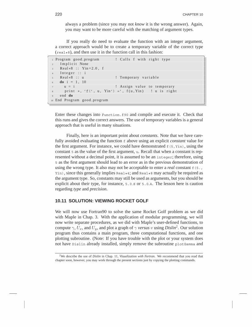
220 CHAPTER 10
always a problem (since you may not know it is the wrong answer). Again,you may want to be more careful with the matching of argument types.
If you really do need to evaluate the function with an integer argument,a correct approach would be to create a temporary variable of the correct type(real*8), and then use it in the function call in this fashion:
1 Program good program ! C a l l s f w i th r i g h t t y p e2 I m p l i c i t None3 Rea l ∗8 : : Yin = 2 . 0 , f4 I n t e g e r : : i5 Rea l ∗8 : : u ! Temporary v a r i a b l e6 do i = 1 , 107 u = i ! Ass ign v a l u e t o t e m p o r a r y8 p r i n t ∗ , ’f(’ , u , Yin’) =’ , f ( u , Yin ) ! u i s r i g h t9 end do
10 End Program good program
Enter these changes into Function.f90 and compile and execute it. Check thatthis runs and gives the correct answers. The use of temporary variables is a generalapproach that is useful in many situations.
Finally, here is an important point about constants. Note that we have care-fully avoided evaluating the function f above using an explicit constant value forthe first argument. For instance, we could have demonstrated f(5,Yin), using theconstant 5 as the value of the first argument, u. Recall that when a constant is rep-resented without a decimal point, it is assumed to be an integer; therefore, using5 as the first argument should lead to an error as in the previous demonstration ofusing the wrong type. It also may not be acceptable to enter a real constant f(5.,Yin), since this generally implies Real*4; and Real*8 may actually be required asthe argument type. So, constants may still be used as arguments, but you should beexplicit about their type, for instance, 5.0 8 or 5.0 4. The lesson here is cautionregarding type and precision.
10.11 SOLUTION: VIEWING ROCKET GOLF
We will now use Fortran90 to solve the same Rocket Golf problem as we didwith Maple in Chap. 3. With the application of modular programming, we willnow write separate procedures, as we did with Maple’s user-defined functions, tocompute γ, Ux, and Uy, and plot a graph of γ versus v using Dislin2. Our solutionprogram thus contains a main program, three computational functions, and oneplotting subroutine. (Note: If you have trouble with the plot or your system doesnot have Dislin already installed, simply remove the subroutine plotGamma and
2We describe the use of Dislin in Chap. 11, Visualization with Fortran. We recommend that you read thatchapter soon, however, you may work through the present sections just by copying the plotting commands.

DATA TYPES, LIMITS, PROCEDURES; ROCKET GOLF 221
its call statement to do the exercises in this section). To determine how round-offerror affects the results, we describe and run the program that solves the problem indouble-precision, and then ask you to modify it so that it solves the same problemin single-precision (we give the results of both, but only the source file for thedouble-precision version).
Listing 10.5 Golf.f90
1 ! Gol f . f90 : The GOLF program wi th DISLIN p l o t2 ! −−−−−−−−−−−−−−−−−−−−−−−−−−−−−−−−−3 Program g o l f d o u b l e4 I m p l i c i t None5 Rea l ∗8 : : Up , Tp , v , t h e t a , T , uxva l , uyva l , u , p h i6 Rea l ∗8 , P a r a m e t e r : : PI = 3.14159265358979323846 87 Rea l ∗8 : : gamma , Ux , Uy8 ! S e t i n i t i a l v a r i a b l e s f o r M i c h e l l e :9 Up = 1 . 0 8 / S q r t ( 3 . 0 8 )
10 Tp = 2 . 6 e7 811 v = 0 . 5 812 t h e t a = 3 0 . 0 8 ∗ PI / 1 8 0 . 0 813 ! C a l l f u n c t i o n s t o g e t v a r i a b l e s f o r Ben :14 T = gamma ( Up ) ∗ Tp15 u x v a l = Ux ( Up , t h e t a , v )16 u y v a l = Uy ( Up , t h e t a , v )17 u = S q r t ( u x v a l ∗∗ 2 + u y v a l ∗∗ 2)18 p h i = Atan2 ( uyval , u x v a l )19 ! D i s p l a y r e s u l t s :20 p r i n t ∗ , ’T =’ , T21 p r i n t ∗ , ’ux =’ , u x v a l22 p r i n t ∗ , ’uy =’ , u y v a l23 p r i n t ∗ , ’u =’ , u24 p r i n t ∗ , ’phi =’ , p h i25 ! P roduce t h e P l o t o f gamma ( v ) vs . v :26 c a l l plotGamma27 End Program g o l f d o u b l e28
29 ! F u n c t i o n gamma ( v ) − t ime d i l a t i o n f u n c t i o n30 Rea l ∗8 F u n c t i o n gamma ( v )31 I m p l i c i t None32 Rea l ∗8 : : v33 gamma = 1 . 0 8 / S q r t ( 1 . 0 8 − v ∗∗ 2)34 End F u n c t i o n gamma35
36 ! F u n c t i o n Ux r e t u r n s x v e l o c i t y37 Rea l ∗8 F u n c t i o n Ux ( Up , t h e t a , v )38 I m p l i c i t None39 Rea l ∗8 : : Up , t h e t a , v , Upx40 Upx = Up ∗ Cos ( t h e t a )41 Ux = ( Upx + v ) / ( 1 . 0 8 + v ∗ Upx )42 End F u n c t i o n Ux43
44 ! F u n c t i o n Uy r e t u r n s y v e l o c i t y

222 CHAPTER 10
45 Rea l ∗8 F u n c t i o n Uy ( Up , t h e t a , v )46 I m p l i c i t None47 Rea l ∗8 : : Up , t h e t a , v , Upx , Upy48 Rea l ∗8 : : gamma49 Upx = Up ∗ Cos ( t h e t a )50 Upy = Up ∗ Sin ( t h e t a )51 Uy = Upy / ( gamma ( v ) ∗ ( 1 . 0 8 + v ∗ Upx ) )52 End F u n c t i o n Uy53
54 ! S u b r o u t i n e t o pe r fo rm t h e p l o t55 S u b r o u t i n e plotGamma56 Use d i s l i n ! R e q u i r e d f o r DISLIN r o u t i n e s57 I m p l i c i t None58 I n t e g e r , P a r a m e t e r : : n=100059 I n t e g e r : : i60 Rea l ∗8 , Dimension ( n ) : : xv , yg61 Rea l ∗8 : : v , gamma62 ! C r e a t e X and Y a r r a y s t o p l o t :63 v = 0 . 064 do i = 1 , n65 xv ( i ) = v66 yg ( i ) = gamma ( v )67 v = v + . 0 0 1 868 end do69 ! C a l l DISLIN p l o t t i n g r o u t i n e s :70 c a l l m e t a f l (’XWIN’ ) ! d e f i n e d i s p l a y f o r m a t71 c a l l d i s i n i ! i n i t i a l i z e D i s l i n72 c a l l t i t l i n (’gamma(v) vs. v’ , 1 ) ! d e f i n e l i n e 1 t i t l e73 c a l l name (’v’ , ’X’ ) ! X a x i s l a b e l74 c a l l name (’gamma(v)’ , ’Y’ ) ! Y a x i s l a b e l75 c a l l g r a f (−0.05 8 , 1 . 0 5 8 , 0 . 8 , . 1 8 , −1. 8 , 2 6 . 8 , 0 . 8 , 5 . 8 )76 c a l l g r i d ( 1 , 1 ) ! a x i s marks and g r i d s77 c a l l t i t l e ! i n s e r t t i t l e78 c a l l c o l o r (’RED’ ) ! c o l o r o f c u r v e79 c a l l c u r v e ( xv , yg , n ) ! draw t h e l i n e80 c a l l d i s f i n ! f i n i s h D i s l i n81 End S u b r o u t i n e plotGamma
Lst. 10.5 shows the program Golf.f90. It creates initial data for the angleand velocity of Michele’s golf ball, and computes the velocities and angles asseen by Ben. If you set the speed of light c equal to a nearly-infinite number, therelativistic effects vanish. Observe that in this example we have placed the mainprogram first in the file, followed by the functions gamma, Ux, and Uy, and then thesubroutine plotGamma. Some programmers prefer the main program to be listedfirst as it shows from the start how the entire program works. This is top-downprogramming. Other programmers prefer defining all the procedures (functionsand subroutines) first before they are called. That is bottom-up programming. TheFortran compiler does not care if you call a procedure before it is defined as longas it is defined somewhere within the source file (or in other modules that are

DATA TYPES, LIMITS, PROCEDURES; ROCKET GOLF 223
Figure 10.3 A plot of the function γ(v) output from the program Golf.f90. Compare to similarplot done with Maple in Chap. 3.
referenced by the Include statement).
Find where the function Uy calls the function gamma. Having one functioncall another is acceptable modular programming practice. Also note that we havekept the main program neat by placing all the plotting commands in the subroutineplotGamma. This keeps the technical details from interfering with our ability tosee the logical flow of the program, and permits us to modify the plotting withoutmessing up the rest of the program. The plot obtained is shown in Fig. 10.3, andlooks much like the Maple plot in Chap. 3.
To create a single-precision version of the program, you will have to convertReal*8’s into Real*4’s and change the 8’s attached to the numerical constants:
10 v = 0.5 411 theta = 30.0 4 * PI/180.0 4
Running this code on a PC with Compaq Fortran, produces the following outputfor the two cases:
/* Golf: Double-Precision */ /* Golf: Single-Precision */T = 31843366.6561813 T = 3.1843368E+07ux = 0.800000000000000 ux = 0.8000000uy = 0.200000000000000 uy = 0.2000000u = 0.824621125123532 u = 0.8246211phi = 0.244978663126864 phi = 0.2449787
This output is the Fortran solution to the first part of the problem, where Michelehits the golf ball forward. Realize that the exact output of these values (format and

224 CHAPTER 10
significant digits) may differ based on machine type, operating system, compiler,etc. Generally, we will see that Fortran is smart enough to realize that its single-precision calculations have 6-7 places of precision, and so prints out just 8 signifi-cant figures (an extra one or two places so you are able to see the imprecision). Incontrast, Fortran prints out 16 or 17 significant figures for double-precision, wherewe expect 15-16 places of precision.
In the second part of the problem, Michele hits the golf ball backwards (atθ = 150). To find a solution here, we have to modify the program. In the double-precision version, we should change the line theta = 30.0 8 * PI / 180.0 8 sothat it reads
theta = 150.0 8 * PI / 180.0 8
After making this modification, the results we obtained when running the programon a PC are the following:
/* Golf: Double-Precision */ /* Golf: Single-Precision */
T = 31843366.6561813 T = 3.1843368E+07 sux = -1.480297366166875E-016 ux = -7.9472862E-08uy = 0.333333333333333 uy = 0.3333333u = 0.33333333333333333 u = 0.3333333phi = 1.57079632679490 phi = 1.570797
Notice where the differences in precision occur between single and double in theseexamples. Also notice the differences between these results here as run on a PCand the results you have produced on your computer system.
When we solve the third part of the problem and look at the x componentof velocity that Ben sees for the backward hit, we find that the double and single-precision calculations give:
ux = -1.4802973661668753E-016 ux = -7.9472862E-08
Assessment
It is honest to say that the single- and double-precision results differ by a factorof 100 million! Yet this is not good computational science. It is better to say thatwithin the precision of the calculation, both calculations agree that the x-velocityis zero, but that it is very hard for floating-point computations to give a result thatis exactly zero.
Another way of interpreting these numbers is to say that the double-precisioncomputation appears to have error in the 16th decimal place while the single-precision computation has an error in the 8th place. This is the respective, ex-pected levels of precision, and so both results are small numbers consistent with

DATA TYPES, LIMITS, PROCEDURES; ROCKET GOLF 225
zero. Since the velocities predicted by the programs are much smaller than the ve-locities used as input, this is a case in which subtractions within the program havecancelled off all of the significant figures in our input numbers, and the outputnumbers are of (very) questionable significance.
10.12 YOUR PROBLEM: MODIFY GOLF.F90
1. Save and print out a copy of Golf.f90 from the CD.2. Draw a box around and label each of the procedures in the program.3. Label where each procedure is called.4. Remove or comment out all the Dislin references and calls. This will elimi-
nate any problems with these routines in case Dislin is not installed on yoursystem. The exercises in this section do not require the plotting components.
5. Copy Golf.f90 into a new file GolfReal.f90. Convert the copy into asingle-precision program.
6. Compile and then execute both programs and compare the results for theoutput (the velocity seen by Ben). We do not expect a large difference forsuch a simple problem, yet it should be noticeable. The difference mightget to be much larger if the calculation were repeated millions of times, asrealistic calculations often are.
7. To keep track of your results, make a table of the form:
UMx UM
y UM θM UBx UB
y UB φB
singledouble
...
where the superscripts M and B are used for Michele and Ben.8. Modify both programs so that θ = 150. This angle corresponds to Michele’s
ball hit to the left at an angle of 30 above the negative x′ axis. Enter yourresults into your table.
9. Compile and execute both programs. Compute the relative error of the double-precision value for ux with respect to the single-precision value for ux:
ureldef=
uD − uS
uS. (10.11)
Also compute the relative error of the single-precision value for ux with re-spect to the double value for ux. Compare the two relative errors. Is relativeerror a useful metric for comparing numbers such as these?
10. Modify the double-precision program so that θ = 0.11. Compile and execute the program. Record results in your table. According
to Ben and equation (10.3), what is the x velocity of Michele’s golf ball?What would the x velocity be if nonrelativistic physics were used? (Thiscorresponds to using these same equations with the speed of light c = ∞, so
226 CHAPTER 10
γ = 1.)12. Modify the double-precision program so that θ = 180, and interpret the
results.13. Determine what Ben sees as the x velocity of the golf ball when the golf ball
is hit 30 below the left horizon, that is, at θ = 210. Compare this to theresult from classical physics.
10.13 KEY WORDS
array binary numbers bitsbytes underflow local variablesmachine precision memory words word lengthmodular programs naming conventions overflowdata type significant digits double-precision
10.14 FURTHER EXERCISES
1. Explain in just a few words what is meant by:a. an integerb. a floating-point numberc. double-precisiond. truncation errore. round-off errorf. a stringg. machine precision and underflowh. number of significant digits and overflow
2. Approximately what are the overflow and underflow limits for double-precisioncomputations in Fortran?
3. Approximately what are the number of significant digits in single and double-precision in Fortran?
4. Imagine that you have just landed that dream job of yours in the local ham-burger joint. Your first assignment is to write a program that figures out whatchange to make if a person buys one item that costs less than a dollar, andpays for it with a dollar bill.a. Compute what change in quarters, dimes, and pennies you would give,
using the minimum number of coins. Hint: Work entirely in integerarithmetic, and define the integers: price, change, quarters, dimes,and pennies. To name an instance, 27 cents would be represented by theinteger 27, and change = 100 - price, quarters = change/25, etc.
b. Modify the program so that it uses floating-point variables and commenton the different results.
5. Write the following numbers in scientific notation so that they reflect thegiven number of significant digits:a. 25.3 to four significant figures.
DATA TYPES, LIMITS, PROCEDURES; ROCKET GOLF 227
b. 0.00005 to two significant figures.c. 1.351 to two significant figures.d. 84000 to three significant figures.
6. Suppose that the floating-point number system on your computer has two-digit mantissas and exponents ranging from -2 to 1. Indicate whether thefollowing expressions each would result in Overflow, Underflow, Roundofferror, or an Exact answer.
a) 20. + 20. b) 50. * 50. c) 20. + 0.01d) 20. * 0.01 e) 0.01 + 0.01 f) 0.01 * 0.01
7. You have encountered a number of examples in which a program was con-structed to contain several functions or subroutines rather than do all of thecomputations within the main function. In reflecting on these examples, doesdividing a program into procedures make ita. longer or shorter?b. harder or easier to understand?c. more or less difficult to debug?d. more or less likely to reuse components?
8. Consider a Fortran program in which the main program uses a functionInteger f(x,y) (where x is Real*8 and y is Integer) that is defined justonce. Indicate whether each of the following is true or false:a. the main program must call f with variables having the names x and y
b. the function f may change the value of f(x, y)c. if the main program calls f with two integer arguments, f will convert the
first one to double-precision.d. the function f returns a double-precision valuee. the variable type returned by f depends upon the arguments given to it.
9. Indicate the values that Fortran would produce for the following expressions:a. 4/2 =b. 4/3 =c. 3/4 =d. 3./4 =e. 4/3. =
10. Explain what the values of a and b are at the end of the following bit of code.Integer :: i = 3, j = 2
Real*8 :: a, b, c = 3
a = 1 + i/j + j/i
b = 1 + c/j + j/c

Chapter Eleven
Visualization with Fortran
11.1 AN OVERVIEW OF DISLIN
We have already seen in Maple how visualizations are helpful in understandingresults and in debugging computations, as well as adding some fun to your work.There are two basic ways to do visualization in Fortran. The traditional, and stilleffective, approach is to run your computation and save the output to a file (easyin Fortran), and then use a separate program such as Gnuplot [Gnuplot] or Grace(AceGr) [Grace] to plot the data as a separate process. When the simulations aretime consuming (“expensive”), or the data sets large, this is often the preferredapproach.
The second approach to data visualization is to do plotting from within yourprogram using Fortran-callable routines. The Fortran language itself does not con-tain universal graphical constructs, as exist in Java. We recommend and demon-strate Dislin [Dislin]. It is powerful, free for many users, appropriate for science,and available for many Fortran compilers. While we find it somewhat harder toinstall and use than PtPlot in Java, it is the best we can find for Fortran. If you havetrouble with it, remember that Gnuplot and AceGr will still serve you well.
The DISLIN data-plotting library was written by Helmut Michels at the MaxPlanck Institute in Lindau, Germany. Its name is an abbreviation for Device-Independent Software LINdau since it is system-independent to a high degree,which allows Fortran programs using Dislin to be ported from one operating sys-tem to another without changes. Dislin consists of subroutines and functions forgraphically displaying data in the form of curves, bar graphs, pie charts, 3-D colorplots, surfaces, contours, and maps. You should reference the Dislin home pageat www.dislin.de for more information. If your system does not have Dislin in-stalled, then you cannot run our example programs. (§11.2 describes how to installDislin).

VISUALIZATION WITH FORTRAN 229
2-D Graphs within Fortran using Dislin
Listing 11.1 EasyDislinPlot.f90
1 ! E a s y D i s l i n P l o t . f90 : Simple p l o t u s i n g D i s l i n2 !−−−−−−−−−−−−−−−−−−−−−−−−−3 Rea l F u n c t i o n f ( x ) ! c o u l d s u b s t i t u t e any t a s k4 Real , i n t e n t ( i n ) : : x5 f = cos ( x )6 End F u n c t i o n f7 !8 Program E a s y D i s l i n P l o t9 Use d i s l i n
10 I m p l i c i t None11 I n t e g e r , p a r a m e t e r : : n=50012 Real , d imens ion ( n ) : : xValues , yValues13 Rea l : : f , f a c t o r , x s t e p14 I n t e g e r : : i15 ! C r e a t e some d a t a f o r t h e X and Y a r r a y s t o p l o t16 f a c t o r = 1 0 . / n17 do i =1 , n , 118 xValues ( i ) = ( i −1) ∗ f a c t o r19 yValues ( i ) = f ( xValues ( i ) )20 end do21 ! D i s l i n p l o t t i n g r o u t i n e s22 c a l l m e t a f l (’XWIN’ ) ! d e f i n e i n t e n d e d d i s p l a y23 c a l l d i s i n i ! d i s l i n i n i t i a l i z e24 c a l l p a g e r a25 c a l l complx26 c a l l a x s p o s ( 4 5 0 , 1 8 0 0 )27 c a l l a x s l e n ( 2 2 0 0 , 1 2 0 0 )28 c a l l name (’x-axis’ ,’X’ )29 c a l l name (’y-axis’ ,’Y’ )30 c a l l l a b d i g (−1 ,’X’ )31 c a l l t i c k s ( 1 0 ,’XY’ )32 c a l l t i t l i n (’DISLIN graphics demonstration with CURVE’ , 1 )33 c a l l t i t l i n (’f(x) = cos(x)’ , 3 )34 x s t e p = xValues ( n ) / 1 0 . ! i n c r e m e n t f o r l a b e l s35 c a l l g r a f ( 0 . , xValues ( n ) , xValues ( 1 ) , x s t e p , −1 . , 1 . , −1 . , . 2 )36 c a l l t i t l e37 c a l l c o l o r (’RED’ )38 c a l l c u r v e ( xValues , yValues , n ) ! c o n n e c t t h e d a t a p o i n t s39 c a l l c o l o r (’FORE’ )40 c a l l dash41 c a l l x a x g i t42 c a l l d i s f i n ! d i s l i n f i n i s h43 End Program E a s y D i s l i n P l o t
The program EasyDislinPlot.f90 in Lst. 11.1 plots cos(x) versus x. We recom-mend that you use this code as a “black box”, that is, without trying to understandany more of it than you have to! We do not expect you to understand every Dislin

230 CHAPTER 11
command without extensive review of documentation. However, here are somebrief explanations that should help you understand much about this program:
• The function f contains a simple function which is to be plotted. You couldeasily place your own function in its place for experimentation. We suggest youtry a few modifications.
• On line 9 is the command use dislin. This permits your program to import theplotting package. It is a requirement in order to use any of the Dislin routines.
• Lines 16 through 20 initialize the variables. Note that the variables xValues andyValues are arrays (discussed later in Chapter 17) with multiple elements to holdthe x and y values to be plotted. The do - end do pair of statements bracket thepopular Fortran do-loop covered in detail in Chapter 12.
• Lines 22 through 42 are the Dislin subroutine calls. Line 22 establishes theintended display format before the other Dislin routines are called into action; line23 and line 42 act as a pair to initialize and then finish the Dislin routines.
• Lines 24 through 27 set up the plotting environment for an A4 page (standardmetric size of 2969 by 2099 pixels - picture elements, or dots). The axspos com-mand places axes on this page with the arguments of the function correspondingto the lower left corner of an axis system and axslen sets the length of the axes.If the calls in this segment of code are omitted, you will be left with the Dislindefault settings, which are quite acceptable.
• name: labels the axes. The first argument is the string name for the axis, thesecond is the internal string name for the axis.
• titlin: defines the title string. Then title builds and inserts the title appropri-ately.
• graf: plots a 2D-axis system with the stated ranges and tick marks.
• color: sets the color of the plotted points and the curves connecting them.
• curve: connects data points with lines (or can plot them with symbols).
• dash: changes the line plotting style from solid to dashed. The xaxgit commandplots only the y = 0 line.

VISUALIZATION WITH FORTRAN 231
Figure 11.1 The Dislin output from the program EasyDislinPlot.f90.
Running the Sample Program
Run the sample program EasyDislinPlot.f90 to see the plot for yourself. Ona PC, once Dislin is installed, simply use the f90link command that is suppliedwith the Dislin package. With its -a option, it is customized to handle the compile,link, and execution of your program (including all needed Dislin libraries). Whenusing this command, do not enter the .f90 extension. Here is the command withthe option you will need:
> f90link -a EasyDislinPlot Compile, link, and run using single-precision
If the double-precision Dislin libraries are required for a program, then you wouldsimply add the -r8 option like this example:
> f90link -a -r8 EasyDislinPlot Use double-precision libraries
Dislin allows for a variety of graphic output capabilities. In our program, weused XWIN to indicate output to a small window on the screen. If we had preferredto create a file containing our plot, then we could have used BMP to create a bit-map file. By default, it would be automatically named DISLIN.BMP; however, by

232 CHAPTER 11
adding the setfil routine, we can establish the filename of our choice. Here is anexample:
call metafl(’BMP’) define bit-map as the output format
call setfil(’my plotfile.bmp’) name the bit-map file
Once created, this file could be printed or saved for future reference. When cre-ating a file to contain a graph image for printing, it is important to note the fore-ground/background contrast. In Dislin, the default image contains a black back-ground and white foreground which looks great on a screen, but is difficult toprint. One might prefer these colors to be reversed. This can easily be done withthe following call placed right after the calls to metafl and setfil:
call scrmod(’REVERS’) reverse foreground/background
These calls that define the output display structure must all be given before initial-izing Dislin with call disini.
The table below lists all the possible output options. Although some mayrequire other routines for full support, this list will provide a good overview of theDislin output capabilities:
Device Output TypeCONS VGA screen (full window)XWIN VGA screen (small window)GKSL A GKSLIN metafile will be createdCGM A CGM metafile will be createdPS A PostScript file will createdEPS An EPS file will createdPDF A PDF file will createdWMF A Windows metafile will be createdHPGL A HPGL file will be createdSVG A SVG file will be createdJAVA A Java applet file will be createdGIF A GIF file will be createdTIFF A TIFF file will be createdPNG A PNG file will be createdPPM A PPM file will be createdBMP A BMP file will be createdIMAG An Image file will be created
Look at the EasyDislinPlot.f90 program to verify what kind of output was in-
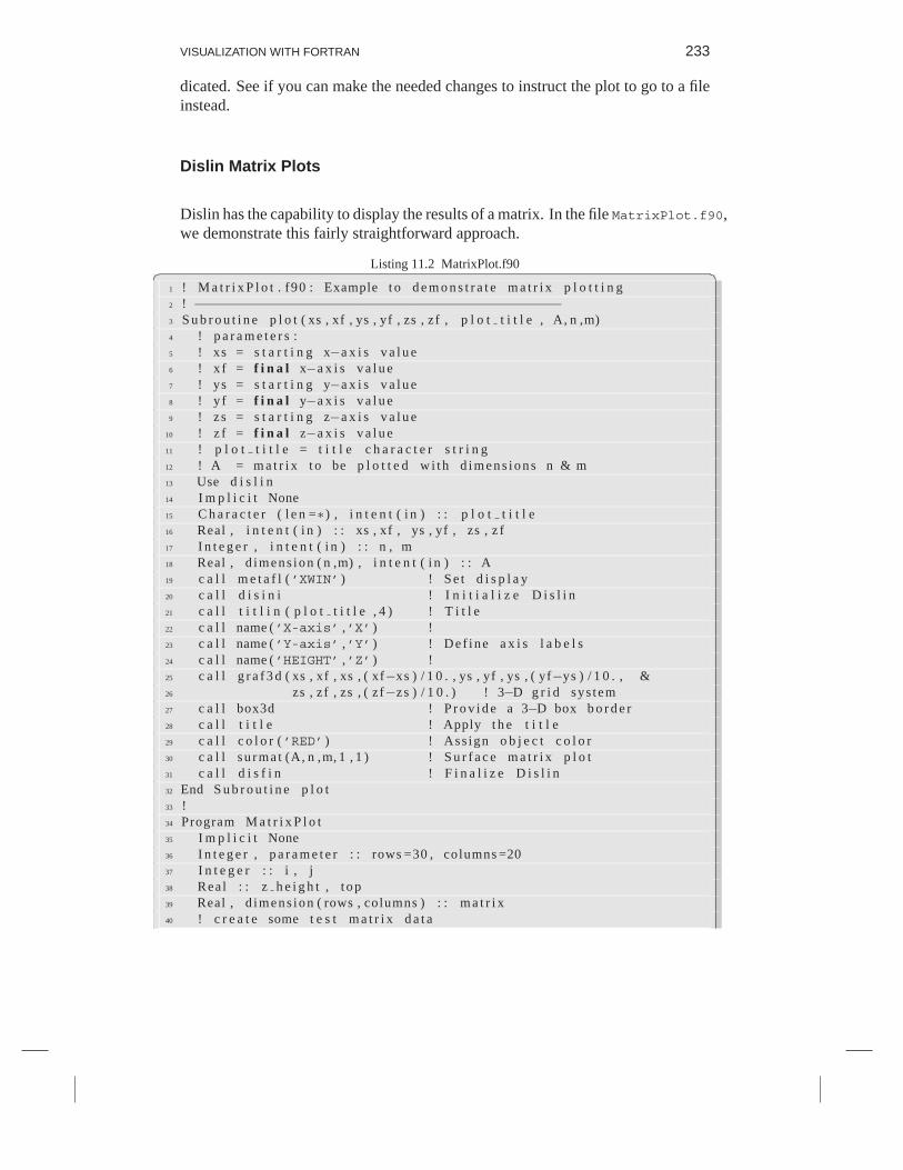
VISUALIZATION WITH FORTRAN 233
dicated. See if you can make the needed changes to instruct the plot to go to a fileinstead.
Dislin Matrix Plots
Dislin has the capability to display the results of a matrix. In the file MatrixPlot.f90,we demonstrate this fairly straightforward approach.
Listing 11.2 MatrixPlot.f90
1 ! M a t r i x P l o t . f90 : Example t o d e m o n s t r a t e m a t r i x p l o t t i n g2 ! −−−−−−−−−−−−−−−−−−−−−−−−−−−−−−−−−−−−−−−−−−−−−−3 S u b r o u t i n e p l o t ( xs , xf , ys , yf , zs , zf , p l o t t i t l e , A, n ,m)4 ! p a r a m e t e r s :5 ! xs = s t a r t i n g x−a x i s v a l u e6 ! x f = f i n a l x−a x i s v a l u e7 ! ys = s t a r t i n g y−a x i s v a l u e8 ! y f = f i n a l y−a x i s v a l u e9 ! z s = s t a r t i n g z−a x i s v a l u e
10 ! z f = f i n a l z−a x i s v a l u e11 ! p l o t t i t l e = t i t l e c h a r a c t e r s t r i n g12 ! A = m a t r i x t o be p l o t t e d w i t h d i m e n s i o n s n & m13 Use d i s l i n14 I m p l i c i t None15 C h a r a c t e r ( l e n =∗) , i n t e n t ( i n ) : : p l o t t i t l e16 Real , i n t e n t ( i n ) : : xs , xf , ys , yf , zs , z f17 I n t e g e r , i n t e n t ( i n ) : : n , m18 Real , d imens ion ( n ,m) , i n t e n t ( i n ) : : A19 c a l l m e t a f l (’XWIN’ ) ! S e t d i s p l a y20 c a l l d i s i n i ! I n i t i a l i z e D i s l i n21 c a l l t i t l i n ( p l o t t i t l e , 4 ) ! T i t l e22 c a l l name (’X-axis’ ,’X’ ) !23 c a l l name (’Y-axis’ ,’Y’ ) ! D e f i n e a x i s l a b e l s24 c a l l name (’HEIGHT’ ,’Z’ ) !25 c a l l g r a f 3 d ( xs , xf , xs , ( xf−xs ) / 1 0 . , ys , yf , ys , ( yf−ys ) / 1 0 . , &26 zs , zf , zs , ( zf−zs ) / 1 0 . ) ! 3−D g r i d sys tem27 c a l l box3d ! P r o v i d e a 3−D box b o r d e r28 c a l l t i t l e ! Apply t h e t i t l e29 c a l l c o l o r (’RED’ ) ! Ass ign o b j e c t c o l o r30 c a l l s u r m a t (A, n ,m, 1 , 1 ) ! S u r f a c e m a t r i x p l o t31 c a l l d i s f i n ! F i n a l i z e D i s l i n32 End S u b r o u t i n e p l o t33 !34 Program M a t r i x P l o t35 I m p l i c i t None36 I n t e g e r , p a r a m e t e r : : rows =30 , columns =2037 I n t e g e r : : i , j38 Rea l : : z h e i g h t , t o p39 Real , d imens ion ( rows , columns ) : : m a t r i x40 ! c r e a t e some t e s t m a t r i x d a t a
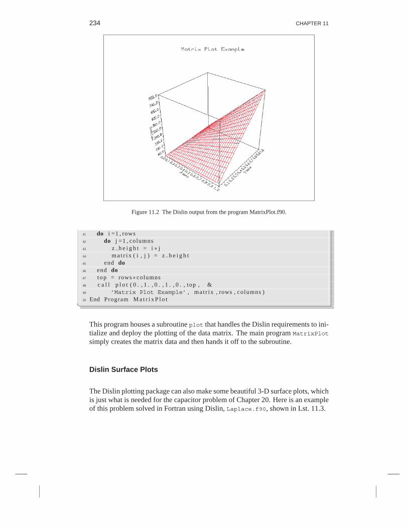
234 CHAPTER 11
Figure 11.2 The Dislin output from the program MatrixPlot.f90.
41 do i =1 , rows42 do j =1 , columns43 z h e i g h t = i ∗ j44 m a t r i x ( i , j ) = z h e i g h t45 end do46 end do47 t o p = rows∗ columns48 c a l l p l o t ( 0 . , 1 . , 0 . , 1 . , 0 . , top , &49 ’Matrix Plot Example’ , ma t r i x , rows , columns )50 End Program M a t r i x P l o t
This program houses a subroutine plot that handles the Dislin requirements to ini-tialize and deploy the plotting of the data matrix. The main program MatrixPlot
simply creates the matrix data and then hands it off to the subroutine.
Dislin Surface Plots
The Dislin plotting package can also make some beautiful 3-D surface plots, whichis just what is needed for the capacitor problem of Chapter 20. Here is an exampleof this problem solved in Fortran using Dislin, Laplace.f90, shown in Lst. 11.3.

VISUALIZATION WITH FORTRAN 235
Listing 11.3 Laplace.f90
1 ! L a p l a c e . f90 : L a p l a c i a n e l e c t r o s t a t i c s on s q u a r e g r i d , P l o t2 ! −−−−−−−−−−−−−−−−−−−−−−−−−−−−−−−−−−−−−−−−−3 S u b r o u t i n e p l o t ( xs , xf , ys , yf , zs , zf , p l o t t i t l e , A, xdim , ydim )4 ! p a r a m e t e r s :5 ! xs = s t a r t i n g x−a x i s v a l u e6 ! x f = f i n a l x−a x i s v a l u e7 ! ys = s t a r t i n g y−a x i s v a l u e8 ! y f = f i n a l y−a x i s v a l u e9 ! z s = s t a r t i n g z−a x i s v a l u e
10 ! z f = f i n a l z−a x i s v a l u e11 ! p l o t t i t l e = t i t l e c h a r a c t e r s t r i n g12 ! A = L a p l a c e m a t r i x o f d imens ion xdim & ydim13 Use d i s l i n14 I m p l i c i t None15 C h a r a c t e r ( l e n =∗) , i n t e n t ( i n ) : : p l o t t i t l e16 Real , i n t e n t ( i n ) : : xs , xf , ys , yf , zs , z f17 I n t e g e r , i n t e n t ( i n ) : : xdim , ydim18 Real , d imens ion ( xdim , ydim ) , i n t e n t ( i n ) : : A19 c a l l m e t a f l (’XWIN’ )20 c a l l d i s i n i21 c a l l name (’X-axis’ ,’X’ )22 c a l l name (’Y-axis’ ,’Y’ )23 c a l l name (’Z-axis’ ,’Z’ )24 c a l l t i t l i n ( p l o t t i t l e , 4 )25 c a l l g r a f 3 d ( xs , xf , xs , ( xf−xs ) / 1 0 . , ys , yf , ys , ( yf−ys ) / 1 0 . , &26 zs , zf , zs , ( zf−zs ) / 1 0 . )27 c a l l box3d28 c a l l t i t l e29 c a l l c o l o r (’GREEN’ )30 c a l l s u r m a t (A, xdim , ydim , 1 , 1 )31 c a l l d i s f i n32 End S u b r o u t i n e p l o t33 !34 S u b r o u t i n e s o l v e (V, tmax , imax ) ! C r e a t e t h e d a t a35 I m p l i c i t None36 I n t e g e r , i n t e n t ( i n ) : : imax , tmax37 Real , i n t e n t ( o u t ) , d imens ion ( imax , imax ) : : V38 I n t e g e r : : i , j , k , r i g h t , l e f t , top , bot tom39 r i g h t = imax / 3 ! r i g h t edge o f t h e c a p a c i t o r40 l e f t = 2∗ imax / 3 ! l e f t edge o f t h e c a p a c i t o r41 t o p = 2∗ imax / 3 ! uppe r c a p a c i t o r42 bo t tom = imax / 3 ! lower c a p a c i t o r43 ! I n i t i a l i z e t h e m a t r i x V t o z e r o44 V=0 .45 ! Boundary c o n d i t i o n s46 V( r i g h t : l e f t , bo t tom ) = −1.047 V( r i g h t : l e f t , t o p ) = 1 . 048 V( 1 , 1 : imax ) = 0 . 049 V( imax , 1 : imax ) = 0 . 050 V( 1 : imax , 1 ) = 0 . 051 V( 1 : imax , imax ) = 0 . 0
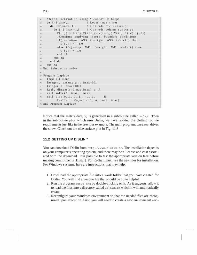
236 CHAPTER 11
52 ! J a c o b i r e l a x a t i o n u s i n g "nested" Do−Loops53 do k =1 , tmax , 1 ! Loops tmax t i m e s54 do i =2 , imax −1 ,1 ! C o n t r o l s row s u b s c r i p t55 do j =2 , imax −1 ,1 ! C o n t r o l s column s u b s c r i p t56 V( i , j ) = 0 . 2 5∗ (V( i +1 , j ) +V( i −1, j ) +V( i , j +1)+V( i , j −1) )57 ! C o n t i n u e a p p l y i n g i n t e r a l boundary c o n d i t i o n s58 i f ( j == bot tom .AND. i >= r i g h t .AND. i <= l e f t ) t h e n59 V( i , j ) = −1.060 e l s e i f ( j == t o p .AND. i >= r i g h t .AND. i <= l e f t ) t h e n61 V( i , j ) = 1 . 062 end i f63 end do64 end do65 end do66 End S u b r o u t i n e s o l v e67 !68 Program L a p l a c e69 I m p l i c i t None70 I n t e g e r , p a r a m e t e r : : imax =10171 I n t e g e r : : tmax =100172 Real , d imens ion ( imax , imax ) : : A73 c a l l s o l v e (A, tmax , imax )74 c a l l p l o t ( 0 . , 1 . , 0 . , 1 . , − 1 . , 1 . , &75 ’Realistic Capacitor’ , A, imax , imax )76 End Program L a p l a c e
Notice that the matrix data, V, is generated in a subroutine called solve. Thenin the subroutine plot which uses Dislin, we have isolated the plotting routinerequirements just like in the previous example. The main program, Laplace, drivesthe show. Check out the nice surface plot in Fig. 11.3
11.2 SETTING UP DISLIN *
You can download Dislin from http://www.dislin.de. The installation dependson your computer’s operating system, and there may be a license and cost associ-ated with the download. It is possible to test the appropriate version free beforemaking commitments [Dislin]. For Redhat linux, use the RPM files for installation.For Windows systems, here are instructions that may help:
1. Download the appropriate file into a work folder that you have created forDislin. You will find a readme file that should be quite helpful.
2. Run the program setup.exe by double-clicking on it. As it suggests, allow itto load the files into a directory called C:\dislin which it will automaticallycreate.
3. Reconfigure your Windows environment so that the needed files are recog-nized upon execution. First, you will need to create a new environment vari-

VISUALIZATION WITH FORTRAN 237
Figure 11.3 The Dislin output from the program Laplace.f90.
able named dislin with C:\dislin as its value. Next, you will need to addC:\dislin\win to your current PATH environment variable (the subdirectory\win contains the Dislin library routines). Both of these actions may be donefrom the My Computer icon on your desktop:a. Right-click on My Computer, then click on Properties, then Advanced,
then Environment Variables. Do NOT change System Variables.b. To create a new Dislin environment variable, click on New, then enter
dislin as the variable name and C:\dislin as the variable value. Thenclick OK.
c. To add the correct Dislin search path to your PATH environment variable,click on PATH inside the box that lists the variables. Now click Edit (notNew). Within the variable value box, click your pointer directly behindthe last search path item, then add a semi-colon and the additional searchpath (with no spaces). This addition should look like ;C:\dislin\win,then click OK.
d. Finally, click OK in the Environment Variables window. Click Apply,then OK in the System Properties box.
4. Now, change directories to C:\dislin and compile dislin.f90 in that di-rectory. It is best to do this from within a DOS window. Once you haveinitiated a DOS window:> cd /d C:\dislin Change to the Dislin directory
> f90 -c dislin.f90 Compile to ensure compatibility

238 CHAPTER 11
Note that the file dislin.mod contains interfaces for all Dislin routines. Itmust be referenced from all procedures that utilize Dislin routines via the com-mand Use dislin at the top of each procedure requiring it.
Compilation and execution of Fortran programs that use Dislin should bestbe performed from a DOS window when running on a PC. As mentioned earlier,the Dislin package supplies a convenient linking command called f90link locatedin the \win subdirectory. Remember that DOS can always find it now because youhave added its search path to your PATH environment variable. This command willcompile, link, and execute (including all needed libraries) in one fell swoop (byusing its -a option). By default, f90link uses the single-precision Dislin libraries.For double-precision, add the -r8 option to reference the double-precision Dislinlibraries. Here are examples again for your reference:
> f90link -a prog Compile, link, run prog.f90 using single
> f90link -a -r8 prog Compile, link, run prog.f90 using double
For other operating systems you may have to download the compressedsource code1 and compile it for their system.
11.3 GNUPLOT BASICS
Gnuplot is a versatile 2-D and 3-D graphing package that makes Cartesian, polar,surface, and contour plots. It is open software, available for free on the Web, andproduces many output formats.
You begin gnuplot with a file of (x y) data points. In Fortran so far, we haveonly demonstrated how to write data and text to the screen. Chapter 13 presentsmore details about various input/output (I/O) capabilities. Briefly, here is a shortcode segment that may help for now:
1 open ( UNIT=1 , FILE=’graph.dat’ ) ! Open f i l e 1 , c a l l i t g raph . d a t2 do i =1 , imax , 13 w r i t e ( UNIT=1 ,∗ ) x ( i ) , y ( i ) ! Wr i t e t o g raph . d a t4 end do5 c l o s e ( UNIT=1) ! C lose f i l e 1
Once you have generated a file of your (x y) data, say, graph.dat, thenyou issue the gnuplot command from a shell or from the Start menu. You then
1If you have never done this before, you may want to do it with a friend. In Windows, you can use WinZip tounzip files. In Unix, you can try double-clicking the file in the file manager, or decompress it from the terminalwith the gunzip or tar -xvf commands.

VISUALIZATION WITH FORTRAN 239
Figure 11.4 A gnuplot graph for three data sets with impulses and lines.
get a new window with the gnuplot prompt gnuplot>.You construct your graphby entering gnuplot commands at the gnuplot prompt or by using the pull-downmenus in the gnuplot window:
> gnuplot // Start gnuplot programTerminal type set to ’x11’ Type of terminal for Unix
gnuplot> The gnuplot prompt
gnuplot> plot "graph.dat" Plot data file graph.dat
In Figure 11.4 we plot a number of graphs on the same plot using several data filesand the command:
gnuplot> plot ’graph.dat’ with impulses, ’2.dat’, ’3.dat’ with lines
The general form of the 2-D plotting command is:
plot ranges function title style , function ...
with points Default. Plot symbol at each pointwith lines Plot lines connecting the pointswith linespoint Plot lines and symbolswith impulses Plot vertical lines from x axis to pointswith dots Plot small dot at each point (scatter plots)
It is necessary to place all file or directory names in single or double quotes and toseparate file names with a comma. Explicit values for the x and y ranges are set

240 CHAPTER 11
Im T(E)
13001400
15001600
-100
-80
-60
-40
-20
0
-30
-15
0
15
30
Re E (MeV)
Im E (Me V)
Figure 11.5 Gnuplot’s surface plot of a scattering amplitude ImT as a function of complex energyE.
with the plot options:
gnuplot> plot [xmin:xmax] [ymin:ymax] "file" Genericgnuplot> plot [-10:10] [-5:30] "graph.dat" Explicit
Printing Plots
Gnuplot supports a number of printers including PostScript ones. The basic methodof printing plots is:
1. Set “terminal type” for your printer.2. Send the plot output to a file.3. Replot figure for new output device.4. Quit Gnuplot (or get out of Gnuplot window).5. Print file.
You could also import the file into a word processor to have it appear in a documentor into a drawing program to fix it up just right. To see what type of printers andother output devices are supported by Gnuplot, enter the set terminal commandwithout any options into a gnu window for a listing of available terminal types.Here is an example of creating a PostScript figure and printing it:

VISUALIZATION WITH FORTRAN 241
gnuplot> set terminal postscript Choose local printer typeTerminal type set to ’postscript’ Gnuplot response
gnuplot> set term postscript eps Another option
gnuplot> set output "plt.ps" Send figure to file
gnuplot> replot Plot again so file is sent
gnuplot> quit Or get out of gnu window
% lp plt.ps Unix print command
Gnuplot Surface (3-D) Plots
The surface (3-D) plot command is splot, and it is used in the same manner asplot—with the obvious extension from (x, y) to (x, y, z). As discussed in Chap-ter 4, a surface, such as that in Figure 11.5, is specified by giving just the z valuesfor successive rows, with different rows separated by blank lines:
-4.043764 Data for 3-D plot. . .
-11.000000
Because there are no explicit x and y values given, Gnuplot labels the x and y axeswith the row and column number. At present Gnuplot does not have the capabilityto rotate 3-D plots interactively. Instead, you adjust your plot with the command:
gnuplot> set view rotx, rotz, scale, scalez
where 0 ≤ rotx ≤ 180o and 0 ≤ rotz ≤ 360o are angles in degrees, and the scalefactors control the size. Any changes made to a plot are made when you redrawthe plot using the replot command.
To see how this all works, here we give a sample Gnuplot session that wewill use in Chapter 20 to plot a 3-D surface from numerical data. Listing 11.3contains the actual code used to output data in the form for a Gnuplot surface plot.
> gnuplot Start gnuplot system from a shell
Then, a special Gnuplot shell starts up with the prompt gnuplot>, and you areready to give gnuplot your subcommands.2
gnuplot> set hidden3d Hide surface whose view is blockedgnuplot> set nohidden3d Show surface though hidden from view
gnuplot> splot ’Laplace.dat’ with lines Surface plot of Laplace.dat with lines
gnuplot> set view 65,45 Set x and y rotation viewing angles
gnuplot> replot See effect of your change
gnuplot> set contour Project contours onto x-y plane
2Under Windows, there is a graphical interface that is friendlier than the gnuplot subcommands. The subcom-mand approach we indicate here is reliable and universal.

242 CHAPTER 11
gnuplot> set cntrparam levels 10 10 contour levels
gnuplot> set terminal PostScript Output in PostScript format for printing
gnuplot> set output "Laplace.ps" Plot output to be sent to file Laplace.ps
gnuplot> splot ’Laplace.dat’ w l Plot again, output to file
gnuplot> set terminal x11 To see output on screen again
gnuplot> set title ’Potential V(x,y) vs x,y’ Title graph
gnuplot> set xlabel ’x Position’ Label x axis
gnuplot> set ylabel ’y Position’ Label y axis
gnuplot> set zlabel ’V(x,y)’; replot Label z axis and replot
gnuplot> help Tell me more
gnuplot> set nosurface Do not draw surface, leave contours
gnuplot> set view 0, 0, 1 Look down directly onto base
gnuplot> replot Draw plot again; may want to write to file
gnuplot> quit Get out of gnuplot
For this sample session, the default output for your graph is your terminalscreen. To print a paper copy of your graph, we recommend first saving it toa file as a PostScript document (suffix .ps), and then printing out that file to aPostScript printer. You create the PostScript file by changing the terminal typeto Postscript, setting the name of the file, and then issuing the subcommandsplot again. This plots the result out to a file. If you want to see plots on yourscreen again, you need to set the terminal type to x11 again (for Unix’s X WindowsSystem), and then plot it again.

Chapter Twelve
Flow Control via Logic; Projectiles
In this chapter, we begin discussing some of the control structures that make pro-gramming so interesting and that make your programs so intelligent. We will haveyou write your own program to simulate projectile motion, a standard problem ofelementary physics. In Chap. 15, Differential Equations with Maple and Fortran;Projectile Motion with Drag, we solve this same problem including air resistance.We start with a review of the kinematic equations that may be scanned for thosefamiliar with it, and then go on to describe program design and control structures.
12.1 PROBLEM: FRICTIONLESS PROJECTILE MOTION
Figure 12.1 shows the trajectory of a projectile fired from a cannon at time t = 0,with initial velocity V0, at an angle θ relative to the horizon. The projectile remainsin the air for a total hang time of T , and hits the ground at a horizontal distance orrange x = R away from the origin.
Problem: write a program to simulate the motion of this projectile. Have it per-form the following steps:
- 6- 4
- 2
0
2
4
6
8
0 5 10 15 20 25 30 35 40 45
Projectile without/with Air Resistance
x
y
θ
Vox
y
Vo
Voy
x
q
Figure 12.1 Left: The trajectory of a projectile fired with initial velocity V0 in the θ direction.The nonparabolic curve includes air resistance. Right: The components of the initialvelocity V0 projected onto the x and y axes.

244 CHAPTER 12
1. store the initial values V0, g, and θ as constants,2. compute the “hang time” T from the equations of kinematics,3. compute the range R and height H from the equations of kinematics,4. compute each position (x, y) of the projectile starting at −T/2 and running
in 100 uniform steps to 3T/2.
12.2 THEORY: KINEMATICS
If we ignore air resistance, a projectile has only the force of gravity acting onit. This force causes the projectile to fall towards the center of the earth with aconstant acceleration g = 9.8m/s2. The resulting solutions to the equations ofmotion are
x(t) = V0xt, y(t) = V0yt− 12gt
2. (12.1)
Here V0x and V0y are the horizontal and vertical components of the initial velocity,and, as we see from Fig. 12.1,
V0x = V0 cos θ, V0y = V0 sin θ. (12.2)
Likewise, the x and y components of the velocity as functions of time are:
vx(t) = V0x, vy(t) = V0y − gt. (12.3)
Although the equations of motion yield x and y as functions of time, they do nottell us the shape of the trajectory. For these simple equations it is easy to derivethat the shape is a parabola. We will, instead, determine the shape by plotting upthe solution, a simpler approach as the equations become more realistic.
We determine the hang time T by observing that at the time of firing t = 0,and landing t = T , the projectile has a height y = 0. If we set y = 0 in (12.1), weobtain an equation for the time at which the height is zero:
y(t) =V0yt− 12gt
2 = 0, ⇒ V0yt = 12gt
2 (12.4)
⇒ T =2V0y
g, (12.5)
where we ignore the t = 0 solution. Once we know T we find the range R as thehorizontal distance x(T ):
R = x(T ) = V0x2V0y
g=
2V 20 sin θ cos θ
g. (12.6)
The projectile reaches its maximum height H at the midpoint of the trajectory attime t = T/2 = V0y/g:
H = y(T
2) =V0y
V0y
g− 1
2g
(V0y
g
)2
(12.7)
⇒ H =V 2
0 sin2 θ
2g. (12.8)

FLOW CONTROL VIA LOGIC; PROJECTILES 245
12.3 COMPUTER SCIENCE: DESIGNING STRUCTURED PROGRAMS
Now that you are into the program construction business, it is a good idea to under-stand not only the grammar of each instruction within the selected programminglanguage, but also the general structure of a well-built code. Books have beenwritten on program design, but then again, it is a good idea not to believe every-thing you read! Yet, as seems to be true in much of life, it is helpful to follow therules until you know better. Once you have truly mastered a subject, you may thenmake new rules. We view programming as a written art that blends elements of sci-ence, mathematics, and computer science into a set of instructions which permitsa computer to accomplish a scientific goal. Good programs should:
• Give the correct answers.• Be clear and easy to read, with the action of each part of the code easy to
identify and analyze.• Document themselves for the sake of programmers (yourself included) who
must improve or expand the code later.• Be easy to use.• Be structured so that it is easy to modify and robust enough to keep giving the
right answers!• Be passed on to others to use and to develop further.
One way to make your programs clearer is to structure them in an organizedfashion. You may have already noticed that sometimes we show our coding exam-ples with indentation, skipped lines, and strategically placed dividers. This is doneto provide visual clues as to the functioning of the different program components.These organized components are the “structures” in structured programming. Al-though the Fortran compiler ignores these visual clues, the human readers are aidedin understanding and modifying the program by having it arranged in a manner thatnot only looks good, but also makes the different parts of the program manifest tothe eye.
The organization of code into clearly organized task components, is knownas structured programming. This method, presented with the visual clues to helphumans easily identify program components, is highly recommended! It is a valu-able approach when dealing with complex tasks involving multiple control struc-tures, especially when some structures are nested within others. The basic idea issimple: blocks of code performing specified tasks should be organized together,and then indented and physically isolated to set them apart. Even though in our ex-amples (in order to conserve printed space) we do not skip as many lines or add asmany comments as we would like, we recommend that you take these extra stepsin your code design as programs grow in complexity.

246 CHAPTER 12
Start
End
Initializeconstants
BasicCalculations
Loop overtim e
Start
End
Initialize g, V0, theta
Calc R, T, step
Loop: t between -T/2 and 3T/2
0< t< T?T F
calcx(t), y(t)
Printvalues
t< 0?T F
Not yet fired
G rounded
Add step to t
Figure 12.2 A flow chart illustrating a possible program to compute projectile motion. On the left,we show the very high-level basic components of the program, while on the right, weshow some of the details of the logic flow structures.
Flow Charts and Pseudocode
In Fig. 12.2 we present a flowchart that illustrates a possible program to computeprojectile motion. A flowchart is not meant to be a detailed description of a pro-gram with all calculations and exact variable names, but rather a graphical aide tohelp visualize its logical flow. As such, it is independent of which computer lan-guage you may choose and is useful for developing and understanding the basicstructure of an overall task. We recommend that you draw some type of flowchartor construct some type of pseudocode every time you write a program. Pseudocodeis like a text version of a flowchart. Here is an example:
1. Store g, V0, and θ2. Calculate R and T3. Calculate uniform step4. Loop 100 times from −T/2 to 3T/2 by step
a. If t < 0, print “not yet fired”b. If t > T , print “grounded”c. If projectile is in the air, calculate and print x(t) and y(t)d. increment t by step
5. End program

FLOW CONTROL VIA LOGIC; PROJECTILES 247
LogicalCom parison ?
T F
then else
action 3
action 1
action 2
actions A actions B
Figure 12.3 Left: Sequential or linear programming. Right: The if-then-else structure, one of severalstructures used to write nonlinear program segments based on logical decisions.
One way of viewing program design is in terms of data flow. Simplisti-cally, your program starts with some initial data (read or created), decides what todo with it, does it, and then outputs the results. Usually boxes in flowcharts likeFig. 12.3 show straight-forward actions, while elongated or angled boxes showdecisions to be made and the related actions that are needed based on those deci-sions. The direction of logical flow of the program is shown by the arrows, withflow moving down, except when arrows redirect it.
For our projectile problem, we need to calculate the position for 100 differ-ent times. The easiest way to do this is to have the same block of code repeated100 times, with only the value of the time, t, changing. Such a structure is called aloop. Like a clock, our example will run for a total time
Ttotal = Tf − Ti =32T − −T
2= 2T, (12.9)
in steps (ticks) of
∆t =2T100
=T
50. (12.10)
Whence, the time increases by ∆t for each repetition of the loop:
t = t + ∆t, (12.11)
with the program using its intelligence to decide what to compute and print de-pending upon the particular value of t.
12.4 FLOW CONTROL VIA LOGIC
One of the most satisfying aspects of programming is getting the computer to dojust what you want. The control of the computer can be direct, as when you havethe computer evaluate functions in a “calculator” mode like we did with Maple, orit can be more subtle, as when you try to make the computer act intelligently and
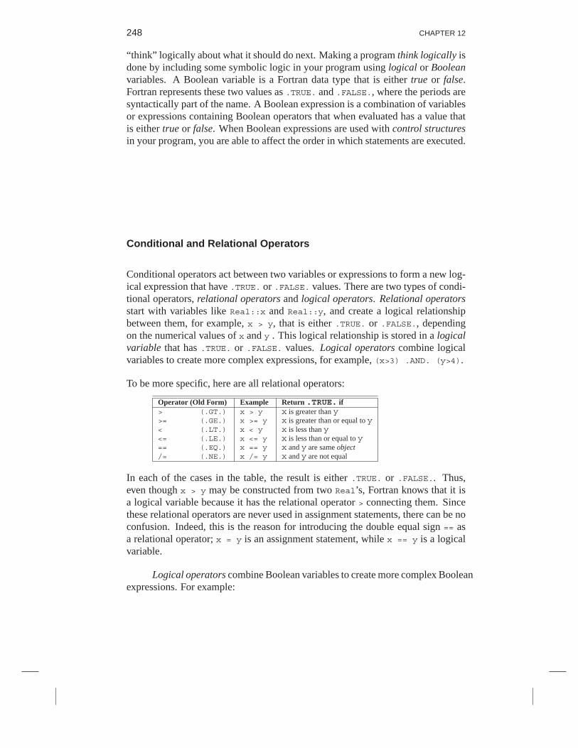
248 CHAPTER 12
“think” logically about what it should do next. Making a program think logically isdone by including some symbolic logic in your program using logical or Booleanvariables. A Boolean variable is a Fortran data type that is either true or false.Fortran represents these two values as .TRUE. and .FALSE., where the periods aresyntactically part of the name. A Boolean expression is a combination of variablesor expressions containing Boolean operators that when evaluated has a value thatis either true or false. When Boolean expressions are used with control structuresin your program, you are able to affect the order in which statements are executed.
Conditional and Relational Operators
Conditional operators act between two variables or expressions to form a new log-ical expression that have .TRUE. or .FALSE. values. There are two types of condi-tional operators, relational operators and logical operators. Relational operatorsstart with variables like Real::x and Real::y, and create a logical relationshipbetween them, for example, x > y, that is either .TRUE. or .FALSE., dependingon the numerical values of x and y . This logical relationship is stored in a logicalvariable that has .TRUE. or .FALSE. values. Logical operators combine logicalvariables to create more complex expressions, for example, (x>3) .AND. (y>4).
To be more specific, here are all relational operators:
Operator (Old Form) Example Return .TRUE. if> (.GT.) x > y x is greater than y>= (.GE.) x >= y x is greater than or equal to y< (.LT.) x < y x is less than y<= (.LE.) x <= y x is less than or equal to y== (.EQ.) x == y x and y are same object/= (.NE.) x /= y x and y are not equal
In each of the cases in the table, the result is either .TRUE. or .FALSE.. Thus,even though x > y may be constructed from two Real’s, Fortran knows that it isa logical variable because it has the relational operator > connecting them. Sincethese relational operators are never used in assignment statements, there can be noconfusion. Indeed, this is the reason for introducing the double equal sign == asa relational operator; x = y is an assignment statement, while x == y is a logicalvariable.
Logical operators combine Boolean variables to create more complex Booleanexpressions. For example:

FLOW CONTROL VIA LOGIC; PROJECTILES 249
Operator Example Name: Return .TRUE. if.AND. x .AND. y Logical and: x and y both true, conditionally evaluates y.OR. x .OR. y Logical or: either x or y true, conditionally evaluates y.NOT. .NOT.x Not: x is false.EQV. x .EQV. y Equivalence: x and y the same.NEQV. x .NEQV. y Nonequivalence: x and y not the same
The basic logic behind logical operators is that if we have a compound statementconstructed from two simpler statements, then the truth table
True Falsetrue and true true and falsetrue or true false and falsetrue or false false or false
not false not true
determines the truth of the compound statement. The logical and is represented by.AND., while .OR. represents the logical or. As a case in point, if x is true, thenx .OR. y is true regardless of y. Believe it or not, what makes the use of logi-cal expressions so powerful is that it is possible to combined the different logicalexpressions to describe the basis for all logical decision.
Exercise: If a is your age in years, w your weight in pounds, and h your heightin inches, construct Boolean expressions that will be true only when the followingstatements are true:
1. you are old enough to obtain a driver’s license but too young to retire, ( (a >
16) & (a < 65)),2. you are not a teenager,3. you are either younger than 20 and less than 150 pounds, or you are older
than 40 and more than 6 feet,4. you are neither old enough to vote, tall enough to hit your head on a five-foot
door frame, nor of the right weight to box in the 132–140 pound division. ♠
Control Structures
The combination of Boolean expressions and control structures permits you toconstruct programs that can handle all possible logical situations. Table 12.1 con-tains a more complete list of control structures, of which we will use only a subset.The type of logic that is possible with these logical expressions is shown in theflowcharts of Figures 12.3-12.4. If you look at both the command in the table, andthe action in the figure together, you should get a good idea how the commandworks.
The left of Fig. 12.3 shows linear or sequential programming in which thestatements are executed in the order in which they are encountered, that is, from

250 CHAPTER 12
Name Example Comment
if-then If ( (x < 3) .AND. (y == 12) ) z = y * x Single line ifmulti-line if-then If ( (x >= 1) .AND. (x <= 9) ) Then If statement
y = 1 Multi-line code blockEndIf End of the If statement
if-then-else If (x <= 0.) Then If statementy = y ** 2 Do this if true
Else Only one Else (“catchall”)y = 3 * y Do this if false
EndIf End of the If statementif-then-else-if If (score >= 90) Then Multi-way if
grade = "A"Else If (score >= 80) Then Any number of Else If’s OK.
grade = "B"Else If (score >= 70) Then Inaccessible if other Else If’s true.
grade = "C"EndIf End of the If statement
do Do count = 1, 100, 1 Initial value, final value, increment<statements> Multi-line code block
End Do End of the Do structuredo-while Do While (x + sin(x) < 0.8) Repeat as long as true
x = x + 0.01 Block of code that is repeatedEnd Do End of the Do structure
select case Select Case (month) Jump to the appropriate caseCase (1)s = "Jan" Do this if month equals 1
Case (6, 7, 8)s = "Summer" Do this if month equals 6, 7 or 8
Case (10:12)s = "Winter" Any month between 10 and 12, inclusive
End Select
Table 12.1 Logical flow control structures in Fortran.
top to bottom. Control structures introduce the possibility that the execution of aprogram may “split” into different paths depending on the values of certain vari-ables, or may repeat certain sections a number of times. If the program does “split,”then the program is no longer sequential.
The if or if-then-else structure, illustrated on the right of Fig. 12.3, is one ofthe most common control structures in programming. It permits your program tomake decisions leading to multiple outcomes, with the decision based on changingsituations. For example: if it is raining before 10 AM, then I will take my umbrella.This structure can be enhanced with the else option: if it is sunny, then I will takemy sunglasses, else I will take my umbrella. The angle-edged box contains alogical expression constructed with the if statement. If the logical expression istrue, then actions A are executed, else actions B are executed.
In the Fortran if-then-else structure illustrated in Fig. 12.3, there are two setsof possible actions; one set is executed if the condition is true and the other setof actions is executed if the condition is false. The syntax requires that actions A

FLOW CONTROL VIA LOGIC; PROJECTILES 251
Loop for anum ber of iterations
actions
Add to counter
Test a logicalcondition
actions,am ong whichcause a changeto the logicalcondition
F
T
Figure 12.4 Left: The Fortran Do-loop iteration. Right: The Fortran Do-while loop uses a generaltest, in contrast to the Do-loop’s iteration count.
consist of a block of statements contained within the paired if and end if state-ments. (When there is only one line of actions needed, however, the then andend if statements are not required; the single action statement simply follows theif logical condition on the same line). If actions B are included as an alternatepath of actions, they must be preceded with the word Else, which occurs on aseparate line of its own right prior to the list of actions B.
Fig. 12.4 illustrates the Fortran do-loop, probably the most popular loopingcontrol structure. The do-loop is used to iterate, that is, repeat a section of code foras long as some condition is true. This is useful for things like summing a seriesor repeating a calculation until the error gets smaller than some fixed amount.Because a counter is used to keep track of the number of iterations, it is also calleda counting loop. The statements that are repeatedly executed are bracketed by theinitial do statement and the closing end do statement.
In the first line of the do structure:
do var = 1, 100, 2 a simple example for discussion
after the keyword do, there is a variable (here, it is named var). It is used to countthe loop iterations; it can be referred to as the counter or the index variable. It isfollowed by three fields separated by commas; these may be constants or variablesor arithmetic expressions, and they may be positive or negative. The first field, 1 inthis case, gives the initial value for the index variable. The second field, 100, givesthe final value for the index. The third field is the increment (or decrement, if it isnegative) for the index variable. For each iteration through the statements withinthe loop, this value is added to the index variable. If the third field is missing, itis assumed to be the positive value 1. The program will continue to repetitivelyexecute all the statements between do and end do until the index variable haspassed the final value. (Note that it is possible to start at 100, decrementing downto 1 using a change value of -1).
do var = 100, 1, -1

252 CHAPTER 12
The iteration of a do-loop ends when the index (or counter) has passed thefinal value. However, if the final condition is already met before any actions aretaken, then the statements inside the do-loop will never be executed. In eithercase, if iteration has ended, or never executed, the program moves on to the firstexecutable statement after the end do statement.
These few ways to incorporate logic into programs are sufficient for theproblem at hand. Nevertheless, there are other commands that use a somewhat dif-ferent approach in controlling the flow of your program, and we shall now discusssome. Consider again the right of Fig. 12.3 illustrating the if-then-else structure.We see in Table 12.1 that the else part of this control structure can have an if-thenstructure following it to form an if-then-else-if structure. What’s more, there canbe any number of else if statements included to handle any number of specialcases. For the example in the table, we may add more else if statements to assigngrades of A+, A-, B+, etc..
The Do-While construct, shown on the right of Fig. 12.4, is similar to the do-loop, and can serve a similar function. It repeats the statements between do while
and end do until the stated logical condition is .False.. The problem is thatwithout a fixed number of iterations, the loop may never end if the programmer hasmade an error (infinite loop). It is literally up to the programmer to decide upon agood test for a general condition, and to be certain that the general condition willeventually be false so that the do while loop ends. However, it’s perfectly legal tostart with the logical condition .FALSE., in which case the loop is never executed.
It is common to have the counter index variable (var in our example, butany variable name is acceptable) in a do loop be an integer, yet this is not required.A real variable may be used, and it may be given a real initial value, terminationvalue, and increment value. You may also use either an integer or real variable in alogical expression within a do while loop to determine if it is time to end the loop.Be that as it may, be warned that round-off error makes it rather meaningless todemand true equality between two floating-point numbers, or between a real andan integer. For example, the following loop may never complete:
Real*8 :: x = 0.do while (x /= 100.) Comparison may never be satisfiedx = x + 1. Increment
end do
To make sure that the loop will eventually stop, it is better to use the greater-thanand less-than operators <=, <, >=, > when comparing values as part of the logicalexpression for a do while loop. The == and /= operators should be avoided, unlessthere is a good reason to use them, such as when one wishes to determine if asequence has converged exactly to a given value.
Listing 12.1 Select.f90

FLOW CONTROL VIA LOGIC; PROJECTILES 253
1 ! S e l e c t . f90 : D e m o n s t r a t e s t h e use o f S e l e c t Case c o n t r o ls t r u c t u r e
2 !−−−−−−−−−−−−−−−−−−−−−−−−−−−−−−−−−−−−−−−−−−−−−−−−−−−−−−3 Program s e l e c t e x a m p l e4 I m p l i c i t None5 I n t e g e r : : wake , month6 do month = 12 , 0 , −1 ! Loop f o r 13 months7 p r i n t ∗ , ’Month is ’ , month ! P r i n t c u r r e n t month8 s e l e c t case ( month ) ! Choose case v i a month9 case ( 0 ) ! Here f o r month 0
10 p r i n t ∗ ,’ Last year’11 case ( 1 ) ! Here f o r month 112 wake = 913 p r i n t ∗ ,’ January, wake =’ , wake14 case ( 2 ) ! Here f o r month 215 wake = 716 p r i n t ∗ ,’ February, wake =’ , wake17 case ( 4 ) ! Here f o r month 418 wake = 619 p r i n t ∗ ,’ April, wake =’ , wake20 case d e f a u l t ! Here o t h e r c a s e s21 wake = 822 end s e l e c t ! End S e l e c t23 end do ! End Do24 End Program s e l e c t e x a m p l e
Select Case
The Select Case structure is a neat way to execute different blocks of code depend-ing upon the value of an integer or string variable. While this also can be accom-plished with a series of if-then statements, as we said, Select Case is neater. Asan instance, consider the program Select.f90 in Lst. 12.1 that we use to programour clock radio.
Compile and execute Select.f90 to see what the output looks like. Notethat the do-loop on line 6 counts down on the value of month from 12 to 0. Oncewithin the loop, there is a printout on line 7 that outputs the value of month. Nextwithin the do-loop is the select case on line 8 controlled by the value of month.If month = 0, 1, 2, 4, execution will jump to the lines starting with case followedby the corresponding value of month. If the value of month is not one of thesecases, then execution jumps to the case default on line 20. When executionjumps to one of the listed cases, the value of the wakeup time variable wake is setand printed. Once execution is completed within a case set of actions, the programjumps to the next statement after the end select statement.

254 CHAPTER 12
Select Case Exercise:1. Add in wakeup times and printouts for three more months.2. See what happens if you leave off the case default component on lines 20-21.3. See what happens if the order of the Case statements is changed. ♠
12.5 IMPLEMENTATION: PROJECTILE.F90
1. Before you write your program, write down the equations to be solved. Handthis in with your assignment, and refer to it while working on the program.
2. Create a flow chart, or some pseudocode, that shows the logic of your pro-gram. Think of the logic flow as the path that converts the initial data to theprinted results. Hand this in, too.
3. Using the program limits.f90 from Chapter 10 as an initial program frame-work, open it with your editor and then save it as projectile.f90, a new filein the appropriate directory/folder for this week.
4. Modify projectile.f90 to compute and print T , H and R in a line beforethe do-loop. (In other words, strip out the ”limit” tasks and insert the ”pro-jectile” tasks).
5. Modify the do-loop so that it loops over i = 1 to 100.6. Declare a variable t2, the time variable that changes as the projectile flies
through the air. Within the do-loop, calculate t2 by the formula t2 = −T/2+2 ∗ T ∗ (i/100.).
7. Inside the do-loop, use if statements to decide if the projectile has not yetbeen fired, if it’s in the air, or if it has already hit the ground.
8. Have your program print “not yet fired” or “grounded” as appropriate. Oth-erwise, print explicit values for x(t2) and y(t2).
9. Have your program make a plot of the particle trajectory. Your instructor mayhave to help you determine the available plotting packages for your system.
12.6 SOLUTION: PROJECTILE TRAJECTORIES
1. Run your program for a variety of initial conditions, that is, for your choiceof different values for V0 and θ. Try some for which you know the expectedanswer (like θ = 0 and θ = π/2).
2. Check that the range R increases as the initial velocity V0 increases in mag-nitude, and as the elevation θ increases from 0 to π/4.
3. Check that the range R = 0, but that the hang time T = 0, for θ = 90o (thiscorresponds to shooting the cannon straight up in the air, not the most cleverthing to do).
4. Check that the y values never exceed the maximum height H .

FLOW CONTROL VIA LOGIC; PROJECTILES 255
12.7 KEY WORDS
air resistance Boolean variable select case conditional opcontrol structure counting loop decrement op flowchartif-then-else increment op flow control do whileiteration linear program logical operators operatorpseudocode relational op repetition structure structured program
12.8 SUPPLEMENTARY EXERCISES
1. Take the program Limits.f90 from Chapter 10 that uses a do-loop to deter-mine machine precision, and make a copy of it.a. Compile and run Limits.f90 as a check that it is still running, and to get
some output for comparison.b. Modify the do-loop so that the counter is a double precision variable. You
should get all the same results.c. Change the do-loop to a do while loop that accomplishes the same task.
(Hint: while (1.0 + epsilon m /= 1.0) will repeat the loop until thereis no difference between the stored values of 1.0 + epsilon m and 1.0.)
d. Include an if-then construct in the loop so that the program prints only oneline of output, and that is for the first time that 1.0 + epsilon m = 1.0.
e. Include an if-then-else construct in the loop so that the program prints themessage “not there yet” if 1.0 + epsilon m /= 1.0, and then the usualone and epsilon m the first time that 1.0 + epsilon m = 1.0.
2. If a is your age in years, w is your weight in pounds, and h is your heightin inches, construct Boolean expressions that will be true only when the fol-lowing conditions are met:a. you are old enough to obtain a driver’s license and you do not weigh 1000
pounds.b. you are not a teenager.c. you are either younger than 20 and less than 150 pounds, or older than 40
and greater than 6 feet.d. you are neither old enough to vote, tall enough to hit your head on a
five-foot door frame, nor the right weight to box in the 132–140 pounddivision.
3. Let: A be your age, Y the number of years you have been in college, and Dthe number of dollars you have in the bank. Construct Boolean expressionsthat will be true when the following conditions are met:a. you are a millionaire but you are not a senior.b. you are either too young to vote or you are not a freshman.c. you are either younger than 20 and broke, or older than 90 and have more
than $100,000.d. you are 16 years old and your number of years in college is greater than
the number of dollars you have in the bank.
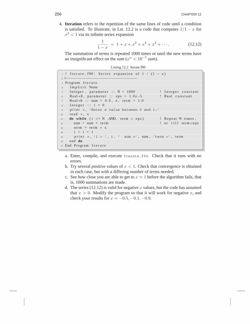
256 CHAPTER 12
4. Iteration refers to the repetition of the same lines of code until a conditionis satisfied. To illustrate, in Lst. 12.2 is a code that computes 1/1− x forx2 < 1 via its infinite series expansion
11− x
= 1 + x + x2 + x3 + x4 + · · · . (12.12)
The summation of terms is repeated 1000 times or until the new terms havean insignificant effect on the sum (xn < 10−7 sum).
Listing 12.2 Iterate.f90
1 ! I t e r a t e . f90 : S e r i e s e x p a n s i o n o f 1 / (1 − x )2 !−−−−−−−−−−−−−−−−−−−−−−−−−−−−−−−−3 Program I t e r a t e4 I m p l i c i t None5 I n t e g e r , p a r a m e t e r : : N = 1000 ! I n t e g e r c o n s t a n t6 Rea l ∗8 , p a r a m e t e r : : eps = 1 . 0 e−5 ! Rea l c o n s t a n t7 Rea l ∗8 : : sum = 0 . 0 , x , t e rm = 1 . 08 I n t e g e r : : i = 09 p r i n t ∗ , ’Enter a value between 0 and 1:’
10 r e a d ∗ , x11 do whi l e ( i <= N .AND. te rm > eps ) ! Repea t N t imes ,12 sum = sum + term ! o r t i l l term<eps13 t e rm = term ∗ x14 i = i + 115 p r i n t ∗ , ’i = ’ , i , ’ sum =’ , sum , ’term =’ , t e rm16 end do17 End Program I t e r a t e
a. Enter, compile, and execute Iterate.f90. Check that it runs with noerrors.
b. Try several positive values of x < 1. Check that convergence is obtainedin each case, but with a differing number of terms needed.
c. See how close you are able to get to x 1 before the algorithm fails, thatis, 1000 summations are made.
d. The series (12.12) is valid for negative x values, but the code has assumedthat x > 0. Modify the program so that it will work for negative x, andcheck your results for x = −0.5,−0.1,−0.9.

Chapter Thirteen
Fortran Input and Output
The Fortran programmer is blessed with a variety of powerful and high-level I/Ostatements and formats to use. “High-level” here means that you do not have toworry about all the details, while “format” means that Fortran will produce a formfor your output so that it looks just the way you want, including alignment. Herein Lst. 13.1 is a sample code that contains a number of I/O statements:
Listing 13.1 FortranIO.f90
1 ! F o r t r a n I O . f90 : I n p u t / Outpu t example2 ! −−−−−−−−−−−−−−−−−−−−3 Program demo IO4 I m p l i c i t None5 Rea l : : PI , r , power , a r e a6 C h a r a c t e r (LEN=50) : : name7 PI = 3.141592653589798 w r i t e (∗ , ∗ ) ’Enter your name: ’ ! Outpu t s t r i n g9 r e a d (∗ , ∗ ) name ! I n p u t s t r i n g
10 name = t r i m ( name )11 w r i t e (∗ , ∗ ) ’Ciao, ’ , name ! Outpu t s t r i n g + v a r i a b l e12 w r i t e (∗ , ∗ ) ’Now, enter radius & power: ’13 r e a d (∗ ,∗ ) r , power ! I n p u t 2 v a r i a b l e s14 a r e a = PI ∗ ( r ∗∗power ) ! Compute a r e a15 w r i t e (∗ , 100) name , r , a r ea , power ! Wr i t e t o s c r e e n16 w r i t e (∗ , 200) name , r , a r ea , power ! Wr i t e t o s c r e e n17 open ( 1 , FILE=’data.dat’ ,STATUS=’REPLACE’ ) ! Open f i l e18 w r i t e ( 1 , 100) name , r , a r e a ! Wr i t e t o f i l e + f o r m a t19 c l o s e ( 1 , STATUS=’KEEP’ ) ! C lose f i l e20 w r i t e (∗ , ∗ ) ’See data.dat for the answer in the file.’21 s t o p22 100 Format ( / , ’Example 1:’ , / ,’Hello,’ , T10 , A8 , / , 5X, &23 ’The area of a circle with radius ’ , F12 . 6 , &24 2X, ’is ’ ,2 E12 . 3 / / )25 200 Format (’Example 2: ’ , a8 , 1X, 3G12 . 3 , / / )26 End Program demo IO
A typical session of running f90 produces the screen output:

258 CHAPTER 13
Enter your name:LorenCiao, LorenNow, enter radius & power:10 2
Example 1: Hello, LorenThe area of a circle with radius 10.000000 is 0.314E+03 0.200E+01
Example 2: Loren 10.0 314. 2.00
See data.dat for the answer in the file.
13.1 BASIC I/O
The simplest input and output in Fortran is writing to the computer screen andreading from the keyboard. This is the default, and is thus called standard I/O. Forexample, on lines 8 and 11 of FortranIO.f90 we have
8. write(*, *) ’Enter your name: ’11. write(*, *) ’Ciao, ’, name
The write command is used for output. It takes two arguments in parenthesis, thefirst indicating where to write (what device), and the second indicating what formatto use when writing. Both these commands above do the simplest thing, which isto use an asterisk * in place of an explicit argument. The first * indicates that noUNIT is being specified on which to write, so Fortran will use the default outputdevice (the computer screen). The second * indicates that no format statement isbeing specified (free format), and so Fortran will decide what format to use basedon the types and values of the variables being output.
Usually a comma-separated list of variables follows the parenthesis in I/Ocommands. On line 8, the quotes indicate an explicit string to be output, ratherthan the name of a variable. On line 11, the first element in the list is again anexplicit string, while the second element is name, a character variable.
Input can be just as simple. For example:
13. read(*,*) r, power
Here, two variables previously declared as real are read in, with the variablenames separated by a comma. Notice that since we have used the default * again,we do not specify things like where the decimal point occurs in the input or howmany spaces are used to separate the values on input. In fact, the two values to beinput can be on one line separated by spaces, or commas, or tabs, or even on sepa-rate lines. The default input device is the computer keyboard, and Fortran figuresout the format on its own from the data it finds.

FORTRAN INPUT AND OUTPUT 259
13.2 FORMATTED OUTPUT
When you want to specify the exact format of input or output, then the second *in the read and write statements above should be replaced by a numbered label.This label is included as part of the format statement in your program, making itpossible for any I/O statements in the program to reference and use it. The internalpart of the Format statement defines your desired I/O layout:
15 write(*, 100) name, r, area, power16 write(*, 200) name, r, area, power
22 100 Format(/,’Example 1:’,/,’Hello,’,T10, A8,/,5X, &
23 ’The area of a circle with radius ’, F12.6, &
24 2X, ’is ’,2E12.3//)
25 200 Format(’Example 2: ’,a8, 1X, 3G12.3,//)
Here the write statements on lines 15 and 16 output identical variables but withdifferent format statements (as indicated by the labels 100 and 200). The formatstatements and their labels are found on lines 22 and 25, but may be placed any-where in the program since they are just used for reference (not executable actioncommands). To keep format statements out of the way of the program’s logicalflow, they are often placed at the end of the code, right before the End Program
statement. We see that format statement 100 produces verbose output, while 200
contains minimal output, but with variables in a slightly different output format.
Some of the basic input and output types in Fortran are:
Type Meaning Type MeaningA CHARACTER (Alphanumeric) data E REAL (Exponential) dataT Tab to a column F REAL (Fixed decimal point) dataG General format I INTEGER dataX Blank space L Logical
Here A denotes alphanumeric (strings), E denotes a real number in the exponentialform, F produces a fixed decimal point, G is a general format that switches betweenF to E depending upon the size of the number, X represents a blank space, L is forlogical (.TRUE., .FALSE.) variables, and T is used to tab to some column.
These format types take modifiers to control the total number of digits (width) usedfor the I/O, how many digits appear after the decimal point, and whether some fieldis repeated:

260 CHAPTER 13
Example MeaningA8 8 character alphnumeric
E12.3 exponential of width 12 digits, with 3 after decimalF12.6 fixed point of width 12 with 6 after decimalG12.3 general of width 12 digits, with 3 after decimal
I4 Integer of width 4 digits2X 2 blank spaces
3G12.3 3 general fields of width 12 with 3 digits after the decimal
So now if we go back and look at 100 format on line 22, we see a bunchof format instructions separated by commas. The slash / tells the computer toskip a line, ’Example 1:’ and ’Hello,’ are strings that get output exactly asentered. Accordingly, T10 causes the line to tab to column 10 and A8 prints outan alphanumeric variable (your name) using 8 places. The / causes the output toskip to another new line, which is then indented by 5 spaces as indicated by the 5X.The long string enclosed in quotes is printed on that new line. After that, F12.6outputs a real value in a field 12 places wide, with 6 digits after the decimal point.Then there is another string followed by two real values printed as 2E12.3, thatis, as 12-character wide fields with 3 digits after the decimal points, and with anexponent. Notice how the formatting of these same variables gets changed when200 Format is used!
13.3 FILE I/O
Fortran has many options for file I/O that give you the flexibility needed for var-ious tasks. However, since file I/O deals with the hardware and operating systemof your local computer, it is important to check out various versions of these com-mands to see which ones work best on your local system.
File I/O can be either free-form or formatted (the second argument to theread and write commands). In order to write to a file or read from a file, youmust specify a UNIT number associated with the file (this goes in place of the first* in the I/O commands parentheses). In FortranIO.f90, we associated UNIT 1with the filename data.dat, in the same directory as the executing program, via
17 open(1, FILE=’data.dat’, STATUS=’REPLACE’)
where REPLACE indicates that it is OK to replace an older version of the file. Thisstatement may appear anywhere in your program, although we prefer to put OPENstatements at the top of the program, so they do not get in the way of the logic andso it is easy to see which UNITs and filenames are being used. The actual writingto the file is done with the write command:
18 write(1, 100) name, r, area
which uses the same Format statement that we used for screen output. You may

FORTRAN INPUT AND OUTPUT 261
construct any format to meet your needs, but you do not want to spend a lot oftime engineering a beautiful output for a one-time run. Since format statementsare referenced by their numerical labels, several I/O statements can use the sameformat.
Although not strictly needed in many cases, it is always good housekeepingto close any files that you may have opened:
19 close(1, STATUS=’KEEP’)
This releases resources for other tasks, as well as protects the file you have writtenin case of crashes.

Chapter Fourteen
Numerical Integration and Nested Loops;
Energy Usage
In this chapter we explore how computers evaluate integrals numerically. We lookat the same energy problem solved with Maple or Mathematica in Chap. 6, wherenumerical integration also had to be used. This chapter provides a fundamentaltechnique for computational science and a better understanding of calculus. Youalso gain experience with nested loops and plotting.
14.1 PROBLEM (SAME AS CHAPTER 6): POWER AND ENERGY
In Chapter 6 we modeled the electrical power use P (t) over time by some simplefunctions. For example,
Model 3: P3(t) =(
4 +t
365+ 1
2 sinπt
91
)(2 + e− sin 2πt
), (14.1)
where the power is in GW (109 watts) and the time t is in days (the top curve inFigure 14.1). Your problem is to determine the total energy used over 1000 days(approximately three years) by evaluating the integral
E(100) =∫ 100
0P3(t)dt, (14.2)
for Model 3, the one that cannot be done analytically.
The highly oscillatory patterns in Figure 14.1 make (14.2) a challenging in-tegral to evaluate (as demonstrated by the quite different answers obtain by casualapplication of Maple and Mathematica). Consequently, we want you to comparethe results from the two different integration rules (trapezoid and Simpson), and tosee if the value for the integral converges as we improve the approximations. Thereare fancier integration rules, but we leave those to the references [Press 94, CP 05].

NUMERICAL INTEGRATION AND NESTED LOOPS; ENERGY USAGE 263
2x10
Model 1Model 2Model 3
0
2
4
6
8
10
12
14
16
18
20
22
24
-0.2 0.0 0.2 0.4 0.6 0.8 1.0 1.2 1.4 1.6 1.8 2.0 2.2 2.4 2.6 2.8 3.0 3.2 3.4 3.6 3.8 4.0
Power in GW vs time in days, (1 on bottom, 3 on top)
t
Power
Figure 14.1 The three models of power consumption. Time t is in 100 days and power is in Gi-gaWatts.
14.2 ALGORITHMS: TRAPEZOID AND SIMPSON’S RULES
Consider Figure 14.2 showing an arbitrary function f(x) in the interval a ≤ x ≤ b.The definite integral of this function,
I =∫ b
af(x)dx, (14.3)
is equal to the area under the curve. A traditional way to measure this area is toplot the integrand on a piece of graph paper and add up the number of little boxeslying below the curve. Seeing that boxes are “quadrilaterals,” numerical integra-tion is also called numerical quadrature, even when it gets beyond the explicitbox-counting stage.
Numerical-integration techniques usually break the total interval up intosmall columns, as also shown in Figure 14.2, and then use different approxima-tions to determine the area of each column. When the areas of all the columnsare added together, we obtain an approximation for the integral as a weighted sumover the integrand f(x) evaluated at points within the integration region:
I =∫ b
af(x)dx
N∑i=1
f(xi)wi. (14.4)

264 CHAPTER 14
Figure 14.2 Left: Straight-line sections used for the trapezoid rule. An individual trapezoid witharea h
2[f(xi) + f(xi+1)] is highlighted. Right: Parabolas used in Simpson’s rule (a
single parabola is fit to each pair of consecutive intervals.
Here the xis are integration points and the wis are integration weights. This is ahandy way to program up an integration algorithm, since we need only change thespecific values for wi (and maybe xi) for different rules.
As the number of integration points N is made progressively larger (nar-rower columns used), the sum in (14.4) should become a progressively better ap-proximation to the integral. However, if too many points are used, then round-offerror tends to accumulate and the approximation stops converging to the exact an-swer. Consequently, the best integration rules are those which obtain the desiredlevel of precision with the least number of points.
Trapezoid Rule
The trapezoid rule is the simplest integration algorithm. As shown on the left ofFigure 14.2, we divide the area under f(x) into a series of columns each of widthh, and form trapezoids by approximating the integrand f(x) by a straight line con-necting the endpoints of each interval. In this case the integral is approximatelyequal to the sum of the areas of the columns.1 The approximation gets progres-sively better as the widths of the trapezoids are made progressively smaller, andthe integrand is better approximated by a straight line within the interval.
1An alternative way of viewing the trapezoid rule is as forming a series of rectangles with horizontal tops, theheight of each rectangle being (fi + fi+1)/2. If we use fi as the height, then we have a version of the trapezoidrule known as Euler’s rule.

NUMERICAL INTEGRATION AND NESTED LOOPS; ENERGY USAGE 265
We first deduce an equation that gives the x value for each integration point.If we evaluate the function at N points, then we have N − 1 columns (it takes twopoints to define one column) covering the range b–a. It follows then that the widthof each interval in Figure 14.2 is
h =b− a
N − 1, (14.5)
and the discrete x values. They are thus enumerated with the subscript i:
xi = a + (i− 1)h, i = 1, N. (14.6)
To calculate the area of each trapezoid in Figure 14.2, we look at the isolatedcolumn i. The area of this one trapezoid is its width times its average height:∫ xi+h
xi
f(x)dx 12h[f(xi) + f(xi+1)], (14.7)
which is the same area one gets if each column is considered as a rectangle withthe top passing through the midpoint of the slanted top. The total area in theintegration region from a to b is the sum of the areas of all the columns:∫ b
af(x)dx h
2f(x1) + hf(x2) + . . . hf(xN−1) +
h
2f(xN ). (14.8)
Observe that because each internal point gets counted twice, it gets weighted by h,whereas the endpoints get counted just once and so are weighted by only h/2. Interms of the notation of our standard integration rule (14.4), the points and weightsfor the trapezoid rule are:
xi = a + (i− 1)h, wi =[h
2, h, . . . , h,
h
2
], i = 1, N. (14.9)
Listing 14.1 Trap.f90
1 ! Trap . f90 : T r a p e z o i d i n t e g r a t i o n2 !−−−−−−−−−−−−−−−−3 Program t r a p4 I m p l i c i t None5 I n t e g e r : : N, i6 Rea l : : A, B , sum , h , w, t7 w r i t e (∗ ,∗ ) "Enter initial and final t values:"8 r e a d (∗ ,∗ ) A, B9 w r i t e (∗ ,∗ ) "Enter number of integration points:"
10 r e a d (∗ ,∗ ) N11 h = (B − A) / ( N − 1)12 sum = 0 .13 do i =1 , N, 114 t = A + ( i −1)∗h15 i f ( i ==1 .OR. i ==N) t h e n16 w = h / 2 .17 e l s e

266 CHAPTER 14
18 w = h19 end i f20 sum = sum + w∗ t ∗∗221 end do22 w r i t e (∗ ,∗ ) ’The sum is ’ , sum23 End Program t r a p
14.3 IMPLEMENTATION: TRAP.F90
In Lst. 14.1 we present a simple Fortran program Trap.f90 that uses the trapezoidrule to evaluate the integral of
∫ BA t2dt. The function t2 to be integrated is written
directly into the program on line 20. Notice that the calculation of the sum overintervals is accomplished within a do-loop. See §10.10 if you prefer the integrandt2 to be a separate function.
1. Compile and run Trap.f90.2. Modify it to determine the energy usage
∫ 1000 P3(t)dt for Model 3.
3. Use a plotting program to produce a plot of Model 3’s P (t) for 100 days, insteps of 10 days.
4. Make a crude graphical estimate (∼ 25% accuracy) of the area under yourP3(t) vs. t curve. Use 10-day column widths, and count the number of boxesin each column (count fractionally filled boxes as full if they are more thanhalf full), or calculate the area of each trapezoid. Make your boxes big sothat you do not have too much work to do, and make sure you have the rightunits (energy=GW-days) for your choice of boxes.
5. Compare the answer for the integral from your program using 10 day widthswith that found from your graph. Do they agree within measurement error?
Implementation with Nested Loops
Our approximation to the area under a curve as the sum of columns with straightor rounded tops should get more accurate as we increase the number of columnsN-1. However, if we make N too large, then round-off error accumulates to thepoint where increasing N further leads to a less accurate answer. To get a feel forthe level of accuracy of our numerical integration technique, we want to increaseN and determine in what decimal place the answer changes. If the answer changesin, say, the fourth decimal place, then we would expect the answer to be good to atleast three places.
Modify a copy of Trap.f90 so that it prints out the value of the integral andthe value for eight values in the range 25 ≤ N ≤ 200. Rather than running the

NUMERICAL INTEGRATION AND NESTED LOOPS; ENERGY USAGE 267
program eight times (increasing the value of N for each run), make the computerdo this for you; modify the program so that it loops over eight values of N:
1 do N = 25 , 200 , 25 ! Ou te r loop i n c r e a s e s N2 · · ·3 do i = 1 , N, 1 ! I n n e r loop sums ove r columns4 · · ·5 end do6 end do
The procedure outlined in this code fragment uses nested loops, that is, one do-loopcontained within another do-loop. Study how for each value of the total numberof points N, everything within the outer loop gets repeated, and this includes theinner-loop’s i-summation over the areas of each column. Consequently, it is im-portant to check that the program re-initializes the value of variables used in theinner loop, in particular, h and sum. If you look at line 11 of Trap.f90, you willnotice that the column width h varies with the number of integration points usedN. Because of that, we need to begin the new outer do-loop before line 11. Next,notice that the summation over column areas is ended by the end do on line 21.As a consequence, we need to end the outer loop incrementing N after line 21.
Improved Method: Simpson’s Rule
Simpson’s rule for integration will also give us an algorithm of the form (14.4),but with different weights than the trapezoid rule. The integration range is againdivided into equal-width columns, with the points given by (14.6). Now, as weshow on the right of Figure 14.2, we approximate f(x) at the top of every twocolumns as a parabola:
f(x) = αx2 + βx + γ. (14.10)
This is a better than using a straight line. With each parabola containing threeunknown parameters, α, β, and γ, we need three values of f(x) to determine them.We do that by having one parabola pass through the tops of two adjacent columns.Whereas the determination of these constants requires some algebra, the idea issimple. What is important is that because parabolas are being fit to successivepairs of columns, Simpson’s rule requires an odd number of integration points Nso that there will be an even number of columns.
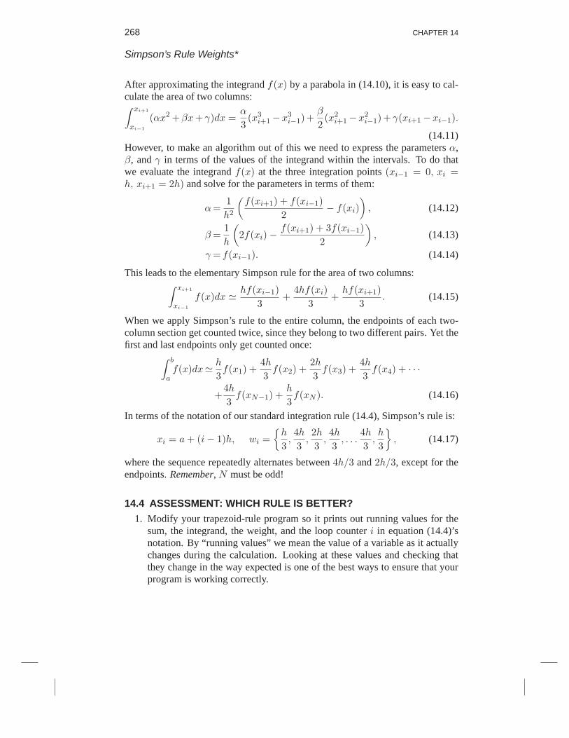
268 CHAPTER 14
Simpson’s Rule Weights*
After approximating the integrand f(x) by a parabola in (14.10), it is easy to cal-culate the area of two columns:∫ xi+1
xi−1
(αx2 +βx+ γ)dx =α
3(x3i+1−x3
i−1)+β
2(x2i+1−x2
i−1)+ γ(xi+1−xi−1).
(14.11)However, to make an algorithm out of this we need to express the parameters α,β, and γ in terms of the values of the integrand within the intervals. To do thatwe evaluate the integrand f(x) at the three integration points (xi−1 = 0, xi =h, xi+1 = 2h) and solve for the parameters in terms of them:
α=1h2
(f(xi+1) + f(xi−1)
2− f(xi)
), (14.12)
β =1h
(2f(xi)−
f(xi+1) + 3f(xi−1)2
), (14.13)
γ = f(xi−1). (14.14)
This leads to the elementary Simpson rule for the area of two columns:∫ xi+1
xi−1
f(x)dx hf(xi−1)3
+4hf(xi)
3+
hf(xi+1)3
. (14.15)
When we apply Simpson’s rule to the entire column, the endpoints of each two-column section get counted twice, since they belong to two different pairs. Yet thefirst and last endpoints only get counted once:∫ b
af(x)dx h
3f(x1) +
4h3f(x2) +
2h3f(x3) +
4h3f(x4) + · · ·
+4h3f(xN−1) +
h
3f(xN ). (14.16)
In terms of the notation of our standard integration rule (14.4), Simpson’s rule is:
xi = a + (i− 1)h, wi =h
3,4h3,2h3,4h3, . . .
4h3,h
3
, (14.17)
where the sequence repeatedly alternates between 4h/3 and 2h/3, except for theendpoints. Remember, N must be odd!
14.4 ASSESSMENT: WHICH RULE IS BETTER?1. Modify your trapezoid-rule program so it prints out running values for the
sum, the integrand, the weight, and the loop counter i in equation (14.4)’snotation. By “running values” we mean the value of a variable as it actuallychanges during the calculation. Looking at these values and checking thatthey change in the way expected is one of the best ways to ensure that yourprogram is working correctly.

NUMERICAL INTEGRATION AND NESTED LOOPS; ENERGY USAGE 269
Figure 14.3 Energy consumption as a function of time for model 1 computed with Maple.
2. Modify a copy of your program so it evaluates the integral using Simpson’srule. Make the program smart enough to use only an odd number of pointsfor Simpson’s rule. Hint: You test if an integer j is even by testing if 2 *(j/2) = j or if j % 2 = 0. The first test takes advantage of the fact thatinteger arithmetic rounds down, while the second test uses a Java method todetermine if the remainder is 0 after division by 2.
3. The numerical approximation for integration should improve as the numberof points N increases. Make a table or plot showing the level of accuracyobtained for the integral for various numbers of points:
N-1 I (trapezoid) I (Simpson)8 - -...
512 - -
4. Make a plot of the energy consumption versus time, like that in Figure 14.3,only here for Model 3. How does that compare to the Maple results?
14.5 KEY WORDS AND CONCEPTS
integration integration points integration weights modular programsnested loops quadrature Simpson’s rule trapezoid rule
1. Explain succinctly the difference between the trapezoid and Simpson rules.2. Is a parabola or a straight line a better approximation for a function?
14.6 SUPPLEMENTARY EXERCISES
1. You are given nonrepeated weights of 1, 2, 4, 8, 16, and 32 kg. Your bossclaims that you should be able to use these six weights to weigh any rice sackweighing an integer number of kilograms between 1 and 63. For instance,

270 CHAPTER 14
63 = 1 + 2 + 4 + 8 + 16 + 32. Write a program to check if the claim is true.The program should write the sack weight and the weights used.
2. As a more challenging version of the above problem, imagine that you aregiven a sack of rice of undermined integer weight less than 64 kg. Write aprogram that determines the sack’s weight and the individual weights youused to determine it.
3. The Chinese scholar Sun Tsu in the year 400 BCE found solutions to theproblem:
find an integer such that if divided by 3 the residue is 2, if dividedby 5 the residue is 3, and if divided by 7 the residue is 2.
Write a program that finds the numbers less that 500 that satisfy these threeconditions.
(These three problems come via courtesy of M. Paez.)
Chapter Fifteen
Differential Equations with Maple and Fortran;
Projectile Motion with Drag*
In this chapter we solve for projectile motion with drag by solving simultane-ous, second-order ordinary differential equations (ODEs) using both Fortran andMaple. This is a fairly realistic problem that is often missing from undergraduateeducation, but whose solution looks familiar to students. The ODE solver usedin our Fortran program is simple, useful for other problems as well, and providessome insight into numerical differentiation. The Maple solution, however, gets tobe surprisingly involved at times due to the equations being both second-order andcoupled, and having a solution that cannot be plotted simply. A comparison of thetwo approaches is quite educational. We have marked this chapter as optional, inpart because there are no new materials that are used elsewhere, and in part be-cause some students may not yet be familiar with differential equations. Howeverthe subject matter is important for many fields, and it does provide a good balanceto the solution of a partial differential equation studied in Chapter 20.
15.1 PROBLEM: PROJECTILE MOTION WITH DRAG
We want to determine if the inclusion of air resistance in projectile motion leadsto trajectories that are much steeper at their ends than their beginnings (golf ballsthat appear to drop out of the sky). We saw in Chapter 12, “Flow Control viaLogic,” that frictionless projectile trajectories are parabolas, symmetric about theirmidpoints, and so do not describe balls dropping out of the sky.
In Figure 12.1 we showed trajectories of a projectile fired from a cannonwithout friction (solid curve) as well as one with air resistance or drag included(dashed curve). The projectile is fired at time t = 0 with velocity V0 at an angleθ relative to the horizon. It remains in the air for a total or hang time t = T andhits the ground a horizontal distance or range x = R away from the origin, withall these quantities apparently changing if air resistance is included. The problemsolution requires us to write a program that predicts or simulates these differenttrajectories for a given set of initial conditions.
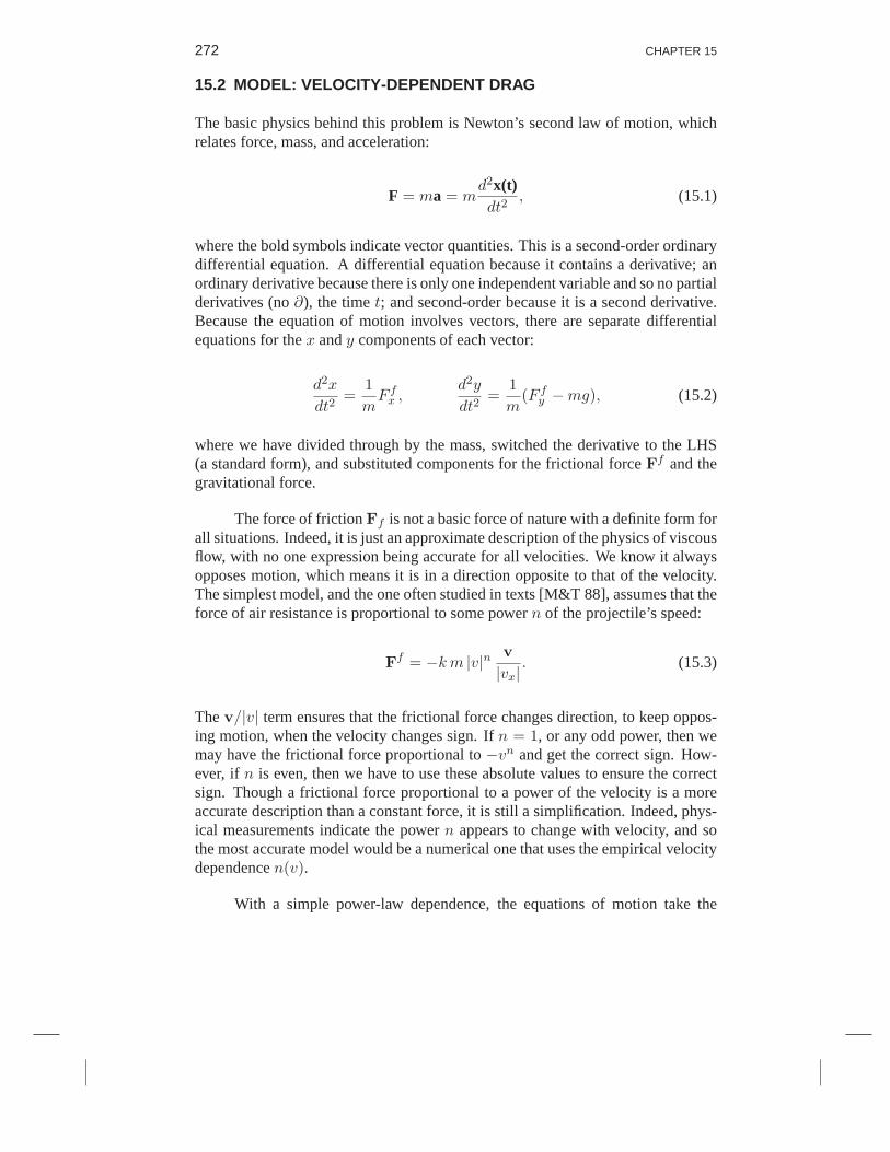
272 CHAPTER 15
15.2 MODEL: VELOCITY-DEPENDENT DRAG
The basic physics behind this problem is Newton’s second law of motion, whichrelates force, mass, and acceleration:
F = ma = md2x(t)dt2
, (15.1)
where the bold symbols indicate vector quantities. This is a second-order ordinarydifferential equation. A differential equation because it contains a derivative; anordinary derivative because there is only one independent variable and so no partialderivatives (no ∂), the time t; and second-order because it is a second derivative.Because the equation of motion involves vectors, there are separate differentialequations for the x and y components of each vector:
d2x
dt2=
1mF fx ,
d2y
dt2=
1m
(F fy −mg), (15.2)
where we have divided through by the mass, switched the derivative to the LHS(a standard form), and substituted components for the frictional force Ff and thegravitational force.
The force of friction Ff is not a basic force of nature with a definite form forall situations. Indeed, it is just an approximate description of the physics of viscousflow, with no one expression being accurate for all velocities. We know it alwaysopposes motion, which means it is in a direction opposite to that of the velocity.The simplest model, and the one often studied in texts [M&T 88], assumes that theforce of air resistance is proportional to some power n of the projectile’s speed:
Ff = −km |v|n v|vx|
. (15.3)
The v/|v| term ensures that the frictional force changes direction, to keep oppos-ing motion, when the velocity changes sign. If n = 1, or any odd power, then wemay have the frictional force proportional to −vn and get the correct sign. How-ever, if n is even, then we have to use these absolute values to ensure the correctsign. Though a frictional force proportional to a power of the velocity is a moreaccurate description than a constant force, it is still a simplification. Indeed, phys-ical measurements indicate the power n appears to change with velocity, and sothe most accurate model would be a numerical one that uses the empirical velocitydependence n(v).
With a simple power-law dependence, the equations of motion take the

DIFFERENTIAL EQUATIONS WITH MAPLE AND FORTRAN; PROJECTILE MOTION WITH DRAG*273
form:1
d2x
dt2= −k vnx
vx|vx|
,d2y
dt2= −g − k vny
vy|vy|
. (15.4)
We shall consider three values for n, each of which represents a different model forthe air resistance: (1) n = 1 for low velocities; (2) n = 3
2 , for medium velocities;and (3) n = 2 for high velocities. For comparison, we will compare these solutionswith air resistance to the analytic results for the frictionless case:
x(t) = v0,xt, y(t) = v0,yt−12gt2, (15.5)
vx(t) = vx,0, vy(t) = vy,0 − gt. (15.6)
15.3 ALGORITHM: NUMERICAL DIFFERENTIATION
In Chapter 5, “Solving Equations, Differentiation,” we used Maple to explore theaccuracy of numerical differentiation. We now apply those techniques in the For-tran solution of differential equations. Most calculus courses start off with thedefinition of the derivative as:
df(x)dx
def= limh→0
f(x + h)− f(x)h
. (15.7)
It is a challenge to apply this definition on a computer, because its finite wordlength causes the numerator to fluctuate between 0 and round-off error as the de-nominator approaches zero. A simple and effective solution is to make h small butnot zero:
df(x)dx
f(x + h)− f(x)h
. (15.8)
Equation (15.8), known as the forward-difference rule, is not the most accurateapproximation [CP 05], but it will suffice.
15.4 MATH: SOLVING DIFFERENTIAL EQUATIONS
When air resistance is present, the force on the projectile depends upon the valueof the velocity, which means that the acceleration is not constant. This makes ananalytic solution to the differential equation difficult, but it is not a challenge toa numerical solution. The trick is to figure out an approximation that takes thesolution at the initial time 0 and advances it a small amount ∆t. Because ∆t issmall, it is not hard to find an approximate solution. One then takes the solutionso found and uses it as the new “initial conditions” to provide the solution at time2∆t. The process is continued until the solution at the desired time is found. With[x(t = 0), y(t = 0)] and [vx(t = 0), vy(t = 0)] as the initial conditions, we have
1For more realistic models used for friction, these equations may become coupled, e.g., because (V 2)x =(Vx)2. For simplicity, we ignore the coupling of the equations, although the technique for the numerical solutionremains unchanged.

274 CHAPTER 15
all the information we need to start the solution and will keep it going as long aswe like.
The simplest algorithm for solving differential equations is a variation ofEuler’s rule. It is based on the fact that for a sufficiently short time interval ∆t,we may assume that the acceleration is constant and use the equations for constantacceleration from elementary physics to advance the velocity and position for ashort time from t to t + ∆t:
x(t+∆t) x(t)+ vx∆t+12ax(∆t)2, vx(t+∆t) vx(t)+ax(t)∆t. (15.9)
Here ax(t) is the variable acceleration at time t. Likewise, there are similar equa-tions for y and vy. To make the algorithm simpler, we assume that ∆t is so smallthat the terms quadratic in ∆t are negligible with respect to the terms linear in ∆t:
x(t + ∆t) x(t) + vx∆t, vx(t + ∆t) vx(t) + ax(t)∆t. (15.10)
This means that as long as we keep the time step ∆t small, we may ignore theacceleration term in (15.9). The acceleration still affects the solution via (15.10),but it does so by changing the velocity, which, in turn, changes the position. Forthis simple method to work, we must choose small values of ∆t. As a rule ofthumb, if the physical system under study has a characteristic time or period ofT , then we would start with ∆t T/100 and then see the effect of decreasingit. A higher-order technique might require fewer steps but use more complicatedformulas.
As our example, we take the simple n = 1 law for air resistance:
d2x
dt2= −kvx,
d2y
dt2= −g − kvy. (15.11)
The terms on the right-hand sides of these equations are the accelerations we needfor the algorithm. The algorithm starts with the given initial position (the origin)and the velocities vx,0, vy,0, and then steps through many time steps. We label thetime steps with the index i = 1 . . . N . For each time step, the position and velocitywill be updated according to the algorithm:
xi+1 = xi + vix ∆t, yi+1 = yix + viy ∆t, (15.12)
vi+1x = vix − k vx ∆t, vi+1
y = viy − k vy ∆t− g∆t. (15.13)
The acceleration due to gravity enters only for the y component of velocity, sincegravity acts only in the y direction. And as we have said, the forces act by directlychanging the velocity, but change the position only indirectly through the changesin velocity.

DIFFERENTIAL EQUATIONS WITH MAPLE AND FORTRAN; PROJECTILE MOTION WITH DRAG*275
Implementation: ProjectileAir.f90
The implementation of the algorithm is given in the code ProjectileAir.f90
shown in Listing 15.1. The program ProjectileAir.f90 contains:
1. a main program that sets initial parameters and directs the computation; and2. a buildPlot subroutine that solves the equations of motion analytically and
numerically and plots each result using the Dislin package.
Examine how the Dislin package is imported with the Use dislin command online 4. On lines 54 and 55 we set the values for the constants, and then initialize thecomputation by calling buildPlot on line 56. The calculation does the frictionlessand with-friction computations simultaneously, with the analytic calculation onlines 21 and 22, and the numeric calculations on lines 27-28. The Dislin plottingroutines are called on lines 32-49, and should give a plot looking like the trajectoryin Figure 12.1.
15.5 ASSESSMENT: BALLS FALLING OUT OF THE SKY?
1. Compile and run ProjectileAir.f90 and check that you get a plot similarto that in Figure 12.1. If your program is not plotting, and your system hasDislin loaded, then you may need to review some of the materials on usingDislin in Chapter 11, “Visualization with Fortran.”
2. In general, it is not be possible to compare analytic and numerical results torealistic problems, because analytic expressions do not exist. However, wedo know the analytic expressions (15.5) for the frictionless case, and we mayturn friction off in our numerical algorithm and then compare the two. This isnot a guarantee that we have handled friction correctly, yet it is a guaranteethat we have something wrong if the comparison fails. Add some lines ofcode to ProjectileAir.f90 that calls the buildPlot procedure a secondtime, this time with the friction coefficient k = 0.
3. We have deliberately given you a program in which the total number of timesteps N is rather small, and, inversely, the time step dt is rather large. Conse-quently, the results from the given program will be of low precision. Repeatthe calculation with ever-increasing values for N, until you cannot tell thedifference on the plot between the numeric and the analytic results for fric-tionless flight.
4. Once the results look good to you, determine the level of precision of the cal-culation by comparing the actual numbers for the analytic and the numericalcalculations. If necessary, increase N until the relative difference is less than1%. Use this value of N for future computations.
5. Add lines to the program so that it prints out and plots up the components ofthe velocity as a function of time.
6. Study your plots of the velocity components versus time and draw a line on

276 CHAPTER 15
Listing 15.1 ProjectileAir.f90
1 ! P r o j e c t i l e A i r . f90 : P r o j e c t i l e Program u s i n g D i s l i n2 ! −−−−−−−−−−−−−−−−−−−−−−−−−−−−−−−−3 S u b r o u t i n e b u i l d P l o t ( Npts , x0 , y0 , v0 , t h e t a , k )4 Use d i s l i n5 I m p l i c i t None6 I n t e g e r , i n t e n t ( i n ) : : Npts7 Rea l ∗8 , i n t e n t ( i n ) : : x0 , y0 , v0 , t h e t a , k8 Rea l ∗8 : : d t , g , vx , vy , xmax , ymax , t9 Rea l ∗8 , d imens ion ( Npts ) : : aXValues , aYValues , nXValues ,
nYValues10 I n t e g e r : : i11 t = 0 .12 g = 9 . 8 113 d t = 2∗v0∗ s i n ( t h e t a ) / ( Npts∗g )14 vx = v0∗ cos ( t h e t a )15 vy = v0∗ s i n ( t h e t a )16 nXValues ( 1 ) = x017 nYValues ( 1 ) = y018 do i =1 , Npts , 119 t = ( i −1)∗ d t20 ! A n a l y t i c21 aXValues ( i ) = x0+v0∗ cos ( t h e t a ) ∗ t22 aYValues ( i ) = y0+v0∗ s i n ( t h e t a ) ∗ t−g∗ t ∗ t / 2 .23 i f ( i >=2) t h e n24 vx = vx−k∗vx∗ d t25 vy = vy−g∗dt−k∗vy∗ d t26 ! Numberic27 nXValues ( i ) = nXValues ( i −1) + vx∗ d t28 nYValues ( i ) = nYValues ( i −1) + vy∗ d t29 end i f30 end do31 ! D i s l i n p l o t t i n g r o u t i n e s32 c a l l m e t a f l (’XWIN’ )33 c a l l d i s i n i34 c a l l name (’x-axis’ ,’X’ )35 c a l l name (’y-axis’ ,’Y’ )36 c a l l l a b d i g (−1 ,’X’ )37 c a l l t i c k s ( 1 0 ,’XY’ )38 c a l l t i t l i n (’ Analytic (green) vs Numerical’ , 1 )39 xmax = 2 .∗ v0∗∗2∗ cos ( t h e t a ) ∗ s i n ( t h e t a ) / g40 ymax = ( v0∗ s i n ( t h e t a ) ) ∗ ∗ 2 / ( 2 . ∗ g )41 c a l l g r a f ( x0 , x0+xmax , x0 , xmax / 1 0 . , y0 , y0+ymax , y0 , ymax / 1 0 . )42 c a l l t i t l e ( )43 c a l l c o l o r (’RED’ )44 c a l l c u r v e ( aXValues , aYValues , Npts )45 c a l l c o l o r (’GREEN’ )46 c a l l c u r v e ( nXValues , nYValues , Npts )47 c a l l c o l o r (’FORE’ )48 c a l l dash49 c a l l d i s f i n50 End S u b r o u t i n e b u i l d P l o t51 !52 Program p r o j e c t i l e A i r53 I m p l i c i t None54 ! Set−up a l l needed p a r a m e t e r s55 I n t e g e r : : Npts = 20056 Rea l ∗8 : : x0 = 0 . , y0 = 0 . , v0 = 2 0 . , t h e t a = 3 . 1 4 1 5 9 2 6 5 3 5 8 9 7 9 / 4 . , k =0 .2557 c a l l b u i l d P l o t ( Npts , x0 , y0 , v0 , t h e t a , k )58 End Program p r o j e c t i l e A i r

DIFFERENTIAL EQUATIONS WITH MAPLE AND FORTRAN; PROJECTILE MOTION WITH DRAG*277
them that appears to be the terminal velocity for each.7. Print out several plots showing the effect of air resistance for different initial
angles θ. For each, determine the value of R, T , and H , and compare thethree with the corresponding values for frictionless flight. All three shoulddecrease.
8. We know that for frictionless flight, the maximum range R occurs for θ =45o, and that there is the same range for trajectories with θ or 90o − θ (forexample, for 30o and 60o). Investigate how both these statements changewhen drag is included. In other words, if you want to hit your golf ball witha maximum range, should you hit it at an angle that is greater than or lessthan 45o?
9. Investigate and describe how the range R varies with initial velocity v0 fora fixed value of θ. Explain the results you obtain (does it go further, forexample?).
10. Up until this point, you have looked at results for the model of friction(15.3) with n = 1. This corresponds to a low-velocity model. Mod-ify ProjectileAir.f90 to investigate n = 2, (high-velocity model) andn = 3/2 (medium-velocity model). To make a realistic comparison, adjustthe value of k for the latter two cases such that the initial force of friction,kV n
0 , is the same for all three cases.
Improved Algorithm: Verlet*
In developing the Euler integration algorithm (15.10), we ignored the direct affectof the acceleration on the position, as is present in (15.9). We now want to modifythe algorithm so that it includes the acceleration term directly in the solution forx(t+ ∆t). An approach that is nearly as simple as Euler yet appears to work verywell is called the Verlet algorithm. It uses second-order terms for xn, but onlyfirst-order ones for vn:
xn+1 = xn+vn∆t+12an(∆t)2, vn+1 = vn+
12(an+1+an)∆t. (15.14)
We see that while the algorithm for the velocity is only first-order in ∆t, it makesup for this somewhat by using the average acceleration over the time interval andnot just its value at the beginning of the interval. The only problem with thismethod is that it is not fully self-contained; to determine vn+1 you first have to usethe Euler method to obtain an+1.
Exercise: Implement the Verlet algorithm and compare the number of stepsneeded to obtain the three-place precision with both the Euler and Verlet meth-ods. (The better algorithm should use fewer steps.) ♠

278 CHAPTER 15
15.6 MAPLE: DIFFERENTIAL-EQUATION TOOLS
Maple is competent at finding solutions to most any differential equation that yougive it. It many cases it can find an analytic solution with no help from you, whilein other cases you may have to give it some hints based on your understanding ofthe mathematics of your equation. If all else fails, or if all you want is a plot of thesolution, ask Maple to solve the differential equation numerically.
In this section we solve the projectile-with-drag problem in Maple. Becausewe have already done this with Fortran, it affords you the opportunity to comparethe two approaches to the same problem. You should decide for yourself; we findthe Fortran solution easier and faster.
Warning: Although the commands we have given here appear to work properlyon various versions of Maple, we have noted that the order in which Maple returnsthe solution changes with different versions. To cite an instance, [y(t), x(t)] in onecase and [x(t), y(t)] in another. Consequently, you may have to reverse the orderof some of the arguments in the plotting commands given below.
We start by repeating the differential equations for projectile motion in auniform gravitational field with no friction, and their solution:
d2
dt2x(t) = 0,
d2
dt2y(t) = −g, (15.15)
x(t) = vo, x t, y(t) = −g t2 + vo, y t. (15.16)
where we have assumed x(0) = y(0) = 0, and used the symbols vo, x and vo, y todenote the x and y components of the initial velocity v0. We start by solving theseequations with Maple and seeing if we get these same solutions. To start simply,first we solve for just the y motion, and then for the simultaneous x and y motions.Then we add in air resistance. This careful approach to a final solution is standardin scientific problem solving.
To keep from repeatedly entering complicated expressions, we give ourequations names and enter the names rather than long expressions. We write ourdifferential equations using the diff command, and later show how to do it withthe D operator (see Chapter 5 for our discussion of derivatives). Yet even if diff isused for the equations, D must be used for the initial conditions.
There are various ways to enter differential equations, and we demonstrateseveral of them (all of which give the same answer of course). We use the variablesdiff eq and diff eq2 for two different representations of the equation for the ycomponent of a projectile’s motion, and solve each with the dsolve command:
> restart; with(DEtools): # Initialize> Vy := diff(y(t), t); # Vy = expression for velocity
DIFFERENTIAL EQUATIONS WITH MAPLE AND FORTRAN; PROJECTILE MOTION WITH DRAG*279
Vy :=d
dty(t)
> diff eq := diff(Vy, t) = - g; diff eq := diff(diff(y(t),t),t) = - g;> diff eq := diff(y(t), t, t) = - g; diff eq := diff(y(t), t$2) = - g;
> diff eq := diff(y(t), t$2) + g; # Multiple forms, same result
diff eq :=d2
dt2y(t) = −g
Two simpler ways of entering the same differential equation is with the D operator:
> diff eq2 := (D2)(y)(t) = -g; diff eq2 := D(D(y))(t) = -g; # With D
diff eq2 := (D(2))(y)(t) = −g
We solve this equation with the dsolve. Even though the command accepts a num-ber of arguments, some of which direct Maple along specified paths for solutions,we leave it all up to Maple:
> dsolve(diff eq); # Solve ODE with dsolve
y(t) = −g t2
2+ C1 t + C2
We see that we do indeed get the general solution with integration constants C1and C2 to be determined by the initial conditions (the leading underscores indi-cate that the computer has chosen these names).
We incorporate the initial conditions into the solution by setting C1 = V y0and C2 = 0, or by giving dsolve the initial conditions along with the equationsand letting it do all the work for us:
> init con := y(0) = 0, D(y)(0) = Vyo ; # Initial conditions> dsolve( diff eq2, init con, y(t) );
init con := y(0) = 0, D(y)(0) = Vyoy(t) = −g t2/2 + Vyo t
This looks great and is the right answer, yet we have had to be careful. First,even if the differential equation is entered with diff, the initial conditions mustbe entered with the D. Second, because we have a second-order ODE, there aretwo initial conditions (displacement and velocity), and we group them as the setinit con, with items separated by a comma, but order irrelevant.
As a check of the solution, we take the derivative of y(t) to obtain an ex-pression for the velocity, and then take the derivative of the velocity to see if weget the acceleration back. To do this, we need to keep in mind that Maple returnsan expression in the form of an equation for y(t) as the solution. Even though theexpression looks like a function, it is not. Even though it is possible to transformy(t) into a function, the procedure is not straightforward. (One needs to first de-fine a procedure that contains the solution, and then create a function that calls the

280 CHAPTER 15
procedure). We take a simpler approach in which we define the expression soltn
to contain the solution, and then manipulate soltn:
> soltn := dsolve( diff eq2, init con, y(t) ); # Solve ODE with initial conditions> diff( soltn, t ); diff( soltn, t, t ); # 1st, 2nd derivatives
soltn := y(t) = −12g t2 + Vyo t
d
dty(t) = −g t + Vyo
d2
dt2y(t) = −g
Extract Right-Hand Side: rhs
In order to plot the solution, all parameters must be assigned numerical values. Inaddition, since the expression for the solution is an equation with y(t) on the LHS,we must use Maple’s rhs() function to extract the RHS. We extract the velocityand acceleration from the solutions by taking time derivatives:
> g := 9.8; Vyo := 20;
g := 9.8 Vyo := 20
> plot( rhs(soltn), t = 0..4.2, title = ‘y(t) vs t‘ ); # y(t), left plot> plot( rhs(diff(soltn, t)), t = 0..5, title = ‘v(t) vs t‘ ); # Vy(t), right plot
> plot( rhs(diff(soltn, t, t) ), t = 0..5, title = ‘a(t) vs t‘ ); # a, right plot
y(t) vs t
0
5
10
15
20
1 2 3 4t
v(t) vs t
–20
–10
0
10
20
1 2 3 4 5t
a(t) vs t
–10.5
–10
–9.5
–9
0 1 2 3 4 5t
Check over how the velocity starts off positive and then gets more and more nega-tive, and that the acceleration is constant at g = 9.8 in the negative y direction.
Second-Order ODE with Plot
Maple has the DEplot command that both solves a differential equation and plotsup the solutions. As before, while our solution was analytic and contained initialconditions as parameters, to plot a graph we need to have a completely numericanswer, and so we must assign values to all parameters. The value of the parameter

DIFFERENTIAL EQUATIONS WITH MAPLE AND FORTRAN; PROJECTILE MOTION WITH DRAG*281
g is assigned first, and the values of the initial conditions are placed within theDEplot command:
> restart: with(DEtools): # Initialize, load DEplot> diff eq := diff( y(t), t, t ) = - g ; g:= 9.8; # Enter ODE
diff eq :=d2
dt2y(t) = −g g := 9.8
> DEplot( diff eq, y(t), t = -0..4.2, [[y(0)=0,D(y)(0)=20 ]] ); # [init conds]
0
5
10
15
20
y(t)
1 3t
Observe how we include the initial conditions as a list for the third argument.
System of ODEs
When the systems in an environment depend on each other, we usually have si-multaneous differential equations to solve. As a case in point, in our projectileproblem we have simultaneous equations for the x and y motions (we solved onlyfor the y motion so far). The same commands and procedures are used for a set ofequations as for a single equation. The additional step is to define the variable thatgave the equation to solve to now be a set of equations (“set” because the orderdoes not matter):
> diff eqs := ( D@@2 ) (y)(t) = -g, (D@@2) (x)(t) = 0;
diff eqs := (D(2))(y)(t) = −g, (D(2))(x)(t) = 0
Here we use D to define the equations, although diff would do. The solutionis obtained by specifying the set of equations diff eqs as the first argument todsolve, and the set y(t), x(t), the solution we desire, as the second argument:
> dsolve( diff eqs, y(t), x(t) ); # Maple will generate integration constants
y(t) = −g t2
2+ C3 t + C4 x(t) = C1 t + C2
We see that Maple does find the expected forms of the solution (15.16), with theconstants still to be determined. As before, we include the initial conditions intothe set of equations we give as the first argument to dsolve, this time with fourconditions:

282 CHAPTER 15
> init cons := y(0)=0, D(y)(0)=Vyo, x(0)=0, D(x)(0)=Vxo ;
init cons := y(0) = 0, D(y)(0) = Vyo, x(0) = 0, D(x)(0) = Vxo
> dsolve( diff eqs, init cons, y(t), x(t) ); # Includes initial condition
y(t) = −12g t2 + Vyo t, x(t) = Vxo t
Indeed, we get the familiar solutions as a set within braces. If we want numericvalues for x and y, we must assign numeric values to the parameters.
15.7 MAPLE SOLUTION: DRAG ∝ VELOCITY
We now return to our projectile-with-drag problem, applying some of the Mapletools we have just learned. If the frictional force is proportional to the first powerof the velocity, the equations to solve are:
d2x
dt2= −k vx,
d2y
dt2= −g − k vy. (15.17)
Because the x and y motions are independent, there is no mixing of the x motioninto the y equations, and vice versa, and we could actually solve each equationseparately. However, simultaneous equations generally are coupled, and we willsolve them as if they were. We enter the equations into dsolve as a set withelements separated by commas. We use a set because order does not matter, andlater we will place brackets around the elements. We define a variable diff eqs
as the set of equations, and then solve the set. Because the equations involve thesecond derivatives, there will be a diff with respect to t$2 and t:
> diff eqs := diff( x(t), t$2 ) = -k * diff( x(t), t),diff( y(t), t$2) = -g -k * diff( y(t), t );
diff eqs :=d2
dt2x(t) = −k (
d
dtx(t)),
d2
dt2y(t) = −g − k (
d
dty(t))
Observe that we must indicate the t dependence of x and y as x(t) and y(t), be-cause otherwise Maple would treat them as constants whose derivatives vanish.
Now we see if Maple is smart enough to find an analytic solution. We enterthe set of equations as the first argument to dsolve with braces around diff eqs
to indicate that it is a set:
> dsolve(diff eqs); # Solve differential equation
x(t) = C3 + C4 e(−k t), y(t) = − C1 e(−k t) + g t− C2 k
k
We see that Maple returns a set of solutions with four constants. Good, we are onour way. Rather than solving for the constants in terms of the initial conditions, wedefine a set of initial conditions, and include them as a second argument to dsolve.

DIFFERENTIAL EQUATIONS WITH MAPLE AND FORTRAN; PROJECTILE MOTION WITH DRAG*283
We specify initial velocities as the initial values for the first derivatives, and usethe D() operator (diff does not work for initial conditions):
> InitConds := x(0) = 0, D(x)(0) = Vox, y(0) = 0, D(y)(0) = Voy;> soltn := dsolve( diff eqs,InitConds );
InitConds := x(0) = 0, D(x)(0) = Vox , y(0) = 0, D(y)(0) = Voy
soltn :=
⎧⎨⎩x(t) =
Voxk
− Vox e(−k t)
k, y(t) = −
(g+Voy k) e(−k t)
k + g t− g+Voy kk
k
⎫⎬⎭
This appears to be the analytic solution we want, and it is worth investigating itsproperties. Yet before we do that, we need to see if the velocities exhibit reasonablebehaviors, that is, if they attain a terminal speed and then stop increasing. We dothat by taking the derivative of our solution:
> diff(soltn,t); # Take derivative of y(t) to get velocity> diff(y(t),t) = -(-(g+Voy*k)*exp(-k*t)+g)/k;
d
dtx(t) = Vox e(−k t),
d
dty(t) = −−(g + Voy k) e(−k t) + g
k
Indeed, we see that the x component of velocity decreases exponentially as a func-tion of time from its initial value and approaches zero for long times. This is aconsequence of the frictional force always opposing the velocity in the x direc-tion, but with no other force present to increase the velocity in the x direction. Incontrast, the y velocity approaches a terminal value -g/k for long times. This isa consequence of the force of gravity F = −mg exactly balancing the frictionalforce F = mkv when v = −g/k:
> Vox := 22*cos(Pi/4); Voy := 22*sin(Pi/4); := 9.8; k := 1.0;
Vox := 11√
2 Voy := 11√
2 g := 9.8 k := 1.0
Once the parameters are assigned, we check the solution:
> soltn;
x(t) = 11.0000√
2− 11.0000√
2 e(−1.0 t),
y(t) = −1.00000 (9.8 + 11.0√
2) e(−1.0 t) − 9.80000 t + 9.80000 + 11.0000√
2
We see our solution in its numeric form, as a set with a comma separating theequation for x(t) from that of y(t). Though they make the equations hard to read,the zeros after the decimal point indicate the Maple’s level of precision for thisfloating-point calculation (it became floating point when we made g and k floating-point numbers).

284 CHAPTER 15
15.8 EXTRACT OPERANDS
To plot up the results we need to extract the RHSs of both equations. For a simpleexpression this was done with the rhs command. Now that soltn is a set ofequations, we need to indicate which equation it is in the set that we want the RHSof. For this purpose Maple has the op command to extract operands (pieces) froman expression. Consequently, rhs(x) is equivalent to op(2, x). First we test thatwe know how to extract each equation, and then we take RHSs:
> op(1,soltn); op(2,soltn); # Extract operand 1, 2 from soltn
x(t) = 11.000√
2− 11.0000√
2 e(−1.0 t)
y(t) = −1.00000 (9.8 + 11.0√
2) e(−1.0 t) − 9.800000 t + 9.80000+11.0000√
2
Now that we have a way to separate out each equation, we take the RHSs of each:
> rhs(op(1,soltn)); rhs(op(2,soltn)); # Extract RHSs of x(t), y(t) solution
11.00000000√
2− 11.00000000√
2 e(−1.0 t)
−1.00000 (9.8 + 11.0√
2) e(−1.0 t) − 9.80000 t + 9.80000+11.0000√
2
At last we have what we need to make our plots. We plot the position and velocity(time derivative) by entering lists (in square brackets) as the first argument to theplot command (a list because order matters for the plot):
> plot( [rhs(op(1,soltn)), rhs(op(2,soltn))], t = 0..3, legend = [‘x(t)‘, ‘y(t)‘] );> plot( [diff(rhs(op(1, soltn)), t), diff(rhs(op(2, soltn)), t )],
t = 0..3, legend = [‘Vx(t)‘, ‘Vy(t)‘]);
x(t)y(t)
–5
0
5
10
15
1 2 3t
Vx(t)Vy(t)
–5
0
5
10
15
1 2 3t
These plots show an initial linear increase of x(t) with time t, as expected for con-stant velocity. However, as time increases, the action of the frictional force in thex direction is to keep decreasing Vx until, for large time, Vx vanishes (except thatthe ground gets in the way). Then the x motion ceases and x remains constant.

DIFFERENTIAL EQUATIONS WITH MAPLE AND FORTRAN; PROJECTILE MOTION WITH DRAG*285
In turn, y(t) shows a parabolic dependence on time initially, as expected for uni-form acceleration, but only a linear increase for later times. The linear increaseof y with time indicates that vy has attained its terminal value as the drag forceexactly balances that of gravity. As expected from the analytic expressions, andour discussion in the previous paragraph, we see that Vx approaches zero and Vyapproaches a constant value for large times (or would if the ground did not get inthe way).
The usual plot of a trajectory is a plot of y(t) as the ordinate versus x(t) asthe abscissa. As you will recall from our discussion of visualization in Chapter 4,this type of plot is known as a parametric plot. A parametric plot is constructedby moving the time limits into the list that is used as the first argument (the listcontains x(t), y(t) and the range of t):
> plot([rhs(op(1, soltn)), rhs(op(2, soltn)), t = 0..3 ], labels=[‘x(t)‘, ‘y(t)‘]);
–4
–2
0
2
4
6
y(t)
2 4 6 8 10 12 14x(t)
We see a trajectory that is much distorted from the symmetric parabola that occursfor frictionless flight, and looks similar to that computed with Fortran and shownin Figure 12.1. In fact, this looks very much like the type of trajectory seen for agolf ball or a baseball in which the ball rises at first and then appears to “drop outof the sky” at the end of its trajectory.
Solution for R and T
We now want to determine if we can solve for the range R and hang time T for thegeneral projectile-with-friction problem. We start by again placing our solution insymbolic form:
> diff eqs := diff(x(t), t$) = # DE for x, y motion-k * diff(x(t), t), diff(y(t), t$) = -g -k * diff(y(t), t);
diff eqs :=d2
dt2x(t) = −k (
d
dtx(t))
d2
dt2y(t) = −g − k (
d
dty(t))

286 CHAPTER 15
> InitConds := x(0) = 0, D(x)(0) = Vox, y(0) = 0, D(y)(0) = Voy;
InitConds := x(0) = 0, D(x)(0) = Vox , y(0) = 0, D(y)(0) = Voy
> soltn := dsolve( diff eqs, InitConds );
soltn :=
⎧⎨⎩x(t) =
Voxk
− Vox e(−k t)
k, y(t) = −
(g+Voy k) e(−k t)
k + g t− g+Voy kk
k
⎫⎬⎭
The range R corresponds to the value of x at which the height y = 0 (in additionto the initial firing). We start our solution for the hang time T at which y(T ) = 0by extracting x(t) and y(t) :
> X := rhs(op(1, soltn)); Y := rhs(op(2, soltn)); # Extract RHS x(t), y(t)
X :=Voxk
− Vox e(−k t)
kY := −
(g+Voy k) e(−k t)
k + g t− g+Voy kk
k
Now we use solve to find the time T at which Y (T ) = 0:
> solve(Y, t);
0
This just tells us the initial time, which we know, but is not what we want. Instead,let us be more specific and ask for the time at which the height y just becomesnegative, namely, when it just hits the ground:
> solve(Y < 0, t);
We see that Maple returns nothing. It apparently has given up. If we look at theexpression for y(t), we see that it contains the time t in both an exponential and alinear term. Apparently, setting Y = 0 leads to a transcendental equation that hasno analytic solution. The only solution, then, is obtained numerically, and we shalldo that with Java (although Maple will also work).
15.9 DRAG ∝ V 2 (EXERCISE)
Modify the analysis performed for a drag force proportional to the first power ofthe velocity so that it is appropriate for a force proportional to the square of thevelocity. Maple should be able to solve this analytically as well, and you should beable to follow all of the steps we have for Model 1. Note: since v2 does not changesign when v does, you will need to add a v/|v| factor in the frictional force for they motion (it is not needed for the x motion because the x component of velocity isalways positive).
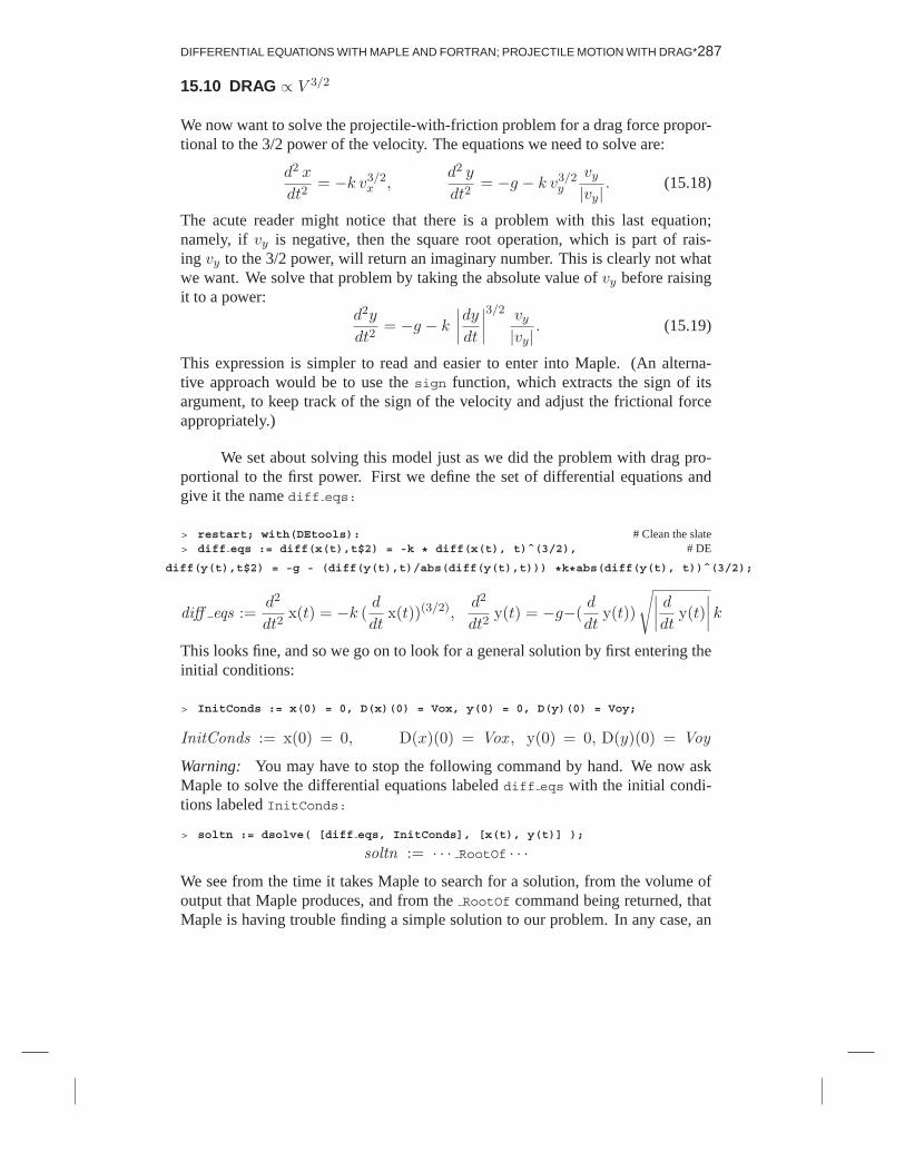
DIFFERENTIAL EQUATIONS WITH MAPLE AND FORTRAN; PROJECTILE MOTION WITH DRAG*287
15.10 DRAG ∝ V 3/2
We now want to solve the projectile-with-friction problem for a drag force propor-tional to the 3/2 power of the velocity. The equations we need to solve are:
d2 x
dt2= −k v3/2
x ,d2 y
dt2= −g − k v3/2
y
vy|vy|
. (15.18)
The acute reader might notice that there is a problem with this last equation;namely, if vy is negative, then the square root operation, which is part of rais-ing vy to the 3/2 power, will return an imaginary number. This is clearly not whatwe want. We solve that problem by taking the absolute value of vy before raisingit to a power:
d2y
dt2= −g − k
∣∣∣∣dydt∣∣∣∣3/2 vy
|vy|. (15.19)
This expression is simpler to read and easier to enter into Maple. (An alterna-tive approach would be to use the sign function, which extracts the sign of itsargument, to keep track of the sign of the velocity and adjust the frictional forceappropriately.)
We set about solving this model just as we did the problem with drag pro-portional to the first power. First we define the set of differential equations andgive it the name diff eqs:
> restart; with(DEtools): # Clean the slate> diff eqs := diff(x(t),t$2) = -k * diff(x(t), t)ˆ(3/2), # DE
diff(y(t),t$2) = -g - (diff(y(t),t)/abs(diff(y(t),t))) *k*abs(diff(y(t), t))ˆ(3/2);
diff eqs :=d2
dt2x(t) = −k (
d
dtx(t))(3/2),
d2
dt2y(t) = −g−(
d
dty(t))
√∣∣∣∣ ddt y(t)∣∣∣∣ k
This looks fine, and so we go on to look for a general solution by first entering theinitial conditions:
> InitConds := x(0) = 0, D(x)(0) = Vox, y(0) = 0, D(y)(0) = Voy;
InitConds := x(0) = 0, D(x)(0) = Vox , y(0) = 0, D(y)(0) = Voy
Warning: You may have to stop the following command by hand. We now askMaple to solve the differential equations labeled diff eqs with the initial condi-tions labeled InitConds:
> soltn := dsolve( [diff eqs, InitConds], [x(t), y(t)] );
soltn := · · · RootOf · · ·We see from the time it takes Maple to search for a solution, from the volume ofoutput that Maple produces, and from the RootOf command being returned, thatMaple is having trouble finding a simple solution to our problem. In any case, an
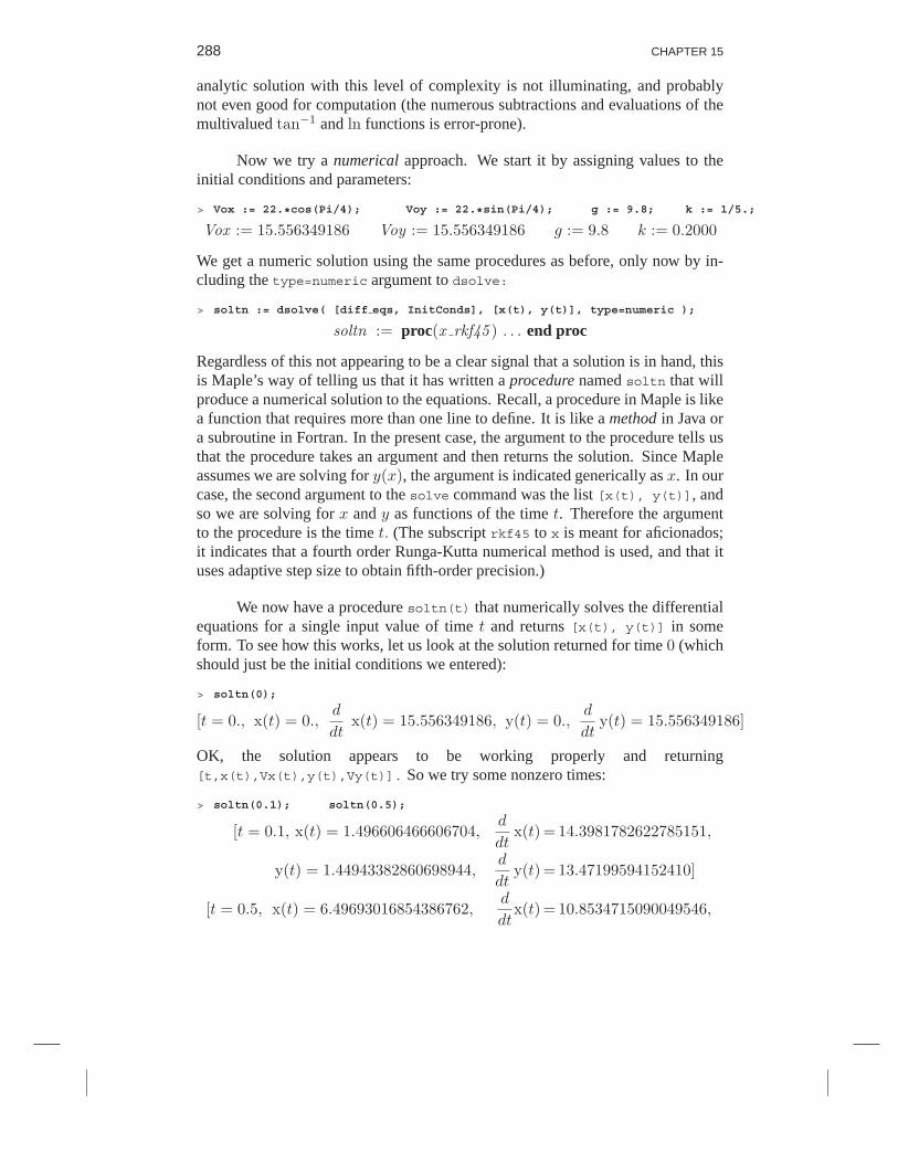
288 CHAPTER 15
analytic solution with this level of complexity is not illuminating, and probablynot even good for computation (the numerous subtractions and evaluations of themultivalued tan−1 and ln functions is error-prone).
Now we try a numerical approach. We start it by assigning values to theinitial conditions and parameters:
> Vox := 22.*cos(Pi/4); Voy := 22.*sin(Pi/4); g := 9.8; k := 1/5.;
Vox := 15.556349186 Voy := 15.556349186 g := 9.8 k := 0.2000
We get a numeric solution using the same procedures as before, only now by in-cluding the type=numeric argument to dsolve:
> soltn := dsolve( [diff eqs, InitConds], [x(t), y(t)], type=numeric );
soltn := proc(x rkf45 ) . . . end proc
Regardless of this not appearing to be a clear signal that a solution is in hand, thisis Maple’s way of telling us that it has written a procedure named soltn that willproduce a numerical solution to the equations. Recall, a procedure in Maple is likea function that requires more than one line to define. It is like a method in Java ora subroutine in Fortran. In the present case, the argument to the procedure tells usthat the procedure takes an argument and then returns the solution. Since Mapleassumes we are solving for y(x), the argument is indicated generically as x. In ourcase, the second argument to the solve command was the list [x(t), y(t)], andso we are solving for x and y as functions of the time t. Therefore the argumentto the procedure is the time t. (The subscript rkf45 to x is meant for aficionados;it indicates that a fourth order Runga-Kutta numerical method is used, and that ituses adaptive step size to obtain fifth-order precision.)
We now have a procedure soltn(t) that numerically solves the differentialequations for a single input value of time t and returns [x(t), y(t)] in someform. To see how this works, let us look at the solution returned for time 0 (whichshould just be the initial conditions we entered):
> soltn(0);
[t = 0., x(t) = 0.,d
dtx(t) = 15.556349186, y(t) = 0.,
d
dty(t) = 15.556349186]
OK, the solution appears to be working properly and returning[t,x(t),Vx(t),y(t),Vy(t)]. So we try some nonzero times:
> soltn(0.1); soltn(0.5);
[t = 0.1, x(t) = 1.496606466606704,d
dtx(t) = 14.3981782622785151,
y(t) = 1.44943382860698944,d
dty(t) = 13.47199594152410]
[t = 0.5, x(t) = 6.49693016854386762,d
dtx(t) = 10.8534715090049546,
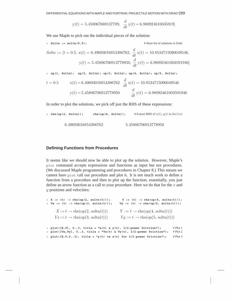
DIFFERENTIAL EQUATIONS WITH MAPLE AND FORTRAN; PROJECTILE MOTION WITH DRAG*289
y(t) = 5.458067069137789,d
dty(t) = 6.980924610035919]
We use Maple to pick out the individual pieces of the solution:
> Soltn := soltn(0.5); # Store list of solutions in Soltn
Soltn := [t = 0.5, x(t) = 6.49693016854386762,d
dtx(t) = 10.8534715090049546,
y(t) = 5.45806706913778950,d
dty(t) = 6.98092461003591946]
> op(1, Soltn); op(2, Soltn); op(3, Soltn); op(4, Soltn); op(5, Soltn);
t = 0.5 x(t) = 6.49693016854386762d
dtx(t) = 10.8534715090049546
y(t) = 5.45806706913778950d
dty(t) = 6.98092461003591946
In order to plot the solutions, we pick off just the RHS of these expressions:
> rhs(op(2, Soltn)); rhs(op(4, Soltn)); # Extract RHS of x(t), y(t) in Soltn
6.49693016854386762 5.45806706913778950
Defining Functions from Procedures
It seems like we should now be able to plot up the solution. However, Maple’splot command accepts expressions and functions as input but not procedures.(We discussed Maple programming and procedures in Chapter 8.) This means wecannot have plot call our procedure and plot it. It is not much work to define afunction from a procedure and then to plot up the function; essentially, you justdefine an arrow function as a call to your procedure. Here we do that for the x andy positions and velocities:
> X := (t) -> rhs(op(2, soltn(t))); Y := (t) -> rhs(op(4, soltn(t)));> Vx := (t) -> rhs(op(3, soltn(t))); Vy := (t) -> rhs(op(5, soltn(t)));
X := t → rhs(op(2, soltn(t))) Y := t→ rhs(op(4, soltn(t)))Vx := t → rhs(op(3, soltn(t))) Vy := t → rhs(op(5, soltn(t)))
> plot([X,Y], 0..3, title = "x(t) & y(t), 3/2-power friction"); # Plot 1> plot([Vx,Vy], 0..3, title = "Vx(t) & Vy(t), 3/2-power friction"); # Plot 2
> plot([X,Y,0..3], title = "y(t) vs x(t) for 3/2-power friction"); # Plot 3

290 CHAPTER 15
Figure 15.1 Left: The gravitational force on a planet a distance r from the sun. The x and ycomponents of the force are indicated. Right: Output from the applet PlanetRHLshowing the precession of a planet’s orbit when the gravitational force ∝ 1/r4.
x(t) & y(t), 3/2-power friction
–5
0
5
10
15
20
0.5 1 1.5 2 2.5 3
Vx(t) & Vy(t), 3/2-power friction
–10
–5
0
5
10
15
0.5 1 1.5 2 2.5 3
y(t) vs x(t) for 3/2-power friction
–4
–2
0
2
4
6
5 10 15 20
We see similar results to Model 1, only now with an even more drastic “drop outof the sky effect” at the end of the trajectory.
15.11 EXPLORATION: PLANETARY MOTION*
Newton’s explanation of the motion of the planets in terms of a universal law ofgravitation is one of the great achievements of science. He was able to provethat the planets traveled along elliptical paths with the sun at one vertex, and withperiods that agree with observation. All Newton needed to postulate is that theforce between a planet of mass m and the sun of mass M is given by
F = −GmM
r2, (15.20)
where r is the distance between the planet of mass m and sun of mass M , and Gis a universal constant. The minus sign indicates that the force is always attrac-tive and lies along the line connecting the planet and sun, as indicated on the leftof Figure 15.1. The hard part for Newton was solving the resulting differentialequations, since he had to invent calculus to do it. Whereas the analytic solution iscomplicated, the numerical solution is not.

DIFFERENTIAL EQUATIONS WITH MAPLE AND FORTRAN; PROJECTILE MOTION WITH DRAG*291
Even for planets, the basic equation of motion is
F = ma = md2xdt2
, (15.21)
with the force now given by (15.20). If we look at Figure 15.1 we see that
Fx = F cos θ = Fx
r, Fy = F sin θ = F
y
r, r =
√x2 + y2,
(15.22)with F given by (15.20). If we write the equation of motion in component form andsubstitute (15.22) for the force components, we obtain the differential equations weneed to solve:
d2x
dt2= −GM
x
r3,
d2y
dt2= −GM
y
r3. (15.23)
Implementation: Planet.java*
On the Java section of the CD you will find the applet Planet. Although this isJava based, you can run the applet with just a browser. We suggest that you run theclass file to see how the solution behaves. To keep the calculation simple withoutchanging the physics, assume that the units we use are such that GM = 1, andthat the initial conditions are [Feyn 63]:
x(0) = 0.5, y(0) = 0, vx(0) = 0.0, vy(0) = 1.63. (15.24)
1. Modify projectileAir.java so that it solves (15.23) as functions of time.2. Make the number of time steps large enough so that the planet’s orbit repeats
on top of itself.3. You may need to make the time step small enough so that the orbit closes
upon itself (it should) and just repeats. This should be a nice ellipse.4. Experiment with initial conditions until you obtain the ones that produce a
circular orbit (a circle is a special case of an ellipse).5. Once you have good precision, see the effect of progressively increasing the
initial velocity until the orbit opens up and becomes an hyperbola.6. Use the same initial conditions as produced the ellipse. This time investigate
the effect of the power in (15.20) being 1/r4 rather than 1/r2. You shouldfind that the orbital ellipse now rotates (precesses), as in Figure 15.1.
15.12 KEY WORDS
equations of motion Euler’s method forward differencenumerical ODE solution numerical differentiation ODE

292 CHAPTER 15
15.13 SUPPLEMENTARY EXERCISES
1. Use Maple, Fortran, or both to find the solution of the differential equation
dn(t)dt
= −λn(t), (15.25)
with the initial condition n(0) = 100. Plot up the answer for λ = 0.3.2. In Chapter 16 you will encounter an RLC electrical circuit and the differ-
ential equation describing it. We consider here the same circuit without acapacitor and described by the differential equation
V (t) = RI + LdI
dt. (15.26)
Solve this equation for the current in the circuit for the same values of R andL as in the problem, and for a constant V (t) (same magnitude as in problem).Plot your solution.
3. Consider exponential growth starting with an initial population N(0) = 2.a. Solve the equation describing exponential growth
dN(t)dt
= λN(t). (15.27)
Assign the integration constants to correspond to n(0) = 100, and λ =0.3, and plot up the solution.
b. Solve for exponential growth with a modulated growth parameter
dy(t)dt
= λ
[10000−N(t)
10000
]×N(t). (15.28)
This is the differential-equation version of the logistics map studied inChapter 19, “Discrete Math, Arrays as Bins.” The term in square bracketsis insignificant for small N(t).
4. Solve for and plot up the solution to the differential equation
dy(x)dx
= sin(xy), (15.29)
with initial condition y(0) = 1.a. Verify that Maple cannot find an analytic solution to this equation.b. Have Maple find a numerical solution to this equation.
5. Solve for and plot up the solution to the differential equation
d2y(x)dx2
= −y(x)3, (15.30)
subject to the initial conditions y(0) = 1, y′(0) = 0. Hint: If Maple cannotfind an analytic solution, you may need to try a numerical one.

Chapter Sixteen
Object-Oriented Programming, Abstract Data;
Complex Currents*
Note to the instructor: As an alternative to the full version of this chapter, you mayskip the study of the RLC circuit and just focus on the mathematics of complexnumbers and their representation in terms of objects. And even with that, you maydefer the use of nonstatic (object-oriented) methods to a later time.
16.1 PROBLEM: RESONANCE IN RLC CIRCUIT
We are given the circuit shown on the left of Figure 16.1 containing a resistor ofresistance R, an inductor of inductance L, and a capacitor of capacitance C. Allthree elements are connected in series to an alternating voltage source
V (t) = V0 cosωt. (16.1)
Problem: Determine the magnitude and time dependence of the current in thisRLC circuit as a function of the frequency of the external voltage. We will solvethe RLC circuit problem for you within this chapter. Your problem is to repeat thecalculation for a circuit in which there are two RLC circuits in parallel, as shownon the right of Figure 16.1. You may assume a single value for inductance andcapacitance, and three values for resistance:
L = 1000 H, C =1
1000F, R =
10001.5
,10002.1
,10005.2
Ω. (16.2)
Consider frequencies of applied voltage in the range 0 < ω < 2/√LC = 2/s.
16.2 MATH: COMPLEX NUMBERS
Try to remember your first exposure to square roots in elementary school. Thoughit was straightforward to understand that 52 = 25, it was a challenge to understandthat
√25 = ±5, and more of a challenge to understand what was the true value of√
24. For many of us, it was downright impossible to understand the true value of√−1. Mathematicians, being a rather clever and proud bunch, have handled this

294 CHAPTER 16
!
!
!
Figure 16.1 Left: An RLC circuit connected to an alternating voltage source. Right: Two RLCcircuits connected in parallel to an alternating voltage. Observe that one of the parallelcircuits has double the values of R, L, and C as does the other.
affront to their abilities by inventing the number i as the answer,1
idef=
√−1, i2 = −1, (16.3)
where the “def” over the equal sign indicates a definition. In this way mathemati-cians have a way of going ahead with their calculations, even if they do not knowwhat i means. Whereas defining away one’s ignorance may appear to be a swindle,mathematicians are an honest bunch at heart and so tell the world that they havereally just made up the answer by calling i the imaginary number. “Imaginary” isa good name for i, since there is no way to measure this number in the real world,but, then again, there is no law forbidding us from imagining such a number.
In common mathematical usage, i is called the imaginary number, while anymultiple of i is called an imaginary number. So, for example, 2i, i, and 100i are allimaginary numbers. Once we have extended our minds to imagine an imaginarynumber, it is not much of a stretch to imagine adding a real number to an imaginarynumber to form something more complex. To name an instance, 1 + i, 1 + 2i, and100 + 76i. These numbers with both real and imaginary parts are called complexnumbers.2 The term “complex” indicates that these numbers have a number ofparts, and not that they are hard to understand!
Complex numbers are very useful in mathematics and science since they letus double our work output with only the slightest increase in input. This is accom-plished by employing the familiar operations of algebra and calculus on complexnumbers, and then separating off the real and imaginary parts of the answer atthe end. By way of example, even if z is a complex number, z3/z still equal z2,without our having to express the individual numbers in terms of their real andimaginary parts.
1The invention is credited to Girolama Cardana (1501–1576).2The term, as well as much in applied mathematics, is credited to Carl Friedrich Gauss (1777–1855).

OBJECT-ORIENTED PROGRAMMING, ABSTRACT DATA; COMPLEX CURRENTS* 295
θ
Figure 16.2 Representation of a complex number as a vector in space.
To do algebra with complex numbers, we define the symbol z to represent anumber with both real and imaginary parts:
z = x + iy. (16.4)
In turn, the complex nature of z is indicated by giving its real and imaginary parts:
Re z = x, Im z = y. (16.5)
In a strict sense, y is the magnitude of the imaginary part of z, and iy is the imagi-nary part. Yet y is usually called “the imaginary part.”
Because complex numbers have independent real and imaginary parts, a use-ful way to visualize them is to imagine a coordinate system in which the ordinatepoints off into imaginary space and the abscissa points off into real space. As seenin Figure 16.2, we then visualize z = x + iy as a point with y projection alongthe imaginary axis and x projection along the real axis. This is analogous to avector in a 2-D space, except that part of this vector lies in an imaginary space.The analogy between complex numbers and 2-D vectors is taken one step furtherby applying the polar coordinate representation of a vector to complex numbers.On account of this, the point z in Figure 16.2 may be located not only by givingits Cartesian coordinates x and y, but also by specifying it polar coordinates r,the length of the vector from the origin to point z, and θ, the angle that the vectormakes with the abscissa. The complex number is the same in either case, and,indeed, the two representations are related via simple trigonometry:
r =√x2 + y2, θ = tan−1(y/x),
x = r cos θ, y = r sin θ.(16.6)

296 CHAPTER 16
Complex Arithmetic Review
The essence of the computing aspect of our problem is the programming of therules of arithmetic for complex numbers. This is an interesting chore becausewhile Java contains all the rules for real numbers, you must educate Java as to therules for complex numbers. Indeed, since complex numbers are not primitive datatypes like doubles and floats, we will construct complex numbers as objects.3
We start with two complex numbers, which we distinguish with subscripts:
z1 =x1 + i y1, (16.7)
z2 =x2 + i y2. (16.8)
The rules of arithmetic follow by applying algebra to the real and imaginary parts:
Addition: z1 + z2 = (x1 + x2) + i(y1 + y2), (16.9)
Subtraction: z1 − z2 = (x1 − x2) + i(y1 − y2), (16.10)
Multiplication: z1 × z2 = (x1 + iy1)× (x2 + iy2), (16.11)
= (x1x2 − y1y2) + i(x1y2 + x2y1),
Division: z1z2
=x1 + iy1
x2 + iy2× x2 − iy2
x2 − iy2, (16.12)
=(x1x2 + y1y2) + i(y1x2 − x1y2)
x22 + y2
2
.
In deducing the rule for complex division we employed the fact that a complexnumber z multiplied by its complex conjugate
z∗ = x− iy, (16.13)
always yields a real number:
z × z∗ = (x + iy)(x− iy) = x2 + y2. (16.14)
We observe that this result is the same as the square of the length r defined in(16.6). The length r is commonly referred to as the modulus or magnitude of thecomplex number z, and is expressed by using the absolute value symbol: r = |z|.The product of the complex number z and its complex conjugate z∗ is then
zz∗ = |z|2 = r2. (16.15)
Exercise: Consider the complex numbers
b = 1 + 2i, c = 4 + i. (16.16)
What are the values of b + c, b− c, b× c, |c|, and b/c? ♠
3Because complex numbers are used so often in science and engineering, there is a move afoot to have somefuture versions of Java incorporate complex numbers as a primitive data type in order to speed up execution andmake them easier to use.
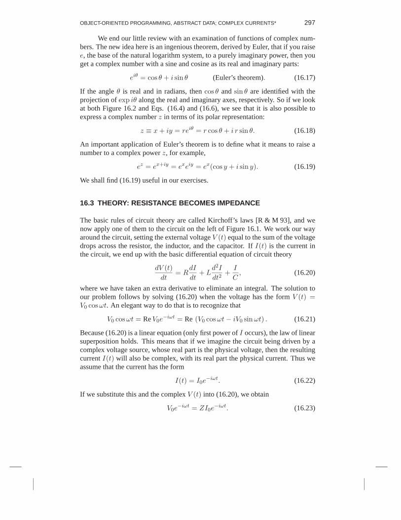
OBJECT-ORIENTED PROGRAMMING, ABSTRACT DATA; COMPLEX CURRENTS* 297
We end our little review with an examination of functions of complex num-bers. The new idea here is an ingenious theorem, derived by Euler, that if you raisee, the base of the natural logarithm system, to a purely imaginary power, then youget a complex number with a sine and cosine as its real and imaginary parts:
eiθ = cos θ + i sin θ (Euler’s theorem). (16.17)
If the angle θ is real and in radians, then cos θ and sin θ are identified with theprojection of exp iθ along the real and imaginary axes, respectively. So if we lookat both Figure 16.2 and Eqs. (16.4) and (16.6), we see that it is also possible toexpress a complex number z in terms of its polar representation:
z ≡ x + iy = reiθ = r cos θ + i r sin θ. (16.18)
An important application of Euler’s theorem is to define what it means to raise anumber to a complex power z, for example,
ez = ex+iy = exeiy = ex(cos y + i sin y). (16.19)
We shall find (16.19) useful in our exercises.
16.3 THEORY: RESISTANCE BECOMES IMPEDANCE
The basic rules of circuit theory are called Kirchoff’s laws [R & M 93], and wenow apply one of them to the circuit on the left of Figure 16.1. We work our wayaround the circuit, setting the external voltage V (t) equal to the sum of the voltagedrops across the resistor, the inductor, and the capacitor. If I(t) is the current inthe circuit, we end up with the basic differential equation of circuit theory
dV (t)dt
= RdI
dt+ L
d2I
dt2+
I
C, (16.20)
where we have taken an extra derivative to eliminate an integral. The solution toour problem follows by solving (16.20) when the voltage has the form V (t) =V0 cosωt. An elegant way to do that is to recognize that
V0 cosωt = ReV0e−iωt = Re (V0 cosωt− iV0 sinωt) . (16.21)
Because (16.20) is a linear equation (only first power of I occurs), the law of linearsuperposition holds. This means that if we imagine the circuit being driven by acomplex voltage source, whose real part is the physical voltage, then the resultingcurrent I(t) will also be complex, with its real part the physical current. Thus weassume that the current has the form
I(t) = I0e−iωt. (16.22)
If we substitute this and the complex V (t) into (16.20), we obtain
V0e−iωt = ZI0e
−iωt. (16.23)

298 CHAPTER 16
Here Z is called the impedance and is the complex expression
Z = R + i
(1ωC
− ωL
). (16.24)
Equation (16.23) is the generalization of Ohm’s law, V = IR, to alternating cur-rent circuits.4 We see that the real part of the impedance is just the resistance R,while the imaginary part (called the reactance) is 1/ωC − ωL. As we shall see,the imaginary part of the impedance determines the phase of the current.
Solution for Complex Current
If we now solve (16.23) for the complex current, we obtain
I(t) =1ZV0e
−iωt =V0e
−iωt
R + i (1/ωC − ωL). (16.25)
Eq. (16.25) is more illuminating if the complex impedance is expressed in polarform:
Z = |Z|eiθ, (16.26)
|Z| =√R2 + (1/ωC − ωL)2, θ = tan−1
(1/ωC − ωL
R
). (16.27)
We see now that the complex current is
I(t) =V0
|Z|e−i(ωt+θ), (16.28)
which means that the physical current is its real part:
Iphysical(t) = ReI(t) =V0
|Z| cos(ωt + θ). (16.29)
Equation (16.29) states that the amplitude of the current in the circuit is given bythe amplitude of the voltage divided by the magnitude of the complex impedance,and that the phase of the current, relative to that of the voltage, is given by θ. If thephase θ > 0, then the current leads the voltage in time, that is, the current reachesits maximum before the voltage reaches its maximum. If θ is negative, then thecurrent lags the voltage.
Finally, what is to be done if we have two such RLC circuits in parallel,as shown on the right of Figure 16.1. The analysis is the same as that done withordinary resistors. If two impedances are in series, then they have the same currentpassing through them. If two impedances are in parallel, then they have the same
4Some elementary texts may refer to |Z| as the impedance and then use the concept of phasors to describe theeffect of the impedance on the phase. We view the use of complex impedance as more direct and elegant.

OBJECT-ORIENTED PROGRAMMING, ABSTRACT DATA; COMPLEX CURRENTS* 299
Figure 16.3 An abstract drawing, or what?
voltage across them. If two impedances are connected in series, then the voltagesadd, and this leads to:
Z = Z1 + Z2 (series connection). (16.30)
If the impedances are connected in parallel, then the currents add, and this leads to
1Z
=1Z1
+1Z2
(parallel connection). (16.31)
Hence in the parallel case, the impedances add in inverse, with all the steps of thecalculation being performed with complex arithmetic.
16.4 CS: ABSTRACT DATA TYPES, OBJECTS
What do you see when you look at the abstract object in Figure 16.3? Somereaders may see a face in profile, others may see some parts of human anatomy,and others the total absence of artistic ability. This figure is abstract in the sensethat it does not try to present a true or realistic picture of the object, but rather usesa symbol to suggest more than meets the eye.
Abstract or formal concepts pervade mathematics and science because theymake it easier to describe nature. For example, we often use the symbol v(t) todenote the velocity of an object as a function of time. Despite velocity being afamiliar concept, it is actually abstract in the sense that we cannot see it. What wesee is the position of the object as a function of time, and then we infer from thatthe velocity by determining how rapidly that position is changing.
In computer science (CS), we create an abstract object by using a symbol todescribe a collection of items. We have already seen that data, or variables in Javaor Fortran may be integers, floating-point numbers, Booleans, or strings. Thesetypes of variables are built into the languages and therefore are called primitivedata types. In addition, computer languages let the user define abstract data typesof their own by combining primitive data types into more complicated structurescalled objects. These objects are abstract in the sense that they are named with asingle symbol, yet they represent a number of parts.

300 CHAPTER 16
For instance, one might create an object with parts that contain a student’sschool record (ID, grades, etc.), as well as other parts that contain methods to cal-culate the grade point average, etc. Of course, one would need many such objectsbecause there are many students. To distinguish between the general structure ofthis student-record object and specific record objects for individual students, thegeneral object is called a class, while the object for specific cases is called aninstance of the class, or just an object.
In this chapter, our objects will be complex numbers, while in other chaptersthey may be plots, vectors, or matrices. The classes that we form will be combina-tions of abstract data types and associated methods for modifying those data. Theentire class may also be thought of as objects. In a formal sense, computer sciencerequires abstract data types to possess the three properties [Zach 96]:
Typename: procedure to construct the new data type from elementary pieces.
Set values: mechanism for assigning values to the defined data type.
Set operations: rules that permit operations on the new data type (you would nothave gone to all the trouble of declaring a new data type unless you were interestedin doing something with it).
In terms of these properties, when we declare a variable to be complex we satisfyproperty (1). When we declare Rez = x and Imz = y as doubles, we satisfy (2).When we define the rules of arithmetic and trigonometry for complex numbers (asreviewed in § 16.2), we satisfy (3).
Before we examine how these properties are applied in our programs, let usreview the structure we have been using in our Java programs. When we start offour programs with a declaration statement such as double x. This tells the Javacompiler the kind of variable x is, so that Java will store it properly in memoryand use proper operations on it. The general rule is that every variable we use ina program must have its data type declared. For primitive (built-in) data types, wedeclare them to be double, float, int, char, long, short, or boolean.
If our program employs some user-defined, abstract data types, then theytoo must be declared. This declaration must occur even if we do not define themeaning of the data type until later in the program (the compiler checks on that).Consequently, when our program refers to a number z as complex, the compilermust be told at some point that there is both a real part x and an imaginary part ythat makes up a complex number.

OBJECT-ORIENTED PROGRAMMING, ABSTRACT DATA; COMPLEX CURRENTS* 301
16.5 OBJECTS IN FORTRAN
One of the powerful and modern aspects of Fortran is its object-oriented approachto programming. Since the new concepts of object-oriented programming (OOP)can be a rather hard to grasp as purely theoretical concepts, we will gain someexperience with objects and in the process learn some of the concepts of OOP.After all, a child learns to speak a language in a similar way!
For present purposes, it is easiest to think of an object in Fortran as a non-primitive data type with a number of specified components. Examples will includecomplex numbers and arrays. Indeed, when we set up a class file in Fortran con-taining our definition of a new, multi-component data type, and include variousmethods we have written to assign values to and operate on the new data type, wehave created an object. Actually the class file containing a collection of data (vari-able) definitions and the associated methods to operate on the data that we havebeen calling a class, is a version of an object.
Data by Reference
Before we start working with objects in a program, it is necessary to understandthat even though we may assign a variable name like x to an object, because ob-jects have multiple components, you do not assign one explicit value to the object.Indeed, since you are the one who defines just how big and complicated your ob-jects will be, it will also be your job to assign values to all of the different parts ofthe objects you create.
When Fortran deals with objects it does so by what computer scientists callby reference. More simply, when you refer toan object, Fortran understands that tomean that you are referring to the location in memory where your object is storedand not to the explicit values of the object’s parts. If you remember that objectsare referenced by their locations in memory rather than their actual values, theprocedures we are about to describe will make more sense.
Sample Data Type
We suspect that all the words in the preceding section mean little without a realexample to follow. So let’s now examine an example of an object in Fortran, afterwhich you should be able to go back and make more sense of the preceding words.The “object” that we will create with Fortran will be a complex number (aboutwhich, after sections § 16.2-16.2, you should be an expert). Despite the fact thatFortran has its own intrinsic complex data type, we create a custom data type for

302 CHAPTER 16
its instructive attributes.
Below we present the Fortran class file ComplexType.f90 that producescomplex-number objects:
Listing 16.1 ComplexType.f90
1 ! ComplexType . f90 : Using complex p r o c e d u r e s and t y p e d e f i n i t i o n s2 ! −−−−−−−−−−−−−−−−−−−−−−−−−−−−−−−−−−−−−−−−−−−−−−−−−−−−−−3 Module complex module4 ! D e f i n e complex t y p e5 Type p u b l i c c o m p l e x6 Rea l : : re , im7 End Type p u b l i c c o m p l e x8 ! Add t h e f u n c t i o n s f o r complex m a t h e m a t i c s9 C o n t a i n s
10 ! −−−−−− Add two complex numbers11 F u n c t i o n add ( a , b )12 I m p l i c i t None13 Type ( p u b l i c c o m p l e x ) , i n t e n t ( i n ) : : a , b14 Type ( p u b l i c c o m p l e x ) : : add15 add%r e = a%r e + b%r e16 add%im = a%im + b%im17 End F u n c t i o n add18 ! −−−−−− S u b t r a c t b from a complex numbers19 F u n c t i o n s u b t r a c t ( a , b )20 I m p l i c i t None21 Type ( p u b l i c c o m p l e x ) , i n t e n t ( i n ) : : a , b22 Type ( p u b l i c c o m p l e x ) : : s u b t r a c t23 s u b t r a c t%r e = a%r e − b%r e24 s u b t r a c t%im = a%im − b%im25 End F u n c t i o n s u b t r a c t26 ! −−−−−− M u l t i p l y two complex numbers27 F u n c t i o n m u l t i p l y ( a , b )28 I m p l i c i t None29 Type ( p u b l i c c o m p l e x ) , i n t e n t ( i n ) : : a , b30 Type ( p u b l i c c o m p l e x ) : : m u l t i p l y31 m u l t i p l y%r e = a%r e ∗ b%r e − a%im ∗ b%im32 m u l t i p l y%im = a%r e ∗ b%im + a%im ∗ b%r e33 End F u n c t i o n m u l t i p l y34 ! −−−−−− D i v i d e two complex numbers35 F u n c t i o n d i v i d e ( a , b )36 I m p l i c i t none37 Type ( p u b l i c c o m p l e x ) , i n t e n t ( i n ) : : a , b38 Type ( p u b l i c c o m p l e x ) : : d i v i d e39 d i v i d e%r e = ( a%r e ∗ b%r e + a%im ∗ b%im ) / ( b%r e ∗∗2 + b%im ∗∗2)40 d i v i d e%im = ( a%im ∗ b%r e − a%r e ∗ b%im ) / ( b%r e ∗∗2 + b%im ∗∗2)41 End F u n c t i o n d i v i d e42 End Module complex module43 !44 Program Main program45 Use complex module46 I m p l i c i t None

OBJECT-ORIENTED PROGRAMMING, ABSTRACT DATA; COMPLEX CURRENTS* 303
47 Type ( p u b l i c c o m p l e x ) : : a , b , c48 C h a r a c t e r ch49 a%r e =1 .50 a%im =2 .51 b%r e =3 .52 b%im =4 .53 i f ( a%im >=0.0) t h e n54 ch = ’+’55 e l s e i f ( a%im <0.0) t h e n56 ch = ’-’57 end i f58 w r i t e (∗ ,∗ ) ’a = ’ , a%re , ch , abs ( a%im ) , ’i’59 i f ( b%im >=0.0) t h e n60 ch = ’+’61 e l s e i f ( b%im <0.0) t h e n62 ch = ’-’63 end i f64 w r i t e (∗ ,∗ ) ’b = ’ , b%re , ch , abs ( b%im ) , ’i’65 c = add ( a , b )66 i f ( c%im >=0.0) t h e n67 ch = ’+’68 e l s e i f ( c%im <0.0) t h e n69 ch = ’-’70 end i f71 w r i t e (∗ ,∗ ) ’a + b = ’ , c%re , ch , abs ( c%im ) ,’i’72 c = s u b t r a c t ( a , b )73 i f ( c%im >=0.0) t h e n74 ch = ’+’75 e l s e i f ( c%im <0.0) t h e n76 ch = ’-’77 end i f78 w r i t e (∗ ,∗ ) ’a - b = ’ , c%re , ch , abs ( c%im ) ,’i’79 c = m u l t i p l y ( a , b )80 i f ( c%im >=0.0) t h e n81 ch = ’+’82 e l s e i f ( c%im <0.0) t h e n83 ch = ’-’84 end i f85 w r i t e (∗ ,∗ ) ’a * b = ’ , c%re , ch , abs ( c%im ) ,’i’86 i f ( b%r e ==0. .AND. b%im = = 0 . ) t h e n87 w r i t e (∗ ,∗ ) ’Error: division by zero ’ , b%re ,’+’ , b%im ,’i’88 e l s e89 c = d i v i d e ( a , b )90 i f ( c%im >=0.0) t h e n91 ch = ’+’92 e l s e i f ( c%im <0.0) t h e n93 ch = ’-’94 end i f95 w r i t e (∗ ,∗ ) ’a / b = ’ , c%re , ch , abs ( c%im ) ,’i’96 end i f97 End Program main program

304 CHAPTER 16
Exercise:
1. The program ComplexType.f90 provides all Abelian algebraic operations oncomplex numbers, with the complex numbers represented as objects. Enterthe ComplexType.f90 program file by hand, trying to understand it as bestyou can in the process.
2. Compile and execute this program, and check that the output agrees with theresults you obtained in the exercises in §16.2.
The first thing to notice about ComplexType.f90 is that the data type isdeclared with the statements
5. Type public complex
6. Real :: re, im
7. End Type public complex
The main program is declared on line 44 with
44. Program Main program
These are the same techniques we have employed before (it’s good when somethings stay the same in life). However, on line 6 we see that the variables re andim are declared for the public data type with the statement
6. Real :: re, im
These variables are part of a dynamicdata type, an object. These variables aredynamic in thesense that they will be different for each object (instance of theclass) created. That is, if we define z1 and z2 to be Complex objects, then thevariables re and im will be different for z1 and z2.
We extract the component parts of our complex object by a projection op-eration. [For those readers who know some vector analysis, you can think of thisas similar to extracting the components of a vector in space by taking dot prod-ucts with the unit vectors to project the vector onto different axes.] The projectionoperation is denoted by a %:

OBJECT-ORIENTED PROGRAMMING, ABSTRACT DATA; COMPLEX CURRENTS* 305
z1%re real part of object z1z1%im imaginary part of object z1z2%re real part of object z2z2%im imaginary part of object z1
Object Constructors
To construct an object from a module in Fortran, one must simply state the use ofthe module before any other declarations, such as in ComplexType.f90.
45. Use complex module
Some explanation is clearly in order! Modules are covered in more details in Chap-ter 18. Briefly now, a module acts like a nested class in Fortran. A module can beused by other programs once it has been compiled. All of the procedures in a mod-ule are static. A procedure or variable can be declared private, protected, or public.The declaration of user rights to the module’s constituents is important only if youare developing programs with security in mind. Once a module is used inside ofa procedure or program, all of the module’s procedures and data types becomeavailable for use therein. For example, look at the program ComplexType.f90 fora demonstration of multiple functions that may be used by other programs via themodule complex module.
Exercise Add two functions to complex module that allow a user to create a de-fault complex number and a custom complex number from two real initial values.
Declaring and Creating Objects
Now let’s take stock of what we have up until this point. On line 6, our programhas defined the variables re and im that each object of this program will have. Forthis reason these variables that project the component parts are often referred toas instance variables. We also have a complex number algebra module that canperform algebraic operations on two complex numbers simultaneously.
In the main program, we can see how to create objects using the data typepublic complex. On line 47, in the usual place for declaring variables, we havethe statement
47. Type(public complex) :: a, b, c

306 CHAPTER 16
The compiler knows from the type command that public complex is notone of its primitive (built-in) data types. In the present case this program containsthe module named complex module with the data type public complex. Hence,the compiler does not have to look very far to know what you mean by a pub-lic complex data type5. Accordingly, when the statement Type(public complex)
:: a,b,c declares the variables a, b, and c to be public complex data objects,we know that they are manifestly objects since instanced data types are not static.
Recall that declaring a variable type, such as real or integer, does notassign a value to the variable, but, instead, tells the compiler to add the name ofthe variable to the list of variables it can be expected to encounter. Likewise, thedeclaration statement type(public complex) :: a,b,c lets the compiler knowwhat custom data type these variables are.
To actually create the objects, and not just register their names, we have toplace numerical values in the memory locations that have been reserved for theobjects. Since an object has multiple parts, we cannot give all its parts initialvalues with a simple assignment statement like a = 0;, so some other method isneeded.A new instance of a complex data type is created as above, then valuesare assigned by accessing the internal instance variables of the complex data typevariable.
49. a%re = 1. Sets the internal real part by reference
50. a%im = 2. Sets the internal imaginary part by reference
Instances
Since the name of the parent object and the names of objects that are created arethe same, it sometimes is useful to use yet another word to distinguish one fromthe other. Accordingly, the phrase instance of a class is used to refer to the cre-ated objects (in our example, a, b, and c), that is, the created objects are each asingle reference to the parent object. This designation distinguishes them from thedefinition of the abstract data type.
16.6 FORTRAN SOLUTION: COMPLEX CURRENTS
1. Extend the program ComplexType.f90 by adding new functions to subtract,take the modulus, take the complex conjugate, and determine the phase of
5Other Fortran files could also use our complex methods, but we have enough to worry about right now.
OBJECT-ORIENTED PROGRAMMING, ABSTRACT DATA; COMPLEX CURRENTS* 307
complex numbers.2. Test your methods by checking that the following identities hold for a variety
of complex numbers:
z + z = 2z, z + z∗ = 2 Rezz − z = 0, z − z∗ = 2 Imzzz∗ = |z|2, zz∗ = r2 (which is real)
(16.32)
Hint: Compare your output to some cases of pure real, pure imaginary, andsimple complex numbers that you are able to evaluate by hand.
3. Equations (16.29) and (16.27) are the solution for the current in a single RLCcircuit. It tells us that the magnitude of the current is given by
|I| =∣∣∣∣V0
Z
∣∣∣∣ , (16.33)
and that the phase of the current (relative to the cosωt time dependence) is
θI = tan−1(
1/ωC − ωL
R
). (16.34)
Modify the given complex arithmetic program so that it performs the com-plex arithmetic required by (16.33). Hint: You do not have to solve thisfrom scratch! Instead, use the techniques you have already programmed fordetermining the magnitude to determine |I|.
4. Compute and then make a plot of the magnitude and the phase of the currentin the circuit as a function of frequency ω of the external voltage source. Forour problem, a good range is 0 ≤ ω ≤ 2.
5. Assessment: You should notice a resonance peak in the magnitude at thesame frequency for which the phase vanishes. The smaller the resistance R,the sharper should the circuit pass through resonance. These types of circuitswere used in the early days of radio to tune to a specific frequency. Thesharper the peak, the better the quality of reception.
6. The second part of the problem dealing with the two circuits in parallel isvery similar to the first part. You need to change only the value of the im-pedance Z used. To do that, explicitly perform the complex arithmetic im-plied by (16.31), deduce a new value for the impedance, and then repeat thecalculation of the current.
16.7 MAPLE SOLUTION: COMPLEX CURRENTS
Recall from way back in Chapter 3 that Maple knows all about complex numbersand complex arithmetic. Indeed, you have probably already seen an occasional Ipop up as the solution to some equations. The point here is that Maple reserves thesymbol I as the
√−1, and this lets us use its I at our pleasure:
> restart: ‘sqrt (-1)‘ = sqrt (-1); # What’s returned?
308 CHAPTER 16
sqrt ( −1 ) = I
> expand((a + I*b)ˆ2); # See if Maple uses I as√−1
a2 + 2 I a b− b2
In §16.3 we applied circuit theory and complex analysis to the RLC circuit andfound that if the exciting voltage is the real part of
V (t) = V0 e(−I ω t), (16.35)
then the current in the circuit is
I(t) =V0 cos(ω t− θ)
|Z| . (16.36)
Here Z is the complex impedance,
> Z := R + I * (1/(omega*C) - omega*L);
Z := R + (1
ω C− ω L) I.
We will start our Maple investigation by trying to determine magnitude |Z| andphase θ of Z using Maple’s capabilities for complex analysis. Whereas needing toknow the magnitude and phase of Z is just another way of saying that we need toknow Z in polar notation, we have Maple calculate these for us:
> Re(Z); Im(Z); # ReZ, ImZ
Re(R + (1
ω C− ω L) I) Im(R + (
1ω C
− ω L) I)
This is just a fancy way of giving us back the input. The problem is that Maple doesnot know that ω, R, L, and C are real, and so it cannot do the complex arithmetic.To tell Maple that the constants are real, we tell it what to assume:
> assume (R, real); assume(L, real); assume(C, real); assume (omega, real);> Re(Z); Im(Z); # Now check again
R˜1
ω˜C˜− ω˜L˜
It has taken some work, but now we are ready for some complex arithmetic. Lookat the polar form:
> polar(Z);
polar(√
R˜2 + (1
ω˜C˜− ω˜L˜)2, argument(R˜ + (
1ω˜C˜
− ω˜L˜) I))
This is giving us the correct magnitude, but Maple appears unable to compute thephase. This seems to be a Maple failure. However, we get it to work by combiningthe map and evalc commands:
OBJECT-ORIENTED PROGRAMMING, ABSTRACT DATA; COMPLEX CURRENTS* 309
> Polar := map( evalc, polar(Z) ); # Polar is variable name
Polar := polar(√
R˜2 + (1
ω˜C˜− ω˜L˜)2, arctan(
1ω˜C˜
− ω˜L˜, R˜))
Here map applies the procedure evalc to each element of polar(Z) and returns thepolar form (|Z|, θ). This simplifies the elements into the form needed. [It shouldnot be this hard!] We get separate expressions out for the real and imaginary partsby using the command op(numb,expression) to extract the numb-th operand fromexpression:
> op(1,Polar); op(2,Polar); # Extract operands√R˜2 + (
1ω˜C˜
− ω˜L˜)2 arctan(1
ω˜C˜− ω˜L˜, R˜)
The expressions we have just derived are the standard ones for the magnitude andthe phase of the impedance Z. However, since the current is proportional to 1/|Z|,we will plot 1/|Z|. We could compute 1/Z and work with that as well.
Maple’s Surface Plots of Complex Impedance
We want to examine the current that occurs in the RLC circuit as a function ofthe driving frequency. We have already discussed in Chapter 4 some of Maple’scommands for plotting complex functions. Irrespective of them being illuminating,for the problem given here, we first use plot3d to make the familiar z(x, y) surfaceplot of the magnitude and phase of the current as functions of both the frequencyof the external voltage ω and of the resistance R:
> restart: Zinv := 1/(R + I * (1/(omega*C) - omega*L)); # Compute 1/Z> L := 1000; C :=1/1000; # Assign numerical values
Zinv :=1
R + ( 1ω C − ω L) I
L := 1000 C :=1
1000
> assume (R, real); assume (omega, real); # Tell Maple the constants are real> Polar := map( evalc, polar(Zinv) ); # Convert 1/Z to polar form
> polar(1/((Rˆ2+(1000/omega-1000*omega)ˆ2)ˆ(1/2)),
> arctan(-1000/omega + 1000*omega, R));
Polar := polar
⎛⎝ 1√
R˜2 + (1000ω˜ − 1000ω˜)2
, arctan(−1000ω˜
+ 1000ω˜, R˜)
⎞⎠
> mag := op(1, Polar); op(2, Polar); # Extract magnitude, phase
mag :=1√
R˜2 + (1000ω˜ − 1000ω˜)2
arctan(−1000ω˜
+ 1000ω˜, R˜)

310 CHAPTER 16
Check out how the magnitude has a maximum when the external frequencyω = 1/
√LC . This is the resonance frequency. For our choice of constants this
corresponds to ω = 1. We now make some plots to see if this is true.
> op(1, Polar); with(plots):> plot3d(op(1, Polar), omega = 0..2, R = 200..1000, axes = BOXED); # 1/Z vs ω
00.5
11.5
2
omega~
200400
600800
1000
R~
00.0010.0020.0030.0040.005
> plot3d(op(2,Polar), omega=0..2, R=200..1000, axes = NORMAL); # θ vs ω
–1
0.51
200400
600800
1000
R~0.5
2
omega~
00.5
11.5
2
x
–1–0.5
00.5
1
y
0
0.004
0.008
0.012
0.016
Sure enough, the plot of 1/|Z| shows that the magnitude of the current has a max-imum at ω = 1. (It helps to grab and rotate these plots to see them better.) We alsosee that as the resistance R in the circuit is made smaller, the maximum currentbecomes progressively larger. The second plot of the phase shows that below reso-nance, ω < 1, the current lags the voltage, while above resonance the current leadsthe voltage. Another way to visualize complex functions is with the commandcomplexplot3d. It makes a 3-D visualization of a complex function of a com-plex argument. Here we do it by treating the frequency ω = x + iy as a complexnumber:
> with(plots): R := 1000;> complexplot3d( 1/(R+I*(1/(w*C)-w*L) ), w = 0-I..2+I, axes = BOXED); # 1/Z
We see in the right plot above that there is a sharp peak at x = Re(ω) = 1,

OBJECT-ORIENTED PROGRAMMING, ABSTRACT DATA; COMPLEX CURRENTS* 311
as expected. The color change indicates where Im(1/Z) changes sign. If welook closely at this graph we will also see that there is a maximum for a negativeimaginary value of ω. This is related to how long the resonance stays excited, astatement we do not try to prove here.
16.8 KEY WORDS
abstract data types reactance frequency imaginary numbercomplex conjugate constructor current default constructorcomplex arithmetic class impedance instance of objectinstance variable magnitude modulus nonstatic methodsnonstatic variable object voltage polar representationcomplex number reference call resonance user-defined data typesobject creation
16.9 FORTRAN AND MAPLE EXERCISES
1. Since Fortran actually has a primitive data type complex*4 or complex*8,rewrite ComplexType.f90 in Lst. 16.1 as a more simplified Fortran programusing the correct primitive data types. (In other words, complex objects donot have to be built). Call your modified code Complex.f90; compare resultswith ComplexType.f90.
2. Complex mathematics is much easier if we have the pure imaginary numberi =
√−1. Define a new complex variable i with a value equal to i. (In
Maple, this is just the built-in variable I .)3. Now that you have a specific variable for i, write some new methods that
compute the following functions of complex numbers (objects):a. exp(z) = ex+iy = exeiy = ex(cos y + i sin y)b. sin(z) = (eiz − e−iz)/2i
4. Verify that your methods work by trying some simple cases. (In Maple,compare to the built-in functions that also handle complex numbers.) Ex-amples of simple cases might be the use of complex numbers like z1, z2 =0, 1, i, 2, 2i, . . ., where you can easily figure out the answers.
5. Let z = 3 + 3√
(3)i.a. Determine |z| and check that you get 6.b. Determine the phase θ of z and check that you get θ = π/3.
6. Find Re(2−3i)2/(2+3i), Im(1/z2), |(1+z)/(1−z)|, and (2−3i)/(2+3i).7. Consider the complex number z = x + iy. Use gnuplot to make a surface
plot of Im cos(z) and Re cos(z).8. Consider the complex function f(z) = z3/(1 + z4).
a. Make a plot of f(x) versus x, that is, assume z is real and vary it alongthe real axis.
b. Make surface plots of Rez and Imz. Restrict the range of x and y valuesto lie close to where the “action” is.

Chapter Seventeen
Arrays I: Vectors, Matrices; Rigid-Body Rotations
Vectors and matrices play key roles in scientific computing. Indeed, much of so-called high-performance computing involves computations with very large arrays.These arrays may contain experimental data needing processing, or they may con-tain the results of a simulation in which the discrete nature of breaking space upinto small units leads naturally to the use of arrays. And since real-world prob-lems are often complicated and require high precision (small units), arrays withthousands or millions of elements are not unusual. Even though this means thatthe matrices used in realistic problems will be big and will require efficient algo-rithms, often the programs using matrices are simple and direct.
In this chapter, we deal with techniques needed to create and manipulatevectors and matrices in Fortran. We will solve the same problem, Rotations ofRigid Bodies, as we did in Chapter 7, Matrices and Vectors; Rotation with Maple.If needed, you should review that chapter for some of the physics and mathematicsbackground (even elementary stuff like the definition of a vector), and then returnhere for the Fortran approach.
It is interesting to observe how the Fortran and Maple approaches to thisproblem tend to complement each other. Maple is able to do the calculations sym-bolically, whereas Fortran is not. However, Maple is slow in performing numericcalculations involving large matrices, while compiled languages tend to be muchfaster. In addition, Maple excels in its capacity for interactive 3-D graphics, whilethe interactivity is harder to do in Fortran or even Mathematica. We have seenhow Dislin and Gnuplot can produce surface plots, but only the latest version ofGnuplot can interact with the surfaces.
17.1 PROBLEM: RIGID-BODY ROTATIONS
Your problem is similar to the one in Chapter 7. Here we will deal with a plateand a square whose moments of inertia are given, and we will focus on the matrixmultiplication that converts the angular velocity ω into the angular momentum L.

ARRAYS I: VECTORS, MATRICES; RIGID-BODY ROTATIONS 313
"
#
"
#
$
%%
%% %%
Figure 17.1 Left: A plate sitting in the x − y plane with a coordinate system at its center. Right: Acube sitting in the center of a three-dimensional coordinate system.
Problem 1: Consider the two-dimensional rectangular metal plate shown on theleft of Figure 17.1. It has sides a = 2 and b = 1, mass m = 12, and inertia tensorfor axes through the center:
I =(mb2/12 0
0 ma2/12
)=(
1 00 4
). (17.1)
The plate is rotated so that its angular velocity vector ω always remains in the x−yplane (which does not mean the plate remains in the x − y plane). Specifically, itis rotated with the three angular velocities:
ω = (1, 0), ω = (0, 1), ω = (1, 1). (17.2)
Write a Fortran program that computes the angular momentum vector L via thematrix multiplication L = Iω. Plot ω and L for each case, and compare theresults to those found with Maple.
Problem 2: Consider now the rotation of the cube on the right of Figure 17.1.The cube has side b = 1, mass m = 1, and, for axes on the corner, an inertia tensor[M&T 88]:
I = mb2
⎛⎝+2/3 −1/4 −1/4−1/4 +2/3 −1/4−1/4 −1/4 +2/3
⎞⎠ =
⎛⎝+2/3 −1/4 −1/4−1/4 +2/3 −1/4−1/4 −1/4 +2/3
⎞⎠ . (17.3)
The cube is rotated along axes passing through two sides and the diagonal, explic-itly, with the three angular velocities:
ω = (1, 0, 0), ω = (0, 1, 0), ω = (1, 1, 1). (17.4)
Write a Fortran program that computes the angular momentum vector L via therequisite matrix multiplication. Plot ω and L for each case, and compare the resultsto those found with Maple.

314 CHAPTER 17
17.2 THEORY: ANGULAR-MOMENTUM DYNAMICS
Recall from Chapter 7 that the angular-momentum vector L is given by the product
L = I ω. (17.5)
Here ω is the angular-velocity vector and I is the inertia tensor represented bythe matrix [Iij ]:
I = [Iij ] =
⎛⎝ Ixx Ixy IxzIyx Iyy IyzIzx Izy Izz
⎞⎠ . (17.6)
Despite the use of x, y, and z to label the three axes being standard in elementaryscience, the mathematics and the computing gets easier if we label each directionwith a number rather than a letter. Consequently, we now change to a notation inwhich A0 indicates the component of the vector A in the x or “0” direction, A1
indicates the component in the y or “1” direction, and A2 indicates the componentin the z or “2” direction:⎛
⎝AxAyAz
⎞⎠⇔
⎛⎝A1
A2
A3
⎞⎠ ,
⎛⎝ Ixx Ixy IxzIyx Iyy IyzIzx Izy Izz
⎞⎠⇔
⎛⎝ I11 I12 I13I21 I22 I23I31 I32 I33
⎞⎠ . (17.7)
Here we use 1, 2, 3 for the indices, as is standard math, yet Java and C would use0, 1, 2.
With this new notation, the relation stating that the angular momentumequals the product of the moment of inertia tensor times the angular velocity vectoris represented by the matrix multiplication
⎛⎝L1
L2
L3
⎞⎠ =
⎛⎝ I11 I12 I13I21 I22 I23I31 I32 I33
⎞⎠⎛⎝ω1
ω2
ω3
⎞⎠ . (17.8)
In terms of the individual components, (17.8) is an elegant way of representing thethree simultaneous equations,
L1 = I11ω1 + I12ω2 + I13ω3, (17.9)
L2 = I21ω1 + I22ω2 + I23ω3, (17.10)
L3 = I31ω1 + I32ω2 + I33ω3. (17.11)
These three equations may also be written in a convenient form for computations:
Lk =3∑j=1
Ikjωj , k = 1, 2, 3. (17.12)

ARRAYS I: VECTORS, MATRICES; RIGID-BODY ROTATIONS 315
17.3 COMPUTER SCIENCE AND MATH: ARRAYS VS. VECTORS ANDMATRICES
We saw in Chapter 16 dealing with complex-number objects, how the mathematicsand the programming becomes simpler if we deal with a variable’s single name,even though it has multiple parts. In computer science, we store an entire table ofnumbers in a single variable when that variable is declared as an array. You thendeal with the entire array as one symbol, or deal with individual elements in thearray via a subscript or index notation. As a case in point, we store the final examscores of all students in the array Final(i), with the different values of the indexi referring to different students. In this case, Final(10)= 99 would be the scoreof student number 10, and Final(100) = 13 would be the (sorrowful) score ofstudent number 100.
There is no requirement that arrays have only one index. To prove the point,we could use the 2-D array HW(i,j) to store all homework scores for all students,with i representing the assignment number and j representing the student num-ber. It follows then that HW(2,3)=99 would be second homework score for studentnumber 3, while HW(10,500)=12 would be the tenth homework score for student500. As you see here, the two indices (subscripts) needed to reference the elementsin a 2-D array are separated by a comma, and enclosed in a single set of paren-thesis. Likewise, a 3-D array would have three indices separated by commas. Thenumber of dimension, and the length in each dimension is up to the programmer.
You may think of a computer program’s array as a concrete representationof the mathematical abstraction of matrices and vectors. Arrays are collectionsof values of a certain data type, data types that themselves may be abstract orprimitive. The values contained in an array are called elements, and the shape ofan array (200× 300) is referred to as its dimensions.
In mathematics and science we deal with objects called vectors and matrices.Taking into account that only one index is needed to distinguish the components ofa vector, they are stored on a computer in a 1-D array. Because matrices have rowsand columns, their elements are stored in arrays with two indices. As an example,the matrix Ixy, representing the inertia tensor, could have its components storedin the array I(x,y). To repeat, the mathematical objects are vectors and matrices,the computer storage is in single-indexed and double-indexed arrays.
As is often the case when science and computer science are combined, con-fusion results from using different words to describe the same idea. Even worse,we often use the same words to describe different ideas. Of necessity we now mustpoint out that our use of the words “two dimensional” and “three dimensional” isfrom physics where the number of dimensions of space equals the number of com-ponents (indices) that a vector may have, and where the number of values that

316 CHAPTER 17
any one index spans is also equal to the number of dimensions. Yet on a com-puter, a “three-dimensional array” refers to a data type with three indices, such asA(i,j,k), and there is no limit on the range spanned by any one of the indicesi, j, and k. In the latter case, the maximum value of some index is referred to asthe “size” or “length” of the array, not its “dimension”. To name an example, thetwo-dimensional physics vectors used to describe motion in a plane, are stored inone-dimensional arrays of length 2.
In most programming languages arrays are stored in memory as a continuous 1-D string of numbers. For example,
an n ×m array would be stored as one long string, with some algorithm used to determine how the location in
the string relates to the row and column indices. In Fortran, the mapping of an array to its 1-D form is done in
column major order, that is, first all the elements from column 1 of the array are stored, then all the elements
from column 2 are stored, and so forth, until all columns are stored.
17.4 ARRAY DECLARATION AND INSTANTIATION
The elements in an array are accessed by stating the array’s name followed by acomma-separated list of the indices enclosed in parenthesis, for example, A(1) orB(i,j). As is true for other primitive data types, arrays too must be declared andassigned values (instantiation) before their use. First, you state an array’s datatype followed by two colons, and then the array’s name. For example, these twodefinitions produce the same fixed size array:
1 Rea l ∗8 , d imens ion ( 8 ) : : A2 Rea l ∗8 : : A( 8 )
This same scheme is one of the ways used to assign values to array elements:
1 Rea l ∗8 : : A( 8 )2 I n t e g e r : : i3 A( 2 ) = 1 .4 do i =1 , 8 , 15 A( i ) = i6 end do
When using a 2-D array to store a matrix, the first index refers to the column of thematrix and the second to the row. Take the rotational inertia matrix as an example:
1 Rea l ∗8 : : I ( 3 , 3 ) ! D e c l a r e a r r a y t y p e2 I n t e g e r : : i , j3 do i =1 ,3 ,14 do j =1 ,3 ,15 I ( i , j ) = i−j ! I n i t i a l i z e m a t r i x6 end do7 end do

ARRAYS I: VECTORS, MATRICES; RIGID-BODY ROTATIONS 317
An all-too-common error when dealing with arrays is going out of bounds,that is, telling the computer to go to a location in memory which does not containyour array. This is a forbidden because you can do a lot of harm there, even ifit is not your intention. Going out of bounds usually occurs when an array indexbecomes greater than the dimension of an array, or negative.
A powerful array operation in Fortran is the ability to access entire rows,columns, or even the whole array at once, and then to perform subsequent opera-tions on them. You may even access sections of an array. This not only saves youtime, but also leads to a program that runs faster. As an example, here we multiplytwo n× n matrices A and B to form C
Cj =n∑i=1
Bi,jAj
1 I n t e g e r : : i , j2 I n t e g e r , p a r a m e t e r : : n=103 Rea l ∗8 , d imens ion ( n , n ) : : A, B , C4 A = 1 .5 B = 0 . 1 86 C = 0 .7 do i =1 , n , 18 do j =1 , n , 19 C ( 1 : n , i ) = C ( 1 : n , i ) + B( i , j ) ∗A( 1 : n , j )
10 end do11 end do
The output should be C = 1. Here C(1:n,i) accesses the entire ith column (ele-ments between 1 and n) in one sweep. To access only a range of elements in thecolumn or row, you only need to describe the range by i:j. For instance, C(i,3:5)or D(2:10, 4:15, j).
Exercise: The program OneDArray.f90 sets up two vectors A and B, each oflength 3, and then forms the cross product C = A×B:
Listing 17.1 OneDArray.f90
1 ! OneDArray . f90 : Ar r ays a s v e c t o r s f o r c r o s s p r o d u c t2 ! −−−−−−−−−−−−−−−−−−−−−−−−−−−−−−−−−−−3 Program main program4 Rea l : : a ( 3 ) , b ( 3 ) , c ( 3 )5 I n t e g e r : : i6 a ( 1 : 3 ) = 1 . / s q r t ( 3 . )7 b ( 1 ) = 2 . / s q r t ( 6 . )8 b ( 2 : 3 ) = −1./ s q r t ( 6 . )9 c ( 1 ) = a ( 1 ) ∗b ( 3 )−b ( 2 ) ∗a ( 3 )
10 c ( 2 ) = a ( 3 ) ∗b ( 1 )−a ( 2 ) ∗b ( 3 )11 c ( 3 ) = a ( 1 ) ∗b ( 2 )−b ( 1 ) ∗a ( 2 )

318 CHAPTER 17
12 w r i t e (∗ ,∗ ) ( c ( i ) , i =1 ,3 )13 End Program main program
1. Compile and execute this program.2. Convert the three 1D vectors A, B and C to 2D vectors. You can do this with
statements of the formreal :: A(1,3)
do i=1,3,1 A(1,i) = Math.sqrt(i)
3. Compile and execute the 2D version of the program and see how much longerit now takes. (The extra time arises from having to move through largerblocks of memory. We found a 0.3% effect, not big, but real.)
4. Modify OneDArray.f90 to have it print values for a(0) and a(3). Fortranshould not let you access a(0) because it is out of bounds. ♠
Array Sizes
The number of elements contained within an array is referred to as the length orsize of the array. The length of the array can be determined by the size command:
real :: A(105) Declaration and creation of Awrite(*,*) "size(A,DIM=1) =", size(A,DIM=1) ⇒ size(A,DIM=1) = 105
The DIM keyword here designates which index of the array we want the size of.If you want to know the length of an array with several indices, use the size
command, with specification as to which dimension (DIM) interests you:
real :: B(20,10) 20 columns, each with 10 rowswrite(*,*) "size(A,DIM=1) =", size(A,DIM=1) ⇒ size(A,DIM=1) = 20
write(*,*) "size(A,DIM=2) =", size(A,DIM=2) ⇒ size(A,DIM=2) = 10
Fixed-Sized Arrays
A fixed-size array is one in which the dimensions are defined during its declaration.We have been using them in our examples so far. To declare a fixed-sized array, youmay use either the dimension modifier (especially useful when defining multiplearrays of the same dimension), or you may declare each array individually:
1 Rea l ∗8 , d imens ion ( 8 , 8 ) : : D, E , F2 I n t e g e r : : A( 7 , 8 ) , B( 9 , 1 0 ) , C( 1 1 , 1 2 )

ARRAYS I: VECTORS, MATRICES; RIGID-BODY ROTATIONS 319
Assumed-Shape Arrays*
An assumed-shape array is one whose dimensions are not specified when the arrayis declared, but rather, is determined by the size of a fixed-size array that is passedto it. This is called dynamic memory allocation and is useful for creating proce-dures that have arrays passed as arguments. Assumed-shape arrays are declared bystating their type, then optional modifiers, then the usual two colons, and finallythe array name. The difference between this declaration and the usual one is thatthe dimensions are declared with colons as place holders rather than explicit num-bers. For example, here we multiply two arbitrary Real*8 arrays, which works aslong as the number of columns on the left array equals the number of rows of theright:
1 S u b r o u t i n e m u l t i p l y (A, B , C)2 I m p l i c i t none3 Rea l ∗8 , d imens ion ( : , : ) , i n t e n t ( i n ) : : A, B4 Rea l ∗8 , d imens ion ( s i z e (A, DIM=1) , s i z e (B , DIM=2) ) : : C5 I n t e g e r : : i , j , k , h ,m, n6 k = s i z e (A, DIM=1)7 h = s i z e (A, DIM=2)8 m = s i z e (B , DIM=1)9 n = s i z e (B , DIM=2)
10 i f ( h /=m) t h e n11 w r i t e (∗ ,∗ ) ’Error: Dimensions do not match.’12 s t o p13 end i f14 do i =1 , n , 115 do j =1 , h , 116 C ( 1 : k , i ) = C ( 1 : k , i ) + B( j , i ) ∗A( 1 : k , j )17 end do18 end do19 End S u b r o u t i n e m u l t i p l y
Allocatable Arrays*
Listing 17.2 Timer.f90
1 ! Timer . f90 : Times t h e m a t r i x m u l t i p l y f o r expand ing a r r a y s2 ! −−−−−−−−−−−−−−−−−−−−−−−−−−−−−−−−−−−−−−−−−−−−−−−−−−−−−−3 Module l i n a l g4 C o n t a i n s5 S u b r o u t i n e m u l t i p l y (A, B , C)6 I m p l i c i t None7 Rea l ∗8 , d imens ion ( : , : ) , i n t e n t ( i n ) : : A, B8 Rea l ∗8 , d imens ion ( s i z e (A, DIM=1) , s i z e (B , DIM=2) ) : : C9 I n t e g e r : : i , j , k , h ,m, n
10 k= s i z e (A, DIM=1)

320 CHAPTER 17
11 h= s i z e (A, DIM=2)12 m= s i z e (B , DIM=1)13 n= s i z e (B , DIM=2)14 i f ( h /=m) t h e n15 w r i t e (∗ ,∗ ) ’Error: Dimensions do not match.’16 s t o p ! A b o r t s program i n t h e case of t h i s e r r o r17 end i f18 do i =1 , n , 119 do j =1 , h , 120 C ( 1 : k , i ) = C ( 1 : k , i ) + B( j , i ) ∗A( 1 : k , j )21 end do22 end do23 End S u b r o u t i n e m u l t i p l y24 End Module l i n a l g25 !26 Program t i m e r27 Use l i n a l g28 I m p l i c i t None29 Rea l ∗8 , a l l o c a t a b l e , d imens ion ( : , : ) : : A, B30 Rea l ∗8 : : t31 I n t e g e r : : Ti ( 8 ) , Tf ( 8 ) , i , i n c =2032 I n t e g e r , p a r a m e t e r : : n=50033 Rea l ∗8 : : C( n , n )34 C h a r a c t e r ( l e n = 12) : : c l o c k ( 3 )35 do i =2 , n−1, i n c36 a l l o c a t e (A( i −1, i ) ,B( i , i +1) )37 A = 1 . 838 B = 0 . 2 839 c a l l d a t e a n d t i m e ( c l o c k ( 1 ) , c l o c k ( 2 ) , c l o c k ( 3 ) , Ti )40 c a l l m u l t i p l y (A, B , C)41 c a l l d a t e a n d t i m e ( c l o c k ( 1 ) , c l o c k ( 2 ) , c l o c k ( 3 ) , Tf )42 d e a l l o c a t e (A, B)43 t = 6 0 . 0∗ ( Tf ( 6 )−Ti ( 6 ) ) +( Tf ( 7 )−Ti ( 7 ) ) +( Tf ( 8 )−Ti ( 8 ) ) / 1 0 0 0 . 044 w r i t e (∗ ,FMT=100) i , t45 end do46 100 Format ( I5 , ’ ’ , F12 . 6 )47 End Program t i m e r
An allocatable array is a dynamic array that can be resized as needed. To cre-ate and destroy a dynamic array, you issue subroutine calls to allocate anddeallocate memory for the array. For example, in Lst. 17.2, we find the com-pute times for matrix multiplication for various array sizes. As the allocatable sizeof the arrays gets larger, the matrix multiplication takes more time. Give it a tryand watch it slow down as the matrices grow in size.
Notice in the multiply procedure above how the intrinsic functionsize(array,DIM) is used. This is a good way to handle cases where the dimen-sions are determined by the size/shape of the arrays passed as input arguments.The size function determines the needed parameters, which can then be assigned

ARRAYS I: VECTORS, MATRICES; RIGID-BODY ROTATIONS 321
to integer variables for use in the procedure.
17.5 ARRAYS AS ARGUMENTS TO PROCEDURES*
Listing 17.3 ChangeArray.f90
1 ! ChangeArray . f90 : Change a r r a y wi th f u n c t i o n2 ! −−−−−−−−−−−−−−−−−−−−−−−−−−−−−−−−−−−−−3 Program ChangeArray4 I m p l i c i t None5 I n t e r f a c e6 F u n c t i o n f ( x )7 Real , d imens ion ( : ) , i n t e n t ( i n ) : : x8 Rea l : : f ( s i z e ( x ) )9 End F u n c t i o n
10 End I n t e r f a c e11 Rea l : : x ( 3 )12 I n t e g e r : : i13 x ( 1 ) =1 .014 x ( 2 ) =2 .015 x ( 3 ) =3 .016 w r i t e (∗ ,∗ ) ’Input:’17 w r i t e (∗ ,∗ ) ( x ( i ) , i =1 ,3 )18 x = f ( x )19 w r i t e (∗ ,∗ ) ’Output:’20 w r i t e (∗ ,∗ ) ( x ( i ) , i =1 ,3 )21 End Program ChangeArray22
23 F u n c t i o n f ( x )24 I m p l i c i t None25 Real , d imens ion ( : ) , i n t e n t ( i n ) : : x26 Rea l : : f ( s i z e ( x ) )27 f = x / 3 . 028 End F u n c t i o n f
We have already indicated that in Fortran, functions and subroutines (procedures)are called by reference, that is, with reference to memory locations rather thanby having actual values sent to them. This is in contrast to Java and C, whereprocedures are called by value. This idea gets to be more interesting when an arrayis used as an argument to a procedure, since an array is an object with multipleparts. Indeed, one of the reasons Fortran is so fast when dealing with arrays is thatonly the single address of the first element gets passed to the procedure, and not,possibly, massive amounts of data.
While a procedure cannot change the memory address passed when there isan array argument, it is free to the change the actual values of the array elementsstored in memory. Run ChangeArray.f90 to see how this works. Note that allthree values of x are changed by the function f(x), and that the changed valuesof x are seen by the main program. Also note that the write statements here

322 CHAPTER 17
demonstrate the use of implied do-loops contained within the write statementsthemselves, thus, permitting several values of an array to be written on a singleline.
Exercise: What we have said about functions dealing with single-indexed arrayshold equally true for multi-indexed arrays. Modify a copy of ChangeArray.f90 sothat x(3) is now the two-indexed array x(3, 2), and see if you can make changesto x(i,1) for i=1 ...3. ♠
Computation: Changing Array Arguments in Functions
Usually we write a function to return a value for the function name, but not neces-sarily to change the value of any of the function’s arguments. As discussed above,when arrays are used in the argument list to a function, the situation may haveunexpected surprises (since a change in an argument array within a function willimpact that array’s values in the calling routine as well). This is also true for sub-routines, but the task at hand with array arguments in these types of procedurestend to be more blatant and less likely to surprise us. Here’s a more extensiveexample of using arrays within the argument list for a function:
Listing 17.4 ArrayMod.f90
1 ! ArrayMod . f90 : Array M o d i f i c a t i o n2 ! −−−−−−−−−−−−−−−−−−−3 Program ar ray mod4 I m p l i c i t None5 I n t e r f a c e6 I n t e g e r F u n c t i o n modify ( x , y , z )7 Real , i n t e n t ( i n o u t ) : : x , y ( : ) , z ( : , : )8 End F u n c t i o n modify9 End I n t e r f a c e
10 I n t e g e r : : i , j ! I n s t a n c e a r r a y s11 Rea l : : a , b ( 3 ) , c ( 3 , 3 )12 a = 1 .6180339887 ! I n i t i a l i z e a r r a y s13 do i =1 ,3 ,114 b ( i ) = a∗ i ∗ i15 do j =1 ,3 ,116 c ( i , j ) = a∗ s i n ( 1 . 0∗ i ) ∗ cos ( 1 . 0∗ j )17 end do18 end do19 w r i t e (∗ ,∗ ) ’Scalar-before a = ’ , a20 w r i t e (∗ ,∗ ) ’Vector-before b = [’ , ( b ( i ) , i = 1 , 3 , 1 ) , ’]’21 do i =1 ,3 ,122 i f ( i ==2) t h e n23 w r i t e (∗ ,∗ ) ’Before c = [’ , ( c ( i , j ) , j = 1 , 3 , 1 ) , ’]’24 e l s e25 w r i t e (∗ ,∗ ) ’ [’ , ( c ( i , j ) , j = 1 , 3 , 1 ) , ’]’26 end i f

ARRAYS I: VECTORS, MATRICES; RIGID-BODY ROTATIONS 323
27 end do28 c a l l modify ( a , b , c )29 w r i t e (∗ ,∗ ) ’Scalar-after a = ’ , a30 w r i t e (∗ ,∗ ) ’Vector-after b = [’ , ( b ( i ) , i = 1 , 3 , 1 ) , ’]’31 do i =1 ,3 ,132 i f ( i ==2) t h e n33 w r i t e (∗ ,∗ ) ’After c = [’ , ( c ( i , j ) , j = 1 , 3 , 1 ) , ’]’34 e l s e35 w r i t e (∗ ,∗ ) ’ [’ , ( c ( i , j ) , j = 1 , 3 , 1 ) , ’]’36 end i f37 end do38 End Program ar ray mod39 !40 I n t e g e r F u n c t i o n modify ( x , y , z )41 I m p l i c i t None42 I n t e g e r : : i , j43 Real , i n t e n t ( i n o u t ) : : x , y ( : ) , z ( : , : )44 x = 3.1415926535897945 do i =1 ,3 ,146 y ( i ) = x ∗ ( i ∗∗3)47 do j =1 ,3 ,148 z ( i , j ) = x∗ s i n ( 2 . 0∗ i ) ∗ cos ( 3 . 0∗ j )49 end do50 end do51 modify = 152 End F u n c t i o n modify
1. Compile and execute ArrayMod.f90.2. Add numbers to the output lines corresponding to the line number in the code
that produced the output.3. Modify the code so that the procedure reverses the original order of the ele-
ments in the vector and array, and test it.4. Modify the code so that the matrix c in the main program is now a 4 × 4
array, and test it.
An unusual consequence of arrays being accessed by reference to their lo-cations in memory, rather than the values of their individual elements, arises whentwo arrays are set equal to each other without explicit reference to individual ele-ments. So here we give you a riddle. The code ArraysEqual.f90 is simple anddeclares the two vectors a and b, and then in line 13 sets part of vector b equal topart of a. The riddle is to first guess what will be the output, and then to see if yourguess agrees with the results of running the code.
Listing 17.5 ArraysEqual.f90
1 ! A r r a y s E q u a l . f90 : Shows methods mod i fy ing a r r a y s2 ! −−−−−−−−−−−−−−−−−−−−−−−−−−−−−−−3 Program a r r a y s e q u a l

324 CHAPTER 17
4 I m p l i c i t None5 I n t e g e r : : i ! I n s t a n c e6 Rea l : : a ( 3 ) , b ( 3 )7 do i =1 ,3 ,1 ! I n i t i a l i z e8 a ( i ) = 1 . 0∗ i ∗ i9 b ( i ) = s q r t ( 1 . 0∗ i )
10 end do11 w r i t e (∗ ,∗ ) ’vector a before = [’ , ( a ( i ) , i = 1 , 3 , 1 ) , ’]’12 w r i t e (∗ ,∗ ) ’vector b before = [’ , ( b ( i ) , i = 1 , 3 , 1 ) , ’]’13 b ( 1 : 2 ) = a ( 2 : 3 )14 a ( 1 : 3 ) = 1 . 015 w r i t e (∗ ,∗ ) ’vector a after = [’ , ( a ( i ) , i = 1 , 3 , 1 ) , ’]’16 w r i t e (∗ ,∗ ) ’vector b after = [’ , ( b ( i ) , i = 1 , 3 , 1 ) , ’]’17 End Program a r r a y s e q u a l
17.6 APPLICATION TO ROTATIONS
Let’s apply these rules and conventions to our rotation problem. We set up ourmoment of inertia tensor Mjk on the computer by declaring that the variable M
is to be an array with two indices, and that the angular momentum and angularvelocity are arrays with one index:
real :: M(3,3); Declare M as 2-D arrayreal :: L(3), w(3); Declare L and w as 1-D arrays
So far we have told the compiler that M, L and w are to be arrays of real numbers,and have reserved the right number of locations in memory for them. But we havenot actually placed any values for these variables in memory. The most directway to assign values to do it for each individual component. For example, if ourangular velocity vector ω were pointing along the x axis with magnitude 10, wewould assign it the three components:
w(1) = 10. The x (1) componentw(2) = 0. Explicit y (2) component
w(3) = 0. Explicit z (3) components
w(2:3) = 0. Implied y (2) and z (3) components
Declaring values for the moment of inertia tensor M with its two indices is moreinteresting. We use two loops to assign values to each component:
k=0do i=1,3,1
do j=1,3,1
k=k+1
M(i,j) = k
end do
end do

ARRAYS I: VECTORS, MATRICES; RIGID-BODY ROTATIONS 325
Indeed, you can even build up an array with each row having a different length, orwith the elements of an array being sub-arrays. In this way, arrays can be used tobuild what is called structured data sets.
17.7 KEY WORDS
angular momentum angular velocity arrays arrays as argumentsdeclaration creation dimension eigenvalue problem*inertia tensor initializer linear equations* matrix librarymatrix multiplication rigid bodies rotation
Explain in just a few words what is meant by
1. a subscript and an array index being different2. an abstract data type3. a complex number4. an array5. the dimension of an array6. the length of an array7. a matrix8. a local variable9. a vector
17.8 SUPPLEMENTARY EXERCISES
1. Do problems 1 and 2 from the beginning of this chapter!2. Consider the two-dimensional rectangular metal plate shown in Fig. 17.1.
For this symmetric orientation, and for rotations in the x− y plane, the mo-ment of inertia tensor is
I =(
1 00 4
). (17.13)
Write a Fortran program that does matrix multiplication to compute the an-gular momentum vector according to (17.5) and (17.12). Write a procedureto do the matrix multiplication and use the length field of the array so thatthe procedure does not have to be rewritten for the following exercise. Foreach calculation, take your answer and draw the angular momentum L andthe angular velocity vector ω on a piece of graph paper, taking note if the twoare parallel. Consider the cases:a. ω = (1, 0)b. ω = (0, 1)c. ω = (1, 1)
3. Consider now a three-dimensional cube of mass m = 1 and side l = 1, likeFig. 17.1. Its moment of inertia tensor is [M&T 88]
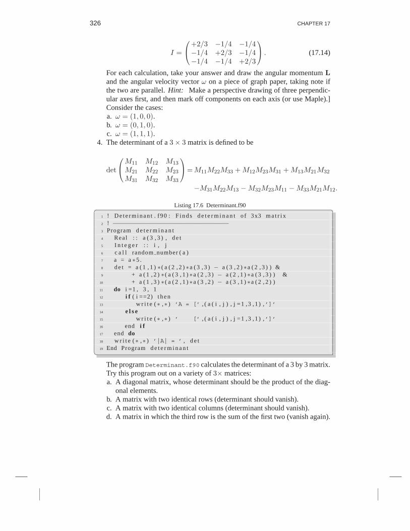
326 CHAPTER 17
I =
⎛⎝+2/3 −1/4 −1/4−1/4 +2/3 −1/4−1/4 −1/4 +2/3
⎞⎠ . (17.14)
For each calculation, take your answer and draw the angular momentum Land the angular velocity vector ω on a piece of graph paper, taking note ifthe two are parallel. Hint: Make a perspective drawing of three perpendic-ular axes first, and then mark off components on each axis (or use Maple).]Consider the cases:a. ω = (1, 0, 0).b. ω = (0, 1, 0).c. ω = (1, 1, 1).
4. The determinant of a 3× 3 matrix is defined to be
det
⎛⎝M11 M12 M13
M21 M22 M23
M31 M32 M33
⎞⎠=M11M22M33 + M12M23M31 + M13M21M32
−M31M22M13 −M32M23M11 −M33M21M12.
Listing 17.6 Determinant.f90
1 ! D e t e r m i n a n t . f90 : F i n d s d e t e r m i n a n t o f 3x3 m a t r i x2 ! −−−−−−−−−−−−−−−−−−−−−−−−−−−−−−−−3 Program d e t e r m i n a n t4 Rea l : : a ( 3 , 3 ) , d e t5 I n t e g e r : : i , j6 c a l l random number ( a )7 a = a ∗5 .8 d e t = a ( 1 , 1 ) ∗ ( a ( 2 , 2 ) ∗a ( 3 , 3 ) − a ( 3 , 2 ) ∗a ( 2 , 3 ) ) &9 + a ( 1 , 2 ) ∗ ( a ( 3 , 1 ) ∗a ( 2 , 3 ) − a ( 2 , 1 ) ∗a ( 3 , 3 ) ) &
10 + a ( 1 , 3 ) ∗ ( a ( 2 , 1 ) ∗a ( 3 , 2 ) − a ( 3 , 1 ) ∗a ( 2 , 2 ) )11 do i =1 , 3 , 112 i f ( i ==2) t h e n13 w r i t e (∗ ,∗ ) ’A = [’ , ( a ( i , j ) , j = 1 , 3 , 1 ) ,’]’14 e l s e15 w r i t e (∗ ,∗ ) ’ [’ , ( a ( i , j ) , j = 1 , 3 , 1 ) ,’]’16 end i f17 end do18 w r i t e (∗ ,∗ ) ’|A| = ’ , d e t19 End Program d e t e r m i n a n t
The program Determinant.f90 calculates the determinant of a 3 by 3 matrix.Try this program out on a variety of 3× matrices:a. A diagonal matrix, whose determinant should be the product of the diag-
onal elements.b. A matrix with two identical rows (determinant should vanish).c. A matrix with two identical columns (determinant should vanish).d. A matrix in which the third row is the sum of the first two (vanish again).

ARRAYS I: VECTORS, MATRICES; RIGID-BODY ROTATIONS 327
5. Here is the program ArrayTest.f90 that finds the maximum and minimumof a two-dimensional array of arbitrary length:
Listing 17.7 ArrayTest.f90
1 ! A r r a y T e s t . f90 : F ind min , max of 2D a r r a y2 ! −−−−−−−−−−−−−−−−−−−−−−−−−−−3 S u b r o u t i n e findMinMax ( x , min , max )4 I m p l i c i t None5 Real , d imens ion ( : , : ) , i n t e n t ( i n ) : : x6 Rea l : : min , max7 I n t e g e r : : i , j , imax , jmax8 imax = s i z e ( x , DIM=1) ;9 jmax = s i z e ( x , DIM=2) ;
10 min = x ( 1 , 1 )11 max = x ( 1 , 1 )12 do i =1 , imax , 113 do j =1 , jmax , 114 i f ( x ( i , j )<=min ) min = x ( i , j )15 i f ( x ( i , j )>=max ) max = x ( i , j )16 end do17 end do18 End S u b r o u t i n e findMinMax19 !20 Program main21 I m p l i c i t None22 I n t e r f a c e23 S u b r o u t i n e findMinMax ( x , min , max )24 Real , d imens ion ( : , : ) , i n t e n t ( i n ) : : x25 Rea l : : min , max26 I n t e g e r : : i , j , imax , jmax27 End S u b r o u t i n e findMinMax28 End I n t e r f a c e29 Rea l : : min , max , PI30 Real , d imens ion ( 1 0 , 1 0 ) : : a31 I n t e g e r : : i , j32 PI = 3 .14159265897933 ! I n i t i a l i z e t h e a r r a y34 do i =1 ,10 ,135 do j =1 ,10 ,136 a ( i , j ) = exp (−( i ∗ i + j ∗ j ) / 2 5 . 0 ) ∗ s i n ( ( i −1) &37 ∗PI / 7 ) ∗ cos ( ( j −1)∗PI / 5 )38 end do39 end do40 c a l l findMinMax ( a , min , max )41 w r i t e (∗ ,∗ ) ’Minimum = ’ , min , ’Maximum = ’ , max42 End Program main
a. Enter ArrayTest and get it running.b. Write a program ArraySort.f90 that uses ArrayTest to rearrange all the
elements of a 2D array from minimum to maximum values of the arrayelements. Here are some suggestions:

328 CHAPTER 17
•Use as much as you can of ArrayTest just to save yourself some typing.• The simplest, though not the most efficient, way to sort a list of numbersis to start with the first two elements, a[1] and a[2], interchange them ifa[1] is larger than a[2], and then go on to the next adjacent pair, a[2]and a[3], and perform the same operation. Continue until you get to theend of the array, a[n-1] and a[n]. While one pass through the array willnot be sufficient, n− 1 passes will.• Design a procedure that implements the sort procedure just described.While the program will turn out to be quite simple, it may take somethinking to get the logic thought through. Accordingly, first sketch out aflowchart or some pseudocode containing the key logical questions andconsequences. Hand in your design with the rest of your assignment.• Write a procedure xChange(a, i) that sorts a 2D array. To be safe, youmay want to read the discussion on changing an array element in the callto a procedure in § 17.5.

Chapter Eighteen
Advanced Function Methods, Objects*
In §16.5 we defined objects as non-primitive data types with multiple components.We have already used such objects to represent complex numbers and arrays, andhave investigated some of the interesting characteristics of employing objects asarray arguments. In this chapter we examine some more advanced use of proce-dures and objects.
18.1 PROCEDURE MODULES AND INTERFACES
The simple function and subroutine examples we have presented so far are all thata beginning user should need for their work. However, Fortran does permit somemore sophisticated techniques for dealing with procedures, and we shall discusssome of that now in the context of object-orientated programming (OOP). Whileincorporating these newer features in your programs does require some extra linesof code, OOP techniques lead to less-error prone programs, aid in debugging, andlead to more efficient compilation and optimization (speed) [F90 UL, ChapF 04].In addition to saving you time in the long run, we employ some of these techniquesin our examples, and so it is worthwhile for you to understand them somewhat.
Most of the procedures we have used as examples have been external. Thisis the older, Fortran77 approach in which each procedure is treated like a sepa-rate program unit that are developed and compiled independently from the mainprogram and the other procedures, and eventually linked together for execution.
In Fortran90, you may also group together user-defined data types and theprocedures that manipulate these types into modules. These modules are equiv-alent to what is called objects or classes in the Java and C++ programming lan-guages. Since an object is, in some sense, defined by the methods used to manip-ulate it, it makes sense to couple together new data types and the methods used tomanipulate them.
The real world often maintains some of the traditions of the past, and sosometimes you may need to include some already-written, tried-and-true, older
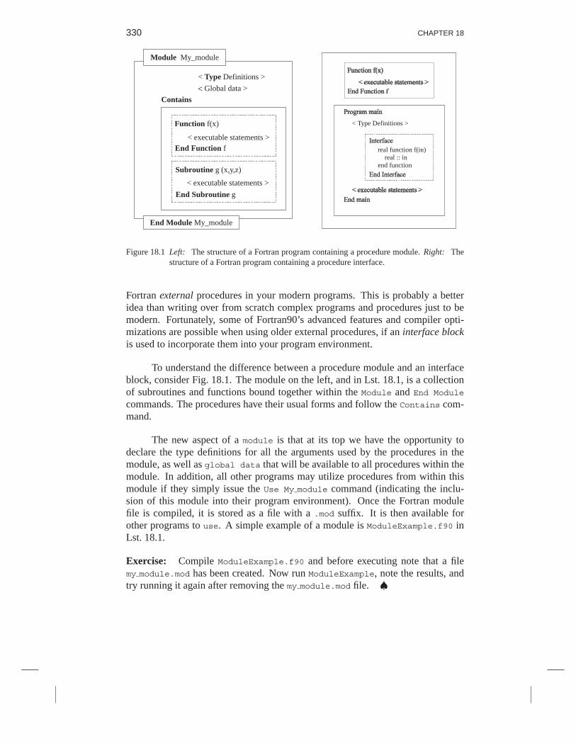
330 CHAPTER 18
Subroutine g (x,y,z)
< executable statements >
End Subroutine g
< executable statements >End Function f
Function f(x)
< Type Definitions >
< Global data >
Contains
Module My_module
End Module My_module
< Type Definitions >
real function f(in) real :: inend function
Figure 18.1 Left: The structure of a Fortran program containing a procedure module. Right: Thestructure of a Fortran program containing a procedure interface.
Fortran external procedures in your modern programs. This is probably a betteridea than writing over from scratch complex programs and procedures just to bemodern. Fortunately, some of Fortran90’s advanced features and compiler opti-mizations are possible when using older external procedures, if an interface blockis used to incorporate them into your program environment.
To understand the difference between a procedure module and an interfaceblock, consider Fig. 18.1. The module on the left, and in Lst. 18.1, is a collectionof subroutines and functions bound together within the Module and End Module
commands. The procedures have their usual forms and follow the Contains com-mand.
The new aspect of a module is that at its top we have the opportunity todeclare the type definitions for all the arguments used by the procedures in themodule, as well as global data that will be available to all procedures within themodule. In addition, all other programs may utilize procedures from within thismodule if they simply issue the Use My module command (indicating the inclu-sion of this module into their program environment). Once the Fortran modulefile is compiled, it is stored as a file with a .mod suffix. It is then available forother programs to use. A simple example of a module is ModuleExample.f90 inLst. 18.1.
Exercise: Compile ModuleExample.f90 and before executing note that a filemy module.mod has been created. Now run ModuleExample, note the results, andtry running it again after removing the my module.mod file. ♠

ADVANCED FUNCTION METHODS, OBJECTS* 331
Listing 18.1 ModuleExample.f90
1 ! ModuleExample . f90 : A module demo wi th a f u n c t i o n and s u b r o u t i n e2 ! −−−−−−−−−−−−−−−−−−−−−−−−−−−−−−−−−−−−−−−−−−−−3 Module my module4 C o n t a i n s5 Rea l ∗8 F u n c t i o n f ( x , y )6 I m p l i c i t None7 Rea l ∗8 : : x , y8 f = s i n ( x∗y ) + 1 . 09 End F u n c t i o n f
10 !11 S u b r o u t i n e f s u b ( x , y , c )12 I m p l i c i t None13 Rea l ∗8 : : x , y , c14 c = s i n ( x∗y ) + 1 . 015 End S u b r o u t i n e f s u b16 End Module17 ! −−− The main program t h a t u s e s t h e module18 Program main19 Use my module20 I m p l i c i t None21 Rea l ∗8 : : u =2 .1415 , v = 1 . , c22 c = f ( u , v )23 w r i t e (∗ ,∗ ) ’function’’s answer = ’ , c24 c a l l f s u b ( u , v , c )25 w r i t e (∗ ,∗ ) ’subroutine’’s answer = ’ , c26 End Program main
In contrast to a module, the interface block illustrated on the right ofFig. 18.1, and in Lst. 18.2, is only a block within the calling program that de-scribes the types and arguments of procedures to be called. The block is containedbetween the Interface and End Interface commands within the main program’sheader definitions. This block is not a separate entity that needs to be called, andit does not encapsulate the executable statements of the functions or subroutines(the two cannot be mixed in an interface). The interface block merely indicates tothe compiler which external procedures (and their types and arguments) are to beincluded in this program’s environment. Including those procedures in this wayallows for more complete error-checking.
So, even though a module is a preferable technique over an interface, thereare some circumstances when you might use an interface block to incorporatean existing, older procedure while still utilizing some of Fortran90’s advancedfeatures, as well as making it easier for the compiler to find errors or problems. Asimple example of an interface is FuncInterface.f90 in Lst. 18.2.
Exercise: Compile FuncInterface.f90, run it, and compare the results to theprevious example, ModuleExample.f90. ♠

332 CHAPTER 18
Listing 18.2 FuncInterface.f90
1 ! F u n c I n t e r f a c e . f90 : C a l l s a f u n c t i o n u t i l i z i n g an i n t e r f a c e2 ! −−−−−−−−−−−−−−−−−−−−−−−−−−−−−−−−−−−−−−−3 Rea l ∗8 F u n c t i o n f ( x , y )4 I m p l i c i t None5 Rea l ∗8 : : x , y6 f = s i n ( x∗y ) + 1 . 07 End F u n c t i o n f8 !9 Program main
10 I m p l i c i t None11 I n t e r f a c e12 Rea l F u n c t i o n f ( in1 , i n 2 )13 r e a l ∗8 : : in1 , i n 214 End F u n c t i o n f15 End I n t e r f a c e16 Rea l ∗8 : : i n 1 =2 .1415 , i n 2 = 1 . , c17 c = f ( in1 , i n 2 )18 w r i t e (∗ ,∗ ) ’function’’s answer = ’ , c19 End Program main
18.2 CHANGING THE ARGUMENTS OF A FUNCTION
Listing 18.3 Change.f90
1 ! Change . f90 : f u n c t i o n arguement change demo2 ! −−−−−−−−−−−−−−−−−−−−−−−−−−−−−−−−−−−−−−−−−3 Program change4 I m p l i c i t None5 I n t e g e r : : a =1 , b =2 , z , f6 w r i t e (∗ ,∗ ) ’In the main program, a =’ , a , ’, b =’ , b7 z = f ( a , b )8 w r i t e (∗ ,∗ ) ’In the main program, f(a,b) =’ , z , ’, then...’9 w r i t e (∗ ,∗ ) ’In the main program, a =’ , a , ’, b =’ , b
10 End Program change11 !12 I n t e g e r F u n c t i o n f ( x , y )13 I n t e g e r , i n t e n t ( i n o u t ) : : x , y14 x = 515 w r i t e (∗ ,∗ ) ’In the function, x =’ , x , ’, y =’ , y16 f = x + y17 End F u n c t i o n f
This is a warning of something that is more obvious with subroutines than withfunctions. When you call a function, the memory location of the argument ispassed to the function from the calling program. In other words, the main pro-gram sends only a memory reference or memory location to the function, not theactual value of the variable itself (the same as with arguments in subroutine calls).

ADVANCED FUNCTION METHODS, OBJECTS* 333
Accordingly, it is quite acceptable to call a function with the variable x as the argu-ment to the function, and then use a different variable like y for the correspondingvariable within the function itself. As a general rule, a function may change thevalue of its arguments, and those changes will be reflected in the correspondingvariables of the invoking routine. In other words, the changed value of the variablewill be returned to the calling program or procedure. Since we only concentrate onthe single value of the function name itself, we often do not think about this sideeffect.
The short program Change.f90 in Lst. 18.3 gives surprising results regard-ing the values of function arguments. To see them:
1. Compile and run Change.f90. You should get the results:In the main program, a = 1, b = 2
In the function, x = 5, y = 2
In the main program, f(a, b) = 7, then ...
In the main program, a = 5, b = 2
Look at the code and locate the four write statements. Compare them tothe printed results. Note that we start off with a = 1 and b = 2 in the mainprogram. Then the function f(a, b) is evaluated, where a and b are assignedto the variables x and y inside f . Inside f(x, y), the code sets x = 5,prints out the values (x = 5, y = 2), and returns a value of 7 for f. Whenwe get back to the main program, we print out f(a, b) = 7, and find thatthe assignment statement inside the function has caused the value of a in themain program to change!
What is happening here is that the variables in each function are localto that particular function and not “seen” by other parts of the program. Thevariables passed to the function f do not have their numerical values sent, butrather just their location in memory. Accordingly, the values for variables aand b in the main program are stored in the same memory locations as thevalues for variables x and y in the function f. If a is changed in f, then thecorresponding variable x will reflect that change in the main program. Sincememory locations, not values, are transferred between a calling program anda procedure, it is said that Fortran procedure calls call by reference ratherthan call by value.
2. Copy Change.f90 to Change2.f90. Modify the function declaration so thatthe arguments are reversed:
12. Integer Function f(y, x) Reversed arguments
Compile and execute Change2.f90. This program should convince you thatthe variable names inside a function are arbitrary and may be changed ac-cording to your preference, as long as the argument types still match. The

334 CHAPTER 18
function’s arguments are, after all, called “dummy” variables to indicate thatthey are only place holders.
3. As discussed before, you must always write your programs such that thearguments in the call to a function and in the function’s declaration matchexactly in type. So, for example, if a function is declared with the secondargument as a Real*8, then the calls to that function must have the secondargument as a Real*8, or else!. To see “or else what”, change the dummyarguments on line 12 to Real*8. Recompile Change.f90 and see the results.
4. Not only must the arguments of a function being called match the types ofthe function arguments declared by the function, but the value that the func-tion returns must also match the type declared for the function in the callingprogram. For example, make a working copy of Change.f90, and replacethe function declaration in on line 12 with one that declares the functionvalue returned to be a Real*8. Recompile Change.f90 and see the results.You should get an error message with a reference to “incompatible types”or “function result types differ.” These responses are signals of inconsistentdata types.
18.3 FUNCTIONS CALLING FUNCTIONS
So far, we have used the main program to call other functions. Actually, functionscan call other functions as well. Lst. 18.4 is an example that includes functionscalling other functions. Note that we are using double-precision variables and alsothe tangent function from the Fortran Math library.
Exercise: Compile and run Function3.f90. Compare the output you obtain withthe print lines in the code and explain why the results are as they are.
Listing 18.4 Function3.f90
1 ! F u n c t i o n 3 . f90 : Example o f f u n c t i o n s c a l l i n g f u n c t i o n s2 !−−−−−−−−−−−−−−−−−−−−−−−−−−−−−−−−−−−−−−−3 Module func modu le4 C o n t a i n s5 Rea l ∗8 F u n c t i o n f ( x , y )6 I m p l i c i t None7 Rea l ∗8 : : x , y , w8 w = g ( x ) ! c a l l t o f u n c t i o n g9 p r i n t ∗ , ’In f(x, y), x =’ , x , ’g(x) =’ , w
10 f = w ∗ w + y ∗ y ! c a l c u l a t e v a l u e f o r f11 End F u n c t i o n f12 Rea l ∗8 F u n c t i o n g ( x ) ! Module f u n c t i o n g13 I m p l i c i t None14 Rea l ∗8 : : x15 g = t a n ( x ) ∗∗ 3 ! use t a n f u n c t i o n f o r g16 End F u n c t i o n g17 End Module func modu le18 !

ADVANCED FUNCTION METHODS, OBJECTS* 335
19 Program main program20 Use func modu le ! I n c o r p o r a t e t h e module21 I m p l i c i t None22 Rea l ∗8 : : x = 1 . 0 , y = 3 . 0 , z23 p r i n t ∗ , ’In main, x =’ , x , ’y =’ , y24 z = f ( x , y ) ! c a l l t o f u n c t i o n f25 p r i n t ∗ , ’In main, f = ’ , z , ’x =’ , x , ’y =’ , y26 End Program main program
18.4 FUNCTION OVERLOADING
Now that we have warned you how important it is to have the data types of afunction’s arguments be the same in the calling program as it is in the functiondeclaration, we show you the exceptions to this rule. With function overloadingyou define a number of different functions having the same name but argumentsthat somehow differ. Explicitly, each function must have either 1) a different selec-tion of argument types, 2) a different number of arguments, or 3) a different returntype. You then can use the same function name for differing data types (with thehelp of the interface feature), and, incredibly enough, the compiler will choosethe proper one based on the unique combination of arguments and return type.While this may seem too forgiving, functions that differ only in return type are notacceptable.
Listing 18.5 Overload.f90
1 ! Over load . f90 : o v e r l o a d i n g v i a i n t e r f a c e2 ! −−−−−−−−−−−−−−−−−−−−−−−−−−−−−−−−−−−−−−−3 I n t e g e r F u n c t i o n f i n t ( i )4 I m p l i c i t None5 I n t e g e r : : i6 f i n t = i ∗ i7 End F u n c t i o n f i n t8 Rea l ∗8 F u n c t i o n f r e a l ( x )9 I m p l i c i t None
10 Rea l ∗8 : : x11 f r e a l = x∗x12 End F u n c t i o n f r e a l13 Complex∗16 F u n c t i o n f c o m p l e x ( z )14 I m p l i c i t None15 Complex∗16 : : z16 f c o m p l e x = z∗ c o n j g ( z )17 End F u n c t i o n f c o m p l e x18 !19 Program main20 I n t e r f a c e f21 I n t e g e r F u n c t i o n f i n t ( i )22 I n t e g e r : : i23 End F u n c t i o n f i n t24 Rea l ∗8 F u n c t i o n f r e a l ( x )

336 CHAPTER 18
25 Rea l ∗8 : : x26 End F u n c t i o n f r e a l27 Complex∗16 F u n c t i o n f c o m p l e x ( z )28 complex ∗16 : : z29 End F u n c t i o n f c o m p l e x30 End I n t e r f a c e f31 I n t e g e r : : a=232 Rea l ∗8 : : b =2 .33 Complex∗16 : : c = ( 1 . , 1 . )34 w r i t e (∗ ,∗ ) ’Integer: f(a) = ’ , f ( a )35 w r i t e (∗ ,∗ ) ’Real: f(b) = ’ , f ( b )36 w r i t e (∗ ,∗ ) ’Complex: f(c) = ’ , f ( c )37 End Program main
The program Overload.f90 in Lst. 18.5 is an example of overloading, usingan interface.
1. How many functions f do you see in this code?2. Compile and execute Overload.f90 to see function overloading in action.
Check that you get three lines of output and compare that output to the codeto ensure that three different functions with the same name were called.
3. Extend Overload.f90 so that it also calls a function f(x,y,z) where x, y,
and z are Real*8, as well as the function f(i,j,k), where i, j, and k areintegers.

Chapter Nineteen
Discrete Math, Arrays as Bins; Nonlinear Bug
Dynamics*
This chapter gives an example of how computations are used to model the pop-ulation dynamics of biological systems. It employs some fairly simple discretemathematics that leads to some unusual nonlinear behaviors to explore. One-dimensional arrays are used to bin store the results of the simulations, with thearrays then written to a file and visualized with Gnuplot. This chapter introducesno new Fortran tools, but instead reviews a number of previously introduced tech-niques. So even though there is no advanced material in it, we mark this chapteras optional since it may be skipped without interrupting the logical flow.
19.1 PROBLEM: VARIABILITY OF BUG POPULATIONS
As is true with much in nature, insect populations do not appear to follow anysimple patterns. At times they appear stable, at other times they vary periodically,and at still other times they appear chaotic, only to settle down to something simpleagain.1
Problem: Deduce and explore a simple model of the population as a function oftime that seems capable of producing complicated behaviors.
19.2 THEORY: SELF-LIMITING GROWTH, DISCRETE MAPS
Imagine a bunch of insects reproducing, generation after generation, in your gar-den. We start with N0 of them, in the next generation we have to live with N1
bugs, and after i generations there are Nn of them to bug us. We want a model forhow Nn varies with the discrete generation number n.
We look to the simple model of radioactive decay and growth for guidance.
1We actually use chaos as a technical term meaning complicated behavior in which there does not appear tobe any order, but in which there is some simple mathematical description [CP 05].
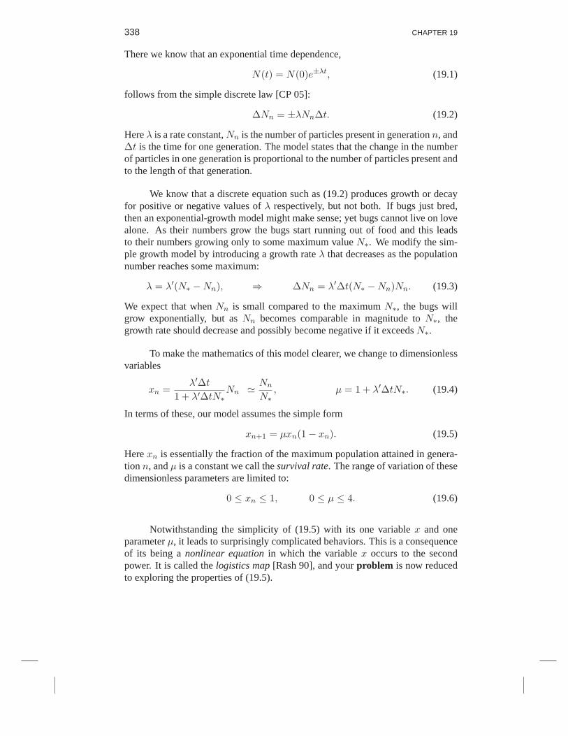
338 CHAPTER 19
There we know that an exponential time dependence,
N(t) = N(0)e±λt, (19.1)
follows from the simple discrete law [CP 05]:
∆Nn = ±λNn∆t. (19.2)
Here λ is a rate constant, Nn is the number of particles present in generation n, and∆t is the time for one generation. The model states that the change in the numberof particles in one generation is proportional to the number of particles present andto the length of that generation.
We know that a discrete equation such as (19.2) produces growth or decayfor positive or negative values of λ respectively, but not both. If bugs just bred,then an exponential-growth model might make sense; yet bugs cannot live on lovealone. As their numbers grow the bugs start running out of food and this leadsto their numbers growing only to some maximum value N∗. We modify the sim-ple growth model by introducing a growth rate λ that decreases as the populationnumber reaches some maximum:
λ = λ′(N∗ −Nn), ⇒ ∆Nn = λ′∆t(N∗ −Nn)Nn. (19.3)
We expect that when Nn is small compared to the maximum N∗, the bugs willgrow exponentially, but as Nn becomes comparable in magnitude to N∗, thegrowth rate should decrease and possibly become negative if it exceeds N∗.
To make the mathematics of this model clearer, we change to dimensionlessvariables
xn =λ′∆t
1 + λ′∆tN∗Nn Nn
N∗, µ = 1 + λ′∆tN∗. (19.4)
In terms of these, our model assumes the simple form
xn+1 = µxn(1− xn). (19.5)
Here xn is essentially the fraction of the maximum population attained in genera-tion n, and µ is a constant we call the survival rate. The range of variation of thesedimensionless parameters are limited to:
0 ≤ xn ≤ 1, 0 ≤ µ ≤ 4. (19.6)
Notwithstanding the simplicity of (19.5) with its one variable x and oneparameter µ, it leads to surprisingly complicated behaviors. This is a consequenceof its being a nonlinear equation in which the variable x occurs to the secondpower. It is called the logistics map [Rash 90], and your problem is now reducedto exploring the properties of (19.5).

DISCRETE MATH, ARRAYS AS BINS; NONLINEAR BUG DYNAMICS* 339
0 10 20 30n
0.0
0.2
0.4
0.6
0.8
1.0
xn
0 10 20 30n
0.0
0.2
0.4
0.6
0.8
1.0
xn
0 10 20 30n
0.0
0.2
0.4
0.6
0.8
1.0
xn
0 10 20 30n
0.0
0.2
0.4
0.6
0.8
1.0
xn
A B
C D
Figure 19.1 The insect population xn versus generation number n for various survival rates: (A)µ = 2.8, a period-one cycle; (B) µ = 3.3, a period-two cycle; (C) µ = 3.5, a period-four cycle; (D) µ = 3.8, a chaotic regime.
19.3 ASSESSMENT: PROPERTIES OF NONLINEAR MAPS
Rather than do some fancy mathematical analysis [Rash 90] to determine proper-ties of the logistics map (19.5), study it directly on the computer. Write a simpleprogram that uses the logistics map to produce a sequence of population values xnas a function of the generation number n. Start with a seed population x0 = 0.75and plot up xn versus n for µ = (0.4, 2.8, 3.3, 3.5, 3.8). The last four simulationsshould yield results similar to those in Figure 19.1.
Explore other nearby values of µ and identify on printed copies of yourgraphs the following characteristics:
Transients: Irregular behaviors before reaching a steady state.
Extinction: If the survival rate is too low, the population dies off.
Stable states: Single-population stable states for µ < 3.
Two and three cycles: At two-cycle fixed points, the population jumps back andforth between two semistable x∗ values. At three-cycle fixed points the population

340 CHAPTER 19
jumps between three x∗ values. These attractors occur only for µ > 3.
Intermittency: Try to find solutions for 3.8264 < µ < 3.8304 in which thesystem appears stable for a while but then jumps all around, only to become stableagain.
Chaos: The system’s behavior in the chaotic region is critically dependent on theexact value of µ and x0. Systems may start out much the same but end up quitedifferent. Compare the long-term behaviors of starting with the two essentiallyidentical seeds:
x0 = 0.75, x′0 = 0.75(1 + ε), (19.7)
where ε 2 × 10⁻¹⁴ for a double-precision calculation. Repeat the experimentwith x0 = 0.75, but with what should essentially be two identical survival para-meters:
µ = 4.0, µ′ = 4.0(1− ε). (19.8)
19.4 EXPLORATION: BIFURCATION DIAGRAM, BUGS.F90*
Listing 19.1 Bugs.f90
1 ! Bugs . f90 : B i f u r c a t i o n d iagram f o r l o g i s t i c map .2 ! bug p o p u l a t i o n − b i f u r c a t i o n map of m∗y∗(1−y )3 ! −−−−−−−−−−−−−−−−−−−−−−−−−−−−−−−−−−−−−−−−−−−−−4 Program Bugs5 I m p l i c i t none6 ! D e c l a r a t i o n s ( r a n g e and r e s o l u t i o n f o r m)7 Rea l ∗8 : : m min , m max , m, s t e p , y8 I n t e g e r : : x9 m min = 1 . 0
10 m max = 4 . 011 s t e p = 0 . 0 112 open ( 6 , F i l e =’bugs.dat’ , S t a t u s =’REPLACE’ )13 ! Loop f o r m v a l u e s , a r b i t r a r y s t a r t i n g v a l u e f o r y14 do m=m min , ( m max−s t e p ) , s t e p15 y = 0 . 516 ! Wait u n t i l t r a n s i e n t s d i e o u t17 do x =0 , 20018 y = m∗y ∗ (1 − y )19 end do20 ! Record 200 p o i n t s21 do x =201 , 40122 y=m∗y ∗ (1 − y )23 w r i t e ( 6 , 5 0 ) m, y24 end do25 end do26 c l o s e ( 6 , S t a t u s =’KEEP’ )27 ! Outpu t s t o r e d i n f i l e : bugs . d a t28 50 Format ( f5 . 3 , f10 . 6 )29 End Program Bugs

DISCRETE MATH, ARRAYS AS BINS; NONLINEAR BUG DYNAMICS* 341
1.0 2.0 3.0 4.0µ
0.0
0.2
0.4
0.6
0.8
1.0
xn
3.52 3.55 3.580.33
0.35
0.37
0.39
Figure 19.2 The bifurcation plot, attractor populations versus survival rate, for the logistics map.
Listing 19.1 gives our basic program for producing the data for a bifurcation dia-gram. Computing and watching the population change with each generation givesa good idea of the basic phenomena. However, it is hard to discern the simple andbeautiful behavior that lies within these complicated behaviors. One way to gainsuch understanding is to concentrate on the semistable population values x∗ thatthe system jumps among over time. These are called attractors to indicate that thesystem is somehow attracted to these populations.
A plot of these attractors as a function of the survival parameter µ is anelegant way to summarize the results of extensive computer simulations. One suchbifurcation diagram is given in Figure 19.2. It shows the output from the programBugSorted.java given here. For each value of µ, hundreds of iterations weremade to make sure that all transients died out. The value of x that the systemsettled down to is recorded as x∗. The doublet of points (µ, x∗) that occur after thetransients have died out were then written to a file. To be sure that all attractorshave been reached, the calculation is repeated for various values for the initialpopulations x0.
Implementation: Bifurcation Diagram
Create your own version of Figure 19.2 using Gnuplot. To get an idea of how manypoints may be needed, let us assume that your screen resolution is ∼100 dots perinch and that your laser printer’s resolution is ∼300 dots per inch. This means thatyou are plotting approximately 3000 × 3000 10 million elements. Beware: thiswill take a long time to print and require more memory than some printers haveavailable.

342 CHAPTER 19
Binning
1. Break up the range 1 ≤ µ ≤ 4 into 1,000 steps and loop through them. Theseare the “bins” into which we will place the x∗ values.
2. In order not to miss any structures in your bifurcation diagram, loop through arange of initial x0 values as well.
3. Wait at least 200 generations for the transients to die out, and then print out thenext several hundred values of (µ, x∗) to a file.
4. Print out your x∗ values to no more than three to four decimal places. You willnot be able to resolve more places than this on your plot, and this will keep youroutput files smaller by permitting you to remove duplicates2. Another approach isto remove two successive xn values that differ only beyond the third place. We dothat in the sample code Bugs.f90 by taking advantage of the fact that xn is in therange
0 ≤ xn ≤ 1. (19.9)
For this reason, before we write out to a file, we multiply our xn’s by 1,000, castthem as integers, and compare with the previous xn. If they are not equal, then weknow the xn value differs in the first three decimal places from the previous xnvalue.
5. Plot up your file of x∗ versus µ. Use small symbols for the points and do notconnect them.
6. Enlarge sections of your plot and notice that a similar bifurcation diagram tendsto be contained within portions of the original (this is called self-similarity).
7. Look over the series of bifurcations occurring at
µk 3, 3.449, 3.544, 3.5644, 3.5688, 3.569692, 3.56989, . . . . (19.10)
The end of this series is a region of chaotic behavior.
8. Inspect the way this and other sequences begin and then end in chaos. Thechanges sometimes occur quickly over a very short range of µ, and so you mayhave to make plots over a very small range of µ values to see the structures.
9. Close examination of Figure 19.2 shows regions where a very large number ofpopulations suddenly change to very few populations with a slight increase in µ.Whereas these may appear to be artifacts of the video display, this is a real effectand these regions are called windows. Check that at µ = 3.828427, chaos turnsinto a three-cycle population.
2For example, with the Unix command sort -u.

DISCRETE MATH, ARRAYS AS BINS; NONLINEAR BUG DYNAMICS* 343
Table 19.1 Maps for generating xn sequences and bifurcation plots.
Name f(x)
Logistics µx(1− x)
Tent µ(1− 2 |x− 1/2|)
Ecology xeµ(1−x)
Quartic µ[1− (2x− 1)4]
19.5 EXPLORATION: OTHER DISCRETE MAPS*
Only nonlinear systems exhibit unusual behavior like chaos. Yet systems are non-linear in any number of ways. Table 19.1 has maps that you may use to generatexn sequences and bifurcation plots.

Chapter Twenty
2-D Arrays: File I/O, PDE’s; Realistic Capacitor
The main purpose of this chapter is to get more experience with arrays, and espe-cially with the large 2-D ones used to solve realistic problems. As is often the casewith realistic problems, no analytic solution exists and we must employ a variety oftechniques to solve our problem. These include breaking space into a discrete lat-tice and applying a simple algorithm to solve a partial differential equation (PDE),file I/O, and 3-D visualization of numerical data using gnuplot. The simplicityof the solution follows from the use of large arrays that permit us to manipulatethousands or millions of variables with just a few lines of Fortran code.
20.1 PROBLEM: FIELD OF REALISTIC CAPACITOR
Figure 20.1, adapted from a first-year physics text, shows an idealized parallel-plate capacitor on the left. The equal spacing and single direction of the electric-field line (arrows) indicate that the field is uniform. On the right is a photograph ofthe electric field between the plates of a realistic parallel-plate capacitor, visualizedby small pieces of thread suspended in oil. Observe how the field fringes out nearthe ends and extends beyond the ends of the capacitor. Textbooks usually analyzethe ideal capacitor because only it can be treated analytically.
Problem: Determine and visualize the electric field within and surrounding arealistic capacitor, and compare to Figure 20.1.
20.2 THEORY AND MODEL: ELECTROSTATICS AND PDES
Capacitors are devices with the capacity to store electric charge. They usuallyconsists of two conductors of similar shape separated by a small gap, with equal—but opposite–charge on each conductor. Because the electric field, which wouldotherwise extend over all of space, is condensed to the region between the plates,capacitors are also called condensers.
In spite of real electrical devices being three-dimensional, we model thecapacitor, as shown on the left of Figure 20.2, as two wires connected to a battery

2-D ARRAYS: FILE I/O, PDE’S; REALISTIC CAPACITOR 345
V V−V −V
Figure 20.1 Left: Electric-field lines betweens the plates of an ideal parallel-plate capacitor. Theequal spacing and single direction indicate a uniform field. Right: A representationof the field between the plates of a realistic capacitor. The field tends to “fringe” andextend beyond the ends of the plates.
that keeps the top plate at 100 volts and the bottom one at -100 volts. To permita solution to this capacitor, we need to contain it in a limited space, which we doby placing it inside a charge-free box made from wires that are “grounded” (keptat 0 volts). After we solve this problem, we may make it more realistic still byenlarging the box so that it has no effect on the field near the capacitor. This islittle work for us, but much more work for the computer.
0V0
1020
3040
010
2030
40
- 100
- 50
0
50
100
x y
V(x,y )
100 V
- 100 V
Figure 20.2 Left: A parallel-plate capacitor within a grounded box. A realistic capacitor would havethe plates closer together in order to condense the field. Right: A visualization of theelectric potential for this geometry. The contours projected onto the xy plane give theequipotential surfaces.

346 CHAPTER 20
Laplace’s Partial Differential Equation*
Rather than solve for the electric field E(x, y), we solve for the electric potentialV (x, y). This is easier because V is a scalar while E is a vector, and because theequations for V are simpler. Insofar as the field E equals the derivative (gradient)of V , the two solutions are equivalent. (Electric-field lines are perpendicular toequipotential surfaces and run from higher to lower potential values.)
Elementary physics texts show how to determine electric-field configura-tions using Gauss’s law. We skip the mathematical manipulations needed to proveit and just state that the solution using Gauss’s law is equivalent to finding a solu-tion of the partial differential equation (PDE),
∂2V (x, y)∂x2
+∂2V (x, y)
∂y2= 0. (20.1)
This is called Laplace’s equation, in honor of the genius who first did those math-ematical manipulations. The rounded Ds in (20.1) indicate that the derivatives arepartial not ordinary. The reason this is a partial DE is that the potential functionV (x, y) is a function of both x and y. We cannot solve the x behavior withoutsimultaneously solving for the y behavior. The real world is full of such equations.
20.3 ALGORITHM: FINITE DIFFERENCES
The simplest method for solving our PDE is illustrated in Figure 20.3 and is knownas a finite-difference technique. There we see on the left a grid of x and y values,each uniformly spaced by a step size ∆x = ∆y = ∆. Rather than trying to find asolution for the continuous range of all possible values of x and y, we try to findthe solution only for the finite number of values that lie on the nodes of the grid.Yet even for the small 100 × 100 grid, this requires solving for 10,000 unknowns.Though not a trivial problem, the use of arrays makes it simple.
Approximating derivatives numerically is quite easy. In fact, in Chapter 15we show how to do it in order to find a solution of an ordinary differential equa-tion. In the present case, the second partial derivatives are approximated simply as[CP 05]:
∂2V (x, y)∂x2
V (x + ∆, y) + V (x−∆, y)− 2V (x, y)∆2
, (20.2)
∂2V (x, y)∂y2
V (x, y + ∆) + V (x, y −∆)− 2V (x, y)∆2
, (20.3)
where ∆ is the spacing of the grid in Figure 20.3. After we substitute this expres-sion, and the analogous one for the second y derivative, into Laplace’s equation

2-D ARRAYS: FILE I/O, PDE’S; REALISTIC CAPACITOR 347
Figure 20.3 Left: The capacitor’s field is computed only for those (x, y) values on the grid. Thevoltage of the plates and containing box are kept constant. Right: The algorithmfor Laplace’s equation in which the potential at the point (x, y) = (i, j)∆ equals theaverage of the potential values at the four nearest-neighbor points.
(20.1), we obtain a finite-difference approximation to the Laplace equation:
V (x, y) 14 [V (x + ∆, y) + V (x−∆, y) + V (x, y + ∆) + V (x, y −∆)] ,
V[i][j]= 14(V[i+1][j] + V[i-1][j] + V[i][j+1] + V[i][j-1]) . (20.4)
Equation (20.4) is the specific implementation of the equation we need to solvein terms of the 2-D Java array elements V[i][j] in which we store the potentialvalues for x = i∆ and y = j∆. This equation is visualized on the right ofFigure 20.3, which shows that the potential at point (i, j) is the average of thepotential values at the four nearest neighbors. If we wrote down this equationfor each of the 10,000 points on our grid, we would have 10,000 simultaneousequations for 10,000 simultaneous unknown values of Vi,j .
Even though it is possible to solve these 10,000 simultaneous equations ina direct fashion, we will follow a simple, indirect approach know as a relaxationtechnique. Equation (20.4) states that a solution for the potential must be the aver-age of the potential values at the four nearest neighbors. With that in mind, we tryan iterative approach to finding the solution:
1. Start with an initial guess V (x, y) = 0 every place except on the plates.2. To obtain an improved guess, apply (20.4) to all points in space, except the
plates and box.3. Keep applying (20.4) to obtain an even more approved guess until the im-
provement becomes smaller than some preset level of tolerance.
There is no guarantee that this relaxation method converges for arbitrary choices

348 CHAPTER 20
of ∆ and geometries. Yet if we do come up with a solution that ends up satisfying(20.4), then we have our solution and it’s nobody’s business how we got it!
20.4 IMPLEMENTATION: LAPLACEFILE.F90
Listing 20.1 LaplaceFile.f90
1 ! L a p l a c e F i l e . f90 : L a p l a c i a n e l e c t r o s t a t i c s on s q u a r e g r i d , F i l e2 ! −−−−−−−−−−−−−−−−−−−−−−−−−−−−−−−−−−−−−−−−−−−−−−−−3 S u b r o u t i n e s o l v e ( tmax , imax )4 I m p l i c i t None5 I n t e g e r , i n t e n t ( i n ) : : imax , tmax6 Real , d imens ion ( imax , imax ) : : V7 I n t e g e r : : i , j , k8 ! I n i t i a l i z e t h e m a t r i x V t o z e r o9 V=0 .
10 ! Boundary c o n d i t i o n s11 V( imax / 5 : 4 ∗ imax / 5 , imax / 3 ) = 1 0 0 . 012 V( imax / 5 : 4 ∗ imax / 5 , 2∗ imax / 3 ) = −100.013 V( 1 , 1 : imax ) = 0 . 014 V( imax , 1 : imax ) = 0 . 015 V( 1 : imax , 1 ) = 0 . 016 V( 1 : imax , imax ) = 0 . 017 ! J a c o b i r e l a x a t i o n18 do k =1 , tmax , 119 do i =2 , imax −1 ,120 do j =2 , imax −1 ,121 V( i , j ) = 0 . 2 5∗ (V( i +1 , j ) +V( i −1, j ) +V( i , j +1)+V( i , j −1) )22 ! C o n t i n u e a p p l y i n g i n t e r a l boundary c o n d i t i o n s23 i f ( j ==imax / 3 .AND. i >=imax / 5 .AND. i <=4∗imax / 5 ) t h e n24 V( i , j ) = 1 0 0 . 025 e l s e i f ( j ==2∗ imax / 3 .AND. i >=imax / 5 .AND. i <=4∗ imax / 5 )
t h e n26 V( i , j ) = −100.027 end i f28 end do29 end do30 end do31 ! Wr i t e t h e m a t r i x t o a f i l e32 open ( UNIT=1 , FILE=’LaplaceData.dat’ ,STATUS=’REPLACE’ )33 do i =1 , imax , 134 w r i t e ( 1 , 4 0 ) (V( i , j ) , j =1 , imax , 1 )35 w r i t e ( 1 , 5 0 )36 end do37 c l o s e ( UNIT=1 ,STATUS=’KEEP’ )38 40 f o r m a t (100 F13 . 6 )39 50 f o r m a t (’ ’ )40 End S u b r o u t i n e s o l v e41 !42 Program L a p l a c e F i l e43 I m p l i c i t None44 I n t e g e r : : tmax , imax

2-D ARRAYS: FILE I/O, PDE’S; REALISTIC CAPACITOR 349
45 imax =10146 tmax =100147 c a l l s o l v e ( tmax , imax )48 End Program L a p l a c e F i l e
We have prepared two implementations of our solution for a realistic ca-pacitor. The program LaplaceFile.f90, shown above in Lst. 20.1, solves theproblem and writes the solution to a file for separate visualization. The programLaplace.f90, given in Lst. 11.3 in Chapter11, solves the problem and then usesDislin to produce a 3-D visualization.
The pseudocode for our solution involves an outermost loop for iterations,and inner loops over imax x and y values:
1 s e t p o t e n t i a l = 0 on s u r r o u n d i n g around box2 s e t p o t e n t i a l = 100 , −100 on upper , p l a t e s3 r e p e a t 1000 t i m e s4 f o r imax x s p a c e s t e p s5 f o r imax y s p a c e s t e p s6 V = a v e r a g e o f 4 n e a r e s t n e i g h b o r s7 keep p o t e n t i a l on box and p l a t e s f i x e d8 w r i t e V m a t r i x t o a f i l e
This algorithm is well suited to the use of arrays because the indices vary,but not the equations. This means, as we see in Listing 20.1, that it does nottake too many lines of code to implement. We store the potential V (x, y) in anarray V(i,j), with the first index spanning all possible x values and the secondindex corresponding to all possible y values (measured in steps of ∆). The array isdeclared as V(imax,imax), and we set imax = 101 steps for the sample program.The voltages of the capacitor plates are kept fixed, while the boundary conditionsfor the box are imposed on lines 11-16.
The only tricky parts in LaplaceFile.f90 are ensuring that we do not letthe algorithm change the value of the externally-applied voltages, and that we dospecify any indices that lie outside of the array. Once there are no errors, we justlet the program repeat itself tmax=1001 times and relax into what we hope will bea stable value for the potential.
LaplaceFile.f90 Orientation and Visualization
Before trying to modify a complicated or subtle program, it is good to make surethat it runs, and to orient yourself as to how it goes about its business. Likewise,it is good to do some visualizations of the results so that you get a feel for what

350 CHAPTER 20
its output should be. For that purpose, make a copy LaplaceFile.f90 to yourpersonal directory and read through it to get a general idea of what it does.
• Make a paper listing of LaplaceFile.f90 and draw boxes on it illuminating thefollowing structures in the code:
1. the loop that initializes the potential to 0,2. the loop that keeps the box’s potential at 0,3. the loops that sets the voltage on the capacitor plates,4. the loops that sweep over all x and y values,5. the loop that implements the algorithm (20.4),6. the statements that output data to a file,
• Before you make any modifications, compile and execute LaplaceFile.f90.Make sure the data was indeed written to the file LaplaceData.dat. Open thefile LaplaceData.dat with an editor. It should contain the solution V (x, y) in aformat that does not bother telling you the x and y values. There are 100 valuesof V followed by a blank line. These are the values of V(1:100,0). The second100 numbers are V(1:100,1), and so forth. Note: The plotting program gnuplot
automatically uses the row and column indices as the values for x and y valuesthat it plots, which means that you do not have to enter them.
• Use gnuplot (or whatever you have available, such as Dislin) to construct a 3-Dsurface plots of the potential versus both x and y. Experiment with the optionsto create the best visualization. We show you how to do this with Gnuplot in§11.3, with the explicit command given in § 11.3. Your plot should look likeFigure 20.2. The height of the surface represents the value of the potential V (x, y)for the x and y values along the horizontal plane. Take stock of how the potentialof the bounding box is always zero, and that of the plates are 100 and -100 volts.On the horizontal plane we have placed contour lines that correspond to curvesalong which the potential is constant. These contours are also called equipotentialsurfaces. In general, the field is seen to be compressed between the plate and tovary more slowly outside the plates than within them.
• This program opens a file called UNIT=1, writes to it, and then closes the file.The REPLACE option on the open statement indicates that the old version of the filewill be written over, while the KEEP option on the close command ensures that thefile written to disk remains after the program stops executing.
20.5 EXPLORATION
• The program LaplaceFile.f90 assumes that the potential must have relaxed toits final value after 1000 iterations. Decide if this is a good assumption:

2-D ARRAYS: FILE I/O, PDE’S; REALISTIC CAPACITOR 351
Potential U(x,y) vs x and y
80 60 40 20 0
-20 -40 -60 -80
0 5 10 15 20 25 30 35 40 45 50
x Position
0
5
10
15
20
25
30
35
40
45
50
x Position
Figure 20.4 Contour plot of equipotential surfaces. The electric field lines are perpendicular to thesecontours and point toward lower potential.
a. Modify a copy of LaplaceFile.f90 so that it outputs to a file Laplace2.dat.b. Rather than try to discern small changes in a highly-compressed surface plot,
use a measure of precision with a numerical value. If you look at the surfaceplot of the potential in Figure 20.2, you will see that a line along the diagonalsamples the whole range of the potential. On this account, define a variable
trace =∑i
|V(i,i)| (20.5)
and print out the value of trace for each iteration. If trace changes in the sixthdecimal place, you probably have five good places of precision.
c. Now modify the program so that it always obtains at least three places ofprecision. Define tol = 0.001 as the desired relative precision and modifyLaplaceFile.f90 so that it stops iterating when the relative change from oneiteration to the next is less than tol:∣∣∣∣trace - traceOld
traceOld
∣∣∣∣ < tol. (20.6)
You can use a do-while loop for this purpose.
• Now that you know the code is accurate, make it simulate a more realistic capac-itor in which the plate separation is 1/10th of the plate length. You should find thefield more condensed between the plates.

352 CHAPTER 20
• Compare the results of your simulation to the sketch on the right of Figure 20.1.Whereas we are computing the electric potential while the sketch is of the electricfield, some processing is necessary. We make use of the fact that the electric fieldlines point from regions of higher to lower potential, and that the electric field linesare perpendicular to the equipotential surfaces (the contours in our plots). Thoughyou may try to draw lines perpendicular to the contours projected onto the base ofthe 3-D plot, it would be easier to look down directly onto the base. Make a 2-Dgraph, like Figure 20.4, of just the contour lines. The needed gnuplot commandsare gnu> set nosurfacegnu> set view 0,0,1
• Draw in the electric field lines by hand, starting from the plate at -100 volts,always keeping the field lines perpendicular to the equipotential surfaces and goingdownhill.
20.6 EXPLORATION: 3-D CAPACITOR*
Our solution for the capacitor is general and realistic. However, our model is onlytwo dimensional (the “plates” are lines not squares). Extend LaplaceFile.f90 sothat the plates have finite dimensions in both the x and y directions. You will nowhave to solve for V (x, y, z), and make three, 3-D surfaces of V (x, y, z) versusx− y, x− z, and y − z.
20.7 KEY WORDS
boundary conditions equipotential surfaces electric field electrostaticselectric potential equipotential lines capacitor gnuplothidden lines finite difference method initial conditions postscriptpartial derivatives reference pass contour lines

Chapter Twenty One
Web Computing (see Java Version)


PART 3
LATEX SURVIVAL GUIDE


Chapter Twenty Two
LATEX for Text: Scientific Document Processing,
Markup Language
22.1 WHY LATEX?
In the 1980’s Donald Knuth created a revolutionary computer program called TEX(“tech”) for producing book-quality technical documents [Knuth 86] that rivaledthe documents produced by a professional human typesetter. In 1985 Leslie Lam-port combined a number of TEX commands into a set of higher-level macrosknown as LATEX [Lap 85] that has fewer details to worry about than TEX. Atpresent LATEX is widely used for scientific journals, books, and reports, and forgood reason. LATEX automatically generates tables of contents, lists of figures,cross-references, equations, section and figure numbers, indexes, and bibliogra-phies. Nevertheless, it is the mathematics that LATEX does better than any otherelectronic system. This chapter describes enough of the basic elements of LATEX foryou to produce your own beautiful-looking scientific documents [Wilk 95].
To produce a LATEXdocument, all you have to do is prepare a source filewith some LATEX commands embedded at the correct places, and then compile thesource. Because the source file is an ASCII file, it is possible to write and read iton any computer system with no special programs. Of course one needs a copy ofthe LATEX program to typeset this ASCII file, but the program is free and readilyavailable.
The basic steps for using LATEX are shown in Figure 22.1. It is seen to bequite similar to compiling and running a code, and so makes a useful last part forthis book. By convention, the LATEX source file has a .tex extender and the com-piled version of the source has a .dvi extender. We have called our source filePaper.tex and the compiler has produced the device-independent file Paper.dvi
from it. A .dvi file is independent of any specific computer system or hardware,and is viewed on a computer screen with a program known as a viewer, or con-verted to a PostScript (.ps) or Portable Document Format (.pdf) file to be sent toa printer or posted on the Web.

358 CHAPTER 22
&'()))
*+
,)
-
Figure 22.1 The steps followed and utilities used in preparing a document with LATEX. The sourcefile is Paper.tex, the device-independent file is Paper.dvi, and the file ready forprinting/posting is Paper.ps or Paper.pdf.
The theory behind LATEX is that authors should worry about the contents of adocument and leave the format up to the computer. In practice there are a numberof steps to follow before authors see their documents typeset. This is in contrastto WYSIWYG (what you see is what you get), in which the formulas appear on thecomputer screen as you enter them. We personally prefer a markup-language ap-proach for complicated documents, especially if that document is to be placed in adigital library. We find that not having to concentrate on how things look until afterthe writing is over lets us get the hard part of creation done first. However, thereare a number of LATEX commands to learn, and debugging complicated equationscan be challenging. Nevertheless, a thing of beauty is a joy forever.
22.2 STRUCTURE OF A LATEX DOCUMENT
LATEX is a member of a class of languages known as markup languages.1 Theterm “markup” comes from the printing trade, where an editor would “markup” adocument by inserting symbols to indicate properties such as font size and spacing.This same purpose is served by the LATEX commands, only in this case they arenot for a human typesetter to follow, but for a computer. Inasmuch as LATEX isa compiled, in contrast to an interpreted, language, when you are done with thewriting, the compiler will read your entire document, place the tables, figures, andso forth, in the best places throughout your document, and then cross-reference thewhole thing. Like other compilers, you may have to remove all errors before thecompiler produces anything, and the compiler may need to make several passesthrough the document to get it all right.
22.3 SAMPLE INPUT FILE (SAMPLE.TEX)
A LATEX source file has two basic parts:
1Others include HTML, XML, GML, and MATHML.

LATEX FOR TEXT: SCIENTIFIC DOCUMENT PROCESSING, MARKUP LANGUAGE 359
1 \ d o c u m e n t c l a s s [ o p t i o n s ] c l a s s n a m e 2 . . .3 P a r t I : p reamble4 . . .5 \ b e g i n document6 . . .7 P a r t I I : a c t u a l document8 . . .9 %%\enddocument
The first part is the preamble, and it starts with a statement of the type of documentyour document is to be. The choices, classname = article, report, book,
slides, or letter, seem to cover most everything. Older versions of LATEX startedwith a \documenttype command, but the newer LATEX 2e uses the \documentclasscommand. The [options] argument might include the font sizes (in points)—10 pt (default), 11 pt, or 12 pt—as well as onecolumn (default), or twocolumn,oneside or twoside, or landscape. With \documentclassarticle you obtaina document in 10 pt font. The preamble might also include macros (commands)that you have defined for your own use, and commands for including special pack-ages, for example, for dealing with graphics.
To give you a real example, here, and on the CD is Sample.tex, an editedversion of a problem set with a comment following the %:
\documentclassarticle\begindocument
\sectionSample \LaTeX\ Output\indexComments!Latex@\LaTeX
\noindent This document consists of bits and pieces of afinal examination given at \textbf\large Oregon StateUniversity. The material is from the text\emphComputational Physics \citeCP, which does not costmuch \$\$.
We have left off anything fancy, like title page, from thepreamble and used an enumerated list environment(\tellenumerate), with mathematics environment inserted asneeded. An \emphEnvironment usually begins with\verb+\beginname+ and ends with \verb+\endname+.
% This is a one-line comment beginning with %; it does not get printed.
\beginenumerate
\item Given $N=6$ random numbers distributed between 0 and10,\[ 3, 7, 3, 1, 8, 2 \]
\beginenumerate\item Use this sequence to simulate a random walk and determine
if the distance from the origin $R = \sqrtN$.

360 CHAPTER 22
\item Use this sequence to determine an approximate value for thedouble integral
\beginequation\int_0ˆ1 \int_0ˆ1 dx\,dy\over xˆ2+yˆ2\endequation
\endenumerate
\item Given the Schr\"odinger equation for two coupledwave functions $\psi_1$ and $\psi_2$,
\begineqnarray-\hbarˆ2 \over 2m_1 dˆ2 \psi_1 (x)\over dxˆ2 + V(x)\psi_1(x) +
U(x)\psi_2(x) &=& E \psi_1(x) \labeleq.1 \\-\hbarˆ2 \over 2m_2 dˆ2 \psi_2 (x)\over dxˆ2 +V(x)\psi_2(x) +
U(x)\psi_1(x)&=& E \psi_2(x) \labeleq.2\endeqnarray
Express equations (\refeq.1) and (\refeq.2) in thedynamical form appropriate for numerical integration:\[d \textbfy(t)\over dt = \textbff(y,t)\]\endenumerate%\enddocument
When we apply LATEX to these paragraphs we produce the text:
22.4 SAMPLE LATEX OUTPUT
This document consists of bits and pieces of a final examination given at Oregon State University.The material is from the text Computational Physics [CP 05], which does not cost much $$.
We have left off anything fancy, like title page, from the preamble and used an enumerated list environ-ment (enumerate), with mathematics environment inserted as needed. An Environment usually begins with\beginnameand ends with \endname.
i) Given N = 6 random numbers distributed between 0 and 10,
3, 7, 3, 1, 8, 2
(a) Use this sequence to simulate a random walk and determine if the distance from the origin R =√N .
(b) Use this sequence to determine an approximate value for the double integral∫ 1
0
∫ 1
0
dx dy
x2 + y2(22.1)
ii) Given the Schrodinger equation for two coupled wave functions ψ1 and ψ2,
−h2
2m1
d2ψ1(x)
dx2+ V (x)ψ1(x) + U(x)ψ2(x)=Eψ1(x) (22.2)
−h2
2m2
d2ψ2(x)
dx2+ V (x)ψ2(x) + U(x)ψ1(x)=Eψ2(x) (22.3)
Express equations (22.2) and (22.3) in the dynamical form appropriate for numerical integration:
dy(t)
dt= f(y, t)

LATEX FOR TEXT: SCIENTIFIC DOCUMENT PROCESSING, MARKUP LANGUAGE 361
Brief Look at Input File
Most of the characters in our input file Sample.tex are the same as in the output.However, mathematical symbols, Greek, and some special characters are enteredwith commands: the math symbols and Greek, because they do not appear onthe keyboard, the special characters because LATEX uses them within its own com-mands.
Look at the commands in Sample.tex. You will notice that LATEX commandsusually consist of a backslash \ followed by a word. As an instance, we use \item,\beginequation, and \emphComputation Physics respectively. The Greekletter ψ was produced with \psi, and the mathematical symbol
√N with \sqrtN.
As we also see in these examples, the special characters and are used toenclose the argument to a LATEX command. To illustrate, the √ is applied to Nvia \sqrtN, and both the words Computational and Physics are emphasized by\emphComputational Physics. Of special importance in this file is the dollarsign $. When used as part of the text to indicate a dollar sign, it is entered as \$.When used as part of LATEX command to switch between text and math modes, itis entered as $, for example:
coupled wave functions $\psi_1$ and $\psi_2$ coupled wave functions ψ1 and ψ2
Although we talk more about this in a separate section, we produced math-ematical equations that were separated off from the text (“displayed”) by plac-ing them between the commands \[ and \], or between \beginequation and\endequation, or between \begineqnarray and \endeqnarray.
Special Characters
The characters
# $ % & ˜ ˆ \
are called “special characters” because LATEX uses them for its own purposes. Thismeans that you cannot use them unless you do something special. If you simplywant the special character to be printed just as any other letter, include a \ in frontof the character:
$ \$
There are two exceptions to this rule. You cannot produce \ via \\, becauseLATEX uses \\ to indicate the end of a line. So produce it by typing $\backslash$:
\ $\backslash$

362 CHAPTER 22
The second exception is the tilde. Seeing that \˜ means “place a tilde accent overthe following letter,” a ˜ is produced by \˜, that is, having nothing there (emptybraces) for the tilde to go over:
˜name \˜name
Paragraphs, Spaces, and Breaks
Look now at the two short paragraphs below the headings in Sample.tex. A newparagraph is indicated by one (or more) skipped lines. LATEX then automaticallyindents the paragraph as appropriate for its place in the document, for example, itdoes not indent at the beginning of a new section. To ensure that our first paragraphafter the table is not indented, we placed a \noindent command there.
Ordinary text is entered with no special commands. In general you do noteven have to worry about the spacing between words and lines, or where linesbegin and end. LATEX treats any number of spaces as equivalent to a single space,and views the carriage return ( Enter) at the end of a line as though it were justanother space. If you want to insist on an extra blank space being inserted at somepoint, then you insert a \ command, that is, a blank space preceded by a backslash.This means that you do not have to worry about spaces in your input, although youshould give it some structure with spaces and new lines to make the content clear,as you would with any coding.
Though you should not have to do this for most of your work, sometimesyou do need to insert a horizontal or vertical blank space in your document. Yourequest that LATEX does that (a “request” because LATEX has its own ideas aboutspacing, and it gets the last word) with the \hspace and \vspace commands.You become more insistent by using the \hspace* and \vspace* forms. Thesecommands take the length of the space as an argument in the braces. The length isspecified with a number of dimensional units that include:
ex em pt pc in cm mm
Here, ex and em are the sizes of a typeset x and m, pt and pc are the typesettingmeasures of points and picas, and the others are obvious.
Here is a 4ex horizontal space. Here \hspace4ex is a 4ex horizontal space.
Here is a 9mm horizontal space. Here \hspace9mm is a 9mm horizontal space.
Negative space & overstriking— Negative space & overstriking\hspace-3em---
A 3ex vertical space between here A 3ex vertical space between here \vspace3ex
and this line. and this line.

LATEX FOR TEXT: SCIENTIFIC DOCUMENT PROCESSING, MARKUP LANGUAGE 363
If you want to insist on a line ending someplace and a new paragraph begin-ning, then you insert a double backslash \\ to end the line. In addition, you addsome extra blank space after the line by including an argument to \\. To illustrate,we place \\*[3ex] here,
and you see that it skips three ex’s of space before printing this line.
Usually LATEX decides where to start a new page according to its own internalrules. As an example, it tries not to split up tables or place the last line of aparagraph on a new page. If you disagree with LATEX’s decision and wish to forcea page break, use:
\pagebreak hint to LATEX if embedded, command if on separate line\newpage, \clearpage no attempt to fill page
Though you would never “double-space” a book or journal article, thereare occasions when you want to double-space a draft, or to make a business let-ter fill the page. If you want to vary the interline spacing, you need to changethe LATEX environmental variable \baselinestretch from its default value of 1.Generally you do this in the preamble with:
\renewcommand\baselinestretch1.75
where we have set the spacing to one and three-quarter lines. The command thenholds for the entire document. (You may try to reset the spacing locally, but thatmay mess up the length of the page.)
Quotation Marks and Dashes
Despite most of us never worrying about such things, LATEX is fairly serious whenit comes to quotation marks and dashes. This is a consequence of its being atypesetting program, and typesetters are very serious about such things. Whenwriting in LATEX , we usually place a word in quotation by placing two left quoteson the left side and two right quotes on the right. As a case in point, the quotes in
“golfballs appear to ‘drop out of the sky’ near the end of their trajectories”
is produced from the input
‘‘golfballs appear to ‘drop out of the sky’ near the end oftheir trajectories’’
Scrutinize how the left double quote “ is entered as two left single quotes in succes-

364 CHAPTER 22
sion, ‘ and ‘, and the right double quote is entered as two right single quotes, ’ and’. As a general rule, one should not use the (undirected) ‘double quote’ character" on the keyboard. (Some text editors, like emacs, automatically substitute either“ or ” when you enter " if they know you are entering a LATEX document.)
LATEX and typesetters deal with dashes of three lengths:
intra-word dash or hyphen, as in intra-word intra-word dash or hyphen, as in intra-word
double dash indicates range, as in 3–8 double dash indicates range, as in 3--8
triple or punctuation dash—popular in news triple or punctuation dash---popular in news
22.5 FONTS FOR TEXT
The basic theory behind LATEX is that the user should worry about content andlet the program worry about presentation. So it follows that you should tellLATEX whether you want some material to be emphasized, or emboldened, orpresented as mathematics, but you should not have to worry about the name orsize of the actual font being used. To give an instance, you emphasize text, andLATEX usually reacts by placing that text in italic font. However, LATEX uses a dif-ferent italic font for text than it does for mathematics; for example, this (math)is different from this (text).
By default, LATEX uses the Computer Modern fonts, which give a character-istic look to LATEX documents. If you really want some material to have a certainpresentation that differs from LATEX’s standard, then you may have to change somethings “by hand” or develop some macros. However, those occasions should berare and should be done only at the last minute before final presentation. Thewords you wish to have in a specific format are usually given as the arguments, forexample:
Emphasized text \emphEmphasized text
Bold text \textbfBold text
Teletype (monospaced) text \textttTeletype (monospaced) text
SMALL CAPITAL LETTERS \textscsmall capital letters
f = md2x/dt2 (math) $f = m dˆ2 x/dtˆ2$ (math)
Explicit fonts are obtained with commands of the sort:
Roman font \textrmRoman font
Italic font \textitItalic font
Sans serif font \textsf\small Sans serif font
Slanted, but not italics \textslSlanted, but not italics
If you are working with someone else’s document, you may run into some old stylecommands for font changes. Though not strictly LATEX 2e, these still work:

LATEX FOR TEXT: SCIENTIFIC DOCUMENT PROCESSING, MARKUP LANGUAGE 365
Emphasized \em Emphasized
Bold \bf Bold
Teletype \tt Teletype
Type Sizes
I’m tiny \tinyI’m tiny I’m scriptsize \scriptsizeI’m scriptsize
I’m footnotesize \footnotesizeI’m footnotesize I’m small \smallI’m small
I’m normalsize \normalsizeI’m normalsize I’m large \largeI’m large
I’m Large \LargeI’m Large I’m LARGE \LARGEI’m LARGE
I’m huge \hugeI’m huge I’m Huge \HugeI’m Huge
Fancy Text Accents
English appears to be an underachiever when it comes to accents. However, ifyou wish to include some foreign text in your documents, then you may well needsome of the accents LATEX provides:
\’o o \‘o o \ˆo o \"o o \˜o o \=o o\.o o \uo o \vo o \Ho o \too oo \co o\do o. \bo o
¯\’i ı \’j j
If you want to accent mathematics, then different commands are needed yet, andwe will get to that.
Math Symbols in Text
Placing mathematics in text, such as∫f(x)dx, is done by placing the mathematics
between dollar signs, for example, $\int f(x)dx$. Other symbols are created inmath mode with the commands:
# \# $ \$ % \% & \&
\ $\backslash$ \ \verb’\’ ˆ \verb’ˆ’ ˆ \char94
ˆ \ˆ ˜ \char126 \ \
\_ œ, Œ \oe, \OE æ, Æ \ae, \AE ra, rA \aa, \AA
ω, Ω \o, \O ł, Ł \l, \L ß \ss ¿ ?‘
¡ !‘ † \dag ‡ \ddag § \S
P \P c© \copyright £ \pounds

366 CHAPTER 22
22.6 ENVIRONMENTS
A LATEX Environment usually begins with \beginname and ends with\endname. Indeed, since a LATEX document begins and ends as\begindocument . . . \enddocument, the entire source file is in a docu-ment environment. Other environments include:
array math arrays center centered text or tablesdescription definition list document the full LATEX documentenumerate numbered and lettered list eqnarray aligned equationsfigure floating figure itemize bullet listlist custom list minipage page within a pagepicture basic diagram drawn by LATEX quotation long quotationquote short quotation tabbing define and use tabstable floating and referenced table tabular in-place tableverbatim set as entered in \texttt \verb|text| in-line verbatim
22.7 LISTS
LATEX supports three types of lists:
enumerate: for numbered lists;
itemize: for bullet lists;
description: for definition lists like this;
list: custom lists.
\LaTeX supports three types of lists:\begindescription\item [enumerate] for numbered lists, \item [itemize ] forbullet lists, \item [description ] for definition lists likethis. \item [list ] Custom lists\enddescription\endenumerate
The numbers or bullets are provided automatically by LATEX , so all the user has todo is separate items by an \item command:
1. This is a numbered list, but you need not enter numbers.2. This second item contains math sin2 x + cos2 x = 1.
\beginenumerate\item This is a numbered list, but no numbers are entered.\item This second item contains math $\sinˆ2 x+\cosˆ2 x =1$.\endenumerate

LATEX FOR TEXT: SCIENTIFIC DOCUMENT PROCESSING, MARKUP LANGUAGE 367
Sublists are created just by starting another list within an existing list.LATEX generates yet different symbols for sublists:
1. First item in lista. First item in sublistb. Second item in sublist
2. Second item in list
\beginenumerate\item First item in list
\beginenumerate\item First item in sublist\item Second item in sublist\endenumerate
\item Second item in list\endenumerate
Text Tables
Tables are produced in the LATEX text mode by entering the tabular environment.It is entered via \begintabular..., and exited via \endtabular. The tableis placed in the text at the location in which it is entered. If you want a table thatis numbered, that has a caption, and that can be referenced, then you insert your\tabular commands between a set of \table commands. We describe that later.
Here is a table from one of our Java chapters:
Description Data Types Size Examples
single character char 2B a, e, I, $, 6integer byte, short, int, long 1, 2, 4, 8 B 12, -30, -128, 127floating point float, double 4, 8 B 9.34F, 7.2867logical boolean (≤,≥) 1 bit true or false
It is the result of:
\begintabular|l||c|c|r|\hline\hline \textbfDescription & \textbfData Types &\textbfSize & \textbfExamples \\*[2ex] \hlinesingle character & \tellchar & 2B & a, e, I, \$, 6 \\integer & \tellbyte, short, int, long & 1, 2, 4, 8 B & 12, -30, -128, 127\\floating point & \tellfloat, double & 4, 8 B & 9.34F, 7.2867\\logical & \tellboolean ($\leq,\geq$) & 1 bit&true or false\\\hline\endtabular
The argument in braces after the \begintabular command specifies the formatfor the columns in the table. The l indicates that the first column is left-justified.

368 CHAPTER 22
The two c’s indicates that the next two columns are centered, and the last r in-dicates that the fourth column is right-justified. The vertical bars | are optionaland instruct LATEX to place vertical bars in the columns indicated. The fact that wehave bars before the first column and after the last means that we want bars on theoutsides of the table.
Peer at how we have two \hline commands before we enter the data, asingle \hline command after we enter the column headings, and a single \hline
command after we have entered all the data. These commands cause the horizontallines in the table to be drawn. They too are optional and must be placed after arow separator \\ or before the rows begin.
Data are entered into the table one row at a time. Each row ends with adouble backslash \\, and the columns are separated by an ampersand character &.Mathematical symbols or equations are placed in the table by switching to mathmode, which we did with ≤ and ≥.
You do not have to specify the number of rows in your tables; LATEX willknow when you are done from the \endtabular command. In the present exam-ple we end the last row with a \\. Normally that is not necessary, but we includeit because we have a \hline command to follow. If you need some more verticalspace between two rows, include a space option such as \\*[2ex] to end a row.We did that after the heading.
Floating Tables
In published books and journals, tables and figures often “float” on the page. Thismeans that they are placed where they fit in best, which is often not at the placewhere they are first mentioned. Clearly, this becomes more important as your tableor figure gets larger and harder to fit in someplace. Table 22.1 is an example of afloating table. It is produced with the commands:
\begintable\captionA sample floating table with a number and a caption.\begintabular|c|ccc|c|\hline\hlineBinary $abc$ & $= a\times 2ˆ2$ & $+ b\times2ˆ1$ & $+c \times 2ˆ0$ & = Decimal \\\hline000 & 0 & 0 & 0 & 0\\001 & 0 & 0 & 1 & 1\\010 & 0 & 1 & 0 & 2\\111 & 1 & 1 & 1 & 7\\ \hline\endtabular\labeltab.binary2\endtable

LATEX FOR TEXT: SCIENTIFIC DOCUMENT PROCESSING, MARKUP LANGUAGE 369
Table 22.1 A sample floating table with a number and a caption.
Binary abc = a× 22 +b× 21 +c× 20 = Decimal000 0 0 0 0001 0 0 1 1010 0 1 0 2111 1 1 1 7
Inspect how the table is made by inserting the standard \begintabular and\endtabular pair within a \begintable and \endtable pair. In addition,there are \caption and \label commands within the table environment butoutside of the tabular environment. The argument to \caption contains the captionthat appears under the table. (If the caption command appears before the tabularcommand, the caption will be above the table.) The argument to \label is a tagthat is used to reference the table with the \ref command (the numbering is doneautomatically):
Table 22.1 is referenced Table˜\reftab.binary2 is referenced
This same scheme of labeling and referencing is used with equations.
22.8 SECTIONS
and
Subsections
and
Subsubsections
LATEX permits you to have sections, subsections, and subsubsections in your doc-uments. You give each a title, and LATEX gives each a sequential number, whichchanges automatically as other sections are inserted or removed, and a differentsized heading. By way of example, the section, subsection, and subsubsectionright above this paragraph were produced with the commands:
\sectionSections and \subsectionSubsections and \subsubsectionSubsubsections

370 CHAPTER 22
Placing an asterisk before the title of the section or subsection will suppressLATEX ’s automatic numbering, as in \section*A Section without a Number.
Quotations and Footnotes
LATEX contains two commands for setting off text from its surroundings. The quoteenvironment is used for short quotations, while the quotation environment is ap-propriate for longer ones. They differ in indentation:
This is a quote. Look at how this first paragraph is indented. Thequote environment is used for short quotations.
This is still the quote Observe how this second paragraph is indented.To repeat, a quote environment is for short quotations.
This is a quotation. Observe how this first paragraph is indented.The quotation environment is appropriate for longer quotations.
This is still the quotation. Check how this second paragraph is in-dented and spaced. A quotation environment is for longer quotations.
\beginquote ... \endquote
\beginquotation ... \endquotation.
Footnotes are created with the \footnotetext command. You place thecommand where you want a reference to the footnote, and LATEX automaticallyplaces a reference there and sets the note at the bottom of the page. For instance,we place a footnote here2 with \footnoteSample note with its own period..You should find it below and below a horizontal line.
2Sample note with its own period.
Chapter Twenty Three
LATEX for Mathematics
23.1 ENTERING MATHEMATICS: MATH MODE
Typesetting mathematics properly is a challenge for humans and their computercounterparts. In order for mathematical symbols to convey their meanings prop-erly, their size and vertical and horizontal placements must adhere exactly to ac-cepted mathematical notation. LATEX does a beautiful job at mathematical type-setting, better than any other program, in our opinion, and is almost as good as ahuman typesetter.
To input an equation or mathematical symbol you enter math mode, andthen leave math mode when you want to enter text again. The equations or sym-bols may be embedded in text or displayed (set off) between lines of text. In-textmathematics, such as R =
√N , is surrounded by dollar signs $R = \sqrtN$, the
first one indicating a switch from text to math mode, the second one indicating aswitch back from math to text:
R varies as R ∝√N for $R$ varies as $R \propto \sqrtN$ for
In addition to dollar signs, you may also use \( and \) to mark the beginning andthe end of a mathematical formula or symbol embedded in text:
R varies as R ∝√N \(R\) varies as \(R \propto \sqrtN\)
Though probably just a matter of taste, we find it easier to read and edit aLATEX source file when there are dollar signs in the text; to us, the \( and \) looktoo much like part of the equation.
Mathematics that is displayed (separated from the text) looks like:
−h2
2md2ψ(x)dx2
+ V (x)ψ(x) = Eψ(x). (23.1)
Check that this equation has a number on the extreme right (automatically assignedby LATEX) and a period for punctuation (put there because we prefer equations with
372 CHAPTER 23
punctuation). This equation was obtained with the LATEX input:
\beginequation-\hbarˆ2 \over 2m dˆ2 \psi (x)\over dxˆ2 + V(x)\psi(x) = E \psi(x).
\endequation
The \beginequation and \endequation commands define the environment fornumbered mathematical equations. If you do not want the equation to be num-bered, that is, so it appears as:
−h2
2md2ψ(x)dx2
+ V (x)ψ(x) = Eψ(x),
then use \[ and \] to begin and end the displayed equation environment:
\[-\hbarˆ2 \over 2m dˆ2 \psi (x)\over dxˆ2 + V(x)\psi(x) = E \psi(x).
\]
23.2 MATHEMATICAL SYMBOLS AND GREEK
Most characters have their standard meaning in math mode. However, letters usedas symbols appear in a special mode of italic, and function names and subscriptsappear in Roman. The special characters, already discussed in §22.3, are enteredin math mode as:
# \# $ \$ % \% & \& \_ \ \ \ \backslash
The spacings between math symbols will be different than the spacings in textmode and are designed to make the mathematics clearer. As always, LATEX ignoresextra spaces or carriage returns in the your source file, unless you force the issue.This means that you may insert extra spaces in your source file for clarity, ordistribute your equations over several lines. LATEX will put it all together and makeit look nice. If you insist on inserting spaces (not worth the trouble unless you arepublishing the document). For example, if you enter $xy$you get xy, otherwise:
x y x\ y normal space x y x\:y medium space x y x\,y thin spacex y x\;y thick space xy x\!y back space x y x\ \ y double space
Greek Letters
Greek letters are produced in math mode by preceding the full name of the letterby a backslash \. For example, C = 2πr is input as $C = 2 \pi r$. The lowercaseGreek letters are obtained as:

LATEX FOR MATHEMATICS 373
α \alpha β \beta γ \gamma δ \delta ε \epsilon
ε \varepsilon ζ \zeta η \eta θ \theta ϑ \vartheta
ι \iota κ \kappa λ \lambda µ \mu ν \nu
ξ \xi o o (text o) π \pi ρ \rho \varrho
σ \sigma ς \varsigma τ \tau υ \upsilon φ \phi
ϕ \varphi χ \chi ψ \psi ω \omega
For those that are different from their Roman counterparts, uppercase Greek lettersare obtained by capitalizing the first character of their names:
Γ \Gamma ∆ \Delta Θ \Theta Λ \Lambda Ξ \Xi Π \Pi
R R (text R) Σ \Sigma Υ \Upsilon Φ \Phi Ψ \Psi Ω \Omega
Relations
≤ \leq ≤ \le ≥ \geq ≥ \ge ≡ \equiv
≺ \prec \succ ∼ \sim \preceq \succeq
\simeq \ll \gg \asymp ⊂ \subset
⊃ \supset ≈ \approx ⊆ \subseteq ⊇ \supseteq ∼= \cong
\sqsubseteq \sqsupseteq \bowtie ∈ \in \ni
\owns ∝ \propto \vdash ! \dashv |= \models
! \smile | \mid | \vert.= \doteq " \frown
‖ \parallel ‖ \Vert ⊥ \perp : \colon ∧ \wedge
∧ \land ∨ \vee ∨ \lor · · · \cdots . . . ldots
Negative Relations
Most negative relations are formed by including a \not command in front of thenormal relation:
≤ \not\leq ≡ \not\equiv
This is just \not placed in front of \leq and \equiv. In addition, the symbol = maybe formed in a number of ways:
= \neq \ne \not\equal

374 CHAPTER 23
Binary (and Other) Operators
± \pm ∩ \cap ∨ \vee ∓ \mp ∪ \cup
∧ \wedge \ \setminus ) \uplus ⊕ \oplus · \cdot
+ \sqcap , \sqcap × \times - \sqcup ⊗ \otimes
∗ \ast \triangleleft / \oslash # \star \triangleright
0 \odot 1 \diamond 2 \wr † \dagger \circ
© \bigcirc ‡ \ddagger • \bullet 4 \bigtriangleup 5 \amalg
÷ \div 6 \bigtriangledown
Arrows
← \leftarrow → \rightarrow ←− \longleftarrow−→ \longrightarrow ⇐ \Leftarrow ⇒ \Rightarrow⇐= \Longleftarrow =⇒ \Longrightarrow ↔ \leftrightarrow⇔ \Leftrightarrow \swarrow ⇐⇒ \Longleftrightarrow← \hookleftarrow → \hookrightarrow \leftharpoonup \rightharpoonup \leftharpoondown ↓ \downarrow↑ \uparrow \rightharpoondown ⇑ \Uparrow⇓ \Downarrow \updownarrow \Updownarrow \nearrow \nwarrow \searrow←→ \longleftrightarrow → \mapsto −→ \longmapsto
Math Parentheses
[ \lbrack ] \rbrack 7 \lfloor 8 \rfloor 9 \lceil : \rceil
\lbrace \rbrace 〈 \langle 〉 \rangle \ (alt) \ (alt)
Miscellaneous Math Symbols
ℵ \aleph ′ \prime ∀ \forall h \hbar ∅ \emptyset∃ \exists ı \imath ∇ \nabla ¬ \neg j \jmath√
\surd ⊥ \bot \ell \top \natural℘ \wp \flat \sharp \angle ‖ \|! \triangle Im \Im Re \Re \backslash ∂ \partial
\clubsuit ♥ \heartsuit ♠ \spadesuit ♦ \diamondsuit ∞ \infty

LATEX FOR MATHEMATICS 375
“Big” Operators
∑\sum
⋂\bigcap \bigodot
∏\prod
⋃\bigcup⊗
\bigotimes∐
\coprod⊔
\bigsqcup⊕
\bigoplus∫
\int∨\bigvee
⊎\biguplus
∮\oint
∧\bigwedge
23.3 MATH ACCENTS
e \underlinee e \overlinee e \hate e \checke e \tildee e \acuteee \gravee e \dote e \ddote e \brevee e \bare e \vece
23.4 SUPERSCRIPTS AND SUBSCRIPTS
A subscript is created by adding an underscore _ to a symbol and following thatwith the subscript, as in I_x. A superscript is created by adding a caret ˆ to asymbol and following that with the superscript, as in xˆ2. And by doing both, asymbol may contain both a superscript and subscript:
Ix = m1x21 + m2x
22
is obtained with either order of super- and subscripts:
I_x = m_1 x_1ˆ2 + m_2 x_2ˆ2, or I_x = m_1 xˆ2_1 + m_2 xˆ2_2.
Inasmuch as the sub- and superscripts here are above each other, the two ways ofinputting are equivalent. If the sub- or superscript contains more than one charac-ter, then the characters must be placed together within braces:
I11 = max2a,1 + mbx
2b,1
is obtained by with either order of super- and subscripts:
I_11 = m_a x_a,1ˆ2 + m_b x_b,1ˆ2 or I_11 = m_a xˆ2_a,1 + m_b xˆ2_b,1
.
23.5 CALCULUS AND SUMS
dxdt dx\over dt
d2xdt2 dˆ2 x\over dtˆ2
∂u∂t \partial u\over \partial t lime→0 \lim_e \to 0
∂2ψ∂x2 \partialˆ2\psi\over \partial xˆ2
∑Ni=1 x
i/i! \sum_i=1ˆN xˆi/i!∫ ba f(x) dx \int_aˆb f(x)\,dx
∫ ∫f(z) dx dy \int\int f(z) \,dx\,dy
376 CHAPTER 23
23.6 CHANGING MATH FONTS
We have seen that LATEX sets mathematics in an italic font that is different from theitalics of text mode. You obtain Roman and bold fonts within math mode with thecommands \mathrm and \mathbf:
S = E×B \mathbfS = \mathbfE \times \mathbfB
If you start running out of letters, why not try the uppercase calligraphic letters inmath mode: \,\calA:
AB C D E F G HI J KLMN OP QRS T U V W X Y Z.
Sometimes you need to include text in an equation. You do that by makinga box with \mboxtext and placing the text in the box:
x = 3, for y > 12 x = 3, \mbox for y > 12
In view of the fact that LATEX removes single blank spaces in math mode but not intext mode, the two single spaces we placed within the box above will remain. Al-ternatively, we could have inserted spaces with \ as x = 3,\ \mboxfor\ y > 12.
23.7 MATH FUNCTIONS
The basic mathematical functions are obtained by entering a backlash \ before thename. To cite an instance, x3 sin y2 is obtained from xˆ3 \sin yˆ2. Look at howyou need to leave a space after the function name as a separator, unless anotherbackslash follows. Available functions include:
\arccos \arcsin \arctan \arg \cos \cosh \cot \coth
\csc \deg \det \dim \exp \gcd \hom \inf
\ker \lg \lim \liminf \limsup \ln \log \max
\min \Pr \sec \sin \sinh \sup \tan \tanh
Other mathematical function names are obtained by switching to Romanmath font, and then writing the function name; for example, cosec(A) as$\mathrmcosec(A)$.
23.8 FRACTIONS
To make a fraction with num over denom, use the \fracnumdenom command:
v = dxdt v = \fracdxdt
LATEX FOR MATHEMATICS 377
Even though this LATEX command works fine, we prefer the simpler \over TEXcommand:
v = dxdt v = dx \over dt
23.9 ROOTS
The square root symbol√N is obtained with the \sqrtN command.
LATEX automatically adjusts the height and lengths of root symbols to fit into theequation and to span the argument:
√x = a±√
b2−4acz \sqrtx = a \pm \sqrtbˆ2-4ac \over z
Higher roots are obtained by including an optional order parameter in squarebrackets to \sqrt[n]:
3√x = a+ 5√b2−4ac
z \sqrt[3]x = a + \sqrt[5]bˆ2-4ac \over z
23.10 BRACKETS (DELIMITERS)
Except for braces, which are used for commands, most normal-sized brackets ordelimiters are entered into mathematics as typed:
( ( ) ) [ [ ] ] \ \ | | ‖ \|
As an instance: a = (b) ∗ [c] + |d| × ‖e‖ \a\ = (b)*[c] + |d| \times \|e\|
Just as it does for roots, LATEX scales the size of these delimiters to match the sizeof the rest of the equation. However, since an equation may have a number ofnested brackets, LATEX needs some help in deciding just which brackets you wantto match. Thus, you give it help by tacking on the commands \left and \right tothe delimiters that you wish to match up:[∣∣∣∣ 1√
z
∣∣∣∣ = a + ℵ]
\left[ \left|1\over\sqrtz \right|= \left\ a + \aleph \right\ \right].
In order for LATEX to do all the work for you in sizing and placing theselimiters, it demands that all the \rights be balanced by an equal number of \lefts.LATEX does not demand that the types match up, just the number of rights and lefts.So, for example, \left( may be paired off with \right]. Although this all makes

378 CHAPTER 23
sense, it introduces a problem if you try to create something like
∫ b
a
d2f
dx2dx =
df
dx
∣∣∣∣b
a,
where there is no delimiter to match the left |. For this purpose, LATEX containsthe null delimiters \left. and \right. that count as delimiters but do not show upwhen typeset. As an instance, the above formula was obtained with:
$\int_aˆb dfˆ2\over dxˆ2 dx = \left. df\over dx \right|_aˆb$
23.11 MULTILINE EQUATIONS
Having LATEX arrange multiline equations is essentially the same as working withthe tabular environment for text. You place each equation on a separate line (row),and then align the equal signs in each equation by placing them in the same col-umn. To cite an instance, Sample.tex on the CD creates
−h2
2m1
d2ψ1(x)dx2
+ V (x)ψ1(x) + U(x)ψ2(x) =Eψ1(x) (23.2)
−h2
2m2
d2ψ2(x)dx2
+ V (x)ψ2(x) + U(x)ψ1(x) =Eψ2(x) (23.3)
\begineqnarray-\hbarˆ2 \over 2m_1 dˆ2 \psi_1 (x) \over dxˆ2 + V(x)\psi_1(x) +
U(x)\psi_2(x) &=& E \psi_1(x)\\-\hbarˆ2 \over 2m_2 dˆ2 \psi_2 (x) \over dxˆ2 +V(x)\psi_2(x) +
U(x)\psi_1(x) &=& E \psi_2(x)\endeqnarray
Observe here that we display these equations with the equation-array environ-ment eqnarray rather than the equation environment that we used for single-lineequations. We begin with \begineqnarray and end with \endeqnarry. Thesecommands produce numbered equations. If unnumbered, multiline equations aredesired, they are produced with the \begineqnarray* and \endeqnarry* forms.The equations are entered into an eqnarray environment in the same way as theywould be with equation, except that the equal signs are enclosed by ampersands&=&, and each line of the equation ends with a double backslash \\. As also occursin the tabular environment, this produces a column with all the equal signs aligned,and permits there to be as many lines with equations as you enter.
Because eqnarray is just a tabular environment, it is possible to align sym-bols other than the equal sign, or to use this environment to split a very long equa-

LATEX FOR MATHEMATICS 379
tion onto two lines, with the continuation being indented:
−d2ψ1(x)dx2
− d2ψ2(x)dx2
+V (x)ψ1(x) + V (x)ψ2(x)
+U(x)ψ2(x) + U(x)ψ1(x)= Eψ1(x) + Eψ2(x)
\begineqnarray*- dˆ2 \psi_1 (x)\over dxˆ2 - dˆ2 \psi_2 (x)\over dxˆ2
&+& V(x)\psi_1(x) + V(x)\psi_2(x) \\&+& U(x)\psi_2(x) + U(x)\psi_1(x) \\
= && E \psi_1(x) +E \psi_2(x)\endeqnarray*
23.12 MATRICES AND MATH ARRAYS
The array environment is used to produce matrices and mathematical arrays:
⎛⎝ x x2 y√
y xy zza z−1 i
⎞⎠⇒
⎡⎣ α− µ β Γ
δ β3 α + γ−x y λ
⎤⎦
\left( \beginarraycccx & xˆ2 & y \\\sqrty & xˆy & z \\zˆa & zˆ-1 & i \endarray \right) \Rightarrow\left[ \beginarrayccc
\alpha - \mu & \beta & \Gamma \\\delta & \betaˆ3 & \alpha + \gamma \\-x & y & \lambda\endarray \right]
This is essentially identical to how tables are constructed for text. All that is newis the use of large right and left delimiters to produce a matrix symbol that fits thearray. The alignment characters ccc are the same as with tabular.
Another approach to matrices, which we personally find easier and morecompact than the LATEX standard, is the TEX command \pmatrix:⎛
⎜⎝mb2
12 0 00 ma2
12 00 0 ma2+b2
12
⎞⎟⎠ =
⎛⎝ 1 0 0
0 4 00 0 5
⎞⎠
\pmatrixmbˆ2\over 12 & 0 & 0 \cr0 & maˆ2\over 12 & 0 \cr0 & 0 & maˆ2+bˆ2\over 12
= \pmatrix1 & 0 & 0 \cr

380 CHAPTER 23
0 & 4 & 0 \cr0 & 0 & 5
We see that pmatrix takes care of its own delimiters and uses the carriage returncommand \cr to end the rows.
The array environment is also used to produce an equation containing cases:
θ(x) =
1, if x ≥ 0,0, if x < 0.
\theta(x) = \left\ \beginarrayll1 & \mboxif $x \geq 0$;\\0 & \mboxif $x < 0$.\endarray \right.
Here too, our preference is the TEX command \cases, which we find simpler:
θ(x) =
1, if x ≥ 0,0, if x < 0.
\theta(x) = \cases1, & if $x \geq 0$, \cr0, & if $x < 0$. \cr
23.13 INCLUDING GRAPHICS
Most drawing and graphing programs have a number of options to determine thefile format in which to save graphics. Because LATEX is used to produce publicationquality typesetting, if you include graphics, then they too should be publicationquality. PostScript (.ps) and Encapsulated PostScript (.eps) figures are of publi-cation quality, so it should not be a surprise that there are nice packages to includethese formats in LATEX documents.
We will discuss how to include .eps figures, with the same commands usedfor .ps figures. Given a choice, use encapsulated figures, since it may be easier toadjust their size to fit the document. If your figure is of a different type, you shouldbe able to open it in a drawing program and save it as an .eps figure. In addition,we recommend that you embed the fonts used in your figure with the figure; thisdoes make for a larger file, but also avoids the possibility of some inappropriatelocal font being substituted when the document is printed (especially likely if youscale the figure).
We recommend the graphics package for including figures, although wehave also had success with the psfig package, especially for placing figures atdesired points on the page. If a package is not part of your LATEX installation, it

LATEX FOR MATHEMATICS 381
&'()))
*+
,)
-
Figure 23.1 A scaled-down and rotated Figure 9.1.
may be added. Before you use a package, you must include it in your document’spreamble (the part before the \begindocumentcommand):
\usepackage[dvips]graphicx, color
On the CD is the sample graphics file Latex_Compile.eps used to create Fig-ure 22.1. It is redrawn on this page as Figure 23.1 with the commands
\beginfigure\begincenter\includegraphics[angle=45, scale=0.35]Latex_Compile.eps\captionA scaled-down and rotatedFigure˜\reffortran_compile.eps. \labelsample.fig\endcenter\endfigure
The figure environment is standard LATEX. It is also used to draw pictures withLATEX, or to leave room for and label figures to be pasted in later (use \vspace
to make the room). The \includegraphics command is placed within the figureenvironment. To ensure that the figure is centered on the page, we place the figurein a center environment. The angle=45, scale=0.25 specification in squarebrackets is optional and leads to a figure that is slanted and scaled to 25% of itsoriginal size.1 The name of the figure Latex_Compile.eps is given in curly braces,with a path indication if it is not in current directory. Scrutinize how after thename of the figure we issue the \caption command containing the caption as itsargument. Within the caption’s argument (still within the curly braces) we haveplaced the label command \labelsample.fig. We then refer to this figure as\refsample.fig, as we do in the sample \includegraphics command above, andlet LATEX take care of its actual number.
1We are able to scale and rotate with no loss in quality because PostScript figures are not bit maps, but insteadcontain a text description of the figure and the fonts.

382 CHAPTER 23
As an example of \psfig, examine Figure 15.1 (p. 290) with its multipleparts:
\beginfigure\psfigfile=FIGS/planet.eps, height=1.85in \hspace6ex\psfigfile=FIGS/PlanetApplet.eps, width=1.5in\caption\emphLeft: The gravitational ....)\labelplanet.eps\endfigure
23.14 EXERCISE: PUTTING IT ALL TOGETHER
1. Enter Sample.tex as given in §22.3. Use a text editor and save the file asSample.tex. We recommend WinEdt and MikTex for Windows, and gnu xemacs forUnix/Linux.
2. Compile the file by pressing the LATEX button or by issuing a command from ashell:
> latex Sample.tex Compile latex source Sample.tex
If there are no errors in your file, you should get a fairly verbose response withstatements of the sort
This is TeX, Version 3.14159 (MiKTeX 2 UP 1) 2 NOV 200310:44 1478 **Sample.tex (Sample.tex LaTeX2e <2000/06/01>Babel <v3.6Z> ... C:\ProgramFiles\MiKTeX\tex\latex\base\article.cls Document Class:article No file Sample.aux. LaTeX Warning: Reference ‘eq.1’on page 1 undefined on input line 37. LaTeX Warning:Reference ‘eq.2’ on page 1 undefined on input line 37.[1] (sample.aux)Output written on sample.dvi (1 page, 2676 bytes).
3. The warnings that there is No file Sample.aux and that Reference ‘eq.1’
(‘eq.2’) undefined are to be expected on first compilation. The Sample.aux filecontains the information LATEX needs to cross-reference the source Sample.tex.Yet LATEX does not write it until the end of compilation, and, consequently, it doesnot yet know that you have defined references eq.1 and eq.2.
4. Compile the source file again. This time the compiler should find a Sample.auxfile to use for cross-references and not warn you about undefined references.
5. The last part of LATEX’s message tells you that the files sample.aux andsample.dvi were written, and that the typeset document is one page long. If youhave changed some labels or references, then LATEX may request that you compilethe source file again in order to incorporate the updated .aux file.
6. If there were no errors, your working directory should now contain the files

LATEX FOR MATHEMATICS 383
Sample.tex source filesample.aux auxiliary working file with reference numbers and suchsample.log log of LATEX messages; similar to messages flashed on screensample.dvi device-independent, viewable version of typeset document
7. If you are lucky enough to get a sample.dvi file, then look at it to admire yourwork. On Unix you do this with:
> xdvi sample.dvi Preview .dvi file
On Windows use Yap (yet another previewer) or the DVI button.
8. If you get complaints that LATEX was not happy with the way a line fits onthe page, just ignore them unless you are really going to publish the paper. Ifthere are real errors, correct them one at a time and proceed. If you cannot figureout where the error is, try forcing LATEX to skip it by continually entering Enter.Alternatively, you isolate the location of an error by moving the %\enddocument
up in your document until LATEX compiles with no errors. Then move it downgradually, recompiling at each stage until the error is uncovered.
9. To see how LATEX responds to errors, make these mistakes:
Correct Change to incorrect\item \iten
$N=6$ $N=6
The first error should illicit the response
! Undefined control sequence.l.19 \iten
Use this sequence to simulate a random walk and! LaTeX Error: Something’s wrong--perhaps a missing \item.
This error message indicates with a carriage return where LATEX notices somethingis wrong, in this case, that it has never heard of \iten. Below that, LATEX indicatesthat it thinks you meant to write \item. In the second case where a $ is left off,LATEX responds with
! LaTeX Error: Bad math environment delimiter. l.17 \[3, 7, 3, 1, 8, 2 \]
We see that LATEX knows something is wrong in the math environment (we left offthe second $, but it does not know it until the next math environment begins witha \[ on line 17. Consequently, you need to look at line 17 in the source file, andwork back from there to see where there is a missing math delimiter.

384 CHAPTER 23
10. Once you have produced a complete .dvi file, you convert it into the PostScriptfile sample.ps for printing with the dvips command:
> dvips -o sample.ps sample.dvi Convert .dvi file to .ps file> dvips -o sample.ps sample Also converts .dvi file to .ps file
Here the -o option places the output into the file whose name follows. If you leaveoff the -o option, then the .ps file might well be sent directly to some printer.In WinEdt, the dvips command is issued by pushing the dvi → ps button. Youshould get an output statement showing you all the page numbers that have beenconverted, and indicating that the output is placed in the file sample.ps. Thereis also the pslatex version of LATEX that uses PostScript fonts in place of LATEX’sstandard Computer Modern fonts. This does produce a smaller .ps file in the end.
11. If you want a .pdf file, you may issue the pdfLATEX command in the firstplace, or use the dvipdf command to convert your .div file. However, if the .eps
figures in your file do not get placed in the .pdf file properly, we recommend theuse of Adobe Distiller to convert the entire .ps file to a .pdf one.
12. If your document does not contain any embedded PostScript figures, then youmay be able to print it successfully from the .dvi previewer. Otherwise, we havefound it best to create a .ps file of your document and to print that.
13. Now print your sample.ps file. You do that from a GhostScript viewer, suchas GSview, or with Unix printer commands:
> lpr -Pps497 sample.ps Print to printer ps497> lp -d ps497 sample.ps Print to device (printer) ps497
14. Now let us go back and add some more features to Sample.tex:
a. Include the sample PostScript figure Latex_Compile.eps from thedisk or Web into your document.
b. Include Table 22.1 into your document (the commands are all givenin the text). First keep the table in one place by using just the tabularenvironment, and then let it float by placing the tabular environmentwithin a table environment.
c. Include a line in your document that uses the \ref command to referto the floating table by its label.
d. Create a title page by placing your personalized versions of thesecommands into the preamble:
\titleMy Title\authorMy Name \and My Friend\\ Our Institution\dateSomeday\thanksTo those who have supported this noble effort with cash.

LATEX FOR MATHEMATICS 385
After placing these commands in the preamble, you need to create thetitle in the body of the document with:
\maketitle

Appendix A
Glossary
absolute value Value of a quantity expressed as a positive number, e.g., |f(x)|.
accuracy The degree of exactness provided by a description or a theory. Accu-racy usually refers to an absolute quality, while precision usually refers tothe number of digits used to represent a number.
address The numerical designation of a location in memory. An identifier, suchas a label, that points to an address in memory or a data source.
algorithm A set of rules for solving a problem in a finite number of steps. Usu-ally independent of the software or hardware.
allocate To assign a resource for use, often memory.
alphanumeric The combination of alphabetic letters, numerical digits, and spe-cial characters, such as %, $, and /.
analog The mapping of a continuous physical observable to numbers. As aninstance, a car’s speed to its speedometer.
animation A process in which motion is simulated by presenting a series ofslightly different pictures (frames) in succession.
append To add on, especially to the end of an object or word.
application A self-contained executable program containing tasks to be per-formed by a computer, usually for a practical purpose.
architecture The overall design of a computer in terms of its major components:memory, processor, I/O, and communication.
archive To copy programs and data to an auxiliary medium or file system forlong-term and compact storage.
argument A parameter passed from one program part to another, or to a com-mand.
arithmetic unit Part of the central processing unit that performs arithmetic.

GLOSSARY 387
array (matrix) A group of numbers stored together in rows and columns thatmay be referenced by one or more subscripts. Each number in an array is anarray element.
assignment statement Command that sets a value to a variable or symbol.
B Abbreviation for byte (8 bits).
b Abbreviation for bit or baud (1 bit/sec).
background (1) A technique of having a programming run at low priority (“inbackground”) while a higher-priority program runs “in foreground.” (2) Thepart of video display not containing windows.
base The radix of a number system. (10 is the radix of the decimal system.)
basic machine language Instructions telling the hardware to do basic operationssuch as store or add binary numbers.
batch The running of programs without user interaction; often in background.
baud 1 bit per second.
binary Related to the number system with base 2.
BIOS Basic Input/Output System.
bit Contraction of “binary digit”; the digits 0 or 1 used in binary representation.
Boolean algebra A branch of symbolic logic dealing with logical relations asopposed to numerical values.
boot To “bootstrap”; to start a computer by loading the operating system.
branch To pick a path within a program based on the value of variables.
bug A mistake in a computer program or operating system; a malfunction.
bus A communication channel (bunch of wires) used for transmitting informationquickly among computer parts.
byte Eight bits of storage. Java uses two bytes to store a single character inextended unicode.
byte code Compiled code that is read by all computer systems, but still needs tobe interpreted (or recompiled) on each system. Contained in class file.
cache Small, very fast part of memory used as temporary storage between thevery fast CPU registers and main memory.
calling sequence The data and setup needed to call a method or a subprogram.

388 APPENDIX A
central processing unit (CPU) The part of a computer that accepts and acts oninstructions; where calculations are done and communications controlled.
checkpoint A statement within a program that stops normal execution and pro-vides some output to assist in debugging.
checksum The summation of digits or bits used to check the integrity of data.
child Object created by presently existing parent object.
class A group of objects or methods having a common characteristic. Collectionof data types and associated methods. An instance of an object. Byte codeversion of a Java program.
clock Electronics that generate the periodic signal to begin execution.
code A program or the writing of a program.
column The vertical line of numbers in an array.
column-major order The method used by Fortran to store matrices in which theleftmost subscript varies most rapidly and attains its maximum value beforethe subscript to the right is incremented. (Java uses row-major order.)
command A computer instruction. A control signal.
command key A keyboard key, or combination of keys, that performs a prede-fined function.
compilation Translation of a program written in a high-level language into(more) basic machine language.
compiler A program that translates source code from a high-level computer lan-guage to machine language or object code.
concatenate To join together two or more strings, head to tail.
concurrent processing Same as parallel processing; simultaneous execution ofseveral related instructions.
conditional statement Statement to be executed only under certain conditions.
control character A character that modifies or controls the running of a program(e.g., control +c).
control statement A statement within a program that transfers control to anothersection of the program.
copy To transfer data without removing the original.
CPU See central processing unit.

GLOSSARY 389
crash The abnormal termination of a program or a piece of hardware due to somemalfunction.
cycle time (clock speed) Time it takes CPU to execute simplest instruction.
data Information stored in numerical form; plural of datum.
data type Definitions that permits proper interpretation of character string.
debug To detect, locate, and remove mistakes in a program or hardware.
default The assumption made when no specific directive is given.
delete To remove and leave no record.
digital Representation of quantities in discrete form; contrast analog.
dimension of array Number of subscripts needed to access single array element.
directory A collection of files given their own name.
disc, disk A circular magnetic medium used for storage.
discrete Related to distinct elements.
double precision Use of two memory words to store a number.
download To transfer data from a remote computer to a local computer.
driver A set of instructions needed to transmit data to/from external device.
dump Data resulting from listing all information in memory.
dynamic RAM Computer memory that must be refreshed at frequent intervals.
E A symbol for exponent. To illustrate, 1.97E2 = 1.97× 10².
element An item of data within an array; a component of a language.
enable To make a computer part operative.
ethernet A high-speed local area network (LAN) composed of specific cabletechnology and communication protocols.
executable program A set of instructions that can be loaded into the computer’smemory and executed.
executable statement A statement that causes some computational action, suchas assigning a value to a variable.
fetch To locate and retrieve information from storage.
floating point Representation of numbers as mantissa times base raised to apower. Scientific notation.

390 APPENDIX A
FLOP Floating Point Operation.
foreground Running high-priority programs before low.
Fortran An acronym for formula translation.
fragmentation File storage in many small, dispersed pieces.
G Abbreviation for giga; one billion in USA; 109.
garbage Meaningless numbers, usually the result of error or improper definition.Obsolete data in memory waiting to be removed (“collected”).
giga Prefix indicating one billion, 109, of something (USA).
GUI Graphical user interface; a window environment.
hard disk A circular, spinning, storage device using magnetic memory.
hardware Physical components of a computer system.
hashing A transformation that converts keystrokes to data values.
heuristic A trial-and-error approach to problem solving.
hexadecimal Base 16; 0,1,2,3,4,5,6,7,8,9,A,B,C,D,E,F.
hidden line surface Part of a graphics object normally hidden from view.
high-level language Programming language similar to normal language.
host computer A central computer providing services to terminals.
icon Small on-screen symbol that activates an application.
increment The amount added to a variable, especially an array index.
index The symbol used to locate a variable in an array, the subscript. A referencetable kept in memory.
infinite loop The endless repeating of a set of instructions.
input Introduction of data from an external device into main storage.
instructions Orders to the hardware to do basic things such as fetch and add.
instruction stack Group of instructions currently in use.
interpolation Finding values between known values.
interpreter A language translator that converts each line of source code into ma-chine code and immediately executes each line.
interrupt A command that stops execution of a program when some abnormalcondition is encountered.

GLOSSARY 391
iterate To repeat a series of steps automatically.
jump A departure from the linear processing of code; branch, transfer.
just-in-time compiler A procedure that takes a Java class file that would ordi-narily be interpreted and recompiles it into a more efficient machine code.
K Abbreviation for KILO, one thousand, 103.
kernel The central part of a large program or operating system that does not getsignificantly modified when run on different computers.
kill To delete or stop a process.
language Rules, representations, and conventions used to convey information.
library (lib) A collection of programs or methods usually on a related topic.
linking The connecting of separate pieces of code to form an executable program.
literal A symbol that defines itself, such as the letter A.
load To read information into the computer’s memory.
load module A program that is loaded into memory and run immediately.
log in (on) To sign onto the computer, to begin a session.
loop A set of instructions executed repeatedly as long as some condition is met.
low-level language Machine-related programming not easy for humans to read.
machine language The set of instructions understood by the computer hardware.
machine precision The maximum positive number that, when added to the num-ber stored as 1, does not change it.
macro A single, higher-level statement resulting in several lower-level ones.
main method Part of application program where execution begins; may callother methods but cannot be called by them.
main storage The fast, electronic memory; physical memory.
mantissa The significant digits in a floating-point number; e.g., 1.2 in 1.2E3.
mega, M A prefix denoting a million, or 1, 048, 576 = 220.
metalanguage A language used to define other languages.
method A subroutine used to calculate a function or manipulate data.
modular programming The technique of writing program with many, reusable,and independent parts.
392 APPENDIX A
modulo (mod) Function that yields only remainder after division of numbers.
multiprocessors Computers with more than one processor.
multitasking The system by which several jobs reside in a computer’s memorysimultaneously; may run in parallel or sequentially.
nesting Embedding a group of statements within another group.
object A software component with properties like physical objects. A combina-tion of data (variables, properties) and methods (behaviors) to interact withthe data; and abstract data type containing multiple parts.
object-oriented programming A modular programming style focused onclasses of data objects and associated methods to interact with the objects.
object program (code) A program in basic machine language produced by com-piling a high-level language.
octal Base 8; easy to convert to or from binary.
operating system (OS) The program that controls the computer and runs appli-cations, processes I/O, and shells.
optimization The modification of a program to make it run more quickly.
overflow A number that is larger than the largest number a computer can storeaccurately.
package A collection of related programs or classes.
page A segment of disk memory that gets read into central memory in one block.
parallel (concurrent) processing Simultaneous or independent processing indifferent CPUs.
parallelization Rewriting an existing program to run on a parallel computer.
partition The section of memory assigned to a program during its execution.
physical memory The fast, electronic memory of a computer; main memory;contrast to virtual memory.
physical record The physical unit of data for input or output that may contain anumber of logical records.
pipeline (segmented) arithmetic units Assembly-line approach to centralprocessing in which CPU simultaneously gathers, stores, and processeddata.
pixel A picture element, a dot on the screen. See also voxel.

GLOSSARY 393
portable document format, pdf A document format developed by Adobe that isof high quality and still readable within a Web browser.
PostScript, ps A standard language developed by Adobe for sending text andgraphics to printers.
precision The degree of exactness with which a quantity is presented. High-precision numbers are not necessarily accurate.
program A set of instructions that a computer interprets and executes.
protocol A set of rules or conventions.
pseudocode A mixture of normal language and coding that provides a symbolicguide to a program.
queue An ordered group of items waiting to be acted upon in turn.
radix The base number in a number system that gets raised to powers.
RAM Random access (central) memory that is reached directly.
random access Reading or writing memory independent of storage order.
record A collection of data items treated as a unit.
recurrence (recursion) The use of a loop to produce new values of a variablecomputed in previous iterations.
registers Very high-speed memory used by the central processing unit.
reserved words Words that cannot be used in an application program.
RISC Reduced Instruction Set Computer; a CPU design that increases arithmeticspeed by decreasing the number of instructions the CPU must follow.
row-major order The method used by Java to store matrices in which the right-most subscript varies most rapidly and attains its maximum value before thesubscript to the left is incremented.
run To execute a program.
scalar A data value or number, for example, π.
serial/scalar processing Calculations in which numbers are processed in se-quence. Contrast to vector and parallel processing.
shell The command line interpreter; the part of the operating system in which theuser enters commands.
simulation The modeling of a real system by a computer program. The use ofone system to represent or model another one.

394 APPENDIX A
single precision The use of one computer word to store a variable.
software Programs or instructions.
source code Program in high-level language needing compilation to run.
stochastic A process in which there is an element of chance.
string A connected sequence of characters treated as a single object.
structure The organization or arrangement of a program or a computer.
subprogram The part of a program invoked by another program unit, a method.
supercomputer The class of fastest and most computers available.
syntax The rules governing the structure of a language.
telnet Protocols for computer–computer communications.
tera, T 1012, or 230 = 1, 073, 741, 824.
top-down programming Designing a program from the most general view ofthe problem, down to the specific subroutines.
unary An operation that uses only one operand; monadic.
underflow A result that is smaller than the smallest number that a computerstores properly.
unit A device having a special function.
upload To transfer data from a local to a remote computer; opposite of download.
utility programs Programs to enhance other programs or do chores.
vector A group of N numbers in memory arranged in one-dimensional order.
vector processing Calculations in which an entire vector of numbers is processedwith one operation.
virtual memory Memory on the slow, hard disk and not in fast RAM.
visualization The production of two- and three-dimensional pictures or graphsof the numerical results of computations.
volume A physical unit of a storage medium, such as a disk.
word A unit of main storage, usually 1, 2, 4, 6, or 8 bytes.
word length The amount of memory used to store a computer word.

Appendix B
Fortran Quick Reference
Compilation & Interpretation of Application
To compile your Fortran file, consult the documentation on your specific compiler.
Application Program Structure
1 ! Comments b e g i n w i t h t h e e x c l a m a t i o n mark , ’!’ .2 ! A f t e r ’!’ , t h e c o m p i l e r i g n o r e s t h e r e m a i n d e r o f t h e l i n e .3
4 ! D e c l a r e an e x t e r n a l p r o c e d u r e t o add two i n t e g e r s :5 I n t e g e r F u n c t i o n c a d d ( x , y ) ! D e c l a r e t h e f u n c t i o n t y p e6 I n t e g e r : : x , y ! D e c l a r e dummy v a r i a b l e s7 c a d d = x+y ! Per fo rm f u n c t i o n o p e r a t i o n s8 End F u n c t i o n c a d d ! P r o p e r l y end EACH p r o c e d u r e9
10 ! D e c l a r e t h e main program :11 Program H e l l o12 ! C r e a t e an i n t e r f a c e t o use t h e ’c_add’ f u n c t i o n13 I n t e r f a c e14 C o n t a i n s15 I n t e g e r F u n c t i o n c a d d ( x , y )16 I n t e g e r : : x , y17 End F u n c t i o n c a d d18 End I n t e r f a c e19 I m p l i c i t None ! R e q u i r e s ALL v a r i a b l e s t o be d e c l a r e d20 I n t e g e r : : i =1 , j =2 ! D e c l a r e wi th i n i t i a l v a l u e s21 Rea l ∗8 : : b , c22 ! Ass ign any o t h e r needed i n i t i a l v a l u e s23 b = 1 . 5 724 c = s i n ( b ) ! I n t r i n s i c s r e q u i r e no o t h e r r e f e r e n c e s25 ! W r i t i n g t o t h e s c r e e n wi th t h e d e f a u l t ’*’26 w r i t e (∗ ,∗ ) ’sin(b)= ’ , c ! D i s p l a y s t r i n g and v a l u e o f c27 w r i t e (∗ ,∗ ) ’i+j= ’ , c a d d ( i , j ) ! i n v o k e f u n c t i o n c a d d28 End Program H e l l o

396 APPENDIX B
Data (Variable) Types
Description Type Size/FormatInteger integer 1B (=8b) Byte, 2B Short, 4B integer, 8B longFloating Point real, complex Single or Double precision (*4, or *8)Character (String) character(len=<len>) 16-bit (2B)*lenLogical logical 1 bit, true or false
Sample Data Representations
Representation Meaning Representation Meaningi = 10 integer i = 3.1e0 Scientifici = 10. decimal (real*4) i = 10.0 8; 10.0d0 real*8
Naming Convention
1. No more than 31 characters.2. A letter must be the first character, any remaining characters must be either
a letter, a number, or the underscore.3. Names are not case-sensitive.4. Fortran does not have specified reserved words, that is, words that are re-
stricted from use as variable names.
Array References
integer :: i(10) Declare & allocate memory, integer arrayreal :: x(10) Declare & allocate memory, real arrayreal*8 :: y(10,15) Declare a double-precision 2D arrayb array(i,j) = 45. Assign a value to array element b array(i,j)h=size(b array,DIM=2) Extract length of the 2nd dimension of b array
Arithmetic Operators
Operator Example Description+ x + y Add x and y- x - y Subtract y from x* x * y Multiply x by y/ x / y Divide x by y** x**3 raise x to power 3

FORTRAN QUICK REFERENCE 397
Relational Operators
Operator Example Return true if> x > y x is greater than y>= x >= y x is greater than or equal to y< x < y x is less than y<= x <= y x is less than or equal to y== x == y x and y are same object/= x /= y x and y are not equal
Logical Operators
Operator Example Name: Return true if.AND. x .AND. y Logical and: x and y both true, conditionally evaluates y.OR. x .OR. y Logical or: either x or y true, conditionally evaluates y.NOT. .NOT. x Not: x is false
Order of Precedence
1. left to right 2. RHS, then LHS 3. parentheses 4. **5. * or / 6. + or - 7. =
Mathematical Function Library [Use: name(argument)]
sin cos tan asin acos atan acharexp log iachar sqrt random abs maxmin ceil floor nint mod log ln

398 APPENDIX B
Flow Control
x = x + 1 line to be evaluated, etc.if ( (x < 3) .AND. (y == 12) ) then z = y * x Evaluate once if trueif ( x <= 0. ) then y = y * y Can have one or more lines
else y = 2 * y Only one else permitted (catchall)if ( score >= 90 ) then grade = ’A’ The “if” condition
else if ( score >= 80 ) then grade = ’B’ Any number of else if’s OKelse if( score >= 70 ) then grade = ’C’ Inaccessible if earlier else satisfied
select (month) case (1) s = ’Jan’case (12) s = ’Dec’ Can have as many cases as neededcase default s = ’undefined’ Usually need a default case
end select End the select statementdo i=0,n,1 (initial value, max value, increment)
<statement block> Code executed repetitivelyend do Brackets the end of the loopdo while ( <boolean> ) Goes through if true
<statement block> Code executed in a loopend do Brackets the end of loop
Input and Output, Screen & Keyboard
write(*,*) ’count = ’, j Screen outputprint *, ’value is ’, b Screen outputread(*,*) c Read from keyboard, store in variable cread(*,*) r Read from keyboard, store in variable rread(*,20) x Read keyboard (using format 20), store in x
Input and Output, Files
open(UNIT=1,’filename’,status=’REPLACE’) nNew unit for ’filename’ with stated statusread(1,40) s Read from Unit 1 using Format 40, store in s40 format(F12.4) Provide any number of format specificationswrite(1,*) s Write value for s to Unit 1 using free-formattingclose(Unit=1,status=’KEEP’) Closes 1 and retain
B.1 TRANSFERRING FILES FROM THE CD
The Maple and Fortran worksheets and programs given on the CD do not needany special installation. You just need to pick a directory/folder on your computerwhere you want them stored, and copy the appropriate folder from the disk intothat directory. Of course you will need to insert the CD into the CD drive, andopen that drive to see the contents of the CD. (On Windows computers you get tothat drive by clicking on the My Computer icon.)

FORTRAN QUICK REFERENCE 399
B.2 USING OUR FORTRAN PROGRAMS
The Java programs on the CD are almost all source (.java) files and therefore needto be compiled before they will execute. There are a number of ways in which youmay work with and execute our Java programs. The least painful is probably touse a complete programming workbench like Code Warrior or the Forte Suite.With these you need only punch some buttons to compile, debug, and executeprograms. We view these programming environments as powerful tools that willincrease the productivity of professional programmers. However, we believe thatthe more basic approach is preferable for the purpose of this introductory book.
The basic approach to Java programming that we prefer is to use an editor tomodify the Java source file, save the file, and then execute the resulting class filefrom the prompt (command line) of a shell. In this way the beginning programmerlearns that there are just two basic types of files to deal with, and that they are uni-versal for all operating systems. In contrast, the programming environments oftenproduce an assortment of files containing formatting and other such information,with the user not sure just what is truly needed to write and run a program.
On Windows computers you may use a text editor such as Notepad to modifyJava source file. You should not, in contrast, use a word processor such as MSWord, since it formats text by inserting control characters that are invisible to youbut stop the Java compiler from getting its job done. We prefer using the WinEdt[WinEdt] editor on Windows, which also provides immediate access to a shell inthe same directory as the source (it is also excellent for LATEX).
On Unix systems we recommend the free gnu emacs (especially xemacs)editor [Gnu]. It is powerful and permits compilation and execution from withinthe editor. It is excellent too with LATEX. In addition, the jEdit Java editor is anexcellent and free Java editor that is written in Java. Thus, it runs identically on alloperating systems and provides some very useful color coding of codes.
Once you have your .java file open in an editor, you need a shell or com-mand line from which to issue the javac and java commands. On Unix this is easyif you first change to the appropriate directory and open your editor from there. Itis equally easy on Windows computers if you open a shell from your editor. How-ever, if you use the Start > Run > Open > Command route, then you will have tonavigate the Window’s file directory structure with the dir and cd commands.

Bibliography
MAPLE AND MATHEMATICA
[Corl 02] CORLESS, R. M. (2002), Essential Maple 7, An Introduction for Sci-entific Programmers, Springer, New York.
[Gass 98] GASS, R. (1998), Mathematica for Scientists and Engineers,Prentice-Hall, Upper Saddle River, NJ.
[Hass 03] HASSANI, H. (2003), Mathematical Methods Using Mathematica,Springer, New York.
[Heck 03] HECK, A. (2003), Introduction to Maple, Third Ed., Springer, NewYork.
[Meissner 95] MEISSNER, L. P. (1995), Maple, Fortran 90, PWS Publishers,Boston.
[N&W 96] NICOLAIDES, R., AND N. WALKINGTON (1996), Maple, A Compre-hensive Introduction, Cambridge University Press, Cambridge.
[R&M 01] ROMANO, A., AND A. MARASCO (1996), Mathematica Navigator,Second Ed., Elsevier/Academic Press, New York.
[Rusk 04] RUSKEEPAA, H. (2001), Scientific Computing with Mathematica,(ODEs) Birkhauser, Boston.
[Wolf 99] WOLFRAM, S. (1999), The Mathematica Book, Wolfram Media,Champaign, and Cambridge University Press, Cambridge.
[Zimm 02] ZIMMERMAN, R. L., AND F. I. OLNESS, (2002), Mathematica forPhysicists, Addison-Wesley, San Francisco.
JAVA AND FORTRAN
[Bron 03] BRONSON, G. J. (2003), Java for Engineers and Scientists, Thomp-son, Brooks/Cole, Toronto.

BIBLIOGRAPHY 401
[Chap 04] CHAPMAN, S. J. (2004), Java for Engineers and Scientists, SecondEd., Pearson, Prentice Hall, Upper Saddle River, NJ.
[ChapF 04] CHAPMAN, S. J. (2004), Fortran 90/95 for Engineers and Scientists,Second Ed., McGraw-Hill, New York.
[Dav 99] DAVIES, R. (1999), Introductory Java for Scientists and Engineers,Addison-Wesley, Harlow, UK.
[Eck 02] ECK, D. (2002), Introduction to Programming Using Java, Version 4.0,(a free textbook), http://math.hws.edu/javanotes.
[Flan 97] FLANAGA, D. (1997), Java in a Nutshell, Desktop Quick Reference,Second Ed., O’Reilly, Sebastopol, CA.
[F90 CSEP] THE COMPUTATIONAL SCIENCE EDUCATION PROJECT, Fortran90 and Computational Science, http://csep1.phy.ornl.gov/pl/pl.html.
[F90 UL] MARSHALL, A. C. The University of Liverpool Fortran 90 CourseNotes, http://www.liv.ac.uk/HPC/F90page.html.
[Smit 91] SMITH, D. N. (1991), Concepts of Object-Oriented Programming,McGraw-Hill, New York.
COMPUTATIONAL SCIENCES
[CP 05] LANDAU, R. H., AND M. J. PAEZ (1997), Computational Physics,Problem Solving with Computers, Wiley, New York;LANDAU, R. H., M. J. PAEZ, AND C. C. BORDEIANU (2005), Computa-tional Physics, Problem Solving with Computers, Second Ed., Wiley, NewYork.
[G&T 96] GOULD, H., AND J. TOBOCHNIK (1996), An Introduction to Com-puter Simulation Methods, Second Ed., Addison-Wesley, Reading, PA.
[Gar 00] GARCIA, A. L. (2000), Numerical Methods for Physics, Prentice Hall,Upper Saddle River, NJ.
[Knuth 86] KNUTH, D. E. (1986), The TeXbook, Addison-Wesley, Reading, PA.
[L&F 93] LANDAU, R. H., AND P. J. FINK (1993), A Scientist’s and Engineer’sGuide to Workstations and Supercomputers, Wiley, New York.
[Lap 85] LAMPORT, L., (1986), LATEX: A Document Preparation System, SecondEd. Addison-Wesley, Reading, PA.
[LAP 95] ANDERSON, E., Z. BAI, C. BISCHOF, J. DEMMEL, J. DONGARRA,J. DU CROZ, A. GREENBAUM, S. HAMMARLING, A. MCKENNEY, S. OS-TROUCHOV, AND D. SORENSEN (1995), Lapack Users’ Guide, Second Ed.,SIAM, Philadelphia; http://netlib.org.

402 BIBLIOGRAPHY
[Press 94] PRESS, W. H., B. P. FLANNERY, S. A. TEUKOLSKY, AND W. T.VETTERLING (1994), Numerical Recipes, Cambridge University Press,Cambridge, UK.
[UCES] UNDERGRADUATE COMPUTATIONAL ENGINEERING AND SCIENCE,http://www.krellinst.org/UCES/.
[Wilk 95] WILKINS, D. R., Getting Started with LaTeX, Second Ed.,http://www.maths.tcd.ie/˜dwilkins/LaTeXPrimer/, (1995).
[Zach 96] ZACHARY, J. L. (1993), Introduction to Scientific Programming, Com-putational Problem Solving using Maple and C, Springer-Telos, Santa Clara,CA.
MATHEMATICS
[A&S 64] ABRAMOWITZ, M., AND I. A. STEGUN (1964), Handbook of Math-ematical Functions, U.S. Govt. Printing Office, Washington.
[B&R 92] BEVINGTON, P. R., AND D. K. ROBINSON (1992), Data Reductionand Error Analysis for the Physical Sciences, McGraw-Hill, New York.
[Fral 76] FRALEIGH, J. B. (1976), A First Course in Abstract Algebra, SecondEd., Addison-Wesley, Reading, PA.
[Krey 88] KREYSZIG, E. (1988), Advanced Engineering Mathematics, SixthEd., Wiley, New York.
SCIENCE
[D&A 00] DEGAUDENZI, M. E., AND C. M. ARIZMENDI, Wavelet-Based Frac-tal Analysis of Electrical Power Demand, Fractals, 8, no. 3 (2000) 239–245.
[Feig 79] FEIGENBAUM, M. J. (1979), J. Stat. Physics 21, 669.
[Fein 76] G. FEINBERG, Phys. Rev. 159 (1976) 1089–1105.
[Feyn 63] FEYNMAN, R. P., R. B. LEIGHTON, AND M. SANDS, (1963), TheFeynman Lectures on Physics §9.7.
[M&T 88] MARION, J. B., AND S. T. THORNTON (1988), Classical Dynamicsof Particles and Systems, Third Ed., Harcourt Brace Jovanovich, Orlando,FL.
[R & M 93] REITZ, J. R., F. J. MILFORD, AND CHRISTY, R. W. (1993), Foun-dations of Electromagnetic Theory, Fourth Ed., Addison-Wesley, Reading,PA.

BIBLIOGRAPHY 403
[Rash 90] RASBAND, S. N. (1990), Chaotic Dynamics of Nonlinear Systems,Wiley, New York.
[Ser 00] SERWAY, R. A., AND R. J. BEICHNER (2000), Physics for Scientistsand Engineers, Fifth Edition, Saunders, Orlando, FL.
[Smith 65] SMITH, J. H. (1965), Introduction to Special Relativity, Benjamin,New York.
[USN&WR] US News & World Report, 1/28/99.
WEB RESOURCES
Web pages change so often that we expect some of these URLs to fail. If so,we suggest searching on the name.
[Black] The Java-Linux Porting Project, http://www.blackdown.org/.
[CPlets] Interactive Computational Physics Ap-plets, http://www.physics.orst.edu/˜rubin/nacphy/CPapplets/,
http://www.physics.orst.edu/˜rubin/TALKS/CPtalk/DEMO/samples.html.
[Dislin] H. Michels, MPI fuer Sonnensystemforschung, Dislin Scientific PlottingSoftware, http://www.mps.mpg.de/dislin/.
[DX] Open DX, Data Explorer (formerly IBM’s DataExplorer),http://www.opendx.org/.
[Energy] Edison Electrical Institute, Climatron Research Technical Re-ports, http://www.climatron.com; California Independent System Operator,http://www.caiso.com; Platte River Power Authority, http://www.prpa.org.
[Game] Gamelan Repository of Java Code, http://www.gamelan.com/.
[Gnu] The GNU Project, Emacs, http://www.gnu.org/.
[Gnuplot] A command-line interactive datafile and function plotting utility,http://www.gnuplot.info/.
[Grace] A WYSIWYG 2D plotting tool (descendant of ACE/gr, Xmgr),http://plasma-gate.weizmann.ac.il/Grace/.
[Jama] HICKLIN, J., C. MOLER, P. WEBB, R. F. BOISVERT, B. MILLER,R. POZO, AND K. REMINGTON, JAMA: Java Matrix Library,http://math.nist.gov/javanumerics/jama/.
[Jampack] Java Matrix Package, http://www.mathematik.hu-
berlin.de/ˆlamour/software/JAVA/Jampack/Doc/00 Manual.html.
[jEdit] jEdit, http://www.jedit.org.

404 BIBLIOGRAPHY
[JF] NPAC JavaForce, http://www.npac.syr.edu/projects/javaforce/.
[Jgran] Java Grande Forum, http://www.javagrande.org/.
[JHPC] Java for High Performance Computing, http://www.jhpc.org/.
[JNL] VISUAL NUMERICS, Java Numerical Library,http://www.vni.com/products/imsl/jmsl.html.
[Jopt] Java Optimization, http://www-2.cs.cmu.edu/˜jch/java/optimization.html.
[JsimS] Physics Simulation with Java, http://www.particle.kth.se/˜fmi/kurs/PhysicsSimulation/.
[Jtut] Sun’s Java Tutorial, http://java.sun.com/docs/books/tutorial.
[MapWeb2] Indiana Maple WWW Tutorial, http://www.indiana.edu/˜statmath/math/maple.
[MMM] Mathematica, Maple, Matlab, IDL, Translations,http://amath.colorado.edu/computing/mmm/.
[Net] Netlib, http://www.netlib.org/.
[NIST] Java Numerics at National Inst of Sci and Tech,http://math.nist.gov/javanumerics/.
[OSS] Open Source Software, http://www.opensource.org/.
[Printf] BENGTSSON, H., Java Printf Package, http://www.braju.com/.
[PtPlot] Ptolemy plotting project, http://ptolemy.eecs.berkeley.edu/java/ptplot/.
[SunJ] Sun Microsystems Java Home Page, http://java.sun.com/.
[UnixWeb] LANDAU, R. H., P. J. FINK, AND M. JOHNSON, Unix SurvivalGuide, http://www.physics.orst.edu/˜rubin/nacphy/UNIX/.
[Visad] VisAD, Java Component Library for Interactive and Collaborative Visual-ization and Analysis of Numerical Data, http://www.ssec.wisc.edu/˜billh/visad.html.
[WinEdt] SIMONIC, A., WinEdt, http://www.winedt.com/.
[WinZip] WinZip Extractor and Compactor, http://www.winzip.com/.

Index
.dvi, 357
.f90, 199
.pdf, 357
.ps, 242, 357
.tex, 357
a.out, 199Abstraction, 299Angular momentum, 312,
314Animations, 386Applets, 290, 291, 353Archive, Java, 386Arrays, 312, 314, 315, 347,
387allocatable, 319as arguments, 321assumed shape, 319declaration, 316fixed size, 318LATEX, 379, 380sizes, 318
Arrow functions, 289
Bifurcation, 340, 341Binary, 208, 387Binary file, 199Binning, 342Bits, 208Boolean variables, 247Bottom-up program, 222Break, 5, 363
Capacitors, 344Case, 253Cast, 223, 342CD, xv, 359, 398
Chaos, 337Classes, 300Comments, 201
LATEX, 359Compile, 387Compiler, 4, 197Computational science,
xiii, 1, 401Conditional operators, 248Constants, 212, 220, 279,
282, 308Control structures, 249
D (derivative), 278, 283Data, 5
by reference, 301types, 296, 299, 300
Declaration, 204DEplot, 280Derivative, 346
numeric, 273diff (derivative), 281Differential equations
Java, 271Maple, 271, 278
Directories, 389Dislin, 220, 228Double-precision, 210Drag, 6, 271, 272, 277,
282, 286, 287
Editor, 201Electric field, 344encapsulate, 331Energy, 262Equals, 378Equations
differential, 273, 280, 281discrete, 338finite-difference, 347LATEX, 371, 378motion, 273, 291partial-differential, 344,
346simultaneous ODE, 271,
281Equipotential surface, 350Errors
round-off, 264, 273Euler’s rule, 264, 274expand, 307Exponent, 210, 389Expressions, 289, 309Extract part, 284, 309
Finite differences, 346Floating-point numbers,
210Flow
charts, 246control, 247, 249
Forward difference, 273Functions, 215
arguments, 332complex, 297, 309, 311intrinsic, 215LATEX, 376Maple, 280, 289math, 215overloading, 335user-defined, 216
Gnuplot, 6, 228, 238,240–242

406 INDEX
Grace, 228
Hexadecimal, 208
Impedance, 297, 298Implicit, 204Input/output
data types, 259files, 260formatted, 259keyboard, 258screen, 258
Installing software, 398Instances, 300, 306Instructional guide, 1Integer, 252Integers, 204, 208, 209, 214Integration
numerical, 263weights, 264
Interface, 330Interfaces, 329
blocks, 330Interpreter, 390
Kernel, 3Keywords, 214Kinematics, 244
Landau’s rules, 4Language
basic machine, 3, 4compiled, xiv, 4, 312,
357, 358, 387, 388computer, 2high-level, 3interpreted , 4
Laplace’s equation, 346LATEX, xiv, 357
accents, 375arrows, 374environments, 360, 366fonts, 364footnotes, 370fractions, 376functions, 376graphics, 380Greek letters, 372
lists, 366math, 365, 371, 372, 385matrices, 379parentheses, 374, 377quotations, 370sections, subsections, 369special characters, 361super/subscripts, 375tables, 367
Linear program, 250Lists, 366load module, 197Logistics map, 292, 337Loopsdo, 251counting, 251nested, 266, 267
Machine precision, 211Mantissa, 210Maps, 337Markup language, 358Math functions, 215Matrices, 315Memory reference, 332Memory, words, 208Module, 330Modules, 329
Naming conventions,Fortran, 214
Nonlinear systems, 337,339
Numberscomplex, 293, 294, 296,
300, 306, 307, 309floating-point, 210imaginary, 294real, 296
objectfile, 197module, 197
Object file, 199Object-oriented programs,
329Objects, 296, 299
Fortran, 301
module, 305Octal, 208ODE, see Equationsop, 284Operating system, 3, 4Operators
Java, 300Optional materials, xiiiOverflow, 211Overloading, 335
PDE, see EquationsPlanetary motion, 290Plots, 228
complex, 241, 294, 309,310
contour, 238, 241, 344data, 238Dislin, 228field, 344Gnuplot, 228matrix, 233phase-space, 285surface, 234, 238, 241,
309PostScript, 242, 357Power, 262Powers
complex, 297Primitive data types, 207,
208Problem-solving
environment, xivProcedures
external, 329module, 329
Programsdesign, 245desing, 247structured, 245
Projectile motion, 243, 254,271, 282
Promptgnuplot, 239
Pseudocode, 246
QuotesLATEX, 363

INDEX 407
Reals, 208Reference pass, 301Relational operators, 248Relaxation techniques, 347Reserved words, 214Resonance, 293, 310rhs (right-hand side), 280RLC circuits, 293Rotations, 312
Select case, 253Self similarity, 342Sequential program, 250Shell, 3, 241Significant figures, 210Simpson’s Rule, 263, 267
Source code, 197Source file, 199Statements
assignment, 387Boolean, 249compound, 249declaration, 213
Static/nonstatic, 293Strings
Java, 299Subroutines, 218
Text editor, 6, 364, 382,399
Top-down program, 222Trapezoid rule, 263, 266
Truth table, 249Typename, 300, see Data
Underflow, 211
Vectors, 272, 294, 314,315, 394
Verlet algorithm, 277
Word, 208length, 209
Words (memory), 273World Wide Web, xiv, xv,
353