A financial Stability Index for Jordan [email protected]

A financial Stability Index for Jordan 157

* Department of Banking and Finance, Hashemite University, Jordan

E-mail: [email protected]

Journal of Central Banking Theory and Practice, 2021, 2, pp. 157-178 Received: 25 November 2019; accepted: 28 April 2020

UDK: 336.02(569.5) DOI: 10.2478/jcbtp-2021-0018

Samer A.M. AL-Rjoub *

A financial Stability Index for Jordan

Abstract: Financial stability is an important part of the Central Bank of Jordan (CBJ) role in parallel with maintenance of monetary stability. The impact of the global financial crises from 2007-2009 and the economic slowdown has left the Jordanian banking sector in a generally weaker position than before.

This paper constructs an index of financial stability of the Jordanian banking sector that will adequately reflects the effects of the crises in 2008-2009 and measure the resilience of the banking sector against negative shocks. The index is based on the aggregation of the fifteen announced soundness indicators into four main categories: (i) Cap-ital Adequacy, (ii) Earnings and Profitability, and (iii) liquidity to build one aggregate composite index. Using two weighting schemes the Financial Stability Index (FSI) proved to be a good indicator of banking reactions to shocks and changing economic conditions. FSI is intuitively attractive as it could enable policy makers to bet-ter monitor the banking sector’s resilience to shocks and can help further in anticipating the sources and causes of financial stress to the system. The index of financial stability of the banking sector in Jordan shows that the banking system has been consciously resilient against shocks and negative economic conditions.

Key words: Financial stability, Banking stability index, monetary stability

JEL Classification: E44, G21, C25

Journal of Central Banking Theory and Practice158

1. Introduction

Financial stability is a goal all central banks around the world seeks and give as much as it can to guarantee their local currencies stability and the soundness of their financial sector. Financial stability is considered so important because it af-fects all macro and microeconomic indictors and increase the public trust in the effectiveness of monetary and fiscal policy of central governments. Accomplish-ing financial stability demands economic policymakers to maintain equilibrium in two main parallel goals of price stability and sustainable development.

Financial stability can be defined as the smooth functioning of complex nexus of relationships among all segments of the financial systems operating with the given legal, fiscal and accounting framework, with each of them providing the highest possible level of flexibility to absorb potential shock (see Petrovska and Mucheva Mihailovska, 2013, Kocisova, 2015).

In Jordan there is no clear definition of financial stability, but the central bank publishes a regular financial stability report concerned majorly with the banking sector. The report is concerned mainly with the soundness and immunity of the banking sector and the sector ability to absorb shock and high level of risks (CBJ, 2015).

Globalization created sophisticated interconnected financial and economical channels that no longer one country can live in isolation. The global crisis was characterized by fast distress transmission across countries, sectors, and markets. The financial crisis of 2007 started as an isolated shock to real estate prices in the United States but ended up having far -reaching repercussions around the world. An early sign of approaching meltdown could help minimize the turbulence in international interbank markets and might avoid the domino effect which grew quickly into a global market collapse in 2008 and 2009.

The shock proliferation during the crisis was driven by economic and financial interlinkages and systemic vulnerabilities. The unforeseen end to the pre-crisis exuberance revealed latent vulnerabilities, which were compounded by the crisis. Such vulnerabilities undermine countries' resilience to shocks and trigger spillo-vers by setting in motion the negative externalities of globalization. Thus, their early detection could mitigate spillover risks and allows financial sectors to be prepared before the negative wave hits them (Tintchev 2014).

In order to minimize the consequences of future crises, financial market par-ticipants and regulators need to effectively determine potential stress in the fi-


nancial system. Therefore, the construction of aggregate indicators which will provide timely warning system of potential risks is extremely important for the prevention and/or the minimization of financial crises (Petrovska and Mucheva Mihajlovska, 2013).

This paper constructs the first aggregate financial stability index for Jordan1. Ag-gregate indicators are considered a useful tool to determine trends and test the success or failure of a certain economic policy. The index could be also used for predicting the reactions of the banking sector to negative shocks.

Results show that the Banking Stability Index (BSI) of the banking sector in Jor-dan is a good predictor of general market movements and economic fluctuations. BISI also shows that the banking sector suffers from worsening stability after the financial crises of 2007, but it also shows that the banking sector has strong re-silience to shock. This is confirmed with the stability that the Jordanian banking sector showed after the negative spillover effects of the last global economic crises that were absorbed smoothly without more series consequences.

The remainder of the paper is organized as follows: Section 2 gives an overview of the financial stability literature. Section 3 analyses and categorizes the soundness indicators in Jordan. Section 4 covers the methodological construction of aggre-gate index, normalization, weighting and aggregation techniques and the data used. Section 5 discusses the results, Section 6 stress tests the stability indices by introducing shocks, and section 7 concludes.

2. Literature review

The successful development of economy is based on the effective stable per-formance of credit institutions, mainly banks. The evaluation of stability and soundness of banks is a complex task which involves a significant number of multidimensional criteria (Kocisova, 2015). For an objective and consistent as-sessment of financial stability, the framework must be quantifiable and requires a conceptual framework.

Literature subdivides this area into two major methodologies for quantifying stability: one methodology assumes that banking sector is the most important part of financial system and hence builds a banking stability index and the other

1 FSI is used some tomes interchangeably with BSI Banking Stability Index Because CBJ calculate the Financial Soundness Indicator for banks’ Jordan branches.


incorporates indicators related to the economy as well as the banking sector and calls it financial stability index.

In this paper I focus on those studies that consider the banking sector the most important part of the financial system.

Kocisova (2015) constructed an aggregate financial stability index and brings at-tempts to construct an aggregate Banking Stability Index (BSI). She used this BSI for evaluation of stability in the European Union countries, focusing on ten countries that joined the EU in 2004. The BSI is constructed as a weighted sum of selected indicators and includes only the data of commercial banks. Her BSI considered indicators of the financial strength of banks (performance and capital adequacy) and the major risks (credit and liquidity risk) affecting banks in the banking system. Then these four categories were assigned equal weights. Kocisova s main result showed a decline of the average banking stability in the EU countries during the period of 2005-2008, and its improvement since 2009.

Karanovic and Karanovic (2015) developed an aggregate index of financial stabil-ity for the Balkan region for the 1995-2011 periods. In their paper, four sub-indi-ces were introduced, namely financial development index, financial vulnerability index, financial soundness index, and world economic climate. They extend fur-ther by measuring the volatility of the index to forecast crises.

Popovska (2014) constructed a simple index of financial stability for the bank-ing sector using a methodology that adapted to the local economic conditions in Macedonia and then connected to the theoretical CAMELS rating. Only in-dicators that are relevant and important by the classification of CAMELS are selected using selection method for the most representative financial indicators. She grouped her six sub-indices of capital adequacy, asset quality, management quality, profitability, liquidity, interest rates, and market sensitivity into her ag-gregate index.

Petrovska and Mucheva Mihajlovska (2013), construct an aggregate banking sta-bility index to assess the risk of financial stability by focusing on a set of key financial soundness indicators of banks. It is constructed as a weighted sum of indicators that represent the following bank risks: insolvency risk, credit risk, profitability, liquidity risk and currency risk.2 He concludes that this measure can be used to gauge the build-up of imbalances in the system even in the absence

2 Petrovska and Mucheva Mihajlovska also extended her work to develop a broader system - wide assessment of risk to the financial markets, institutions and infrastructure and called it the financial conditions index.


of extreme events. The behaviour of this aggregate index reflects the financial system conditions well post facto and will enable policy makers to better moni-tor the degree of financial stability of the system and anticipate the sources and causes of financial stress to the system.

Moreover, Ginevicius and Podviezko (2013) evaluate financial stability and soundness of Lithuanian banks using the five categories of soundness and stabil-ity in the CAMEL approach. They use five multiple criteria methods for meas-uring the stability index of commercial banks to increase the robustness of the evaluation. The results obtained indicate that the levels of soundness and stability of banks noticeably fluctuate.

Morales and Estrada (2010) constructed a continuous and quantifiable index with the capacity of establishing the stress level of the Colombian financial sys-tem as a function of profitability, liquidity and probability of default. They used three methodologies of fixing weights: the variant-equal weight approach, princi-pal components, and count data models. Results show that the index determines effectively the stress level of the system.

Gersi and Hermanek (2008) developed another banking stability index for the Czech Republic using the IMF financial soundness indicators for deposit tak-ers published in March 2006. Namely, they used four indicators of capital ad-equacy, asset quality, earnings and profitability, liquidity and exposure to foreign exchange risk.

On the other hand, Dumičić (2016) considers financial stability through the pro-cesses of accumulation and materialization of systemic risks in Croatia to fa-cilitate the monitoring and understanding of the degree of financial stability and communication of macroprudential policy makers. Principal component analysis has been used to construct two composite indicators – a systemic risk accumula-tion index (composed of 14 variables) and a systemic risk materialization index (composed of 15 variables). Results shows that the process of risk accumulation in Croatia related to a strong lending activity to the greatest extent, while mate-rialization of systemic risks was foremost revealed in banks’ balance sheets as an increase in the nonperforming loan ratio. The Croatian National Bank acted in a countercyclical manner during the period from 2001 to 2014, partly easing the process of accumulation of systemic risks, and partly releasing funds to maintain stability of the domestic financial system and the country’s international liquid-ity during the global financial crisis.


3. Soundness indicators in Jordan:

After the establishment of the financial stability department in 2011, the Central Bank of Jordan (CBJ) started publishing annual stability report in order to en-hance stability in the financial and banking sector in the Hashemite Kingdome of Jordan. (CBJ, 2015)

The CBJ signed an amendment to the CBJ law in 2016 and clearly stated that one of the bank s main goals is maintaining financial stability as well monetary sta-bility. Financial stability means enhancing the banking sector s and other finan-cial institutions abilities to face risk and to prevent any structural deficiencies. (CBJ, 2015)

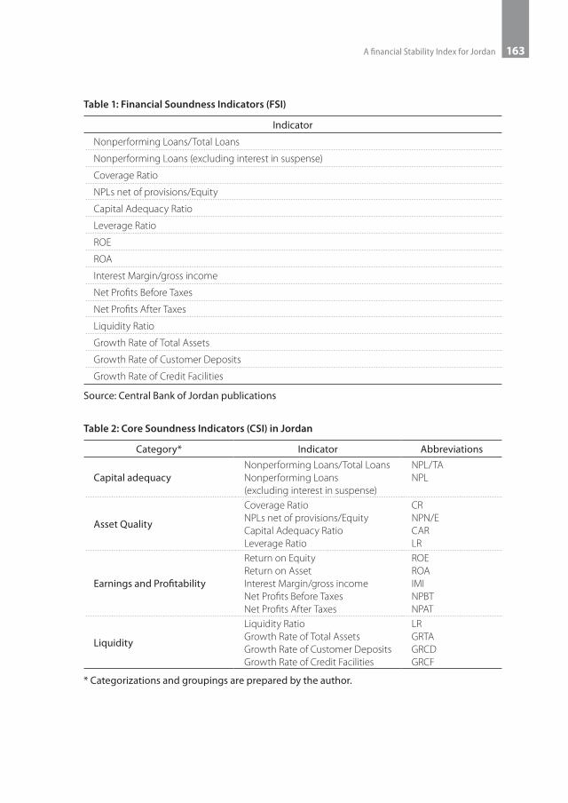
The CBJ publishes a list of indicators called financial soundness indicators. The list includes 15 different indicators related to the banking sector in Jordan. Table 1 lists those 15 indicators.

In what follows we group these 15 listed indicators into four groups: (1) Capital Adequacy, (2) Asset Quality, (3) Earnings and Profitability, and (4) Liquidity. The classification of these four groups can be found in Table (2). As can be seen, Table 2 shows that the CBJ is using a close categorization to that of the core Interna-tional Monetary Fund (IMF) financial soundness indicators for deposit takers (IMF, 2006) where the CBJ produces four categories out of five. The fifth missing category is the exposure to foreign exchange risk. It is also important to highlight that the CBJ is not reporting the regulatory capital to risk weighted assets and the regulatory Tier 1 capital to risk weighted assets. The current categorization of soundness indicators is not perfectly compatible with the CAMELS methodology for the assessment of the soundness of individual financial institutions.


Table 1: Financial Soundness Indicators (FSI)

Indicator

Nonperforming Loans/Total Loans

Nonperforming Loans (excluding interest in suspense)

Coverage Ratio

NPLs net of provisions/Equity

Capital Adequacy Ratio

Leverage Ratio

ROE

ROA

Interest Margin/gross income

Net Profits Before Taxes

Net Profits After Taxes

Liquidity Ratio

Growth Rate of Total Assets

Growth Rate of Customer Deposits

Growth Rate of Credit Facilities

Source: Central Bank of Jordan publications

Table 2: Core Soundness Indicators (CSI) in Jordan

Category* Indicator Abbreviations

Capital adequacy Nonperforming Loans/Total LoansNonperforming Loans (excluding interest in suspense)

NPL/TANPL

Asset Quality

Coverage RatioNPLs net of provisions/EquityCapital Adequacy RatioLeverage Ratio

CRNPN/ECARLR

Earnings and Profitability

Return on EquityReturn on AssetInterest Margin/gross incomeNet Profits Before TaxesNet Profits After Taxes

ROEROAIMINPBTNPAT

Liquidity

Liquidity RatioGrowth Rate of Total AssetsGrowth Rate of Customer DepositsGrowth Rate of Credit Facilities

LRGRTAGRCDGRCF

* Categorizations and groupings are prepared by the author.


The capital adequacy indicators measure the banking sector’s ability to absorb sudden losses (resilience to shocks) and their capacity to deal with potential risks, whereas the asset quality indicators are directly associated with potential risks to banks’ solvency. The profitability indicators measure the ability to absorb losses without any impact on capital, while the liquidity indicators measure bank’s re-silience to cash flow shocks.

Considering the significant role of the banking sector for monetary and finan-cial stability of the economy, the central banks and the international financial institutions, constantly monitor countries financial systems stability through the identification of the determinants and indicators of financial stability (Popovska, 2014). This can be seen in tables 1 and 2 above where all the CBJs’ FSI’s are related to the banking sector and directly measures its ability to absorb sudden losses and cash flow shock.

The indicators of financial stability established by the IMF and applied to mem-ber countries are mostly in aggregate form for the entire banking system for the purpose of supporting macroprudential analysis (macroprudential variables in-clude both macro and microprudential).

4. Data and Methodology

The aim of this paper is to develop a continuous and quantifiable measurement that can be used to determine the stress level in the Jordanian financial system. Two important steps are needed to reach this goal; First, appropriate selection of the indicators that formulate the aggregate stability index, and second, the weighting scheme followed. In what follows, data properties are discusses in sec-tion 4.1, and methodology and weighting scheme in section 4.2.

4.1. Data

Yearly data includes all of the 15 soundness indicators published by the CBJ dur-ing the period from 2003 to 2015. The 15 indicators are listed in Table 1 and categorized in Table 2. All indicators are presented in ratios except for: Nonper-forming Loans (excluding interest in suspense), Net Profits before Taxes, and Net Profits after Taxes which are in millions of Jordan Dinars (JDs). The study period includes the period of the financial crises in 2007-2008 and include data from several phases of the economic and credit cycle. The variables used to build the index are the following:


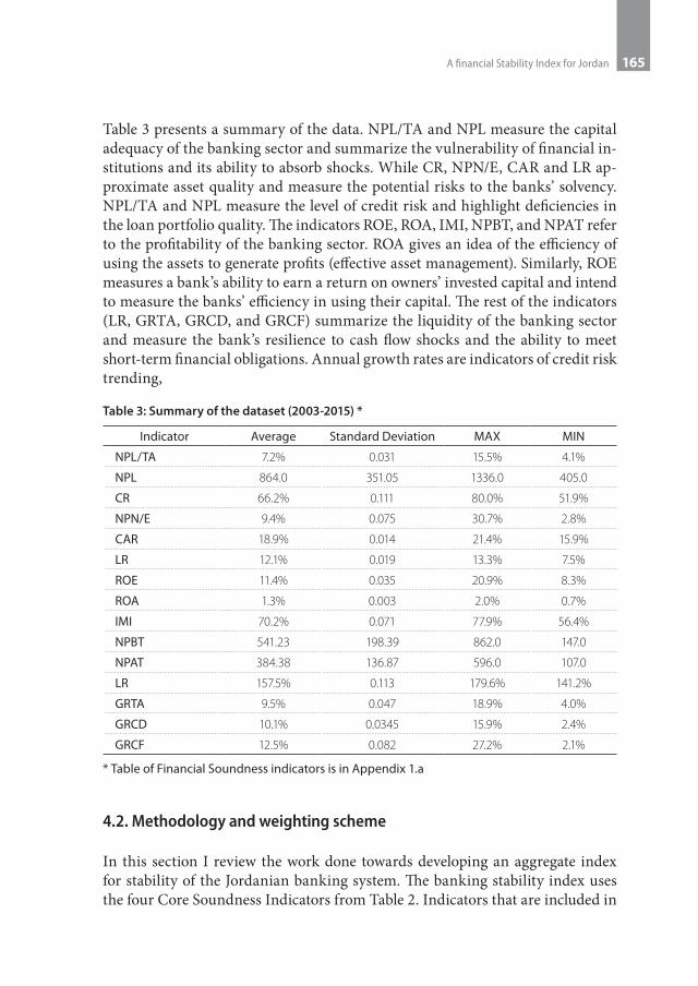
Table 3 presents a summary of the data. NPL/TA and NPL measure the capital adequacy of the banking sector and summarize the vulnerability of financial in-stitutions and its ability to absorb shocks. While CR, NPN/E, CAR and LR ap-proximate asset quality and measure the potential risks to the banks’ solvency. NPL/TA and NPL measure the level of credit risk and highlight deficiencies in the loan portfolio quality. The indicators ROE, ROA, IMI, NPBT, and NPAT refer to the profitability of the banking sector. ROA gives an idea of the efficiency of using the assets to generate profits (effective asset management). Similarly, ROE measures a bank’s ability to earn a return on owners’ invested capital and intend to measure the banks’ efficiency in using their capital. The rest of the indicators (LR, GRTA, GRCD, and GRCF) summarize the liquidity of the banking sector and measure the bank’s resilience to cash flow shocks and the ability to meet short-term financial obligations. Annual growth rates are indicators of credit risk trending,

Table 3: Summary of the dataset (2003-2015) *

Indicator Average Standard Deviation MAX MIN

NPL/TA 7.2% 0.031 15.5% 4.1%

NPL 864.0 351.05 1336.0 405.0

CR 66.2% 0.111 80.0% 51.9%

NPN/E 9.4% 0.075 30.7% 2.8%

CAR 18.9% 0.014 21.4% 15.9%

LR 12.1% 0.019 13.3% 7.5%

ROE 11.4% 0.035 20.9% 8.3%

ROA 1.3% 0.003 2.0% 0.7%

IMI 70.2% 0.071 77.9% 56.4%

NPBT 541.23 198.39 862.0 147.0

NPAT 384.38 136.87 596.0 107.0

LR 157.5% 0.113 179.6% 141.2%

GRTA 9.5% 0.047 18.9% 4.0%

GRCD 10.1% 0.0345 15.9% 2.4%

GRCF 12.5% 0.082 27.2% 2.1%

* Table of Financial Soundness indicators is in Appendix 1.a

4.2. Methodology and weighting scheme

In this section I review the work done towards developing an aggregate index for stability of the Jordanian banking system. The banking stability index uses the four Core Soundness Indicators from Table 2. Indicators that are included in


the index are those published by the central bank in accordance with the inter-national practice based on their relevance to the stability of the banking system.

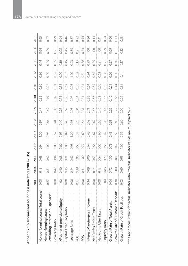
A necessary scale adjustment to the data is needed before measuring the FSI. Also, we must overcome the problems of measurement unit and accuracy levels via a suitable normalization procedure. These necessary adjustments are impor-tant in order to compare properly between indicators and to correctly aggregate them. For example, some of these indicators are in monetary values (such as Nonperforming Loans and Net Profits Before and after Taxes) and some are in ratios (such as Coverage Ratio Nonperforming Loans/Total Loans Capital Ad-equacy Ratio) and others are growth rates (such as Growth Rate of Total Assets, Growth Rate of Customer Deposits). Reciprocal value is taken for some sound-ness indicators (Nonperforming Loans and Nonperforming Loans/Total Loans) which move in opposite directions show improvement/deterioration in terms of the direction of other indicators, while the size of non-performing loans is multi-plied by (-1). Normalized and scaled financial soundness indicators are presented in Appendix 1.b.

All indicators were normalized using the max-min method. The formula used for the normalization process is as follows:

(1)

Where:

represents the normalized indicator i at time t

and is the maximum(best) and worst (Minimum) values of each indicator respectively.

The numerical values calculated using this normalization procedure are in the [0,1] range, with values close to zero indicating a weak and unstable situation, while those close to one representing a strong and stable value state.

Weighting scheme

There is no best way to determine the correct assignment of weights to each indi-cator, even though they carry a significant effect on the overall composite index.


A wide variety of methods and practices are used to weigh variables.3 For exam-ple, sometimes central banks use expert judgment and do not consider the poten-tial correlation between individual partial indicators and sometimes researchers use sophisticated non-compensatory multi-criteria approach. In this paper we use both the variance-equal weight approach and the principal components.4

The variance-equal weight assigns equal weights to each aggregated index catego-ry and in our case the assigned weights are 25% each. This methodology is used (for example) by the Central bank of the Republic of Turkey, the Bank of Albania, and the Czech National Bank, and it is also adopted by many researchers like Ko-cisova (2015), Morales and Estrada (2010)5, and Karanovic and Karanovic (2015) to some extent. Others use expert judgment without considering the potential correlations between individual partial indicators such as Gersi and Hermanek (2007, 2008). Finally, some used the sophisticated non-compensatory multi-crite-ria approach such Popovska (2014) and Morales and Estrada.

After selecting, defining, grouping, and normalizing the variables included in the aggregate index, the four sub-indices are calculated by aggregating the individual indicators in each of these sub-indices and weighting them by the number of in-dicators in each CSI as follows:

(2)

(3)

(4)

(5)

3 The Bank for International Settlement (BIS) listed five different ways to determine weighs. Firstly, common factors analysis can be performed. Secondly, a weight representing the impor-tance (size) of the market which it proxies for can be assigned to each factor. Thirdly, sample cu-mulative distribution functions can be estimated. Fourthly, the results of economic simulations with a macro-economic model can be used to determine the weights. Fifthly, the variance-equal method can be chosen.

4 Examples of other weighting schemes are: arithmetic, geometric, Zero inflated Poisson, and zero –inflated binomial negative regressions.

5 Morales and Estrada used three approaches to weight indicators namely (1) variance-equal weight, (2) principal components and count data models, (3) zero inflated Poisson and zero-inflated binomial negative regression.


For the next step, I calculate the weights for each of the four sub-indices using equal and principal components analysis approaches. The resulted weights are in Table 4:

Table 4: Weights of banking stability sub-indices under two approaches: equally weighted approach and principal components and count data model

Category Equal weights* Principal components model

Capital adequacy 0.25 0.0526

Asset Quality 0.25 0.0844

Earnings and Profitability 0.25 0.4955

Liquidity 0.25 0.3672

* BIS reports that variance equal weights are the one most commonly used in the literature and consists of normalizing each variable and then assigning equal weights.

For the last step, we calculate the FSI (i.e. the BSI) as a weighted average (using two weights approaches) of the four Core Soundness Indicators (CSI) namely Capital Adequacy (CA), Asset Quality (AQ) , Earnings and Profitability (EP), and Liquidity ( L) .

Equation 6 presents ωi as the weight of each of the four categories used in the composition of the index and the resulted FSI is a weighted average of these four categories. The sum of the weights is one.

(6)

The two equations use for calculating the FSI are as follows:

(1) Equal weights:

(2) Principal components model weights:

5. Results

Results for aggregating the FSI are under two scenarios: (i) equal weights of the constituent Sub-indexes and (ii) Principal component analysis.


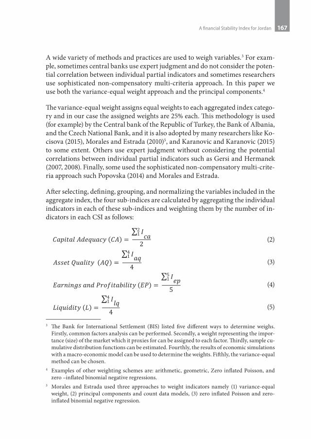
Scenario (i): The aggregate FSI for Jordan is constructed using annual data for the 2003-2015 periods. Normalized and weighted values of the composite sub-indices along with their totals can be seen in Table 5. According to the methodol-ogy described previously, the increase in the index means improved bank stabil-ity, while the decrease denotes stability worsening. FSI and sub-indices graph is figure 1.

Table 5: Financial Stability Index (FSI) and the four sub-indices

Year Asset Quality Capital Adequacy

Earnings and Profitability Liquidity FSI

2003 0.33 0.25 0.09 0.34 0.25

2004 0.50 0.35 0.21 0.81 0.47

2005 0.70 0.46 0.61 0.87 0.66

2006 0.97 0.75 0.61 0.75 0.77

2007 0.97 0.63 0.55 0.50 0.66

2008 0.91 0.47 0.54 0.48 0.60

2009 0.48 0.48 0.40 0.36 0.43

2010 0.25 0.53 0.45 0.45 0.42

2011 0.16 0.49 0.41 0.33 0.35

2012 0.18 0.60 0.51 0.13 0.36

2013 0.25 0.60 0.63 0.33 0.45

2014 0.46 0.57 0.75 0.25 0.51

2015 0.46 0.59 0.49 0.14 0.42

Figure 1: Jordan Financial stability Index (FSI) AND Constituent Sub-indexes (2003-2015)


The FSI average weighted value for the entire period is 0.49, it reached its all-time high in 2006 and an all-time low in 2003 with the values of 0.77 and 0.25, respectively.

The FSI spikes in 2006 with value for the aggregate index at 0.77, explaining a pe-riod of high economic growth. The index declines sharply from 2007 to 2011 with values at 0.66, 0.34, 0.42, and 0.35, respectively and then stabilized between 2011 and 2012 to rise up again in 2013 and 2015 with values of 0.45 and 0.51, respec-tively. The FSI sharp decline after 2006 reflects the negative effect of the financial crises spillover on banks and the slowing down of the growth rate GDP. The FSI declines in value in 2015 at 0.42, explaining declined liquidity and earnings and profits as can be seen in the downtrend trend of Liquidity index (from 0.25 to 0.14) and Earnings and Profitability index (from 0.75 to 0.45).

Figure 1 also shows that capital adequacy indicators decline sharply from 2008 to 2011 with values at 0.91, 0.48, 0.25, and 0.16, respectively and thus reflect the weakening banking sector’s ability to absorb sudden losses (weak resilience to shocks) and its capacity to deal with potential risks during this period. However, the Capital Adequacy indicator shows prominent improvement after 2012 until 2015.


The liquidity indicator which also measure bank’s resilience to cash flow shocks and their success in cash flow management shows declining trend from 2005 and onward and reach a global minimum of 0.14 in 2015.

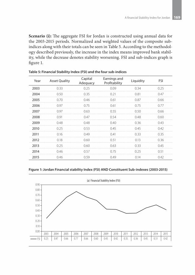
Figure 2 plots the FSI along with the GDP growth rate (at current mar-ket price) for the period from 2003 to 2015 and shows the strong correlation between FSI movement and the GDP growth rate; the correlation coefficient is 0.63.

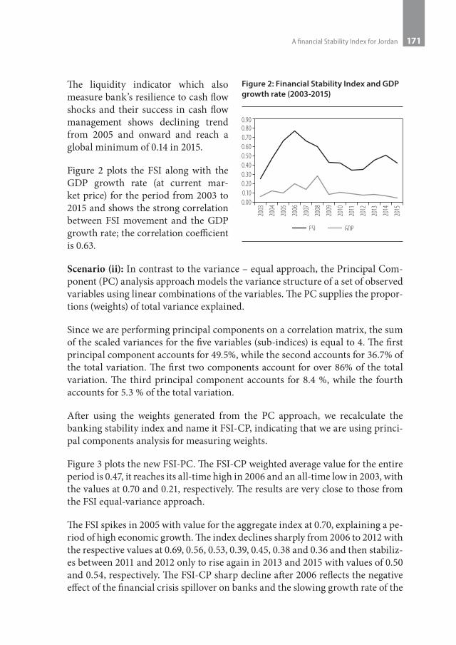
Scenario (ii): In contrast to the variance – equal approach, the Principal Com-ponent (PC) analysis approach models the variance structure of a set of observed variables using linear combinations of the variables. The PC supplies the propor-tions (weights) of total variance explained.

Since we are performing principal components on a correlation matrix, the sum of the scaled variances for the five variables (sub-indices) is equal to 4. The first principal component accounts for 49.5%, while the second accounts for 36.7% of the total variation. The first two components account for over 86% of the total variation. The third principal component accounts for 8.4 %, while the fourth accounts for 5.3 % of the total variation.

After using the weights generated from the PC approach, we recalculate the banking stability index and name it FSI-CP, indicating that we are using princi-pal components analysis for measuring weights.

Figure 3 plots the new FSI-PC. The FSI-CP weighted average value for the entire period is 0.47, it reaches its all-time high in 2006 and an all-time low in 2003, with the values at 0.70 and 0.21, respectively. The results are very close to those from the FSI equal-variance approach.

The FSI spikes in 2005 with value for the aggregate index at 0.70, explaining a pe-riod of high economic growth. The index declines sharply from 2006 to 2012 with the respective values at 0.69, 0.56, 0.53, 0.39, 0.45, 0.38 and 0.36 and then stabiliz-es between 2011 and 2012 only to rise again in 2013 and 2015 with values of 0.50 and 0.54, respectively. The FSI-CP sharp decline after 2006 reflects the negative effect of the financial crisis spillover on banks and the slowing growth rate of the

Figure 2: Financial Stability Index and GDP growth rate (2003-2015)


GDP. The FSI decline in value in 2015 at 0.37, explaining declined liquidity and earnings and profits as can be seen in the downtrend trend of the Liquidity index (from 0.25 to 0.14) and the Earnings and Profitability index (from 0.75 to 0.45).

Overall, the results of FSI and FSI-CP are very close and reflect the general sound-ness of the financial system and the economy. This is consistent with of Van den End (2006) where he showed a small discrepancy between equal weighting and weighting by scaling of weights and non-linear effects in his effort to build a fi-nancial conditions index for stability.

Figure 3: Jordan Banking stability Index using Principal Components Analysis (FSI-PC) and Constituent Sub-indexes (2003-2015)


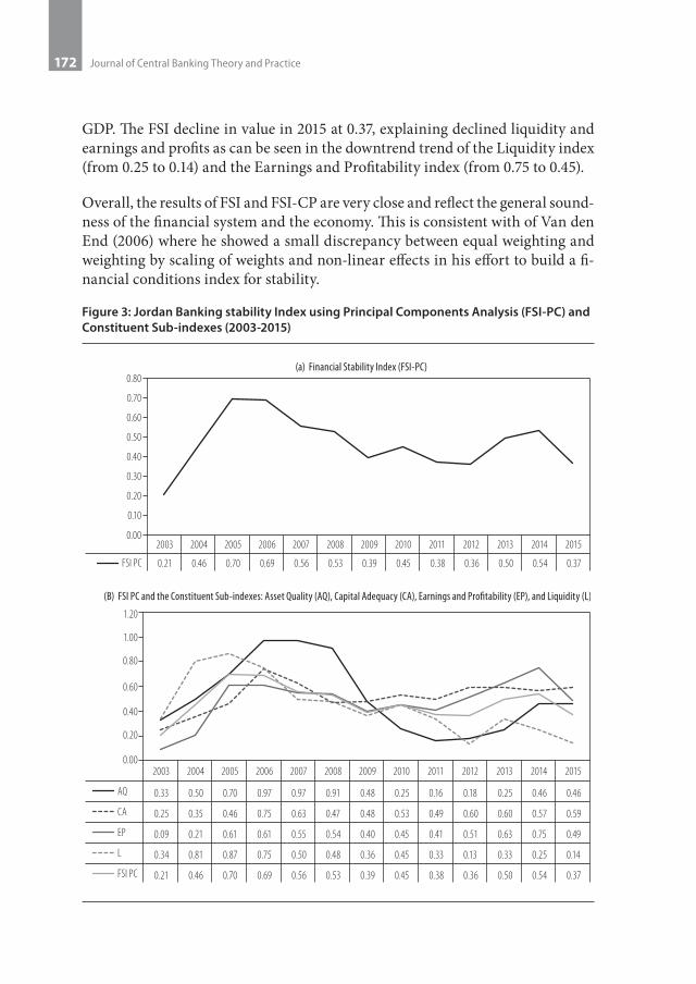
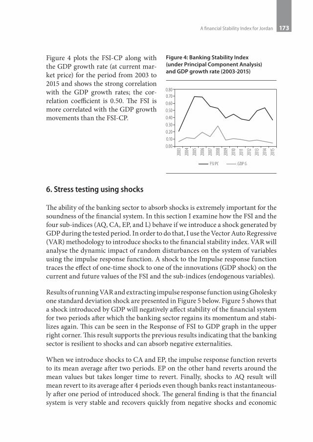
Figure 4 plots the FSI-CP along with the GDP growth rate (at current mar-ket price) for the period from 2003 to 2015 and shows the strong correlation with the GDP growth rates; the cor-relation coefficient is 0.50. The FSI is more correlated with the GDP growth movements than the FSI-CP.

6. Stress testing using shocks

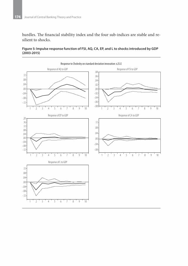
The ability of the banking sector to absorb shocks is extremely important for the soundness of the financial system. In this section I examine how the FSI and the four sub-indices (AQ, CA, EP, and L) behave if we introduce a shock generated by GDP during the tested period. In order to do that, I use the Vector Auto Regressive (VAR) methodology to introduce shocks to the financial stability index. VAR will analyse the dynamic impact of random disturbances on the system of variables using the impulse response function. A shock to the Impulse response function traces the effect of one-time shock to one of the innovations (GDP shock) on the current and future values of the FSI and the sub-indices (endogenous variables).

Results of running VAR and extracting impulse response function using Gholesky one standard deviation shock are presented in Figure 5 below. Figure 5 shows that a shock introduced by GDP will negatively affect stability of the financial system for two periods after which the banking sector regains its momentum and stabi-lizes again. This can be seen in the Response of FSI to GDP graph in the upper right corner. This result supports the previous results indicating that the banking sector is resilient to shocks and can absorb negative externalities.

When we introduce shocks to CA and EP, the impulse response function reverts to its mean average after two periods. EP on the other hand reverts around the mean values but takes longer time to revert. Finally, shocks to AQ result will mean revert to its average after 4 periods even though banks react instantaneous-ly after one period of introduced shock. The general finding is that the financial system is very stable and recovers quickly from negative shocks and economic

Figure 4: Banking Stability Index (under Principal Component Analysis) and GDP growth rate (2003-2015)


hurdles. The financial stability index and the four sub-indices are stable and re-silient to shocks.

Figure 5: Impulse response function of FSI, AQ, CA, EP, and L to shocks introduced by GDP (2003-2015)


7. Conclusion

This paper develops a quantitative measure of financial stability that can be used to determine the stress level of the Jordanian financial system. The composite measure can be used to sense future turbulences in the financial system even in the absence of negative shocks. This developed Financial Stability Index (FSI) is a trustful indicator that can monitor the financial system and give a clear overview of the system vulnerabilities.

The approaches used were the variance-equal approach and the principal compo-nents method. I constructed an index that presented a similar behaviour under the two different methodologies and which, in general, gave a high weight to the Earning and Profitability (EP) (0.496) and Liquidity (L) (0.367) sub-indices.

These quantitative aggregate measures of financial system stability are intuitively attractive as they could enable policy makers to better monitor the banking sec-tor’s resilience to shocks and their capacity to deal with potential risks and fur-ther help in anticipating the sources and causes of financial stress to the system.

The discussion on the FSI pros and cons, however, suggests that the developed index does not consider a number of potential risks related to foreign exchange exposure or off-balance sheet items. Nonetheless, it is a good foundation for con-structing more comprehensive indicators, such as using the CAMELS approach for the classification of indicators that signal certain uncertainties or indices of financial stress that are used for crisis prediction.

The index of financial stability of the banking sector in Jordan shows that the banking system has been consciously resilient to external shocks and to negative local economic conditions. This is also supported by the results of stress testing using shocks introduced through VAR.


References:

1. Bank of Albania, 2010, Financial Stability Report, Tirana: Bank of Albania.2. Central Bank of Jordan, 2015, Financial Stability Report.3. Central Bank of the Republic of Turkey, 2008, Financial Stability Report,

Ankara: Central Bank of the Republic of Turkey.4. Dumičić, M., 2016, Financial Stability Indicators – The Case of Croatia,

Journal of Central Banking Theory and Practice, 5, 1, 113-140.5. Morales, M. A. and Estrada, D., 2010, A financial stability index for

Colombia, Ann Finance, 6, 555-581.6. Gersi, A. and Hermanek, J., 2008, Indicators of financial system stability:

towards an aggregate financial stability indicator, Prague Economic Papers, 3, 127-142.

7. Gersi, A. and Hermanek, J., 2007, Financial stability indicators: advantages and disadvantages of their use in the assessment of financial system stability, CNB Financial Stability Report 2006,2007, 69-79, Czech National Bank.

8. International Monetary Fund, 2006, Compilation Guide, retrieved from: https://www.imf.org/external/pubs/ft/fsi/guide/2006/pdf/fsiFT.pdf

9. Karanovic, G. and Karanovic, B., 2015. Developing an aggregate index for measuring financial stability in the Balkans, Procedia Economics and Finance 33, 3-17.

10. Kocisova, K., 2015, Banking stability index: a cross-country study, 15th international conference of finance and banking proceedings, page 197.

11. Kondratovs, K., 2012, Modelling financial stability index for Latvian financial system, Regional Formation and Development Studies, 3,8, 118-129.

12. Popovska, J., 2014, Modeling financial stability: the case of the banking sector in Macedonia, Journal of applied economics and business, 2, 1, 68-91.

13. Petrovska, M. and Mucheva Mihajlovska, E., 2013, Measures of financial stability in Macedonia, Journal of Central Banking Theory and Practice, 3, 85-110.

14. Ginevicius, R. and Podviezko, A., 2013, The evaluation of financial stability and soundness of Lithuanian banks, Economic Research, 26,2,191-208.

15. Tintchev, K. I., 2014, Interconnectedness, vulnerabilities, and crisis spillovers: implications for the new financial stability framework, unpublished dissertation, The Faculty of The Columbian College of Arts and Sciences, George Washington University.

16. Van Den End, J. W., 2006, Indicators and boundaries of stability. DNB Working Paper, No. 097/March 2006.


App

endi

x 1.

a: F

inan

cial

Sou

ndne

ss In

dica

tors

(Jor

dan

Bran

ches

)

Indi

cato

r20

0320

0420

0520

0620

0720

0820

0920

1020

1120

1220

1320

1420

15

Non

perf

orm

ing

Loan

s/To

tal L

oans

0.15

50.

103

0.06

60.

043

0.04

10.

042

0.06

70.

082

0.08

50.

077

0.07

0.05

60.

049

Non

perf

orm

ing

Loan

s (e

xclu

ding

inte

rest

in s

uspe

nse)

*71

658

148

140

545

355

087

711

5913

1513

3612

8510

6410

10

Cove

rage

Rat

io0.

519

0.63

80.

784

0.8

0.67

80.

634

0.52

0.52

40.

523

0.69

40.

770.

776

0.74

7

NPL

s ne

t of p

rovi

sion

s/Eq

uity

0.30

70.

139

0.05

10.

028

0.04

30.

057

0.10

60.

126

0.13

40.

083

0.05

60.

043

0.04

5

Capi

tal A

dequ

acy

Ratio

0.15

90.

178

0.17

60.

214

0.20

80.

184

0.19

60.

203

0.19

30.

190.

184

0.18

40.

191

Leve

rage

Rat

io0.

075

0.08

90.

105

0.13

20.

133

0.12

90.

130.

131

0.13

10.

133

0.12

90.

125

0.12

7

ROE

0.09

90.

131

0.20

90.

150.

126

0.11

50.

088

0.08

80.

083

0.08

60.

099

0.11

0.10

3

ROA

0.00

70.

011

0.02

0.01

70.

016

0.01

40.

011

0.01

10.

011

0.01

10.

012

0.01

40.

013

Inte

rest

Mar

gin/

gros

s in

com

e0.

637

0.58

30.

564

0.70

20.

667

0.71

30.

716

0.74

30.

701

0.76

60.

776

0.77

90.

774

Net

Pro

fits

Befo

re T

axes

*14

724

050

252

356

956

446

052

351

758

871

982

286

2

Net

Pro

fits

Aft

er T

axes

*10

717

136

937

540

040

033

336

638

241

450

259

658

2

Liqu

idity

Rat

io1.

796

1.73

1.68

1.61

41.

575

1.41

21.

591

1.61

41.

529

1.43

51.

491

1.52

21.

49

Gro

wth

Rat

e of

Tot

al A

sset

s0.

040.

145

0.18

90.

157

0.10

90.

114

0.07

40.

096

0.07

90.

043

0.09

10.

049

0.05

1

Gro

wth

Rat

e of

Cus

tom

er D

epos

its0.

064

0.15

90.

134

0.11

40.

096

0.13

20.

121

0.10

90.

083

0.02

40.

105

0.09

30.

077

Gro

wth

Rat

e of

Cre

dit F

acili

ties

0.02

70.

193

0.25

90.

272

0.16

10.

172

0.02

10.

086

0.09

80.

125

0.06

30.

052

0.09

6

*in

mill

ions

of J

orda

n D

inar


App

endi

x 1.

b: N

orm

aliz

ed s

ound

ness

indi

cato

rs (2

003-

2015

)

2003

2004

2005

2006

2007

2008

2009

2010

2011

2012

2013

2014

2015

Non

perf

orm

ing

Loan

s/To

tal L

oans

*0.

000.

180.

480.

941.

000.

970.

470.

320.

300.

360.

440.

640.

65

Non

perf

orm

ing

Loan

s (e

xclu

ding

inte

rest

in s

uspe

nse)

**0.

670.

810.

921.

000.

950.

840.

490.

190.

020.

000.

050.

290.

27

Cove

rage

Rat

io0.

000.

420.

941.

000.

570.

410.

000.

020.

010.

620.

890.

910.

99

NPL

s ne

t of p

rovi

sion

s/Eq

uity

1.00

0.40

0.08

0.00

0.05

0.10

0.28

0.35

0.38

0.20

0.10

0.05

0.04

Capi

tal A

dequ

acy

Ratio

0.00

0.35

0.31

1.00

0.89

0.45

0.67

0.80

0.62

0.57

0.45

0.45

0.46

Leve

rage

Rat

io0.

000.

240.

520.

981.

000.

930.

950.

970.

961.

000.

930.

850.

87

ROE

0.13

0.38

1.00

0.53

0.34

0.25

0.04

0.04

0.00

0.02

0.13

0.21

0.22

ROA

0.00

0.31

1.00

0.77

0.69

0.54

0.31

0.31

0.31

0.31

0.38

0.54

0.54

Inte

rest

Mar

gin/

gros

s in

com

e0.

340.

090.

000.

640.

480.

690.

710.

830.

640.

940.

991.

000.

84

Net

Pro

fits

Befo

re T

axes

0.00

0.14

0.53

0.56

0.62

0.62

0.46

0.56

0.55

0.65

0.85

1.00

0.44

Net

Pro

fits

Aft

er T

axes

0.00

0.13

0.54

0.55

0.60

0.60

0.46

0.53

0.56

0.63

0.81

1.00

0.41

Liqu

idity

Rat

io1.

000.

830.

700.

530.

420.

000.

470.

530.

300.

060.

210.

290.

24

Gro

wth

Rat

e of

Tot

al A

sset

s0.

040.

721.

000.

790.

480.

510.

260.

400.

290.

060.

370.

090.

00

Gro

wth

Rat

e of

Cus

tom

er D

epos

its0.

301.

000.

810.

670.

530.

800.

720.

630.

440.

000.

600.

510.

19

Gro

wth

Rat

e of

Cre

dit F

acili

ties

0.02

0.69

0.95

1.00

0.56

0.60

0.00

0.26

0.31

0.41

0.17

0.12

0.13

* th

e re

cipr

ocal

is ta

ken

for a

ctua

l ind

icat

or ra

tio. *

*act

ual i

ndic

ator

val

ues

are

mul

tiplie

d by

-1.

A financial Stability Index for Jordan [email protected]

Documents

Transcript of A financial Stability Index for Jordan [email protected]