A Few Notes on Sets of Probability Distributions

Fabio G. CozmanEscola Politecnica, Universidade de Sao Paulo

fgcozman@usp.br — http://www.poli.usp.br/p/fabio.cozman

June 28, 2008

A person looks at the sky, and tries to assess what she expectsabout the weather in thenear future; another person weighs the costs of a financial application against its expected gain.Such expectations can sometimes be translated into a singlenumber: for instance, the expectedreturn on the financial application may be exactly 100 monetary units. More often, one has lessdeterminate assessments about expectations, such as “I expect a return between 30% and 40%on this investiment.” Or perhaps, “I’d rather bet that it will rain tomorrow than that I get headsin the next toss of this coin.” In general, assessments specify a set of probability distributionsthat represent the uncertainty about a particular situation. This initial chapter introduces someconcepts and tools that are useful in dealing with such sets.

1 Possibility space, states, events

The first element of this investigation is theset of possible states of the world. Each state is acomplete description of all aspects of the world that are of interest; states are mutually exclu-sive. This set of states, denoted byΩ, is called thepossibility space. (Often Ω is called thesample space, and states are calledsamples, elements, outcomes, realizations. Discussion onterminology can be found in Section 15.)

The following examples present possibility spaces that arebinary, finite, countably and un-countably infinite.

Example 1.1. We are interested in the weather forecast for next week. Among the manyphenomena that interfere with such a forecast, we focus on just two possibilities: the weathermay beSunnyor Rainy. The possibility space isΩ = Sunny, Rainy.

1

Example 1.2.Two coins are tossed; each coin can be heads (H) or tail (T ). The possibilityspace isΩ = HH,HT, TH, TT.

Example 1.3.A coin is to be tossedn times, and we are interested in the number of headsthat we will see in the sequence of tosses. If we take that the sequence may go on forever,the number of heads belongs toΩ = 0, 1, 2, . . . . That is, the possibility space is the set ofnon-negative integers.

Example 1.4. Suppose we consider infinite sequences of zeros and ones thatare perhapsproduced by tossing coins, and suppose we understand each sequenceω as the real num-ber 0.ω expressed in the binary numeral system. For instance, the sequence1, 0, 0, . . . is0.100 . . . , that is, the real number1/2. Now the possibility space of all such real numbers isthe real intervalΩ = [0, 1].

An eventis a subset ofΩ. The interpretation is that an eventA obtains when a stateω inA obtains. There is no fuzziness in our states and events: an event either obtains or does notobtain. For example, the sentence “Mary is young” does not specify an event unless we have arule that decides exactly when the predicade “is young” is true. Suppose “young” means “lessthan 18 years old.” Then the sentences “Mary is young” and “Mary is less than 18 years old” areequivalent and both define an event.

Example 1.5.Two coins are tossed. Consider three events. EventA = HH is the eventthat both tosses produce heads. EventB = HH,TT is the event that both tosses produceidentical outcomes. EventC = HH,TH is the event that the second toss yields heads.

The superscriptc denotes complement with respect toΩ; for example,Ac is the event con-taining all states not inA. The intersectionof eventsA andB is denoted byA ∩ B; that is, theevent containing states both inA and inB. Theunionof eventsA andB is denoted byA ∪ B;that is, the event containing states inA or B or both.

When we are dealing with an eventA and this event obtains, we often say that we have asuccess; if insteadAc obtains, we say that we have afailure.

2 Variables and indicator functions

Once we have a possibility space, we can imagine a function from Ω to the real numbers. Anysuch functionX : Ω → < is called arandom variable. The shorter termvariable is oftenemployed when referring to random variables. The set of all possible values of variableX isdenoted byΩX .

A random variable is always denoted by capital lettersX, Y , Z, etc. A particular value of a

2

variable is not capitalized. For example,x denotes a value ofX, andX = x denotes the eventω ∈ Ω : X(ω) = x.

If X is a variable, then any functionf : < → < defines another random variablef(X).Similarly, a function of several random variables is a random variable.

Example 2.1. The age in months of a personω selected from a populationΩ is a variableX. The same population can be used to define a different variable Y whereY (ω) is theweight (rounded to the next kilogram) of a personω selected fromΩ. ThenZ = X + Ydefines yet another random variable.

Example 2.2. Supposen coins are tossed. The possibility space contains2n possible se-quences of heads and tails. Now define variableX(ω) as the number of coins that land headsin ω. The value ofX ranges from0 to n. This variable can be used to define interestingevents, such asω : X(ω) ≤ n/2 andω : 5 ≤ X(ω) ≤ 10 (if n < 5 then the secondevent is the empty set).

Every event can be associated with a random variableIA, called itsindicator function, suchthatIA(ω) = 1 if ω ∈ A andIA(ω) = 0 otherwise. Any random variable can be expressed as alinear, perhaps infinite, combination of indicator functions:

X =∑

ω∈Ω

X(ω)Iω. (1)

This expression holds because for eachω′ ∈ Ω such thatω 6= ω′, Iω(ω′) is zero. So, for everyω′ ∈ Ω, both sides of Expression (1) refer toX(ω′).

Indicator functions do deserve some attention, as they let Boolean operations be easily ex-pressed as pointwise algebraic operations. For example, the intersection of eventsA andB hasindicator function

IA∩B = min(IA, IB) = IAIB.

As another example,IAc = 1 − IA. As a third example, consider unions of eventsAini=1. We

haveI∪ni=1

Ai= maxi IAi

, and if all events are disjoint, then

I∪ni=1

Ai=

n∑

i=1

IAi.

BecauseA ∪ B = (A ∩ Bc) ∪ (Ac ∩ B) ∪ (A ∩ B) and the latter three events are disjoint,

IA∪B = IA(1 − IB) + (1 − IA)IB + IAIB = IA + IB − IAIB.

Indicator functions are very useful devices, but sometimesthey lead to heavy notation withtoo many subscripts. It is better to usede Finetti’s convention: use the same symbol for an

3

event and its indicator function. For example, instead of writing A ∩ B = IAIB, we now writeA ∩ B = AB. Likewise,

A ∪ B = A + B − AB,

and if the eventsAini=1 are all disjoint, then

∪ni=1Ai =

n∑

i=1

Ai.

As another example, consider an expression that mixes set and algebraic notation:

(A ∩ Bc) ∪ (Ac ∩ B) = A(1 − B) + (1 − A)B = (A − B)2.

While such expressions may seem perplexing at first, they do simplify matters. Consider the fol-lowing important result on general unions, and note how muchde Finetti’s convention simplifiesthe notation.

Theorem 2.1.Given eventsAini=1, then

∪ni=1Ai =

n∑

j=1

(−1)j+1Aj,n, (2)

whereAj,n =∑

1≤i1<i2<···<ij≤n Ai1 ∩ Ai2 ∩ · · · ∩ Aij .

Proof. The casen = 2 has been proven (that is,A ∪ B = A + B − AB). Now consider an inductionargument: suppose the theorem holds forn− 1 eventsA1 to An−1. Note that∪n

i=1Ai = An + ∪n−1i=1 Ai −

An ∩(

∪n−1i=1 Ai

)

, using the fact thatA∪B = A + B −AB. As An ∩(

∪n−1i=1 Ai

)

= ∪n−1i=1 Ai ∩An, we can

use the induction hypothesis twice to obtain:

∪ni=1Ai = An + (3)

∑

1≤i≤n−1

Ai −∑

1≤i1<i2≤n−1

Ai1 ∩ Ai2 +∑

1≤i1<i2<i3≤n−1

Ai1 ∩ Ai2 ∩ Ai3 − . . .

−

∑

1≤i≤n−1

Ai ∩ An −∑

1≤i1<i2≤n−1

Ai1 ∩ Ai2 ∩ An + . . .

.

By grouping terms we obtain Expression (2).

3 Expectations

Suppose one is willing to “buy” a random variableX for any amountα that is strictly smallerthan some numberE[X]. The result of payingα and gettingX is

X − α.

4

Now suppose the person is willing to “sell”X for any amountβ that is strictly larger than somenumberE[X]. The result of sellingX for β is

β − X.

We should expect thatE[X] ≥ E[X], for otherwise we might put our subject in a trulyembarrassing situation, as follows. Suppose

E[X] − E[X] = −δ for someδ > 0;

then by definition ofE[X] andE[X], the person must be willing to buyX for E[X] − δ/3 andthen to sellX for E[X] + δ/3. The net result of such transactions is

(X − (E[X] − δ/3)) + ((E[X] + δ/3) − X) = E[X] − E[X] + 2δ/3

= −δ/3 < 0.

So, if E[X] ≤ E[X], then the person stands to lose by engaging in two transactions that she, bydefinition, was willing to accept!

Suppose that for some random variableX we haveE[X] = E[X]. We then denote byE[X]the valueE[X] = E[X], and refer to it as theexpectationof X. The expectation of a randomvariableX can be interpreted as a “fair price” forX: our subject is willing to buyX for less thanE[X], and is willing to sellX for more thanE[X].

If we find ourselves in the excepcional circumstance that an unique expectationE[X] is givenfor every variableX, we can treatE[·] as a single entity, called anexpectation functional. Weassume that any expectation functional should satisfy:

Definition 3.1 (Axioms for expectation functionals).

EU1 For constantsα andβ, if α ≤ X ≤ β, thenα ≤ E[X] ≤ β.

EU2 E[X + Y ] = E[X] + E[Y ].

The first axiom is quite reasonable: the fair price forX cannot be smaller than the smallestvalue ofX, and likewise for the largest value ofX. The second axiom takes the fair price ofX + Y as simply the fair price ofX plus the fair price ofY .

Some consequences of the axioms are obvious: for instance, if α is a real number,E[α] = αby EU1. And then, for anyX,

E[X + (−X)] = E[X] + E[−X] = 0

and consequently:E[X] = −E[−X] . (4)

The axioms have a number of consequences that are worth stating explicitly (note thatX ≥ YmeansX(ω) ≥ Y (ω) for anyω ∈ Ω):

5

Theorem 3.1. An expectation functional satisfies, for any real numberα and variablesX andY :

1. X ≥ Y ⇒ E[X] ≥ E[Y ].

2. E[αX] = αX.

Proof. If X ≥ Y , then

X − Y ≥ 0 ⇒ E[X − Y ] ≥ 0 ⇒ E[X] + E[−Y ] ≥ 0 ⇒ E[X] ≥ −E[−Y ] ⇒ E[X] ≥ E[Y ] .

For the second statement, start by noting that, for any integern > 0, E[nX] = E[∑n

i=1 X] =∑n

i=1 E[X]using finite induction on EU2. For two integersn > 0 andm > 0, E[Y ] = (n/n)E[Y ] = (1/n)E[nY ]andE[Y ] = (m/m)E[Y ] = (1/m)E[mY ]; thus (1/n)E[nY ] = (1/m)E[mY ]. TakeX = Y/m toobtainE[nX/m] = (n/m)E[X]. So the second statement holds ifα is a positive rational.

If α is not rational, recall that the rationals are dense in the reals (that is, there is always a rationalbetween two distinct reals). AssumeX ≥ 0. If E[X] = 0, thenαE[X] = E[αX] = 0 and the desiredresult obtains). Assume thenE[X] > 0, and produce a contradiction by assumingαE[X] < E[αX].Find a rationalr such thatα < r < E[αX] /E[X]. Then: (a)α < r ⇒ αX < rX ⇒ E[αX] < E[rX];(b) r < E[αX] /E[X] ⇒ rE[X] < E[αX] ⇒ E[αX] > E[rX]. So we get a contradiction. A similarcontradiction obtains if we assume thatαE[X] > E[αX]. ThusαE[X] = E[αX] if X ≥ 0.

If X is not always nonnegative, then writeX asY −Z, whereY = max(X, 0) andZ = max(−X, 0),and use the fact thatE[−Z] = −E[Z] to produce the result as follows:E[αX] = E[αY − αZ] =E[αY ] − E[αZ] = αE[Y ] − αE[Z] = αE[X].

Thus, expectation functionals arelinear becauseE[αX + βY ] = αE[X] + βE[Y ], and aremonotonebecauseX ≥ Y impliesE[X] ≥ E[Y ].

Example 3.1. SupposeΩ = ω1, ω2, ω3 and take the four variables in Table 1. Supposewe know that a person has bounds on her fair prices such thatE[Xi] ∈ [µi, νi], whereµi andνi are also indicated in Table 1.

Take an additional variableX5 such thatX5(ω1) = 3, X5(ω2) = −1, X5(ω3) = 2. AxiomEU1 requires thatE[X5] ∈ [−1, 3]. As X5 = X1 + X2 + 2X3, axioms EU1-EU2 imply

E[X5] = E[X1] + E[X2] + 2E[X3] .

There is no unique fair price forX5 given the assessments in Table 1. All we can say is thatfair prices forX5 must belong to an interval[µ5, ν5]. Certainly

µ5 ≥ µ1 + µ2 + 2µ3 = 1/3,

andν5 ≤ ν1 + ν2 + 2ν3 = 10/3.

Actually, the best bounds onE[X5] are[11/18, 11/6]; an easy method to obtain such boundsis discussed in Example 6.2.

6

Xi Xi(ω1) Xi(ω2) Xi(ω3)X1 1 0 0X2 2 −1 0X3 0 0 1X4 −1 0 1

µi νi

0 2/30 2

1/6 1/3−1 0

Table 1: Variables and bounds on their prices (Example 3.1).

It remains to examine the relationship between fair pricesE[X], the “maximum buying price”E[X], and the “minimum selling price”E[X]. Consider the following rationale:

• If one holds a set of expectations forX, then this person must be willing to buyX for anyamount smaller thaninf E[X].

• Likewise, the person must be willing to sellX for any amount larger thansup E[X].

For instance, in Example 3.1 we should take eachµi as the lower expectationE[Xi], and likewiseνi should be the upper expectationE[Xi]. We are thus led to the definition:

Definition 3.2. The lower expectation and theupperexpectation of variableX are respectively

E[X] = inf E[X] and E[X] = sup E[X] .

For any variable,E[X] = −E[−X] because

E[X] = − sup E[−X] = −E[−X] . (5)

If α ≤ X ≤ β, then clearly

α ≤ E[X] ≤ β, α ≤ E[X] ≤ β.

Also, for α > 0 (note:α is nonnegative!),

E[αX] = αE[X] , E[αX] = αE[X] .

Moreover, for any two variablesX andY ,

E[X + Y ] = inf E[X + Y ] ≥ inf E[X] + inf E[Y ] = E[X] + E[Y ]

andE[X + Y ] = sup E[X + Y ] ≤ sup E[X] + sup E[Y ] = E[X] + E[Y ]

The discussion so far has implicitly assumed thatE[X] andE[X] are finite; otherwise, wemay run into difficulties wheneverE[X] = E[X] = ∞. In this chapter we adopt the followingassumption, which is enough to avoid problems given axioms EU1-EU2 and Definition 3.2:

Assumption 3.1.Every random variable is bounded.

7

4 Some consequences of the axioms

The assessment of expectations for some variables constrains the values of other assessmentsthrough axioms EU1-EU2. Here we examine a few such constraints.

4.1 Simple variables and their expectations

A random variable issimpleif it may assume only a finite number of different values. A simplevariableX can always be written as follows:

X =n∑

i=1

αiAi,

for a set of numbersαi and indicator functionsAi. Axioms EU1-EU2 imply:

E[X] = E

[

n∑

i=1

αiAi

]

=

n∑

i=1

E[αiAi] =

n∑

i=1

αiE[Ai] .

Obviously, if the possibility space is finite then any variable is simple. In this case we canuse Expression (1) and write:

E[X] = E

[

∑

ω∈Ω

X(ω)Iω

]

=∑

ω∈Ω

X(ω)E[Iω] . (6)

In words: if the possibility space is finite, every expectation functional is defined uniquely by theexpectationsE[Iw] for eachω ∈ Ω.

Example 4.1.A six-sided die is rolled. The possibility space isΩ = 1, 2, 3, 4, 5, 6. Vari-ableX maps1, 3, 5 to zero and2, 4, 6 to one (X is the indicator function of “an evennumber obtains”). VariableY maps a face withi pips to2i. Suppose the expectations forE[ωi] have been assessed, fori = 1 . . . 6. Note that we useE[wi] instead of the more cumber-some notationE[Iwi

]. We haveE[X] = E[ω2]+E[ω4]+E[ω6] andE[Y ] =∑6

i=1 2iE[ωi].If W = XY 2, thenE[W ] = 16E[ω2] + 64E[ω4] + 144E[ω6].

We might try to use simple variables to help in computing the expectation for variables ininfinite possibility spaces. For a variableX, consider the set of all simple variablesY such thatX ≥ Y . For all thoseY , we haveE[X] ≥ Y . It is reasonable to expect that the supremum ofE[Y ] for all suchY will approximateE[X] rather well:

E[X] ≈ sup (E[Y ] : Y is simple andX ≥ Y ) .

This strategy is indeed successful, in the sense thatE[X] is equal tosup E[Y ], in many situations.

8

4.2 Inequalities: Jensen, Holder, Cauchy-Scharwz

Inequalities are quite important because they allow us to bound quantities, sometimes quite ac-curately, even when we have few values of expectations at hand. Some inequalities are so usefulthat they receive special names.

Theorem 4.1(Jensen inequality). If f(X) is a convex function,f(E[X]) ≤ E[f(X)].

Proof. If f(X) is convex, there is a line through the point(E[X] , f(E[X])) such thatf(X) lies above theline; that is,f(X) ≥ f(E[X])+µ(X−E[X]) for someµ. Use monotonicity:E[f(X)] ≥ E[f(E[X])]+E[µ(X − E[X])] = f(E[X]) + µE[X − E[X]] = f(E[X]).

Monotonicity can be used to turn pointwise inequalities into inequalities for expectations.For instance, note that ifα, β > 1 are such that1/α + 1/β = 1, then for anya, b > 0:

ab = exp(log ab) = exp((1/α) log aα+(1/β) log bβ) ≤ exp(log(aα/α+bβ/β)) = aα/α+bβ/β.

Whena = 0 or b = 0, the inequalityab ≤ aα/α + bβ/β also holds. Thus we conclude that forany two variablesX andY ,

E[|X||Y |] ≤ E[|X|α] /α + E[

|Y |β]

/β wheneverα, β > 1 and1/α + 1/β = 1.

This inequality can in turn be used to prove:

Theorem 4.2(Holder inequality). For real numbersα, β such thatα, β > 1 and1/α+1/β = 1,E[|XY |] ≤ α

√

E[|X|α] β√

E[|Y |β].

Proof. SupposeE[|X|α] = 0. As α > 1, if E[|X|α] = 0 thenE[|X|α] ≥ E[|X|]α by Jensen inequalityand thenE[|X|] = 0. As |X| sup |Y | ≥ |XY |, we have0 = E[|X|] sup |Y | ≥ E[|XY |] ≥ 0 (thesupremum is finite by Assumption 3.1). Likewise,E[|XY |] = 0 if E

[

|Y |β]

= 0. So Holder inequalityholds in these cases. Now supposeE[|X|α] > 0 andE

[

|Y |β]

> 0; then:

E[|XY |]α√

E[|X|α] β√

E[|Y |β]= E

[

|X|α√

E[|X|α]

|Y |β√

E[|Y |β]

]

≤ 1

αE

[

|X|α( α√

E[|X|α])α

]

+1

βE

[

|Y |β( β√

E[|Y |β ])β

]

,

and the last expression is equal to1/α + 1/β = 1 by assumption.

Holder inequality leads to another famous inequality (by takingα = β = 2):

Theorem 4.3(Cauchy-Schwarz inequality). E[|XY |] ≤√

E[X2]E[Y 2].

9

5 Moments, variance and covariance

Expectations of powers of variables are ubiquitous quantities that have special names:

Definition 5.1. Theith momentof X is the expectationE[X i].

Definition 5.2. Theith central momentof X is the expectationE[(X − E[X])i].

Definition 5.3. ThevarianceV [X] of X is second central moment ofX.

Note thatV [X] ≥ 0 for anyX. Moreover,

V [X] = E[

(X − E[X])2]

= E[

X2 − 2XE[X] + E[X]2]

= E[

X2]

− E[X]2 .

Definition 5.4. Thecovarianceof variablesX andY isCov(X, Y ) = E[(X − E[X])(Y − E[Y ])].

An easy consequence of the Cauchy-Schwarz inequality is

Cov(X, Y ) ≤√

V [X]V [Y ].

If two variablesX andY are such thatCovX, Y = 0, thenX andY areuncorrelated.

As an exercise, suppose we have variablesX1, . . . , Xn, all with expectationsE[Xi] in theinterval [µ, µ]. Additionally, supposeXi andXj are uncorrelated for anyi 6= j. If we define themean

Y =

∑n

i=1 Xi

n,

then its expectation is

E[Y ] =E[∑n

i=1 Xi]

n=

∑n

i=1 E[Xi]

n∈ [µ, µ] (7)

and its variance is

V [Y ] = E

[

(∑n

i=1 Xi

n−∑n

i=1 E[Xi]

n

)2]

= (1/n2)E

(

n∑

i=1

Xi − E[Xi]

)2

= (1/n2)

n∑

i=1

E[

(Xi − E[Xi])2]

+ (1/n2)∑

i6=j

E[(Xi − E[Xi])(Xj − E[Xj ])]

= (1/n2)n∑

i=1

V [Xi]. (8)

10

6 Probabilities

The expectation of an indicator function is be easily interpreted: For any eventA, the expectationE[A] indicates how much we expectA to “happen.” That is, if we were to get 1 in case the eventA obtains and 0 otherwise, how much would the indicator functionA be worth?

Such an interesting kind of expectation deserves a special name:

Definition 6.1. Theprobabilityof eventA, denoted byP (A), is equal toE[A].

We can likewise define lower and upper probabilities:

Definition 6.2. The lower andupperprobabilities of eventA are respectively

P (A) = E[A] and P (A) = E[A] .

Thus,P (A) = inf P (A) andP (A) = sup P (A). Note that for any event,P (A) = 1−P (Ac)because

P (A) = E[A] = −E[−A] = −E[Ac − 1] = −(E[Ac] − 1)

= 1 − E[Ac] = 1 − P (A) . (9)

A probability measureis a function that assigns a probability to each event. A probabilitymeasure satisfies:

PU1 For any eventA, P (A) ≥ 0.

PU2 The spaceΩ has probability one:P (Ω) = 1.

PU3 If eventsA andB are disjoint (that is,A ∩ B = ∅), thenP (A ∪ B) = P (A) + P (B).

These properties are direct consequences of EU1-EU2.

Proof. For any event,A ≥ 0; thus EU1 impliesP (A) = E[A] ≥ 0. The indicator function ofΩ isidentically one, so EU1 leads toP (Ω) = 1. Finally, P (A ∪ B) = E[A ∪ B] = E[A + B] = E[A] +E[B] = P (A) + P (B) whenA ∩ B = ∅ by EU2. Note the simplifying power of de Finetti’s convention.

In the remainder of this section these definitions are illustrated in the context offinite possi-bility spaces, where we obtain from Expression (6):

11

Theorem 6.1. If the possibility space is finite, then for any variableX,

E[X] =∑

ω∈Ω

X(ω)P (ω) , (10)

and for any eventA,

P (A) = E[A] =∑

ω∈Ω

A(ω)P (ω) =∑

ω∈A

P (ω) . (11)

Example 6.1. A six-sided die is rolled. Suppose all states ofΩ are assigned precise andidentical probability values. We must have

∑

ω∈Ω P (ω) = P (Ω) = E[Ω] = E[1] = 1, thuswe haveP (ω) = 1/6 for all states. The eventA = 1, 3, 5 (outcome is odd) has probabilityP (A) = 1/2. The eventB = 1, 2, 3, 5 (outcome is prime) has probabilityP (B) = 2/3.

These results emphasize a point that may not be immediately obvious from the axioms EU1-EU2: we need onlyn − 1 numbers to completely specify an expectation functional over a pos-sibility space withn states. This follows from the fact thatn − 1 probabilities are sufficient tospecify a probability measure over a possibility space withn states. This simple fact can be usedto great effect.

Example 6.2. Consider again Example 3.1, where a person announces her intentions con-cerning purchase and sale of variables. The person agrees topurchaseXi for up toµi; weinterpret this to meanE[Xi] ≥ µi and write

∑

ω

Xi(ω)P (ω) ≥ µi.

Likewise, the person agrees to sellXi for νi or more; we interpret this to meanE[Xi] ≤ νi

and write∑

ω

Xi(ω)P (ω) ≤ νi.

We haveΩ = ω1, ω2, ω3 and the variables and assessments in Table 1. Usingpi to denoteP (ωi), we have

0 ≤ p1 ≤ 2/3, 0 ≤ 2p1 − p2 ≤ 2, 1/6 ≤ p3 ≤ 1/3, −1 ≤ p3 − p1 ≤ 0. (12)

Each probability measure overΩ can be viewed as a point(p1, p2, p3). All these points mustsatisfypi ≥ 0 and

∑

i pi = 1, so they live in the simplex depicted in Figure 1. Inequalities(12) specify a set of measures, indicated in the figure by the hatched region. This set ofprobability measures isconvex— whenP1 andP2 belong to the set, their convex combinationαP1 + (1 − α)P2 also belongs to the set forα ∈ [0, 1].

Take variableX5 as in Example 3.1. The set of possible values ofE[X5] is the interval[

minp1,p2,p3

(3p1 − p2 + 2p3), maxp1,p2,p3

(3p1 − p2 + 2p3)

]

,

where the minimum and maximum are subject to inequalities in(12). An exercise in linearprogramming produces the interval[11/18, 11/6]. Thus a transactionX5 − µ5 is acceptablefor µ5 < 11/18; likewise, a transactionν5 − X5 is acceptable forν5 > 11/6.

12

p1

p2

p3

p1 p2

p3

(5/6, 0, 1/6)

(2/3, 0, 1/3)

(1/2, 0, 1/2)

(2/3, 1/3, 0) (1/3, 2/3, 0)

(0, 5/6, 1/6)

(0, 2/3, 1/3)

Figure 1: Left: the simplex containing all probability measures in a possibility space with threestates. Right: a view from the point (1,1,1) of the simplex and the set of probability measuresdiscussed in Example 6.2.

The right drawing in Figure 1 usesbaricentric coordinates. These coordinates are quitevaluable in the study of sets of probability measures, as they can be used to represent the simplexof all probability measures over three disjoint and exhaustive events. Each vertex of the trianglerepresents a measure assigning probability one to an event (and probability zero to the other twoevents). Figure 2 shows a few valuable geometric relations concerning baricentric coordinates.Suppose we have a probability “point”(p1, p2, p3) and we wish to represent it in baricentriccoordinates. Calculations are simplified if we write this point as(α(1 − β), (1 − α)(1 − β), β).Clearlyβ = p3. To obtainα, consider two cases. Whenp1 + p2 = 0, we have the point(0, 0, 1)and we can choose anyα; for instanceα = 1/2. Whenp1 + p2 > 0, thenα = p1/(p1 + p2).By placing axes as in the right drawing in Figure 2, we reduce our problem to: find the two-dimensional point(µ, η) that corresponds to point(α(1 − β), (1 − α)(1 − β), β). Relations inthe triangles yieldµ =

√2(1/2 − α)(1 − β) andη = β

√

3/2.

Suppose we have points drawn in baricentric coordinates. Toread the coordinates of a pointin the triangle, imagine three lines bissecting the angles of the triangle, and read the coordinateson these lines. The coordinates of a point are read by projecting the points to the bissecting lines.Figure 3 illustrates the process.

At this point we digress for a moment, and comment on alternatives in approaching proba-bility theory, still assuming a finite possibility space. Wehave adopted axioms EU1-EU2 andderived properties PU1-PU3 from Definition 6.1. We could do it differently. We could take

13

p1

1

γ

α(1 − β)

θδ

p3

(1 − α)(1 − β)

1p2

√

3/2

η

−√

2/2√

2/2µ

−(√

2/2 − δ)

Figure 2: Relationships in baricentric coordinates. Consider a point(α(1−β), (1−α)(1−β), β)and its representation(µ, η). In the left we see a top view of the probability simplex; we haveα(1 − β)/γ = (1 − α)(1 − β)/(1 − γ) and thenα = γ. Using the fact thatθ = π/4 radians,δ =

√2(1 − α). In the larger triangle, we have−(

√2/2 − δ)/µ =

√

3/2/(√

3/2 − η) and then(√

2(1 − α) −√

2/2)/µ = 1/(1 − β) becauseη = β√

3/2.

p1 p2

p3

P1

P2(1/2, 0, 1/2) (0, 1/2, 1/2)

(1/3, 0, 2/3)

(1/2, 1/2, 0)

P1 = (2/3, 1/12, 1/4)

P2 = (5/18, 1/6, 5/9)

Figure 3: Baricentric coordinates: each point in the triagle represents a probability measure overa possibility space with three states. Each vertex of the triangle assigns probability one to anevent; the coordinates of a point are read on the lines bissecting the angles to the triangle.

14

PU1-PU3 asaxioms, anddefineexpectation as

E[X] =∑

ω∈Ω

X(ω)P (ω) .

That is, probability is the primitive concept and expectation is a derived concept. In this caseEU1-EU2 are direct consequences of PU1-PU3 (ifα ≤ X ≤ β, thenα ≤∑ω∈Ω X(ω)P (ω) ≤β; if Z = X + Y , thenE[Z] =

∑

ω∈Ω(X(ω) + Y (ω))P (ω) = E[X] + E[Y ]).

In short: in finite spaces one may start from axioms EU1-EU2 and derive properties PU1-PU3, or one may start fromaxiomsPU1-PU3 and derivepropertiesEU1-EU2. This interchange-ability of axioms becomes more delicate in infinite spaces, depending on the assumptions one iswilling to take regarding limit operations.

7 Some properties of probabilities

As the results in this section show, even a few expectations and assumptions can significantlyconstrain probabilities of interest. In practice we find ourselves relying on a variety of assess-ments, be them point-valued, interval-valued, or set-valued. Depending on these assessmentsand on our computational abilities, other probabilities and expectations may be calculated orbounded.

7.1 Complements, unions, intersections

As A andAc are disjoint andA ∪ Ac = Ω, we haveP (A) + P (Ac) = P (Ω) = 1 and then

P (A) = 1 − P (Ac) . (13)

Consequently:P (∅) = 1 − P (∅c) = 1 − P (Ω) = 0. (14)

By applying the finite additivity axiomn − 1 times we get:

P (∪ni=1Bi) =

n∑

i=1

P (Bi) whenever eventsBi are disjoint. (15)

If eventsBi form a partition ofΩ (that is,Bi are mutually disjoint and their union is equal toΩ):

P (A) = P (∪ni=1A ∩ Bi) =

∑

i

P (A ∩ Bi) . (16)

An important consequence of the axioms is an expression forP (A ∪ B) that does not requireA andB to be disjoint:

P (A ∪ B) = P (A) + P (B) − P (A ∩ B) . (17)

15

The proof is simple: start fromA ∪ B = A + B − AB; use the linearity of expectations andremember thatAB = A ∩ B.

Much more interesting is the following result on arbitrary unions of sets (not necessar-ily disjoint), directly obtained from Theorem 2.1. The following notation is useful: for a setof eventsAin

i=1, defineSj,n as the summation∑

P(

Ai1 ∩ Ai2 ∩ · · · ∩ Aij

)

, where the sum-mation is over all1 ≤ i1 < i2 < · · · < ij ≤ n. Thus we haveS1,n =

∑n

i=1 P (Ai),S2,n =

∑

1≤i1<i2≤n P (Ai1 ∩ Ai2), and so on. We takeSj,n = 0 wheneverj > n.

Theorem 7.1.Given eventsAini=1,

P (∪ni=1Ai) =

n∑

j=1

(−1)j+1Sj,n. (18)

Proof. From Theorem 2.1, we have∪ni=1Ai =

∑nj=1(−1)j+1Aj,n; taking expectations on both sides we

obtain Expression (18) becauseSj,n = E[Aj,n].

7.2 Inequalities: Frechet, Bonferroni, Markov, Chebyshev

There are many situations where probability values (or combinations of probability values) can-not be precisely specified. Suppose for example that one assesses the probabilities of two eventsA andB, but no precise value is given toP (A ∩ B). In the absence of further information, all thatcan be stated is that there is a set of probability values thatare consistent with the assessments,so that:

max (P (A) + P (B) − 1, 0) ≤ P (A ∩ B) ≤ min (P (A) , P (B)) . (19)

These are special cases of theFrechet bounds. To obtain the upper bound in Expression (19),note that eitherA or B may contain the other. To obtain the lower bound, note that eventsA andB can be disjoint wheneverP (A) + P (B) ≤ 1; if P (A) + P (B) ≥ 1, we obtain the minimumof P (A ∩ B) by settingP (A ∪ B) = 1 and using Expression (17).

Consider a similar situation, where one deals with a set of eventsAini=1 and specifies some

of the summationsSk,n used in Theorem 7.1. For example, one specifies onlyS1,n andS2,n.The following bounds are examples ofBonferroni inequalities, and are used in a large number offields (actually, the “classic” Bonferroni inequalities are in fact more general in that they boundthe probability that any number of successes regarding theBi).

Theorem 7.2.Givenn eventsAi, then for anym > 0,

2m∑

j=1

(−1)j+1Sj,n ≤ P (∪ni=1Ai) ≤

2m−1∑

j=1

(−1)j+1Sj,n. (20)

Proof. The casen = 2 is immediate becauseP (A1)+P (A2)−P (A1 ∩ A2) ≤ P (A1 ∪ A2) ≤ P (A1)+P (A2) by Expression (17). Now consider an induction argument: suppose the theorem holds forn −

16

1 events. The upper bound onP (∪ni=1Ai) is generated by taking expectations on Expression (3) and

by keeping only the2m − 1 terms inside the first parenthesis and the2m − 2 terms inside the secondparenthesis. The induction hypothesis guarantees that terms remaining in the first parenthesis are largerthanP

(

∪n−1i=1 Ai

)

and that terms remaining in the second parenthesis are smaller thanP(

∪n−1i=1 An ∩ Ai

)

.The result is certainly larger thanP (∪n

i=1Ai). A similar procedure (keeping2m terms inside the firstparenthesis and2m − 1 inside the second parenthesis) generates the lower bound.

Expression (19) and Theorem 7.2 deal with situations where some probability assessmentsare precisely specified, but they are not enough to pin down the value of other probabilities— they only define a set of consistent values. In practice it may even be the case that initialassessments are not precise.

Example 7.1.SupposeP (A) ∈ [0.5, 0.6] andP (B) ∈ [0.6, 0.7]. These two interval-valuedassessments implymax(0.5 + 0.6 − 1, 0) = 0.1 ≤ P (A ∩ B) ≤ 0.6 = min(0.6, 0.7).

Clever manipulation of axioms EU1-EU2 can lead to useful inequalities connecting expecta-tions and probabilities. As an example, consider the following celebrated result.

Theorem 7.3(Markov inequality). For a nonnegative variableX and a real numbert > 0,

P (X ≥ t) ≤ E[X]

t. (21)

Proof. If X(ω) < t, thenX ≥ t(ω) = 0; thusX(ω)/t ≥ X ≥ t(ω) becauseX(ω) > 0 andt > 0. If X(ω) ≥ t, thenX(ω)/t ≥ 1 = X ≥ t(ω). Consequently,X/t ≥ X ≥ t and thenE[X] /t ≥ E[X ≥ t].

Thus if an assessmentE[X] = α is given, we can infer thatP (X ≥ t) ≤ α/t for anyt > 0without considering any other assessment.

The Markov inequality leads to an important inequality connecting the expectation and vari-ance of a variable:

Theorem 7.4(Chebyshev inequality). For t > 0,

P (|X − E[X] | ≥ t) ≤ V [X]

t2.

Proof. TakeY = (X − E[X])2. As Y ≥ 0, we can apply the Markov inequality withY andt2:

P(

(X − E[X])2 ≥ t2)

≤ E[

(X − E[X])2]

t2=

V [X]

t2

Now note thatP(

(X − E[X])2 ≥ t2)

= P (|X − E[X] | ≥ t).

17

7.3 Weak laws of large numbers

The Chebyshev inequality can be used to prove the following nice result:

Theorem 7.5. If variables X1, X2, . . . , Xn have expectationsE[Xi] ∈ [µ, µ] and variancesV [Xi] = σ2

i , and Xi and Xj are uncorrelated for everyi 6= j, then for anyε > 0 there isδ > 0 such that

P

(

µ − ε <

∑

i Xi

n< µ + ε

)

≥ 1 − δ

n.

Proof. DefineY = (1/n)∑

i Xi; then the expectation and variance ofY areµ and∑n

i=1 σ2i /n respec-

tively (by Expressions (7) and (8)). Apply the Chebyshev inequality: P (|Y − E[Y ]| ≥ ε) ≤∑i σ2i /(nε)2 ≤

(maxi σ2i )/(nε2); that is,P (E[Y ] − ε < Y < E[Y ] + ε) ≥ 1 − δ/n for δ = (maxi σ

2i )/ε

2. The resultfollows asP

(

µ − ε < Y < µ + ε)

≥ P (E[Y ] − ε < Y < E[Y ] + ε), becauseµ − ε ≤ E[Y ] − ε andµ + ε ≥ E[Y ] + ε. As the result holds for every probability measure satisfying the constraints on expec-tation and variance, we obtain the bound on the lower probability.

The message of this theorem is simple yet powerful: if one assesses the expectation of allXi

asµ, then one is forced to believe that a long sequence ofXi will have a mean that is close toµ.This statement is made more dramatic by taking limits:

Corollary 7.1 (Very weak law of large numbers). If variablesX1, X2, . . . , Xn have expectationsE[Xi] ∈ [µ, µ] and variancesV [Xi] = σ2

i , andXi andXj are uncorrelated for everyi 6= j, thenfor anyε > 0,

limn→∞

P

(

µ − ε <

∑

i Xi

n< µ + ε

)

= 1.

Proof. For anyδ′ > 0, choose integerN > maxi σ2i /(δ

′ε2); thenP (µ − ε < (1/n)∑

i Xi < µ + ε) >1 − δ′ for n > N as desired.

If we are exceptionally knowledgeable about the variablesXi, to the point that we can assessidentical and precise expectationsE[Xi] = µ for all of them, we have:

Corollary 7.2 (Weak law of large numbers). If variables X1, X2, . . . , Xn have expectationsE[Xi] = µ and variancesV [Xi] = σ2

i , and Xi and Xj are uncorrelated for everyi 6= j,then for anyε > 0,

limn→∞

P

(∣

∣

∣

∣

∑

i Xi

n− µ

∣

∣

∣

∣

< ε

)

= 1.

Note that even when all expectations are precisely specified, we may have more than oneprobability measure satisfying the given set of assessments. Thus the law still refers to a lowerprobability.

18

8 Conditioning

We now wish to define aconditional expectation ofX given eventB, that is to encode ourexpectation aboutX upon learning thatB has obtained. We adopt:

Definition 8.1. The conditional expectation ofX givenB, denoted byE[X|B], is

E[X|B] =E[BX]

P (B)whenP (B) > 0.

How can we justify this definition? Consider an auxiliary variable Y that yieldsE[X|B]whenB obtains andX otherwise:

Y = BE[X|B] + (1 − B)X; that is,Y (ω) =

E[X|B] if ω ∈ B,

X(ω) otherwise.

Now suppose thatE[Y ] is equal toE[X]. This is a reasonable assumption ifE[X|B] is torepresent the value ofX contingent onB. This simple assumption implies:

E[X] = E[Y ] ,

E[BX + (1 − B)X] = E[BE[X|B] + (1 − B)X] ,

E[BX] + E[(1 − B)X] = E[B]E[X|B] + E[(1 − B)X] ,

E[BX] = P (B)E[X|B] . (22)

Expression (22) yields

E[X|B] = E[BX] /P (B) whenP (B) > 0.

When insteadP (B) = 0, Expression (22) does not constrainE[X|B] because bothE[BX] andP (B) are zero.

Given Definition 8.1, it is natural to define conditional probability as follows:

Definition 8.2. The conditional probabilityof eventA given eventB is defined only whenP (B) > 0, and it is then equal toE[A|B].

The following celebrated result is a straightforward consequence of Definition 8.2:

Theorem 8.1(Bayes rule). If P (B) > 0, then

P (A|B) =P (A ∩ B)

P (B). (23)

19

Conditional moments and conditional central moments are defined in the obvious way; forexample, the conditional variance ofX given eventB such thatP (B) > 0 is

V [X|B] = E[

(X − E[X|B])2|B]

= E[

X2|B]

− E[X|B]2 .

For two variablesX andY , the conditional expectationE[X|Y = y] can be viewed as afunction ofY ; for eachy such thatP (Y = y) > 0 we get a real number. That is,E[X|Y ] is avariable that is well-defined except whenP (Y = y) = 0. We can consider the expectation ofthis variable,E[E[X|Y ]]. In the special case of a finite possibility space, a nice result is:

Theorem 8.2.For a finite possibility space,E[E[X|Y ]] = E[X].

Proof. E[E[X|Y ]] =∑

Y :P(Y =y)>0 (∑

X xp(x|y)) p(y) =∑

X,Y :P(Y =y)>0 xp(x|y) p(y) = E[X].

9 Properties and examples of conditional probabilities

We now examine a few consequences of the definition of conditional probability through Bayesrule (Expression (26)).

SupposeBini=1 are events; then the following decomposition is obtained byrepeated appli-

cation of Bayes rule, assuming relevant events have positive probability:

P (B1 ∩ B2 ∩ · · · ∩ Bn) = P (B1) × P (B2|B1) × . . . P (Bn|Bn1∩ · · · ∩ B2 ∩ B1)

= P (B1)

n∏

i=2

P(

Bi| ∩i−1j=1 Bj

)

. (24)

The following easy result is often called thetotal probability theorem. If eventsBi form apartition ofΩ such that allP (Bi) > 0, then, using Expression (16):

P (A) =∑

i

P (A ∩ Bi) =∑

i

P (A|Bi) P (Bi) . (25)

From previous derivations we obtain

P (A|B) =P (A ∩ B)

P (B)=

P (A ∩ B)

P (A ∩ B) + P (Ac ∩ B)=

P (B|A) P (A)

P (B|A) P (A) + P (B|Ac) P (Ac),

and more generally, if theBi form a partition such thatP (Bi) > 0, then

P (Bi|A) =P (A|Bi) P (Bi)∑

i P (A|Bi) P (Bi). (26)

20

Ω

D

R

Figure 4: The events in Example 9.1; areas are proportional to probability values.

Example 9.1. A rather pedestrian example can illustrate basic facts about conditioning.Suppose some individuals in an office have a diseaseD. There is a test to detect the disease;the test produces either resultR or Rc. The probability of a resultR conditional on thepresence ofD is P (R|D) = 9/10 (the medical literature calls the probability of positive testgiven disease thesensitivityof the test). Also, the probability of a resultRc conditional onthe absence ofD is P (Rc|Dc) = 4/5 (this is called thespecificityof the test). Suppose alsothatP (D) = 1/9. What it the probability the person is sick if the test producesR? UsingBayes rule:

P (D|R) =P (R|D) P (D)

P (R|D)P (D) + P (R|Dc) P (Dc)=

9/10 × 1/9

9/10 × 1/9 + 1/5 × 8/9= 9/25.

Figure 4 shows the various events in this story, showing their relative measures. It is apparentthat the “size” ofD ∩ R “covers” about one third of the “size” ofR.

The medical literature often discusses the following apparent paradox involving conditionalprobabilities.

Example 9.2. Suppose a person takes a test for a serious diseaseD whereP (D) = 0.01.The test has sensitivity and specificity equal to 0.99, so it seems to be a fairly good test. Still,if one takes the test and the result is positive (indicating disease), the probability of actuallyhaving a disease is only 0.5! That happens becauseP (D|R) = (0.99 × 0.01)/(0.99 ×0.01 + 0.01 × 0.99) = 0.5. Thus a test for a rare event must have very high sensitivity andspecificity in order to be really effective. Drawing a diagram similar to Figure 4 may clarifythe situation.

In many practical circumstances one cannot specify conditional probabilities precisely. Thefollowing example, describing thethree-prisoners problem, presents one such situation.

Example 9.3.There are three prisoners, Teddy, Jay, and Mark, waiting to be executed. Theprisoners learn that the governor will select one of them to be freed, and that each one ofthem is equally probable to be selected. Prisoner Teddy learns that the warden knows thegovernor’s decision, and asks the warden about it. The warden does not want to tell Teddyabout Teddy’s fate, but Teddy convinces the warden to say thename of one of his fellow

21

inmates who will be executed. As one of Jay or Mark is bound to be executed, apparentlythe warden is not disclosing anything of importance. The warden is known to be an honestperson: if the warden says that someone is to be executed, this event will happen for sure.Then the warden says that Jay is to be executed, and suddenly Teddy is happy: he had achance in three to be freed, and now he has a chance in two (as the decision is between Teddyand Mark). But the same rationale could be applied if the warden had said that Mark were tobe executed; so it seems that an irrelevant piece of information is bound to increase Teddy’schance of survival! There is something strange with the conclusion thatP (Teddy freed) =1/3 andP (Teddy freed|warden says Jay) = 1/2.

Consider the following analysis of the three-prisoners problem. The possibility space hasfour states:

Ω =

Teddy freed∩ warden says Jay,Teddy freed∩ warden says Mark,

Jay freed∩ warden says Mark,Mark freed∩ warden says Jay

.

We know that

P (Teddy freed) = P (Jay freed) = P (Mark freed) = 1/3.

Looking at the events inΩ, we note that

P (Jay freed∩ warden says Mark) = P (Jay freed) ,

and likewise,P (Mark freed∩ warden says Jay) = P (Mark freed) .

Concerning Teddy’s freedom and the warden’s behavior,

P (Teddy freed∩ warden says Jay) = P (warden says Jay|Teddy freed) P (Teddy freed) ,

and likewise forP (Teddy freed∩ warden says Mark)). Thus, to completely specify proba-bilities overΩ, it is only necessary to assess

P (warden says Jay|Teddy freed) .

How would the warden behave if Teddy is to be freed?

Suppose the warden has equal probability of selecting Jay and Mark when Teddy is to befreed; that is, suppose

P (warden says Jay|Teddy freed) = P (warden says Mark|Teddy freed) = 1/2.

Then we have:

P (Teddy freed∩ warden says Jay) = 1/6, P (Teddy freed∩ warden says Mark) = 1/6,

P (Jay freed∩ warden says Mark) = 1/3, P (Mark freed∩ warden says Jay) = 1/3.

Hence

P (Teddy freed|warden names Jay) =1/6

1/3 + 1/6= 1/3.

22

This is the usual analysis of the three-prisoners problem, yielding the resultP (Teddy freed) =P (Teddy freed|warden names Jay) = P (Teddy freed|warden names Mark) = 1/3.

However, note that the statement of the three-prisoners problem does not say anything aboutthe behaviour of the warden in cases where Teddy is to be freed. The description of the prob-lem does not justifyP (warden names Jay|Teddy freed) = 1/2. It might be the case that thewarden will select Jay whenever Teddy is to be freed; that is,P (warden names Jay|Teddy freed) =1. Or it might be that the warden will select Mark whenever Teddy is to be freed; that is,P (warden names Jay|Teddy freed) = 0. Thus all that is really known is

P (warden names Jay|Teddy freed) ∈ [0, 1]

and consequently

P (Teddy freed|warden names Jay) ∈[

0

0 + 1/3,

1/3

1/3 + 1/3

]

= [0, 1/2].

10 Digression: probability zero and conditioning

At this point we should pause and discuss the fact that expectations/probabilities are not con-strained given an event of zero probability. Recall that, ifP (B) > 0, thenP (A|B) is clearlydefined to beP (A ∩ B) /P (B); but if P (B) = 0, thenP (A|B) is left “undefined.” We shouldbe clear on what this means, and on what thisdoes notmean.

It is useful to look at a seemingly similar situation that arises in arithmetic, namely, divisionby zero. If we operate with the real numbers, we can understand the meaning ofα/β for anytwo real numbers; but ifβ is zero, we cannot figure out the meaning ofα/β. One might try toevaluateα/0 as some sort of infinity; but, staying within the real numbers, we cannot defineα/0.Soα/0 is left “undefined.”

One might think thatP (A|B) is similarly “undefined” whenP (B) = 0; however, this isnot the case. What “undefined” means here is thatno constraints onP (A|B) are defined whenP (B) = 0. It is important to focus on Expression (22):

E[BX] = E[X|B] P (B) .

Note that, ifP (B) = 0, this expression does not define any constraint onP (A|B). Of course onemight try to defineP (A|B) to be some arbitrary quantity in such cases. but it seems pointless toimpose a value onP (A|B) when we have no information to base it. One might give constraintsonP (A|B), but they do not affect the underlyingunconditionalmeasureP , because the feasiblevalues ofP (A|B) will be multiplied by zero in the end.

There is, however, an entirely different way to proceed. Theidea is to treat conditionalprobabilities as primitive concepts that are subject to some specific axioms, barring only thoseconditioning events that are empty sets (those arereally impossibleevents).

23

That is, we again start with Expression (22), but we impose some general constraints thatany conditional probability should abide by. The most obvious constraint is that conditionalexpectations should behave as expectation functionals, with the appropriate modifications (inwhat follows the conditioning events are always assumed to be nonempty):

EC1 For constantsα andβ, if αB ≤ BX ≤ βB, thenαB ≤ E[X|B] ≤ βB.

EC2 E[X + Y |B] = E[X|B] + E[Y |B].

By identifyingP (A|B) with E[A|B], we then obtain a set of axioms for conditional probabilitythat may be easier to understand than EC1-EC2:

PC1 For any eventA, P (A|B) ≥ 0.

PC2 The spaceA has conditional probability one:P (Ω|A) = 1.

PC3 If eventsA andB are disjoint (that is,A∩B = ∅), thenP (A ∪ B|C) = P (A|C)+P (B|C).

Now given these axioms, there is no more use for any “unconditional” expectation functional orprobability measure: to obtain one of these, just take the corresponding entity conditioned on thewhole spaceΩ. That is, writeE[X] as an abbreviation forE[X|Ω], and likewise writeP (A) asan abbreviation forP (A|Ω).

All of this would give a rather different status to conditional expectation (and conditionalprobability), because they would not always be derived fromtheir unconditional counterparts.They would beprimitiveconcepts, satisfying their own axioms; the ensuing theory would avoidthe annoying clauses “ifP (B) > 0” because expectations and probabilities would be definedgiven any nonempty event. The theory would be mathematically quite elegant when it comes todefine sets of conditional probability measures. However, this kind of fully-conditional theorydoes face some difficulties because it clashes with assumptions that are often adopted forinfinitepossibility spaces.

11 Distributions

Suppose we have a possibility spaceΩ and a probability measure overΩ. Suppose also that wehave a variableX : Ω → <. Then there is a possibility spaceΩX containing every possible valueof X. The probability measure onΩ induces a measure over subsets ofΩX by assigning to anyeventA ⊆ ΩX :

P (X ∈ A) = P (ω ∈ Ω : X(ω) ∈ A) . (27)

This definition does produce a function that satisfies PU1-PU3, as can be easily verified. Themeasure onΩX is usually called thedistributionof X. Note: a distribution is always a measure;it is just a convenient way to stress that a measure is defined over the values of some variable.

24

A measure over a possibility spaceΩ induces a single distribution for any variableX. Thereverse is not true: a distribution forX generally induces a set of probability measures overΩ:

Example 11.1.TakeΩ = ω1, ω2, ω3 and variableX such that

X(ω1) = 0, X(ω2) = X(ω3) = 1.

SupposeP (X = 0) = 1/3 andP (X = 1) = 2/3. This implies:

P (ω1) = 1/3, P (ω2) + P (ω3) = 2/3,

thus defining asetof probability measures overΩ. One measure in this set assignsP (ω1) =1/3, P (ω2) = 2/3, P (ω3) = 0; another measure assignsP (ω1) = 1/3, P (ω2) = 0,P (ω3) = 2/3.

Theconditional distributionof variableX given eventB is the probability measure overΩX

such that, for any eventA ⊆ ΩX :

P (X ∈ A|B) = P (ω ∈ Ω : X(ω) ∈ A|B) .

If P (B) = 0, then the right hand side is left “unspecified” (no constraints on it), and likewise forthe left hand side.

12 Finite possibility spaces: probability mass functions

In this section the possibility spaceΩ is assumed finite; a few useful concepts can be defined inthis case.

Given a variableX, theprobability mass functionof X, denoted byp(X), is simply

p(x) = P (X = x) .

The probability of any eventA ⊆ ΩX can be computed using the probability mass function ofX:

P (X ∈ A) =∑

x∈A

p(x) .

Example 12.1.Consider a variableX with k values. Theuniform distributionfor X assignsp(x) = 1/k for every valuex of X.

Example 12.2.Consider a binary variableX with values0 and1. TheBernoulli distribu-tion with parameterp for X takes two values:P (X = 0) = 1 − p andP (X = 1) = p.The expectation ofX is E[X] = 0(1 − p) + 1p = p. The variance ofX is V [X] =E[

(X − p)2]

= E[

X2 − 2pX + p2]

= p(1 − p).

25

The expectation of a variableX can be easily calculated using the probability mass functionof X:

Theorem 12.1.E[X] =∑

X xp(x).

Proof. We partitionΩ by running through the values ofX; thus a summation overω ∈ Ω can be splitinto a summation over values ofX and an “inner” summation over subsets ofΩ:

E[X] =∑

ω∈Ω

X(ω)P (ω) =∑

X

∑

ω∈Ω:X(ω)=x

xP (ω) =∑

X

xP (X = x) =∑

X

xp(x) .

Consider a functionY = f(X). ThenY is a function fromΩX to <. As Y andX can becombined to take values fromΩ to<, the probability mass function ofY can be computed eitherby

p(y) = P (Y = y) =∑

x∈ΩX ,Y (x)=y

p(x) ,

or byp(y) = P (Y = y) =

∑

ω∈Ω,f(X(ω))=y

P (ω) .

We usually simplify the notation by implicitly assumingΩX :

p(y) =∑

Y (x)=y

p(x) ,

as it is clear that we should sum over the possible values ofX.

Example 12.3.Consider a variableX with a uniform distribution over the integers from−k to k. ThusΩX is the set of integers from−k to k, andp(x) = 1/(2k + 1) for k ∈ ΩX .Consider now a variableY such thatY = X2. ThenΩY contains the integers from0 tok2 that are squares of integers from0 to k. The distribution functionp(Y ) is such thatP (y) =

∑

x∈[−k,k],x2=y p(x), so we have:

p(y) =

12k+1 for y = 0;

22k+1 for y ∈ ΩY , y 6= 0.

A useful consequence of convexity is:

Theorem 12.2.E[f(X)] =∑

X f(x)p(x).

Proof. E[f(X)] =∑

X

∑

ω∈Ω:X(ω)=x f(x)P (ω) =∑

X f(x)p(x).

26

Thus if we are only interested in expectations for a variableX and functions ofX, we neednot be concerned with the possibility spaceΩ: all we need is the probability mass functionp(X).The possibility space is hidden behind the calculations.

Given two variablesX andY , we can define events such asX ∈ A ∩ Y ∈ B. Tosimplify the computation of probabilities for such “joint”events, we can use thejoint probabilitymass functionp(X, Y ) of X andY , defined as:

p(x, y) = P (X = x ∩ Y = y) .

Given a joint probability mass functionp(X, Y ), we can easily compute the probability massfunctionsp(X) andp(Y ):

p(x) = P (X = x) =∑

y∈ΩY

P (X = x ∩ Y = y) =∑

y∈ΩY

p(x, y) ,

and likewisep(x) = P (X = x) =

∑

y∈ΩY

p(x, y) .

Example 12.4.Consider two variablesX andY , with three values each, and with jointprobability mass function:

p(x, y) y = 1 y = 2 y = 3

x = 1 1/10 1/25 1/20x = 2 1/20 1/5 1/25x = 3 1/10 1/50 2/5

Using this table, we computeP (X ≤ 2 ∩ Y ≥ 2) = 1/25 + 1/20 + 1/5 + 1/25 =33/100. The marginal probability mass functionp(X) is given byp(1) = 1/10 + 1/25 +1/20 = 19/100, p(2) = 1/20 + 1/5 + 1/25 = 29/100, andp(3) = 1/10 + 1/50 + 2/5 =26/50.

Theconditional probability mass functionp(X|B) is a function defined only ifP (B) > 0, as

p(x|B) = P (X = x|B) .

The joint conditional probability mass functionfor variablesX1, . . . , Xn given an eventB suchthatP (B) > 0 is then:

p(x1, . . . , xn|B) = P (X1 = x1 ∩ · · · ∩ Xn = xn|B) .

Often the conditioning eventB is an assignment of values to variables; for example, we maybe interested inp(x1, x2|X3 = x3 ∩ X4 = x4). Notation is then simplified by omiting refer-ences to variables and just writingp(x1, x2|x3, x4) whenever possible.

27

13 Credal sets

Given a collection of assessments concerning expectationsand probabilities specify, we mayform the set of all probability measures that comply with theassessments — as we have alreadydone in several examples.

Definition 13.1. A credal setis a set of probability measures.

Denote the set of distributions for variableX by K(X). We can now write the expressionsfor lower/upper expectations/probabilities using this new notation:

E[X] = infP∈K

E[X] , E[X] = supP∈K

E[X] ,

P (A) = infP∈K

P (A) , P (A) = supP∈K

P (A) .

As we are only dealing with closed credal sets, we can always replace infima by minima andsuprema by maxima in these expressions.

The following result is quite useful:

Theorem 13.1.For closed convex sets, lower and upper expectations are attained at vertices.

Proof. Suppose a lower/upper expectation is attained at a non-vertex Pα of the credal setK(X). ThenPα can be written asαP0 + (1 − α)P1 for α ∈ (0, 1) and two verticesP0 and P1 of the credal set.Denote byEα[X] the expectation with respect toPα, and likewise forE0[X] andE1[X]. ThenEα[X] =αE0[X] + (1 − α)E1[X]. If E0[X] = E1[X] = Eα[X] then the vertices also attain the lower/upperexpectation. The caseE0[X] > E1[X] is impossible for it implies thatE0[X] > Eα[X] contradicting theassumption thatEα[X] attains a minimum/maximum, and likewise for the caseE0[X] < E1[X].

A credal setK(X) induces a set of conditional distributionsK(X|B) by elementwise con-ditioning; that is, by conditioning every distribution inK(X). The setK(X|B) is called aconditional credal set. There are two alternatives, depending on how we treat zero probabilitiesfor B:

Definition 13.2. Strict conditioningonly defines the conditional credal setK given B whenP (B) > 0; in this caseK is the set of all conditional measuresP (·|B).

Definition 13.3. Regular conditioning, or simply conditioning, only defines the conditionalcredal setK given B whenP (B) > 0; in this caseK is the set of all conditional measuresP (·|B) such thatP (B) > 0.

Note that in regular conditioning conditional credal setK(X|B) may be defined even whenP (B) is equal to zero.

Conditional lower and upper expectations are defined in the obvious way:

28

Definition 13.4. Theconditional lowerandconditional upperexpectations of variableX giveneventB are respectively

E[X|B] = infP∈K

E[X|B] and E[X|B] = supP∈K

E[X|B]

wheneverK(X|B) is defined.

Likewise for conditional upper and lower probability:

Definition 13.5. The conditional lowerand conditional upperprobabilities of eventA giveneventB are respectively

P (A|B) = infP∈K

P (A|B) and P (A|B) = supP∈K

P (A|B)

wheneverK(X|B) is defined.

Example 13.1.Take a variableX with three valuesx1, x2 andx3. SupposeK(X) is theconvex hull of two distributions:

P1(X = x1) = 1, P1(X = x2) = P1(X = x3) = 0;

P2(X = x1) = P2(X = x2) = P2(X = x3) = 1/3.

Regular conditioning leads to

P (X = x2|X = x2 ∪ X = x3) = P (X = x2|X = x2 ∪ X = x3) = 1/2.

Strict conditioning leaves these quantities undefined.

There is an analogue of Theorem 13.1 for conditional lower and upper expectations:

Theorem 13.2.For closed convex sets, conditional lower and upper expectations are attained atvertices.

Proof. Suppose a conditional lower/upper expectation is attainedat a non-vertexPα of the credal setK(X). ThenPα can be written asαP0 + (1 − α)P1 for α ∈ (0, 1) and two verticesP0 andP1 of thecredal set. Denote byEα[X|B] the conditional expectation with respect toPα, and likewise forE0[X|B]andE1[X|B] (whenever they are defined). Depending on how the credal setK(X|B) is defined, thereare two possible situations.

First, supposeP0(B) > 0 butP1(B) = 0; in this caseEα[X|B] = E0[X|B]. Likewise if P0(X) = 0andP1(X) > 0 thenEα[X|B] = E1[X|B].

Second, supposeP0(B) > 0 and P1(B) > 0. ThenEα[X|B] = βE0[X] + (1 − β)E1[X] forβ = αP0(B)/(αP0(B) + (1 − α)P1(B)). If E0[X] = E1[X] = Eα[X] then the vertices also attainthe lower/upper expectation. The caseE0[X] > E1[X] is impossible for it implies thatE0[X] > Eα[X]contradicting the assumption thatEα[X] attains a minimum/maximum, and likewise for the caseE0[X] <E1[X].

29

p1 p2

p3

(5/6, 0, 1/6)

(2/3, 0, 1/3)

(1/2, 0, 1/2)

(2/3, 1/3, 0) (1/3, 2/3, 0)

(0, 5/6, 1/6)

(0, 2/3, 1/3)

p1 p2

p3

Figure 5: Left: the set of probability measures discussed inExample 13.2: an assessmentE[X|ω2 ∪ ω3] ≥ 1 produces a linear constraint from point(1, 0, 0) to point(0, 2/3, 1/3). Right:the set of probability measures discussed in Example 13.3.

At this point the following picture is complete. One starts with assessments over probabilityvaluesP (Ai|Bi) and expectationsE[Xj|Bj], for various events and variables (whereBj may beΩ). We are then interested in the largest credal set that complies with these assessments; thiscredal set contains every distribution that is consistent with the available information — hence itis a faithful representation for the assessments.

One may also find that, given a set of assessments, no probability distribution satisfies them.For instance, the assessmentsP (A|B) = µ, P (B) = ν andP (A) = 0 are inconsistent whenµ > 0, ν > 0.

Example 13.2.Consider Example 6.2. Suppose thatE[X6|ω2 ∪ ω3] ≥ 1 is assessed fora variableX6 such thatX6(ω1) = 1, X6(ω2) = 3 and X6(ω3) = −3. We then have3p2/(p2 + p3) − 3p3/(p2 + p3) ≥ 1, as(p2 + p3) > 0 for every valid measure (given theother assessments). Thus the constraint is3p2 − 3p3 ≥ p2 + p3; that is,p2 ≥ 2p3. Thecredal set produced by all assessments is shown in Figure 5. Suppose we want to computethe value ofP (ω1|ω1 ∪ ω3). This probability cannot be obtained precisely, as every valuein the interval[1/2, 3/4] is allowed by the assessments; the lower bound is produced bythepoint (1/2, 1/3, 1/6). That is,P (ω1|ω1 ∪ ω3) = 1/2 andP (ω1|ω1 ∪ ω3) = 3/4. Now ifthe assessmentp2 ≥ 5p3 were made, the assessements would become inconsistent as noprobability measure satisfies all of them.

30

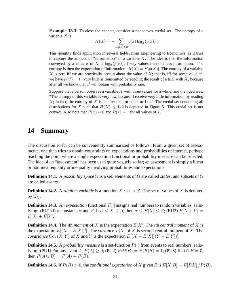
Example 13.3.To close the chapter, consider a nonconvex credal set. Theentropyof avariableX is

H(X) = −∑

x:p(x)>0

p(x) log2 (p(x)) .

This quantity finds application in several fields, from Engineering to Economics, as it triesto capture the amount of “information” in a variableX. The idea is that the informationconveyed by a valuex of X is log2 (p(x)): likely values transmit less information. Theentropy is then the expectation of information:H(X) = E[p(X)]. The entropy of a variableX is zero iff we are practically certain about the value ofX; that is, iff for some valuex′,we havep(x′) = 1. Very little is transmitted by sending the result of a trial with X, becauseafter all we know thatx′ will obtain with probability one.

Suppose that a person observes a variableX with three values for a while, and then declares:“The entropy of this variable is very low, because I receive very little information by readingX; in fact, the entropy ofX is smaller than or equal to1/2.” The credal set containing alldistributions forX such thatH(X) ≤ 1/2 is depicted in Figure 5. This credal set is notconvex. Also note thatP (x) = 0 andP (x) = 1 for all values ofx.

14 Summary

The discussion so far can be conveniently summarized as follows. From a given set of assess-ments, one then tries to obtain constraints on expectationsand probabilities of interest, perhapsreaching the point where a single expectation functional orprobability measure can be selected.The idea of an “assessment” has been used quite vaguely so far; an assessment is simply a linearor nonlinear equality or inequality involving probabilities and expectations.

Definition 14.1. A possibility spaceΩ is a set; elements ofΩ are calledstates, and subsets ofΩare calledevents.

Definition 14.2. A random variableis a functionX : Ω → <. The set of values ofX is denotedby ΩX .

Definition 14.3. An expectationfunctionalE[·] assigns real numbers to random variables, satis-fying: (EU1) For constantsα andβ, if α ≤ X ≤ β, thenα ≤ E[X] ≤ β; (EU2) E[X + Y ] =E[X] + E[Y ].

Definition 14.4. Theith momentof X is the expectationE[X i].Theith central momentof X isthe expectationE[(X − E[X])i]. ThevarianceV [X] of X is second central moment ofX. ThecovarianceCov(X, Y ) of X andY is the expectationE[(X − E[X])(Y − E[Y ])].

Definition 14.5. A probability measureis a set-functionP (·) from events to real numbers, satis-fying: (PU1) For any eventA, P (A) ≥ 0; (PU2)P (Ω|B) = P (B|B) = 1; (PU3) If A ∩ B = ∅,thenP (A ∪ B) = P (A) + P (B).

Definition 14.6. If P (B) > 0, theconditional expectationof X givenB isE[X|B] = E[BX] /P (B).

31

Definition 14.7. If P (B) > 0, theconditional probabilityof A givenB isP (A|B) = P (A ∩ B) /P (B).

Definition 14.8. A credal setis a set of probability measures.Strict conditioningonly definesthe conditional credal setK givenB whenP (B) > 0; in this caseK is the set of all conditionalmeasuresP (·|B). Regular conditioning, or simplyconditioning, only defines the conditionalcredal setK given B whenP (B) > 0; in this caseK is the set of all conditional measuresP (·|B) such thatP (B) > 0.

Definition 14.9. The lower and upper expectations of variableX are respectivelyE[X] =infP∈K E[X] andE[X] = supP∈K E[X]; the lower andupperprobabilities of eventA are re-spectivelyP (A) = infP∈K P (A) andP (A) = supP∈K P (A).

Definition 14.10. Theconditional lowerandconditional upperexpectations of variableX giveneventB are respectivelyE[X|B] = infP∈K E[X|B] andE[X|B] = supP∈K E[X|B] wheneverK(X|B) is defined; theconditional upperandconditional lowerprobability of eventA giveneventB are respectivelyP (A|B) = infP∈K P (A|B) andP (A|B) = supP∈K P (A|B) wheneverK(X|B) is defined.

15 Bibliographic notes

Events and random variables are the basic concepts of probability theory. Detailed discussionsof these concepts can be found in several excellent textbooks [3, 18]. States are also calledelements, points, outcomes, configurations. Usually the term sample spaceis used for the set ofstates; the termpossibility spacehas been proposed by Walley [22] and seems a more accuratedescription. Possibility spaces should not be viewed as fixed objects; they are often revised(enlarged, reduced, modified) when analyzing a problem. Thetermrandom variableis somewhatunfortunate as any random variable is actually defined in very deterministic terms. Other possiblenames arerandom quantity[2], gamble[22] andbet[11].

The use of identical symbols for events and indicator functions has been pionereed by deFinetti [2]; a nice discussion of this issue is given by Pollard [20]. There is another conventionproposed by de Finetti that is quite appealing. His second convention is to use the same symbolPfor probability and for expectation; that is,P (X) denotes the expectation of variableX. Howeverappealing, this notation may be confusing when mixed withp(X) (for probability mass functionsand densities). For this reason it is not adopted here.

Axioms PU1-PU3 offer a standard approach to probability in finite spaces [3, 18]; axiomsEU1-EU2 are their obvious “expectation version” [23]. Theyare adopted here for any possibilityspace, finite or infinite. Textbooks usually introduce probability axioms first, and expectation isthen defined; here the order is reversed (as in de Finetti’s [2] and Whittle’s [23] books). Thereare many reasons to start with expectations. First, expectations are arguably more intuitive froma practical point of view (they are obviously representing averages). Second, the move to infi-nite spaces is relatively simple for expectations, but verycomplex for probabilities (particularly

32

when conditioning is discussed on infinite spaces). Finally, many applications deal just withexpectations, or are just interested in expectations.

The definition of conditioning follows the usual Kolmogorovian theory [3, 13]; that is, noconditioning on events of zero probability. It would be better to free conditioning from such anunpleasant constraint.

The three-prisoners problem is described in many articles and books [1, 19].

This text emphasizes the need to represent assessments thatdo not yield a single probabilitymeasure. In this case one must employ credal sets. Early advocacy for credal sets can be foundin work by Good [10], Kyburg [14], Dempster [4, 5], Shafer [21], and others. The most vocalearly proponent of general sets of probability measures wasLevi [16, 17], who proposed the termcredal stateto indicate a state of uncertainty that can only be translated into a set of probabilitymeasures. Work by Williams [24, 25, 26], Giron and Rios [9] and Huber [12] offered axiom-atizations of credal sets. Sets of probability measures were then adopted in the field of robustStatistics and in a number of approaches to uncertainty within the field of Artificial Intelligence.A solid foundation was concocted by Walley [22] and the theory has grown steadily since then.The device of baricentric coordinates appears already in Levi’s work [17] and is extensively usedin the literature; Lad offers a detailed discussion [15].

The terms “probability mass function” and “joint probability mass function” can be replacedby the more general termdensity[20, Chapter 3]. The presentation here follows a traditionalscheme where densities are used for distinct purposes [3].

The literature offers vast material on Markov, Chebyshev, and similar bounds [3, 18, 7],Frechet bounds [6] and Bonferroni bounds [8].

16 A few exercises

16.1 Two salesmen are trying to sell different products. Theprobability that the first salesmanwill not sell his products is 0.2. The probability that the second salesman will not sell hisproduct is 0.4. What is the probability that neither salesmen will sell anything? What is theprobability that both will sell something? What is the probability that exactly one will notsell anything?

16.2 There are four pairs of objects in a table. The first two pairs contain two spoons each.The third pair contains two pencils. A robot selects a pair, then takes the pair and selectsan object from the pair. The probability that any of the pairsis selected is 0.25, and theconditional probability that either object is selected given a pair is 0.5.

(a) Suppose the fourth pair contains a spoon and a pencil. What is the possibility space?What is the probability measure on the possibility space? Ifthe selected object is a

33

spoon, what is the probability that the other animal is a spoon as well?

(b) Suppose now the fourth pair of objects containseither a spoon and a pencilor twopencils. If the selected object is a spoon, what is the lower probability that the otherobject is a spoon as well?

16.3 A doctor has a client that may have a diseaseD. The doctor performs a testT that canbe positive (T+) or negative (T−). The test has sensitivity 90% (P (T + |D) = 0.9) andspecificity 90% (P (T − |Dc) = 0.9).

• From medical journals, the doctor assumes that 20% of the population have diseaseD. DetermineP (D|T+).

• Suppose the doctor does not have statistics about the population but thinks thatP (D)must be larger than 0.01 but smaller than 0.3. Determine the interval of values ofP (D|T+). Can the doctor establish the status of the client? Suppose the doctor usesthe interval [0.15, 0.25] forP (D); can he say something definite about the client?

16.4 Two dice are to be thrown; the possibility space contains the 36 possible outcomes. Denoteby W the number of pips turned up on the first die and byX the number of pips turned upon the second die. DefineY = W + X andZ = min(W, X).

• Suppose first all 36 possible outcomes are given equal probability, and determinep(Y ), p(Z), p(Y, Z) andp(Y |Z).

• Now suppose the 6 possible values ofZ are given equal probability, with no furtherassessments. What is the lower probabilityP (Y = 4|Z = 3)?

16.5 Consider a variableX with 3 possible valuesx1, x2 andx3, and suppose the followingassessments are given:p(x1) ≤ p(x2) ≤ p(x3); p(xi) ≥ 1/20 for i ∈ 1, 2, 3; andp(x3|x2 ∪ x3) ≤ 3/4. Show the credal set determined by these assessments in baricentriccoordinates. Obtain lower and upper bounds for the probability P (x1|x1 ∪ x2).

17 More exercises

17.1. Prove thatE[X + α] = E[X] + α for any real numberα.

17.2. Prove theTriangle Inequality:√

E[(X + Y )2] ≤√

E[X2] +√

E[Y 2].

(Hint: Note thatE[XY ] ≤ E[|XY |]; apply the Cauchy-Scharwz inequality to show thatE[(X + Y )2] ≤ E[X2] + 2

√

E[X2] E[Y 2] + E[Y 2] and then note that the last expressionis equal to(

√

E[X2] +√

E[Y 2])2.)

34

17.3. Show that for any two eventsA andB, the probability that exactly one of them will occur isP (A)+P (B)−2P (A ∩ B). Generalize: show that given any eventsBi, the probabilitythat exactly one of them obtains is

n∑

i=1

(−1)i+1iSi,n.

(Hint: use an induction argument inspired by the proof of Theorem 2.1 and take expecta-tions.)

17.4. Suppose thatn eventsBi are given together with assessmentsP (Bi) (and no other as-sessments). Prove the following bounds:

max

((

∑

i

P (Bi))

)

− (n − 1), 0

)

≤ P (∩ni=1Bi) ≤ min

iP (Bi) .

17.5. The Kullback-Leibler divergence between distributionsP andQ is

D(P, Q) =∑

x:Q(X=x)>0

P (X = x) logP (X = x)

Q(X = x).

Show thatD(P, Q) ≥ 0.(Hint: Use Jensen inequality.)

17.6. Suppose thatg(X) is a non-negative non-decreasing function; show that fort > 0,

P (|X| > t) ≤ E[g(|X|)]g(t)

. (28)

This is a generalization of the Markov inequality. Now consider a binary variableX withprobabilityP (X = 1) = t. Show that the Markov inequality is in fact an equality in thiscase. (That is, we cannot improve on Markov inequality without further assumptions onX.) Construct a variable for which the inequality in Expression (28) is an equality (forfixed t).

17.7. Suppose that variableX assumes integer values from0 to k. Show that

E[X] =k∑

i=0

P (X > i) . (29)

Now show:E[X] ≥∑k

i=0 P (X > i).(Hint: write X as a sum of indicator functions.)

35

References

[1] Gert de Cooman and Marco Zaffalon. Updating incomplete observations. InProceedingsof the Conference on Uncertainty in Artificial Intelligence, pages 142–150, San Francisco,California, 2003. Morgan Kaufmann.

[2] Bruno de Finetti.Theory of probability, vol. 1-2. Wiley, New York, 1974.

[3] M. H. DeGroot.Probability and Statistics. Addison-Wesley, 1986.

[4] A. P. Dempster. Upper and lower probabilities induced bya multivalued mapping.Annalsof Mathematical Statistics, 38:325–339, 1967.

[5] A. P. Dempster. A generalization of Bayesian inference.Journal Royal Statistical SocietyB, 30:205–247, 1968.

[6] M. Denuit, J. Dhaene, M. Goovaerts, and R. Kass.Actuarial Theory for Dependent Risks.John Wiley & Sons, Ltd, 2005.

[7] Luc Devroye, Laszlo Gyorfi, and Gabor Lugosi.A Probabilistic Theory of Pattern Recog-nition. Springer Verlag, New York, 1996.

[8] Janos Galambos and Italo Simonelli.Bonferroni-type inequalities with applications.Springer-Verlag, New York, 1996.

[9] F. J. Giron and S. Rios. Quasi-Bayesian behaviour: A morerealistic approach to decisionmaking? In J. M. Bernardo, J. H. DeGroot, D. V. Lindley, and A.F. M. Smith, editors,Bayesian Statistics, pages 17–38. University Press, Valencia, Spain, 1980.

[10] I. J. Good.Good Thinking: The Foundations of Probability and its Applications. Universityof Minnesota Press, Minneapolis, 1983.

[11] J. A. Hartigan.Bayes theory. Springer-Verlag, New York, 1983.

[12] P. J. Huber.Robust Statistics. Wiley, New York, 1980.

[13] Andrei Nikolaevich Kolmogorov.Foundations of the theory of probability. Chelsea Pub.Co. (translation edited by Nathan Morrison, original from 1933), New York, 1950.

[14] H. E. Kyburg Jr. The Logical Foundations of Statistical Inference. D. Reidel PublishingCompany, New York, 1974.

[15] Frank Lad.Operational subjective statistical methods: a mathematical, philosophical, andhistorical, and introduction. John Wiley, New York, 1996.

[16] Isaac Levi. On indeterminate probabilities.Journal of Philosophy, 71:391–418, 1874.

[17] Isaac Levi.The Enterprise of Knowledge. MIT Press, Cambridge, Massachusetts, 1980.

36

[18] A. Papoulis. Probabilities, Random Variables and Stochastic Processes. McGraw-Hill,New York, 1991.

[19] J. Pearl.Probabilistic Reasoning in Intelligent Systems: Networksof Plausible Inference.Morgan Kaufmann, San Mateo, California, 1988.

[20] David Pollard. A User’s Guide to Measure Theoretic Probability. Cambridge UniversityPress, 2001.

[21] G. Shafer.A Mathematical Theory of Evidence. Princeton University Press, 1976.

[22] P. Walley.Statistical Reasoning with Imprecise Probabilities. Chapman and Hall, London,1991.

[23] Peter Whittle.Probability. Penguin, Harmondsworth, 1970.

[24] P. M. Williams. Coherence, strict coherence and zero probabilities.Fifth Int. Congress ofLogic, Methodology and Philos. Sci., VI:29–30, 1975.

[25] P. M. Williams. Notes on conditional previsions. Technical report, School of Math. andPhys. Sci., University of Sussex, 1975.

[26] P. M. Williams. Indeterminate probabilities.Formal Methods in the Methodology of Em-pirical Sciences, 1976.

37