A Few Bad Apples: An Analysis of CEO Performance Pay and Firm Productivity*

October 2009

Laarni Bulan**

Paroma Sanyal

Zhipeng Yan

Abstract

We investigate the relationship between CEO performance pay incentives and firm productivity. In general, we find an inverse U-shaped relationship between productivity and the sensitivity of CEO wealth to share value (delta) and a positive relationship between productivity and the sensitivity of CEO option wealth to stock return volatility (vega). Thus, a high delta associated with CEO risk-aversion lowers productivity, but a high vega from stock options offsets this effect. In looking at delta and vega jointly, we also find that options do not always achieve their intended purpose. These results are stronger among firms that are weakly governed or when high transaction costs prevent the writing of an optimal compensation contract.

JEL codes: G32, G30, L2, O3 Keywords: CEO, Executive Compensation, Pay-for-Performance Sensitivity, Productivity

*Bulan and Sanyal: Brandeis University, International Business School and Economics Department, 415 South Street, MS 021, Waltham, MA 02454. Yan: New Jersey Institute of Technology, School of Management, University Heights, Newark, NJ 07102. This paper has benefitted tremendously from the comments and suggestions of an anonymous referee. We also are grateful to Susan Athey, Susanto Basu, Audra Boone, Johannes Van Biesebroeck, Alex Edmans, Ravi Jain, Blake Le Baron, Hong Li, Hamid Mehran, Rachel McCulloch, Carol Osler, Carsten Pohl, Bob Reitano, Narayanan Subramanian and seminar participants at Brandeis University, Northeastern University, the NBER productivity group, the NBER Productivity Summer Workshop 2007, the FMA 2006 Annual Meeting, the 2007 IIOC Annual Meeting and the MFA 2007 Annual Meeting for helpful comments. All errors and omissions are our responsibility. ** Corresponding author, lbulan@brandeis.edu Phone: 781-736-2994.

0

“Shareholders have woken up to the perverse effects on executive behavior of corporate pay, and especially of stock options, and want to see pay more directly linked to performance.” -- The Economist, April 15th, 2004 “Indeed, the story behind the growth of pay in the 1990s is really the story of the option.” -- The Economist, January 18th, 2007

1. Introduction

The corporate scandals early in this decade prompted vast reforms in the setting of

executive pay in the U.S. New Securities and Exchange Commission (SEC) rules for greater

transparency in executive pay were implemented in 2007. As early as 2003, surveys1 had shown

that CEO pay shifted away from stock options and into restricted stock grants as a means of

rewarding good performance. Stock options have long been viewed as an effective tool for

aligning CEO incentives with those of shareholders. These corporate scandals have put

executive stock options in a bad light. We argue that the shift away from options in CEO pay is

not necessarily the solution. It is the combination of both restricted stock and stock option

grants, or the total equity-linked component of pay, that affect CEO incentives.2 In a sample of

U.S. manufacturing firms over the period 1992-2003, we find that for the vast majority of firms,

CEO pay-for-performance incentives positively impacted the real-side of firm performance, as

measured by total factor productivity (or TFP). It is only for a small fraction of firms in our

sample that the CEO’s equity-linked compensation was ineffective.

Existing work has mainly focused on the relationship between executive compensation

and firm financial performance. We argue that firm productivity is an equally important measure

1 “A Better Option,” The Economist, April 15, 2004. 2 This is analogous to Mehran (1995) who argues that “the form rather than the level of compensation is what motivates managers to increase firm value.” See also Johnson, Ryan and Tian (2009). We focus on stock and stock options since these represent the largest portion of CEO pay in our sample.

1

of performance that is often overlooked.3 Studies have shown productivity growth to be

associated with long-run economic growth, standard of living, inflation and economic welfare.4

Our analysis in particular includes a period of rapid U.S. productivity growth in the 1990s. This

rapid growth has been attributed mainly to technological improvements (Basu, Fernald, and

Shapiro (2001)). Similar growth rates in productivity were last seen in the US in the 1950s and

1960s. Hence, explaining this phenomenon has significant policy implications.

Our results suggest that CEO stock and stock option grants contributed to the growth in

productivity in the 1990s. CEO incentive contracts shifted towards stock and stock option grants

beginning in the 1980s (Murphy (1999), Perry and Zenner (2000)). In particular, Hall and

Liebman (1998) show that stock option grants dramatically increased both the level of CEO

compensation and the sensitivity of CEO compensation to firm performance in the 1990s

compared to the 1980s. Figure 1 shows how this shift in compensation strategies may have

contributed to the growth in productivity. Moreover, not only did the growth in productivity and

the growth in CEO compensation coincide, but also in 2001-2002, both productivity and CEO

compensation declined, suggesting a systematic relationship between firm productivity and CEO

compensation incentives.

Our focus on productivity is further driven by the need to identify the channels through

which managerial incentives influence firm financial performance (e.g. profitability or stock

return performance). Productivity is perhaps the most important channel through which

managers can improve a firm’s long-term financial performance since improvements in

productivity are more permanent. Recognizing this, some compensation committee reports have

3 To the best of our knowledge, the exception is Palia and Lichtenberg (1999) who investigate the relationship between productivity and managerial stock holdings during the period 1982-1993. We discuss in greater detail the contributions of our study relative to existing work in section 2. 4 See Steindel and Stiroh (2001) and Basu and Fernald (2002).

2

stated goals and performance targets for the CEO where productivity enhancement is an

explicitly-stated objective.5 Bartelsman and Doms (2000) argue that a firm’s choice of

innovative activity is a fundamental factor that affects productivity. Thus, CEO decisions related

to investment in research and development (R&D), patenting activity, and technology adoption

for example, are crucial in enhancing firm productivity.6

In this paper, we first establish a link between productivity and financial performance.

Having established this link, we investigate whether CEO incentives are effective in aligning

managerial objectives with shareholders’ productivity enhancement goals. From our empirical

model we find a strong positive relationship between a firm’s financial performance, as

measured by Tobin’s q, and total factor productivity at the firm level. Thus increasing

productivity is ultimately reflected in firm value, whether or not productivity enhancement is an

explicitly stated objective for the CEO.

Next, we examine how various components of CEO compensation affect productivity.

First, we show that the sensitivity of CEO wealth to percent changes in his firm’s stock price

(“delta”) has a significant influence on productivity. Incentives between CEOs and shareholders

become better aligned as delta increases leading to higher firm productivity. However, CEOs

with high delta have an adverse impact on firm productivity suggesting that they are averse to

taking on more risk as the value of their portfolios become very sensitive to small changes in

their firm’s stock price. Thus, we find that productivity has an inverted U-shaped relationship

with CEO delta.

5 We refer the reader to Bushman, Indjejikian and Smith (1996) for specific examples of compensation committee reports. They document that, in practice, intermediate measures of firm performance (as opposed to just financial or accounting criteria) are also used in the determination of CEO incentive plans. 6Aghion, Van Reenen and Zingales (2009) develop a theoretical model where the CEO is faced with the decision to pursue risky innovation strategies at the expense of possible termination due to project failure.

3

Second, we investigate whether the sensitivity of CEO wealth to percent changes in stock

return volatility (“vega”) enhances productivity. Vega is a measure of the risk-taking incentive

from stock option grants. Risk-averse CEOs may be more willing to undertake riskier but

productivity enhancing projects since option values increase with firm risk.7 We find that in

general, this risk-taking incentive from stock option grants has a positive impact on productivity.

Last, in looking at delta and vega jointly, we find that there are instances when options do

not always achieve their intended purpose, i.e. to make managers more willing to take risk, at

least in terms of productivity. We find that for a range of delta values where CEO risk-aversion

is not a concern, a higher vega reduces productivity: a result that has not been previously

documented to our knowledge.8

Encouragingly, for the vast majority of firms in our sample, CEO compensation contracts

were mostly effective in enhancing the real-side of firm performance. We further investigate the

mechanisms that could be driving our results and find that the complex relationship between

productivity and CEO incentives is stronger among weakly governed firms and among firms

where transaction costs prevent the writing of an optimal compensation contract.

Our findings highlight the importance of careful structuring of CEO compensation

contracts. We find that appropriate combinations of CEO stock and stock option grants are

positively related to his firm’s productivity. These results thus question the move out of stock

options and into restricted stock grants in CEO pay in response to the corporate scandals earlier

in this decade.

7 Dittmann and Yu (2008) find that providing risk-taking incentives is particularly relevant in their sample of U.S. CEOs. 8 We uncover this result by looking at the joint effect of delta and vega (i.e. the interaction between these two measures) on productivity. Existing work in this area has mainly focused either on delta or vega only. The exceptions that we are aware of are Guay (1999), Habib and Ljungqvist (2005), Coles, Daniel and Naveen (2006) and Chakraborty, Sheikh, and Subramanian (2007). We thank Alex Edmans for making this observation.

4

The remainder of the paper is organized as follows: Section 2 reviews previous work and

discusses where our paper fits into the existing literature. Section 3 describes our data and the

variables used in our analysis. Section 4 shows that productivity is positively related to Tobin’s

q. Section 5 explains our empirical methodology. Section 6 discusses our results and Section 7

concludes.

2. Related Literature

The existing theoretical literature suggests that CEO ownership, or specifically the share

of a corporation owned by the CEO, has multiple influences on firm performance (Berle and

Means (1935), Jensen and Meckling (1976), Demsetz (1983), Fama and Jensen (1983), Smith

and Stulz (1985)). On the positive side, when CEOs own more shares of their firm, they benefit

more from value-maximizing decisions since these result in share-price increases (incentive-

alignment effect). However, when CEOs own a large fraction of corporate shares they can

become “entrenched,” i.e. independently powerful and difficult to dislodge. In this case, he may

attempt to benefit himself at the expense of less powerful shareholders (entrenchment effect).

This could create an inverse U-shaped relationship between CEO ownership and corporate

performance. In addition, when CEOs own a large absolute amount of corporate shares they

become more exposed to share-price volatility (or risk) directly and indirectly, insofar as their

portfolios become less diversified. This will concern risk-averse CEOs who may forgo risky yet

value-enhancing projects (risk-aversion effect).

Given these multiple influences, it is not surprising that the empirical literature has not

reached a consensus regarding the relationship between managerial ownership and corporate

performance, which is typically measured as Tobin’s q. The earliest papers that have linked

5

managerial ownership to Tobin’s q found that the relationship is non-linear and essentially has an

inverse U-shape (Morck, Shleifer and Vishny (1988), McConnell and Servaes (1990)). These

studies suffer, however, from the potential endogeneity of ownership (Himmelberg, Hubbard and

Palia (1999), Palia (2001)). More recent studies attempt to address the endogeneity problem by

using instruments for ownership or by using simultaneous equation estimation, with mixed

results.9 We circumvent this estimation issue by first relating productivity to Tobin’s q and then

relating CEO incentives to productivity. In so doing, we trace the effects of CEO incentives to

Tobin’s q and show that productivity is an important channel through which managerial

incentives affect firm financial performance.

On the issue of CEO risk-aversion due to CEO portfolio risk arising from high delta,

stock options have been proposed as the solution. Haugen and Senbet (1981) show that the use of

executive stock options may encourage CEOs to make riskier investment choices due to the

added convexity (vega) in compensation structures. On the other hand, Ross (2004) shows that

under certain conditions, adding call options to a manager’s compensation package also

increases the delta and can actually make a manager more risk-averse, contrary to conventional

wisdom. Empirical studies have documented that the use of options is related to riskier corporate

decisions. One such paper that is closely related to ours is Coles, Daniel and Naveen (2006).10

Their paper examines the relationship between managerial incentives and specific firm policies

on capital expenditures, research and development (R&D) and leverage. They find that higher

CEO vega results in riskier firm policies (lower capital expenditures, higher R&D and higher

leverage). While Coles, Daniel and Naveen show that CEO compensation in the form of stock

9 Hermalin and Weisbach (1991), Loderer and Martin (1997), Cho (1998), Himmelberg, Hubbard and Palia (1999), Holderness, Kroszner, and Sheehan (1999), Demsetz and Villalonga (2001), Palia (2001), Claessens, Djankov, Fan and Lang (2002), Cui and Mak (2002), Habib and Ljungqvist (2005), Brick, Palia and Wang (2005). Coles, Lemmon and Meschke (2007) adopt a structural approach to address this endogeneity problem. 10 Other papers include Guay (1999) and Rogers (2002).

6

options induces risk-taking behavior, we investigate whether this riskier behavior positively

affects firm performance. Our results suggest that when we look at the real-side of firm

performance, this riskier behavior results in higher productivity for most of the firms in our

sample. Since productivity is significantly and positively related to firm value, we argue that

option contracts are largely effective in aligning CEO interests with those of the shareholders.

However, we also find that in a few instances where CEO risk-aversion is not a concern,

increasing vega results in lower productivity. Under these circumstances, we view this result as

being consistent with Ross (2004) in that adding stock options make CEOs more risk-averse

which results in under-investment (forgoing risky yet positive-NPV or productivity-enhancing

projects). An alternative interpretation is related to Peng and Röell (2008), who find that

executive stock options can create incentives for managers to focus on the short term stock price.

This kind of myopic behavior could crowd out efforts directed at improving productivity.

On the issue of productivity and managerial incentives, the paper closest in spirit to ours

is Palia and Lichtenberg (1999)11. They estimate a production function with labor and capital as

factor inputs where the productivity parameter is a function of managerial ownership. To address

endogeneity concerns in the estimation of the production function, they employ a fixed effects

methodology and use lagged values of factor inputs and managerial ownership. From a randomly

selected sample of 255 US manufacturing firms over the period 1982-1993, they find that

changes in the equity holdings of managers are positively related to changes in productivity. Our

paper builds on their paper, but differs in two important ways. First, we use measures of CEO

incentives that better reflect current compensation contracts and are more closely tied to firm

performance. Palia and Lichtenberg look solely at managerial ownership and find that increasing

11Other related papers include the following: Barth, Gulbrandsen and Schøne (2005), Köke and Renneboog (2003), Nickell, Nicolitsas and Dryden (1997) and Perez-Gonzales (2004).

7

the equity holdings of managers increase firm productivity. Our sample period covers the 1990s

when the use of executive stock options became quite prevalent. We believe that CEO equity

ownership is an incomplete measure of a CEO’s pay-for-performance incentives for our time

frame. We find that more nuanced incentive measures, i.e. the CEO’s delta and vega, that

capture the multiple influences of stock and stock options on CEO behavior, better explain firm

productivity. A second difference is our use of a productivity estimation methodology that better

corrects for the endogeneity of the capital stock and selection issues due to firm exit. We discuss

our choice of methodology in greater detail in section 5.

3. Data and Variable Construction

We gather data from two main sources. We obtain annual CEO compensation data from

ExecuComp for the period 1992-2003. We obtain firm characteristics from Compustat. We focus

exclusively on manufacturing firms, for which our productivity estimation is likely to be most

reliable. Our sample comprises all 917 of the manufacturing firms represented in both

ExecuComp and Compustat with no missing observations for certain key variables.12 Because

ExecuComp focuses on major firms, such as the S&P 1500, our sample is dominated by large

firms.13 Our primary sample consists of 6,636 firm-year observations.

3.1 Measuring CEO Incentives

12 These variables are productivity, lagged productivity, total assets, firm age and CEO share holdings. 13 In a recent paper, Cadman, Klasa and Matsunaga (2007) document some systematic differences between ExecuComp and non-ExecuComp firms. They find that increasing the heterogeneity of the sample by including non-ExecuComp firms “uncover(s) previously hidden conditional or nonlinear relations.” We acknowledge that our use of ExecuComp firms may weaken the generality of our findings. On the other hand, our results already indicate a non-linear relation between firm productivity and CEO performance incentives, so that the “biases” that these authors document may not be as severe for this study.

8

We use two measures of CEO incentives that are widely used in the literature and that are

closely tied to firm performance. These are delta, the sensitivity of CEO wealth to percent

changes in the firm’s share price, and vega, the sensitivity of CEO wealth to percent changes in

stock return volatility. Delta is measured as the dollar change in the CEO’s equity and option

holdings in response to a one-percent change in the firm’s stock price. Vega is measured as the

dollar change in the CEO’s option holdings in response to a one-percent change in the firm’s

stock return volatility. More specifically,

CEO delta = Equity delta + Option delta (or Equity delta if Option delta is missing) (1)

Equity delta = (2) 01.0*P/ueequity val P

= (3) 01.0*PN S

Option delta = (4) 01.0*/ueoption val1

PPON

jj

CEO vega = (5) 01.0*/ueoption val1

ON

jj

where Ns and No are the number of shares and number of options, respectively, held by

the CEO, P is the stock price and σ is the stock return volatility. Option value for each grant j is

calculated using the Black-Scholes (1973) formula for European call options modified for

dividend paying stocks (Merton (1973). We follow prior work and use the Core and Guay

(2002) methodology for estimating option delta and vega. The vega of option holdings has been

shown by Guay (1999) to be of an order of magnitude larger than the vega of stock holdings.

9

Hence we approximate the CEO’s vega to be the vega from option holdings.14 We provide the

details of these calculations in Appendix B. To our knowledge, these measures have not

previously been linked to productivity.

Delta and vega are also referred to as the slope and convexity, respectively, of the CEO

wealth-performance relation (compensation contract).15 The slope (delta) is a measure of

incentive-alignment, i.e. CEO incentives become more aligned with shareholder goals as the

slope increases. However, CEO risk-aversion is often associated with steeper slopes (high levels

of delta). Convexity (vega) measures the risk-taking incentive generated by stock option grants.

Guay (1999) argues that shareholders need to manage both the slope and the convexity of the

CEO’s wealth-performance relation in order to induce managers to make optimal investment and

financing decisions.

While the focus of this paper is on the incentives generated by the equity-linked

components of CEO pay, we also control for CEO cash compensation since studies suggest it

may be related to firm productivity.16 We measure cash compensation as the sum of the CEO’s

base salary and annual bonus. Base salary is the fixed component of CEO pay that modestly

increases from year to year. It is usually benchmarked at the industry level and has been

documented to be highly correlated with firm size, especially for firms that have strong stock

return performance. Annual bonus is calculated as a percentage of base salary and is very often

tied to short term firm performance (e.g. if certain targets for accounting profitability are met for

the year). Thus, although a CEO’s cash compensation is more likely to create short-term

incentives, it may be correlated with firm productivity to the extent that the bonus is related to

14 Coles, Daniel and Naveen (2006), among others, follow the Core and Guay methodology and also make this same approximation. 15Jensen and Meckling (1976), Haugen and Senbet (1981), Smith and Stulz (1985), Milgrom and Roberts (1992) 16 See Murphy (1999). We thank an anonymous referee for this suggestion.

10

financial performance. Furthermore, the competitive labor market for CEOs is likely to result in

salary levels that are strongly linked to firm performance (Leone, Wu and Zimmerman (2006)).

On the other hand, cash compensation is also perceived to be related to risk. Coles, Daniel and

Naveen (2006) use CEO cash compensation as a proxy for CEO risk aversion. They argue that

either: (1) Managers with high cash compensation are more likely to be entrenched (high

ownership levels) and hence would be more risk averse (Berger, et al. (1997)), or (2) CEOs with

higher cash compensation are more diversified since they have greater wealth to invest outside

their own firm, and hence are less risk averse (Guay (1999)).

3.2 Estimating Total Factor Productivity

Total factor productivity or TFP is the conventional measure of firm-level productivity.

TFP is defined as the amount of output that cannot be explained by the corresponding factor

inputs. Consider that firms have idiosyncratic efficiencies but face the same market structure and

factor prices. Firms produce output (y) using a fixed factor, capital (k), and a variable input such

as labor (l), as given by the (log-linear) Cobb-Douglas production function below.

itititkitlit kly 0 (6)

In this equation, ωit is the efficiency (productivity) parameter that is unobserved by the

econometrician but known by the firm when making investment and staffing decisions. εit is the

idiosyncratic error term. Estimation of the production function needs to address the following

issues: 1) endogeneity of inputs, due to unobservable firm heterogeneity and because the capital

stock is correlated with productivity through past productivity, and 2) selection bias because of

firm exit, which may occur due to a negative productivity shock.

11

Olley and Pakes (1996) developed a methodology that addresses these issues.17 We

follow this procedure to estimate the production function. Since the underlying production

function parameters may be different across industries, we estimate the production function

separately for each industry group following the Fama-French 49 industry classification. TFP is

then calculated as the difference between actual and predicted output. Appendix A describes this

estimation procedure in greater detail.

The measurement of TFP as the difference between actual and predicted output has its

origins from Solow (1957). The Solow model in essence defines a change in TFP as a shift in the

production function (a change in the Cobb-Douglas technology parameter). Thus, given the same

factor inputs (capital and labor), an increase in TFP denotes a shift in the production function

that increases firm efficiency. Based on this interpretation, the two most commonly identified

sources of productivity gains are changes in technology and unobserved efficiency increases.

The latter can include factors such as managerial efficiency.18 For the former, Basu, et al. (2001)

show that technological change is a dominant factor that explains the productivity growth in our

sample period.

To make our TFP estimates comparable across industries, we compute a productivity

index (Pavcnik (2002), Aw, et. al (2001)) as follows: We consider 1992 to be the base year for

which we calculate the mean TFP estimate by industry group. We then subtract this 1992

industry mean from firm-level TFP to obtain the productivity index: pindxit=prodv_estit –

prodv_estj,1992, where j is the industry group of firm i and t denotes the current year. In the

regression analysis that follows, we use this productivity index as the dependent variable. (Table

17 Another advantage of this methodology is that it is robust to a variety of estimation issues. Its shortcoming is that its estimates can be quite sensitive to measurement error in investment (Van Biesebroeck (2007)). In this paper, investment is measured as capital expenditures (in property, plant and equipment). Since this is a flow variable that is reported by firms each year, we believe measurement problems are not that severe. 18 Bartelsman and Doms (2000) discuss various factors that could affect firm-level productivity.

12

A2 provides descriptive statistics for this index while Figure 1 shows how the index changes

over time.)

3.3 Measuring Firm Characteristics

To evaluate the contribution of CEO incentives to productivity, it is important to control

for other important factors. Following previous work, we require the following additional

factors in our analysis: firm size (total assets), firm age, industry concentration (Herfindahl

index), Tobin’s q, sales, tangible assets, capital expenditures, book leverage, stock return

volatility, research and development, advertising, and CEO tenure. Further details on the

measurement and construction of these variables are outlined in Appendix B.

Table 1A reports descriptive statistics for our estimation sample. For a majority of the

observations, CEOs own less than 0.5 percent of their firm’s stock. However, this distribution is

heavily skewed since the mean equity stake is 2.81 percent. The patterns for delta are similar to

that of equity holdings. A one percent increase in the firm’s stock price results in a median

increase in CEO wealth of $180,000, while the mean increase is $540,000. With regards to vega,

a one percent increase in the volatility of a firm’s stock return corresponds to a median (mean)

increase in CEO wealth of $30,000 ($80,000). In Table 1B, we report the correlation matrix for

our variable set.

4. Productivity and Financial Performance

The stated objective of a CEO is to maximize shareholder value. However, without

fundamental changes to underlying productivity, sustained improvements in financial

performance (share value) will not be possible. Thus, we first document how productivity and a

firm’s financial performance are related. Figure 1 shows that the productivity surge of the 1990s

13

coincided with the large increase in CEO pay. Moreover, it is also the case that the stock market

reached unprecedented heights over this same time period. This begs the question of whether

these productivity gains translate into enhanced corporate value. We argue that productivity is

an important, and often overlooked, channel through which a firm’s financial performance is

affected. Ultimately, a CEO’s motivation for increasing firm productivity is to increase

shareholder value. This is an important link to establish, since one may argue that with a

relatively short average tenure, CEOs may not be interested in investing resources to increase

productivity, which is typically difficult to measure and may not be immediately reflected in

stock prices. However, if productivity is valued correctly and reflected in the market valuation of

the firm, then irrespective of their expected tenure horizons, CEOs would have an incentive to

invest in productivity enhancements.

Following previous work, we use Tobin’s q as a market-based measure of the firm’s

financial performance. We measure productivity here as the estimated productivity residual from

the production function (equation 6), rather than the productivity index that we use as a

dependent variable in subsequent analysis. This is because we want to relate the firm’s actual

TFP estimate, which is the residual, to its market valuation. Our results are unchanged if we use

the productivity index instead of the residual. We control for the influence of various additional

determinants of Tobin’s q that have been identified by prior studies (Himmelberg, Hubbard and

Palia (1999)) such as firm size, tangible assets, investment, industry concentration, R&D,

advertising, leverage and stock return volatility. We use a firm fixed effects methodology to

estimate this empirical specification. The results in Table 2 show that productivity has a highly

significant, positive impact on Tobin’s q even after controlling for these other influences.19 This

supports our analysis of the real-side of firm performance as it ultimately affects a firm’s 19 Palia and Lichtenberg (1999) and Schoar (2002) also find that Tobin’s q is positively related to productivity.

14

financial performance which shareholders care about. Moreover, as we have previously argued,

we expect productivity improvements to be more permanent and hence have a lasting impact on

a firm’s share price.

5. Estimating the Productivity-Incentives Relationship

We now examine the incentive structure of CEO equity-based pay and its impact on

productivity. We find that equity ownership alone does not adequately capture the relationship

between CEO pay-for-performance incentives and productivity. Instead, we find that a CEO’s

delta and vega positively impact productivity for the vast majority of firms in our sample, but

that this relationship is non-linear and quite complex. Thus, appropriate combinations of delta

and vega must be chosen in order to align CEO incentives with the goal of productivity

improvement.

5.1 Benchmarking our Specification

We begin by estimating a production function with firm and year fixed effects, similar to

Palia and Lichtenberg (1999). The inputs to production are labor and capital while the

productivity parameter (TFP) is a function of managerial effort as proxied by lagged values of

CEO holdings (stock ownership). Following Palia and Lichtenberg, we estimate linear, quadratic

and cubic functional forms for CEO ownership.20 Table 3 shows that CEO stock ownership is

insignificant in this specification. When we replace CEO ownership with CEO delta in column 4

we find CEO delta is significant with a cubic functional form. Thus, the complex nature of

20 Here, we exclude CEO cash compensation in order to directly compare our results to those of Palia and Lichtenberg (1999).

15

compensation contracts prevalent in the 1990s calls for more nuanced measures of CEO

incentives that are more closely aligned with firm performance.

In our preferred specification, we do not include CEO incentives directly in the

production function for two reasons. First, efficient estimation of the production function using a

linear fixed effects technique is often problematic due to the endogeneity of factor inputs

(especially capital) and selection issues due to firm exit. Second, managerial effort is affected by

various parts of the compensation contract (delta and vega) and using these as separate inputs to

the production function belies their complexity. Thus our preferred approach is to first estimate

total factor productivity using a two-factor Olley-Pakes (1996) methodology, and then relate TFP

to CEO incentives.

We estimate the following empirical model:

ittiitit ControlsIncentives CEO Prod Prod 10it0it , (7)

The dependent variable is the productivity index previously described. CEO Incentives consists

of CEO delta and vega and CEO cash compensation, i is a firm fixed effect for firm i, t is a

year fixed effect for year t, and it is the error term. We include the lagged productivity index to

account for the persistence of productivity over time, i.e. our model has a first order

autoregressive structure.

There is a large literature that has identified important factors that influence firm-level

productivity and we draw our Controls from this literature. The basic factors that we use are:

firm size (Soderbom and Teal (2001)), firm age (Huergo and Jaumandreu (2004), Haltiwanger et.

al. (1999)), industry structure and competition measured by an industry concentration index

16

(Tang and Wang (2005), Rogers (2004)) and research and development expenditures (Griliches

(1986), (1980), Griliches and Lichtenberg (1984)).21

5.2 Methodological Issues

To determine the relationship between productivity and CEO performance pay

incentives, we face two estimation issues. First, is the endogeneity of CEO incentives, and

second, is the persistence of productivity shocks. The widely-recognized endogeneity problem

in estimating the relationship between financial performance and managerial compensation is

generally attributed to unobservable firm heterogeneity or differences in the firm’s contracting

environment.22 The firm’s level of technology is an unobservable factor and prior work

suggests that endogeneity in the relationship between firm productivity and CEO performance

pay incentives will largely be driven by differences in technology during our sample period.23

More specifically, firms with a superior technology, ceteris paribus, are more productive. At the

same time, however, having the superior technology also means that less incentive alignment (a

smaller delta) and/or less risk-taking incentives (a smaller vega) are required to ensure that this

firm’s CEO will pursue (risky) productivity-enhancing endeavors. This unobservable

heterogeneity, if not sufficiently addressed, is likely to affect our results.

Another potential source of endogeneity is the effect of past performance on current CEO

compensation. To a certain extent, CEO contracts reflect how the firm performed in the recent

past. For example, new equity or option grants may be awarded when incentives become mis-

21 To preserve sample size, we follow Himmelberg, Hubbard and Palia (1999) and include a dummy variable to account for missing values of R&D. This dummy variable equals 1 if R&D is non-missing. Missing values of R&D are replaced with zeros. One-fifth of our sample has missing R&D data. 22 See Demsetz (1983), Jensen and Warner (1988), Himmelberg, Hubbard and Palia (1999), Palia (2001). 23 For example, Basu, Fernald and Shapiro (2001) attribute the productivity growth in the 1990s to improvements in technology.

17

aligned due to recent stock price changes.24 In fact, Core and Guay (1999) find that firms award

new stock and stock option grants to (re-)optimize CEO incentive levels. The autoregressive

structure of our empirical model helps to address this issue: lagged TFP controls for some of the

bias arising from the effect of past firm performance on current CEO compensation.

If we appropriately address these endogeneity problems and optimal contracts are

awarded to CEOs, then we should not observe a systematic relationship between productivity

and CEO incentives since both productivity and CEO contracts are determined by unobservable

firm-specific factors. On the other hand, if transaction costs25 inhibit optimal contracting, then

we would observe a systematic relationship between CEO incentives and productivity.26 We

have argued that productivity is not as readily observable as financial performance measures.

Thus, writing contracts on productivity and enforcing such contracts can be rather costly. The

more common alternative is to write contracts on financial performance. Furthermore,

Holmstrom and Milgrom (1991) show that compensation contracts that are primarily based on

observable performance targets (e.g. financial targets) may be ineffective with respect to other

performance measures that are not easily measured or observed, such as total factor

productivity.27 Thus, we expect to find a systematic relationship between firm productivity and

CEO incentives even after accounting for endogeneity problems.

We use the difference-GMM estimator according to Arellano and Bond (1991) to address

the aforementioned estimation issues. This is an instrumental-variables procedure that not only

controls for firm fixed effects but also provides consistent and efficient coefficient estimates in

24 We thank an anonymous referee for pointing this out. 25 Tirole (1999) reviews the incomplete contracting literature and categorizes transaction costs into: 1) unforeseen contingencies, 2) the cost of writing contracts, and 3) the cost of enforcing contracts. 26 See Agrawal and Knoeber (1996) and Palia (2001). 27 Hall and Murphy (2000, 2002) and Hall (2003) also argue that managers value their stock and stock option grants at a discount relative to the cost of these grants to the shareholders. This value/cost discount ranges from 20% to 60% for standard at-the-money option grants – an inefficiency that represents a significant transaction cost as well. We thank an anonymous referee for this observation.

18

the presence of a lagged dependent variable (dynamic panel data estimator). As a GMM

estimator, this methodology can address endogeneity concerns with an appropriate set of

instruments. Unlike instrumental variable-fixed effects (IVFE) estimation, difference-GMM does

not require strict exogeneity of instruments, i.e. instruments need only be predetermined or

weakly exogenous. The set of valid instruments contains lagged values of the explanatory

variables, which includes twice-lagged productivity. Hence, an added advantage of this

instrumental variables approach is that it captures some of the direct effects of past productivity

levels on CEO compensation. Over-all, the Arellano-Bond methodology corrects for the two

estimation issues we face, i.e. the endogeneity of CEO compensation and the persistence of

productivity shocks which cannot both be addressed by standard IVFE models used in prior

work. Appendix C describes the Arellano-Bond methodology in greater detail.

We rely on previous literature to identify variables for our instrument set: firm size, firm

age, CEO tenure, stock return volatility, R&D, advertising, and book leverage. We use the

lagged values of these factors as instruments for CEO incentives.28 The justification for these

instruments are well-articulated by Core and Guay (1999), Himmelberg, Hubbard and Palia

(1999) and Palia (2001) and we summarize their arguments in Appendix D. We report two

specification tests to ensure their validity: 1) the Hansen J test for over-identifying restrictions;

and 2) the Arellano-Bond m2 test for lack of serial correlation in the error term it. This latter test

is important because of the lagged dependent variable in our model. For both tests, p-values of

less than 10 % would mean a rejection of the validity of the instruments at conventional levels of

significance.

28 Firm size and firm age are also control variables in our specification.

19

5.3 Alternative Specifications

In Table 4, we first estimate our empirical model using pooled ordinary least-squares

(OLS) and firm fixed effects estimation (columns 1 and 2). In these specifications, we use

lagged CEO delta and lagged CEO cash compensation to mitigate some of the endogeneity

concerns between productivity and CEO incentives. Both the pooled OLS and fixed effects

models yield insignificant coefficients on CEO delta while cash compensation has a significant

positive coefficient.

We believe firm fixed effects estimation is insufficient to adequately address the

endogeneity problem here because our sample period includes a time of rapid technological

change. To account for endogeneity problems and TFP persistence in a consistent manner, we

use the difference-GMM estimator (column 3).29 Of course, we do not expect to fully address the

issue of endogeneity. However, we are confident that estimation biases are minimized in our

analysis. This is evidenced by the fact that both the Hansen J test and the m2 test indicate that our

model is not mis-specified and the validity of our instruments is not rejected. We now turn to the

interpretation of the variable coefficients for the difference-GMM results.

6. Results

6.1 Lagged Productivity and Controls

From Table 4 (column 3) the coefficient on lagged productivity is positive and highly

significant, consistent with our priors regarding the persistence of productivity. This result is

consistently found in all the subsequent tables as well. In addition, similar to prior work, we also

29Note that in Tables 3-6, the number of observations used in the estimation varies from the primary sample reported in Table 1A. This is because the estimation is in first-differences and missing years for some variables reduces the sample size. All our results continue to hold if we use the restricted sample with non-missing observations for all first-differenced explanatory variables.

20

find that older and larger firms have higher productivity. Unlike earlier studies however, we do

not find any significant relationship between industry concentration and productivity or between

R&D and productivity.30 We believe this is because of a lack of variation in the concentration

measure and our estimation in first differences removes industry fixed effects. The lack of an

R&D effect is likely due to the inclusion of a lagged productivity term. Although R&D is not

significant as a control variable in our specification, we argue that it still impacts firm

performance through the persistence of productivity shocks. This is consistent with our

expectation that R&D investments are long-term in nature. Many R&D projects last for more

than one year and if successful, should have a long-lasting impact on firm productivity. Finally,

cash compensation is positively related to productivity. This result is consistent with the

expected positive associations of salary and bonus with firm performance (Murphy (1999),

Leone, et al. (2006)) or less risk-averse CEOs to the extent that investments in productivity are

inherently risky.31 Next, we discuss how the equity and option based measures of CEO

compensation influence firm productivity.

6.2 CEO Delta

As discussed in sections 2 and 3, theory suggests an inverse-U shaped relationship

between CEO delta and firm performance. The positive slope region is consistent with incentive-

alignment while the negative slope region is attributed to managerial risk-aversion. Beyond this

initial inverse-U relation, Morck, Shleifer and Vishny (1988) find that increasing managerial

ownership at very high levels of ownership positively impacts a firm’s financial performance.

30 We exclude these factors from the set of control variables in later regressions but we revisit this issue in our tests for robustness. 31Recall that Guay (1999) argues CEOs with higher cash compensation are wealthier and more diversified and hence, are less risk-averse.

21

Thus, similar to Table 3, we use a cubic specification for CEO delta to capture these possible

non-linear effects on productivity.

In Table 4 (column 3), we find a significant non-linear relationship between productivity

and delta. Productivity initially increases with delta, consistent with the incentive-alignment

effect. Recall from Table 2 that productivity is closely tied to a firm’s financial value. Thus, the

incentive-alignment effect that we find here implies that productivity enhancing projects

undertaken by the CEO may ultimately get reflected in positive increases in the stock price.

Next, we find that for larger values of delta, productivity decreases. However, the rate of

decrease slows to almost zero at the highest levels of delta. The negative effect on productivity

for higher values of delta is consistent with the risk-aversion hypothesis.32 Managers, whose

personal wealth is closely tied to the financial performance of the firm, become averse to

investing in risky projects that could very well be productivity-enhancing. This is especially

relevant to our study since innovation (e.g. investment in R&D) is one such activity that could

positively impact productivity but is inherently risky (Aghion, Van Reenen and Zingales (2009)).

Coles, Daniel and Naveen (2006) present evidence that supports this conjecture: they find that

high delta induces CEOs to make less risky decisions, such as investing more in capital

expenditures and less in R&D.33 The overall relationship is portrayed in Figure 2.

Recall from table 1A that the distribution of CEO delta is heavily skewed with a median

of $180,000 and a mean of $540,000. Five percent of the observations have deltas greater than

$2.26 million. In Figure 2 where we have the cubic specification, the 95 % confidence interval

32 High delta could also be associated with managerial entrenchment. However, in our sample, the correlation between CEO stock holdings and CEO delta is 0.46. We argue that entrenchment is related more to the actual fraction of shares owned by the CEO whereas CEO risk aversion stemming from undiversified portfolio risk is primarily due to the CEO’s delta. If we add CEO holdings to our specification, it is insignificant while the effect of delta remains significant. 33Note that capital expenditure is a factor input in the estimation of productivity whereas a positive relationship between R&D and productivity has been found in previous studies.

22

widens considerably beyond the $3 million mark. The local maximum level of productivity is

achieved at $2.35 million. Thus 95 percent of the observations in our sample show a positive

relationship between delta and productivity. Although the cubic model yields a statistically

significant positive third order coefficient for delta, this appears to be driven by the upper tail of

the distribution where the 95 % confidence interval is rather large. The local minimum level of

productivity is achieved at $7 million and is clearly an upper tail phenomenon.

To investigate these results further, we estimate piece-wise linear functions of delta, as an

alternative to these smooth higher-ordered polynomial functions (Table 5). This is similar to

Morck, Shleifer and Vishny’s (1988) piece-wise linear specification for managerial ownership.

For this specification, we allow the slope to change at various threshold points that coincide with

the top percentiles of the delta distribution. Our choice of threshold points is motivated by our

findings from Figure 2.34 The results confirm our findings from Table 4: there is a statistically

significant inverted U-shaped relationship between productivity and CEO delta. This initially

positive relationship (incentive-alignment effect) becomes negative at high levels of delta (risk-

aversion effect), and this relationship becomes positive once more at delta levels greater than $8

million. However there is very weak evidence in the data for the upturn in productivity beyond

the $8 million delta mark, and hence, for the remainder of the paper, we focus on a quadratic

specification for delta as shown in Figure 3.

Our findings on productivity and CEO delta are economically significant as well. The

average annual increase in the level of the productivity index is 0.04 (see Table A2). For values

of delta less than $3.34 million, i.e. for 97 percent of the distribution (Table 5, column 2), a one

standard deviation ($1.17 M) increase in delta is more than sufficient to achieve this average

annual increase in productivity. If CEO delta merely doubles from its median value of $180,000, 34The local maximum and minimum from figure 2 occur within the top 5th percentile of the delta distribution.

23

the result is an increase in the productivity index of 0.008, which is 20 % of the average annual

productivity gain. On the other hand, for values of delta greater than $3.34 million, a one

standard deviation increase in delta will reduce the productivity index by 0.025, which is 63 %

of the average annual productivity gain.

6.3 CEO Vega

While most previous studies have focused on delta (or its components such as

shareholdings, option holdings, etc.), delta alone is an incomplete characterization of CEO

incentives from stock and stock option grants. Guay (1999) shows that both slope (delta) and

convexity (vega) of a CEO’s wealth-performance relation have to be managed by the

shareholders in order to induce the CEO to make value-enhancing decisions.35 Vega, which is

the sensitivity of CEO option wealth to stock return volatility, is a measure of the CEO’s risk-

taking incentive. We believe this type of incentive is particularly relevant in cases where the high

risk exposure of CEOs due to high delta is negatively related to productivity (risk-aversion

effect). Since higher risk increases expected option values (higher vega), CEOs might be less

hesitant to undertake risky productivity enhancing projects.

In Table 6, column 1 we include CEO vega as a separate explanatory variable in addition

to the linear and quadratic terms for delta. This specification is similar to studies that use vega to

measure managerial risk-taking incentives while controlling for delta (Guay (1999), Habib and

Ljungqvist (2005), Coles, Daniel and Naveen (2006), and Chakraborty, Sheikh, and

Subramanian (2007)). While our findings for delta remain unchanged, the coefficient on vega is

not statistically significant. One possible explanation for this result is that the effect of vega on

35For example, Smith and Stulz (1985) and Milgrom and Roberts (1992) argue that the likelihood that managers pass up valuable risky projects is reduced by choosing the right combination of slope and convexity of the wealth-performance relation.

24

productivity is not independent of delta since a change in vega is accompanied by a change in

delta.36 Thus, we interact delta with vega. For simplicity of interpretation, we adopt the piece-

wise linear specification for delta instead of the quadratic model. We use various percentile

threshold points for the piece-wise linear function and obtain similar results. In columns 2 and 3,

we provide the estimates when the slope changes at the 97th and 98th percentile of delta

respectively. (The predicted maximum point from the quadratic model in column 1 is closest to

the 98th percentile for delta.)

When interacted with delta, we find that vega does indeed tend to increase productivity.

The effect of vega on productivity is the sum of a level effect (the positive coefficient on the

linear vega term) and the interaction effect. The interaction term between vega and high levels of

delta has a positive coefficient, supporting our hypothesis that the risk-taking incentive from

options is particularly relevant at high levels of CEO risk-aversion. What is puzzling, however,

is the negative coefficient on the interaction term between vega and low values of delta. This

implies that for a range of delta values, the risk-taking incentive from options may have negative

effects on firm productivity.

The complexity of the relationship between productivity and CEO delta and vega is best

portrayed in Figure 4. Not only does delta have non-linear effects on productivity, but so does

vega. Specifically, we find that the partial effect of vega on productivity is: 1) decreasing in

delta for delta values less than $4.34 million; and 2) increasing in delta for delta values greater

than $4.34 million. For the latter, this partial effect is always positive implying that increasing

vega (at the margin) mitigates the adverse effect of high deltas on productivity (risk-aversion).

For the former, this partial effect is positive for delta less than $2.18 million and becomes

36 Due to a change in the value and/or composition of a CEO’s option portfolio. We thank an anonymous referee for this observation.

25

negative when delta is between $2.18 million and $4.34 million. Thus, in the incentive-

alignment region for low deltas where risk-aversion is not a concern, increasing vega makes

incentives even more aligned (i.e. increases productivity). However, as delta increases, this

positive effect on productivity declines and eventually turns negative.

There are two possible explanations for these results. First, under certain conditions,

Ross (2004) shows that adding call options to a manager’s compensation also increases the delta

which can actually make a manager more risk-averse, contrary to conventional wisdom.37

Although we do not explicitly model any feedback between the CEO’s delta and vega, it is

precisely in the region where delta is closer to its negative slope threshold that increased vega

can make the CEO more risk-averse since delta is already high. Thus, to the extent that CEO

risk-aversion results in lower productivity (due to under-investment in risky yet productivity-

enhancing projects), this result is consistent with the Ross model.

Second, since portfolio risk is not a first order concern for CEOs in this mid-range of

deltas, increasing vega may actually lead to other types of risky behavior. For example, coupled

with short tenures and myopic behavior, stock options may induce the CEO to pursue activities

that are not productivity-enhancing but may increase the share-price in the short term (Peng and

Röell (2008)). The over-all impact of these activities on shareholder wealth could still be

positive, but we observe a negative effect on productivity which we view to be detrimental to the

firm in the long-run. We are less confident of this latter explanation since this effect arises only

when delta values are between $2.18 million and $4.34 million, and not for the entire range of

delta values where delta has a positive slope ($0 - $4.34 million). When we calculate the net

effect of vega on productivity for a given delta, we find that a rise in vega enhances productivity

37 A similar counter-intuitive observation is made in Carpenter (2000). Dittman and Yu (2008) also argue that an increase in volatility increases managerial wealth directly through option holdings (higher vega) and indirectly through a higher stock price (higher delta).

26

for the vast majority – 96.5 percent -- of the observations in our sample.38 Thus, in our sample,

compensation contracts were mostly effective in aligning CEO actions with improving the real-

side of firm performance.

6.4 Transaction Costs and the Productivity-Incentives Mechanism

While most CEO compensation contracts are linked to financial performance targets, it is

less common to find CEO compensation contracts that are linked to firm level productivity

targets. As we have argued earlier, contracting on productivity is practically impossible to

implement and this can be interpreted as a transaction cost that inhibits the realization of an

optimal compensation contract with respect to productivity. Put another way, CEO

compensation contracts that are often based on financial measures of performance, may not

necessarily be in equilibrium in relation to productivity. Therefore, we expect to observe a

systematic relationship between productivity and CEO pay-for-performance incentives.

Moreover, we expect this relationship to be more significant when the cost of contracting on

productivity is higher, as is the case when the agency conflict between the CEO and outside

shareholders is more severe.

To investigate this assertion, we examine the productivity-incentives relationship for

R&D intensive firms and for less competitive firms. R&D expenditures are considered to be part

of discretionary spending (Himmelberg, Hubbard and Palia (1999)). Investment in R&D is also

argued to be riskier than investment in property, plant and equipment (Coles, Daniel and Naveen

(2006). Thus, there is more scope for CEO discretion in terms of R&D expenditures. On the

other hand, industry competition is a mechanism that serves to align the interest of managers

with those of the shareholders. More competitive firms are more likely to pursue productivity

38 Coles, Daniel and Naveen (2006) find that high vega implements riskier firm policy choices such as higher R&D. This supports our conclusions to the extent that these riskier policy choices are productivity enhancing.

27

enhancing endeavors to stay in the game. Therefore, we expect the agency conflict to be more

severe among R&D intensive firms and among firms that face less competitive pressure.

In Table 7 we split our sample into high and low cohorts based on the median values of

R&D intensity (R&D/K) and the industry concentration index. (A high industry concentration

index denotes less competitive firms.) The results are consistent with our expectations. We find

a similar non-linear relationship between productivity and CEO delta and vega among firms that

are more R&D intensive and less competitive. In situations where there is much scope for

managerial discretion, one interpretation of these results is that CEO compensation contracts are

sub-optimal but clearly not ineffective. These findings illustrate the productivity-incentives

mechanism that is driving our results.

6.5 Components of Delta and Vega

Earlier in the paper we argue that CEO delta and vega are more comprehensive measures

of a CEO’s equity-linked incentives than CEO ownership alone. However, it is also of interest to

determine which components of delta and vega drive their relationship with productivity. From

equations 3-5 in Section 3.1, we know that delta is increasing in shareholdings, option holdings

and the stock price (P) while vega is increasing in option holdings and non-linear in the stock

price.39 In Table 8, we show the correlations between delta, vega and these components. We

measure the number of shares and options held by the CEO both in absolute terms (millions) and

as a percentage of total shares outstanding. We also include the average exercise price of a

CEO’s option portfolio (X) and a measure of the extent to which a CEO’s option portfolio is in-

the-money (calculated as X/P, the ratio of the average exercise price-to-stock price).40 Finally,

39 Of course, the other inputs to the Black-Scholes option formula would also affect delta and vega. We focus on these three factors since these are the components that changed dramatically over our sample period. 40 Thus, an option portfolio is more “in-the-money” when this ratio has a lower value.

28

we decompose delta into delta from shares and delta from options. From Table 8 we find that

variation in delta is primarily driven by variation in delta from shareholdings (correlation

coefficient = 0.945). Delta from shareholdings, in turn, is highly correlated with the absolute

number of shares owned by the CEO (correlation coefficient = 0.852). Similarly, variation in

vega is derived largely from the number of options held by the CEO (correlation coefficient =

0.71). We observe much smaller correlation coefficients for delta and vega with the stock price.

These associations suggest that our findings on the relationship between productivity and CEO

equity incentives are driven by the variation in the number of shares and option grants held by

the CEO, consistent with the sharp increase in the use of these instruments for CEO pay in the

1990s.

To explore this issue further, in unreported analysis we redo our regressions where we

decompose delta into delta from shares and delta from options (both with linear and quadratic

terms). We further decompose delta and vega into the number (or percentage) of shares and

option grants owned by the CEO and the measure of option “moneyness,” X/P. Using these

various components of CEO pay, we find a positive coefficient on both delta from shareholdings

and delta from option holdings and a negative coefficient on X/P. The former is consistent with

the incentive-alignment effect for delta while the latter denotes higher productivity when a

CEO’s options are more in-the-money. All the other measures are insignificant. Overall, these

results show that while variation in share and option holdings drive the variation in CEO delta

and vega, as separate inputs to our model they do not completely characterize the equity-linked

incentives of CEO pay as they relate to firm productivity in our sample.

6.6 Robustness Tests

6.6.1 Corporate Governance Characteristics

29

Incentive-compatible compensation contracts are just one mechanism for aligning CEO

actions with shareholder goals. Monitoring CEO actions, either internally (by directors on the

board) or externally (by outside shareholders), is an important part of the solution to this agency

problem. Several studies have documented a relationship between corporate governance

mechanisms and executive compensation. Lippert and Moore (1995) and Fahlenbrach (2009)

show that executive compensation and a firm’s governance structure act as substitutes in helping

to align CEO actions with shareholder interests, i.e. CEO compensation contracts are more

incentive-compatible in weakly governed firms. Specifically, Fahlenbrach (2009) shows that

weakly governed firms, e.g. those with a smaller fraction of independent directors on the board

and firms with less concentrated institutional investor ownership, are associated with higher

CEO delta and higher CEO excess pay.41 Under this substitution hypothesis, we might expect

our findings to be driven by such weakly governed firms.

To investigate this issue, we gather data from the IRRC Director’s database and Thomson

Financial’s Institutional Ownership database to construct the following measures: the fraction of

directors who are not affiliated with the company42 or board independence and the ownership of

the top five institutional investors43 as a fraction of the shares held by all institutional investors

or institutional investor ownership concentration (Hartzell and Starks (2003)). We split our

sample into high and low cohorts based on the median values of board independence and

institutional investor ownership concentration. We redo our regressions using these sub-samples.

The results, presented in Table 9, are consistent with the substitution hypothesis. Our main

findings are stronger among firms with less board independence and less concentrated

institutional investor ownership. 41 Excess pay is defined as industry-adjusted compensation. 42 These are directors who have no significant connection to the firm as reported by IRRC. 43 These are the institutions with the five largest shareholdings in the firm.

30

We further investigate whether option grants play an important role in generating

incentive-compatible contracts for such weakly governed firms since these firms are more likely

to have entrenched CEOs (due to high delta). In unreported analysis, we decompose delta into

delta from shares and delta from options. We further decompose delta and vega into their

component parts, namely, shareholdings, option holdings and our measure of option

“moneyness,” X/P. We then redo our regressions using these alternative specifications among

the sub-samples of firms with high and low board independence and institutional investor

ownership concentration.

We find some evidence for the role of option contracts in aligning CEO incentives with

shareholder goals of productivity enhancement among firms with low institutional investor

ownership concentration. Specifically, for this group of firms, we find: 1) option delta has an

inverse-U relationship with productivity, 2) CEO option portfolios that are more “in-the-money”

are associated with high productivity, and 3) the absolute amount of option grants owned by the

CEO is positively related to productivity. These findings further support the use of stock option

grants in CEO pay provided these grants are awarded according to appropriate combinations of

CEO delta and vega.

6.6.2 Other Robustness Tests

To mitigate some concerns of model mis-specification due to omitted variables or choice

of instruments, we modify our empirical specifications as follows: 1) include R&D and the

R&D dummy in the control group; 2) include leverage in the control group; and 3) include

volatility in the control group. The rationale for the first test is that although R&D is

insignificant in our base regression in Table 4, prior work has still found R&D to be a significant

determinant of productivity. We perform the second test because previous studies have argued

31

that leverage may also affect productivity indirectly through investment. For example, Lang,

Ofek and Stulz (1996) document that leverage is negatively related to investment: this finding is

attributed to the Myers (1977) under-investment hypothesis or debt overhang. Finally, the

occurrence of productivity shocks over time may induce a correlation between productivity

levels and firm volatility. Thus, we also include volatility as a control variable. With these

modifications to our empirical model, we obtain results that are very similar to our main

findings.

7. Conclusions

There has been much interest in the effect of managerial ownership on a firm’s financial

performance. However, the empirical evidence is mixed and it is still unclear whether

managerial ownership has any effect on firm value. In this paper, we trace the effects of CEO

performance pay incentives on firm value to total factor productivity. In doing so, we examine

whether the stock and stock option ownership of CEOs have any real effects on a firm’s

performance.

We have three main results: First, we find an inverse U-shaped relationship between

productivity and CEO delta. Productivity initially increases with delta, consistent with the

incentive-alignment effect, i.e. CEO incentives become more aligned with shareholder goals as

CEO wealth becomes more sensitive to changes in the company’s share value. Then, for larger

values of delta when CEO wealth becomes highly sensitive to the company’s share value,

productivity decreases. This suggests that the high CEO portfolio risk associated with high delta

discourages CEOs from undertaking risky yet productivity-enhancing projects.

Second, we find that CEO vega generally increases productivity, consistent with stock

option grants making CEOs less concerned with risk. In looking at delta and vega jointly, we

32

also find that for a range of delta values, vega may actually reduce productivity, suggesting that

stock option grants may not always achieve their intended effect. These results highlight the

importance of careful structuring of CEO compensation contracts in order to achieve the delta-

vega combination that will enhance firm performance. Encouragingly, we find that CEO

incentives positively impact productivity for the vast majority of the firms in our sample.

Third, we show that productivity is one of the important channels through which a firm’s

financial performance (Tobin’s q) can be influenced. We find that higher productivity translates

into higher Tobin’s q. Hence, a CEO’s incentives for maximizing shareholder wealth are

manifested in the relationship between total factor productivity and CEO incentives.

33

References Aghion, Philippe, John Van Reenen and Luigi Zingales, 2009, “Innovation and Institutional

Ownership”, NBER Working Paper 14769 Agrawal, Anup and Charles R. Knoeber, 1996, “Firm Performance and Mechanisms to Control

Agency Problems between Managers and Shareholders,” Journal of Financial and Quantitative Analysis, Vol. 31(3), pp. 377-397.

Arellano, Manuel and Stephen R. Bond, 1991, “Some tests of specification for panel data: Monte

Carlo evidence and an application to employment equations,” Review of Economic Studies, Vol. 58, pp. 277-297.

Aw, Bee Yan, Xiaomin Chen and Mark J. Roberts, 2001, “Firm-level Evidence on Productivity

Differentials and Turnover in Taiwanese Manufacturing,” Journal of Development Economics, Vol. 66(1), pp. 51-86.

Bartelsman, Eric J. and Mark Doms, 2000, “Understanding Productivity: Lessons from

Longitudinal Microdata”, Journal of Economic Literature, Vol. 38(3), pp. 569-594. Barth, Erling, Trygve Gulbrandsen, and Pål Schøne, 2005, “Family Ownership and Productivity:

The Role of Owner-Management,” Journal of Corporate Finance, Vol. 11, pp. 107-127. Basu, Susanto and John G. Fernald, 2002, “Aggregate Productivity and Aggregate Technology,”

European Economic Review, Vol. 46, pp. 963-991. Basu, Susanto, John G. Fernald, and Matthew D. Shapiro, 2001, “Productivity Growth in the

1990s: Technology, Utilization or Adjustment?” Carnegie-Rochester Conference Series on Public Policy, Vol. 55, pp. 117-165.

Berger, P., E. Ofek, and D.Yermack,1997, “Managerial entrenchment and capital structure

decisions," Journal of Finance, Vol. 52, pp. 411–1438. Berle, Adolph and Gardiner Means, 1932, The Modern Corporation and Private Property,

Macmillan, New York. Black, Fischer and Myron Scholes, 1973, “The Pricing of Options and Corporate Liabilities,”

Journal of Political Economy, Vol. 81, pp. 637-659. Brick, Ivan E., Darius Palia, and Chia-Jane Wang, 2005, "Simultaneous Estimation of CEO

Compensation, Leverage, and Board Characteristics on Firm Value", Rutgers University working paper

Bond, Stephen R., 2002, “Dynamic Panel Data Models: A Guide to Micro Data Methods and

Practice,” CEMMAP working paper CWP09/02.

34

Bushman, Robert M., Raffi J. Indjejikian and Abbie Smith, 1996, “CEO Compensation: The Role of Individual Performance Evaluation,” Journal of Accounting and Economics, Vol. 21, pp. 161-193.

Cadman, Brian, Sandy Klasa and Steve Matsunaga, 2007, “Evidence on How Systematic

Differences Between ExecuComp and non-ExecuComp Firms Can Affect Empirical Research Results,” Northwestern University working paper

Carpenter, Jennifer N., 2000, “Does Option Compensation Increase Managerial Risk Appetite?”

Journal of Finance, Vol. 55, pp. 2311-2331.

Claessens, Stijn, Simeon Djankov, Joseph P. H. Fan and Larry H. P. Lang, 2002, “Disentangling the Incentive and Entrenchment Effect of Large Shareholdings,” Journal of Finance, Vol. 57(6), pp.

Chakraborty, Atreya, Shahbaz Sheikh and Narayanan Subramanian, 2007, “Termination risk and managerial risk taking,” Journal of Corporate Finance, Vol. 13, pp. 170-188.

Cho, Myeong-Hyeon, (1998), “Ownership Structure, Investment, and the Corporate Value: An Empirical Analysis,” Journal of Financial Economics, Vol. 47, pp. 103-121.

Coles, Jeffrey L., Naveen D. Daniel, and Lalitha Naveen, 2006, “Managerial Incentives and

Risk-Taking,” Journal of Financial Economics, Vol. 79, pp. 431-468. Coles, Jeffrey L., Michael L. Lemmon, and Felix Meschke, 2007, “Structural Models and

Endogeneity in Corporate Finance: The Link Between Managerial Ownership and Corporate Performance,” Arizona State University working paper

Core, John and Wayne Guay, 1999, “The Use of Equity Grants to Manage Optimal Equity

Incentive Levels,” Journal of Accounting and Economics, Vol. 28, pp. 151-184. Core, John and Wayne Guay, 2002, “Estimating the Value of Employee Stock Option Portfolios

and Their Sensitivities to Price and Volatility,” Journal of Accounting Research, Vol. 40(3), pp. 613-630.

Cui, Huimin and Y.T. Mak, 2002, “The Relationship Between Managerial Ownership and Firm

Performance in High R&D Firms,” Journal of Corporate Finance, Vol. 8, pp. 313-336. Demsetz, Harold, 1983, “The Structure of Ownership and the Theory of the Firm,” Journal of

Law and Economics, Vol. 26, pp. 375-390. Demsetz, Harold and Belen Villalonga, 2001, “Ownership Structure and Corporate

Performance,” Journal of Corporate Finance, Vol. 7, pp. 209-233.

35

Dittmann, Ingolf and Ko-Chia Yu, 2008, “How Important Are Risk-Taking Incentives in Executive Compensation? Evidence from Model Calibrations for U.S. CEOs,” working paper, Erasmus University Rotterdam.

Fahlenbrach, Rüdiger, 2009, “Shareholder Rights, Boards and CEO Compensation,” Review of

Finance, forthcoming. Fama, Eugene F. and Michael C. Jensen, 1983, “Separation of Ownership and Control,” Journal

of Law and Economics, Vol. 26, pp. 301-325. Griliches, Zvi, 1980, “R&D and Productivity Slowdown,” American Economic Review, Papers

and Proceedings of the Ninety-Second Annual Meeting of the American Economic Association, Vol. 70(2), pp. 343-348.

Griliches, Zvi, 1986, “Productivity, R&D, and Basic Research at the Firm Level in the 1970’s,”

American Economic Review, Vol. 76(1), pp. 141-154. Griliches, Zvi and Frank R. Lichtenberg, 1984, “Inter-Industry Technology Flows and

Productivity Growth: A Reexamination”, Review of Economics and Statistics, Vol. 66(2), pp. 324-329.

Guay, Wayne, 1999, “The Sensitivity of CEO Wealth to Equity Risk: An Analysis of the

Magnitude and Determinants,” Journal of Financial Economics, Vol. 53, pp. 43-71. Habib, Michel A. and Alexander Ljungqvist, 2005, “Firm Value and Managerial Incentives: A

Stochastic Frontier Approach,” Journal of Business, Vol. 78(6), pp. 2053-2093. Hall, Brian J., 2003, “Six Challenges in Designing Equity-Based Pay,” Journal of Applied

Corporate Finance, Vol. 15(3), pp. 21-33. Hall, Brian J. and Jeffrey B. Liebman, 1998, “Are CEOs Really Paid Like Bureaucrats?”

Quarterly Journal of Economics, Vol. 113, pp. 653-691. Hall, Brian J. and Kevin J. Murphy, 2000, “Optimal exercise prices for executive stock options,”

American Economic Review, May 2000, 90(2), pp. 209-214. Hall, Brian J. and Kevin J. Murphy, 2002, “Stock options for undiversified executives,” Journal

of Accounting and Economics, Vol. 33(1), pp. 3-42. Haltiwanger, John C., Lulia I. Lane, and James R. Speltzer, 1999, “Firm Size and Wages -

Productivity Differences Across Employers: The Roles of Employer Size, Age, and Human Capital”, American Economic Review, Vol. 89(2), pp. 94 – 99.

Hartzell, Jay C. and Laura T. Starks, (2003), “Institutional Investors and Executive

Compensation,” Journal of Finance, Vol. 58(6), pp. 2351-2374.

36

Haugen, Robert A, and Lemma W. Senbet, 1981, “Resolving the Agency Problems of External Capital through Options,” Journal of Finance, Vol. 36(3), pp. 629-647.

Hermalin, Benjamin E., and Michael S. Weisbach, 1991, “The Effects of Board Composition and

Direct Incentives on Firm Performance,” Financial Management, Vol. 20, pp. 101-112. Himmelberg, Charles P., Glenn R. Hubbard, and Darius Palia, 1999, “Understanding the

Determinants of Managerial Ownership and The Link Between Ownership and Performance,” Journal of Financial Economics, Vol. 53, pp. 353-384.

Holderness, Clifford G., Randall S. Kroszner, and Dennis P. Sheehan, 1999, “Were the Good

Old Days That Good? Evolution of Managerial Stock Ownership and Corporate Governance Since the Great Depression,” Journal of Finance, Vol. 54, pp. 435-469.

Holmstrom, Bengt and Paul Milgrom, 1991, “Multitask Principal-Agent Analyses: Incentive

Contracts, Asset Ownership, and Job Design,” Journal of Law, Economics and Organization, Vol. 7, pp. 24-52.

Holtz-Eakin, Douglas, Whitney Newey and Harvey S. Rosen, 1988, "Estimating Vector

Autoregressions with Panel Data", Econometrica, Vol. 56, pp. 1371-1395. Huergo, Elena and Jordi Jaumandreu, 2004, “Firms’ Age, Process Innovation and Productivity

Growth”, International Journal of Industrial Organization, Vol. 22(4), pp. 541 – 561. Jensen, Michael C., 1986, “Agency Costs of Free Cash Flow, Corporate Finance and

Takeovers,” American Economic Review, Vol. 76(2), pp. 323-329. Jensen, Michael C. and William Meckling, 1976, “Theory of the Firm: Managerial Behavior,

Agency Costs and Ownership Structure,” Journal of Financial Economics, Vol. 3, pp. 305-360.

Jensen, Michael C., Kevin J. Murphy and Eric G. Wruck, 2004, “Remuneration: Where we’ve

been, how we got to here, what are the problems and how to fix them,” ECGI Finance Working Paper # 44.

Jensen, Michael C. and Jerold B. Warner, 1988, “The Distribution of Power Among Corporate

Managers, Shareholders and Directors,” Journal of Financial Economics, Vol. 3, pp. 3-24.

Johnson, Shane A., Harley E. Ryan, Jr. and Yisong S. Tian, 2009, “Managerial Incentives and

Corporate Fraud: The Sources of Incentives Matter,” Review of Finance, forthcoming. Köke, Jens F. and Luc Renneboog, 2005, “Do Corporate Control and Product Market

Competition Lead to Stronger Productivity Growth? Evidence from Market-Oriented Blockholder-Based Governance Regimes,” Journal of Law and Economics, Vol. 48, pp. 475-516.

37

Lang, Larry, Eli Ofek and Rene M. Stulz, 1996, “Leverage, Investment, and Firm Growth,”

Journal of Financial Economics, Vol. 40, pp. 3-29.

Lehr, Bill and Frank Lichtenberg, 1999, “Information Technology and Its Impact on Firm-Level Productivity: Evidence from Government and Private Data Sources, 1977-1993," Canadian Journal of Economics, Vol. 32(2), pp. 335-362.

Leone, A., J. Wu, and J. Zimmerman, 2006, “Asymmetric sensitivity of CEO cash compensation to stock returns” Journal of Accounting and Economics, Vol. 42, pp. 67-192.

Lippert, Robert L. and William T. Moore, 1995, “Monitoring Versus Bonding: Shareholder Rights and Management Compensation,” Financial Management, Vol. 24(3), pp. 54-62.

Loderer, Claudio and Kenneth Martin, 1997, “Executive Stock Ownership and Performance: Tracking Faint Traces,” Journal of Financial Economics, Vol. 45, pp. 223-255.

McConnell, John J. and Henri Servaes, 1990, “Additional Evidence on Equity Ownership and

Corporate Value,” Journal of Financial Economics, Vol. 27, pp. 595-612. Mehran, Hamid, 1995, “Executive Compensation Structure, Ownership, and Firm Performance,”

Journal of Financial Economics Vol. 38, pp. 163-184. Merton, Robert, 1973, “Theory of Rational Option Pricing,” Bell Journal of Economics and

Management Science, Vol. 4, pp. 141-183. Milgrom, P. and J. Roberts, 1992, Economics, Organization and Management, Prentice-Hall,

Englewood Cliffs, NJ. Morck, Randall, Andrei Shleifer, and Robert W. Vishny, 1988, “Management Ownership and

Market Valuation: An Empirical Analysis,” Journal of Financial Economics, Vol. 20, pp. 293-315.

Murphy, Kevin J., 1999, “Executive Compensation,” Handbook of Labor Economics,

Ashenfelter, O., Card, D. (editors), Elsevier Science, North Holland, Vol. 3b, pp.2485-2563.

Myers, Stewart C., 1977, “Determinants of Corporate Borrowing,” Journal of Financial

Economics, Vol. 5, pp. 147-175. Nickell, Stephen, Daphne Nicolitsas, and Neil Dryden, 1997, “What Makes Firms Perform

Well?,” European Economic Review, Vol. 41, pp.783-796. Olley, Steven G. and Ariel Pakes, 1996, “The Dynamics of Productivity in the

Telecommunications Equipment Industry,” Econometrica, Vol. 64(6), pp. 1263 – 1298.

38

Palia, Darius, 2001, “The Endogeneity of Managerial Compensation in Firm Valuation: A Solution,” Review of Financial Studies, Vol. 14(3), pp. 735-764.

Palia, Darius and Frank Lichtenberg, 1999, “Managerial Ownership and Firm Performance: A

Re-Examination Using Productivity Measurement,” Journal of Corporate Finance, Vol. 5, pp. 323-339.

Pavcnik, Nina, 2002,“Trade Liberalization, Exit and Productivity Improvements: Evidence from

Chilean Plants”, Review of Economic Studies, Vol. 69(238), pp.245-276 . Peng, Lin and Ailsa Röell, 2008, “Executive Pay, Earnings Manipulation and Shareholder

Litigation,” Review of Finance, Vol. 12(1), pp. 141-184. Perez-Gonzales, Francisco, 2004, “The Impact of Acquiring Control on Productivity,” Working

paper, Columbia University. Perry, Todd and Marc Zenner, 2000, “CEO Compensation in the 1990s: Shareholder Alignment

or Shareholder Expropriation?” Wake Forest Law Review, Vol. 35, pp. 123-152. Rogers, D. A., 2002, “Does Executive Portfolio Structure Affect Risk Management? CEO Risk-

Taking Incentives and Corporate Derivative Usage,” Journal of Banking and Finance, Vol. 26(2-3), pp. 271-295.

Rogers, Mark, 2004,“Competition, Agency and Productivity,” International Journal of the

Economics of Business, Vol. 11(3), pp. 349-367. Ross, Stephen A., 2004, “Compensation, Incentives, and the Duality of Risk Aversion and

Riskiness,” Journal of Finance, Vol. 59(1), pp. 207-225. Salinger, Michael A. and Lawrence Summers, 1983, “Tax reform and corporate investment: A

microeconomic simulation study,” Behavioral Simulation Methods in Tax Policy Analysis, edited by M. Feldstein, Chicago: University of Chicago Press, pp. 247-286

Schoar, Antoinette, 2002, “Effects of Corporate Diversification on Productivity,” Journal of

Finance, Vol. 57(6), pp. 2379-2403. Smith, Clifford W. and Rene M. Stulz, 1985, “The Determinants of Firm’s Hedging Policies,”

Journal of Financial and Quantitative Analysis, Vol. 20(4), pp. 391-405. Soderbom, Mans M. and Francis Teal, 2001, “Firm Size and Human Capital as Determinants of

Productivity and Earnings,” Working Paper, University of Oxford. Solow, Robert M., 1957, “Technical Change and the Aggregate Production Function,” Review of

Economics and Statistics, Vol. 39(3), pp. 312-320.

39

Steindel, Charles and Kevin J. Stiroh, 2001, “Productivity: What Is It, and Why Do We Care About It?” Business Economics, Vol. 36(4), pp. 13-31.

Tang, Jianmin and Weiming Wang, 2005, “Product Market Competition, Skill Shortages and

Productivity: Evidence from Canadian Manufacturing Firms”, Journal of Productivity Analysis, Vol. 23(3), pp. 317-33.

The Economist, The Economist Newspaper Limited, London. Tirole, Jean, 1999, “Incomplete Contracts: Where do we stand?” Econometrica, Vol. 67(4), pp.

741-781. Van Biesebroeck, Johannes, 2007, "Robustness of Productivity Estimates," Journal of Industrial

Economics, Vol. 55(3), pp. 529-569. Windmeijer, Frank, 2005, “A finite sample correction for the variance of linear efficient two-step

GMM estimators,” Journal of Econometrics, Vol. 126, pp. 25-51.

40

CEO Compensation and Firm Productivity1992-2002

0

2

4

6

8

10

12

14

16

1992 1993 1994 1995 1996 1997 1998 1999 2000 2001 2002

Ave

rag

e C

EO

Pay

($m

illi

on

s)

0

0.05

0.1

0.15

0.2

0.25

0.3

0.35

0.4

0.45

0.5

Pro

du

ctiv

ity

Ind

ex

Figure 1: The solid line represents the average CEO compensation package (2002 dollars) that includes salary, bonus, stock and options, for S&P 500 firms. This data is taken from Jensen, Murphy and Wruck (2004). The dashed line represents total factor productivity, whose estimation is described in Section 3. This data covers 20 manufacturing industries from Compustat and Execucomp.

Cubic Model

0.00

0.20

0.40

0.60

0.80

1.00

0 2 4 6 8

CEO Delta ($M)

Pro

du

ctiv

ity

Ind

exP

red

icte

d V

alu

es

10

Figure 2: The solid line represents predicted values of the productivity index as a cubic function of CEO delta. The region between the dashed lines represents the 95 % confidence interval. The local maximum and minimum levels of productivity are achieved at $2.35 million and $7 million respectively. Control variables include lagged productivity, firm age, log assets and year fixed effects.

41

Quadratic Model

0.00

0.20

0.40

0.60

0.80

1.00

1.20

0 2 4 6 8

CEO Delta ($M)

Pro

du

ctiv

ity

Ind

exP

red

icte

d V

alu

es

10

Figure 3: The solid line represents predicted values of the productivity index as a quadratic function of CEO delta. The region between the dashed lines represents the 95 % confidence interval. The maximum productivity level is achieved at CEO delta = $4.6 million. Control variables include lagged productivity, firm age, log assets and year fixed effects.

01

23

45

67

8

00.1

0.20.3

0.40.5

0.60.7

0.8

0.5

0.55

0.6

0.65

0.7

0.75

delta

Productivity

vega

Figure 4: The graph shows the estimated relationship between productivity and CEO delta and vega from Table 6 (column 3). Delta and vega are measured in millions of dollars. Productivity is the productivity index described in Section 3.

42

TABLE 1A

DESCRIPTIVE STATISTICS Estimation Sample (1992-2003)

Mean Median Std. Dev. Min. Max. Obs.

Firm Characteristics

Productivity Index 0.30 0.26 0.49 -1.77 1.99 6636Total Assets ($M) 3359.24 930.87 6689.52 19.18 40657.21 6636Total Sales ($M) 3199.11 945.63 6318.46 5.25 42245.13 6636Firm Age 38.91 43.00 21.29 1.00 147.00 6636Industry Concentration Index 580.38 465.19 495.07 275.14 3618.07 6636Tobin’s Q 2.28 1.69 2.00 0.50 34.69 6621Tangible Assets, K/S (Net Property, Plant and Equipment/Total Sales) 0.29 0.22 0.26 0.03 1.75 6635Investment, I/K (Capital Expenditures/Total Sales) 0.24 0.20 0.15 0.03 0.85 6570Book Leverage 0.47 0.49 0.20 0.01 1.00 6461Volatility 43.28 37.30 20.51 16.50 110.42 6607RD/K (R&D/Net Property, Plant and Equipment) 0.45 0.16 0.78 0 4.80 5225AD/K (Advertising/Net Property, Plant and Equipment) 0.24 0.09 0.34 0 1.45 2101

CEO Characteristics

Holdings (%) 2.81 0.39 6.13 0 33.38 6636Delta ($M) 0.54 0.18 1.17 0.000116 8.70 6636Vega ($M) 0.08 0.03 0.14 0 0.88 6386Cash Compensation (Salary + Bonus $M) 1.18 0.93 0.87 0.12 4.53 6636Tenure (years) 7.17 4.90 7.29 0 48.36 6636

Notes: The primary sample of 6,636 observations is based on non-missing observations for the productivity index, lagged productivity index, total assets, firm age and CEO holdings. Total assets, total sales, delta and vega are reported in 2003 dollars. Please refer to Appendix B for variable definitions.

43

TABLE 1B SAMPLE CORRELATIONS

Estimation Sample (1992-2003) Prod.

Index Assets Sales Firm Age Industry

Conc. Tobin’s q K/S I/K Leverage Volatility

Productivity Index 1 Assets 0.0987 1 Sales 0.1253 0.9387 1 Firm Age -0.1611 0.353 0.3559 1 Industry Concentration -0.0242 0.0329 0.0441 0.0445 1 Tobin’s q 0.1768 -0.0125 -0.0151 -0.2151 -0.0218 1 K/S -0.2981 0.1322 0.0477 -0.0019 -0.1266 -0.0274 1 I/K 0.2785 -0.1494 -0.1397 -0.3365 0.0096 0.3391 -0.1986 1 Leverage -0.0859 0.2331 0.2557 0.355 0.0419 -0.2881 0.004 -0.329 1 Volatility 0.2341 -0.2704 -0.2947 -0.4111 -0.0221 0.1529 0.0331 0.3154 -0.2757 1 R&D/K 0.2323 -0.1487 -0.1627 -0.3485 0.0058 0.2769 -0.0784 0.4142 -0.2898 0.4876 AD/K 0.1846 -0.0639 -0.0247 0.0697 0.3351 0.0909 -0.3411 0.1867 0.0566 0.0057 CEO Holdings -0.0667 -0.1541 -0.146 -0.1502 0.0451 0.0017 -0.0716 0.0639 -0.1907 0.0554 CEO Delta 0.1551 0.1507 0.15 -0.0093 0.0443 0.2895 -0.0438 0.0821 -0.0987 -0.0472 CEO Vega 0.1364 0.4871 0.432 0.2166 0.0276 0.1333 0.0394 -0.0613 0.1347 -0.1286 CEO Cash Compensation 0.139 0.5551 0.5729 0.3515 0.0618 0.0238 -0.0363 -0.1358 0.2968 -0.3308 CEO Tenure -0.0073 -0.0723 -0.0634 -0.0682 0.0288 0.0366 -0.0271 0.0443 -0.1031 0.0149 R&D/K AD/K CEO

Holdings CEO Delta

CEO Vega

CEO Cash Comp

CEO Tenure

R&D/K 1 AD/K 0.1519 1 CEO Holdings -0.0147 0.1194 1 CEO Delta -0.0301 0.1616 0.4592 1 CEO Vega -0.0546 0.0104 -0.154 0.2783 1 CEO Cash Compensation -0.2245 0.0705 -0.1497 0.2118 0.5298 1 CEO Tenure 0.0142 0.0008 0.3056 0.2479 0.0085 0.0423 1

44

TABLE 2

PRODUCTIVITY AND FINANCIAL PERFORMANCE Dependent Variable: Tobin’s Q

(1) (2) (3) (4)

0.444*** 0.460*** 0.464*** 0.405*** Productivity Estimate (0.120) (0.116) (0.121) (0.123)

-0.417*** -0.401*** -0.396*** -0.937*** Log Assets (0.060) (0.060) (0.063) (0.303)

0.042* Log Assets Squared (0.022)

-0.515** -0.456* -0.424* -1.341** Tangible Assets, K/S (0.241) (0.244) (0.250) (0.560)

0.524 Tangible Assets Squared, K/S2 (0.337)

1.419*** 1.402*** 1.294*** 1.244*** Investment, I/K (0.241) (0.238) (0.239) (0.238)

-0.094 -0.045 -0.014 -0.060 Lagged Industry Concentration Index (0.137) (0.132) (0.128) (0.125)

0.189 0.153 0.103 R&D/K (0.115) (0.126) (0.124)

-0.033 -0.017 -0.023 R&D dummy (0.097) (0.091) (0.094)

-0.100 0.033 0.027 Advertising/K (0.189) (0.203) (0.202)

-0.112* -0.115* -0.113* Advertising dummy (0.060) (0.061) (0.061)

-0.974*** -0.972*** Book Leverage (0.211) (0.210)

-0.006** -0.006** Volatility (0.002) (0.002)

Relevant Statistics

Observations 6499 6499 6341 6341

Number of Firms 913 913 908 908

Adjusted R-Square 0.124 0.127 0.142 0.146

F Statistic 27.072 22.039 21.345 19.543

Notes: Firm fixed effects estimation. Unbalanced Panel. Range 1992- 2003. Tobin’s Q is restricted to be less than 10. All specifications contain year fixed effects and a constant term. The smaller sample size in columns 3-4 is due to missing data in the construction of book leverage. Heteroskedasticity-robust standard errors clustered by industry are reported in parentheses. * significant at 10%; ** significant at 5%; *** significant at 1%. Substituting the productivity index for the productivity estimate (residual) yields nearly identical results.

45

TABLE 3 THE PRODUCTION FUNCTION AND CEO INCENTIVES

Dependent Variable: Log(Real Sales)

(1) (2) (3) (4) Factor Inputs

Log(Employees) 0.754*** 0.754*** 0.754*** 0.736*** (0.040) (0.040) (0.040) (0.042)

Log(Capital Stock) 0.144*** 0.144*** 0.144*** 0.143*** (0.032) (0.031) (0.031) (0.030)

CEO Incentives

-0.001 -0.004 -0.006 Lagged CEO Holdings (%) (0.003) (0.006) (0.008)

0.0001 0.0003 Lagged CEO Holdings Squared (%) (0.0001) (0.001)

-0.000004 Lagged CEO Holdings Cubed (%) (0.00001)

0.119** Lagged Delta ($M) (0.042)

-0.023** Lagged Delta Squared (0.009)

0.002** Lagged Delta Cubed (0.001)

Relevant Statistics

Observations 6385 6385 6385 6379

Number of Firms 916 916 916 915

Adjusted R-Square 0.699 0.699 0.699 0.704

F-Statistic 453.7 648.9 634.6 1253

Notes: Firm fixed effects panel estimation with year fixed effects. Unbalanced Panel. Range 1992 – 2003. Heteroskedasticity-robust standard errors clustered by industry are reported in parentheses: * significant at 10%; ** significant at 5%; *** significant at 1%.

46

TABLE 4 TOTAL FACTOR PRODUCTIVITY AND CEO DELTA

Dependent Variable: Productivity Index

(1) (2) (3) OLS Firm Fixed

Effects Difference-GMM

CEO Incentives

0.075 0.058 0.133*** Delta ($M) (0.068) (0.040) (0.041) -0.014 -0.013 -0.038*** Delta Squared (0.021) (0.009) (0.012) 0.001 0.001 0.003*** Delta Cubed (0.002) (0.001) (0.001) 0.039* 0.023** 0.065*** Cash Compensation ($M) (0.021) (0.009) (0.014)

Control Variables Lagged Productivity Index 0.311*** (0.043)

Firm Age -0.005*** 0.022*** 0.065*** (0.001) (0.004) (0.009)

Log(Assets) 0.074*** 0.085** 0.042** (0.024) (0.036) (0.021)

Lagged Log(Industry Concentration -0.035 -0.109** -0.062 Index) (0.068) (0.050) (0.051)

R&D/K 0.138* -0.001 0.001 (0.080) (0.022) (0.041)

R&D Dummy -0.006 -0.012 0.026 (0.041) (0.057) (0.059)

Relevant Statistics

Observations 6378 6378 5601

Number of Firms 914 914 886

Adjusted R-Square 0.17 0.158

Hansen J Statistic p-value 0.265

Arellano-Bond m2 Statistic p-value 0.983

Notes: Unbalanced Panel. Range 1992 – 2003. All specifications contain year fixed effects. Standard errors in parenthesis. CEO delta and cash compensation are lagged one year in columns 1 and 2 while in column 3, they are measured contemporaneously. OLS and firm fixed effects estimation reports heteroskedasticity-robust standard errors clustered by industry. Difference-GMM estimation reports Windmeijer (2005) robust standard errors. Instruments are lagged values of the explanatory variables and lagged values of the following: CEO tenure, volatility, Advertising/K, book leverage, and Advertising dummies. * significant at 10%; ** significant at 5%; *** significant at 1%. The Hansen J test is a test of over-identifying restrictions. The Arellano-Bond m2 test is a test of lack of serial correlation in the error term. For both tests, p-values less than 0.10 reject the validity of the instruments.

47

TABLE 5 INFLUENCE OF CEO DELTA: PIECE-WISE LINEAR SPECIFICATION

Dependent Variable: Productivity Index

(1) (2) (3) (4) Percentile Threshold P1=P2=96th P1=P2=97th P1=95th,

P2=99th P1=96th, P2=99th

CEO Incentives

0.054** 0.043** 0.060** 0.055** Delta1 [0< Delta ($M) P1] (0.022) (0.018) (0.024) (0.022) -0.029** -0.036** Delta2 [P1< Delta ($M) P2] (0.014) (0.017)

-0.020* -0.021* 0.204* 0.241* Delta3 [P2 Delta ($M)] (0.012) (0.013) (0.118) (0.134)

0.062*** 0.064*** 0.064*** 0.065*** Cash Compensation ($M) (0.013) (0.013) (0.014) (0.014)

Control Variables

Lagged Productivity Index 0.294*** 0.297*** 0.300*** 0.299*** (0.043) (0.043) (0.043) (0.043)

Firm Age 0.063*** 0.063*** 0.062*** 0.063*** (0.009) (0.009) (0.009) (0.009)

Log(Assets) 0.058*** 0.060*** 0.057*** 0.060*** (0.022) (0.022) (0.021) (0.022)

Relevant Statistics

Observations 5601 5601 5601 5601

Number of Firms 886 886 886 886

Wald Statistic 601.684 585.221 593.239 612.477

Hansen J Statistic p-value 0.391 0.493 0.526 0.529

Arellano-Bond m2 Statistic p-value 0.957 0.950 0.960 0.962

Notes: Arellano-Bond dynamic panel data estimation (difference-GMM).Unbalanced Panel. Range 1992 – 2003. All specifications contain year fixed effects. Instruments are lagged values of the explanatory variables and lagged values of the following: CEO tenure, volatility, R&D/K, Advertising/K, book leverage, and R&D and Advertising dummies. Windmeijer (2005) robust standard errors are reported in parentheses: * significant at 10%; ** significant at 5%; *** significant at 1%. The Hansen J test is a test of over-identifying restrictions. The Arellano-Bond m2 test is a test of lack of serial correlation in the error term. For both tests, p-values less than 0.10 reject the validity of the instruments. Delta1=Delta if 0< Delta P1, and equals P1 if Delta > P1. Delta2=0 if 0< Delta P1, equals Delta –P1 if P1< Delta P2, and equals P2-P1 if Delta > P2. Delta2=0 if P1=P2. Delta3=0 if Delta P2, and equals Delta-P2 if Delta > P2. Top percentiles (P1 and P2) for Delta are the following: 95th= $2.26M, 96th=$2.69M, 97th=$3.34M, 98th=$4.34M, 99th=$8.24M.

48

TABLE 6 INFLUENCE OF CEO VEGA

Dependent Variable: Productivity Index

(1) (2) (3) CEO Incentives

0.061** Delta ($M) (0.026) -0.007** Delta Squared (0.003) 0.065 0.232** 0.227** Vega ($M) (0.065) (0.098) (0.089) 0.050*** 0.040*** Delta1 [0< Delta ($M) P] (0.017) (0.015) -0.122*** -0.104*** Delta1*Vega (0.040) (0.033) -0.030** -0.046** Delta2 [P < Delta ($M) ] (0.014) (0.020) 0.063** 0.102** Delta2*Vega (0.029) (0.040) 0.051*** 0.049*** 0.051*** Cash Compensation ($M) (0.012) (0.012) (0.012)

Control Variables

Lagged Productivity Index 0.306*** 0.310*** 0.314*** (0.043) (0.044) (0.043)

Firm Age 0.065*** 0.066*** 0.067*** (0.010) (0.010) (0.009)

Log(Asset) 0.052** 0.048** 0.045** (0.023) (0.022) (0.022)

Relevant Statistics

Observations 5248 5248 5248

Number of Firms 877 877 877

Wald Statistic 555.830 563.486 578.285

Hansen J Statistic p-value 0.240 0.850 0.874

Arellano-Bond m2 Statistic p-value 0.864 0.863 0.863

Notes: Arellano-Bond dynamic panel data estimation (difference-GMM).Unbalanced Panel. Range 1992 – 2003. All specifications contain year fixed effects. Instruments are lagged values of the explanatory variables and lagged values of the following: CEO tenure, volatility, R&D/K, Advertising/K, book leverage, and R&D and Advertising dummies. Windmeijer (2005) robust standard errors are reported in parentheses: * significant at 10%; ** significant at 5%; *** significant at 1%. The Hansen J test is a test of over-identifying restrictions. The Arellano-Bond m2 test is a test of lack of serial correlation in the error term. For both tests, p-values less than 0.10 reject the validity of the instruments. Delta1=Delta if 0< Delta P, and equals P if Delta > P. Delta2=0 if 0 Delta P, and equals Delta-P if Delta > P. The threshold point, P, for Delta is the 97th percentile ($3.34M) in column 2 and the 98th percentile ($4.34M) in column 3. Similar results are obtained using threshold values equal to the 95th and 96th percentiles.

49

50

TABLE 7 TRANSACTIONS COSTS

Dependent Variable: Productivity Index

(1) (2) (3) (4) Low R&D

Intensity High R&D Intensity

Low Industry Concentration

High Industry Concentration

CEO Incentives

0.016 0.398** 0.153 0.180* Vega ($M) (0.107) (0.160) (0.125) (0.096) -0.004 0.057** 0.016 0.054** Delta1 [0< Delta ($M) P] (0.017) (0.028) (0.019) (0.023) 0.012 -0.258*** -0.060 -0.108** Delta1*Vega (0.041) (0.077) (0.046) (0.045) 0.002 -0.047 0.001 -0.057*** Delta2 [P < Delta ($M) ] (0.018) (0.031) (0.018) (0.019) 0.043 0.229** -0.011 0.133*** Delta2*Vega (0.055) (0.105) (0.093) (0.047) 0.030** 0.074*** 0.053*** 0.044*** Cash Compensation ($M) (0.015) (0.021) (0.016) (0.013)

Control Variables

Lagged Productivity Index 0.248*** 0.243*** 0.129*** 0.192*** (0.045) (0.065) (0.049) (0.063)

Firm Age 0.042*** 0.082*** 0.079*** 0.051*** (0.008) (0.016) (0.014) (0.011)

Log(Asset) 0.002 0.057 0.122*** 0.006 (0.033) (0.038) (0.026) (0.049)

Relevant Statistics

Observations 2690 2558 2908 2340

Number of Firms 470 495 668 632

Wald Statistic 301.622 283.464 294.844 259.213

Hansen J Statistic p-value 0.431 0.396 0.571 0.656

Arellano-Bond m2 Statistic p-value 0.568 0.936 0.0380 0.557

Notes: Arellano-Bond dynamic panel data estimation (difference-GMM).Unbalanced Panel. Range 1992 – 2003. The high and low sub-samples are based on the median values of R&D intensity (R&D/K) and industry concentration. Industry concentration is a Herfindahl index based on the share of sales of each firm in the industry. A lower value of industry concentration denotes a more competitive industry. All specifications contain year fixed effects. Instruments are lagged values of the explanatory variables and lagged values of the following: CEO tenure, volatility, R&D/K, Advertising/K, book leverage, and R&D and Advertising dummies. Windmeijer (2005) robust standard errors are reported in parentheses: * significant at 10%; ** significant at 5%; *** significant at 1%. The Hansen J test is a test of over-identifying restrictions. The Arellano-Bond m2 test is a test of lack of serial correlation in the error term. For both tests, p-values less than 0.10 reject the validity of the instruments. Delta1=Delta if 0< Delta P, and equals P if Delta > P. Delta2=0 if 0 Delta P, and equals Delta-P if Delta > P. The threshold point, P, for Delta is the 98th percentile ($4.34M). Similar results are obtained using threshold values equal to the 95th, 96th, and 97th percentiles.

TABLE 8

DELTA AND VEGA COMPONENTS: CORRELATIONS

Delta Share Delta

Option Delta

Share Holdings (%)

Option Holdings (%)

Share Holdings (M)

Option Holdings (M)

Vega Stock Price (P)

Exercise Price (X)

X/P

Delta 1 Share Delta 0.9451 1 Option Delta 0.4199 0.1287 1 Share Holdings (%) 0.4592 0.5475 -0.1423 1 Option Holdings (%) -0.0804 -0.1187 0.0931 -0.0144 1 Share Holdings (M) 0.7817 0.8521 0.0439 0.6614 -0.105 1 Option Holdings (M) 0.2833 0.0764 0.7236 -0.1462 0.2918 0.0842 1 Vega 0.2783 0.0582 0.7531 -0.154 0.0666 0.0143 0.7096 1 Stock Price (P) 0.367 0.2711 0.3719 -0.0283 -0.1795 -0.0093 0.0531 0.2527 1 Exercise Price (X) 0.1448 0.0528 0.2865 -0.1586 -0.3157 -0.0694 -0.0038 0.4391 0.6778 1 X/P -0.1266 -0.0969 -0.1438 -0.0588 -0.1382 -0.0452 -0.0433 0.1335 -0.2165 0.4014 1

Notes: The estimation sample is from 1992-2003. Share delta is the delta from shareholdings and option delta is the delta from option holdings. Share holdings and option holdings are expressed either as a fraction of total shares outstanding (%) or in absolute terms (millions). P is the fiscal year end stock price. X is the average exercise price of a CEO’s option portfolio. X/P is a measure of “moneyness” of the option portfolio – a lower value of the ratio denotes an option portfolio that is more “in-the-money.”

51

TABLE 9

GOVERNANCE CHARACTERISTICS Dependent Variable: Productivity Index

(1) (2) (3) (4) Low Board

Independence High Board Independence

Low Inst. Ownership Concentration

High Inst. Ownership Concentration

CEO Incentives

0.302** 0.098 0.292*** 0.223 Vega ($M) (0.124) (0.134) (0.094) (0.166) 0.041** -0.007 0.049*** 0.003 Delta1 [0< Delta ($M) P] (0.018) (0.026) (0.017) (0.020) -0.169*** -0.066 -0.134*** -0.073 Delta1*Vega (0.054) (0.043) (0.036) (0.059) -0.030 0.034 -0.029 0.006 Delta2 [P < Delta ($M) ] (0.021) (0.031) (0.021) (0.024) 0.089 0.041 0.058 -0.020 Delta2*Vega (0.056) (0.085) (0.046) (0.076) 0.064*** 0.036*** 0.039*** 0.040** Cash Compensation ($M) (0.016) (0.014) (0.012) (0.018)

Control Variables

Lagged Productivity Index 0.036 0.033 0.153*** 0.040 (0.066) (0.095) (0.043) (0.077)

Firm Age 0.062*** 0.064*** 0.056*** 0.056*** (0.014) (0.010) (0.010) (0.017)

Log(Asset) 0.004 0.097*** 0.064* 0.108*** (0.050) (0.036) (0.037) (0.042)

Relevant Statistics

Observations 1844 1760 2594 2047

Number of Firms 554 497 624 615

Wald Statistic 93.060 151.178 362.094 130.530

Hansen J Statistic p-value 0.870 0.661 0.807 0.527

Arellano-Bond m2 Statistic p-value 0.202 0.843 0.805 0.980

Notes: Arellano-Bond dynamic panel data estimation (difference-GMM).Unbalanced Panel. Range 1992 – 2003. The high and low sub-samples are based on the median values of board independence and institutional ownership concentration. Board independence measures the fraction of directors who are not affiliated with the firm. Institutional ownership concentration is the ownership of the top five institutional investors as a fraction of the shares held by all institutional investors. All specifications contain year fixed effects. Instruments are lagged values of the explanatory variables and lagged values of the following: CEO tenure, volatility, R&D/K, Advertising/K, book leverage, and R&D and Advertising dummies. Windmeijer (2005) robust standard errors are reported in parentheses: * significant at 10%; ** significant at 5%; *** significant at 1%. The Hansen J test is a test of over-identifying restrictions. The Arellano-Bond m2 test is a test of lack of serial correlation in the error term. For both tests, p-values less than 0.10 reject the validity of the instruments. Delta1=Delta if 0< Delta P, and equals P if Delta > P. Delta2=0 if 0 Delta P, and equals Delta-P if Delta > P. The threshold point, P, for Delta is the 98th

percentile ($4.34M). Similar results are obtained using threshold values equal to the 95th, 96th, and 97th percentiles.

52

Appendix A: Estimating Total Factor Productivity

Olley-Pakes Methodology

The most common measure of firm-level productivity is total factor productivity

(TFP). Researchers have typically used ordinary least squares (OLS) to estimate TFP,

which is calculated as the difference between actual and predicted output. However, this

method suffers from some serious flaws. The main problems with this approach are that

of endogeneity of inputs and selection bias. Consider the production function below

where firms have idiosyncratic efficiencies but face the same market structure and factor

prices.

itititkitlit kly 0 (A1)

Log of output of the ith firm at time t is denoted by yit and is produced with Cobb-

Douglas technology. Capital is the fixed factor and labor is the variable input where kit

and lit denote the natural logs of capital and labor respectively. ωit is the efficiency

parameter that is unobserved by outsiders but known by the firm when making

investment and staffing decisions. εit is the idiosyncratic error term. Endogeneity arises

from, 1) unobserved firm heterogeneity, and 2) from the fact that capital is correlated

with current productivity since both are likely to depend on past productivity. This will

affect current input choice so that firms with a larger capital stock may continue to

produce even at low productivity levels. The coefficient on capital may therefore be

biased downward. The selection bias exists because OLS does not control for firm exit,

which may be correlated with a negative productivity shock.

Olley and Pakes (1996) outline a three stage procedure (henceforth, O-P) to solve

the above problems and consistently estimate the parameters in equation (A1). They

assume that efficiency is a function of investment and capital and use this to correct for

53

the endogeneity bias. They correct for selection bias by calculating the survival

probability of a firm based on exit data.

Consider the simple Cobb-Douglas production function from equation (A1). Since

we know that the efficiency parameter is correlated with input choice and firm survival,

this may be written as:

ttillsurvivalklEklttillsurvivalklyE ititititkitlititit ,,| ,,| 0 (A2)

The last term is non-zero since input choice depends on a firm’s productivity or

efficiency level, which in turn is correlated with capital through selection and past

productivity. In addition, as pointed out earlier, firms with large capital stocks may

continue in operation even at low productivity levels and this may introduce a downward

bias in the capital coefficient.

To correct for the endogeneity of the capital stock, O-P links the stocks and flow

of capital, given by equation (A3) below,

ititit ikk 11 (A3)

where the next period capital stock depends on the discounted value of current period’s

capital stock and the current investment, iit. This implies that contemporaneous values of

capital and investment are orthogonal. Additionally, a higher value of the efficiency

parameter (ωit) today will induce a higher investment today. Thus the optimal investment

decision is defined as:

ititit ki , (A4)

O-P assumes strict monotonicity between investment and output, i.e. equation (A4) is

strictly increasing in ωit. This allows one to invert equation (A4) and express unobserved

productivity as a function of observables as seen in equation (A5):

itittit kih , (A5)

54

Substituting this back in equation (A1) we get:

ititittitkitlit ikhkly ,0 (A6)

We can now define a function:

itittitkitit ikhkik ,, 0 (A7)

This function is approximated by using a third and fourth order polynomial in log-labor

and log-capital (including all cross-terms and a constant) and is denoted by t .

Thus, in the first stage of O-P we estimate the equation given below:

ittitlit ly (A8)

This is a semi-parametric regression, which allows us to consistently estimate the

parameter (βl) for the variable input (labor), but not for the fixed input (capital) since we

cannot separate the effect of capital on output from the effect on the investment decision.

This estimation yields t~

, which contains all the estimated coefficients of the investment

and capital measures of all orders. We lag this polynomial function and get the equation

below:

itittktitkit kgkV )( 11 (A9)

where: Vit is given by itit ly ̂

To correct for selection issues due to exit of firms, the second stage of O-P

estimates a probit equation with a survival indicator variable (χit) (equation (A10) below)

as the dependent variable, and a polynomial expression containing capital and investment

as independent variables.

0

1it

otherwise

if itirit k (A10)

55

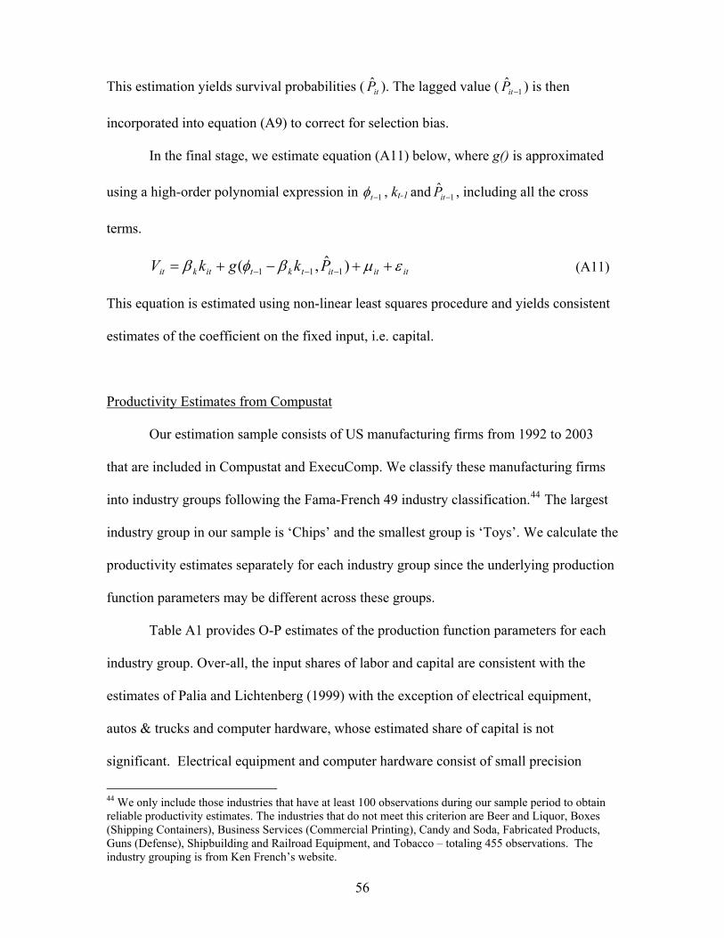
This estimation yields survival probabilities ( ). The lagged value ( ) is then

incorporated into equation (A9) to correct for selection bias.

itP̂ 1ˆ

itP

In the final stage, we estimate equation (A11) below, where g() is approximated

using a high-order polynomial expression in 1t , kt-1 and , including all the cross

terms.

1ˆ

itP

ititittktitkit PkgkV )ˆ,( 111 (A11)

This equation is estimated using non-linear least squares procedure and yields consistent

estimates of the coefficient on the fixed input, i.e. capital.

Productivity Estimates from Compustat

Our estimation sample consists of US manufacturing firms from 1992 to 2003

that are included in Compustat and ExecuComp. We classify these manufacturing firms

into industry groups following the Fama-French 49 industry classification.44 The largest

industry group in our sample is ‘Chips’ and the smallest group is ‘Toys’. We calculate the

productivity estimates separately for each industry group since the underlying production

function parameters may be different across these groups.

Table A1 provides O-P estimates of the production function parameters for each

industry group. Over-all, the input shares of labor and capital are consistent with the

estimates of Palia and Lichtenberg (1999) with the exception of electrical equipment,

autos & trucks and computer hardware, whose estimated share of capital is not

significant. Electrical equipment and computer hardware consist of small precision

44 We only include those industries that have at least 100 observations during our sample period to obtain reliable productivity estimates. The industries that do not meet this criterion are Beer and Liquor, Boxes (Shipping Containers), Business Services (Commercial Printing), Candy and Soda, Fabricated Products, Guns (Defense), Shipbuilding and Railroad Equipment, and Tobacco – totaling 455 observations. The industry grouping is from Ken French’s website.

56

57

instruments so it is quite plausible that only the share of labor is significant. The result

for autos and trucks, on the other hand, is surprising since we expect this to be a capital-

intensive industry. Hence, we drop the auto industry from our sample. Productivity

(TFP) is then calculated as the difference between actual and predicted output. As a

robustness check, we performed our analyses excluding the electrical equipment and

hardware industries; our findings are unchanged.

As an alternative to this two-factor production function, we also estimate a

production function with labor, capital and materials as inputs; our main findings are

unchanged. Moreover, the closest proxy available for material inputs is cost of goods

sold (Compustat data item 41). This is a noisy measure of materials since it includes

other items such as wages and rent. Thus, our preferred specification is that with only

labor and capital as inputs to production.

TABLE A1

PRODUCTION FUNCTION ESTIMATES BY INDUSTRY: OLLEY-PAKES (1996) METHODOLOGY Manufacturing Industries (SIC codes 2000-3999)

Factor Inputs Food Toys /

Recreation Books Consumer

Goods Clothing Medical

Equipment Drugs Chemicals Rubber &

Plastics Textiles Building

Materials 0.429*** 0.278*** 0.370*** 0.544*** 0.376*** 0.287*** 0.065** 0.266*** 0.314*** 0.191** 0.216*** Capital

(0.024) (0.056) (0.061) (0.044) (0.042) (0.052) (0.027) (0.010) (0.044) (0.077) (0.018)

0.399*** 0.689*** 0.419*** 0.165*** 0.398*** 0.708*** 1.152*** 0.482*** 0.778*** 0.713*** 0.745*** Labor (0.033) (0.085) (0.081) (0.059) (0.067) (0.060) (0.024) (0.024) (0.078) (0.093) (0.025)

Observations 444 154 256 389 292 506 801 605 110 188 484

Factor Inputs Steel Machinery Electrical Equipment

Autos & Trucks

Aircraft Petroleum & Gas

Computer Hardware

Electronic Equipment

Lab Equipment

Business Supplies

0.324*** 0.247*** 0.005 0.013 0.265** 0.362*** 0.058 0.079*** 0.144*** 0.210*** Capital (0.023) (0.031) (0.039) (0.031) (0.118) (0.028) (0.042) (0.018) (0.013) (0.010)

0.507*** 0.622*** 1.045*** 0.939*** 0.750*** 0.904*** 0.874*** 0.798*** 0.733*** 0.813*** Labor (0.041) (0.034) (0.040) (0.037) (0.148) (0.064) (0.048) (0.019) (0.018) (0.019)

Observations 508 799 249 445 103 182 302 1396 450 438

Notes: The production function is estimated separately by industry. Productivity is calculated as the residual between the predicted and actual output. We follow the Fama-French 49 industry classification taken from Ken French’s website. Data is from Compustat and ExecuComp for the period 1992-2003.

58

TABLE A2 PRODUCTIVITY INDEX VALUES BY INDUSTRY AND YEAR

Manufacturing Industries (SIC codes 2000-3999)

1993 1998 2003 Industry Mean Median Mean Median Mean Median

Food 0.03 0.05 0.21 0.23 0.29 0.22

Toys / Recreation 0.03 0.00 0.14 0.17 0.52 0.32

Books 0.06 0.04 0.12 0.09 0.12 0.05

Consumer Goods 0.07 0.04 0.34 0.29 0.54 0.63

Clothing -0.04 -0.13 0.17 0.17 0.34 0.14

Medical Equipment 0.00 -0.09 0.17 0.19 0.45 0.51

Drugs 0.06 0.04 0.29 0.19 0.28 0.29

Chemicals 0.01 0.00 0.06 0.09 0.17 0.12

Rubber & Plastics 0.01 0.01 0.32 0.40 0.30 0.29

Textiles 0.02 -0.02 0.17 0.12 0.24 0.20

Building Materials 0.05 0.07 0.17 0.21 0.29 0.31

Steel 0.09 0.14 0.39 0.38 0.44 0.43

Machinery 0.04 -0.02 0.29 0.32 0.30 0.27

Electrical Equipment 0.04 0.03 0.07 0.03 0.20 0.18

Aircraft -0.06 -0.09 0.28 0.24 0.24 0.18

Petroleum & Gas 0.04 -0.10 0.20 0.29 0.30 0.26

Computer Hardware 0.08 0.08 1.00 1.10 1.36 1.44

Electronic Equipment 0.15 0.18 0.54 0.49 0.83 0.86

Lab Equipment 0.06 0.05 0.33 0.29 0.35 0.31

Business Supplies 0.03 0.00 0.10 0.12 0.21 0.26

Full Sample

1992 1993 1994 1995 1996 1997

Mean 0.00 0.06 0.13 0.20 0.27 0.29

Median 0.00 0.05 0.12 0.17 0.24 0.26

1998 1999 2000 2001 2002 2003

Mean 0.31 0.35 0.43 0.40 0.38 0.43

Median 0.28 0.30 0.37 0.36 0.34 0.36Notes: The productivity index is constructed as follows: pindxit=prodv_estit – prodv_estj,1992, where prodv_estit is the productivity estimate for firm i in year t and prodv_estj,1992 is the mean productivity estimate for industry j in 1992. We follow the Fama-French 49 industry classification taken from Ken French’s website. Data is from Compustat and ExecuComp for the period 1992-2003.

59

Appendix B: Variable Construction All variables used as covariates are winsorized at the 1 % tails. (Compustat data item in parenthesis) B.1 Variables used in the Productivity Estimation Output = Sales (data12) deflated by the producer price index (PPI) at the four-digit SIC 45 Capital Stock = We use the perpetual inventory method to calculate the replacement value of the capital stock. The inputs are gross property plant and equipment (data7), depreciation (data14), capital expenditures (data128) and the price index for non-residential private fixed investment.46 See Salinger and Summers (1983) for more details. Labor = Employees (data29) Investment = Capital expenditures (data128) deflated by the price index for non-residential private fixed investment B.2 CEO Incentive Measures CEO cash compensation = salary + bonus CEO holdings = NS/total shares outstanding CEO delta = Equity delta + Option delta (or Equity delta if Option delta is missing)47

Equity delta = 01.0*PN S

Option delta = 01.0*/ueoption val1

PPON

jj

CEO vega = 01.0*/ueoption val1

ON

jj

NS and No are the number of shares and option grants, respectively, held by the CEO, P is the fiscal year end stock price reported by Execucomp, and if missing, we obtain it from Compustat. Option value is calculated using the Black-Scholes (1973) formula for European call options for every option grant j awarded to the CEO, accounting for dividends according to Merton (1973). We measure stock return volatility, σ, as the annualized standard deviation of monthly returns for the previous five years, reported by

45 The PPI is obtained from the Bureau of Labor and Statistics website. 46 This price index is obtained from the Bureau of Economic Analysis website. 47 There are 279 firm-year observations for which there is insufficient information to calculate the CEO’s option delta and vega.

60

ExecuComp, and if missing, is calculated using CRSP data.48 Hence (omitting the j subscript for notational simplicity): zNeP dT /ueoption val TPzNe dT '/ueoption val

Where d is the average dividend yield for the past three years (reported by Execucomp),

T is the time to maturity of the option, ,//ln 221 TdrTXPz X is the

exercise price while the risk free rate, r, is the yield on U.S. Treasuries with a corresponding time to maturity as the option grant. We follow Core and Guay’s (2002) methodology to estimate option values, which involves using information from the firm’s most recent proxy statement49 (available from Execucomp). For new option grants in a particular year, the exercise price and time to maturity are disclosed in the proxy statement. For options granted in previous years, we do the following: 1) We estimate the exercise price as the difference between the stock price and the average realizable value per option.50 2) The time to maturity of unexercisable option grants is the time to maturity of the most recent fiscal year’s grant minus one year while the time to maturity of exercisable option grants is the time to maturity of unexercisable option grants minus three years. If no new grants were made in the most recent fiscal year, the time to maturity for unexercisable and exercisable option grants are nine and six years, respectively. Finally, CEO delta and vega are calculated in 2003 dollars. B.3 Variables used as Determinants of Productivity Firm Size = Log(Total Assets) (data6) 51 Firm age = current year – incorporation year52 where available; if the incorporation year is unavailable, we use the earliest year on CRSP that a firm has a positive stock price or the earliest year in Compustat that a firm has non-missing data for total assets Industry Concentration Index = Herfindahl Index based on Compustat data. This is given by: Σαi

2 where αi is the output (sales) share of each firm in the industry in that particular

48 Our findings are unchanged if we use the standard deviation of daily returns for the previous 252 trading days. 49 They show that their proxies for delta and vega capture more than ninety-nine percent of the variation in these measures if constructed directly from the full information set (a ten year history of proxy statements). 50 Realizable value is the payoff realized by the CEO if the stock price is greater than the exercise price and the option is exercised. This is reported in Execucomp separately for exercisable and unexercisable options. 51 The use of total sales as a measure of firm size leaves our results mostly unchanged and qualitatively similar. We remain cautious however, with this alternative specification because total sales is the measure of output in the productivity estimation. 52 We are grateful to John Ritter for the use of his data on incorporation dates.

61

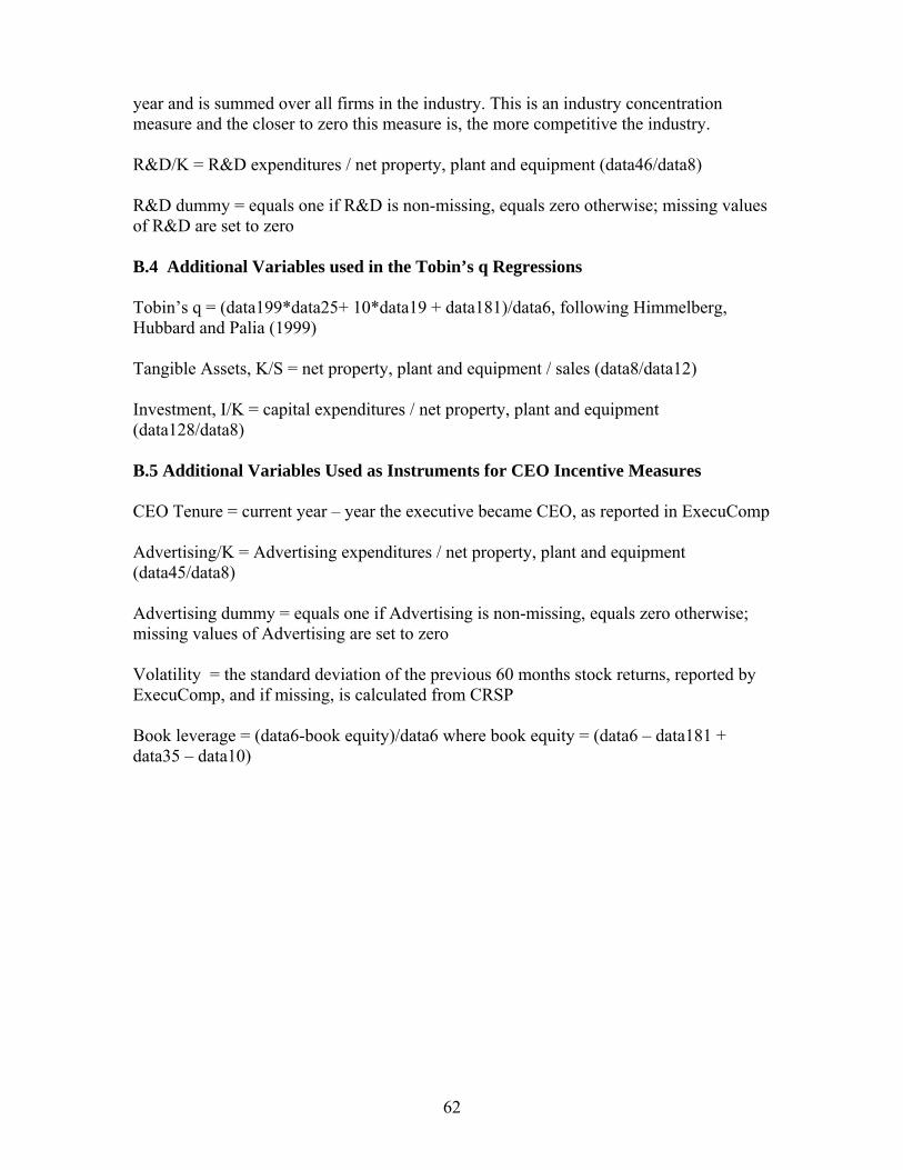
year and is summed over all firms in the industry. This is an industry concentration measure and the closer to zero this measure is, the more competitive the industry. R&D/K = R&D expenditures / net property, plant and equipment (data46/data8) R&D dummy = equals one if R&D is non-missing, equals zero otherwise; missing values of R&D are set to zero B.4 Additional Variables used in the Tobin’s q Regressions Tobin’s q = (data199*data25+ 10*data19 + data181)/data6, following Himmelberg, Hubbard and Palia (1999) Tangible Assets, K/S = net property, plant and equipment / sales (data8/data12) Investment, I/K = capital expenditures / net property, plant and equipment (data128/data8) B.5 Additional Variables Used as Instruments for CEO Incentive Measures CEO Tenure = current year – year the executive became CEO, as reported in ExecuComp Advertising/K = Advertising expenditures / net property, plant and equipment (data45/data8) Advertising dummy = equals one if Advertising is non-missing, equals zero otherwise; missing values of Advertising are set to zero Volatility = the standard deviation of the previous 60 months stock returns, reported by ExecuComp, and if missing, is calculated from CRSP Book leverage = (data6-book equity)/data6 where book equity = (data6 – data181 + data35 – data10)

62

Appendix C: Difference-GMM

Dynamic panel data estimators were originally developed by Holtz-Eakin, Newey

and Rosen (1988) and Arellano and Bond (1991), and are used to estimate first order

autoregressive models with individual specific effects (equation C1) using the

Generalized Method of Moments (GMM).

ititiit vyy 1, i=1,…N, t=2,…T, T>3 and || < 1 (C1)

In our model yit is the productivity variable. Our model includes potentially endogenous

right-hand-side variables such as CEO delta and vega, given by xit in equation C2.

itiittiit vxyy 1, i=1,…N, t=2,…T, T>3 and || < 1 (C2)

We take the first-difference of (C2) to remove unobserved time-invariant

individual specific effects, and then instrument the right-hand-side variables in the first-

differenced equations using levels of the series lagged two periods or more. This model

uses the standard assumption that the error terms are not auto-correlated and the set of

moment conditions in equations C3 and C4 hold,

itv

0, itsti vyE t=3,…T and 2s (C3)

0, itsti vxE t=3,…T and 2s (C4)

where is the first difference operator. If xit is pre-determined, then s≥1. Additional

moment conditions can be obtained by replacing xit with instruments zit where s≥1. (In

our model, CEO incentive variables are endogenous while variables used as instruments

are predetermined.) This methodology has two main advantages over other estimations

methods. First, estimates are not biased by any omitted variables that are constant over

time such as unobserved firm-specific effects. Second, the use of instrumental variables

allows one to consistently estimate the parameters of the model even in the presence of

63

endogenous variables. The validity of these instruments can be checked using the

standard Hansen J test of over-identifying restrictions. Arellano and Bond (1991) propose

an additional test, the m2 test, to verify that the assumption of no autocorrelation in the

error terms is satisfied.53 This latter test is important because the model follows a first

order autoregressive structure.

Appendix D: Instrument Set

Prior work has shown the following variables affect CEO compensation:

1) Firm size is related to agency costs since larger firms are more difficult to monitor.

Also, larger firms require highly skilled managers who demand greater compensation and

are thus wealthier. Thus larger firms would need higher levels of CEO incentives

(greater incentive-alignment or a steeper slope of the compensation contract). On the

other hand, rating agencies and top management may benefit from monitoring economies

of scale in larger firms. This would predict that larger firms require lower incentive

levels.

2) Firm age would affect CEO incentives for similar reasons as firm size, but would also

affect the composition of compensation packages. Younger firms are more likely to use

options and restricted stock grants.

3) CEO tenure is the number of years the executive has been the CEO of the company,

constructed from ExecuComp. CEO experience is a proxy for CEO wealth. To a certain

extent, it also captures the CEOs proximity to retirement. To avoid short horizon

53 This test is implemented by testing for the absence of second-order serial correlation in the first-differenced errors. The absence of second-order serial correlation in first-differences implies the absence of serial correlation in levels.

64

65

concerns, higher incentives levels would be necessary. Thus, higher tenures would be

related to higher incentive levels.

4) Stock return volatility is a proxy for CEO risk aversion. High stock return volatility

may distort the performance incentives of equity ownership in a firm due to the CEO’s

inability to diversify his portfolio. To mitigate this effect, CEOs of firms with high stock

return volatility are normally given more convex compensation contracts (e.g. stock

option grants) to induce more risk-taking behavior. Additionally, Guay (1999) shows

that stock return volatility is positively related to CEO vega.

5) R&D and advertising are measures of discretionary spending. Discretionary expenses

are more difficult to monitor and would thus require a higher level of incentives.

Additionally, Coles, Daniel and Naveen (2006) show that high R&D results in lower

CEO delta and higher CEO vega.

6) Finally, book leverage can control for agency costs according to Jensen’s (1986) free

cash flow theory. Higher leverage mitigates these agency costs and reduces the need for

high CEO incentive levels. Furthermore, Coles, Daniel and Naveen (2006) also show that

high leverage results in lower CEO delta and higher CEO vega.