A FAST PARALLEL ALGORITHM FOR SELECTED ...math.duke.edu/~jianfeng/paper/parallel.pdfA FAST PARALLEL...
27
A FAST PARALLEL ALGORITHM FOR SELECTED INVERSION OF STRUCTURED SPARSE MATRICES WITH APPLICATION TO 2D ELECTRONIC STRUCTURE CALCULATIONS LIN LIN * , CHAO YANG † , JIANFENG LU ‡ , LEXING YING § , AND WEINAN E ¶ Abstract. An efficient parallel algorithm is presented and tested for computing selected compo- nents of H -1 where H has the structure of a Hamiltonian matrix of two-dimensional lattice models with local interaction. Calculations of this type are useful for several applications, including elec- tronic structure analysis of materials in which the diagonal elements of the Green’s functions are needed. The algorithm proposed here is a direct method based on an LDL T factorization. The elimination tree is used to organize the parallel algorithm. Synchronization overhead is reduced by passing the data level by level along this tree using the technique of local buffers and relative indices. The performance of the proposed parallel algorithm is analyzed by examining its load balance and communication overhead, and is shown to exhibit an excellent weak scaling on a large-scale high performance parallel machine with distributed memory. Key words. selected inversion, parallel algorithm, electronic structure calculation AMS subject classifications. 65F05, 65F50, 65Z05 1. Introduction. In some scientific applications, we need to calculate a subset of the entries of the inverse of a given matrix. A particularly important example is in the electronic structure analysis using algorithms based on pole expansion [22, 24] where the diagonal and sometimes sub-diagonals of the discrete Green’s function or resolvent matrices are needed in order to compute the electron density. Other examples in which particular entries of the Green’s functions are needed can also be found in the perturbation analysis of impurities by solving Dyson’s equation in solid state physics [10], or the calculation of retarded and less-than Green’s function in electronic transport [6]. We will call this set of problems selected inversion of a matrix. From a computational viewpoint, it is natural to ask whether one can develop algorithms for selected inversion that is faster than inverting the whole matrix. This is possible at least in some cases. Consider, for example, the finite difference dis- cretization of a Hamiltonian operator of the form: H = - 1 2 Δ+ V (r). (1.1) Here Δ is the Laplacian operator, V is the external or effective potential. The resulting matrix has certain structure, as in lattice models in statistical or quantum mechanics with a local Hamiltonian. For such matrices, a fast but sequential algorithm has been proposed to extract the diagonal or sub-diagonal elements of its inverse matrix [23]. The algorithm is based on the LDL T factorization of H. The cost of the * Program in Applied and Computational Mathematics, Princeton University, Princeton, NJ 08544. Email: [email protected] † Computational Research Division, Lawrence Berkeley National Laboratory, Berkeley, CA 94720. Email: [email protected] ‡ Department of Mathematics, Courant Institute of Mathematical Sciences, 251 Mercer Street, New York, NY 10012. Email:[email protected] § Department of Mathematics and ICES, University of Texas at Austin, 1 University Sta- tion/C1200, Austin, TX 78712. Email: [email protected] ¶ Department of Mathematics and PACM, Princeton University, Princeton, NJ 08544. Email: [email protected] 1
Transcript of A FAST PARALLEL ALGORITHM FOR SELECTED ...math.duke.edu/~jianfeng/paper/parallel.pdfA FAST PARALLEL...

A FAST PARALLEL ALGORITHM FOR SELECTED INVERSION OFSTRUCTURED SPARSE MATRICES WITH APPLICATION TO 2D
ELECTRONIC STRUCTURE CALCULATIONS
LIN LIN ∗, CHAO YANG † , JIANFENG LU ‡ , LEXING YING § , AND WEINAN E ¶
Abstract. An efficient parallel algorithm is presented and tested for computing selected compo-nents of H−1 where H has the structure of a Hamiltonian matrix of two-dimensional lattice modelswith local interaction. Calculations of this type are useful for several applications, including elec-tronic structure analysis of materials in which the diagonal elements of the Green’s functions areneeded. The algorithm proposed here is a direct method based on an LDLT factorization. Theelimination tree is used to organize the parallel algorithm. Synchronization overhead is reduced bypassing the data level by level along this tree using the technique of local buffers and relative indices.The performance of the proposed parallel algorithm is analyzed by examining its load balance andcommunication overhead, and is shown to exhibit an excellent weak scaling on a large-scale highperformance parallel machine with distributed memory.
Key words. selected inversion, parallel algorithm, electronic structure calculation
AMS subject classifications. 65F05, 65F50, 65Z05
1. Introduction. In some scientific applications, we need to calculate a subsetof the entries of the inverse of a given matrix. A particularly important example isin the electronic structure analysis using algorithms based on pole expansion [22, 24]where the diagonal and sometimes sub-diagonals of the discrete Green’s functionor resolvent matrices are needed in order to compute the electron density. Otherexamples in which particular entries of the Green’s functions are needed can alsobe found in the perturbation analysis of impurities by solving Dyson’s equation insolid state physics [10], or the calculation of retarded and less-than Green’s functionin electronic transport [6]. We will call this set of problems selected inversion of amatrix.
From a computational viewpoint, it is natural to ask whether one can developalgorithms for selected inversion that is faster than inverting the whole matrix. Thisis possible at least in some cases. Consider, for example, the finite difference dis-cretization of a Hamiltonian operator of the form:
H = −12∆ + V (r). (1.1)
Here ∆ is the Laplacian operator, V is the external or effective potential. The resultingmatrix has certain structure, as in lattice models in statistical or quantum mechanicswith a local Hamiltonian. For such matrices, a fast but sequential algorithm hasbeen proposed to extract the diagonal or sub-diagonal elements of its inverse matrix[23]. The algorithm is based on the LDLT factorization of H. The cost of the
∗ Program in Applied and Computational Mathematics, Princeton University, Princeton, NJ08544. Email: [email protected]
†Computational Research Division, Lawrence Berkeley National Laboratory, Berkeley, CA 94720.Email: [email protected]
‡Department of Mathematics, Courant Institute of Mathematical Sciences, 251 Mercer Street,New York, NY 10012. Email:[email protected]
§Department of Mathematics and ICES, University of Texas at Austin, 1 University Sta-tion/C1200, Austin, TX 78712. Email: [email protected]
¶Department of Mathematics and PACM, Princeton University, Princeton, NJ 08544. Email:[email protected]
1

2 L. LIN, C. YANG, J. LU, L. YING AND W. E
fast algorithm is O(n1.5) for two dimensional (2D) problems and O(n2) for threedimensional problems, with n being the dimension of H. This is compared with acost of O(n3) for direct inversion of the full matrix.
The present paper follows the concept in [23], and focuses on the parallel imple-mentation of an LDLT factorization based selected inversion algorithm.
The paper is organized as follows. In section 2, we introduce briefly the mainconcept of selected inversion based on LDLT factorization. The algorithmic andimplementation details of a parallel procedure that we have developed for selected in-version is presented in section 3. The performance of such a procedure is demonstratedand analyzed in section 4. In particular, we show that our parallel implementationcan be used to solve problems defined on a 65, 535× 65, 535 grid with more than fourbillion degrees of freedom on 4,096 processors in less than 25 minutes. We present anapplication of the algorithm to an electronic structure calculation for a quantum dotand compare its performance with a standard approach implemented in the softwarepackage Octopus [4].
Standard linear algebra notations are used for vectors and matrices throughoutthe paper. We use Ai,j to denote the (i, j)-th element of A. When describing thealgorithms and their implementations, we often use letters in a typewriter font suchas A, L and D etc. to denote matrices stored in an appropriate format using anappropriate data structure. The letters I, J and K often serve the dual purposes ofbeing an integer index as well as representing a set that contains a number of integersas its members. Their meaning should be clear from the context. Occasionally, weuse a MATLAB [31] script to describe a simple algorithm. In particular, we use theMATLAB-style notation A(i:j,k:l) to denote a submatrix of A that consists of rowsi through j and columns k through l.
2. Selected Inversion Based on LDLT Factorization: The Basic Idea.There are two main steps in the LDLT factorization-based selected inversion algo-rithm. In the first step, we simply compute a sparse block LDLT factorization ofA. We assume here that A is nonsingular and all pivots produced in the LDLT
factorization are sufficiently large so that no row or column permutation is neededduring the factorization. In the second step, L and D are used to retrieve the selectedelements of A−1 with a computational complexity comparable to that of the sparseblock LDLT factorization. No additional storage is required in this step. The mainidea used here is very general. It dates back to [11], and is discussed in other recentwork [21, 23, 35]. Before we describe the algorithm, it will be helpful to first reviewthe major operations involved including the LDLT factorization. We will use densematrix for illustration first, and then discuss the case for sparse matrices.
2.1. An Algorithm for Computing the Inverse of a Dense Matrix. Let
A =(
α aT
a A
), (2.1)
with α 6= 0. The first step of an LDLT factorization produces a decomposition of Athat can be expressed by
A =(
1` I
) (α
A− aaT /α
) (1 `T
I
),
where ` = a/α and S = A − aaT /α is known as a Schur complement. The sametype of decomposition can be applied recursively to the Schur complement S until

FAST PARALLEL ALGORITHM FOR SELECTED INVERSION 3
its dimension becomes 1. The product of lower triangular matrices produced fromthe recursive procedure yields the final L factor. The (1, 1) entry of each Schurcomplement together with α become the diagonal entries of the D matrix.
The key observation made in [21] and [23] is that A−1 can be expressed by
A−1 =(
α−1 + `T S−1` −`T S−1
−S−1` S−1
). (2.2)
This expression suggests that once α and ` are known, the task of computing A−1
can be reduced to that of computing S−1.Because a sequence of Schur complements are produced recursively in the LDLT
factorization of A, the computation of A−1 can be organized in a recursive fashionalso. Clearly, the reciprocal of the last entry of D is the (n, n)-th entry of A−1.Starting from this entry, which is also the 1 × 1 Schur complement produced in the(n − 1)-th step of the LDLT factorization procedure, we can construct the inverseof the 2 × 2 Schur complement produced at the (n − 2)-th step of the factorizationprocedure, using the recipe given by (2.2). This 2×2 matrix is the trailing 2×2 blockof A−1. As we proceed from the lower right corner of L and D towards their upperleft corner, more and more elements of A−1 are recovered. The complete procedurecan be easily described by a MATLAB script shown in Algorithm 1.
Algorithm 1 A MATLAB script for computing the inverse of a dense matrix A givenits LDLT factorization.
Ainv(n,n) = 1/D(n,n);
for j = n-1:-1:1
Ainv(j+1:n,j) = -Ainv(j+1:n,j+1:n)*L(j+1:n,j);
Ainv(j,j+1:n) = Ainv(j+1:n,j)’;
Ainv(j,j) = 1/D(j,j) - L(j+1:n,j)’*Ainv(j+1:n,j);
end;
For clarity purpose, we use a separate array Ainv in Algorithm 1 to store thecomputed A−1. In practice, A−1 can be computed in place. That is, we can overwritethe array used to store L with the lower triangular part of A−1 incrementally.
2.2. Selected Inversion for Sparse Matrices. It is not difficult to observethat the complexity of Algorithm 1 is O(n3) because a matrix vector multiplicationinvolving a j × j dense matrix is performed at the jth iteration of this procedure,and n − 1 iterations are required to fully recover A−1. Therefore, when A is dense,this procedure does not offer any advantage over the standard way of computing A−1,which simply solves the matrix equation AX = I, where I is the n×n identity matrix.Furthermore, all elements of A−1 are needed and computed. No computation costcan be saved if we just want to extract selected elements (for example, the diagonalelements) of A−1.
However, when A is sparse, a tremendous amount of saving can be achieved if weare only interested in the diagonal of A−1. If the vector ` in (2.2) is sparse, computing`T S−1` does not require all elements of S−1 to be obtained in advance. Only thoseelements that appear in the rows and columns that correspond to the nonzero rowsof ` are required.
Therefore, to compute the diagonal of A−1, we can simply modify the procedureshown in Algorithm 1 so that at each iteration we only compute selected elementsof A−1 that will be needed by subsequent iterations of this procedure. It turns out

4 L. LIN, C. YANG, J. LU, L. YING AND W. E
that the elements that need to be computed is completely determined by the nonzerostructure of the lower triangular factor L. To be more specific, at the jth step of theselected inversion process, we compute A−1
i,j for all i such that Li,j 6= 0.To see why this type of selected inversion is sufficient, we only need to examine
the nonzero structure of the kth column of L for all k < j since such a nonzerostructure tells us which rows and columns of the trailing sub-block of A−1 are neededto complete the calculation of the (k, k)th entry of A−1. In particular, we would liketo find out which elements in the jth column of A−1 are required for computing A−1
i,k
for any k < j and i ≥ j.Clearly, when Lj,k = 0, the jth column of A−1 is not needed for computing the
kth column of A−1. Therefore, we only need to examine columns k of L such thatLj,k 6= 0. A perhaps not so obvious but critical observation is that for these columns,Li,k 6= 0 and Lj,k 6= 0 implies Li,j 6= 0 for all i > j. Hence computing the kth columnof A−1 will not require more matrix elements from the jth column of A−1 than thosethat have already been computed (in previous iterations,) i.e., elements A−1
i,j suchthat Li,j 6= 0 for i ≥ j.
These observations are well known in the sparse matrix factorization literature[9, 12]. They can be made more precise by using the notion of elimination tree [27].In such a tree, each node or vertex of the tree corresponds to a column (or row) of A.Assuming A can be factored as A = LDLT , a node p is the parent of a node j if andonly if
p = min{i > j|Li,j 6= 0}.
If Lj,k 6= 0 and k < j, then the node k is a descendant of j in the elimination tree.Such a tree can be used to clearly describe the dependency among different columnsin a sparse LDLT factorization of A. In particular, it is not too difficult to show thatconstructing the jth column of L requires contributions from all descendants of j thathave a nonzero matrix element in the jth row.
Similarly, we may also use the elimination tree to describe which selected elementswithin the trailing sub-block A−1 are required in order to obtain the (j, j)-th elementof A−1. In particular, it is not difficult to show that the selected elements must belongto rows and columns of A−1 that are among the ancestors of j.
2.3. A Block Algorithm. The selected inversion procedure described in Algo-rithm 1 and its sparse version can be modified to allow a block of rows and columnsto be modified simultaneously. A block algorithm can be described in terms a blockfactorization of A:
A =(
A11 BT21
B21 A22
)=
(I
L21 I
) (A11
A22 −B21A−111 BT
21
) (I LT
21
I
),
(2.3)where L21 = B21A
−111 and S = A22 − B21A
−111 BT
21 is the Schur complement. Inparticular, a block version of (2.2) can be expressed by
A−1 =(
A−111 + LT
21S−1L21 −LT
21S−1
−S−1L21 S−1
).
There are at least two advantages for a block algorithm:1. It allows us to use level 3 BLAS (Basic Linear Algebra Subroutine) to de-
velop an efficient implementation by exploiting memory hierarchy in modernmicroprocessors;
FAST PARALLEL ALGORITHM FOR SELECTED INVERSION 5
2. It reduces indirect addressing overhead in sparse matrix computation.If A is sparse, blocks can be defined in terms of what are called supernodes. A
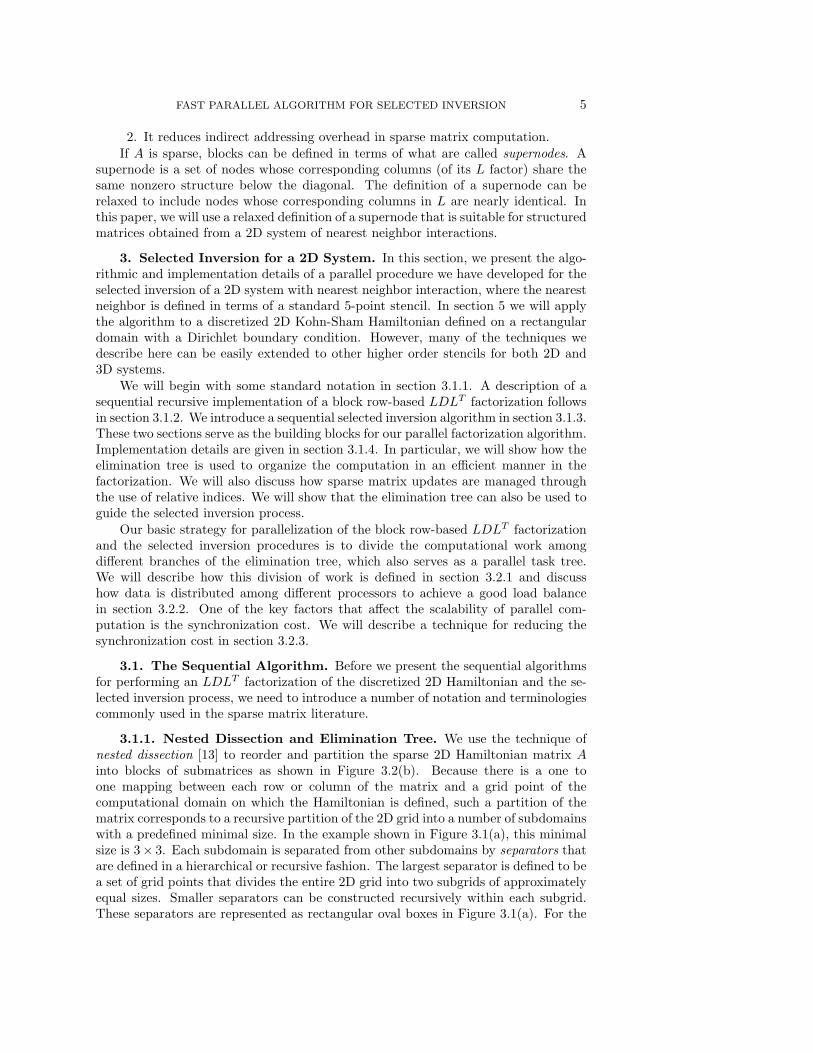
supernode is a set of nodes whose corresponding columns (of its L factor) share thesame nonzero structure below the diagonal. The definition of a supernode can berelaxed to include nodes whose corresponding columns in L are nearly identical. Inthis paper, we will use a relaxed definition of a supernode that is suitable for structuredmatrices obtained from a 2D system of nearest neighbor interactions.
3. Selected Inversion for a 2D System. In this section, we present the algo-rithmic and implementation details of a parallel procedure we have developed for theselected inversion of a 2D system with nearest neighbor interaction, where the nearestneighbor is defined in terms of a standard 5-point stencil. In section 5 we will applythe algorithm to a discretized 2D Kohn-Sham Hamiltonian defined on a rectangulardomain with a Dirichlet boundary condition. However, many of the techniques wedescribe here can be easily extended to other higher order stencils for both 2D and3D systems.
We will begin with some standard notation in section 3.1.1. A description of asequential recursive implementation of a block row-based LDLT factorization followsin section 3.1.2. We introduce a sequential selected inversion algorithm in section 3.1.3.These two sections serve as the building blocks for our parallel factorization algorithm.Implementation details are given in section 3.1.4. In particular, we will show how theelimination tree is used to organize the computation in an efficient manner in thefactorization. We will also discuss how sparse matrix updates are managed throughthe use of relative indices. We will show that the elimination tree can also be used toguide the selected inversion process.
Our basic strategy for parallelization of the block row-based LDLT factorizationand the selected inversion procedures is to divide the computational work amongdifferent branches of the elimination tree, which also serves as a parallel task tree.We will describe how this division of work is defined in section 3.2.1 and discusshow data is distributed among different processors to achieve a good load balancein section 3.2.2. One of the key factors that affect the scalability of parallel com-putation is the synchronization cost. We will describe a technique for reducing thesynchronization cost in section 3.2.3.
3.1. The Sequential Algorithm. Before we present the sequential algorithmsfor performing an LDLT factorization of the discretized 2D Hamiltonian and the se-lected inversion process, we need to introduce a number of notation and terminologiescommonly used in the sparse matrix literature.
3.1.1. Nested Dissection and Elimination Tree. We use the technique ofnested dissection [13] to reorder and partition the sparse 2D Hamiltonian matrix Ainto blocks of submatrices as shown in Figure 3.2(b). Because there is a one toone mapping between each row or column of the matrix and a grid point of thecomputational domain on which the Hamiltonian is defined, such a partition of thematrix corresponds to a recursive partition of the 2D grid into a number of subdomainswith a predefined minimal size. In the example shown in Figure 3.1(a), this minimalsize is 3× 3. Each subdomain is separated from other subdomains by separators thatare defined in a hierarchical or recursive fashion. The largest separator is defined to bea set of grid points that divides the entire 2D grid into two subgrids of approximatelyequal sizes. Smaller separators can be constructed recursively within each subgrid.These separators are represented as rectangular oval boxes in Figure 3.1(a). For the

6 L. LIN, C. YANG, J. LU, L. YING AND W. E
sake of convenience, we will call a set of row or column indices associated with eithera minimal subdomain or a separator a supernode. We will use uppercase typewritertypeface letters such as I to denote such a supernode. We should note that thisdefinition of supernode is different from the conventional definition used in the sparsematrix literature [34], where the columns of L corresponding to a supernode arerequired to take exactly the same sparsity pattern below the diagonal. Our definitionis more relaxed to include nodes whose corresponding columns of L are nearly identicalin order to take full advantage of BLAS3. If the supernodes are numbered in a way asshown in Figure 3.1(b), the corresponding matrix exhibits a sparsity pattern shownin Figure 3.2(b).
The hierarchical relationship among different separators can be organized in a treestructure shown in Figure 3.2(a). The largest separator (supernode 31) that dividesthe entire grid in half forms the root of the tree. The separators that divide eachsubgrid produced from the first division are the children of the root. The minimalsubdomains that are connected by the lowest-level separators form the leaves of thetree. It turns out that this separator tree is identical to the elimination tree associatedwith the block LDLT factorization of the reordered and portioned matrix A shownin Figure 3.2(b). Each node of the tree corresponds to a supernode. The orderingof supernodes follows a postorder traversal of the tree, i.e., a node is traversed onlyafter all its children have been traversed.
(a) Nested dissection partitionand separators
3
1
2
4
5
67
8
9
10
11
13
12
14
3115
16
17
18
19
20
2122
23 26
27
2829
30
24
25
(b) The ordering of the supern-odes.
Fig. 3.1. The nested dissection of a 15× 15 grid and the ordering of the supernodes associatedwith this partition.
3.1.2. Block LDLT Factorization. There are a number of ways to implementthe block LDLT factorization (2.3) of a sparse matrix A. They differ by the order inwhich the rows and columns of a Schur complement are updated. The review papers[17,33,34,37] contain thorough discussions on the left-looking, right-looking and mul-tifrontal algorithms in which Schur complements are updated column by column. Thefactorization phase in the recently developed hierarchical Schur complement algorithm[23] can be regarded as an efficient right-looking implementation on a 2D rectangulargrid. The LDLT factorization we choose to implement follows a row-based approachpresented in [7]. This approach is also known as the bordering algorithm in [28,34]. Ifwe ignore the sparsity structure of A and L for the moment and assume that A and Lhave been partitioned into nblocks block rows and columns indexed by J, a block row-based factorization algorithm can be succinctly described by the pseudocode shownin Algorithm 2. Note that in the pseudocode, the L matrix is constructed one blockrow at a time by solving a set of triangular systems (steps 1 and 2 of the algorithm)

FAST PARALLEL ALGORITHM FOR SELECTED INVERSION 7
31
15
7
3
1 2
6
4 5
14
10
8 9
13
11 12
30
22
18
16 17
21
19 20
29
25
23 24
28
26 27
(a) The separator (or elimination) tree inpostorder
(b) The reordered and partitioned matrixA
Fig. 3.2. The separator tree associated with the nested dissection of the 15 × 15 grid shownin Figure 3.1(a) can also be viewed as the supernode elimination tree associated with the LDLT
factorization of the 2D Laplacian defined on that grid.
at each iteration. The index J should be interpreted as both a block row or columnindex and a set of rows and columns within the block indexed by J. This dual-purposenotation will be used throughout this paper.
Algorithm 2 A row-based LDLT factorization of a symmetric matrix A.for J = 1 to nblocks do
Solve Y*L(1:J-1,1:J-1)T = A(J,1:J-1) for Y;Solve L(J,1:J-1)*D(1:J-1,1:J-1) = Y for L(J,1:J-1);L(J,J) ← identity matrix;D(J,J) ← A(J,J) - L(J,1:J-1)*YT ;
end for
When A is sparse, we should exploit the sparsity structure of L in order to mini-mize the number of operations. It is well known in the sparse matrix literature that,at each iteration J, the sparsity pattern of Y and L(J,1:J-1) is completely deter-mined by the nonzero structure of the descendants of node J in the elimination tree.To be specific, Y(I) (or L(I,J)) is nonzero if and only if node I is a descendent ofJ in the elimination tree. Furthermore, the way in which Y(I) is computed can beexpressed in terms of a traversal of the sub-tree rooted at I [27]. As a result, step 1of the factorization procedure given in Algorithm 2 can be carried out efficiently byfollowing the pseudocode given in Algorithm 3.
Algorithm 3 A triangular solve algorithm guided by an elimination tree.Y ← A(1:J-1,J);for I ∈ {Descendants of J} do
for K ∈ {Descendants of I} doY(I)← Y(I)− L(I, K) ∗ Y(K);
end forend for
As we can see from Algorithm 3, Y(I) can be computed only if Y(K) have beencalculated for all K that are descendants of I. Hence, to compute Y(I), the descendants
8 L. LIN, C. YANG, J. LU, L. YING AND W. E
of node I must be traversed in a proper order. The postorder [5] of the nodes in theelimination tree shown in Figure 3.2(a) satisfies this ordering requirement. Moreover,such an order allows us to implement the pseudocode in Algorithm 3 in a recursivefashion, as we will show in section 3.1.4.
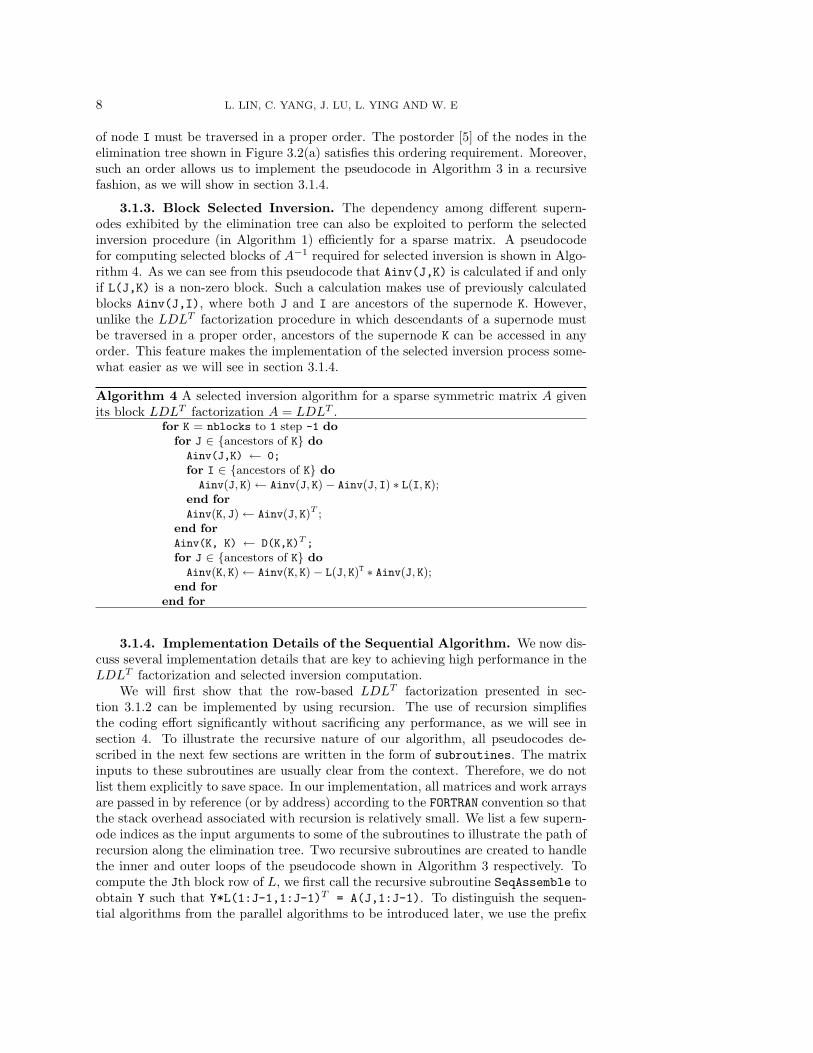
3.1.3. Block Selected Inversion. The dependency among different supern-odes exhibited by the elimination tree can also be exploited to perform the selectedinversion procedure (in Algorithm 1) efficiently for a sparse matrix. A pseudocodefor computing selected blocks of A−1 required for selected inversion is shown in Algo-rithm 4. As we can see from this pseudocode that Ainv(J,K) is calculated if and onlyif L(J,K) is a non-zero block. Such a calculation makes use of previously calculatedblocks Ainv(J,I), where both J and I are ancestors of the supernode K. However,unlike the LDLT factorization procedure in which descendants of a supernode mustbe traversed in a proper order, ancestors of the supernode K can be accessed in anyorder. This feature makes the implementation of the selected inversion process some-what easier as we will see in section 3.1.4.
Algorithm 4 A selected inversion algorithm for a sparse symmetric matrix A givenits block LDLT factorization A = LDLT .
for K = nblocks to 1 step -1 dofor J ∈ {ancestors of K} doAinv(J,K) ← 0;
for I ∈ {ancestors of K} doAinv(J, K)← Ainv(J, K)− Ainv(J, I) ∗ L(I, K);
end forAinv(K, J)← Ainv(J, K)T ;
end forAinv(K, K) ← D(K,K)T ;
for J ∈ {ancestors of K} doAinv(K, K)← Ainv(K, K)− L(J, K)T ∗ Ainv(J, K);
end forend for
3.1.4. Implementation Details of the Sequential Algorithm. We now dis-cuss several implementation details that are key to achieving high performance in theLDLT factorization and selected inversion computation.
We will first show that the row-based LDLT factorization presented in sec-tion 3.1.2 can be implemented by using recursion. The use of recursion simplifiesthe coding effort significantly without sacrificing any performance, as we will see insection 4. To illustrate the recursive nature of our algorithm, all pseudocodes de-scribed in the next few sections are written in the form of subroutines. The matrixinputs to these subroutines are usually clear from the context. Therefore, we do notlist them explicitly to save space. In our implementation, all matrices and work arraysare passed in by reference (or by address) according to the FORTRAN convention so thatthe stack overhead associated with recursion is relatively small. We list a few supern-ode indices as the input arguments to some of the subroutines to illustrate the path ofrecursion along the elimination tree. Two recursive subroutines are created to handlethe inner and outer loops of the pseudocode shown in Algorithm 3 respectively. Tocompute the Jth block row of L, we first call the recursive subroutine SeqAssemble toobtain Y such that Y*L(1:J-1,1:J-1)T = A(J,1:J-1). To distinguish the sequen-tial algorithms from the parallel algorithms to be introduced later, we use the prefix

FAST PARALLEL ALGORITHM FOR SELECTED INVERSION 9
Seq in subroutine names associated with the sequential algorithms and the prefix Parin those that are associated with the parallel algorithms. Algorithm 5 shows howSeqAssemble is used in the main LDLT factorization program that computes oneblock row of L and D at a time.
Algorithm 5 The major steps of a recursive implementation of the block row-basedLDLT factorization algorithm for a symmetric matrix A.
subroutine SeqBlockLDLT
for J = 1 to nblocks doY ← A(J,1:J-1);
Update Y by calling SeqAssemble(J,J);
D(J,J) ← Y(J);
Update L(J,1:J) and D(J,J) by calling SeqInv(J);
end forreturn L, D;end subroutine
The pseudocode given in the left column of Algorithm 6 shows that, at the Jthiteration, the SeqAssemble subroutine traverses down the subtree rooted at J inpostorder until the first argument I becomes a leaf node at which Y(I) is simplyA(I,J). Once all descendants of the node I have been traversed, indicating that Y(K)is available for all descendants K of I, we use a second subroutine SeqSum (shown inthe right column of Algorithm 6) to perform the summation required in the inner loopof the triangular solve shown in Algorithm 3. For each descendent I of J, the SeqSumsubroutine traverses the subtree rooted at I again to collect the matrices Y(K) thathave already been computed. It accumulates the product of Y(K) and L(I,K) in ahierarchical fashion in a workspace denoted by Buffer in Algorithm 6. The reasonwhy we use a workspace to accumulate all contributions from the descendants of Iinstead of applying updates to Y(I) directly will become clear later in this section.
Algorithm 6 Recursive implementation of the triangular solve shown in Algorithm 3.subroutine SeqAssemble(I,J)
if (I is a leaf node) return;for K = {children of I} do
Update Y by calling SeqAssemble(K,J)
recursively;end forBuffer = 0;
Update Buffer by callingSeqSum(Buffer,I,I,J);
Y(I)← Y(I)− transpose(Buffer);return Y;end subroutine
subroutine SeqInv(J)
D(J, J)← D(J, J)−1;for I ∈ {descendants of J} doL(J,I) ← Y(I)*D(J,J);
end forreturn L, D;end subroutine
subroutine SeqSum(Buffer,K,I,J)
if (K is not a leaf node) thenfor C = {children of K} do[RelI,RelJ] =
GetRelIndex(C,K,I,J);
Update part of Buffer by callingSeqSum(Buffer(RelI,RelJ),C,I,J)
recursively;end for
end ifif ( K 6= I ) thenBuffer = Buffer + L(I, K)⊗ Y(K);
end ifreturn Buffer;end subroutine

10 L. LIN, C. YANG, J. LU, L. YING AND W. E
To complete the computation of the Jth block row of L and D, we need to invertthe diagonal block D(J,J), and multiply D(J, J)−1 with Y(I) for all descendants I ofJ as shown in the SeqInv subroutine in Algorithm 6.
Up to this point, we have treated the matrix blocks L(J,I) as if they are densematrices. For the 2D Hamiltonian we consider in this paper, a large number of the off-diagonal matrix blocks in L are quite sparse. For example, in Figure 3.3, which showsthe sparsity pattern of the L factor associated with a 2D Hamiltonian defined on a 7×7grid as well as the block structure obtained from a 2-level nested dissection reordering,the L(7,1) block is 7×9, but contains only 6 nonzero entries at its upper right corner.In order to carry out the summation process in the SeqSum subroutine efficiently, wemust take advantage of these sparsity structures, which can be predetermined by asymbolic analysis procedure described in [25]. In particular, we should not store thezero rows and columns in L(I,K) and Y(K), and we should exclude these rows andcolumns when these two matrices are multiplied. As a result, the product of thenonzero rows and columns of these matrices will have a smaller dimension, and itneeds to be placed at a proper location in the destination workspace. We will callthe multiplication of the nonzero rows and columns of L(I,K) and Y(K) a restrictedmatrix-matrix multiplication, and denote it by ⊗.
To implement such a restricted matrix-matrix multiplication, we need to keeptrack of the size and the starting location of nonzero rows and columns of L(J,I) forall J and I. To reduce the bookkeeping overhead, we treat some of the zero entries inL(J,I) as nonzeros and store them explicitly. For example, in Figure 3.3, the nonzeroentries appear within the 3 × 3 submatrix at the upper right corner of the L(7,1)block. Even though the lower triangular part of this 3 × 3 submatrix is completelyzero, we store the entire submatrix and record its starting location within L(7,1).
Fig. 3.3. Sparsity pattern of the L factor associated with a Hamiltonian discretized on a 7× 7grid.
Once the positions and sizes of the non-zero submatrices within L(I,K) and Y(K)are known, the size of the product of these submatrices and its location within Y(I)can be determined for all ancestors I of K. For example, it is easy to see from Figure 3.3that the product of the nonzero submatrices of L(7,1) and Y(1) is a 3 × 3 matrix,and it should be accumulated at the upper left corner of Y(1) with the starting rowand column positions of (1, 1). We call such type of row and column position indicesabsolute indices. Using these absolute indices, we can in fact perform the summationin the inner loop of Algorithm 3 by adding the product of the nonzero submatrices ofL(I,K) and Y(K) directly to the destination location in Y(I). However, such a strategy

FAST PARALLEL ALGORITHM FOR SELECTED INVERSION 11
creates a synchronization bottleneck in the parallel LDLT factorization algorithm tobe discussed in section 3.2. To overcome this problem, we developed a hierarchicalscheme for accumulating the product of L(I,K) and Y(K) as the descendants of nodeI are traversed by the SeqSum subroutine in Algorithm 6. We sketch the basic ideasof this scheme here and will explain how it helps to eliminate the synchronizationbottleneck in a parallel LDLT factorization in the next section.
As illustrated in Algorithm 6, a work array Buffer, which has the same size asthe number of nonzero rows and columns in Y(I), is created when node I is traversedby the SeqAssemble subroutine. This array is used to accumulate all L(I,K)*Y(K)contributions from the descendants of I. Because the multiplication of the nonzerosubmatrices of L(I,K) and Y(K) often produces a matrix with a much smaller dimen-sion (than that of the Buffer array), a subblock of Buffer is passed down from aparent to its children recursively as the descendants of I are traversed by the SeqSumsubroutine. The reason that it is sufficient to pass a subblock of the Buffer arrayfrom a parent to its children (instead of passing a subblock of Buffer directly fromnode I to its descendants) is that the set of nonzero rows and columns associatedwith L(I,R)*Y(R) is a subset of the nonzero rows and columns that are associatedwith L(I,K)*Y(K) if R is a child of K. Hence, when the product of the nonzero rowsand columns of L(I,R) and Y(R) is accumulated in the Buffer array, we only need toknow the relative position of this product in the subblock of the Buffer array ownedby its parent K. The row and column indices that define such a position are calledrelative indices. The use of relative indices is not new. Similar ideas date back to [39],and they are also used in both left-looking and multifrontal algorithms [8, 29,34].
Restricted matrix-matrix multiplication must also be used to achieve high perfor-mance in the selected inversion process. During the calculation of Ainv(J,K), selectedrows and columns of Ainv(J,I) must be extracted before the submatrix associatedwith these rows and columns can be multiplied with the corresponding nonzero rowsand columns of L(I,K). These rows and columns are placed in a Buffer array inAlgorithm 7. The Buffer array is then multiplied with the corresponding nonzerocolumns of L(I,K). However, because the ancestors of the node K in Algorithm 4do not have to be visited in a hierarchical order, the use of relative indices is notnecessary. Absolute indices, which are obtained by the GetAbsIndex function in Al-gorithm 7, can be used to retrieve the desire submatrix block from Ainv(J,I) in asequential algorithm. This kind of restricted retrieval of Ainv(J,I) will become morecomplicated when the selected inversion of A is carried out in parallel. In that case,both absolute and relative indices need to be used.
It should be noted that we use A, L, D, Ainv and Y as separate variables inAlgorithms 5 and 7 only for clarity. In our implementation, A, L, D and Y share thesame storage space allocated in advance. Moreover, L is incrementally overwrittenby Ainv. Therefore, the memory requirement of our implementation is roughly whatis needed to store L in a block compressed column format plus a few extra arrays oflimited size that are used as workspace (such as Buffer).
3.2. Parallelization. The sequential algorithm described above is very efficientfor problems that can be stored on a single processor. For example, we have used thealgorithm to compute the diagonal of a discretized Kohn-Sham Hamiltonian definedon a 2047 × 2047 grid. The entire computation, which involves more than 4 milliondegrees, took less than 2 minutes on an AMD Opteron processor.
For larger problems that we would like to solve in electronic structure calculation,the limited amount of memory on a single processor makes it difficult to store the L

12 L. LIN, C. YANG, J. LU, L. YING AND W. E
Algorithm 7 Selected inversion of A with restricted matrix-matrix multiplicationgiven its block LDLT factorization.
subroutine SeqSelInverse
for K = nblocks to 1 step -1 dofor J ∈ {ancestors of K} doAinv(J,K) ← 0;
for I ∈ {ancestors of K} do[IA,JA] ← GetAbsIndex(L,K,I,J);
Buffer ← selected rows and columns of Ainv(J,I) starting at (IA, JA)
Ainv(J, K)← Ainv(J, K)− Buffer⊗ L(I, K);end forAinv(K,J) ← transpose(Ainv(J,K));
end forAinv(K,K) ← D(K, K)−1;for J ∈ {ancestors of K} doAinv(K, K)← Ainv(K, K)− L(J, K)T ⊗ Ainv(J, K);
end forend forreturn Ainv;end subroutine
and D factors in-core. Furthermore, because the complexity of the computation isO(n3/2) [23], the CPU time required to complete a calculation on a single processorwill eventually become excessively long.
Thus, it is desirable to modify the sequential algorithm so that the LDLT fac-torization and selected inversion process can be performed in parallel on multipleprocessors. The parallel algorithm we describe below focuses on distributed memorymachines that do not share a common pool of memory.
3.2.1. Task Parallelism. The elimination tree associated with the LDLT fac-torization of the reordered A (using nested dissection) provides natural guidance forparallelizing the factorization calculation. It can thus be viewed also as a paralleltask tree. We divide the computational work among different branches of the tree. Abranch of the tree is defined to be a path from the root to a node K at a given level` as well as the entire subtree rooted at K. The choice of ` depends on the numberof processors available. Our parallel algorithm requires the number of processors p tobe a power of two, and ` is set to log2(p) + 1.
In terms of tree node to processor mapping, each node at level ` or below isassigned to a unique processor. Above level `, each node is shared by multiple pro-cessors. The amount of sharing is hierarchical, and depends on the level at whichthe node resides. To be specific, a level-k node is shared by 2`−k processors. We willuse procmap(J) in the following discussion to denote the set of processors assigned tonode J. Each processor is labeled by an integer processor identification (id) numberbetween 0 and p− 1. This processor id is known to each processor as mypid.
Because each processor works on a particular branch of the tree, the recursiveprocedure shown in Algorithm 6 must be modified so that the SeqAssemble andSeqSum subroutines do not traverse the entire tree on each processor. In terms ofparallelism, it will be convenient to think of the subtree rooted at a level-` node asan aggregated leaf node. Figure 3.4(a) shows how different nodes in an eliminationtree are mapped to four processors used in a parallel calculation. The subtree rooted

FAST PARALLEL ALGORITHM FOR SELECTED INVERSION 13
31
15
7
3
1 2
6
4 5
14
10
8 9
13
11 12
30
22
18
16 17
21
19 20
29
25
23 24
28
26 27
(a) Parallel task tree (b) Columns of the L factor are parti-tioned and distributed among differentprocessors.
Fig. 3.4. Task parallelism expressed in terms of parallel task tree and correponding matrix toprocessor mapping.
at the 3rd level nodes are enclosed by dashed line boxes to indicate that they areaggregated leaf nodes of the parallel task tree which is enclosed by the solid line box.
The main structures of the parallel block LDLT factorization and selected in-version procedures are shown in Algorithm 8. Both parallel procedures make use ofthe sequential algorithms presented earlier to perform necessary calculations that arelimited to an aggregated leaf node. In the case of LDLT factorization, each processorfirst uses Algorithm 5 to factor a diagonal block of A associated with an aggregateleaf node J. This computation is completely independent from similar calculationsperformed simultaneously by other processors. As each processor moves from an ag-gregated leaf node towards the root, which is indicated by the while loop in the leftcolumn of Algorithm 8, it uses the subroutine ParAssemble (which is the parallelanalog to SeqAssemble) to solve Y*L(1:J-1,1:J-1)=A(J,1:J-1) for Y in parallel.As we can see from the left column of Algorithm 9, the execution of ParAssemble byeach processor is recursive also. Each processor simply uses mypid and procmap toselect an appropriate branch to move down the parallel task tree. For each node Ialong that branch, processors that belong to procmap(I) all contribute to the parallelcomputation of Y(I), which requires communications among these processors. Even-tually, each processor will reach a leaf node I. When that happens, ParAssemble willcall SeqAssemble to traverse into the subtree rooted at I in postorder to computeY(K) for all K that are descendants of I, just like how it is done in the sequentialalgorithm. No inter-processor communication is needed in SeqAssemble.
Once all descendants of I along a particular branch of the parallel task tree havebeen traversed, including those that are within an aggregated leaf node, we use a newsubroutine ParSum in Algorithm 9 to add up the L(I,K)*Y(K) contributions from alldescendants K of I. The ParSum subroutine also moves down a branch of the paralleltask tree on each processor until it reaches an aggregated leaf node where the SeqSumsubroutine is called to sum up L(I,K)*Y(K) for all K that are in the aggregated leaf.As the ParSum recursion backtracks towards node I, it merges contributions fromdifferent branches of the parallel task tree in a hierarchical fashion. Communicationis required in the merging process which must be implemented with care to minimizingthe synchronization cost. We will discuss the implementation detail in section 3.2.3.
14 L. LIN, C. YANG, J. LU, L. YING AND W. E
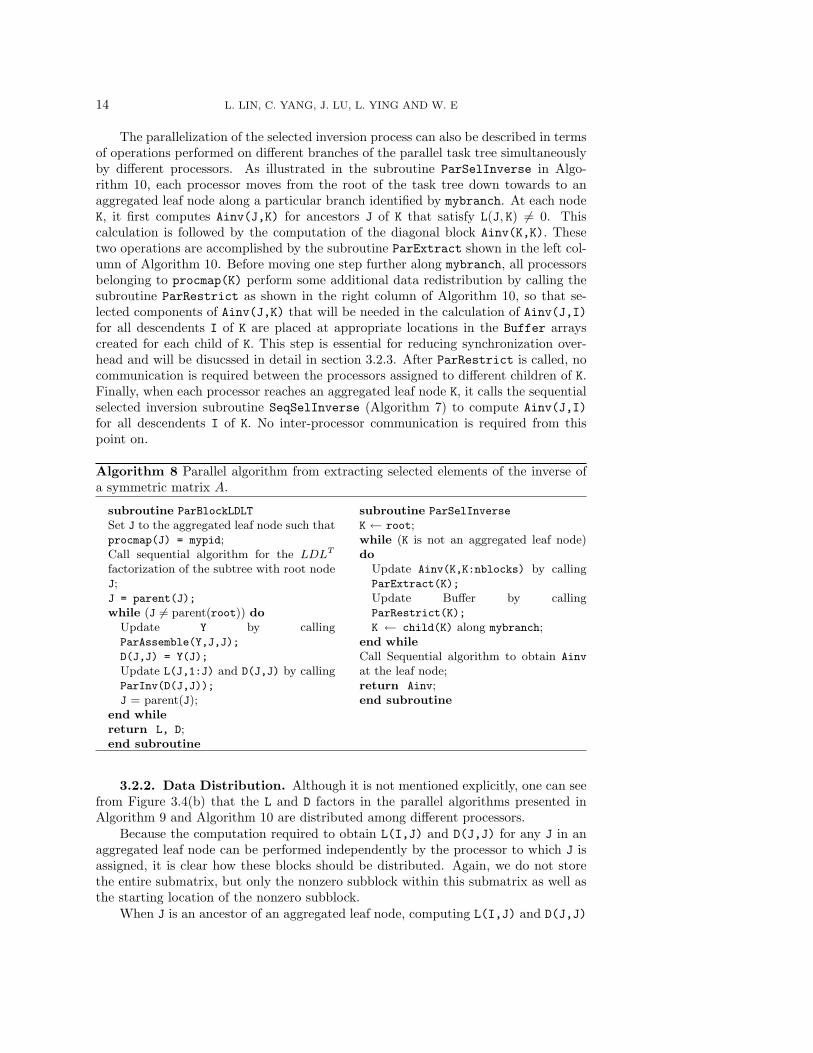
The parallelization of the selected inversion process can also be described in termsof operations performed on different branches of the parallel task tree simultaneouslyby different processors. As illustrated in the subroutine ParSelInverse in Algo-rithm 10, each processor moves from the root of the task tree down towards to anaggregated leaf node along a particular branch identified by mybranch. At each nodeK, it first computes Ainv(J,K) for ancestors J of K that satisfy L(J, K) 6= 0. Thiscalculation is followed by the computation of the diagonal block Ainv(K,K). Thesetwo operations are accomplished by the subroutine ParExtract shown in the left col-umn of Algorithm 10. Before moving one step further along mybranch, all processorsbelonging to procmap(K) perform some additional data redistribution by calling thesubroutine ParRestrict as shown in the right column of Algorithm 10, so that se-lected components of Ainv(J,K) that will be needed in the calculation of Ainv(J,I)for all descendents I of K are placed at appropriate locations in the Buffer arrayscreated for each child of K. This step is essential for reducing synchronization over-head and will be disucssed in detail in section 3.2.3. After ParRestrict is called, nocommunication is required between the processors assigned to different children of K.Finally, when each processor reaches an aggregated leaf node K, it calls the sequentialselected inversion subroutine SeqSelInverse (Algorithm 7) to compute Ainv(J,I)for all descendents I of K. No inter-processor communication is required from thispoint on.
Algorithm 8 Parallel algorithm from extracting selected elements of the inverse ofa symmetric matrix A.
subroutine ParBlockLDLT
Set J to the aggregated leaf node such thatprocmap(J) = mypid;Call sequential algorithm for the LDLT
factorization of the subtree with root nodeJ;J = parent(J);
while (J 6= parent(root)) doUpdate Y by callingParAssemble(Y,J,J);
D(J,J) = Y(J);
Update L(J,1:J) and D(J,J) by callingParInv(D(J,J));
J = parent(J);end whilereturn L, D;end subroutine
subroutine ParSelInverse
K ← root;while (K is not an aggregated leaf node)do
Update Ainv(K,K:nblocks) by callingParExtract(K);
Update Buffer by callingParRestrict(K);
K ← child(K) along mybranch;end whileCall Sequential algorithm to obtain Ainv
at the leaf node;return Ainv;end subroutine
3.2.2. Data Distribution. Although it is not mentioned explicitly, one can seefrom Figure 3.4(b) that the L and D factors in the parallel algorithms presented inAlgorithm 9 and Algorithm 10 are distributed among different processors.
Because the computation required to obtain L(I,J) and D(J,J) for any J in anaggregated leaf node can be performed independently by the processor to which J isassigned, it is clear how these blocks should be distributed. Again, we do not storethe entire submatrix, but only the nonzero subblock within this submatrix as well asthe starting location of the nonzero subblock.
When J is an ancestor of an aggregated leaf node, computing L(I,J) and D(J,J)

FAST PARALLEL ALGORITHM FOR SELECTED INVERSION 15
Algorithm 9 Parallel recursive implementation of the triangular solve shown in Al-gorithm 3.
subroutine ParAssemble(I,J)
if (mypid ∈ procmap(I)) thenif (I is not an aggregated leaf node)then
for K ∈ {children of I} doUpdate Y in parallel by callingParAssemble(K,J) recursively;
end forUpdate Buffer in parallel by call-ing ParSum(Buffer,I,I,J);
elseUpdate Y by callingSeqAssemble(I, J);Update Buffer by callingSeqSum(Buffer,I,I,J);
end ifY(I) ← Y(I) -
transpose(Buffer);
end ifreturn Y;end subroutine
subroutine ParInv(J)
D(J, J)← D(J, J)−1;for I ∈ {Descendants of J} doL(J,I) ← Y(I) * D(J,J);
end forreturn L, D;end subroutine
subroutine ParSum(Buffer,K,I,J)
if (mypid ∈ procmap(K)) thenif (K is not an aggregated leaf node) then
allocate CBuffer{C} for each child C of K;for C ∈ {children of K} do
Update CBuffer{C} by callingParSum(CBuffer{C},C,I,J) recur-sively.
end forfor C ∈ {Children of K} do[IR,JR] ← GetRelIndex(C,K,I,J);
Merge CBuffer{C} into Buffer(IR,JR)
using PDGEMR2D;end for
elsefor C ∈ {children of K} do[IR,JR] ← GetRelIndex(C,K,I,J);
Update sequential part of Buffer bycalling SeqSum(Buffer(IR,JR),C,I,J)
recursively;end for
end ifif (K 6= I) thenBuffer = Buffer + L(I, K) ⊗ Y(K);
end ifend ifreturn Buffer;end subroutine
Algorithm 10 Parallel implementation of selected inversion of A given its blockLDLT factorization.
subroutine ParExtract(K)
for J ∈ {ancestors of K} doAinv(J,K) ← 0;
for I ∈ {ancestors of K} do
Ainv(J, K) ← Ainv(J, K) −Buffer(J, I)⊗ L(I, K);
end for
Ainv(K,J) ← Ainv(J,K)T ;
end forAinv(K,K) ← D(K,K);
for J ∈ {ancestors of K} doAinv(K, K) ∈ Ainv(K, K)− L(J, K)T ⊗Ainv(J, K);
end forreturn Ainv;end subroutine
subroutine ParRestrict(K)
if (K is the root) thenBuffer ← D(K,K);
end iffor C ∈ {children of K} do
for all I,J ∈ {ancestors of K} doif L(J, C) 6= 0 and L(I, C) 6= 0) then[IR,JR] ∈GetRelIndex(C,K,I,J);
Restrict Buffer(J,I) to a subma-trix starting at (IR, JR).
end ifend for
end forreturn Buffer;end subroutine

16 L. LIN, C. YANG, J. LU, L. YING AND W. E
requires the participation of all processors that are assigned to to this node, i.e.,procmap(J). As a result, it is natural to divide the nonzero subblock in L(I,J) andD(J,J) into smaller submatrices, and distribute them among all processors that belongto procmap(J). Distributing these smaller submatrices among different processors isalso necessary for overcoming the memory limitation imposed by a single processor.For example, for a 2D Hamiltonian defined on a 16, 383×16, 383 grid, the dimension ofD(J,J) is 16, 383 for the root node J. This matrix is completely dense, hence contains16, 3832 matrix elements. If each element is stored in double precision, the totalamount of memory required to store D(J,J) alone is roughly 2.1 gigabytes (GB). Aswe will see in section 4, the distribution scheme we use in our parallel algorithm leadsto only a mild increase of memory usage per processor as we increase the problemsize and the number of processors in proportion.
One of the key factors that affect the performance of parallel computing is loadbalance. In order to achieve that, we use a 2D block cyclic mapping consistent withthat used by ScaLAPACK to distribute the nonzero blocks of L(I,J) and D(J,J) forany J that is an ancestor of an aggregated leaf node.
3.2.3. Implementation Details of the Parallel Algorithm. We left out anumber of details in section 3.2.1 in order to simplify the description of our parallel al-gorithm. One such detail is how the restricted matrix-matrix multiplication L(I,K)⊗Y(K) is carried out in parallel, and how this product is accumulated in Y(I).
Because the nonzero subblocks of Y(I,K) and Y(K) are distributed among thesame set of processors (within a processor group), the multiplication of these subblockscan be easily carried out by calling the ScaLAPACK subroutine pdgemm.
However, since Y(I) (where products of Y(I,K) and Y(K) are to be accumulatedfor all descendants of I) is distributed among a larger number of processors, we needto redistribute Y(I,K)*Y(K) among these processors before it can be added to Y(I).We use the ScaLAPACK utility subroutine PDGEMR2D to accomplish this redistributiontask. When PDGEMR2D is called to redistribute data from a processor group A toa larger processor group B that contains all processors in A, all processors in B areblocked, meaning that no processor in B can proceed with its own computational workuntil the data redistribution initiated by processors in A is completed.
This blocking feature of PDGEMR2D, while necessary for ensuring data redistribu-tion is done in a coherent fashion, creates a potential synchronization bottleneck. Tobe specific, when the L(I,K)*Y(K) contributions from several branches of the paralleltask tree are redistributed and accumulated at Y(I), only one branch can proceed ata time while others must wait. Hence, this direct updating scheme makes the innerloop of triangular solve in Algorithm 3 a more or less sequential process.
To reduce the synchronization cost, we make use of the Buffer array alreadydiscussed in section 3.1.4 to hold the distributed product of L(I,K) and Y(K) andpass it one level up at a time from a group of processors assigned to a child node K toa larger group of processors assigned to its parent, say R, so that a sufficient amount ofparallelism is maintained at levels close to the aggregated leafs of the parallel task tree.The recursive nature of the ParSum and SeqSum subroutines makes the implementationof such an indirect level-by-level updating scheme quite natural. The redistributedproduct L(I,K)*Y(K) is added to the work array used to hold L(I,R)*Y(R) beforethe sum is redistributed and passed one level further towards the root of the paralleltask tree.
Again, because the nonzero rows and columns in L(I,K) and Y(K) are a subsetof the nonzero rows and columns in L(I,R) and Y(R) if R is a child of K, we only

FAST PARALLEL ALGORITHM FOR SELECTED INVERSION 17
need to know the relative indices of the nonzero subblock of L(I,K)*Y(K) withinthat of L(I,R)*Y(R) when L(I,K)*Y(K) is redistributed in a work array that can beadded directly to the Buffer array that holds the distributed nonzero subblock ofL(I,R)*Y(R).
A similar synchronization issue arises in the selected inversion process when theselected non-zero rows and columns in Ainv(J,I) (Algorithm 10) are extracted froma large number of processors in procmap(I) and redistributed among a subset of pro-cessors in procmap(K). If K is several levels away from I, a direct extraction and redis-tribution process will block all processors in procmap(I) that are not in procmap(K),thereby making the computation of Ainv(J,K) a sequential process for all descents(K) of I that are at the same level.
The strategy we use to overcome this synchronization bottleneck is to place se-lected nonzero elements of Ainv(J,I) that would be needed for subsequent calcula-tions in a Buffer array. Selected subblocks of the Buffer array will be passed furtherto the descendents of I as each processor moves down the parallel task tree. The taskof extracting necessary data and placing it in Buffer is performed by the subroutineParRestrict shown in Algorithm 10. At a particular node I, the ParRestrict callis made simultaneously by all processors in procmap(I), and the Buffer array is dis-tributed among processors assigned to each child of I so that the multiplication ofthe nonzero subblocks of Ainv(J,I) and L(J,K) can be carried out in parallel (bypdgemm). Because this distributed Buffer array contains all information that wouldbe needed by descendents of K, no more direct reference to Ainv(J,I) is required forany ancestor I of K from this point on. As a result, no communication is performedbetween processors that are assigned to different children of I once ParRestrict iscalled at node I.
As each processor moves down the parallel task tree within the while loop ofthe subroutine ParSelInverse in Algorithm 9, the amount of data extracted fromthe Buffer array by the ParRestrict subroutine becomes smaller and smaller. Thenewly extracted data is distributed among a smaller number of processors also. Eachcall to ParRestrict(I) requires a synchronization of all processors in procmap(I),hence incurring some synchronization overhead. This overhead becomes smaller aseach processor gets closer to an aggregated leaf node because each ParRestrict call isthen performed within a small group of processors. When an aggregated leaf node isreached, all selected nonzero rows and columns of Ainv(J,I) required in subsequentcomputation are available in the Buffer array allocated on each processor. As aresult, no communication is required among different processors from this point on.
Since the desired data in the Buffer array is passed level by level from a parentto its children, we only need to know the relative positions of the subblocks neededby a child within the Buffer array owned by its parent. Hence, relative indiceswhich are obtained by the subroutine GetRelIndex in Algorithm 10, are used fordata extraction in ParRestrict. As we mentioned earlier, the use of relative indicesis not necessary when each process reaches a leaf node at which the sequential selectedinversion subroutine SeqSelInverse is called.
4. Performance. In this section, we report the performance of our implementa-tion of the selected inversion algorithm for a discretized 2D Kohn-Sham HamiltonianH with a zero shift, which we will refer to as PSelInv in the following. We analyze theperformance statistics by examining several aspects of the implementation that affectthe efficiency of the computation and communication. Our performance analysis iscarried out on the Franklin system maintained at National Energy Research Scientific

18 L. LIN, C. YANG, J. LU, L. YING AND W. E
Computing (NERSC) Center. Franklin is a distributed-memory parallel system with9,660 compute nodes. Each compute node consists of a 2.3 GHz single socket quad-core AMD Opteron processor (Budapest) with a theoretical peak performance of 9.2gigaflops per second (Gflops) per core. Each compute node has 8 gigabyte (GB) ofmemory (2 GB per core). Each compute node is connected to a dedicated SeaStar2router through Hypertransport with a 3D torus topology that ensures high perfor-mance, low-latency communication for MPI. The floating point calculation is done in64-bit double precision. We use 32-bit integers to keep index and size information.
Our implementation of the selective inversion achieve very high single processorperformance which we described in detail in [25]. In particular, when the grid sizereaches 2, 047, we are able to achieve 67% (6.16/9.2) of the peak performance of asingle Franklin core.
In this section, we will mainly focus on the parallel performance of our algorithmand implementation. Our objective for developing a parallel selected inversion algo-rithm is to enable us and other researchers to study the electronic structure of largequantum mechanical systems when a vast amount of computational resource is avail-able. Therefore, our parallelization is aimed at achieving a good weak scaling. Weakscaling refers to a performance model similar to that used by Gustafson [16]. In sucha model, performance is measured by how quickly the wall clock time increases asboth the problem size and the number of processors involved in the computation in-crease. Because the complexity of the factorization and selected inversion proceduresis O(n3/2) or O(m3), where n is the matrix dimension and m is the number of grids inone dimension. We will simply call m the grid size in the following. Clearly n = m2.We also expect that, in an ideal scenario, the wall-clock time should increase by afactor of two when the grid size doubles and the number of processor quadruples.
In addition to using MPI Wtime() calls to measure the wall clock time consumed bydifferent components of our code, we also use the Integrated Performance Monitoring(IPM) tool [40], the CrayPat performance analysis tool [19] as well as PAPI [32] tomeasure various performance characteristics of our implementation.
4.1. Parallel Scalability. In this section, we report the performance of ourimplementation when it is executed on multiple processors. Our primary interest isin the weak scaling of the parallel computation with respect to an increasing problemsize and an increasing number of processors. The strong scaling of our implementationfor a problem of fixed size is described in [25].
In terms of weak scaling, PSelInv performs quite well with up to 4,096 processorsfor problems defined on a 65, 535×65, 535 grid (with corresponding matrix dimensionaround 4.3 billion). In Table 4.1, we report the wall clock time recorded for severalruns on problems defined on square grids of different sizes. To measure weak scaling,we start with a problem defined on a 1, 023× 1, 023 grid, which is solved on a singleprocessor. When we double the grid size, we increase the number of processors bya factor of 4. In an ideal scenario in which communication overhead is small, weshould expect to see a factor of two increase in wall clock time every time we doublethe grid size and quadruple the number of processors used in the computation. Suchprediction is based on the O(m3) complexity of the computation. In practice, thepresence of communication overhead will lead to a larger amount of increase in totalwall clock time. Hence, if we use t(m,np) to denote the total wall clock time used inan np-processor calculation for a problem defined on a square grid with grid size m,we expect the weak scaling ratio defined by τ(m,np) = t(m/2, np/4)/t(m,np), whichwe show in the last column of Table 4.1, to be larger than two. However, as we can

FAST PARALLEL ALGORITHM FOR SELECTED INVERSION 19
see from this table, deviation of τ(m,np) from the ideal ratio of two is quite modesteven when the number of processors used in the computation reaches 4, 096.
A closer examination of the performance associated with different components ofour implementation reveals that our parallel symbolic analysis takes a nearly constantamount of time that is a tiny fraction of the overall wall clock time for all configura-tions of problem size and number of processors. This highly scalable performance isprimarily due to the fact that most of the symbolic analysis performed by each pro-cessor is carried out within an aggregated leaf node that is completely independentfrom other leaf nodes.
Table 4.1 shows that the performance of our block LDLT factorization subroutinedeviates slightly from the ideal scaling, while the block selected inversion subroutineachieves nearly ideal scaling up to 4, 096 processors. The scaling of flops and wall clocktime can be better viewed in Figure 4.1, in which the code performance is comparedto ideal performance using log-log plot. From Table 4.1, we can also see that thatthe selected inversion time is significantly less than that associated with factorizationwhen the problem size becomes sufficiently large. This is not because the selectedinversion process performs fewer floating point operations. On the contrary, ourdirect measurements of flops by PAPI indicates that the total number of floating pointoperations performed in selected inversion is slightly more than that performed in thefactorization. However, the flop rate associated with the selected inversion process ismuch higher because selected inversion does not need to traverse the elimination treein postorder and it does not call ScaLAPACK subroutines pdgetrf and pdgetri thatare used in the factorization to invert the diagonal blocks of D. The efficiency of thesecalculations are typically lower than the simple dense matrix-matrix multiplicationsused exclusively in the selected inversion process.
grid size np symbolic factorization inversion total weak scalingtime time time time ratio
1,023 1 0.92 7.29 6.77 14.99 –
2,047 4 1.77 14.44 13.82 30.04 2.00
4,095 16 1.82 34.26 25.39 61.82 2.05
8,191 64 1.91 86.35 47.07 135.34 2.18
16,383 256 1.98 207.51 89.91 299.41 2.21
32,767 1024 2.08 474.94 174.57 651.59 2.17
65,535 4096 2.40 1109.09 348.13 1459.62 2.24Table 4.1
The scalability of parallel computation used to obtain A−1 for A for increasing system sizes.The largest grid size is 65, 535× 65, 535 and corresponding matrix size is approximately 4.3 billion.
4.2. Load Balance. To have a better understanding of the parallel performanceof our code, let us now examine how well the computational load is balanced amongdifferent processors. Although we try to maintain a good load balance by distributingthe nonzero elements in L(I,J) and D(J,J) as evenly as possible among processors inprocmap(J), such a data distribution strategy alone is not enough to achieve perfectload balance as we will see below.
One way to measure load balance is to examine the flops performed by eachprocessor. We collected such statistics by using PAPI [32]. Figure 4.2 shows theoverall flop counts measured on each processor for a 16-processor run of the selectedinversion for A defined on a 4, 095 × 4, 095 grid. There is clearly some variation inoperation counts among the 16 processors. Such variation contributes to idle time

20 L. LIN, C. YANG, J. LU, L. YING AND W. E
100
101
102
103
102
103
number of processors
wal
l clo
ck ti
me
(sec
)
PSelInvideal
100
101
102
103
101
102
103
104
number of processors
Gflo
ps
PSelInvideal
Fig. 4.1. Log-log plot of total wall clock time and total Gflops with respect to number ofprocessors, compared with ideal scaling. The grid size starts from 1023× 1023, and is proportionalto the number of processors.
that shows up in the communication profile of the run, which we will report in thenext subsection. Such variation can be explained by how the supernodes are orderand its relationship with the 2D grid topology [25].
Fig. 4.2. The number of flops performed on each processor for the selected inversion of A−1
defined on a 4, 095× 4, 095 grid.
4.3. Communication Overhead. A comprehensive measurement of the com-munication cost can be collected using the IPM tool. Table 4.2 shows the overallcommunication cost increases moderately as we double the problem size and quadru-ple the number of processors at the same time.
As we discussed earlier, the communication cost can be attributed to the followingthree factors:
1. Idle wait time. This is the amount of time a processor spends waiting for otherprocessors to complete their work before proceeding beyond a synchronizationpoint.
2. Communication volume. This is the amount of data transfered among differ-ent processors.
3. Communication latency. This factor pertains to the startup cost for sendinga single message. The latency cost is proportional to the total number ofmessages communicated among different processors.

FAST PARALLEL ALGORITHM FOR SELECTED INVERSION 21
grid size np communication (%)
1,023 1 0
2,047 4 2.46
4,095 16 11.14
8,191 64 20.41
16,383 256 28.43
32,767 1024 34.46
65,535 4096 40.80Table 4.2
Communication cost as a percentage of the total wall clock time.
[name] [time] [calls] <%mpi> <%wall>
MPI_Barrier 67.7351 960 52.21 6.32
MPI_Recv 30.4719 55599 23.49 2.84
MPI_Reduce 16.6104 18260 12.80 1.55
MPI_Send 7.86273 25865 6.06 0.73
MPI_Bcast 5.86476 100408 4.52 0.55
MPI_Allreduce 0.842473 320 0.65 0.08
MPI_Isend 0.261145 29734 0.20 0.02
MPI_Testall 0.0563367 33515 0.04 0.01
MPI_Sendrecv 0.0225533 1808 0.02 0.00
MPI_Allgather 0.00237397 16 0.00 0.00
MPI_Comm_rank 8.93647e-05 656 0.00 0.00
MPI_Comm_size 1.33585e-05 32 0.00 0.00
Fig. 4.3. Communication profile for a 16-processor run on a 4, 095× 4, 095 grid.
The communication profile provided by IPM shows that MPI Barrier calls arethe largest contributor to the communication overhead. An example of such a profileobtained from a 16-processor run on a 4, 095×4, 095 grid is shown in Figure 4.3. In thisparticular case, MPI Barrier, which is used to synchronize all processors, representsmore than 50% of all communication cost. The amount of idle time the code spent inthis MPI function is roughly 6.3% of the overall wall clock time.
The MPI Barrier function is used in several places in our code. In particular, it isused in the ParSum subroutine to ensure that all contributions from the children of asupernode I are available before these contributions are accumulated and redistributedamong procmap(I). The barrier function is also used in the selected inversion processto ensure relative indices are properly computed by each processor before selected rowsand columns of the matrix block associated with a higher level node are redistributedto its descendants. The idle wait time resulting from these barrier function callsresults from the variation of computational loads discussed in section 4.2. Usingthe call graph provided by CrayPat, we examined the total amount of wall clocktime spent in these MPI Barrier calls. For the 16-processor run (on the 4, 095 ×4, 095 grid), this measured time is roughly 2.6 seconds, or 56% of all idle time spentin MPI Barrier calls. The rest of the MPI Barrier calls are made in ScaLAPACKmatrix-matrix multiplication routine pdgemm, dense matrix factorization and inversionroutines pdgetrf and pdgetri , respectively.
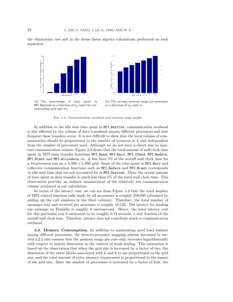
Figure 4.4(a) shows that the percentage of wall clock time spent in MPI Barrierincreases moderately as more processors are used to solve larger problems. Suchincrease is due primarily to the increase in the length of the critical path in both
22 L. LIN, C. YANG, J. LU, L. YING AND W. E
the elimination tree and in the dense linear algebra calculations performed on eachseparator.
(a) The percentage of time spent inMPI Barrier as a function of np (and the cor-responding grid size m).
(b) The average memory usage per processoras a function of np and m.
Fig. 4.4. Communication overhead and memory usage profile
In addition to the idle wait time spent in MPI Barrier, communication overheadis also affected by the volume of data transfered among different processors and howfrequent these transfers occur. It is not difficult to show that the total volume of com-munication should be proportional to the number of nonzeros in L and independentfrom the number of processors used. Although we do not have a direct way to mea-sure communication volume, Figure 4.3 shows that the total amount of wall clock timespent in MPI data transfer functions MPI Send, MPI Recv, MPI ISend, MPI Reduce,MPI Bcast and MPI Allreduce etc. is less than 5% of the overall wall clock time fora 16-processor run on a 4, 095× 4, 095 grid. Some of the time spent in MPI Recv andcollective communication functions such as MPI Reduce and MPI Bcast correspondsto idle wait time that are not accounted for in MPI Barrier. Thus, the actual amountof time spent in data transfer is much less than 5% of the total wall clock time. Thisobservation provides an indirect measurement of the relatively low communicationvolume produced in our calculation.
In terms of the latency cost, we can see from Figure 4.3 that the total numberof MPI related function calls made by all processors is roughly 258,000 (obtained byadding up the call numbers in the third column). Therefore, the total number ofmessages sent and received per processor is roughly 16,125. The latency for sendingone message on Franklin is roughly 8 microsecond. Hence, the total latency costfor this particular run is estimated to be roughly 0.13 seconds, a tiny fraction of theoverall wall clock time. Therefore, latency does not contribute much to communicationoverhead.
4.4. Memory Consumption. In addition to maintaining good load balanceamong different processors, the data-to-processor mapping scheme discussed in sec-tion 3.2.2 also ensures that the memory usage per core only increases logarithmicallywith respect to matrix dimension in the context of weak scaling. This estimation isbased on the observation that when the grid size is increased by a factor of two, thedimension of the extra blocks associated with L and D to are proportional to the gridsize, and the total amount of extra memory requirement is proportional to the squareof the grid size. Since the number of processors is increased by a factor of four, the

FAST PARALLEL ALGORITHM FOR SELECTED INVERSION 23
extra memory requirement stays fixed regardless of the grid size. This logarithmicdependence is clear from Figure 4.4(b), where average memory cost per core withrespect to number of processors is shown. The x-axis is plotted in logarithmic scale.
5. Application to electronic structure calculation of 2D rectangularquantum dots. In this section, we show how the algorithm and implementation wedescribed in section 3 can be used to speed up electronic structure calculations withinthe density functional theory (DFT) framework [18, 20]. The example we use here isa 2D electron quantum dot confined in a rectangular domain, a model investigated in[36]. This model is also provided in the test suite of the Octopus software [4], whichwe use for comparison.
The most time consuming part of a DFT electronic structure calculation is theevaluation of the electron density
ρ = diag(fβ,µ(H)), (5.1)
where fβ,µ(t) = 2/(1 + eβ(t−µ)) is the Fermi-Dirac distribution function with β beinga parameter that is proportional to the reciprocal of the temperature and µ beingthe chemical potential. The symmetric matrix H in (5.1) is a discretized Kohn-ShamHamiltonian [30] defined as
H = −12∆ + VH(r) + Vxc(r) + Vext, (5.2)
where ∆ is the Laplacian, VH is the Hartree potential, Vxc is a 2D exchange-correlationpotential constructed via the local density approximation (LDA) theory [3, 30] andVext is an external potential that describes an infinite hard-wall confinement in thexy plane, i.e.,
Vext(x, y) =
{0, 0 ≤ x ≤ L, 0 ≤ y ≤ L;∞, elsewhere.
(5.3)
To simplify our experiment, we do not consider spin-polarization.The standard approach for evaluating (5.1) is to compute the invariant subspace
associated with a few smallest eigenvalues of H. This approach is used in Octopus[4], which is a real space electronic structure calculation software package.
An alternative way to evaluate (5.1) is to use a recently developed pole expansiontechnique [22, 24] to approximate fβ,µ. The pole expansion technique expresses theelectron density ρ as a linear combination of the diagonal of (H − (µ + zi)I)−1, i.e.
ρ ≈P∑
i=1
Im(
diagωi
H − (µ + zi)I
). (5.4)
Here Im (H) stands for the imaginary part of H. The parameters zi and ωi arethe complex shift and weight associated with the i-th pole respectively. They canbe chosen so that the total number of poles P is minimized for a given accuracyrequirement. At room temperature, the number of poles required in (5.4) is relativelysmall (less than 100). In addition to temperature, the pole expansion (5.4) alsorequires an explicit knowledge of the chemical potential µ, which must be chosen sothat the condition
trace(fβ,µ(H)) = ne (5.5)

24 L. LIN, C. YANG, J. LU, L. YING AND W. E
is satisfied. This can be accomplished by solving (5.5) using the standard Newton’smethod.
In order to use (5.4), we need to compute the diagonal of the inverse of a numberof complex symmetric (non-Hermitian) matrices H − (zi + µ)I (i = 1, 2, ..., P ). Theimplementation of the parallel selective inversion algorithm described in section 3 canbe used to perform this calculation efficiently, as the following example shows.
In this example, the Laplacian operator ∆ is discretized using a five-point stencil.A room temperature of 300K (which defines the value of β) is used in our calculation.The area of the quantum dot is L2. In a two-electron dot, setting L = 1.66A anddiscretizing the 2D domain with 31× 31 grid points yields an total energy error thatis less than 0.002Ha. When the number of electrons becomes larger, we increase thearea of the dot in proportion so that the average electron density is fixed. A typicaldensity profile with 32 electrons is shown in Figure 5.1. In this case, the quantum dotbehaves like a metallic system with a tiny energy gap around 0.08eV.
x
y
−6 −4 −2 0 2 4 6−6
−4
−2
0
2
4
6
Fig. 5.1. A contour plot of the density profile of a quantum dot with 32 electrons.
We compare the density evaluation (5.1) performed by both Octopus and the poleexpansion technique. In Octopus, the invariant subspace associated with the smallestne/2 + nh smallest eigenvalues of H is computed using a conjugate gradient (CG)like algorithm, where ne is the number of electrons in the quantum dot and nh is thenumber of extra states for finite temperature calculation. The value of nh dependson the system size and temperature. For example, in the case of 32 electrons 4 extrastates are necessary for the electronic structure calculation at 300K. In the poleexpansion approach, we use 80 poles in (5.4), which in general could give a relativeerror in electron density on the order of 10−7 (in L1 norm) [24].
In addition to using the parallel algorithm presented in section 3 to evaluate eachterm in (5.4), an extra level of coarse grained parallelism can be achieved by assigningeach pole to a different group of processors.
In Table 5.1, we compare the efficiency of the pole expansion technique for thequantum dot density calculation performed with the standard eigenvalue calculationapproach implemented in Octopus. The maximum number of CG iterations for com-puting each eigenvalue in Octopus is set to the default value of 25. We label the poleexpansion-based approach that uses the algorithm and implementation discussed insection 3 as PCSelInv, where the letter C stands for complex. The factor 80 in thelast column of Table 5.1 accounts for 80 poles used in (5.4). When a massive numberof processors are available, this pole number factor will easily result in a factor of80 reduction in wall clock time for the PCSelInv calculation, whereas such a perfect
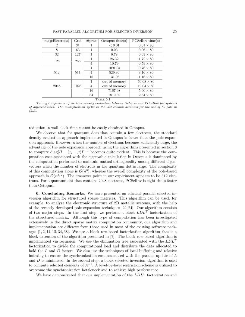
FAST PARALLEL ALGORITHM FOR SELECTED INVERSION 25
ne(#Electrons) Grid #proc Octopus time(s) PCSelInv time(s)
2 31 1 < 0.01 0.01× 80
8 63 1 0.03 0.06× 80
32 127 1 0.78 0.03× 80
128 2551 26.32 1.72× 80
4 10.79 0.59× 80
512 5111 1091.04 9.76× 80
4 529.30 3.16× 80
16 131.96 1.16× 80
2048 10231 out of memory 60.08× 80
4 out of memory 19.04× 80
16 7167.98 5.60× 80
64 1819.39 2.84× 80Table 5.1
Timing comparison of electron density evaluation between Octopus and PCSelInv for systemsof different sizes. The multiplication by 80 in the last column accounts for the use of 80 pole in(5.4).
reduction in wall clock time cannot be easily obtained in Octopus.We observe that for quantum dots that contain a few electrons, the standard
density evaluation approach implemented in Octopus is faster than the pole expan-sion approach. However, when the number of electrons becomes sufficiently large, theadvantage of the pole expansion approach using the algorithms presented in section 3to compute diag[H − (zi + µ)I]−1 becomes quite evident. This is because the com-putation cost associated with the eigenvalue calculation in Octopus is dominated bythe computation performed to maintain mutual orthogonality among different eigen-vectors when the number of electrons in the quantum dot is large. The complexityof this computation alone is O(n3), whereas the overall complexity of the pole-basedapproach is O(n3/2). The crossover point in our experiment appears to be 512 elec-trons. For a quantum dot that contains 2048 electrons, PCSelInv is eight times fasterthan Octopus.
6. Concluding Remarks. We have presented an efficient parallel selected in-version algorithm for structured sparse matrices. This algorithm can be used, forexample, to analyze the electronic structure of 2D metallic systems, with the helpof the recently developed pole-expansion techniques [22, 24]. Our algorithm consistsof two major steps. In the first step, we perform a block LDLT factorization ofthe structured matrix. Although this type of computation has been investigatedextensively in the direct sparse matrix computation community, our algorithm andimplementation are different from those used in most of the existing software pack-ages [1, 2, 14, 15, 34, 38]. We use a block row-based factorization algorithm that is ablock extension of the algorithm presented in [7]. The block row-based algorithm isimplemented via recursion. We use the elimination tree associated with the LDLT
factorization to divide the computational load and distribute the data allocated tohold the L and D factors. We also use the techniques of local buffering and relativeindexing to ensure the synchronization cost associated with the parallel update of Land D is minimized. In the second step, a block selected inversion algorithm is usedto compute selected elements of A−1. A level-by-level restriction scheme is utilized toovercome the synchronization bottleneck and to achieve high performance.
We have demonstrated that our implementation of the LDLT factorization and
26 L. LIN, C. YANG, J. LU, L. YING AND W. E
selected inversion calculation are very efficient. We have used our code to solve prob-lems defined on a 65, 535×65, 535 grid with more than four billions degrees of freedomon 4096 processors. The code exhibits an excellent weak scaling property.
When compared with the standard approach for evaluating the diagonal of aFermi-Dirac function of a Kohn-Sham Hamiltonian associated with a 2D electronquantum dot, the new pole-expansion technique that uses our algorithm to computethe diagonal of (H − ziI)−1 for a small number of poles zi’s is much faster, especiallywhen the quantum dot contains many electrons.
One of the key components that enable us to achieve high performance in ourimplementation is the parallel symbolic analysis procedure that makes explicit use ofthe grid and stencil geometry as well as the nested dissection partition and orderingtechnique. Due to space limitation, we left out the details of this step. Readers whoare interested in these details can find more information in [25]. This type of analysiscan be easily extended to regular 3D grids, so are our algorithm and implementationfor selected inversion calculations.
In order to design a selected inversion algorithm for problems that are defined onirregular grids (e.g., problems that are discretized by finite elements or some othertechniques), a general approach based on a general left-looking algorithm [34], a blockfan-out algorithm [37], or a multifrontal algorithm is more appropriate. A sequentialalgorithm has recently been developed for this general selected inversion [26]. Toachieve scalable parallel performance, a more general parallel symbolic analysis similarto that described in [41] must also be used. This is an area of research we are currentlypursuing.
Acknowledgements. This work was partially supported by DOE under Con-tract No. DE-FG02-03ER25587 and by ONR under Contract No. N00014-01-1-0674(L. L., J. L. and W. E), by an Alfred P. Sloan fellowship and a startup grant from theUniversity of Texas at Austin (L. Y.), and by the Director, Office of Science, Divisionof Mathematical, Information, and Computational Sciences of the U.S. Departmentof Energy under contract number DE-AC02-05CH11231 (C. Y.). The computationalresults presented were obtained at the National Energy Research Scientific ComputingCenter (NERSC), which is supported by the Director, Office of Advanced ScientificComputing Research of the U.S. Department of Energy under contract number DE-AC02-05CH11232. We would like to thank Esmond Ng and Sherry Li for helpfuldiscussion.
References.[1] P. Amestoy, I. Duff, J.-Y. L’Excellent, and J. Koster, A fully asynchronous multifrontal solver
using distributed dynamic scheduling, SIAM J. Matrix Anal. and Appl. 23 (2001), 15–41.[2] C. Ashcraft and R. Grimes, SPOOLES: An object-oriented sparse matrix library, Ninth SIAM
conference on parallel processing, 1999.[3] C. Attaccalite, S. Moroni, P. Gori-Giorgi, and G. Bachelet, Correlation energy and spin polar-
ization in the 2d electron gas, Phys. Rev. Lett. 88 (2002), 256601.[4] A. Castro, H. Appel, M. Oliveira, C. Rozzi, X. Andrade, F. Lorenzen, M. Marques, E. Gross,
and A. Rubio, Octopus:a tool for the application of time-dependent density functional theory,Phys. Stat. Sol. B 243 (2006), 2465–2488.
[5] T. Cormen, C. Leiserson, R. Rivest, and C. Stein, Introduction to algorithms, 3rd ed., MITPress, 2009.
[6] S. Datta, Electronic transport in mesoscopic systems, Cambridge Univ Pr, 1997.[7] T. Davis, Algorithm 849: A concise sparse Cholesky factorization package, ACM Trans. Math.
Software 31 (2005), 587–591.[8] I. Duff and J. Reid, The multifrontal solution of indefinite sparse symmetric linear systems,
ACM Trans. Math. Software 9 (1983), 302–325.[9] , Direct methods for sparse matrices, Oxford University, London, 1987.

FAST PARALLEL ALGORITHM FOR SELECTED INVERSION 27
[10] E. Economou, Green’s functions in quantum physics, Springer Berlin, 2006.[11] A. Erisman and W. Tinney, On computing certain elements of the inverse of a sparse matrix,
Numer. Math. 18 (1975), 177.[12] J. George and J. Liu, Computer solution of large sparse positive definite systems, Prentice-Hall,
Englewood Cliffs, NJ, 1981.[13] J. George, Nested dissection of a regular finite element mesh, SIAM J. Numer. Anal. 10 (1973),
345–363.[14] A. Gupta, G. Karypis, and V. Kumar, Highly scalable parallel algorithms for sparse matrix
factorization, IEEE Trans. Parallel Distrib. Syst. 8 (1997), 502–520.[15] A. Gupta, WSMP: the Watson Sparse Matrix Package, IBM Research Report (1997), no. RC
21886(98462).[16] J. Gustafson, Reevaluating Amdahl’s law, Comm. ACM 31 (1988), 532–533.[17] M. Heath, E. Ng, and B. Peyton, Parallel algorithms for sparse linear systems, SIAM Rev. 33
(1991), 420–460.[18] P. Hohenberg and W. Kohn, Inhomogeneous electron gas, Phys. Rev. 136 (1964), B864.[19] Cray Inc., Using cray performance analysis tools, Cray Inc., 2009.[20] W. Kohn and L. Sham, Self-consistent equations including exchange and correlation effects,
Phys. Rev. 140 (1965), A1133.[21] S. Li, S. Ahmed, G. Klimeck, and E. Darve, Computing entries of the inverse of a sparse matrix
using the FIND algorithm, J. Comput. Phys. 227 (2008), 9408 –9427.[22] L. Lin, J. Lu, R. Car, and W. E, Multipole representation of the Fermi operator with application
to the electronic structure analysis of metallic systems, Phys. Rev. B 79 (2009), 115133.[23] L. Lin, J. Lu, L. Ying, R. Car, and W. E, Fast algorithm for extracting the diagonal of the
inverse matrix with application to the electronic structure analysis of metallic systems, Comm.Math. Sci. (accepted).
[24] L. Lin, J. Lu, L. Ying, and W. E, Pole-based approximation of the Fermi-Dirac function, ChineseAnn. Math Ser. B (in press).
[25] L. Lin, C. Yang, J. Lu, L. Ying, and W. E, A fast parallel algorithm for selected inversionof structured sparse matrices with application to 2d electronic structure calculations, TechnicalReport LBNL-2677E, Lawrence Berkeley National Laboratory, 2009.
[26] L. Lin, C. Yang, J. Meza, J. Lu, L. Ying, and W. E, SelInv – an algorithm for selected inversionof a sparse symmetric matrix, in preparation (2009).
[27] J. Liu, The role of elimination trees in sparse factorization, SIAM J. Matrix Anal. Appl. 11(1990), 134.
[28] , A generalized envelope method for sparse factorization by rows, ACM Trans. Math.Software 17 (1991), 112–129.
[29] , The multifrontal method for sparse matrix solution: Theory and practice, SIAM Rev.34 (1992), 82–109.
[30] R. Martin, Electronic structure – basic theory and practical methods, Cambridge UniversityPress, 2004.
[31] C. Moler, Numerical computing with MATLAB, SIAM, 2004.[32] S. Moore, P. Mucci, J. Dongarra, S. Shende, and A. Malony, Performance instrumentation and
measurement for terascale systems, Lecture notes in computer science, 2003, pp. 53–62.[33] E. Ng and B. Peyton, A supernodal Cholesky factorization algorithm for shared-memory multi-
processors, SIAM J. Sci. Comput. 14 (1993), 761.[34] , Block sparse Cholesky algorithms on advanced uniprocessor computers, SIAM J. Sci.
Comput. 14 (1993), 1034.[35] D. Petersen, S. Li, K. Stokbro, H. Sørensen, P. Hansen, S. Skelboe, and E. Darve, A hybrid
method for the parallel computation of Green’s functions, J. Comput. Phys. 228 (2009), 5020–5039.
[36] E. Rasanen, H. Saarikoski, V. Stavrou, A. Harju, M. Puska, and R. Nieminen, Electronic struc-ture of rectangular quantum dots, Phys. Rev. B 67 (2003), 235307.
[37] E. Rothberg and A. Gupta, An efficient block-oriented approach to parallel sparse choleskyfac-torization, SIAM J. Sci. Comput. 15 (1994), 1413–1439.
[38] O. Schenk and K. Gartner, On fast factorization pivoting methods for symmetric indefinitesystems, Elec. Trans. Numer. Anal. 23 (2006), 158–179.
[39] R. Schreiber, A new implementation of sparse Gaussian elimination, ACM Trans. Math. Soft-ware 8 (1982), 256–276.
[40] D. Skinner and W. Kramer, Understanding the causes of performance variability in HPC work-loads, IEEE international symposium on workload characterization, IISWC05, 2005.
[41] E. Zmijewski and J. R. Gilbert, A parallel algorithm for sparse symbolic Cholesky factorizationon a multiprocessor, Parallel Comput. 7 (1988), 199–210.