The Author(s) BMC Bioinformatics 2016, (Suppl 1):510DOI 10.1186/s12859-016-1365-2

RESEARCH Open Access

A fast exact sequential algorithm for thepartial digest problem

Mostafa M. Abbas1* and Hazem M. Bahig2*

From 15th International Conference On Bioinformatics (INCOB 2016)Queenstown, Singapore. 21-23 September 2016

Abstract

Background: Restriction site analysis involves determining the locations of restriction sites after the process of digestionby reconstructing their positions based on the lengths of the cut DNA. Using different reaction times with a single enzymeto cut DNA is a technique known as a partial digestion. Determining the exact locations of restriction sites following apartial digestion is challenging due to the computational time required even with the best known practical algorithm.

Results: In this paper, we introduce an efficient algorithm to find the exact solution for the partial digest problem. Thealgorithm is able to find all possible solutions for the input and works by traversing the solution tree with abreadth-first search in two stages and deleting all repeated subproblems. Two types of simulated data, randomand Zhang, are used to measure the efficiency of the algorithm. We also apply the algorithm to real data for theLuciferase gene and the E. coli K12 genome.

Conclusion: Our algorithm is a fast tool to find the exact solution for the partial digest problem. The percentage ofimprovement is more than 75% over the best known practical algorithm for the worst case. For large numbers of inputs,our algorithm is able to solve the problem in a suitable time, while the best known practical algorithm is unable.

Keywords: Restriction site analysis, Digestion process, Partial digest problem, DNA, Bioinformatics algorithm, Breadth first search

BackgroundIn 1970, Hamilton Smith discovered that long DNA mole-cules could be digested into a set of restriction fragmentsby the restriction enzyme HindII based on the occurrenceof restriction sites with the sequences GTGCAC orGTTAAC [1]. Since that time, restriction enzymes haveplayed a crucial role in many biological experiments, in-cluding genome editing [2], gene cloning [3], protein ex-pression [4, 5] and genome mapping [6–11]. Restrictionenzymes are commonly used to physically map genomes.In physical mapping, the restriction enzymes are used tocut a DNA molecule at restriction sites with the goal ofidentifying the locations of the restriction sites after diges-tion. Their positions in the genome are determined byanalyzing the lengths of the digested DNA. Based on theexperimental assumptions of digestion, there are two main

* Correspondence: mohamza@hbku.edu.qa; hazem.m.bahig@gmail.com1Qatar Computing Research Institute, Hamad Bin Khalifa University, Doha,Qatar2Computer Science Division, Department of Mathematics, Faculty of Science,Ain Shams University, Cairo 11566, Egypt

© The Author(s). 2016 Open Access This articInternational License (http://creativecommonsreproduction in any medium, provided you gthe Creative Commons license, and indicate if(http://creativecommons.org/publicdomain/ze

types of digestions, a partial digest [9] and a double digest[10]. Constructing an accurate physical map following apartial digestion is a fundamental problem in genome ana-lysis. In this work, we consider the partial digestion.In a partial digestion experiment, one restriction enzyme

is used to cut one or more target DNA molecules at severalspecific restriction site. The digestion results in a collectionof short DNA fragments, and the lengths of these frag-ments are recorded in multiset A. Attempting to recon-struct the locations of the restriction sites in the targetDNA molecules using multiset A is known as the PartialDigest Problem, PDP. Some modifications have been intro-duced into the partial digestion process to produce simpli-fied variants of PDP. These variants include: the simplifiedpartial digest problem, SPDP [12], the labeled partial digestproblem, LPDP [13] and the probed partial digest problem,PPDP [14]. In this work, we consider the PDP.Several algorithms [15–20] have been developed to solve

the PDP. Some of these algorithms have short runningtimes, but the solutions are not exact. These algorithms

le is distributed under the terms of the Creative Commons Attribution 4.0.org/licenses/by/4.0/), which permits unrestricted use, distribution, andive appropriate credit to the original author(s) and the source, provide a link tochanges were made. The Creative Commons Public Domain Dedication waiverro/1.0/) applies to the data made available in this article, unless otherwise stated.

The Author(s) BMC Bioinformatics 2016, (Suppl 1):510 Page 140 of 295

[15–17] are based on heuristic and approximation strat-egies. Other algorithms require a long running time in theworst case, but the solution is exact for any instance.These algorithms [18–20] are based on brute force orbranch and bound strategies.In this research paper, we describe an algorithm with a

suitable run time that generates an exact solution for thePDP. The previous algorithms that yield an exact PDP solu-tion can be divided into impractical and practical types. Theimpractical solutions are based on the brute force strategyand polynomial factorization [19]. The best known practicalalgorithm for PDP is the algorithm proposed by Skiena et al.[20], which is based on the branch and bound strategy. Thealgorithm is practical because the running time of the algo-rithm is O (n2 log n) for an average case, while exponentialamounts of time were required for the worst case.

Problem formulation and related definitionsBefore we give the formal definition of the PDP, we needthe following related definitions.Definition 1 [21]: The difference of two multisets D

and L denoted by D\L such that D\L = {x|x ∈D andC(D\L, x) =C(D, x) −C(L, x) > 0}, where C (D, x) denotes thenumber of occurrences of element x ∈D in D.Definition 2 [21]: The sum or (disjoint union) of

two multisets D and L denoted by D ∪+ L such thatD ∪+ L = {x|x ∈D or x ∈ L and C (D ∪+ L, x) = C (D, x) +C (L, x)}.Definition 3 [22]: The differences of element y and a set

X denoted by Δ (y,X) such that Δ(y,X) = {|y − xi| : xi ∈X}.Definition 4 [22]: The differences for a set X, denoted by

ΔX, is a multiset such that: ΔX = {|xj − xi|, 0 ≤ i < j ≤ n − 1}.Remark 1: We can write ΔX in another form ΔX =

i = 0n − 1 ∪+ Δ (xi, (X\xi)), where X = {x0, x1,…, xn − 1}.The Partial Digest Problem, PDP [11]: Given a multiset

of N ¼ n2

� �positive integers D = {d0, d1, d2, …, dN− 1}. Is

there a set of n integers X = {x0, x1, x2, …, xn − 1} such thatΔX =D ?.We also need two propositions. The first proposition is used

to give another formula for the difference between three mul-tiple sets. The formula will be used to prove the correctness ofour proposed method. The second proposition is used to illus-trate how to construct an example for the worst case, whichleads to an exponential time for Skiena’s algorithm [23].Proposition 1: Let D, L and Z be three multisets, then

(D\L)\Z =D\(L ∪+ Z).Proposition 2 [23]: Let 0 < ε < 1

12 n , A1 = {1 − nε,…,1 − 2ε, 1 − ε}, A2 = {ε, 2ε,…, nε}, A3 = {(n + 1)ε, (n + 2)ε,…,2nε}, A4 = {(2n + 1)ε, (2n + 2)ε,…, 3nε}, A5 = {1 − 3nε,…,1− (2n + 2)ε, 1− (2n + 1)ε} and D = F ∪G where F and G aredisjoint sets satisfying F ∪G* =A3 and G* = {1− g| ∀ g ∈G}.Let A=A1 ∪A2 ∪A4 ∪A5 ∪D ∪ {0, 1}, we can choose D such

that giving ΔA to Skiena’s algorithm will take it at leastΩ(2n − 1) time to find A.

MethodsIn this section, we present three algorithms. The firstone is the best previous practical algorithm, while theother two algorithms are the proposed algorithms.

Best previous practical algorithmThe main goal of PDP is to reconstruct the elements, xi, froma multiset, D, of N= n (n− 1)/2 integers by finding a set Xsuch that ΔX = D. The best known algorithm for solving thePDP is based on the branch and bound strategy. The mainidea of this algorithm is to construct the set X incrementally.The algorithm is based on the depth-first search algorithmwith two bounding conditions. We refer to this method asAlgorithm BBd (branch and bound based on depth).

ObservationFigure 1 represents the execution of the algorithm BBdon D = {1, 2, 2, 3, 5, 6, 7, 8, 8, 10}. In the figure, we usethe following notations.

Fig. 1 Tracing the BBd algorithm on D = {1, 2, 2, 3, 5, 6, 7, 8, 8, 10}

The Author(s) BMC Bioinformatics 2016, (Suppl 1):510 Page 141 of 295

i. Each node in the solution tree for the PDPrepresents a pair of sets (Dk

i , Xki ) where the index k

represents the level number, and the index irepresents the node number in the level k.

ii. The number t inside the circle at the top right of eachnode represents the t-th calling for the procedure Place.

iii. The symbol “⊥” is used when the current node doesnot generate any new elements.

It is clear that at the level 0, the root contains the mul-tiset D0

0 = {1, 2, 2, 3, 5, 6, 7, 8, 8} and the set X00 = {0, 10}.

In general, X00 = {0, width} and D0

0 =D \ {width}, where Dis the input of the PDP. Additionally, each node (Dk

j , Xkj )

at the level k, k > 0, of the solution tree generates at mosttwo nodes at the level k + 1 as follows:

1. Add an element y to Xkj to generate Xk + 1

i = Xkj ∪ {y}.

2. Remove the elements of Δ (y,Xkj ) from Dk

j to generateDk + 1i =Dk

j \Δ(y,Xkj ).

where y =Max (Dkj ) or y = width ‐Max(Dk

j ). We also ob-serve from Fig. 1 the following:

1. There are two identical subproblems (D20, X2

0) and (D21, X2

1),such that D2

0 =D21 = {1, 3, 5, 7} and X2

0 =X21 = {0, 2, 8, 10}.

2. The two identical subproblems lead to two identicalsolutions, {0, 2, 7, 8, 10} and {0, 2, 3, 8, 10}.

First proposed methodIn this subsection, we propose an efficient method that re-duces the running time of the PDP. The method is based ontraversing the solution tree for the PDP using the breadth-first strategy instead of the depth-first strategy. We also con-sider the two bounding conditions that are used in algorithmBBd. Moreover, we remove all identical subproblems at thesame level. The main steps of our method are as follows:

1. Build the solution tree for the PDP using thebreadth-first strategy, level by level.

2. Before creating the nodes of the new level, we removeall repeated nodes existing in the current level such thatany node appears only one time in the current level.

Algorithm BBb (branch and bound based on breadth)shows the steps of our proposed method to solve thePDP. The input of the algorithm is the multiset D thatconsists of n (n − 1)/2 elements. Initially the algorithmstarts with two sets and two lists. The two sets are X0

0 = {0,width} and D0

0 =D \ {width}. The two lists are LX = {X00} and

LD = {D00}. In general, LD and LX represent the lists of sets,

Dkj and Xk

j , respectively, at the current level, k, of the solu-tion tree. The main step of the proposed algorithm is awhile loop that represents the number of levels in the solu-tion tree for the PDP. In each iteration k of the while loop,we will generate the elements of the next level, k + 1, bycalling the procedure GenerateNextLevel (LD, LX, S), k ≥ 0.The inputs of the procedure are three lists of sets, LD, LXand S, for the current level k. The outputs of the procedureare three lists of sets, LD, LX and S, for the level k + 1.The body of the procedure GenerateNextLevel consists

of an initialization and a loop. In the initialization, we willuse two auxiliary lists, ALD and ALX, which contain thesets Dk + 1

j and Xk + 1j , respectively, for the next level in the

solution tree. The initial value of the two lists is empty.The main loop in the GenerateNextLevel procedure rep-resents the process of generating the elements of the nextlevel and storing it in the two auxiliary lists ALD and ALX.Each pair of sets, Dk

i ∈ LD and Xki ∈ LX, will generate at

most two pairs of sets, as follows:

(i) Dk + 1j =Dk

i \Δ (y, Xki ) and Xk + 1

j = Xki ∪ {y } if the

condition Δ (y , Xki )⊆Dk

i is true.(ii)Dk+1

l =Dki \Δ (width ‐ y, Xk

i ) and Xk+1l =Xk

i ∪ {width ‐ y }if the condition Δ (width ‐ y , Xk

i )⊆Dki is true.

The two sets, Xk + 1j and Dk + 1

j and in a similar way,Xk + 1l and Dk + 1

l , will be added to the auxiliary lists ALXand ALD, respectively if set Xk + 1

j does not exist in listALX.The main loop of the GenerateNextLevel procedure

will terminate when list LD is empty. This means that allof the elements of the current level k are replaced bynew elements in the next level k + 1. In this case, we as-sign the lists ALD and ALX to LD and LX, respectively.Figure 2 illustrates how this idea works.

The Author(s) BMC Bioinformatics 2016, (Suppl 1):510 Page 142 of 295

Now, we investigate how to test the equality betweentwo nodes (Dk

i , Xki ) and (Dk

j , Xkj ) in the solution tree for

the PDP. The test can be performed by comparing theequality between Dk

i and Dkj and the equality between Xk

i

and Xkj . The following theorems and corollary prove that

the two nodes (Dki , Xk

i ) and (Dkj , Xk

j ) are equal if the setXki is equal to the set Xk

j .Theorem 1: Given a subproblem (Dk

i , Xki ) in the solu-

tion tree for the PDP, the relation Dki =D \ ΔXk

i is valid,where k ≥ 0, D is the input of the PDP, Dk

i is a modifiedversion of D produced by removing some of its ele-ments and Xk

i contains k + 2 elements of the candidatesolution.Proof: We will prove the theorem using mathematical

induction.First, we prove that the relation is true at k = 0.The algorithm starts by finding the maximum ele-

ments of the set D, width, and updates the value of thesets D and X. So, X0

0 = {0, width} and D00 = D\{width}.

From the definition of Δ, we have, ΔX00 = {width}. There-

fore, D00 = D\ΔX0

0.Second, we assume that the relation is true at k (i.e.,

Dki = D\ΔXk

i ).Third, we prove that the relation is true at k + 1.From the algorithm, the set Dk + 1

j can be constructedfrom a node at level k, say (Dk

i , Xki ). Therefore, Dk + 1

j =Dki \Δ (y, Xk

i ) and Xk+ 1j =Xk

i ∪ {y}. This implies that Dk+ 1j =

(D \ ΔXki )\Δ(y,Xk

i ), because Dki =D \ ΔXk

i . Therefore, Dk+1j =

D \ (ΔXki ∪+Δ(y,Xk

i )) (from Proposition 1). From Definition 4and because Xk+1

j = {y} ∪Xki , then Dk+1

j =D \ ΔXk+1j .

Theorem 2: If there are two subproblems (Dki , Xk

i )and (Dk

j , Xkj ) such that Xk

i = Xkj , then Dk

i =Dkj .

Proof: From Theorem 1, the following equations arevalid Dk

i =D\ΔXki and Dk

j =D\ΔXkj , for the subproblems

(Dki , Xk

i ) and (Dkj , Xk

j ), respectively. Because Xki = Xk

j , thenDki =D\ΔXk

i =D\ΔXkj =Dk

j .Corollary 1: If there are two subproblems (Dk

i , Xki )

and (Dkj , Xk

j ) such that Xki = Xk

j , then (Dki , Xk

i ) = (Dkj , Xk

j ).

Final proposed algorithmWe proposed an enhanced version of algorithm BBb. Theproposed algorithm improves the running time and stor-age of the BBb algorithm especially for the worst case. Inthe proposed algorithm, we try to reduce the memoryconsumption of the BBb algorithm without increasing itsrunning time. The improved algorithm depends on thefollowing two steps:

1. Building the solution tree for the PDP until aspecific level α is reached by using the BBbalgorithm.

2. For each node in the level α, building the remaindersubtrees individually with the BBb algorithm.

Figure 3 represents the idea described above for theproposed algorithm. We called the algorithm BBb2,branch and bound based on breadth two times.

Fig. 2 Tracing the BBb algorithm on D = {1, 2, 2, 3, 5, 6, 7, 8, 8, 10}

The Author(s) BMC Bioinformatics 2016, (Suppl 1):510 Page 143 of 295

To determine the best value of α, we need to computethe memory complexity of the proposed algorithm for theworst case. Each node in level k will be replaced by atmost two nodes in the level k + 1, 0 ≤ k < α. Therefore, thetotal number of nodes at level α is 2α. In each node, westore two sets, Dα

i and Xαi , of total size O (n2). Hence, the

total amount of storage necessary to reach the level α isO (n2 2α) memory for BBb2. In the second step of theBBb2 algorithm, we apply BBb on each node individually.The maximum number of remaining levels is n − α and thetotal amount of memory required for the second step forthe worst case is O (n2 2n − α). Hence, the memory complex-ity of the BBb2 algorithm for the worst case is given by:

M αð Þ ¼ O n2 2α� �þ O n2 2n−α

� �

Let αM be the number of levels that lead to the mini-mum memory required by BBb2. The value of αM canbe computed by determining the number of levels, α,that minimizes the memory consumption M(α), for0 ≤ α ≤ n − 1.The Find_αM procedure computes the valueof αM for the instance n in O(n) time. The input of theprocedure is the size of the multiset D, N, and the out-put of the procedure is αM. From the size of the multisetD, we can compute the value of n by solving the

Fig. 3 Strategy of the BBb2 algorithm

quadratic equation n n−1ð Þ2 ¼ N . The pseudocode of the

Find_αM procedure is as follows:Procedure Find_αM (N, αM)Begin

1: n ¼ 1þ ffiffiffiffiffiffiffiffiffiffiffiffiffiffiffi1þ 8N

p

22: α ¼ αM ¼ 1

3: M ¼ n2 2α þ 2n−αð Þ

min

4. for α = 2 to n do

5: M ¼ n2 2α þ 2n−αð Þ6. if M <Mmin then

7: Mmin ¼ M

8: α ¼ α

M

9. end if

10. end for

End

The Author(s) BMC Bioinformatics 2016, (Suppl 1):510 Page 144 of 295

In Algorithm BBb2, we start by finding the value ofαM and then we build the solution tree until the level αMis reached by using the breadth-first strategy and delet-ing all similar elements. At the level αM, we have at most2αM elements. After obtaining these elements, we con-sider each node as a root and then expand this nodeusing the BBb algorithm. For the worst case, the numberof handled elements at levels αM + 1, αM +2, …,n are 2,22, …, 2n−αM respectively, while the number of handledelements during execution of the BBb algorithm at levelsαM + 1, αM + 2,…,n are 2αMþ1 , 2αMþ2 , …,2n respectively.Therefore, BBb2 reduces the memory required by theBBb algorithm.

Test methodologyIn this section, we present the methodology that is usedto evaluate the performance of the algorithms, BBd, BBband BBb2, according to their running times and memoryconsumptions.

Platform SpecificationWe implemented the algorithms on a Dual Octa-coreprocessor machine (Intel Xeon E5-2690) with 128 GBRAM. Each processor has a 2.9 GHz speed with 20 MBof cache. The algorithms were implemented in C++ pro-grams. The programs were compiled using g++ with the-O3 flag under 64-bit Red Hat Enterprise Linux 4.4. Inthe experiments, we used a single core only.

Simulated dataWe studied the performance of the three algorithms, BBd,BBb and BBb2, on different types of data and different

sized data sets. We used two types of data described inprevious studies. The first data set was a random data set(RD) [16], while the second data set is the Zhang data(ZD) [16, 17, 23]. The RD was used to measure the per-formance of the algorithm for an average case; while theZD was used to measure the performance of the algorithmfor the worst case. In terms of data set size, there are twofactors that affect the performance of the algorithms foreach data set. The first factor is the number of elements inthe set X, n, while the second factor is the values of the nelements, M (maximum elements of X).In the case of the RD, we assumed that there were n

restriction sites in the DNA segments distributed randomly.Each input instance of the simulated data is a multisetD = ΔX such that the set X contains n positive numbersrandomly selected and each number is less than or equalto M. In the ZD, the locations of the restriction sites wereselected randomly according to Proposition 2 [23].The values of n in the case of the RD are 100, 200, 300,…

and 1000, while the values of n in the case of ZD are 15, 20,25, 30,… and 90. The range of n for the ZD is small becausethe running time for the algorithm was greater than 1 daywhen n > 90. We also used different values of M as follows:M = n*q, where q = 10, 100, 1000 and 10,000.

Running time and memoryFor each value of n, we ran each algorithm 50 times withdifferent inputs for the RD. For the ZD, we reduced thisnumber to 20 due to the increased running time of thealgorithms, especially BBd. The running time for eachalgorithm for a fixed n represents the average time forall instances studied. If the running time of an algorithmwas greater than 24 h for an input instance then thealgorithm was terminated. Therefore, the value of thealgorithm for this input instance was omitted from thefigures and the results.We also measured the standard error of the mean (SEM)

and coefficient of variation (CV) for the three algorithmsfor RD and ZD. Finally, we used a non-parametric statis-tical test which is Wilcoxon-signed-rank test [24] to deter-mine if there are a significant differences between the threealgorithms in running time or memory consumption onRD and ZD. We applied the Wilcoxon-signed-rank test,at a significance level of 0.05, to the following pairs:BBd & BBb, BBd & BBb2 and BBb & BBb2 algorithmswith respect to running time and memory consumptionfor RD and ZD.We measured the running time in seconds using a C++

function. We also measured the memory consumed by thealgorithm in megabytes using the Linux command top.

Results and discussionThe results from measuring the running times of thethree algorithms on the simulated data are shown in

The Author(s) BMC Bioinformatics 2016, (Suppl 1):510 Page 145 of 295

Fig. 4 and (Additional file 1: Figure F1) for the RD andFig. 5 for the ZD.In the case of the RD, the results showed that the run-

ning times of the proposed algorithms, BBb and BBb2,were less than the running time of BBd for all values ofn and M as shown in Fig. 4. For large values of n andsmall values of q, the BBd algorithm required a largeamount of time to find a solution, while the proposed al-gorithms, BBb and BBb2, found the solution in a suitabletime. For example, in the case of n ≥ 300 and M = n * 10,the running time for the BBd algorithm was greater than24 h, while both proposed algorithms found the solutionin time less than 13 min, as shown in Fig. 4a and b.However, the difference in running times between theBBd algorithm and the proposed algorithms, BBb andBBb2, decreased with increasing values of M. This behav-ior is attributed to the probability of repeated subproblemsdecreasing with increasing values of M. Therefore, bothalgorithms, BBb and BBb2, spend a large amount of timechecking for the repetition of elements with a low prob-ability of repetitions. Additionally, for small M valuesthe probability of repeated subproblems is high,thereby increasing the running time of the BBd algo-rithm. If we fixed the value of n, the running time forall algorithms decreased with increasing M values asshown in (Additional file 1: Figures F1 a-c). Both proposedalgorithms behaved similarly with increasing M values.We also observed that the difference in the running times

Fig. 4 Running times of the BBd, BBb and BBb2 algorithms for the RD. Thegreater than the maximum value of y-axis or 24 h

for two successive values of M is relatively small for bothproposed algorithms (especially when M is large) as shownin (Additional file 1: Figures F1 b and c). On the otherhand, the difference in the running times for the BBd algo-rithm for two successive values of M is large when M =n * 100 and M = n * 1000 as shown in (Additional file 1:Figure F1a). Finally, we found that there was little dif-ference, increasing or decreasing, between the runningtimes of BBb and BBb2 for all values of n and M. Ingeneral, with large values of n and M, the BBb2 algo-rithm was faster than the BBb algorithm. For example,in the case of n ≥700 and M = n * q and q = 1000 and10,000, BBb2 was slightly better than BBb.For the ZD, there was no change in the running time

when we used different values of M for the three algo-rithms. Therefore, we used the ZD with the M value fixedat M = n*1000. The consistent performance of the algo-rithms using the ZD with different values of M was due tothe systematic selection of the elements of A according toProposition 2.The performance of the three algorithms for the Zhang

data set instances is given in Fig. 5. We observed that therunning time of BBb2 was less than BBb and BBb was lessthan BBd for all instances. The percentage of running timeimprovement for BBb and BBb2 with respect to BBdincreased with increasing n. In our studied cases, therunning time was improved by at least 75%. Moreover,the BBd and BBb algorithms cannot solve any instances

line for BBd algorithm is not complete because the running time is

Fig. 6 Memory consumed of BBd, BBb, and BBb2 algorithms on ZD.The values on the y-axis are in log-scale

Fig. 5 Running times of the BBd, BBb and BBb2 algorithms for the ZD. The values on the y-axis are in log-scale

The Author(s) BMC Bioinformatics 2016, (Suppl 1):510 Page 146 of 295

with n ≥ 60 and n ≥ 80 in time less than 24 h respect-ively. In the other side, the BBb2 algorithm solves anyinstance with n≤90 in time less than 24 h.The improved running time of BBb algorithm can be

attributed to its reduction of the number of subproblemshandled at the levels αM + 1, αM + 2,…,n in the solutiontree for the PDP. Therefore, the time spent checkingsubproblem repetition is reduced.The results of measuring SEM and CV for the running

time of the three algorithms are shown in (Additionalfile 2: Tables S1–S5) for RD and ZD. The results showthat the values of SEM and CV for BBd algorithm werevery large compared to the values of SEM and CV forBBb and BBb2 algorithms in case of RD. For the ZD, thevalues of SEM and CV of BBb and BB2 algorithms wereless than the values of SEM and CV of BBd algorithm inthe most instances. Moreover, the application of Wilcoxon-signed-rank test shows that there was a significant differ-ence between the following pairs of the algorithms asshown in (Additional file 2: Tables S6–S14):

i. BBd and BBb in case of RD and ZD.ii. BBd and BBb2 in case of RD and ZD.iii. BBb and BBb2 in case of ZD.

We also evaluated the algorithms in terms of theirmemory consumptions. The results of measuring thememory consumed by the three algorithms on the simu-lated data are shown in (Additional file 3: Figures F2 a–d)for the RD and Fig. 6 for the ZD. For the RD, the resultsshow that for small values of M such as M = n * 10 andn * 100, the BBb and BBb2 algorithms consumed lessmemory than the BBd algorithm. In the case of large Mvalues, the BBd algorithm consumed less memory than

the BBb and BBb2 algorithms, but small M values in-creased the number of repeated subproblems. Thus, thenumber of elements in each level is large for the BBdalgorithm. Therefore, the BBd algorithm consumed morememory than the two proposed algorithms. In general, thememory consumption of the BBb algorithm is a littlebetter than that of the BBb2 algorithm.For the ZD, less memory was consumed by BBb2 than

BBb for all instances. So, the BBb2 algorithm significantlyreduced the memory required by the BBb algorithm. Thepercentage of improvement in memory consumption ofBBb2 compared to BBb increases as n increases. In gen-eral, the memory required by the BBd algorithm is lessthan the BBb and BBb2 algorithms.The results of measuring SEM and CV for the memory

of the three algorithms are shown in (Additional file 4:Tables S15–S19) for the RD and the ZD. The resultsshow that there were differences, decreasing and increasing,

The Author(s) BMC Bioinformatics 2016, (Suppl 1):510 Page 147 of 295

in the values of SEM and CV of the three algorithms forthe RD. For the ZD, the values of SEM and CV of BBd al-gorithm were less than the proposed algorithms in the mostinstances. Moreover, the application of Wilcoxon-signed-rank test, see (Additional file 4: Tables S20-S28), shows thatthere was a significant difference between the followingpairs of the algorithms in the following cases:

i. BBd and BBb on ZD.ii. BBd and BBb2 on ZD.iii. BBb and BBb2 on ZD.

Real dataWe tested the final proposed BBb2 algorithm on real di-gestion experiments and simulated digestion experiments.

Luciferase geneWe extracted the data from a partial digestion of the lu-ciferase gene [25] of length 2009. The partial digestionwas performed with the enzyme TaqI, which cuts thegene at the tcga sequence motif. The output of the par-tial digestion process is the multiset D consisting of thedistances between the tcga locations on the luciferasegene, which is D = {9, 30, 100, 170, 293, 302, 393, 402,462, 562, 632, 732, 855, 864, 945, 954, 975, 984, 1025,1034, 1247, 1277, 1347, 1377, 1809, 1839, 1979, 2009}.Our proposed algorithms take the multiset D as inputand output two solutions in the set S = {{0, 170, 632, 732,1025, 1034, 1979, 2009}, {0, 30, 975, 984, 1277, 1377, 1839,2009}}. The solution X = {0, 30, 975, 984, 1277, 1377,1839, 2009}, represents the solution for the real data. Thismeans that the map of tcga on luciferase gene at thelocations 30, 975, 984, 1277, 1377, and 1839.

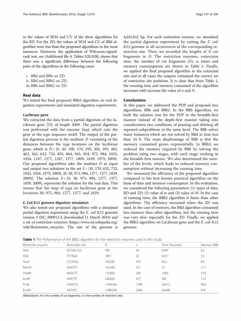
E. Coli K12 genome digestion simulationWe also tested our proposed algorithms with a simulatedpartial digestion experiment using the E. coli K12 genomeversion 3 (NC_000913.3, downloaded 11 March 2016) anda set of restriction enzymes (https://www.en.wikipedia.org/wiki/Restriction_enzyme). The size of the genome is

Table 1 The Performance of the BBb2 algorithm for the restriction e

Restriction enzyme Restriction site N

NotI GCGGCCGC 780

XbaI TCTAGA 1891

SmaI CCCGGG 103,285

BamHI GGATCC 135,460

HindIII AAGCTT 170,820

EcoRI GAATTC 228,826

PvuII CAGCTG 1,599,366

EcoRV GATATC 1,999,000

Abbreviations: N is the number of cut fragments, n is the number of restriction sites

4,641,652 bp. For each restriction enzyme, we simulatedthe partial digestion experiment by cutting the E. coliK12 genome at all occurrences of the corresponding re-striction site. Then, we recorded the lengths of N cutfragments in D. The restriction enzymes, restrictionsites, the number of cut fragments (N), n, times andmemory consumptions are shown in Table 1. Finally,we applied the final proposed algorithm to the extractedsets and in all cases the outputs contained the correct setof restriction site positions. It is clear that from Table 1,the running time and memory consumed of the algorithmincreases with increase the value of n and N.

ConclusionsIn this paper, we addressed the PDP and proposed twoalgorithms, BBb and BBb2. In the BBb algorithm, webuilt the solution tree for the PDP in the breadth-firstmanner instead of the depth-first manner taking intoconsideration two conditions of pruning and deleting allrepeated subproblems in the same level. The BBb solvesmany instances which are not solved by BBd in time lessthan 24 h. The main disadvantage of BBb is that thememory consumed grows exponentially. In BBb2, wereduced the memory required by BBb by solving theproblem using two stages, with each stage working inthe breadth-first manner. We also determined the num-ber of the levels, which leads to reduced memory con-sumption without increasing the running time.We measured the efficiency of the proposed algorithm

compared to the best known practical algorithm on thebasis of time and memory consumption. In the evaluation,we considered the following parameters: (1) types of data,RD and ZD; (2) value of n; and (3) value of M. In the caseof running time, the BBb2 algorithm is faster than otheralgorithms. The efficiency increased when the ZD wasused. In the case of memory, the BBd algorithm consumedless memory than other algorithms, but the running timewas very slow especially for the ZD. Finally, we appliedthe BBb2 algorithm on Luciferase gene and the E. coli K12genome.

nzymes used in this study

n Time (Seconds) Memory (MB)

40 0.007 0.2

62 0.017 3.6

455 56.2 8.9

521 72 11.7

585 138.6 13.6

677 360 15.5

1789 24,012 98.8

2000 42,840 979

The Author(s) BMC Bioinformatics 2016, (Suppl 1):510 Page 148 of 295

Additional files

Additional file 1: Supplementary figure. Figure F1 a–c represents thebehavior of the running time for BBd, BBb, and BBb2 algorithms withdifferent values of M and fixed value of n. The values on the y-axis are inlog-scale. In Figure a, the x-axis does not include the value of M = n * 10,because the running time is greater than 24 h. (PDF 8 kb)

Additional file 2: Supplementary data. Calculation of the Standard Errorof Mean (SEM), Coefficient of Variation (CV), and Wilcoxon Signed-Ranktest for the running time. Tables S1-S5. in Sheet 1 and 2, represent thecalculation of SEM and CV for the running time of BBd, BBb, and BBb2algorithms in case of random data and Zhang data respectively.Tables S6–S8. in Sheet 3, represent the Wilcoxon Signed-Rank testbetween BBd and BBb algorithms for the running time of Random andZhang data. Tables S9–S11. in Sheet 4, represent the Wilcoxon Signed-Ranktest between BBb and BBb2 algorithms for the running time of Randomand Zhang data. Tables S12–S14. in Sheet 5, represent the WilcoxonSigned-Rank test between BBd and BBb2 algorithms for the running time ofRandom and Zhang data. (XLS 168 kb)

Additional file 3: Supplementary figure. Figure F2 a–d represents thememory consumed for BBd, BBb, and BBb2 algorithms on random data.(PDF 88 kb)

Additional file 4: Supplementary data. Calculation of the Standard Errorof Mean (SEM), Coefficient of Variation (CV), and Wilcoxon Signed-Ranktest for the memory. Tables S15-S19. in Sheet 1 and 2, represent thecalculation of SEM and CV for the memory consumption of BBd, BBb, andBBb2 algorithms in case of random data and Zhang data respectively. TablesS20–S22. in Sheet 3, represents the Wilcoxon Signed-Rank test between BBdand BBb algorithms for the memory consumption of Random andZhang data. Tables S23–S25. in Sheet 4, represent the WilcoxonSigned-Rank test between BBb and BBb2 algorithms for the memoryconsumption of Random and Zhang data. Tables S26-S28. in Sheet 5,represent the Wilcoxon Signed-Rank test between BBd and BBb2 algorithmsfor the memory consumption of Random and Zhang data. (XLS 167 kb)

AcknowledgementsThe experimental study of this work was done where the first author wasat KINDI Center for Computing Research, College of Engineering, QatarUniversity, Doha, Qatar.

DeclarationsThis article has been published as part of BMC Bioinformatics Volume 17Supplement 19, 2016. 15th International Conference On Bioinformatics(INCOB 2016): bioinformatics. The full contents of the supplement areavailable online at https://www.bmcbioinformatics.biomedcentral.com/articles/supplements/volume-17-supplement-19.

FundingPublication charges for this article have been funded by Qatar ComputingResearch Institute (QCRI), Hamad Bin Khalifa University, Qatar Foundation.

Availability of data and materialsData used in the article are publicly available. Availability of software exists at:https://www.github.com/mostafa-abbas/PDP.

Authors’ contributionsBoth authors contributed to theoretical and practical study equally. Bothauthors wrote and approved the manuscript.

Competing interestsThe authors declare that they have no competing interests.

Consent for publicationNot applicable.

Ethics approval and consent to participateAll the datasets used in this study were obtained from open-access databases andpreviously published by other authors. No human or animal data were collected.Therefore, no informed consent forms were needed from this study.

Published: 22 December 2016

References1. Pevzner P. DNA physical mapping and alternating eulerian cycles in colored

graphs. Algorithmica. 1995;13(1–2):77–105.2. Baker M. Gene-editing nucleases. Nat methods. 2012;9(1):23–6.3. Sambrook J, Fritsch EF, Maniatis T. Molecular cloning: a laboratory manual. 2nd

ed. New York: Cold Spring Harbor Laboratory Press, Cold Spring Harbor; 1989.4. Liu Z, Ping-Chang Y. Construction of pET-32 α (+) vector for protein

expression and purification. N am j med sci. 2012;4(12):651–5.5. He X, Hull V, Thomas JA, Fu X, Gidwani S, Gupta YK, Black LW, Xu SY. Expression

and purification of a single-chain type IV restriction enzyme Eco94GmrSD anddetermination of its substrate preference. Sci rep. 2015;5:9747.

6. Narayanan P. Bioinformatics: A primer. New Age International. 2005. ISBN 10:8122416101, ISBN 13: 9788122416107.

7. Kalavacharla V, Hossain K, Riera-Lizarazu O, Gu Y, Maan SS, Kianian SF.Radiation hybrid mapping in crop plants. Adv agron. 2009;102:201–22.

8. Dear PH. Genome mapping. eLS 2001. John Wiley & Sons. doi:10.1038/npg.els.0001467.

9. Błażewicz J, Formanowicz P, Kasprzak M, Jaroszewski M, Markiewicz WT.Construction of DNA restriction maps based on a simplified experiment.Bioinformatics. 2001;17(5):398–404.

10. Paliswiat B, Pryputniewicz P. On the complexity of the double digestproblem. Control cybern. 2004;33(1):133–40.

11. Cieliebak M, Eidenbenz S, Penna P. Noisy data make the partial digestproblem NP-hard. Lect notes comput cci. 2003;2812:111–23.

12. Blazewicz J, Burke EK, Kasprzak M, Kovalev A, Kovalyov MY. Simplified partialdigest problem: enumerative and dynamic programming algorithms.IEEE/ACM trans comput biol bioinform. 2007;4(4):668–80.

13. Pandurangan G, Ramesh H. The restriction mapping problem revisited. Jcomput syst sci. 2002;65(3):526–44.

14. Karp RM, Newberg LA. An algorithm for analysing probed partial digestionexperiments. Comput appl biosci. 1995;11(3):229–35.

15. Dakic T: On the turnpike problem. PhD thesis, Simon Fraser University 2000,ISBN:0-612-61635-5.

16. Nadimi R, Fathabadi HS, Ganjtabesh M. A fast algorithm for the partialdigest problem. Jpn j ind appl math. 2011;28:315–25.

17. Ahrabian H, Ganjtabesh M, Nowzari-Dalini A, Razaghi-Moghadam-Kashani Z.Genetic algorithm solution for partial digest problem. Int j bioinform resappl. 2013;9(6):584–94.

18. Rosenblatt J, Seymour PD. The structure of homometric sets. SIAM j algebraicdiscrete meth. 1982;3(3):343–50.

19. Lemke P, Werman M. On the complexity of inverting the autocorrelationfunction of a finite integer sequence, and the problem of locating n pointson a line, given the (nC2) unlabelled distances between them. Technicalreport # 453. IMA: Minneapolis; 1988.

20. Skiena SS, Smith WD, Lemke P. Reconstructing sets from interpoint distances.SCG '90 Proceedings of the sixth annual symposium on Computationalgeometry, 332–9.

21. Syropoulos A. Mathematics of multisets. WMP '00 Proceedings of theWorkshop on Multiset Processing: Multiset Processing, Mathematical,Computer Science, and Molecular Computing Points of View. 2000;347–58.

22. Jones NC, Pevzner P. An introduction to bioinformatics algorithms. Chapter 4,83-123, MIT press 2004.

23. Zhang Z. An exponential example for a partial digest mapping algorithm.J comput biol. 1994;1(3):235–9.

24. Woolson RF. Wilcoxon Signed‐Rank Test. Wiley encyclopedia of clinical trials2008. doi:10.1002/9780471462422.eoct979.

25. Devine JH, Kutuzova GD, Green VA, Ugarova NN, Baldwin TO. Luciferasefrom the east European firefly luciola mingrelica: cloning and nucleotidesequence of the cDNA, overexpression in Escherichia coli and purification ofthe enzyme. Biochim biophys acta. 1993;1173(2):121–32.