A fast algorithm for equality-constrained quadratic programming on the alliant FX/8

Annals of Operations Research 14(1988) 225-243 225

A Fast Algorithm for Equality-Constrained

Quadratic Programming on the Alliant FX/8

S. Wright Mathematics Department,

Box 8205, North Carolina State University,

Raleigh, N,C. 27695-8205.

An efficient implementation of the null-space method for quadratic programming on the Alliant FX/8 computer is described. The most computationally significant operations in this method are the orthogonal factorization of the constraint matrix and corresponding similarity transformation of the Hessian, and the Cholesky factorization of the reduced Hessian matrix. It is shown how these can be implemented in such a way as to take full advantage of the Alliant's parallel/vector capabilities and memory hierarchy. Timing results are given on a set of test problems for which the data can be easily accommodated in core memory.

Note: Research partially supported by the Air Force office of Scientific Research under grant AFOSR-ISSA-870092 and the National Science Founda- tion under grant DMS-8619903.

1. INTRODUCTION Perhaps the simplest problem in nonlinear constrained optimization is the equality-constrained quadratic programming problem

rrfin -~xrGx + grx s.t. A rx = b, (1.1) xeR"

where GeR "×', gER", A e R n×t, beR n×t and O<~t<.n. Without loss of generality, G can be assumed to be symmetric. Techniques for solving (1.1) are weU-known (see, for example, FLFrCrmR [4], GILL, MURRAY and WRIGHT [5], CONN and GOULD [3], and the references in these works.) Here we consider one such method, the null-space or orthogonal factorization method, which is most often used when t is comparable in size to n. In this method, an orthonormal matrix which spans the null space of A r is found; this is used to elim- inate the constraints and reduce the dimensionality of the minimization problem to n - t. We describe in this paper an implementation of this method on the Alliant FX/8, which takes advantage of the special features of that machine. These features include a configuration of eight vector processing units, a 64 M byte main memory an a 128 K byte cache (fast-access) memory. As we show later, this architecture is more suitable for linear algebra which is based on matrix - - matrix operations, rather that the more usual matrix - -

© J.C. Baltzer A.G., Scientific Publishing Company

226 A fast algorithm for quadratic programming

vector constructs. The most time-consuming tasks in the algorithm have been structured with this in mind.

Besides being useful in its own right, (1.1) arises as a component of algorithms for the solution of more complicated optimization problems. This is true for active-set methods for inequality-constrained quadratic programming, and for general linearly- and nonlinearly-constrained optimization. In such methods, some subset of the inequality constraints is held to be active (i.e. satisfied at equality) at each iteration. If necessary the objective and/or constraint functions are simplified and a "subproblem" of the form (1.1) is obtained. The Lagrange multipliers of the constraints in (1.1) are useful in this context for making decisions regarding deletion of constraints from the active set. The multipliers are also important in sensitivity analysis, so it is desirable that they be available along with the solution of (1.1).

We assume in this paper that the matrix A in (1.1) has full rank, and that the second-order sufficient conditions are satisfied (that is, the projection of the Hessian G into the null space of A is positive defimte). If the projected Hessian has any negative eigenvalues, then the problem (1.I) has no bounded solution. The aim of this paper is to describe a highly-optimized implementation, rather than an algorithm which can handle all such eventualities. If degeneracy is observed in A, or if the projected Hessian is not positive definite, the code returns an error condition.

Section 2 deals with the programming environment; the Alliant's architecture is described in more detail. Also we discuss the basic linear algebra routines from the software library at the University of Illinois Center for Super- computing Research and Development (CSRD), which were used in this algorithm.

In section 3, the orthogonal factorization method is described in detail, and the two major computational tasks are identified. The first of these, namely the orthogonal factorization of A and the consequent application of a similarity transformation to the Hessian G, is discussed in section 4. We show how this task is implemented, and give timing comparisons with a more conventionally-coded "benchmark" algorithm which performs the same task. The second major task, the Cholesky factorization of the projected Hessian matrix, is discussed in section 5. Again, timing comparisons with a more con- ventional code are given. Timing results for the overall algorithm are presented in section 6. Finally, section 7 contains some concluding observations, and some planned future extensions to this work.

2. COMPUTATIONAL ENVIRONMENT The algorithm was implemented on the Alliant FX/8 vector multiprocessor system at Argonne National Laboratory and at the University of Illinois CSRD, making use of basic linear algebra routines which were written for this computer at the CSRD [1].

The Alliant FX/8 consists of eight vector processors (known as computational elements or CEs). Each CE has a scalar and a vector instruction set, with eight floating point vector registers. In vector mode, each CE executes

S. Wright 227

single-precision floating point operations at a peak rate of 11.8 million per second (that is, 11.8 Mflops). Thus the 8-processor configuation can achieve a peak rate of approximately 94 Mflops in single-precision arithmetic. The Eight CEs share a global physical memory of 64 Mbytes, and a 128 Kbyte write- back cache memory. Eight simultaneous accesses to the cache are allowed in each cycle of 170 ns.

The FORTRAN compiler attempts to detect pieces of code which could be vectorized and/or executed concurrently. Generally, in a nested-loop structure, the compiler attempts to vectorize the innermost loop, and execute the next- to-innermost loop in concurrent mode. Such optimization is not carried out if there is feedback from earlier iterations of a loop to later iterations ("data dependency"). Users can override the optimization process by placing compiler directives in their code.

From the viewpoint of a user who wants to restructure an algorithm for optimum efficiency on the AUiant, probably the most important feature is the small cache memory. When a piece of data (i.e. a matrix or vector elemen0 is read into the cache, it is desirable to use it as often as possible before repla- cing it with another element from the (slower) main memory. The aim should be to keep the ratio of floating point operations to data movements as large as possible. This leads to the use of matrix-matrix operations as the basic algo- rithmic unit, as the following simple example shows. Suppose there are two (Ln) × n matrices A and B, with L >> 1, and we wish to calculate A rB. Denoting columns of A and B by ai and bi respectively, one possible approach would be the following:

do j = l , n

do i = l , n

: afbj enddo

enddo

(2.D

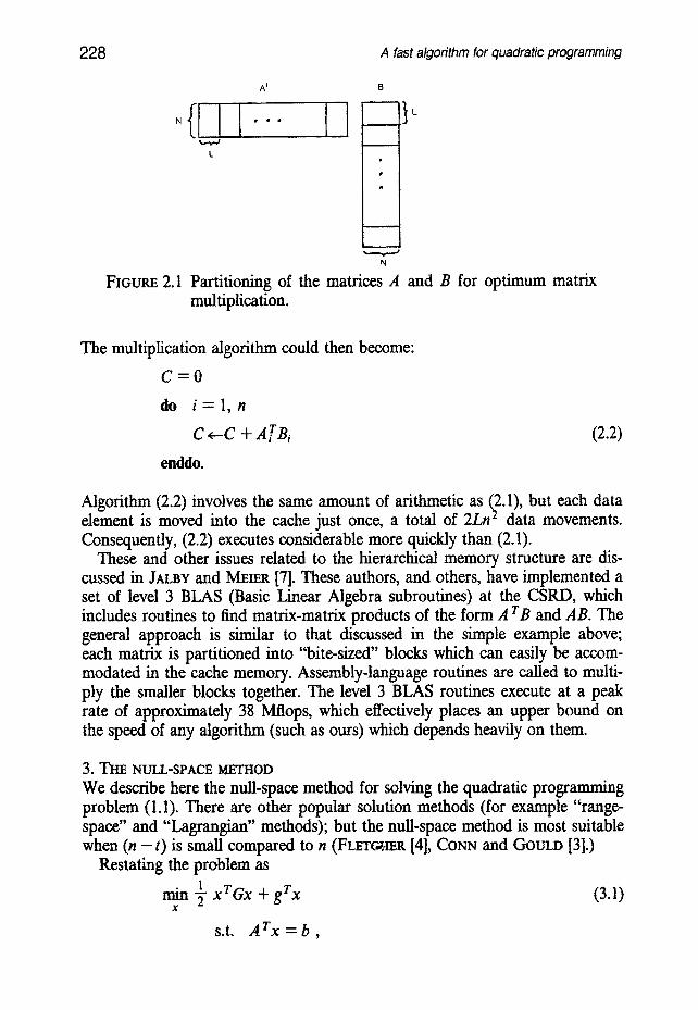
If the cache memory was just larse enough to hold the matrix C and the vec, tors ai and bj (approximately nZ+ 2Ln numbers) the algorithm (2.1) would require approximately n 2 movements of these vectors into the cache, or Ln 3 data movements overall. An alternative approach is to partition A and B into blocks of dimension L × n, as shown in Figure 2.1.

228

A t

L

A fast algorithm for quadratic programming

B

t L

N

FIGURE 2.1 Partitioning of the matrices A and B for optimum matrix multiplication.

The multiplication algorithm could then become:

C = 0

do i = l , n

C <--C + ATBi

enddo.

(2.2)

Algorithm (2.2) involves the same amount of arithmetic as (2.1), but each data element is moved into the cache just once, a total of 2Ln 2 data movements. Consequently, (2.2) executes considerable more quickly than (2.1).

These and other issues related to the hierarchical memory structure are discussed in JALBY and MEmR [7]. These authors, and others, have implemented a set of level 3 BLAS (Basic Linear Algebra subroutines) at the CSRD, which includes routines to find matrix-matrix products of the form A rB and AB. The general approach is similar to that discussed in the simple example above; each matrix is partitioned into "bite-sized" blocks which can easily be accommodated in the cache memory. Assembly-language routines are called to multiply the smaller blocks together. The level 3 BLAS routines execute at a peak rate of approximately 38 Mflops, which effectively places an upper bound on the speed of any algorithm (such as ours) which depends heavily on them.

3. TIlE NULL-SPACE METHOD We describe here the null-space method for solving the quadratic programming problem (1.1). There are other popular solution methods (for example "range- space" and "Lagrangian" methods); but the null-space method is most suitable when (n - t ) is small compared to n (FLETC.~ER [4], CONN and GOULD [3].)

Restating the problem as 1 rain -~ xrGx + grx (3.1)

X

s.t. A r x = b ,

S. Wright

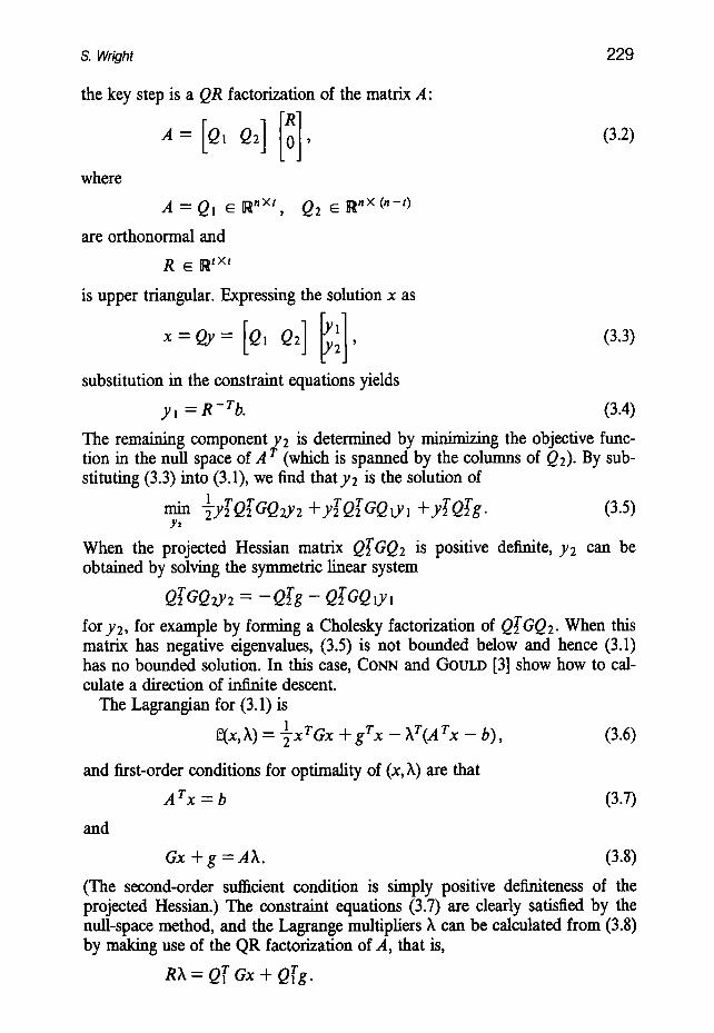
the key step is a QR factorization of the matrix A"

where

A = QI e R "xt, Q2 ~- Rnx (n-t)

are orthonormal and R ~. ~ t x t

is upper triangular. Expressing the solution x as

1I,] x=Q_.y= Q, Q2 2 '

229

(3.2)

(3.3)

RX = Q~ Gx + Qrg.

Cx + g = a x . (3.8)

(The second-order sufficient condition is simply positive defmiteness of the projected Hessian.) The constraint equations (3.7) are dearly satisfied by the nuU-space method, and the Lagrange multipliers h can be calculated from (3.8) by making use of the QR factorization of A, that is,

and

substitution in the constraint equations yields

Y ! = R - rb. (3.4)

The remaining component y2 is determined by minirnizing the objective func- tion in the null space of A (which is spanned by the columns of Q2). By sub- stituting (3.3) into (3.1), we find that Y2 is the solution of

1 T T T T nftn -fy2 02 GQ2,y2 + yT2 Q~GQlyl +y2 a2g. (3.5) Y~

When the projected Hessian matrix Qr2GQ2 is positive definite, y2 can be obtained by solving the symmetric linear system

arGa2y 2 = -Q~g - QrGQIy I

for y2, for example by forming a Cholesky factorization of QTGQ2. When this matrix has negative eigenvalues, (3.5) is not bounded below and hence (3.1) has no bounded solution. In this case, CoNN and GOULD [3] show how to calculate a direction of infinite descent.

The Lagrangian for (3.1) is

¢.(x,h) = l x r G x + grx -- hr(A rx -- b), (3.6)

and first-order conditions for optimality of (x, h) are that

A rx = b (3.7)


In summary, our implementation follows these steps:

ALGORITHM QPE (1) Factor A = Q ~0R], form QrGQ, Qrg.

(2) Solveyl = R - ' b (3) Form c : Qrg + (QrGQrl)y l (4) Cholesky factorization Q2 G Q 2 - - LLT" (5) Solve LL Ty2 = - c (6) Form d = Q~g + Qrl Galyl + QrGO2y 2 (7) Solve Rh = d (8) Recover x = QF.

The bulk of the computational requirements for algorithm QPE is contained in steps (1) and (4). We describe in the next two sections how these steps were implemented efficiently.

4. THE QR FACTORIZATION / SIMILARITY TRANSFORMATION

The calculation of the orthogonal factorization of the constraint matrix A:

and the formation of

QrGQ and a rg (4.2)

are described here. The technique is based on the block Householder transformations of BlscrIov and VAN LOAN [2], and the code of HAm~OD [6] for QR factorization on the Alliant FX/8 was used as a starting point.

It is well known that the factorization (4.1) can be achieved by using t Householder transformations, each of which is a matrix of the form

(I - uiuT)

where ui ~ R n and urui = 2. The vector ui is chosen to introduce zeros into the subdiagonals of column i of the reduced matrix. The following algorithm is one possible implementation of this procedure, and could be expected to run efficiently on a computer without a memory hierarchy.

ALGORITHM QR1 do j = l , t

find uj so that (I - UjUr)ai has zeros in its subdiagonal entr~es~d uruj = 2

do i = j , t ai , -- ai - ( u r a i ) . j

enddo enddo.

So Wright 231

Most of the computation is this algorithm takes place in the inner loop, which essentially performs rank-1 updates on the sequence of non-triangularized sub- matrices. Each of these is essentially a matrix-vector process which, as we have observed, does not take full advantage of the memory hierarchy on the Alliant.

This difficulty was overcome by BlSCHOF and VAN LOAN [2], who observed that a product of k Householder transformations could be written as

( I - UkU~) " " ( ! - Ul u r ) = ( I - Vk~Yrk). (4.3)

Vk and Uk are n × k matrices, which can be constructed according to the following scheme:

UI -- V1 --Ul

vj=[vj_,; , : nil The matrix (4.3) is known as a block Householder transformation. A QR algorithm wich only updates the nontriangularized submatrix on every k - t h itera-

t tion can thus be stated as follows (we assume for simplicity that p = ~- is an

integer).

ALGORITHM QR2 (HARROD [6]) p = t / k do s = I,...p

k l = ( s - 1 ) * k + i ; k 2 = s * k do i = k i , k2

f ind ui such that ( I - u i u T ) a i has zeros in its subdiagonal entries

if i=kl then Vs = ui, Us = ui else Vs = [(I - uiuri)Vs, ui]

u, = [u, , ud if i~k2 then ai+l ~ ( I - VsUr)ai+l

enddo if k2 =)~t then [ak~+l,..at],--(I- vsuT)[ak2+l,..at]

enddo

The final step in each sweep is thus a rank-k update, which involves only matrix-matrix operations, and is therefore considerably more efficient on the Alliant FX/8. For choices of k in the range 16 to 32, for n = 1000 and t rang- ing from 100 to 1000, ~ O D [6] reports that Algorithm QR2 executes faster that QR1 by a factor of between 1.83 and 3.11.

If it is necessary to store the sequence of matrices Us and Vs so that the block Householder transformations (and hence Q) can be reconstructed, then about twice as much storage is required, as compared to storing u l,..ut.


However HARROD [6] notes that

vk = UkLk,

where L~ is a unit lower triangular matrix which, is constructed as follows

Ll =[11

(4.4)

Zj= l_u7 , j = 2 , k

hence it is only necessary to store the Ls and Vs matrices in order to recon- struct Q, and the storage requirements are not significantly more than for the sequence of vectors u~,.. ut.

For the purposes of Algorithm QPE, the vector Qrg is also required; this is obtained simply by a~pending g to A, and treating it as the t + 1 - st column. The calculation of Q GQ is a slightly more complicated matter, as we now see.

Writing Q as the product of Householder transformations,

QTGO = ( I - utuT) " " ( 1 - Ul u r )G(1- u lu r) ' . . ( I - u, urt ).

Hence QrGQ can be calculated by inserting the following statement before the final enddo in Algorithm QRI:

G ~-(I - uju]')G(I - uju r) (4.5)

By the symmetry of G, (4.5) can be rewritten as

c - . j ( c . . j - ( j)uf + u j ( u f G u j ) 4 ,

So it is necessary to form a matrix-vector product Guj, and to perform a rank- 3 update to G. Since we only store the lower triangle of G, and since the first ( j - l ) elements 9f uj are zero, (4.5) can be accomplished in about

( n - j ) [ @ n _ 3 j ] floating point operations (compared to 11 n 2 + 2n if both

G and uj were full). An alternative strategy is to save the uj vectors and update G only after the

QR factorization of A is finished. The following loop could thus be appended to the algorithm QR1

do j = l,..t G <-(i -ujur)G(1 - uju r)

enddo.

Timing comparisons showed these two strategies to be almost identical in performance. The necessity of storing the uj vectors for the second approach is not a drawback, since these vectors are needed in step (8) of Algorithm QPE, in order to recover the solution x from the vector y.

In terms of the block Householder transformations in Algorithm QR2, QrGQ is equal to

S. Wright 233

a - v, v ; ) . . q - v, v, )aq - u, v/ '). .(i- u, v;). To obtain the similarity transformation, the following statement can be inserted before the final enddo statement in Algorithm QR2:

G (.--(I - VsUT)G(I - U, VT). (4.6)

Rewriting the right hand side of (4.6) as

G - Vs(GUs) r - ( G U s ) V T + Vs(UrGU~)V T , (4.7)

it is clear that calculation of GU~ is the necessary first step. Since only the lower triangle of G is stored, and since the first k(s - 1) rows of Us are zero, a general matrix multiply routine is not appropriate for the calculation of GUs. A new routine was implemented, along the lines of the level 3 BLAS routines discussed in section 2. That is, the lower triangle of G and the nonzero part of Us are partitioned into "bite-size" blocks which are then combined appropri- ately using assembly-language routines. (We note that because of the square and symmetric nature of G, it is most convenient if it is partitioned into square blocks, as far as possible.) The level 3 BLAS matrix multiply routines were used for the remaining computations in (4.7), with proper attention to the presence of k(s - 1) zero rows in both Us and Vs. The computations take place in the following order:

(i) calculate GUs (ii) calculate Ur~GUs (tii) w , - ( uAr - (ur v,)v, r (iv) 6 , - a - v w- (cuA .

The alternative strategy is of course to delay the updating of G until after the factorization of A is complete. This is less attractive here, as the matrices V~ are not stored explicitly and need to be reconstructed from U~ and Ls (see (4.4).) The extra matrix-matrix multiplication adds slightly to the computation time.

A performance comparison is made among three implementations: (i) Algorithm QR1 with (4.5) inserted, executing in vector mode on one pro-

cessor (-0gv ALLIANT FORTRAN compiler option) (ii) QR1 with (4.5), with full vectorization and concurrency on all eight pro-

c e s s o r s

('tii) QR2 with (4.6), with full vectorization and concurrency on all eight pro- c e s s o r s .

A level 2 BLAS routine is used in Algorithm QR1 to do the vector-matrix multiplication

u f taj + l .... a,l

in the submatrix updating step. This routine (DVXM,) which has an assembly-language kernel, is found to substantially speed up the algorithm, particularly on larger test problems. Level 2 BLAS routines were tried at other


places in the algorithm, and in (4.5), but these did not result in faster runtimes and hence were omitted.

Table 4.1 shows the values of k selected by Algorithm QR2 for the given values of t. These are mostly the same values as those used by HARaOD'S [6] QR factorization code, except in the case t = 50 (where Harrod's code chooses k =1)

t 50 100 200 250 300 400 500 1000

k 16 16 16 18 I8 24 22 32

TABLE 4.1 Values of the blocksize k when the matrix A has t columns.

Table 4.2 gives a comparison between the runtimes of the two implementations of QR1 + (4.5), for different values of n and t. The declared dimensions of the data structures are the same in all cases, and double precision arithmetic is used throughout. The matrices A and G chosen for these tests are fully dense, with elements generated pseudo-randomly and lying in the range [-1,1]. The matrix G is made positive definite by adding a suitably large constant to its diagonal elements. Mflop calculations are based on the approximate operation counts for Algorithm QR1, that is,

11 7 2 t 3 2 n2t --~nt +

for (4.5) and

2t2n -- 2 t 3

for the QR factorization. The last column in Table 4.2 gives the ratio of the execution times of the

two implementations, that is, the speedup obtained when the number of processors is increased from one to eight. The figure is highest when t is much smaller than n, that is, when lengths of the inner products in the various matrix-vector multiplications remains close to n throughout the computation. These "parallel" speedups could be enhanced by better "tuning" of the code, but our main aim in this work is to describe the speedup attainable by careful management of the cache memory.

Table 4.3 shows the runtimes of the fully optimized implementation of algorithm QR2 + (4.6), and the associated Mflop rates. The "block" speedups in the last column are the ratio of these times to the corresponding execution times of the fully-optimized version of algorithm QR1 + (4.5). Good speedups are obtained in all cases, particularly when t is close to n. This corresponds to the observation in HA~OD [6] that for a QR factorization with n = 1000, the peak "block" speedup is not closely approached until t exceeds 200 (though the effect is muted here by the addition of (4.6), which always speeds up satis- factorily). The highest Mflop rate of 36.1 compares favorably with the observed peak rate of about 38 Mttops for level 3 BLAS matrix-multiply

S. Wright 235

routines.

n t

1 Processor 8 Processor "Parallel" Speedup

time(s) Mflops times(s) Mflops

100 80 1.55 2.3 .56 6.5 2.8 500 400 185.18 2.4 40.31 11.2 4.6 750 500 535.63 2.4 109.65 11.9 4.9 500 250 126.24 2.4 27.16 11.1 4.6

1000 500 994.81 2.4 194.48 12.4 5.1 500 50 27.40 2.4 5.62 11.9 4.9

1000 100 216.91 2.5 39.63 13.5 5.5

TABLE 4.2 Comparison of runtimes for one- and eight-processor versions of Algorithm QR1 + (4.5), for various values of n and t.

Finally, Figure 4.1 shows how the execution time changes for the fully- optimized versions when n is held constant (at 600) and t is increased; for both methods. The speedup varies from 2.65 for t = 100 to 2.98 for t = 500. In both cases the relationship between execution time and t is slightly sublinear.

"Block" n t time(s) Mflops Speedup

100 80 .36 10.1 1.6 500 400 13.83 32.6 2.9 750 500 37.43 34.9 2.9 500 250 10.00 30.2 2.7

1000 500 66.96 36.1 2.9 500 50 2.37 28.2 2.4

1000 100 15.19 35.2 2.6

TABLE 4.3 Runtimes for fully-optimized version of Algorithm QR2 + (4.6), with speedup over the fully-optimized version of QR1 + (4.5).


80

70

60

5O

40

30

20

10

! !

100 200 3~)0 4(30 560

FIGtrRE 4.1 Execution times for Algorithms QR1 + (4.5) and QR2 + (4.6), for constant n = 600

5. THE CHOLESKY FACTORIZATION We now describe an efficient implementation of the Cholesky factorization algorithm for a positive definite symmetric matrix. This is to be applied in step 4 of Algorithm QPE, in order to find a lower triangular matrix L such that

LL T = QT GQ2 .

For convenience of description (and also to give an accurate representation of how the algorithms below are implemented) we assume that L is initialized to the lower triangle of the matrix to be factorized. All of the algorithms below replace this matrix with the actual dements of L.

As a benchmark, we used the following algorithm (with m = n - t)

ALGORITHM CHOLI d o i = l .... m - 1

It, lii ~'- i - " - !

do j = i - 1 , 1, - 1 do k = i + l , m

enddo enddo do k = i + l , m

lki <-- lki / lii enddo

~nddn

S. Wright 237

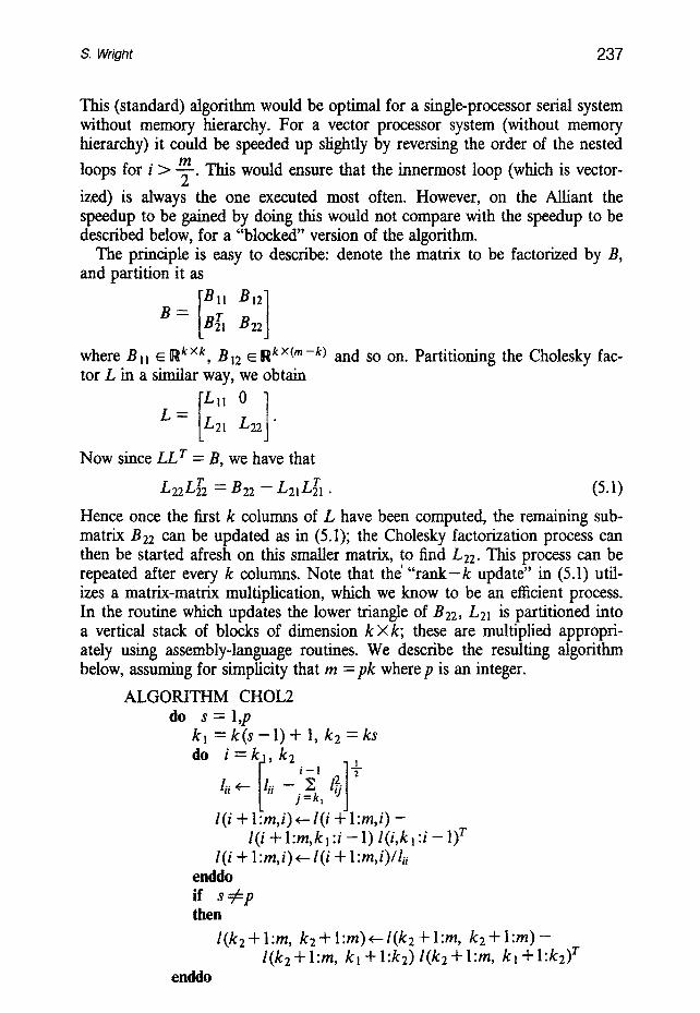
This (standard) algorithm would be optimal for a single-processor serial system without memory hierarchy. For a vector processor system (without memory hierarchy) it could be speeded up slightly by reversing the order of the nested

m loops for i > -~-. This would ensure that the innermost loop (which is vector-

ized) is always the one executed most often. However, on the Alliant the speedup to be gained by doing this would not compare with the speedup to be described below, for a "blocked" version of the algorithm.

The principle is easy to describe: denote the matrix to be factorized by B, and partition it as

Bll B 2]

where B!1 ~ R k×k, Bx2 ~ R k×(m-k) and so on. Partitioning the Cholesky factor L in a similar way, we obtain 0 ]

L = L 2 1 L 2 2 "

Now since LLT" = B, we have that

L22LT2 " - B 2 2 - LEILTI . (5.1)

Hence once the first k columns of L have been computed, the remaining submatrix B22 can be updated as in (5.1); the Cholesky factorization process can then be started afresh on this smaller matrix, to find LEE. This process can be repeated after every k columns. Note that the' " r a n k - k update" in (5.1) util- izes a matrix-matrix multiplication, which we know to be an efficient process. In the routine which updates the lower triangle of B22, LEl is partitioned into a vertical stack of blocks of dimension k ×k; these are multiplied appropri- ately using assembly-language routines. We describe the resulting algorithm below, assuming for simplicity that m = pk where p is an integer.

ALGORITHM CHOL2 do s = l,p

kl = k ( s - 1 ) + 1, k2 = k s = k ,k2

i - I T

Ilia..- - - ~, j = k l

l(i + l : m , i ) ~ l ( i + 1 :m,i) - l(i + l:m, kl :i - 1) l(i, kl :i - 1) r

l(i + 1 :m,i) ~ l(i + 1 :m,i)/lii enddo if s =/=p then

l(k2 + l:m, k2 + l : m ) ~ l ( k 2 + l:m, k 2 + l : m ) - l(k2 + l:m, kl + l:k2) l(k2 + l:m, kl + l:k2) r

enddo


Here, the notation

l(]'i:j2, j3:j4) refers to the submatrix of L formed by rows j l through jz, and columns j3 through ja. Note that only the lower submatrix of L need be updated in the last step of Algorithm CHOL2. Also, CHOL1 can be recovered from CHOL2 by setting k = m.

An alternative "fast" implementation can be achieved by delaying the update of each block of columns until just before that block is to be factorized. That is, before factorizing columns kl through k2, a rank - k l - 1 update is applied to the block. The resulting algorithm can be described as follows:

ALGORITHM CHOL3 do s = l,p

kl = k ( s - 1 ) + 1, k2 = k s if s > l then

l (kl :m, k l :k2)*--l(kl :m, k l :k2) - l (k l :m, l : k l - l ) l (k l :k2, l :kl--1) r

do i - k~ k2 ] 4 / i - - I

l(i + l : m , i ) ~ l ( i + l:m,i) -- l(i + l:m, kl :i - 1) l(i, k l :i - 1) r l(i + l:m,i) ,-- l(i + l:m,i)/lii

enddo enddo

Four versions of the algorithms above were tested. The first version is simply a FORTRAN implementation of Algorithm CHOL1, compiled under full optimization to run concurrently on all eight processors. The second version is identical, except that the level 2 BLAS routine 'DMXV is called to perform the matrix-vector multiplication inherent in each iteration of CHOL1. (The kernel of DMXV is coded in assembly language.) Comparative results for these two versions are given in Table 5.1. A speedup of approximately three is noted in the second version.

S. Wright 239

m

CHOLI (FORTRAN) CHOL1 with DMXV

time(s) Mflops times(s) Mflops 500 8.97 4.6 2.59 16.1

1000 62.33 5.3 19.78 16.9 1500 172.3 6.5 62.00 18.1

TABLE 5.1 Performance of Algorithm CHOL1; fully-optimized FOR- TRAN implementation vs implementation via an assembly-language BLAS routines.

The third version is a FORTRAN implementation of CHOL2 which again called DMXV to do the matrix-vector multiplication, and, in addition, repeat- edly uses the level 3 BLAS routine DTMXM to perform the r a n k - k update at the end of each major iteration. The fourth version is a FORTRAN implementation of CHOL3, which calls the same BLAS routines but in a different order. Test results are given in Tables 5.2 to 5.4. To ensure a fair comparison, Mflop

1 3 rates are calculated using a uniform operation count of y m throughout, even

though the ~ctual operation counts for CHOL2 and CHOL3 are stghtly greater (by 2ink). The timings for the second version of Algorithm CHOLI

are added to these tables for comparison.

CHOL2 CHOL3 k time(s) Mflops time(s) Mflops

8 2.69 15.5 1.82 22.9 16 1.95 21.4 1.69 24.7 32 1.69 24.7 1.69 24.7 64 1.79 23.3 1.74 24.0

128 2.30 18.1 CHOL1 2.59 16.1

TABLE 5.2 Performance of Algorithm CHOL2 and CHOL3 for m = 500, for different blocksizes k.


CHOL2 CHOL3 k time(s) Mflops time(s) Mflops

16 17.24 19.3 11.84 28.1 32 11.66 28.6 11.67 28.6 64 11.43 29.2 12.15 27.4

128 13.28 25.1 CHOL1 19.78 16.9

TABLE 5.3 Performance of Algorithm CHOL2 and CHOL3 rn = 1000, for different blocksizes k.

for

CHOL2 k time(s) Mflops

16 47.99 23.4 32 37.28 30.2 64 35.16 32.0

128 39.90 28.2 CHOL1 62.00 18.1

CHOL3 time(s) Mflops 37.41 30.1 35.50 31.7 35.87 31.4

TABLE 5.4 Performance of Algorithm CHOL2 and CHOL3 for m = 1500, for different blocksizes k.

It can be seen from these tables that the best times achieved by these two algorithms are very similar; CHOL3 is perhaps preferable because it is less sensi- tive to the choice of k. The speedup gained by these two methods relative to CHOL1 increases, approaching a factor of 2 for the largest test problem.

Finally, we note that the best Mflop rates attained by Algorithms CHOL2 and CHOL3 compare well with the 38 Mflop peak rate for level 3 BLAS matrix-multiply routines. Because there is unavoidably a certain amount of matrix-vector computation in any Cholesky algorithm, it is doubtful that a much closer approach to this peak rate could be made.

6. NUMERICAL RESULTS FOR ALGO~TrIM QPE We now present timing results for the Algorithm QPE of section 3. Again, three implementations are discussed. The "benchmark" implementation (referred to as QPEBEN) uses the algorithm QR1 together with (4.5) from section 4 to perform step 1, and the Algorithm CHOL1 (with BLAS) to perform step 4. These have been discussed in the previous two sections. The "blocked" implementation of QPE differs only in that the faster algorithms from the last two sections (CHOL2 and QR2 + (4.6)) are used for steps 4 and 1, respectively. The choices of blocksize for QR2 are the same as in Table 4.1, while the following algorithm was used to determine the blocksize for CHOL2:

S. Wright 241

if m < 64 then k = 1 else if 64 ~< m ~< 256 then k = m/8 else k = 32.

All implementations use double-precision arithmetic. Table 6.1 shows the execution time for the benchmark implementation QPE-

BEN, for randomly-generated test problems of varying size. Results for vectorized implementation on one processor, and fuUy-optimized implementation on all eight processors are given. The correctness of the results is checked using the first-order conditions (3.7) and (3.8). As shown in Table 6.1, almost all of the execution time is spent in steps (1) and (4) of the algorithm, with step (1) dominating except when t is small compared to n. "Parallel" speedup behaviour is similar to that observed in Table 4.2.

Table 6.2 shows the results for the "blocked" implementation of QPE. Here step (1) is not quite so dominant, reflecting the fact that it was possible to achieve greater speedup in this step than in step (4).

Table 6.3 shows the "block" speedup obtained on these seven test problems, showing that the best speedup was obtained on the larger test problems, where t is comparable in magnitude to n.

1 Processor 8 Processors "Parallel" Proportion Proportion n t time(s) time(s) speed up in (1) in (5) 100 80 1.61 .61 2.6 .92 .O1 500 400 186.66 40.71 4.6 .99 .001 750 500 539.94 110.63 4.9 .99 .003 500 250 128.91 27.73 4.6. .98 .01

1000 500 1012.30 197.95 5.1 .98 .01 500 50 37.68 7.59 5.0 .74 .24

1000 100 290.53 54.12 5.4 .73 .26

TABLE 6.1 Execution Times for benchmark implementation QPEBEN, with proportion of time spent in steps 1 and 5.


Proportion Proportion n t Total Time in (1) in (5) 100 80 .41 .87 .02 500 400 14.16 .98 .003 750 500 38.20 .98 .007 500 250 10.50 .95 .03

1000 500 69.24 .97 .02 500 50 3.74 .63 .32

1000 100 23.94 .63 .34

TABLE 6.2 Execution times for "blocked" version of QPE, with proportion of time spent in steps 1 and 5.

"block" n t Speedup 100 80 1.5 500 400 2.9 750 500 2.9 500 250 2.6

1000 500 2.9 500 50 2.0

1000 100 2.3

TABLE 6.3 Speedup of blocked implementation over benchmark implementation of QPE

7. CONCLUSION We have presented some techniques for speeding up the null-space method for equality-constrained quadratic programming on a parallel machine with memory hierarchy, such as the Alliant FX/8. Test results on a set of problems which fit comfortably into the main memory of that machine showed that "block" speedups approaching 3 were attainable. The techniques therefore seem to be suitable for small to medium-sized dense problems.

As pointed out in the introduction, the equality-constrained quadratic programming problem is a basic component of many algorithms for constrained optimization. In future we will report on enhancements to these algorithms, both by using the techniques of this paper, and other techniques associated with management of the active set and evaluation of the objective and constraint functions.

S. Wright 243

REFERENCES [1] Alliant FORTRAN Library Documentation, Center for Supercomputing

Research and Development, University of Illinois at Urbana-Champaign, June 1986.

[2] C. BISCHOF and C. VAN LOAN, The WY representation for products of Householder matrices, SIAM J. Sci. Stat. Comp. 8 (1987) s2-s13.

[3] A.R. Co~¢N and N.I.M. GOULD, On the location of directions of infinite descent for nonlinear programming algorithms, SIAM J. Numer. Anal. 21 (1984) 1162-1179.

[4] R. FLETCHER, Practical methods of optimization. Volume 2: Constrained optimization, (John Wiley and Sons, 1981.)

[5] P.E. GILL, W. MURRAY and M.H. WRIGHT, Practical optimization, (Academic Press, 1981.)

[6] W.J. HAgROD, Solution of the linear least squares problem on the Alliant FX/8, Technical Report, Center for Supercomputing Research and Development, University of Illinois, 1986.

[7] W. JALBY and U. MEIER, Optimizing matrix operations on a parallel multiprocessor with a memory hierarchy, Technical Report, Center for Super- computing Research and Development, University of Illinois, 1986.

A fast algorithm for equality-constrained quadratic programming on the alliant FX/8

Documents

Transcript of A fast algorithm for equality-constrained quadratic programming on the alliant FX/8