A FACTOR MODEL OF THE TERM STRUCTURE OF … · a factor model of the term structure of interest...
31
‹ Latvijas Banka, 2006 The source is to be indicated when reproduced. Fragments of the painting by have been used in the design. White Move (2005) Juta Policja and Mareks Gureckis The views expressed in this publication are those of the authors, employees of the Monetary Policy Department of the Bank of Latvia. The authors assume responsibility for any errors and omissions. A FACTOR MODEL OF THE TERM STRUCTURE OF INTEREST RATES AND RISK PREMIUM ESTIMATION FOR LATVIA'S MONEY MARKET VIKTORS AJEVSKIS KRISTÎNE VÎTOLA WORKING ISBN 9984–676–83–8 1 2006 PAPER
Transcript of A FACTOR MODEL OF THE TERM STRUCTURE OF … · a factor model of the term structure of interest...

lsaquo Latvijas Banka 2006
The source is to be indicated when reproduced
Fragments of the painting by have been used in the designWhite Move (2005) Juta Policja and Mareks Gureckis
The views expressed in this publication are those of the authors employees of the Monetary Policy Department of theBank of Latvia The authors assume responsibility for any errors and omissions
A FACTOR MODEL OF THE TERM STRUCTURE OF INTEREST RATES
AND RISK PREMIUM ESTIMATION FOR LATVIAS MONEY MARKET
VIKTORS AJEVSKIS
KRISTIcircNE VIcircTOLA
W O R K I N G
ISBN 9984ndash676ndash83ndash8
1 2006
P A P E R
A FACTOR MODEL OF THE TERM STRUCTURE OF INTEREST RATES AND RISK PREMIUM ESTIMATION FOR LATVIAS MONEY MARKET
1
CONTENTS
Abstract 2 Introduction 3 1 Factor Models of the Term Structure of Interest Rates 5 2 Empirical Results 10 21 Data 10 22 Model Estimation 10 23 The Risk Premium 11 24 Explanation of Risk Premium Behaviour 14 Conclusion 16 Appendices 17 Bibliography 29
ABBREVIATIONS CB ndash central bank EONIA ndash Euro Overnight Index Average GDP ndash gross domestic product LIBOR ndash London Interbank Offered Rate RIGIBID ndash Riga Interbank Bid Rate RIGIBOR ndash Riga Interbank Offered Rate SDR ndash Special Drawing Rights VAR ndash vector autoregression
A FACTOR MODEL OF THE TERM STRUCTURE OF INTEREST RATES AND RISK PREMIUM ESTIMATION FOR LATVIAS MONEY MARKET
2
ABSTRACT The paper presents the analysis of risk premium of the interest rate term structure for the Latvian money market On the back of the approach used by F Diebold G Rudebusch and B Aruoba it has been assumed that the coefficients of the NelsonndashSiegel model are unobservable therefore the model of this research paper has been estimated using the Kalman filter The risk premium behaviour has been obtained for interest rates of different maturities and forecasting horizons between May 2000 and July 2005 The results obtained indicate that the amount of the risk premium was significant and its volatility substantial between 2000 and 2002 In post-2002 period its behaviour gradually stabilised and was marked by a downward trend after 2004 Key words term structure of interest rates risk premium the NelsonndashSiegel model the Kalman filter JEL classification codes C32 D84 E43 E47 G10
A FACTOR MODEL OF THE TERM STRUCTURE OF INTEREST RATES AND RISK PREMIUM ESTIMATION FOR LATVIAS MONEY MARKET
3
INTRODUCTION Information captured in the prices of financial assets gives signals to CBs about the expectations of market participants regarding such fundamentals as the future economic activity inflation and short-term interest rate dynamics The analysis of these expectations plays a significant role for the future policy process Aiming for its core objective of price stability the Eurosystem as an example consistently adheres to the two-pillar strategy when implementing its monetary policy and the financial asset prices are important for it as the second pillar indicator(19) Financial asset prices are a reflection of market participants expectations because the former are in fact forward-looking The present asset prices are determined by discounting expected future payment flows Two factors affect the discount rate used in the financial asset assessment 1) compensation for consumption postponed to the future and not used at the current point in time and 2) compensation for the risk associated with the future payment flow uncertainties In the assessment of a financial asset the investor shall be able to predict the future payment flows and the discount rates with risk premiums included that are applicable to these flows The price of fixed income financial instruments is determined by interest rates to be used in discounting the respective payment flows The interest rates in turn are dependent upon the expectations of the fundamental macroeconomic variables like inflation and the real interest rates as well as upon the compensation for risks related to uncertainty of the respective expectations Information about financial market participants expectations regarding future interest rates is particularly significant for CBs because it helps them foresee if a particular decision will surprise market participants and what their short-term reaction to it could be The official future interest rate expectations figure prominent also when the current monetary policy stance is formulated Changes in long-term interest rates that primarily depend on the expected official future interest rates affect many participants of the financial market Therefore aiming for the assessment and control over current shifts in the monetary situation CBs need to have some understanding about market participants expectations about the official future interest rates Forward rates are the most widely used measure of interest rate expectations They are the implied future interest rates incorporated in the present interest rates for different maturities Provided that uncertainties associated with future interest rates were absent forward interest rates would be equal to the expected future interest rates However the future interest rates are not known for sure In order to hold this interest rate risk the investors who want to avoid the risk would demand a risk premium In such a way in equilibrium this will drive a wedge ndash the risk premium ndash between the forward rate and the expected short-term interest rate In addition longer future horizons are related to a more pronounced uncertainty regarding possible interest rate movements hence the respective risk premium is likely to increase with maturity Consequently the longer the time horizon the larger becomes the difference between the forward rate and the expected rate
A FACTOR MODEL OF THE TERM STRUCTURE OF INTEREST RATES AND RISK PREMIUM ESTIMATION FOR LATVIAS MONEY MARKET
4
In this study the risk premium is defined as the difference between the forward rate and the expected future interest rate pr iEf t
To estimate the expected future interest rate the procedure proposed by F Diebold and C Li was used(4) These authors proved that a relatively precise forecast of the term structure of interest rates can be derived from autoregressive models for factors corresponding to the level slope and curvature of the yield curve Basing on the approach of F Diebold G Rudebusch and B Aruoba (6) the study assumes that these unobservable factors correspond to the NelsonndashSiegel model coefficients that are estimated and predicted in this study using the Kalman filter(13) The authors of this study have opted for the Kalman filter because it has certain advantages over other econometric methods Due to the ongoing transition of Latvias economy a great number of economic variables are not stationary As is known the Kalman filter provides an opportunity to work with non-stationary variables Moreover economic variables are affected by a number of factors eg the investment and political climate that cannot be accurately estimated and the Kalman filter allows for the estimation of economic variables and factors that are changing over time Chapter 1 defines some basic theoretical concepts that are needed for further analysis and builds the theoretical framework for the factor model of the term structure of interest rates Chapter 2 deals with the factor model on the back of Latvias data Section 21 reviews the selected data sample Section 22 analyses the estimates obtained by the Kalman filter Section 23 presents the results of the estimated risk premium Section 24 describes the empirical results The most important effects of the study are summed up in the Conclusion Appendix 1 presents the theoretical framework of the Kalman filter Appendices 2ndash5 furnish the risk premium dynamics for 1- 3- 6- and 12-month interest rates at different forecasting horizons while Appendix 6 sums up mean premiums and standard deviations for 1- 3- 6- and 12-month interest rates
A FACTOR MODEL OF THE TERM STRUCTURE OF INTEREST RATES AND RISK PREMIUM ESTIMATION FOR LATVIAS MONEY MARKET
5
1 FACTOR MODELS OF THE TERM STRUCTURE OF INTEREST RATES The introductory part of the Chapter defines and describes the basic theoretical concepts i(tT) denotes the nominal spot interest rate ie the yield to maturity of a zero-coupon bond bought at time t with T gt t maturity date Assuming that no-arbitrage restriction is imposed the nominal implied forward interest rate at time t with the delivery term τ and maturity at T can be defined as follows (17)
)()(1)(
)()()()(
ttiT
ttitTTtiTtf
[11]
The forward rate premium is calculated as the difference between the forward interest rate and the expected future interest rate pr )()()( TiETtfTt t [12]
where Et is the conditional mathematical expectations operator for information available at time t Taking into account that the forward rate at each time t can be calculated using equation [11] premium determination should rest upon the estimation of )( TiEt Provided that
an appropriate model is used this term can be defined as a modelled forecast for the respective interest rate Obviously the forecasts of different time horizons τ ndash t and those of interest rates on different maturities T ndash τ must be interrelated Indeed this model should capture the entire term structure of interest rates As there are considerably fewer sources of systematic risk than there are tradable financial instruments all price information of tradable interest-rate-based financial instruments can be accumulated in a few variables or factors(15 16) Consequently term structure factor models of interest rates use structures with a small number of interest rate factors and the associated factor loadings that relate interest rates on different maturities to these factors Factor structures ensure useful data compression and simultaneously the so-called parsimony principle A number of approaches to constructing the interest rate factors and loadings of these factors are presented in the literature The factors may be the first principal components that are orthogonal to each other by definition while the loadings may be relatively unrestricted(15 16) The first three principal components are usually correlated to the level slope and curvature of the yield curve Another approach widely employed by practitioners and CBs is the NelsonndashSiegel model (introduced in the work of C Nelson and A Siegel (17)) Factor loadings in the NelsonndashSiegel model have economically plausible restrictions the forward rates are always positive and with the term to maturity increasing the discount function approaches zero A no-arbitrage dynamic latent factor model is the third approach The most general subclass of latent factor models postulates a linear or affine functional relationship of latent factors with interest rates and restrictions on the factor loadings that rule out arbitrage strategies involving interest rate instruments
A FACTOR MODEL OF THE TERM STRUCTURE OF INTEREST RATES AND RISK PREMIUM ESTIMATION FOR LATVIAS MONEY MARKET
6
According to the factor model approach a large set of yields of various maturities is expressed as a function of a small number of unobserved factors The set of yields is denoted as y(τ) where τ is the term to maturity CBs use widely the Nelson-Siegel (17) curve to represent the cross-section yield data
eee
y11
)( 321 [13]
where β1 β2 β3 and λ are the parameters Parameter λ captures velocity at which exponential terms decrease The study assumes it to be a constant because this assumption considerably reduces volatility of parameters it rendering their behaviour
more predictable Parameters β1t β2t and β3t are interpreted as three latent (unobservable) factors(6) Factor loading of β1t is equal to 1 ie as it remains unchanged thus
t1 can be considered a long-term factor Factor loading for β2t is )1( e
This
function equal to 1 if 0 and monotonically decreasing to 0 can be considered a
short-term factor The loading of β3t is
ee )1(
it is the function equal to 0 if
0 (ie it is not a short-term factor) growing to its maximum at
81
and
afterward reversing to 0 (ie it is not a long-term factor) that hence can be considered a medium-term factor Chart 11 presents the given factor loadings under the condition that 2
The long-term short-term and medium-term factor can be interpreted as the level slope and curvature of the yield curve respectively For example the long-term factor t1
describes the level of the yield curve In addition the relation tyy 1)(lim)(
can be derived from equation [13] An increase in t1 would cause a rise by the same
amount in all yields )(y and simultaneously push up the level of the yield curve Several authors eg J A Frankel and C Lown (11) define the slope of the curve as
)0()( tt yy which according to formula [13] is t2 In such a way the short-term
factor t2 determines the slope of the yield curve Due to an increase in t2 the short-
A FACTOR MODEL OF THE TERM STRUCTURE OF INTEREST RATES AND RISK PREMIUM ESTIMATION FOR LATVIAS MONEY MARKET
7
term rates grow faster than the long-term rates because loading )1( te
which is
multiplied by t2 at small values would be close to 1 but at large values it would
be close to 0 which in turn causes shifts in the slope of the yield curve An increase in factor t3 on the other hand has little effect on the rise of short-term
and long-term interest rates because factor loading
t
t
ee )1(
would be close to
0 at both large and small values of and would more affect the growth of the medium-term interest rates (with a maximum growth in interest rates corresponding to maturity
81) thus increasing the curvature of the yield curve
As has been proved by F Diebold and C Li (4) the NelsonndashSiegel curve can be represented as a dynamic latent factor model with β1 β2 and β3 as time-varying factors of level slope and curvature the terms multiplied by these factors are factor loadings Thus the model can be represented as follows
ee
Ce
SLy tttt
11)( [14]
where Lt St and Ct are the time-varying variables β1 β2 and β3 This approach will be further supported by empirical estimates If the dynamics of Lt St and Ct follows a vector autoregressive process of the first order this model forms a state-space system The transition equation governing the dynamics of the state vector is [15]
where t = 1 hellip T is the time series length in the sample The equation that relates a set of N yields to the three unobservable factors can be written
)(
)(
)(
111
111
111
)(
)(
)(
2
1
22
11
2
1
2
22
1
11
Nt
t
t
t
t
t
NN
Nt
t
t
C
S
L
eee
eee
eee
y
y
y
N
NN
[16]
Using generally accepted vector and matrix notations the given state-space system can be written
)(
)(
)(
1
1
1
333231
232221
131211
C
S
L
C
S
L
aaa
aaa
aaa
C
S
L
t
t
t
t
t
t
C
S
L
t
t
t
A FACTOR MODEL OF THE TERM STRUCTURE OF INTEREST RATES AND RISK PREMIUM ESTIMATION FOR LATVIAS MONEY MARKET
8
ttt A 1 [17]
ttty [18]
where vector )( tttt CSL
To achieve the linear least squares optimality of the Kalman filter we assume a condition that the white noise transition and measurement disturbances are orthogonal both mutually and relative to the initial state
Q
HWN
t
t
0
0
0
0~ [19]
0)( 0 tE [110]
0)( 0 tE [111]
The analysis is dominated by the assumption that H and Q matrices are diagonal The assumption regarding a diagonal Q matrix which implies mutually uncorrelated deviations of yields of various maturities from the yield curve is quite common Despite the fact that F Diebold G Rudebusch and B Aruoba did not impose any restrictions on matrix H non-diagonal matrix elements turned out to be insignificant(6) Therefore for computation simplicity this paper deals only with the diagonal type of matrix H Overall the state-space approach ensures an effective framework for the analysis and estimation of dynamic models The inference that the NelsonndashSiegel model can easily be transformed into a state-space model is particularly useful because in this case the Kalman filter produces estimates of the maximum likelihood along with optimally filtered and smoothed estimates of the model factors Moreover in this paper preference is given to the one-step Kalman filter method rather than the two-step DieboldndashLi approach because according to the standard theory simultaneous estimation of all parameters results in correct inferences By contrast the two-step approach has a drawback the uncertainty of parameter estimation and signal extraction via the first step is not accounted in the second step computations Furthermore the state-space approach raises a possibility of future extensions eg existence of heteroskedasticity shortage of data etc albeit the present paper does not take on the task of dealing with such extensions It is useful to compare the approach used in this paper with those proposed by other authors An unrestricted VAR estimated for a set of yields is a very general (linear) model This model has a potential drawback of its results being possibly dependent on the particular selected set of yields The aforementioned factor representation can aggregate information from a large set of yields Another factor model ranking among the simplest ones is VAR estimated with the principal components1 which have been formed from a large set of yields This approach imposes a restriction on factors to be mutually orthogonal yet it does not fully restrict factor loadings However the model used in this paper potentially allows for factor correlation but restricts factor loadings imposing limits on the set of admissible yield curves For instance the NelsonndashSiegel
1 VAR term structur analysis can be found in the works of eg C Evans and D Marshall (9 10)
A FACTOR MODEL OF THE TERM STRUCTURE OF INTEREST RATES AND RISK PREMIUM ESTIMATION FOR LATVIAS MONEY MARKET
9
model guarantees positive forward interest rates for all time periods and also as maturities increase the converging of the discount function toward 0 Such economically-founded restrictions are likely to support the analysis of the yield curve dynamics It is also possible to introduce alternative restrictions of which the non-arbitrage restriction is imposed most often It ensures consistency in interest rate adjustments of the yield curve over time Nevertheless the evidence on the extent to what these restrictions affect the results is quite varied2
2 Works of eg A Ang and M Piazessi (1) as well as G Duffee (7) can be used for comparison
A FACTOR MODEL OF THE TERM STRUCTURE OF INTEREST RATES AND RISK PREMIUM ESTIMATION FOR LATVIAS MONEY MARKET
10
2 EMPIRICAL RESULTS 21 Data
Arithmetic means of 1- 3- 6- 9- and 12-month RIGIBID and RIGIBOR have been used to estimate the model in this study Interest rates of shorter maturities are not analysed because their variance (particularly that of overnight rates) is excessively pronounced at the end of the reserve maintenance period Monthly data for the period from May 2000 to July 2005 have been used3 Interest rates have been computed as daily arithmetic means of the respective month
22 Model Estimation The model of this paper forms a state-space system where the VAR(1) transition equation describes the dynamics of the vector of latent state variables with the linear equation linking the observed yields with state vector In contrast to F Diebold G Rudebusch and B Aruoba (6) this study makes use of independent autoregressive first order specifications for each state variable ie all non-diagonal elements of matrix A are equal to zero This approach allows for a considerable reduction in the number of coefficients to be estimated taking into account the condition of a rather short time series In the research of F Diebold G Rudebusch and B Aruoba all off-diagonal coefficients are insignificant therefore it justifies the specification selection for the present study In addition the work of F Diebold and C Li (4) deals with the autoregressive specification of Lt Ct St as well yet the estimation of the coefficients instead of being carried out using the Kalman filter (as in the present study due to its advantages) is based on the two-step method Several model parameters are to be estimated The (3 x 3) dimensional transition diagonal matrix A comprises three free parameters the (3 x 1) dimensional constant vector μ has three free parameters and the measurement matrix Λ comprises one free parameter λ In addition the transition and disturbance covariance matrix Q contains three free parameters (one disturbance variance for each of the three latent factors level slope and curvature) while the measurement disturbance covariance matrix H has five free parameters (one disturbance variance for each of the five yields) Consequently overall 15 parameters are to be estimated via optimisation and it is a complex numerical exercise For computing optimal yield forecasts and the related errors the Kalman filter has been applied to this configuration of parameters afterwards the Gaussian likelihood function has been estimated for the model using the prediction-error decomposition of the likelihood The theoretical frame of the Kalman filter is detailed in Appendix 1 For initialisation of the Kalman filter the values of the state variables are used applying the least square method and cross-sectional data at time t = 1 (the first observation in the time series) Table 221 presents the results of the estimated model Autoregressive coefficients Lt Ct and St point to a highly persistent dynamics (099 088 and 085 respectively) The values thus obtained are extremely close to those in F Diebold G Rudebusch and
3 As of May 2000 the Bank of Latvia started the computation of 9- (for internal use) and 12-month RIGIBID and RIGIBOR therefore for the purpose of a larger sample the period starting with May 2000 has been selected
A FACTOR MODEL OF THE TERM STRUCTURE OF INTEREST RATES AND RISK PREMIUM ESTIMATION FOR LATVIAS MONEY MARKET
11
B Aruoba (the coefficients are 099 094 and 084 respectively) As in the study of the above authors when moving from Lt to St to Ct the transition shock volatility increases Though all the constants are insignificant they remain in the specification of this paper to rule out the possibility of unstable estimates
Table 221 Model Parameter Estimates
L S C μL μS μC σL σS σC
0994 (0013)
0890 (0046)
0850 (0098)
ndash0054 (0087)
ndash0078 (0091)
ndash0002 (0121)
0011 (0015)
0132 (0021)
0271 (0077)
Note Standard errors of coefficients are given in brackets
23 The Risk Premium In the study the risk premium is defined as the difference between the forward rate f and the expected future interest rate of the respective maturity )( TiEt
pr )()()( TiETtfTt t
where )( TiEt is derived using
)(
)()(
)(
1
)(
1)( T
T
t
T
ttt eT
eC
T
eSLTiE
where )()( ttttt ECSL is the forecast of state variables )( t steps
ahead under the condition that the initial value of tt is the state variable values filtered
at time t The filtered values of state variables are used also in the calculations of forward rates
)()(1)(
)()()()(
ttiT
ttitTTtiTtf
where
)(
)()(
)(
1
)(
1)( t
t
tt
t
tttt et
eC
t
eSLti is the theoretical
interest rate value consistent with the NelsonndashSiegel model at time t Chart 231 shows risk premium pr(t12) on 1-month interest rate for one month forecasting horizon It should be noted that the risk premium defined in this study is correct if the estimated expectation measure is correct as a forecast obtained with the help of the Kalman filter Chart 231 demonstrates that up to 2002 the volatility of risk premium was substantial then it stabilised and after that its decline from 36 basis points in October 2004 to 16 basis points in July 2005 was recorded At the close of 2004 the said decline in risk premium was associated with the market participants expectations for repegging of the lats from the SDR basket of currencies to the euro which implied a smaller exchange risk The risk premium continued to shrink also at the beginning of 2005 which was likely to be associated with the ongoing convergence Appendix 2 shows the dynamics of 1-month interest rate risk premium for the horizon of 2ndash12 months Some points in time with negative risk premiums notwithstanding the premium remains positive on average over the entire reporting period Negative risk premiums
A FACTOR MODEL OF THE TERM STRUCTURE OF INTEREST RATES AND RISK PREMIUM ESTIMATION FOR LATVIAS MONEY MARKET
12
may imply the presence of a number of expectation errors The premium values for forecasting horizons exceeding 4 months are only positive Appendices 3 4 and 5 highlight a similar behaviour for 3- 6- and 12-month interest rate premiums
For the purpose of estimating the average premium of the reviewed period the arithmetic mean premium of the period and its standard deviation for 1- 3- 6- and 12-month interest rates have been computed Chart 232 and 233 show arithmetic mean risk premiums and their standard deviations for 1ndash12 month forecasting horizon The premiums are positive according to the prediction and with the forecasting horizon growing they increase The longer the horizon the larger premium is demanded by market participants By contrast standard errors display a tendency to increase in the period up to six month horizon after which they decline steadily The tables of Appendix 6 report mean risk premiums on 3- 6- and 12-month interest rates and their standard deviations Data in Appendix 6 lead to an inference that the behaviour of 3- 6- and 12-month interest rate premiums and standard deviations is similar to the behaviour of 1-month interest rates
Premiums with the same forecasting horizon but different term to maturity display a peculiar tendency of behaviour With the interest rate term increasing the risk premium decreases Chart 234 demonstrates the behaviour of 1- 3- 6- and 12-month risk premiums for one month forecasting horizon The Chart shows that over a longer term the risk premium decreases A similar relation is observed also for 2ndash12 month forecasting horizon The theoretical reasoning for the behaviour of the risk premium within this model is provided in Chapter 24
A FACTOR MODEL OF THE TERM STRUCTURE OF INTEREST RATES AND RISK PREMIUM ESTIMATION FOR LATVIAS MONEY MARKET
13
Table 231 presents the comparison of Latvian interest rate risk premiums with those of other countries and their evaluation in different sources The analysis of the data leads to a conclusion that at present the interest rate risk premiums in Latvia are higher than in the developed countries The ongoing convergence is likely to bring interest rate risk premiums in lats closer to those of the euro area
Table 231 Risk Premiums in Latvia and Other Countries (1-month interest rate risk premiums for different forecasting horizons in basis points)
1 month 3 months 6 months 9 months
Latvia1 19 52 88 1161-month LIBOR Germany (December 1989ndashDecember 1998)2 5 10 15 27
EONIA swap rates
January 1999ndashSeptember 20012 0 2 6 10
January 1999ndashJune 20022 1 2 4 13
Germany (1972ndash1998)3 0ndash5 5ndash10 20ndash25 25ndash35
Canada (1988ndash1998)4 6 29 58 100 1 Results of this paper 2 (8) 3 (2) 4 (13)
A FACTOR MODEL OF THE TERM STRUCTURE OF INTEREST RATES AND RISK PREMIUM ESTIMATION FOR LATVIAS MONEY MARKET
14
24 Explanation of Risk Premium Behaviour
This Chapter attempts to explain theoretically the empirical behaviour of the above-referred risk premium within the framework of the researched model In compliance with equation [12] above pr )()()( TiETtfTt t [21]
For simplicity we shall replace equation [11] with the following definition of the forward rate
)(
)()()()(
T
ttitTTtiTtf [22]
which corresponds to a continuously compounded rate The substitution of elements from equation [14] into [22] instead of i(t τ) and i(t T) gives
)()(
)()()()(
)()()(
)( tTttTt
t
tTt
tt etTetT
eeC
T
eeSLTtf
[23] The interest rate forecast from equation [14] is
CEe
T
eSE
T
eLETiE t
TT
t
T
tt)(
)()(
)(
1
)(
1)( [24]
where Et(Lτ) Et(Sτ) and Et(Cτ) are forecasts of the respective factors at time t for the future period τ Accounting for the factor dynamics subjection to the first order autoregressive process let us produce the following factor forecast equations
11
1111
1111111 1
11
a
aLaaaLaLE
t
Lttt
Ltt
t
[25]
22
2222
1222222 1
11
a
aSaaaSaSE
t
Sttt
Stt
t
[26]
33
3333 1
1
a
aCaSE
t
Ctt
t
[27]
Equations [21] and [23]ndash[27] give the following risk premium
A FACTOR MODEL OF THE TERM STRUCTURE OF INTEREST RATES AND RISK PREMIUM ESTIMATION FOR LATVIAS MONEY MARKET
15
pr
)()()()(
)()(
T
eeSLTiETtfTt
tTt
ttt
11
1111
)()()()(
1
1)(
)( a
aLaetTet
T
eeC
t
LtttTt
tTt
t
33
3333
)()(
22
2222
)(
1
1
)(
1
1
1
)(
1
a
aCae
T
e
a
aSa
T
e t
CttT
Tt
Stt
T
[28] Chart 241 shows the risk premium from equation [28] as the function of interest rate maturity (T ndash t) at the forecasting horizon τ ndash t = 1 month Factor values of this risk premium Lt = 2756 St = ndash0482 Ct = 0048 and coefficients aii and μj correspond to the Kalman filter estimates of July 2005 ie the last sample observation The Chart discloses that at the given parameter values the function is declining if T ndash t is growing and this is in support of the empirical facts referred to in the previous Chapter
When we fix the interest rate term T ndash τ = 1 month for equation [28] with these parameter values and change the forecasting horizon we obtain the risk premium curve which depending on the horizon is presented in Chart 242 The Chart shows that when the forecasting horizon increases the risk premium grows It confirms the empirical facts and heuristic assumptions from Chapter 23 about investors demanding higher risk premiums for larger uncertainty related to investments at a more distant point in time
A FACTOR MODEL OF THE TERM STRUCTURE OF INTEREST RATES AND RISK PREMIUM ESTIMATION FOR LATVIAS MONEY MARKET
16
CONCLUSION The paper presents the analysis of risk premium of the interest rate term structure for the Latvian money market The risk premium has been defined as the difference between the forward interest rate and the expected future interest rate of the respective maturity The interest rate term structure is assessed consistently with the NelsonndashSiegel model On the back of the approach used by F Diebold G Rudebusch and B Aruoba it has been assumed that the coefficients of the NelsonndashSiegel model are unobservable therefore the model of this research paper has been estimated using the Kalman filter RIGIBID and RIGIBOR interest rates of the Latvian money market have been used as the observable variables The expected future interest rate has been computed as the Kalman filter forecast n periods ahead The risk premium behaviour has been obtained for interest rates of different maturities and forecasting horizons between May 2000 and July 2005 The results obtained indicate that the amount of the risk premium was significant and its volatility substantial between 2000 and 2002 In post-2002 period its behaviour gradually stabilised and was marked by a downward trend after 2004 This is in support of the assumption that with the forecasting horizon increasing the risk premium grows while with the expansion of maturity it becomes smaller These facts have been explained theoretically in the paper on the basis of the models mathematical structure The risk premium estimation becomes more complicated when the market participants expectations embedded in the financial market data are to be analysed The respective analysis carried out within this research has proposed an additional instrument for a CB to timely identify the market participants expectations regarding interest rates in the future and to learn about their confidence in the conducted monetary policy Nevertheless the employment of such instruments as money market RIGIBID and RIGIBOR restricts the forecasting horizon to one year In order to expand the forecasting horizon and to enhance the accuracy of the risk premium estimates the up-coming research foresees to include in the model the bond market data which are better determinants of the convergence process (to euro interest rates) In such circumstances the application of the Kalman filter has particular advantages for rare transactions and irregular quotations are characteristic for the government bond market of Latvia(3) In addition bond market data are non-stationary The Kalman filter has another positive trait it implicitly allows for accounting of such unobservable factors as investment and political climate whose correct quantitative estimation is impossible The including of such macroeconomic variables as inflation GDP etc (6) in the model opens up another potential area of investigation It would elucidate whether the interest rate term structure carries information that would allow for forecasting macroeconomic variables and vice versa whether macroeconomic variables allow for improving interest rate forecasts The results regarding risk premium behaviour obtained by such a method would be comparable with the findings of the factor models used in the current study it would likewise be possible to assess the accuracy of the computed risk premium
A FACTOR MODEL OF THE TERM STRUCTURE OF INTEREST RATES AND RISK PREMIUM ESTIMATION FOR LATVIAS MONEY MARKET
17
APPENDICES
Appendix 1 Detailed Description of the Kalman Filter Methodology A1 Properties of conditional mathematical expectations
x and y denote random vectors whose joint distribution has the first and the second moments The second moments are defined as
)()()()(
)()()()(
)()()()(
xEyExyExyC
yEyEyyEyD
xExExxExD
1
where denotes the transposed matrix It is assumed that the conditional expected y value with condition x (which holds at a normal joint distribution of x and y) can be written as a linear function E(yx) = α + B x 2 Vector α and matrix B will be expressed as moments of equation system 1 Using the property of conditional mathematical expectations EE(yx) = E(y) 3 from equation 2 we obtain E(y) = α + B E(x) 4 or α = E(y) ndash B E(x) 5 Multiplying equation 2 by x gives E(yx) x = α x + B x x When computing mathematical expectations for the right and left side of the equation and using equation 3 we obtain EE(yx) x = EE(y xx) = E(y x) = α E(x) + B[E (x x)] or E(y x) = α E(x) + B[E (x x)] 6 Multiplying equation 4 by E(x) we obtain E(y) E(x) = α E(x) + BE(x) E(x) 7
A FACTOR MODEL OF THE TERM STRUCTURE OF INTEREST RATES AND RISK PREMIUM ESTIMATION FOR LATVIAS MONEY MARKET
18
Subtracting equation 6 from equation 7 and using system 1 we obtain C(yx) = E(y middot x) ndash E(y) middot E(x) = B(E(x x) ndash E(x) E(x)) = BD(x) 8 thus arriving at B = C(yx)Dndash1(x) 9 Substituting B from equation 9 and α from equation 5 into equation 2 we obtain E(yx) = α + Bx = E(y) ndash BE(x) + Bx = = E(y) ndash B(x ndash E(x)) = E(y) ndash C(yx) Dndash1(x)(x ndash E(x)) or E(yx) = E(y) ndash C(yx) Dndash1(x)(x ndash E(x)) 10 The following representation is derived in a similar way D(yx) = D(y) ndash C(yx) Dndash1(x) C(xy) 11
A2 The Kalman filter The representation of (n x 1) state-space dynamics of dimensional vector yt can be defined with the following equation system yt = ct + Ztαt + εt 12 αt+1 = dt + Ttαt + vt+1 13 where αt is the (m x 1) dimensional vector of unobservable variables ct dt Zt Tt are vectors and matrices of respective dimensions εt and vt are Gaussian random vectors with zero mean Equation 12 is often referred to as the signal or observation equation while equation 13 is known as the state or transition equation Random vectors εt and vt are treated as serially uncorrelated in time with the following covariance matrix
tt
tt
t
tt QG
GH
v var 14
It is assumed that vectors εt and vt are white noises vectors ie
t
tHE t 0
)(
t
tQE t 0
)( 15
A FACTOR MODEL OF THE TERM STRUCTURE OF INTEREST RATES AND RISK PREMIUM ESTIMATION FOR LATVIAS MONEY MARKET
19
where H and Q are symmetrical matrices of (n x n) and (m x m) dimensions respectively It is also assumed that εt and vt do not correlate for all lags
0)( vE t t τ 16
The Kalman filter is applied for an optimal estimation of vector αt of unobservable variables and for estimation updating when new values of observable variables become available Optimal forecasts for endogenous variable yt are acquired at the same time We assume the need to calculate tt ndash the optimal estimate (with minimum mean
squared error) t using information available up to time t and tt which is the error
covariance matrix for the forecast in state equations It is also assumed that vectors c and d as well as matrices Z and T are known The recurrent algorithm of the Kalman filter includes the following steps 1 Selection of the initial state α10 denotes the predicted value of α1 which is based on the initial value of y0 If all eigenvalues of matrix T are smaller than 1 by their absolute values it is assumed that α10 = E(α1) ie unconditional mean value of the process We assume that Ω10 satisfies the equation Ω10 = T Ω10 T + Q 17 which is consistent with unconditional covariance matrix of the process If some eigenvalues of matrix T exceed or are equal to unit the unconditional mean of the process and covariance cannot be selected as initial values (as not existing) and hence the selection shall be made on the back of other considerations When the initial values α10 and Ω10 are known the next action is to calculate α21 and Ω21 for the next time moment As all computations for periods t = 2 3 T are analogous the transition computation algorithm for any period t from values αttndash1 Ωttndash1 to values αt+1t Ω
t+1t is used
2 Yt predicting and construction of its covariance matrix
11
tttt Zcy 18
HZZEyyyyE tttttttttttt ))((())(( 1111
= 11
tttt HZZ 19
3 Assuming that yt value becomes available at time t This information allows for the adjustment of forecast 1 ttt
Ytndash1 denotes vector (y0 y1 ytndash1) Thus from equation 12 we obtain
A FACTOR MODEL OF THE TERM STRUCTURE OF INTEREST RATES AND RISK PREMIUM ESTIMATION FOR LATVIAS MONEY MARKET
20
)cov()cov( 11 tttttt YZYy
)))((( 1111 ZYZE ttttttttt
HZZYZcDYyD ttttttt 111 )()(
11)( tttt YE
Using equation 10 (substituting y with αt x with yt and replacing the unconditional mathematical expectation with equation E(Ytndash1)) we obtain the adjusted value of tt
)(]))([(]))([( 11
11111
ttttttttttttttttttt yyyyyyEyyE
20 while
)]))(([(]))([( 1111 ttttttttttttt ZEyyE
= ]))([( 111 ZZE tttttttt
21
The condition that t is uncorrelated to other factors is used
Substituting equation 19 into equation 20 we obtain
)()( 11
111
ttttttttttt ZcyHZZZ 22
Covariance matrix for errors related to the given adjusted forecast is obtained from equation 11
]))([( tttttttt E
]))([(]))([( 1111 tttttttttttt yyEE
]))([(]))([( 111
11 tttttttttttt yyEyyyyE
= 11
111 )(
tttttttt ZHZZZ 23
The difference between the adjusted value tt and value 1 tt which was predicted
before information about yt became available is presented as
)()( 11
11
ttttttt ZcyHZZZ Hence the larger the value of the
expression 11 tttttt yyZcy ie the difference between the realised and
predicted value of yt the larger the adjustment ( tt ndash 1 tt ) however the given value is
inversely proportional to the forecasting accuracy which is consistent with
1 1
tt tt HZZ and directly proportional to covariance between αt and
yt ndash 1Ztt Consequently the less accurate the forecast 1tty the smaller the value of
the adjustment term in equation 23 and the larger the conditional covariance between αt and yt the larger the adjustment term
A FACTOR MODEL OF THE TERM STRUCTURE OF INTEREST RATES AND RISK PREMIUM ESTIMATION FOR LATVIAS MONEY MARKET
21
4 Derivation of the state variable forecast for the next period from equation 13
ttttttttttttt TdYvEYETdYvTdEYE )()()()( 1111
24 Substituting equation 22 into equation 24 we obtain
)()( 11
1111
ttttttttttt ZcyHZZZTTd 25
Matrix
111 )( HZZZTk ttttt 26
is known as the gain matrix and equation 25 can be rewritten
)( 111 ttttttt ZcykTd 27
The measurement error covariance matrix for this forecast can be computed using equations 13 and 24
]))([( 11111 tttttttt E
]))([( 11 tttttttt TdvTdTdvTdE
ttttttttttt QTTvvETET )(]))([( 11 28
Substitution of equation 23 into equation 28 results in
ttttttttttt QTZHZZZT
])([ 11
1111 29
A3 Applying the Kalman filter to forecasts n periods ahead
Via recursive substitution equation 13 produces
ntnttn
tn
tn
nt vvTvTvTT
11
22
11 where n = 1 2 3hellip 30
Projecting nt to t and tY we obtain
tn
ttnt TYE )(
The application of conditional mathematical expectations property leads to
ttn
ttn
ttn
tttnttnttnt TYETYTEYYEEYE )()(])([)( 31
From forecast equations of expressions 30 and 31 n-periods ahead it follows that
A FACTOR MODEL OF THE TERM STRUCTURE OF INTEREST RATES AND RISK PREMIUM ESTIMATION FOR LATVIAS MONEY MARKET
22
ntnttn
tn
tttn
tntnt vvTvTvTT
11
22
11 )( 32
The measurement error covariance matrix is
QTQTTQTTQTTT nnnnntt
ntnt
)()()( 2211 33
The following expression for the observed vector is obtained from equation 12
ntntnt Zcy
Consequently y forecast for n periods ahead can be computed using the relationship
tnttnttnt ZcYyEy )( 34
The forecast error in turn is characterised by the following relationship
nttntnttntntnttntnt ZZcZcyy )()()(
The covariance matrix of this error is as follows
HZZyyyyE tnttntnttntnt ]))([(
A4 The Kalman filter in model parameter estimation
If the initial state of 1 and random vectors )( tt v are of the Gaussian type ty
distribution meeting condition 1tY also is Gaussian with the mean
11 tttt Zcy
and the measurement error matrix
1 1
tt tt HZZ
The distribution density is represented by
2
1
12
1 )2()( HZZYyf tt
n
tt
)()()(2
1exp 1
111
tttttttt ZcyHZZZcy 35
where t = 1 2 T
)( 1 Tyyf represents the total vector density )( 1 Tyy Taking into account the total density property it can be represented as follows
A FACTOR MODEL OF THE TERM STRUCTURE OF INTEREST RATES AND RISK PREMIUM ESTIMATION FOR LATVIAS MONEY MARKET
23
)()()( 11111 yyfyyyfyyf TTTT
)()()( 11
2
012111 yyyfyyyfyyyf jT
T
jjTTTTT
36
Taking log of equation 33 and using equation 32 the following likelihood function is derived
])()[(2
1log
2
12log
2)(
1
1 11
11
11
tt ttt
T
tttT
T
tttT yyyy
TnyyL
37 where φ is the parameter vector
11 )0(~
ttttt Nyy 011 )(~ yNy
where y is the unconditional mean of the process
A5 Model parameter computation algorithm 1 Initial parameter vector 0 is selected
2 Steps 1ndash4 of the Kalman filter recurrent algorithm are taken (see A2)
3 For each step computations are conducted for 1 ttt yy and 1ttthat are
included in the formation of the likelihood function of equation 35 4 The new value of parameter vector i which increases L in equation 37 is derived
by one of the numerical methods 5 Time steps 2ndash4 of the Kalman filter recurrent algorithm (see A2) are repeated until
1ii and )(L
with sufficiently small value
A FACTOR MODEL OF THE TERM STRUCTURE OF INTEREST RATES AND RISK PREMIUM ESTIMATION FOR LATVIAS MONEY MARKET
24
Appendix 2 1-Month Interest Rate Risk Premium Dynamics for Different Forecasting Horizons (prij is premium for forecasting horizon i (in months) with repayment period j (in months) )
04
08
12
16
20
24
2000 2001 2002 2003 2004 2005
pr910
04
08
12
16
20
24
2000 2001 2002 2003 2004 2005
pr1011
04
08
12
16
20
24
2000 2001 2002 2003 2004 2005
pr1112
06
08
10
12
14
16
18
20
22
2000 2001 2002 2003 2004 2005
pr1213
ndash01
0
01 02 03 04 05 06 07
2000 2001 2002 2003 2004 2005
p r 1 2 ndash02
0
02
04
06
08
10
12
2000 2001 2002 2003 2004 2005
pr23
ndash04
0
04
08
12
16
2000 2001 2002 2003 2004 2005 pr34
ndash04 00
04
08
12
16
20
2000 2001 2002 2003 2004 2005
pr45
0 04
08
12
16
20
2000 2001 2002 2003 2004 2005 p r 56
0
04
08
12
16
20
2000 2001 2002 2003 2004 2005
pr67
0
04
08
12
16
20
24
2000 2001 2002 2003 2004 2005 pr78
0
04
08
12
16
20
24
2000 2001 2002 2003 2004 2005
pr89
A FACTOR MODEL OF THE TERM STRUCTURE OF INTEREST RATES AND RISK PREMIUM ESTIMATION FOR LATVIAS MONEY MARKET
25
Appendix 3 3-Month Interest Rate Risk Premium Dynamics for Different Forecasting Horizons (prij is premium for forecasting horizon i (in months) with repayment period j (in months) )
00
04
08
12
16
20
2000 2001 2002 2003 2004 2005
pr58
04
08
12
16
20
2000 2001 2002 2003 2004 2005
pr912
04
06
08
10
12
14
16
18
20
2000 2001 2002 2003 2004 2005
pr1013
06
08
10
12
14
16
18
20
2000 2001 2002 2003 2004 2005
pr1114
06
08
10
12
14
16
18
20
2000 2001 2002 2003 2004 2005
pr1215
ndash01
0
01
02
03
04
05
06
2000 2001 2002 2003 2004 2005
p r 1 4 ndash02
0 02 04 06 08 10
2000 2001 2002 2003 2004 2005
pr25
0
02
04
06
08
10
12
14
2000 2001 2002 2003 2004 2005 pr36
0 02 04 06 08 10 12 14 16
2000 2001 2002 2003 2004 2005
pr47
0 04 08 12 16 20
2000 2001 2002 2003 2004 2005
pr811
0
04
08
12
16
20
2000 2001 2002 2003 2004 2005 pr710
0 04 08 12 16 20
2000 2001 2002 2003 2004 2005
pr69
ndash02
A FACTOR MODEL OF THE TERM STRUCTURE OF INTEREST RATES AND RISK PREMIUM ESTIMATION FOR LATVIAS MONEY MARKET
26
Appendix 4 6-Month Interest Rate Risk Premium Dynamics for Different Forecasting Horizons (prij is premium for forecasting horizon i (in months) with repayment period j (in months) )
02
04
06
08
10
12
14
16
2000 2001 2002 2003 2004 2005
pr612
02
04
06
08
10
12
14
16
2000 2001 2002 2003 2004 2005
pr713
02
04
06
08
10
12
14
16
18
2000 2001 2002 2003 2004 2005
pr814
04
06
08
10
12
14
16
18
2000 2001 2002 2003 2004 2005
pr915
04
06
08
10
12
14
16
18
2000 2001 2002 2003 2004 2005
pr1016
06
08
10
12
14
16
18
2000 2001 2002 2003 2004 2005
pr1117
06
08
10
12
14
16
18
2000 2001 2002 2003 2004 2005
pr1218
ndash01
0 01 02 03 04 05
2000 2001 2002 2003 2004 2005
pr 1 7ndash01
0
01
02
03
04
05
06
07
08
2000 2001 2002 2003 2004 2005
pr28
0
02
04
06
08
10
12
2000 2001 2002 2003 2004 2005
pr39
0 02 04 06 08 10 12 14
2000 2001 2002 2003 2004 2005
pr410
0 02
04
06
08
10
12
14
2000 2001 2002 2003 2004 2005
p r 5 1 1
A FACTOR MODEL OF THE TERM STRUCTURE OF INTEREST RATES AND RISK PREMIUM ESTIMATION FOR LATVIAS MONEY MARKET
27
Appendix 5 12-Month Interest Rate Risk Premium Dynamics for Different Forcasting Horizons (prij is premium for forecasting horizon i (in months) with repayment period j (in months) )
01
02
03
04
05
06
07
08
09
10
2000 2001 2002 2003 2004 2005
pr416
02
04
06
08
10
12
2000 2001 2002 2003 2004 2005
pr618
03
04
05
06
07
08
09
10
11
12
2000 2001 2002 2003 2004 2005
pr719
04
05
06
07
08
09
10
11
12
13
2000 2001 2002 2003 2004 2005
pr820
05
06
07
08
09
10
11
12
13
2000 2001 2002 2003 2004 2005
pr921
05
06
07
08
09
10
11
12
13
14
2000 2001 2002 2003 2004 2005
pr1022
06
07
08
09
10
11
12
13
14
2000 2001 2002 2003 2004 2005
pr1123
07
08
09
10
11
12
13
14
2000 2001 2002 2003 2004 2005
pr1224
ndash005
0 005
010
015
020
025
030
035
2000 2001 2002 2003 2004 2005
p r 11 3 0
01 02 03 04 05 06
2000 2001 2002 2003 2004 2005
pr214
0
01
02
03
04
05
06
07
08
2000 2001 2002 2003 2004 2005
pr315
0
02
04
06
08
10
12
2000 2001 2002 2003 2004 2005 pr 5 17
A FACTOR MODEL OF THE TERM STRUCTURE OF INTEREST RATES AND RISK PREMIUM ESTIMATION FOR LATVIAS MONEY MARKET
28
Appendix 6 Mean Interest Rate Risk Premium and Standard Deviation (prij is premium for forecasting horizon i (in months) with repayment period j (in months) ) On 1-month interest rate
pr12 pr23 pr34 pr45 pr56 pr67 pr78 pr89 pr910 pr1011 pr1112 pr1213 Mean premium 0193629 0364347 0515686 0650680 0771919 0881606 0981610 1073508 1158631 1238101 1312857 1383688Standard deviation 0124962 0211080 0267350 0300950 0317572 0321701 0316850 0305745 0290489 0272687 0253551 0233989
On 3-month interest rate
pr14 pr25 pr36 pr47 pr58 pr69 pr710 pr811 pr912 pr1013 pr1114 pr1215 Mean premium 0175572 0331301 0470243 0595022 0707878 0810715 0905146 0992536 1074034 1150609 1223071 1292104Standard deviation 0106270 0179455 0227233 0255724 0269783 0273233 0269068 0259613 0246660 0231579 0215408 0198923
On 6-month interest rate
pr17 pr28 pr39 pr410 pr511 pr612 pr713 pr814 pr915 pr1016 pr1117 pr1218 Mean premium 0154646 0293008 0417591 0530540 0633689 0728594 0816575 0898746 0976048 1049272 1119081 1186033Standard deviation 0084945 0143384 0181485 0204165 0215318 0218016 0214659 0207116 0196827 0184895 0172159 0159248
On 12-month interest rate
pr113 pr214 pr315 pr416 pr517 pr618 pr719 pr820 pr921 pr1022 pr1123 pr1224 Mean premium 0127464 0243277 0349219 0446817 0537372 0621988 0701603 0777008 0848869 0917749 0984119 1048375Standard deviation 0057915 0097684 0123556 0138914 0146443 0148255 0146006 0140985 0134193 0126398 0118191 0110020
A FACTOR MODEL OF THE TERM STRUCTURE OF INTEREST RATES AND RISK PREMIUM ESTIMATION FOR LATVIAS MONEY MARKET
29
BIBLIOGRAPHY 1 ANG Andrew PIAZZESI Monika A No-Arbitrage Vector Autoregression of Term Structure Dynamics with Macroeconomic and Latent Variables Journal of Monetary Economics vol 50 issue 4 May 2003 pp 745ndash787 2 CASSOLA Nuno LUIacuteS Barros Jorge A Two-factor Model of the German Term Structure of Interest Rates ECB Working Paper No 46 March 2001 3 CORTAZAR Gonzalo SCHWARTZ Eduardo S NARANJO Lorenzo Term Structure Estimation in Low-Frequency Transaction Markets A Kalman Filter Approach with Incomplete Panel-Data The Anderson School at UCLA Finance Working Paper No 6-03 2003 4 DIEBOLD Francis X LI Canlin Forecasting the Term Structure of Government Bond Yields NBER Working Paper No 10048 2003 5 DIEBOLD Francis X PIAZZESI Monika RUDEBUSCH Glenn D Modeling Bond Yields in Finance and Macroeconomics NBER Working Paper No 11089 2005 6 DIEBOLD Francis X RUDEBUSCH Glenn D ARUOBA Boragan S The Macroeconomy and the Yield Curve A Dynamic Latent Factor Approach NBER Working Paper No 10616 July 2004 7 DUFFEE Gregory R Term Premia and Interest Rate Forecasts in Affine Models Journal of Finance vol 57 No 1 February 2002 pp 405ndash443 8 DURREacute Alain EVJEN Snorre PILEGAARD Rasmus Estimating Risk Premia in Money Market Rates ECB Working Paper No 221 2003 9 EVANS Charles L MARSHALL David Monetary Policy and the Term Structure of Nominal Interest Rates Evidence and Theory Carnegie-Rochester Conference Series on Public Policy vol 49 1998 pp 53ndash111 10 EVANS Charles L MARSHALL David Economic Determinants of the Nominal Treasury Yield Curve Federal Reserve Bank of Chicago Working Papers No 16 2001 11 FRANKEL Jeffrey Alexander LOWN Cara S An Indicator of Future Inflation Extracted from the Steepness of the Interest Rate Yield Curve along its Entire Length Quarterly Journal of Economics vol 109 1994 pp 517ndash530 12 GRAVELLE Toni MULLER Philippe STREacuteLISKI David Towards a New Measure of Interest Rate Expectations in Canada Estimating a Time-Varying Term Premium Bank of Canada Proceedings of a Conference Information in Financial Asset Prices May 1998 13 HAMILTON James D Time Series Analysis Princeton University Press 1994 14 KENDALL Maurice G STUART Alan The Advanced Theory of Statistics London Griffin 1968 15 KNEZ Peter J LITTERMAN Robert SCHEINKMAN Joseacute Explorations into Factors Explaining Money Market Returns Journal of Finance vol 49 No 5 December 1994 pp 1861ndash1882 16 LITTERMAN Robert SCHEINKMAN Joseacute Common Factors Affecting Bond Returns Journal of Fixed Income vol 1 June 1991 pp 54ndash61
A FACTOR MODEL OF THE TERM STRUCTURE OF INTEREST RATES AND RISK PREMIUM ESTIMATION FOR LATVIAS MONEY MARKET
30
17 NELSON Charles R SIEGEL Andrew F Parsimonious Modeling of Yield Curves Journal of Business vol 60 1987 pp 473ndash489 18 SHILLER Robert J The Term Structure of Interest Rates B Friedman and F Hahn (eds) Handbook of Monetary Economics vol 1 Amsterdam North-Holland 1990 pp 627ndash722 19 The Stability-Oriented Monetary Policy Strategy of the Eurosystem ECB Monthly Bulletin No 1 January 1999 pp 39ndash505

A FACTOR MODEL OF THE TERM STRUCTURE OF INTEREST RATES AND RISK PREMIUM ESTIMATION FOR LATVIAS MONEY MARKET
1
CONTENTS
Abstract 2 Introduction 3 1 Factor Models of the Term Structure of Interest Rates 5 2 Empirical Results 10 21 Data 10 22 Model Estimation 10 23 The Risk Premium 11 24 Explanation of Risk Premium Behaviour 14 Conclusion 16 Appendices 17 Bibliography 29
ABBREVIATIONS CB ndash central bank EONIA ndash Euro Overnight Index Average GDP ndash gross domestic product LIBOR ndash London Interbank Offered Rate RIGIBID ndash Riga Interbank Bid Rate RIGIBOR ndash Riga Interbank Offered Rate SDR ndash Special Drawing Rights VAR ndash vector autoregression
A FACTOR MODEL OF THE TERM STRUCTURE OF INTEREST RATES AND RISK PREMIUM ESTIMATION FOR LATVIAS MONEY MARKET
2
ABSTRACT The paper presents the analysis of risk premium of the interest rate term structure for the Latvian money market On the back of the approach used by F Diebold G Rudebusch and B Aruoba it has been assumed that the coefficients of the NelsonndashSiegel model are unobservable therefore the model of this research paper has been estimated using the Kalman filter The risk premium behaviour has been obtained for interest rates of different maturities and forecasting horizons between May 2000 and July 2005 The results obtained indicate that the amount of the risk premium was significant and its volatility substantial between 2000 and 2002 In post-2002 period its behaviour gradually stabilised and was marked by a downward trend after 2004 Key words term structure of interest rates risk premium the NelsonndashSiegel model the Kalman filter JEL classification codes C32 D84 E43 E47 G10
A FACTOR MODEL OF THE TERM STRUCTURE OF INTEREST RATES AND RISK PREMIUM ESTIMATION FOR LATVIAS MONEY MARKET
3
INTRODUCTION Information captured in the prices of financial assets gives signals to CBs about the expectations of market participants regarding such fundamentals as the future economic activity inflation and short-term interest rate dynamics The analysis of these expectations plays a significant role for the future policy process Aiming for its core objective of price stability the Eurosystem as an example consistently adheres to the two-pillar strategy when implementing its monetary policy and the financial asset prices are important for it as the second pillar indicator(19) Financial asset prices are a reflection of market participants expectations because the former are in fact forward-looking The present asset prices are determined by discounting expected future payment flows Two factors affect the discount rate used in the financial asset assessment 1) compensation for consumption postponed to the future and not used at the current point in time and 2) compensation for the risk associated with the future payment flow uncertainties In the assessment of a financial asset the investor shall be able to predict the future payment flows and the discount rates with risk premiums included that are applicable to these flows The price of fixed income financial instruments is determined by interest rates to be used in discounting the respective payment flows The interest rates in turn are dependent upon the expectations of the fundamental macroeconomic variables like inflation and the real interest rates as well as upon the compensation for risks related to uncertainty of the respective expectations Information about financial market participants expectations regarding future interest rates is particularly significant for CBs because it helps them foresee if a particular decision will surprise market participants and what their short-term reaction to it could be The official future interest rate expectations figure prominent also when the current monetary policy stance is formulated Changes in long-term interest rates that primarily depend on the expected official future interest rates affect many participants of the financial market Therefore aiming for the assessment and control over current shifts in the monetary situation CBs need to have some understanding about market participants expectations about the official future interest rates Forward rates are the most widely used measure of interest rate expectations They are the implied future interest rates incorporated in the present interest rates for different maturities Provided that uncertainties associated with future interest rates were absent forward interest rates would be equal to the expected future interest rates However the future interest rates are not known for sure In order to hold this interest rate risk the investors who want to avoid the risk would demand a risk premium In such a way in equilibrium this will drive a wedge ndash the risk premium ndash between the forward rate and the expected short-term interest rate In addition longer future horizons are related to a more pronounced uncertainty regarding possible interest rate movements hence the respective risk premium is likely to increase with maturity Consequently the longer the time horizon the larger becomes the difference between the forward rate and the expected rate
A FACTOR MODEL OF THE TERM STRUCTURE OF INTEREST RATES AND RISK PREMIUM ESTIMATION FOR LATVIAS MONEY MARKET
4
In this study the risk premium is defined as the difference between the forward rate and the expected future interest rate pr iEf t
To estimate the expected future interest rate the procedure proposed by F Diebold and C Li was used(4) These authors proved that a relatively precise forecast of the term structure of interest rates can be derived from autoregressive models for factors corresponding to the level slope and curvature of the yield curve Basing on the approach of F Diebold G Rudebusch and B Aruoba (6) the study assumes that these unobservable factors correspond to the NelsonndashSiegel model coefficients that are estimated and predicted in this study using the Kalman filter(13) The authors of this study have opted for the Kalman filter because it has certain advantages over other econometric methods Due to the ongoing transition of Latvias economy a great number of economic variables are not stationary As is known the Kalman filter provides an opportunity to work with non-stationary variables Moreover economic variables are affected by a number of factors eg the investment and political climate that cannot be accurately estimated and the Kalman filter allows for the estimation of economic variables and factors that are changing over time Chapter 1 defines some basic theoretical concepts that are needed for further analysis and builds the theoretical framework for the factor model of the term structure of interest rates Chapter 2 deals with the factor model on the back of Latvias data Section 21 reviews the selected data sample Section 22 analyses the estimates obtained by the Kalman filter Section 23 presents the results of the estimated risk premium Section 24 describes the empirical results The most important effects of the study are summed up in the Conclusion Appendix 1 presents the theoretical framework of the Kalman filter Appendices 2ndash5 furnish the risk premium dynamics for 1- 3- 6- and 12-month interest rates at different forecasting horizons while Appendix 6 sums up mean premiums and standard deviations for 1- 3- 6- and 12-month interest rates
A FACTOR MODEL OF THE TERM STRUCTURE OF INTEREST RATES AND RISK PREMIUM ESTIMATION FOR LATVIAS MONEY MARKET
5
1 FACTOR MODELS OF THE TERM STRUCTURE OF INTEREST RATES The introductory part of the Chapter defines and describes the basic theoretical concepts i(tT) denotes the nominal spot interest rate ie the yield to maturity of a zero-coupon bond bought at time t with T gt t maturity date Assuming that no-arbitrage restriction is imposed the nominal implied forward interest rate at time t with the delivery term τ and maturity at T can be defined as follows (17)
)()(1)(
)()()()(
ttiT
ttitTTtiTtf
[11]
The forward rate premium is calculated as the difference between the forward interest rate and the expected future interest rate pr )()()( TiETtfTt t [12]
where Et is the conditional mathematical expectations operator for information available at time t Taking into account that the forward rate at each time t can be calculated using equation [11] premium determination should rest upon the estimation of )( TiEt Provided that
an appropriate model is used this term can be defined as a modelled forecast for the respective interest rate Obviously the forecasts of different time horizons τ ndash t and those of interest rates on different maturities T ndash τ must be interrelated Indeed this model should capture the entire term structure of interest rates As there are considerably fewer sources of systematic risk than there are tradable financial instruments all price information of tradable interest-rate-based financial instruments can be accumulated in a few variables or factors(15 16) Consequently term structure factor models of interest rates use structures with a small number of interest rate factors and the associated factor loadings that relate interest rates on different maturities to these factors Factor structures ensure useful data compression and simultaneously the so-called parsimony principle A number of approaches to constructing the interest rate factors and loadings of these factors are presented in the literature The factors may be the first principal components that are orthogonal to each other by definition while the loadings may be relatively unrestricted(15 16) The first three principal components are usually correlated to the level slope and curvature of the yield curve Another approach widely employed by practitioners and CBs is the NelsonndashSiegel model (introduced in the work of C Nelson and A Siegel (17)) Factor loadings in the NelsonndashSiegel model have economically plausible restrictions the forward rates are always positive and with the term to maturity increasing the discount function approaches zero A no-arbitrage dynamic latent factor model is the third approach The most general subclass of latent factor models postulates a linear or affine functional relationship of latent factors with interest rates and restrictions on the factor loadings that rule out arbitrage strategies involving interest rate instruments
A FACTOR MODEL OF THE TERM STRUCTURE OF INTEREST RATES AND RISK PREMIUM ESTIMATION FOR LATVIAS MONEY MARKET
6
According to the factor model approach a large set of yields of various maturities is expressed as a function of a small number of unobserved factors The set of yields is denoted as y(τ) where τ is the term to maturity CBs use widely the Nelson-Siegel (17) curve to represent the cross-section yield data
eee
y11
)( 321 [13]
where β1 β2 β3 and λ are the parameters Parameter λ captures velocity at which exponential terms decrease The study assumes it to be a constant because this assumption considerably reduces volatility of parameters it rendering their behaviour
more predictable Parameters β1t β2t and β3t are interpreted as three latent (unobservable) factors(6) Factor loading of β1t is equal to 1 ie as it remains unchanged thus
t1 can be considered a long-term factor Factor loading for β2t is )1( e
This
function equal to 1 if 0 and monotonically decreasing to 0 can be considered a
short-term factor The loading of β3t is
ee )1(
it is the function equal to 0 if
0 (ie it is not a short-term factor) growing to its maximum at
81
and
afterward reversing to 0 (ie it is not a long-term factor) that hence can be considered a medium-term factor Chart 11 presents the given factor loadings under the condition that 2
The long-term short-term and medium-term factor can be interpreted as the level slope and curvature of the yield curve respectively For example the long-term factor t1
describes the level of the yield curve In addition the relation tyy 1)(lim)(
can be derived from equation [13] An increase in t1 would cause a rise by the same
amount in all yields )(y and simultaneously push up the level of the yield curve Several authors eg J A Frankel and C Lown (11) define the slope of the curve as
)0()( tt yy which according to formula [13] is t2 In such a way the short-term
factor t2 determines the slope of the yield curve Due to an increase in t2 the short-
A FACTOR MODEL OF THE TERM STRUCTURE OF INTEREST RATES AND RISK PREMIUM ESTIMATION FOR LATVIAS MONEY MARKET
7
term rates grow faster than the long-term rates because loading )1( te
which is
multiplied by t2 at small values would be close to 1 but at large values it would
be close to 0 which in turn causes shifts in the slope of the yield curve An increase in factor t3 on the other hand has little effect on the rise of short-term
and long-term interest rates because factor loading
t
t
ee )1(
would be close to
0 at both large and small values of and would more affect the growth of the medium-term interest rates (with a maximum growth in interest rates corresponding to maturity
81) thus increasing the curvature of the yield curve
As has been proved by F Diebold and C Li (4) the NelsonndashSiegel curve can be represented as a dynamic latent factor model with β1 β2 and β3 as time-varying factors of level slope and curvature the terms multiplied by these factors are factor loadings Thus the model can be represented as follows
ee
Ce
SLy tttt
11)( [14]
where Lt St and Ct are the time-varying variables β1 β2 and β3 This approach will be further supported by empirical estimates If the dynamics of Lt St and Ct follows a vector autoregressive process of the first order this model forms a state-space system The transition equation governing the dynamics of the state vector is [15]
where t = 1 hellip T is the time series length in the sample The equation that relates a set of N yields to the three unobservable factors can be written
)(
)(
)(
111
111
111
)(
)(
)(
2
1
22
11
2
1
2
22
1
11
Nt
t
t
t
t
t
NN
Nt
t
t
C
S
L
eee
eee
eee
y
y
y
N
NN
[16]
Using generally accepted vector and matrix notations the given state-space system can be written
)(
)(
)(
1
1
1
333231
232221
131211
C
S
L
C
S
L
aaa
aaa
aaa
C
S
L
t
t
t
t
t
t
C
S
L
t
t
t
A FACTOR MODEL OF THE TERM STRUCTURE OF INTEREST RATES AND RISK PREMIUM ESTIMATION FOR LATVIAS MONEY MARKET
8
ttt A 1 [17]
ttty [18]
where vector )( tttt CSL
To achieve the linear least squares optimality of the Kalman filter we assume a condition that the white noise transition and measurement disturbances are orthogonal both mutually and relative to the initial state
Q
HWN
t
t
0
0
0
0~ [19]
0)( 0 tE [110]
0)( 0 tE [111]
The analysis is dominated by the assumption that H and Q matrices are diagonal The assumption regarding a diagonal Q matrix which implies mutually uncorrelated deviations of yields of various maturities from the yield curve is quite common Despite the fact that F Diebold G Rudebusch and B Aruoba did not impose any restrictions on matrix H non-diagonal matrix elements turned out to be insignificant(6) Therefore for computation simplicity this paper deals only with the diagonal type of matrix H Overall the state-space approach ensures an effective framework for the analysis and estimation of dynamic models The inference that the NelsonndashSiegel model can easily be transformed into a state-space model is particularly useful because in this case the Kalman filter produces estimates of the maximum likelihood along with optimally filtered and smoothed estimates of the model factors Moreover in this paper preference is given to the one-step Kalman filter method rather than the two-step DieboldndashLi approach because according to the standard theory simultaneous estimation of all parameters results in correct inferences By contrast the two-step approach has a drawback the uncertainty of parameter estimation and signal extraction via the first step is not accounted in the second step computations Furthermore the state-space approach raises a possibility of future extensions eg existence of heteroskedasticity shortage of data etc albeit the present paper does not take on the task of dealing with such extensions It is useful to compare the approach used in this paper with those proposed by other authors An unrestricted VAR estimated for a set of yields is a very general (linear) model This model has a potential drawback of its results being possibly dependent on the particular selected set of yields The aforementioned factor representation can aggregate information from a large set of yields Another factor model ranking among the simplest ones is VAR estimated with the principal components1 which have been formed from a large set of yields This approach imposes a restriction on factors to be mutually orthogonal yet it does not fully restrict factor loadings However the model used in this paper potentially allows for factor correlation but restricts factor loadings imposing limits on the set of admissible yield curves For instance the NelsonndashSiegel
1 VAR term structur analysis can be found in the works of eg C Evans and D Marshall (9 10)
A FACTOR MODEL OF THE TERM STRUCTURE OF INTEREST RATES AND RISK PREMIUM ESTIMATION FOR LATVIAS MONEY MARKET
9
model guarantees positive forward interest rates for all time periods and also as maturities increase the converging of the discount function toward 0 Such economically-founded restrictions are likely to support the analysis of the yield curve dynamics It is also possible to introduce alternative restrictions of which the non-arbitrage restriction is imposed most often It ensures consistency in interest rate adjustments of the yield curve over time Nevertheless the evidence on the extent to what these restrictions affect the results is quite varied2
2 Works of eg A Ang and M Piazessi (1) as well as G Duffee (7) can be used for comparison
A FACTOR MODEL OF THE TERM STRUCTURE OF INTEREST RATES AND RISK PREMIUM ESTIMATION FOR LATVIAS MONEY MARKET
10
2 EMPIRICAL RESULTS 21 Data
Arithmetic means of 1- 3- 6- 9- and 12-month RIGIBID and RIGIBOR have been used to estimate the model in this study Interest rates of shorter maturities are not analysed because their variance (particularly that of overnight rates) is excessively pronounced at the end of the reserve maintenance period Monthly data for the period from May 2000 to July 2005 have been used3 Interest rates have been computed as daily arithmetic means of the respective month
22 Model Estimation The model of this paper forms a state-space system where the VAR(1) transition equation describes the dynamics of the vector of latent state variables with the linear equation linking the observed yields with state vector In contrast to F Diebold G Rudebusch and B Aruoba (6) this study makes use of independent autoregressive first order specifications for each state variable ie all non-diagonal elements of matrix A are equal to zero This approach allows for a considerable reduction in the number of coefficients to be estimated taking into account the condition of a rather short time series In the research of F Diebold G Rudebusch and B Aruoba all off-diagonal coefficients are insignificant therefore it justifies the specification selection for the present study In addition the work of F Diebold and C Li (4) deals with the autoregressive specification of Lt Ct St as well yet the estimation of the coefficients instead of being carried out using the Kalman filter (as in the present study due to its advantages) is based on the two-step method Several model parameters are to be estimated The (3 x 3) dimensional transition diagonal matrix A comprises three free parameters the (3 x 1) dimensional constant vector μ has three free parameters and the measurement matrix Λ comprises one free parameter λ In addition the transition and disturbance covariance matrix Q contains three free parameters (one disturbance variance for each of the three latent factors level slope and curvature) while the measurement disturbance covariance matrix H has five free parameters (one disturbance variance for each of the five yields) Consequently overall 15 parameters are to be estimated via optimisation and it is a complex numerical exercise For computing optimal yield forecasts and the related errors the Kalman filter has been applied to this configuration of parameters afterwards the Gaussian likelihood function has been estimated for the model using the prediction-error decomposition of the likelihood The theoretical frame of the Kalman filter is detailed in Appendix 1 For initialisation of the Kalman filter the values of the state variables are used applying the least square method and cross-sectional data at time t = 1 (the first observation in the time series) Table 221 presents the results of the estimated model Autoregressive coefficients Lt Ct and St point to a highly persistent dynamics (099 088 and 085 respectively) The values thus obtained are extremely close to those in F Diebold G Rudebusch and
3 As of May 2000 the Bank of Latvia started the computation of 9- (for internal use) and 12-month RIGIBID and RIGIBOR therefore for the purpose of a larger sample the period starting with May 2000 has been selected
A FACTOR MODEL OF THE TERM STRUCTURE OF INTEREST RATES AND RISK PREMIUM ESTIMATION FOR LATVIAS MONEY MARKET
11
B Aruoba (the coefficients are 099 094 and 084 respectively) As in the study of the above authors when moving from Lt to St to Ct the transition shock volatility increases Though all the constants are insignificant they remain in the specification of this paper to rule out the possibility of unstable estimates
Table 221 Model Parameter Estimates
L S C μL μS μC σL σS σC
0994 (0013)
0890 (0046)
0850 (0098)
ndash0054 (0087)
ndash0078 (0091)
ndash0002 (0121)
0011 (0015)
0132 (0021)
0271 (0077)
Note Standard errors of coefficients are given in brackets
23 The Risk Premium In the study the risk premium is defined as the difference between the forward rate f and the expected future interest rate of the respective maturity )( TiEt
pr )()()( TiETtfTt t
where )( TiEt is derived using
)(
)()(
)(
1
)(
1)( T
T
t
T
ttt eT
eC
T
eSLTiE
where )()( ttttt ECSL is the forecast of state variables )( t steps
ahead under the condition that the initial value of tt is the state variable values filtered
at time t The filtered values of state variables are used also in the calculations of forward rates
)()(1)(
)()()()(
ttiT
ttitTTtiTtf
where
)(
)()(
)(
1
)(
1)( t
t
tt
t
tttt et
eC
t
eSLti is the theoretical
interest rate value consistent with the NelsonndashSiegel model at time t Chart 231 shows risk premium pr(t12) on 1-month interest rate for one month forecasting horizon It should be noted that the risk premium defined in this study is correct if the estimated expectation measure is correct as a forecast obtained with the help of the Kalman filter Chart 231 demonstrates that up to 2002 the volatility of risk premium was substantial then it stabilised and after that its decline from 36 basis points in October 2004 to 16 basis points in July 2005 was recorded At the close of 2004 the said decline in risk premium was associated with the market participants expectations for repegging of the lats from the SDR basket of currencies to the euro which implied a smaller exchange risk The risk premium continued to shrink also at the beginning of 2005 which was likely to be associated with the ongoing convergence Appendix 2 shows the dynamics of 1-month interest rate risk premium for the horizon of 2ndash12 months Some points in time with negative risk premiums notwithstanding the premium remains positive on average over the entire reporting period Negative risk premiums
A FACTOR MODEL OF THE TERM STRUCTURE OF INTEREST RATES AND RISK PREMIUM ESTIMATION FOR LATVIAS MONEY MARKET
12
may imply the presence of a number of expectation errors The premium values for forecasting horizons exceeding 4 months are only positive Appendices 3 4 and 5 highlight a similar behaviour for 3- 6- and 12-month interest rate premiums
For the purpose of estimating the average premium of the reviewed period the arithmetic mean premium of the period and its standard deviation for 1- 3- 6- and 12-month interest rates have been computed Chart 232 and 233 show arithmetic mean risk premiums and their standard deviations for 1ndash12 month forecasting horizon The premiums are positive according to the prediction and with the forecasting horizon growing they increase The longer the horizon the larger premium is demanded by market participants By contrast standard errors display a tendency to increase in the period up to six month horizon after which they decline steadily The tables of Appendix 6 report mean risk premiums on 3- 6- and 12-month interest rates and their standard deviations Data in Appendix 6 lead to an inference that the behaviour of 3- 6- and 12-month interest rate premiums and standard deviations is similar to the behaviour of 1-month interest rates
Premiums with the same forecasting horizon but different term to maturity display a peculiar tendency of behaviour With the interest rate term increasing the risk premium decreases Chart 234 demonstrates the behaviour of 1- 3- 6- and 12-month risk premiums for one month forecasting horizon The Chart shows that over a longer term the risk premium decreases A similar relation is observed also for 2ndash12 month forecasting horizon The theoretical reasoning for the behaviour of the risk premium within this model is provided in Chapter 24
A FACTOR MODEL OF THE TERM STRUCTURE OF INTEREST RATES AND RISK PREMIUM ESTIMATION FOR LATVIAS MONEY MARKET
13
Table 231 presents the comparison of Latvian interest rate risk premiums with those of other countries and their evaluation in different sources The analysis of the data leads to a conclusion that at present the interest rate risk premiums in Latvia are higher than in the developed countries The ongoing convergence is likely to bring interest rate risk premiums in lats closer to those of the euro area
Table 231 Risk Premiums in Latvia and Other Countries (1-month interest rate risk premiums for different forecasting horizons in basis points)
1 month 3 months 6 months 9 months
Latvia1 19 52 88 1161-month LIBOR Germany (December 1989ndashDecember 1998)2 5 10 15 27
EONIA swap rates
January 1999ndashSeptember 20012 0 2 6 10
January 1999ndashJune 20022 1 2 4 13
Germany (1972ndash1998)3 0ndash5 5ndash10 20ndash25 25ndash35
Canada (1988ndash1998)4 6 29 58 100 1 Results of this paper 2 (8) 3 (2) 4 (13)
A FACTOR MODEL OF THE TERM STRUCTURE OF INTEREST RATES AND RISK PREMIUM ESTIMATION FOR LATVIAS MONEY MARKET
14
24 Explanation of Risk Premium Behaviour
This Chapter attempts to explain theoretically the empirical behaviour of the above-referred risk premium within the framework of the researched model In compliance with equation [12] above pr )()()( TiETtfTt t [21]
For simplicity we shall replace equation [11] with the following definition of the forward rate
)(
)()()()(
T
ttitTTtiTtf [22]
which corresponds to a continuously compounded rate The substitution of elements from equation [14] into [22] instead of i(t τ) and i(t T) gives
)()(
)()()()(
)()()(
)( tTttTt
t
tTt
tt etTetT
eeC
T
eeSLTtf
[23] The interest rate forecast from equation [14] is
CEe
T
eSE
T
eLETiE t
TT
t
T
tt)(
)()(
)(
1
)(
1)( [24]
where Et(Lτ) Et(Sτ) and Et(Cτ) are forecasts of the respective factors at time t for the future period τ Accounting for the factor dynamics subjection to the first order autoregressive process let us produce the following factor forecast equations
11
1111
1111111 1
11
a
aLaaaLaLE
t
Lttt
Ltt
t
[25]
22
2222
1222222 1
11
a
aSaaaSaSE
t
Sttt
Stt
t
[26]
33
3333 1
1
a
aCaSE
t
Ctt
t
[27]
Equations [21] and [23]ndash[27] give the following risk premium
A FACTOR MODEL OF THE TERM STRUCTURE OF INTEREST RATES AND RISK PREMIUM ESTIMATION FOR LATVIAS MONEY MARKET
15
pr
)()()()(
)()(
T
eeSLTiETtfTt
tTt
ttt
11
1111
)()()()(
1
1)(
)( a
aLaetTet
T
eeC
t
LtttTt
tTt
t
33
3333
)()(
22
2222
)(
1
1
)(
1
1
1
)(
1
a
aCae
T
e
a
aSa
T
e t
CttT
Tt
Stt
T
[28] Chart 241 shows the risk premium from equation [28] as the function of interest rate maturity (T ndash t) at the forecasting horizon τ ndash t = 1 month Factor values of this risk premium Lt = 2756 St = ndash0482 Ct = 0048 and coefficients aii and μj correspond to the Kalman filter estimates of July 2005 ie the last sample observation The Chart discloses that at the given parameter values the function is declining if T ndash t is growing and this is in support of the empirical facts referred to in the previous Chapter
When we fix the interest rate term T ndash τ = 1 month for equation [28] with these parameter values and change the forecasting horizon we obtain the risk premium curve which depending on the horizon is presented in Chart 242 The Chart shows that when the forecasting horizon increases the risk premium grows It confirms the empirical facts and heuristic assumptions from Chapter 23 about investors demanding higher risk premiums for larger uncertainty related to investments at a more distant point in time
A FACTOR MODEL OF THE TERM STRUCTURE OF INTEREST RATES AND RISK PREMIUM ESTIMATION FOR LATVIAS MONEY MARKET
16
CONCLUSION The paper presents the analysis of risk premium of the interest rate term structure for the Latvian money market The risk premium has been defined as the difference between the forward interest rate and the expected future interest rate of the respective maturity The interest rate term structure is assessed consistently with the NelsonndashSiegel model On the back of the approach used by F Diebold G Rudebusch and B Aruoba it has been assumed that the coefficients of the NelsonndashSiegel model are unobservable therefore the model of this research paper has been estimated using the Kalman filter RIGIBID and RIGIBOR interest rates of the Latvian money market have been used as the observable variables The expected future interest rate has been computed as the Kalman filter forecast n periods ahead The risk premium behaviour has been obtained for interest rates of different maturities and forecasting horizons between May 2000 and July 2005 The results obtained indicate that the amount of the risk premium was significant and its volatility substantial between 2000 and 2002 In post-2002 period its behaviour gradually stabilised and was marked by a downward trend after 2004 This is in support of the assumption that with the forecasting horizon increasing the risk premium grows while with the expansion of maturity it becomes smaller These facts have been explained theoretically in the paper on the basis of the models mathematical structure The risk premium estimation becomes more complicated when the market participants expectations embedded in the financial market data are to be analysed The respective analysis carried out within this research has proposed an additional instrument for a CB to timely identify the market participants expectations regarding interest rates in the future and to learn about their confidence in the conducted monetary policy Nevertheless the employment of such instruments as money market RIGIBID and RIGIBOR restricts the forecasting horizon to one year In order to expand the forecasting horizon and to enhance the accuracy of the risk premium estimates the up-coming research foresees to include in the model the bond market data which are better determinants of the convergence process (to euro interest rates) In such circumstances the application of the Kalman filter has particular advantages for rare transactions and irregular quotations are characteristic for the government bond market of Latvia(3) In addition bond market data are non-stationary The Kalman filter has another positive trait it implicitly allows for accounting of such unobservable factors as investment and political climate whose correct quantitative estimation is impossible The including of such macroeconomic variables as inflation GDP etc (6) in the model opens up another potential area of investigation It would elucidate whether the interest rate term structure carries information that would allow for forecasting macroeconomic variables and vice versa whether macroeconomic variables allow for improving interest rate forecasts The results regarding risk premium behaviour obtained by such a method would be comparable with the findings of the factor models used in the current study it would likewise be possible to assess the accuracy of the computed risk premium
A FACTOR MODEL OF THE TERM STRUCTURE OF INTEREST RATES AND RISK PREMIUM ESTIMATION FOR LATVIAS MONEY MARKET
17
APPENDICES
Appendix 1 Detailed Description of the Kalman Filter Methodology A1 Properties of conditional mathematical expectations
x and y denote random vectors whose joint distribution has the first and the second moments The second moments are defined as
)()()()(
)()()()(
)()()()(
xEyExyExyC
yEyEyyEyD
xExExxExD
1
where denotes the transposed matrix It is assumed that the conditional expected y value with condition x (which holds at a normal joint distribution of x and y) can be written as a linear function E(yx) = α + B x 2 Vector α and matrix B will be expressed as moments of equation system 1 Using the property of conditional mathematical expectations EE(yx) = E(y) 3 from equation 2 we obtain E(y) = α + B E(x) 4 or α = E(y) ndash B E(x) 5 Multiplying equation 2 by x gives E(yx) x = α x + B x x When computing mathematical expectations for the right and left side of the equation and using equation 3 we obtain EE(yx) x = EE(y xx) = E(y x) = α E(x) + B[E (x x)] or E(y x) = α E(x) + B[E (x x)] 6 Multiplying equation 4 by E(x) we obtain E(y) E(x) = α E(x) + BE(x) E(x) 7
A FACTOR MODEL OF THE TERM STRUCTURE OF INTEREST RATES AND RISK PREMIUM ESTIMATION FOR LATVIAS MONEY MARKET
18
Subtracting equation 6 from equation 7 and using system 1 we obtain C(yx) = E(y middot x) ndash E(y) middot E(x) = B(E(x x) ndash E(x) E(x)) = BD(x) 8 thus arriving at B = C(yx)Dndash1(x) 9 Substituting B from equation 9 and α from equation 5 into equation 2 we obtain E(yx) = α + Bx = E(y) ndash BE(x) + Bx = = E(y) ndash B(x ndash E(x)) = E(y) ndash C(yx) Dndash1(x)(x ndash E(x)) or E(yx) = E(y) ndash C(yx) Dndash1(x)(x ndash E(x)) 10 The following representation is derived in a similar way D(yx) = D(y) ndash C(yx) Dndash1(x) C(xy) 11
A2 The Kalman filter The representation of (n x 1) state-space dynamics of dimensional vector yt can be defined with the following equation system yt = ct + Ztαt + εt 12 αt+1 = dt + Ttαt + vt+1 13 where αt is the (m x 1) dimensional vector of unobservable variables ct dt Zt Tt are vectors and matrices of respective dimensions εt and vt are Gaussian random vectors with zero mean Equation 12 is often referred to as the signal or observation equation while equation 13 is known as the state or transition equation Random vectors εt and vt are treated as serially uncorrelated in time with the following covariance matrix
tt
tt
t
tt QG
GH
v var 14
It is assumed that vectors εt and vt are white noises vectors ie
t
tHE t 0
)(
t
tQE t 0
)( 15
A FACTOR MODEL OF THE TERM STRUCTURE OF INTEREST RATES AND RISK PREMIUM ESTIMATION FOR LATVIAS MONEY MARKET
19
where H and Q are symmetrical matrices of (n x n) and (m x m) dimensions respectively It is also assumed that εt and vt do not correlate for all lags
0)( vE t t τ 16
The Kalman filter is applied for an optimal estimation of vector αt of unobservable variables and for estimation updating when new values of observable variables become available Optimal forecasts for endogenous variable yt are acquired at the same time We assume the need to calculate tt ndash the optimal estimate (with minimum mean
squared error) t using information available up to time t and tt which is the error
covariance matrix for the forecast in state equations It is also assumed that vectors c and d as well as matrices Z and T are known The recurrent algorithm of the Kalman filter includes the following steps 1 Selection of the initial state α10 denotes the predicted value of α1 which is based on the initial value of y0 If all eigenvalues of matrix T are smaller than 1 by their absolute values it is assumed that α10 = E(α1) ie unconditional mean value of the process We assume that Ω10 satisfies the equation Ω10 = T Ω10 T + Q 17 which is consistent with unconditional covariance matrix of the process If some eigenvalues of matrix T exceed or are equal to unit the unconditional mean of the process and covariance cannot be selected as initial values (as not existing) and hence the selection shall be made on the back of other considerations When the initial values α10 and Ω10 are known the next action is to calculate α21 and Ω21 for the next time moment As all computations for periods t = 2 3 T are analogous the transition computation algorithm for any period t from values αttndash1 Ωttndash1 to values αt+1t Ω
t+1t is used
2 Yt predicting and construction of its covariance matrix
11
tttt Zcy 18
HZZEyyyyE tttttttttttt ))((())(( 1111
= 11
tttt HZZ 19
3 Assuming that yt value becomes available at time t This information allows for the adjustment of forecast 1 ttt
Ytndash1 denotes vector (y0 y1 ytndash1) Thus from equation 12 we obtain
A FACTOR MODEL OF THE TERM STRUCTURE OF INTEREST RATES AND RISK PREMIUM ESTIMATION FOR LATVIAS MONEY MARKET
20
)cov()cov( 11 tttttt YZYy
)))((( 1111 ZYZE ttttttttt
HZZYZcDYyD ttttttt 111 )()(
11)( tttt YE
Using equation 10 (substituting y with αt x with yt and replacing the unconditional mathematical expectation with equation E(Ytndash1)) we obtain the adjusted value of tt
)(]))([(]))([( 11
11111
ttttttttttttttttttt yyyyyyEyyE
20 while
)]))(([(]))([( 1111 ttttttttttttt ZEyyE
= ]))([( 111 ZZE tttttttt
21
The condition that t is uncorrelated to other factors is used
Substituting equation 19 into equation 20 we obtain
)()( 11
111
ttttttttttt ZcyHZZZ 22
Covariance matrix for errors related to the given adjusted forecast is obtained from equation 11
]))([( tttttttt E
]))([(]))([( 1111 tttttttttttt yyEE
]))([(]))([( 111
11 tttttttttttt yyEyyyyE
= 11
111 )(
tttttttt ZHZZZ 23
The difference between the adjusted value tt and value 1 tt which was predicted
before information about yt became available is presented as
)()( 11
11
ttttttt ZcyHZZZ Hence the larger the value of the
expression 11 tttttt yyZcy ie the difference between the realised and
predicted value of yt the larger the adjustment ( tt ndash 1 tt ) however the given value is
inversely proportional to the forecasting accuracy which is consistent with
1 1
tt tt HZZ and directly proportional to covariance between αt and
yt ndash 1Ztt Consequently the less accurate the forecast 1tty the smaller the value of
the adjustment term in equation 23 and the larger the conditional covariance between αt and yt the larger the adjustment term
A FACTOR MODEL OF THE TERM STRUCTURE OF INTEREST RATES AND RISK PREMIUM ESTIMATION FOR LATVIAS MONEY MARKET
21
4 Derivation of the state variable forecast for the next period from equation 13
ttttttttttttt TdYvEYETdYvTdEYE )()()()( 1111
24 Substituting equation 22 into equation 24 we obtain
)()( 11
1111
ttttttttttt ZcyHZZZTTd 25
Matrix
111 )( HZZZTk ttttt 26
is known as the gain matrix and equation 25 can be rewritten
)( 111 ttttttt ZcykTd 27
The measurement error covariance matrix for this forecast can be computed using equations 13 and 24
]))([( 11111 tttttttt E
]))([( 11 tttttttt TdvTdTdvTdE
ttttttttttt QTTvvETET )(]))([( 11 28
Substitution of equation 23 into equation 28 results in
ttttttttttt QTZHZZZT
])([ 11
1111 29
A3 Applying the Kalman filter to forecasts n periods ahead
Via recursive substitution equation 13 produces
ntnttn
tn
tn
nt vvTvTvTT
11
22
11 where n = 1 2 3hellip 30
Projecting nt to t and tY we obtain
tn
ttnt TYE )(
The application of conditional mathematical expectations property leads to
ttn
ttn
ttn
tttnttnttnt TYETYTEYYEEYE )()(])([)( 31
From forecast equations of expressions 30 and 31 n-periods ahead it follows that
A FACTOR MODEL OF THE TERM STRUCTURE OF INTEREST RATES AND RISK PREMIUM ESTIMATION FOR LATVIAS MONEY MARKET
22
ntnttn
tn
tttn
tntnt vvTvTvTT
11
22
11 )( 32
The measurement error covariance matrix is
QTQTTQTTQTTT nnnnntt
ntnt
)()()( 2211 33
The following expression for the observed vector is obtained from equation 12
ntntnt Zcy
Consequently y forecast for n periods ahead can be computed using the relationship
tnttnttnt ZcYyEy )( 34
The forecast error in turn is characterised by the following relationship
nttntnttntntnttntnt ZZcZcyy )()()(
The covariance matrix of this error is as follows
HZZyyyyE tnttntnttntnt ]))([(
A4 The Kalman filter in model parameter estimation
If the initial state of 1 and random vectors )( tt v are of the Gaussian type ty
distribution meeting condition 1tY also is Gaussian with the mean
11 tttt Zcy
and the measurement error matrix
1 1
tt tt HZZ
The distribution density is represented by
2
1
12
1 )2()( HZZYyf tt
n
tt
)()()(2
1exp 1
111
tttttttt ZcyHZZZcy 35
where t = 1 2 T
)( 1 Tyyf represents the total vector density )( 1 Tyy Taking into account the total density property it can be represented as follows
A FACTOR MODEL OF THE TERM STRUCTURE OF INTEREST RATES AND RISK PREMIUM ESTIMATION FOR LATVIAS MONEY MARKET
23
)()()( 11111 yyfyyyfyyf TTTT
)()()( 11
2
012111 yyyfyyyfyyyf jT
T
jjTTTTT
36
Taking log of equation 33 and using equation 32 the following likelihood function is derived
])()[(2
1log
2
12log
2)(
1
1 11
11
11
tt ttt
T
tttT
T
tttT yyyy
TnyyL
37 where φ is the parameter vector
11 )0(~
ttttt Nyy 011 )(~ yNy
where y is the unconditional mean of the process
A5 Model parameter computation algorithm 1 Initial parameter vector 0 is selected
2 Steps 1ndash4 of the Kalman filter recurrent algorithm are taken (see A2)
3 For each step computations are conducted for 1 ttt yy and 1ttthat are
included in the formation of the likelihood function of equation 35 4 The new value of parameter vector i which increases L in equation 37 is derived
by one of the numerical methods 5 Time steps 2ndash4 of the Kalman filter recurrent algorithm (see A2) are repeated until
1ii and )(L
with sufficiently small value
A FACTOR MODEL OF THE TERM STRUCTURE OF INTEREST RATES AND RISK PREMIUM ESTIMATION FOR LATVIAS MONEY MARKET
24
Appendix 2 1-Month Interest Rate Risk Premium Dynamics for Different Forecasting Horizons (prij is premium for forecasting horizon i (in months) with repayment period j (in months) )
04
08
12
16
20
24
2000 2001 2002 2003 2004 2005
pr910
04
08
12
16
20
24
2000 2001 2002 2003 2004 2005
pr1011
04
08
12
16
20
24
2000 2001 2002 2003 2004 2005
pr1112
06
08
10
12
14
16
18
20
22
2000 2001 2002 2003 2004 2005
pr1213
ndash01
0
01 02 03 04 05 06 07
2000 2001 2002 2003 2004 2005
p r 1 2 ndash02
0
02
04
06
08
10
12
2000 2001 2002 2003 2004 2005
pr23
ndash04
0
04
08
12
16
2000 2001 2002 2003 2004 2005 pr34
ndash04 00
04
08
12
16
20
2000 2001 2002 2003 2004 2005
pr45
0 04
08
12
16
20
2000 2001 2002 2003 2004 2005 p r 56
0
04
08
12
16
20
2000 2001 2002 2003 2004 2005
pr67
0
04
08
12
16
20
24
2000 2001 2002 2003 2004 2005 pr78
0
04
08
12
16
20
24
2000 2001 2002 2003 2004 2005
pr89
A FACTOR MODEL OF THE TERM STRUCTURE OF INTEREST RATES AND RISK PREMIUM ESTIMATION FOR LATVIAS MONEY MARKET
25
Appendix 3 3-Month Interest Rate Risk Premium Dynamics for Different Forecasting Horizons (prij is premium for forecasting horizon i (in months) with repayment period j (in months) )
00
04
08
12
16
20
2000 2001 2002 2003 2004 2005
pr58
04
08
12
16
20
2000 2001 2002 2003 2004 2005
pr912
04
06
08
10
12
14
16
18
20
2000 2001 2002 2003 2004 2005
pr1013
06
08
10
12
14
16
18
20
2000 2001 2002 2003 2004 2005
pr1114
06
08
10
12
14
16
18
20
2000 2001 2002 2003 2004 2005
pr1215
ndash01
0
01
02
03
04
05
06
2000 2001 2002 2003 2004 2005
p r 1 4 ndash02
0 02 04 06 08 10
2000 2001 2002 2003 2004 2005
pr25
0
02
04
06
08
10
12
14
2000 2001 2002 2003 2004 2005 pr36
0 02 04 06 08 10 12 14 16
2000 2001 2002 2003 2004 2005
pr47
0 04 08 12 16 20
2000 2001 2002 2003 2004 2005
pr811
0
04
08
12
16
20
2000 2001 2002 2003 2004 2005 pr710
0 04 08 12 16 20
2000 2001 2002 2003 2004 2005
pr69
ndash02
A FACTOR MODEL OF THE TERM STRUCTURE OF INTEREST RATES AND RISK PREMIUM ESTIMATION FOR LATVIAS MONEY MARKET
26
Appendix 4 6-Month Interest Rate Risk Premium Dynamics for Different Forecasting Horizons (prij is premium for forecasting horizon i (in months) with repayment period j (in months) )
02
04
06
08
10
12
14
16
2000 2001 2002 2003 2004 2005
pr612
02
04
06
08
10
12
14
16
2000 2001 2002 2003 2004 2005
pr713
02
04
06
08
10
12
14
16
18
2000 2001 2002 2003 2004 2005
pr814
04
06
08
10
12
14
16
18
2000 2001 2002 2003 2004 2005
pr915
04
06
08
10
12
14
16
18
2000 2001 2002 2003 2004 2005
pr1016
06
08
10
12
14
16
18
2000 2001 2002 2003 2004 2005
pr1117
06
08
10
12
14
16
18
2000 2001 2002 2003 2004 2005
pr1218
ndash01
0 01 02 03 04 05
2000 2001 2002 2003 2004 2005
pr 1 7ndash01
0
01
02
03
04
05
06
07
08
2000 2001 2002 2003 2004 2005
pr28
0
02
04
06
08
10
12
2000 2001 2002 2003 2004 2005
pr39
0 02 04 06 08 10 12 14
2000 2001 2002 2003 2004 2005
pr410
0 02
04
06
08
10
12
14
2000 2001 2002 2003 2004 2005
p r 5 1 1
A FACTOR MODEL OF THE TERM STRUCTURE OF INTEREST RATES AND RISK PREMIUM ESTIMATION FOR LATVIAS MONEY MARKET
27
Appendix 5 12-Month Interest Rate Risk Premium Dynamics for Different Forcasting Horizons (prij is premium for forecasting horizon i (in months) with repayment period j (in months) )
01
02
03
04
05
06
07
08
09
10
2000 2001 2002 2003 2004 2005
pr416
02
04
06
08
10
12
2000 2001 2002 2003 2004 2005
pr618
03
04
05
06
07
08
09
10
11
12
2000 2001 2002 2003 2004 2005
pr719
04
05
06
07
08
09
10
11
12
13
2000 2001 2002 2003 2004 2005
pr820
05
06
07
08
09
10
11
12
13
2000 2001 2002 2003 2004 2005
pr921
05
06
07
08
09
10
11
12
13
14
2000 2001 2002 2003 2004 2005
pr1022
06
07
08
09
10
11
12
13
14
2000 2001 2002 2003 2004 2005
pr1123
07
08
09
10
11
12
13
14
2000 2001 2002 2003 2004 2005
pr1224
ndash005
0 005
010
015
020
025
030
035
2000 2001 2002 2003 2004 2005
p r 11 3 0
01 02 03 04 05 06
2000 2001 2002 2003 2004 2005
pr214
0
01
02
03
04
05
06
07
08
2000 2001 2002 2003 2004 2005
pr315
0
02
04
06
08
10
12
2000 2001 2002 2003 2004 2005 pr 5 17
A FACTOR MODEL OF THE TERM STRUCTURE OF INTEREST RATES AND RISK PREMIUM ESTIMATION FOR LATVIAS MONEY MARKET
28
Appendix 6 Mean Interest Rate Risk Premium and Standard Deviation (prij is premium for forecasting horizon i (in months) with repayment period j (in months) ) On 1-month interest rate
pr12 pr23 pr34 pr45 pr56 pr67 pr78 pr89 pr910 pr1011 pr1112 pr1213 Mean premium 0193629 0364347 0515686 0650680 0771919 0881606 0981610 1073508 1158631 1238101 1312857 1383688Standard deviation 0124962 0211080 0267350 0300950 0317572 0321701 0316850 0305745 0290489 0272687 0253551 0233989
On 3-month interest rate
pr14 pr25 pr36 pr47 pr58 pr69 pr710 pr811 pr912 pr1013 pr1114 pr1215 Mean premium 0175572 0331301 0470243 0595022 0707878 0810715 0905146 0992536 1074034 1150609 1223071 1292104Standard deviation 0106270 0179455 0227233 0255724 0269783 0273233 0269068 0259613 0246660 0231579 0215408 0198923
On 6-month interest rate
pr17 pr28 pr39 pr410 pr511 pr612 pr713 pr814 pr915 pr1016 pr1117 pr1218 Mean premium 0154646 0293008 0417591 0530540 0633689 0728594 0816575 0898746 0976048 1049272 1119081 1186033Standard deviation 0084945 0143384 0181485 0204165 0215318 0218016 0214659 0207116 0196827 0184895 0172159 0159248
On 12-month interest rate
pr113 pr214 pr315 pr416 pr517 pr618 pr719 pr820 pr921 pr1022 pr1123 pr1224 Mean premium 0127464 0243277 0349219 0446817 0537372 0621988 0701603 0777008 0848869 0917749 0984119 1048375Standard deviation 0057915 0097684 0123556 0138914 0146443 0148255 0146006 0140985 0134193 0126398 0118191 0110020
A FACTOR MODEL OF THE TERM STRUCTURE OF INTEREST RATES AND RISK PREMIUM ESTIMATION FOR LATVIAS MONEY MARKET
29
BIBLIOGRAPHY 1 ANG Andrew PIAZZESI Monika A No-Arbitrage Vector Autoregression of Term Structure Dynamics with Macroeconomic and Latent Variables Journal of Monetary Economics vol 50 issue 4 May 2003 pp 745ndash787 2 CASSOLA Nuno LUIacuteS Barros Jorge A Two-factor Model of the German Term Structure of Interest Rates ECB Working Paper No 46 March 2001 3 CORTAZAR Gonzalo SCHWARTZ Eduardo S NARANJO Lorenzo Term Structure Estimation in Low-Frequency Transaction Markets A Kalman Filter Approach with Incomplete Panel-Data The Anderson School at UCLA Finance Working Paper No 6-03 2003 4 DIEBOLD Francis X LI Canlin Forecasting the Term Structure of Government Bond Yields NBER Working Paper No 10048 2003 5 DIEBOLD Francis X PIAZZESI Monika RUDEBUSCH Glenn D Modeling Bond Yields in Finance and Macroeconomics NBER Working Paper No 11089 2005 6 DIEBOLD Francis X RUDEBUSCH Glenn D ARUOBA Boragan S The Macroeconomy and the Yield Curve A Dynamic Latent Factor Approach NBER Working Paper No 10616 July 2004 7 DUFFEE Gregory R Term Premia and Interest Rate Forecasts in Affine Models Journal of Finance vol 57 No 1 February 2002 pp 405ndash443 8 DURREacute Alain EVJEN Snorre PILEGAARD Rasmus Estimating Risk Premia in Money Market Rates ECB Working Paper No 221 2003 9 EVANS Charles L MARSHALL David Monetary Policy and the Term Structure of Nominal Interest Rates Evidence and Theory Carnegie-Rochester Conference Series on Public Policy vol 49 1998 pp 53ndash111 10 EVANS Charles L MARSHALL David Economic Determinants of the Nominal Treasury Yield Curve Federal Reserve Bank of Chicago Working Papers No 16 2001 11 FRANKEL Jeffrey Alexander LOWN Cara S An Indicator of Future Inflation Extracted from the Steepness of the Interest Rate Yield Curve along its Entire Length Quarterly Journal of Economics vol 109 1994 pp 517ndash530 12 GRAVELLE Toni MULLER Philippe STREacuteLISKI David Towards a New Measure of Interest Rate Expectations in Canada Estimating a Time-Varying Term Premium Bank of Canada Proceedings of a Conference Information in Financial Asset Prices May 1998 13 HAMILTON James D Time Series Analysis Princeton University Press 1994 14 KENDALL Maurice G STUART Alan The Advanced Theory of Statistics London Griffin 1968 15 KNEZ Peter J LITTERMAN Robert SCHEINKMAN Joseacute Explorations into Factors Explaining Money Market Returns Journal of Finance vol 49 No 5 December 1994 pp 1861ndash1882 16 LITTERMAN Robert SCHEINKMAN Joseacute Common Factors Affecting Bond Returns Journal of Fixed Income vol 1 June 1991 pp 54ndash61
A FACTOR MODEL OF THE TERM STRUCTURE OF INTEREST RATES AND RISK PREMIUM ESTIMATION FOR LATVIAS MONEY MARKET
30
17 NELSON Charles R SIEGEL Andrew F Parsimonious Modeling of Yield Curves Journal of Business vol 60 1987 pp 473ndash489 18 SHILLER Robert J The Term Structure of Interest Rates B Friedman and F Hahn (eds) Handbook of Monetary Economics vol 1 Amsterdam North-Holland 1990 pp 627ndash722 19 The Stability-Oriented Monetary Policy Strategy of the Eurosystem ECB Monthly Bulletin No 1 January 1999 pp 39ndash505

A FACTOR MODEL OF THE TERM STRUCTURE OF INTEREST RATES AND RISK PREMIUM ESTIMATION FOR LATVIAS MONEY MARKET
2
ABSTRACT The paper presents the analysis of risk premium of the interest rate term structure for the Latvian money market On the back of the approach used by F Diebold G Rudebusch and B Aruoba it has been assumed that the coefficients of the NelsonndashSiegel model are unobservable therefore the model of this research paper has been estimated using the Kalman filter The risk premium behaviour has been obtained for interest rates of different maturities and forecasting horizons between May 2000 and July 2005 The results obtained indicate that the amount of the risk premium was significant and its volatility substantial between 2000 and 2002 In post-2002 period its behaviour gradually stabilised and was marked by a downward trend after 2004 Key words term structure of interest rates risk premium the NelsonndashSiegel model the Kalman filter JEL classification codes C32 D84 E43 E47 G10
A FACTOR MODEL OF THE TERM STRUCTURE OF INTEREST RATES AND RISK PREMIUM ESTIMATION FOR LATVIAS MONEY MARKET
3
INTRODUCTION Information captured in the prices of financial assets gives signals to CBs about the expectations of market participants regarding such fundamentals as the future economic activity inflation and short-term interest rate dynamics The analysis of these expectations plays a significant role for the future policy process Aiming for its core objective of price stability the Eurosystem as an example consistently adheres to the two-pillar strategy when implementing its monetary policy and the financial asset prices are important for it as the second pillar indicator(19) Financial asset prices are a reflection of market participants expectations because the former are in fact forward-looking The present asset prices are determined by discounting expected future payment flows Two factors affect the discount rate used in the financial asset assessment 1) compensation for consumption postponed to the future and not used at the current point in time and 2) compensation for the risk associated with the future payment flow uncertainties In the assessment of a financial asset the investor shall be able to predict the future payment flows and the discount rates with risk premiums included that are applicable to these flows The price of fixed income financial instruments is determined by interest rates to be used in discounting the respective payment flows The interest rates in turn are dependent upon the expectations of the fundamental macroeconomic variables like inflation and the real interest rates as well as upon the compensation for risks related to uncertainty of the respective expectations Information about financial market participants expectations regarding future interest rates is particularly significant for CBs because it helps them foresee if a particular decision will surprise market participants and what their short-term reaction to it could be The official future interest rate expectations figure prominent also when the current monetary policy stance is formulated Changes in long-term interest rates that primarily depend on the expected official future interest rates affect many participants of the financial market Therefore aiming for the assessment and control over current shifts in the monetary situation CBs need to have some understanding about market participants expectations about the official future interest rates Forward rates are the most widely used measure of interest rate expectations They are the implied future interest rates incorporated in the present interest rates for different maturities Provided that uncertainties associated with future interest rates were absent forward interest rates would be equal to the expected future interest rates However the future interest rates are not known for sure In order to hold this interest rate risk the investors who want to avoid the risk would demand a risk premium In such a way in equilibrium this will drive a wedge ndash the risk premium ndash between the forward rate and the expected short-term interest rate In addition longer future horizons are related to a more pronounced uncertainty regarding possible interest rate movements hence the respective risk premium is likely to increase with maturity Consequently the longer the time horizon the larger becomes the difference between the forward rate and the expected rate
A FACTOR MODEL OF THE TERM STRUCTURE OF INTEREST RATES AND RISK PREMIUM ESTIMATION FOR LATVIAS MONEY MARKET
4
In this study the risk premium is defined as the difference between the forward rate and the expected future interest rate pr iEf t
To estimate the expected future interest rate the procedure proposed by F Diebold and C Li was used(4) These authors proved that a relatively precise forecast of the term structure of interest rates can be derived from autoregressive models for factors corresponding to the level slope and curvature of the yield curve Basing on the approach of F Diebold G Rudebusch and B Aruoba (6) the study assumes that these unobservable factors correspond to the NelsonndashSiegel model coefficients that are estimated and predicted in this study using the Kalman filter(13) The authors of this study have opted for the Kalman filter because it has certain advantages over other econometric methods Due to the ongoing transition of Latvias economy a great number of economic variables are not stationary As is known the Kalman filter provides an opportunity to work with non-stationary variables Moreover economic variables are affected by a number of factors eg the investment and political climate that cannot be accurately estimated and the Kalman filter allows for the estimation of economic variables and factors that are changing over time Chapter 1 defines some basic theoretical concepts that are needed for further analysis and builds the theoretical framework for the factor model of the term structure of interest rates Chapter 2 deals with the factor model on the back of Latvias data Section 21 reviews the selected data sample Section 22 analyses the estimates obtained by the Kalman filter Section 23 presents the results of the estimated risk premium Section 24 describes the empirical results The most important effects of the study are summed up in the Conclusion Appendix 1 presents the theoretical framework of the Kalman filter Appendices 2ndash5 furnish the risk premium dynamics for 1- 3- 6- and 12-month interest rates at different forecasting horizons while Appendix 6 sums up mean premiums and standard deviations for 1- 3- 6- and 12-month interest rates
A FACTOR MODEL OF THE TERM STRUCTURE OF INTEREST RATES AND RISK PREMIUM ESTIMATION FOR LATVIAS MONEY MARKET
5
1 FACTOR MODELS OF THE TERM STRUCTURE OF INTEREST RATES The introductory part of the Chapter defines and describes the basic theoretical concepts i(tT) denotes the nominal spot interest rate ie the yield to maturity of a zero-coupon bond bought at time t with T gt t maturity date Assuming that no-arbitrage restriction is imposed the nominal implied forward interest rate at time t with the delivery term τ and maturity at T can be defined as follows (17)
)()(1)(
)()()()(
ttiT
ttitTTtiTtf
[11]
The forward rate premium is calculated as the difference between the forward interest rate and the expected future interest rate pr )()()( TiETtfTt t [12]
where Et is the conditional mathematical expectations operator for information available at time t Taking into account that the forward rate at each time t can be calculated using equation [11] premium determination should rest upon the estimation of )( TiEt Provided that
an appropriate model is used this term can be defined as a modelled forecast for the respective interest rate Obviously the forecasts of different time horizons τ ndash t and those of interest rates on different maturities T ndash τ must be interrelated Indeed this model should capture the entire term structure of interest rates As there are considerably fewer sources of systematic risk than there are tradable financial instruments all price information of tradable interest-rate-based financial instruments can be accumulated in a few variables or factors(15 16) Consequently term structure factor models of interest rates use structures with a small number of interest rate factors and the associated factor loadings that relate interest rates on different maturities to these factors Factor structures ensure useful data compression and simultaneously the so-called parsimony principle A number of approaches to constructing the interest rate factors and loadings of these factors are presented in the literature The factors may be the first principal components that are orthogonal to each other by definition while the loadings may be relatively unrestricted(15 16) The first three principal components are usually correlated to the level slope and curvature of the yield curve Another approach widely employed by practitioners and CBs is the NelsonndashSiegel model (introduced in the work of C Nelson and A Siegel (17)) Factor loadings in the NelsonndashSiegel model have economically plausible restrictions the forward rates are always positive and with the term to maturity increasing the discount function approaches zero A no-arbitrage dynamic latent factor model is the third approach The most general subclass of latent factor models postulates a linear or affine functional relationship of latent factors with interest rates and restrictions on the factor loadings that rule out arbitrage strategies involving interest rate instruments
A FACTOR MODEL OF THE TERM STRUCTURE OF INTEREST RATES AND RISK PREMIUM ESTIMATION FOR LATVIAS MONEY MARKET
6
According to the factor model approach a large set of yields of various maturities is expressed as a function of a small number of unobserved factors The set of yields is denoted as y(τ) where τ is the term to maturity CBs use widely the Nelson-Siegel (17) curve to represent the cross-section yield data
eee
y11
)( 321 [13]
where β1 β2 β3 and λ are the parameters Parameter λ captures velocity at which exponential terms decrease The study assumes it to be a constant because this assumption considerably reduces volatility of parameters it rendering their behaviour
more predictable Parameters β1t β2t and β3t are interpreted as three latent (unobservable) factors(6) Factor loading of β1t is equal to 1 ie as it remains unchanged thus
t1 can be considered a long-term factor Factor loading for β2t is )1( e
This
function equal to 1 if 0 and monotonically decreasing to 0 can be considered a
short-term factor The loading of β3t is
ee )1(
it is the function equal to 0 if
0 (ie it is not a short-term factor) growing to its maximum at
81
and
afterward reversing to 0 (ie it is not a long-term factor) that hence can be considered a medium-term factor Chart 11 presents the given factor loadings under the condition that 2
The long-term short-term and medium-term factor can be interpreted as the level slope and curvature of the yield curve respectively For example the long-term factor t1
describes the level of the yield curve In addition the relation tyy 1)(lim)(
can be derived from equation [13] An increase in t1 would cause a rise by the same
amount in all yields )(y and simultaneously push up the level of the yield curve Several authors eg J A Frankel and C Lown (11) define the slope of the curve as
)0()( tt yy which according to formula [13] is t2 In such a way the short-term
factor t2 determines the slope of the yield curve Due to an increase in t2 the short-
A FACTOR MODEL OF THE TERM STRUCTURE OF INTEREST RATES AND RISK PREMIUM ESTIMATION FOR LATVIAS MONEY MARKET
7
term rates grow faster than the long-term rates because loading )1( te
which is
multiplied by t2 at small values would be close to 1 but at large values it would
be close to 0 which in turn causes shifts in the slope of the yield curve An increase in factor t3 on the other hand has little effect on the rise of short-term
and long-term interest rates because factor loading
t
t
ee )1(
would be close to
0 at both large and small values of and would more affect the growth of the medium-term interest rates (with a maximum growth in interest rates corresponding to maturity
81) thus increasing the curvature of the yield curve
As has been proved by F Diebold and C Li (4) the NelsonndashSiegel curve can be represented as a dynamic latent factor model with β1 β2 and β3 as time-varying factors of level slope and curvature the terms multiplied by these factors are factor loadings Thus the model can be represented as follows
ee
Ce
SLy tttt
11)( [14]
where Lt St and Ct are the time-varying variables β1 β2 and β3 This approach will be further supported by empirical estimates If the dynamics of Lt St and Ct follows a vector autoregressive process of the first order this model forms a state-space system The transition equation governing the dynamics of the state vector is [15]
where t = 1 hellip T is the time series length in the sample The equation that relates a set of N yields to the three unobservable factors can be written
)(
)(
)(
111
111
111
)(
)(
)(
2
1
22
11
2
1
2
22
1
11
Nt
t
t
t
t
t
NN
Nt
t
t
C
S
L
eee
eee
eee
y
y
y
N
NN
[16]
Using generally accepted vector and matrix notations the given state-space system can be written
)(
)(
)(
1
1
1
333231
232221
131211
C
S
L
C
S
L
aaa
aaa
aaa
C
S
L
t
t
t
t
t
t
C
S
L
t
t
t
A FACTOR MODEL OF THE TERM STRUCTURE OF INTEREST RATES AND RISK PREMIUM ESTIMATION FOR LATVIAS MONEY MARKET
8
ttt A 1 [17]
ttty [18]
where vector )( tttt CSL
To achieve the linear least squares optimality of the Kalman filter we assume a condition that the white noise transition and measurement disturbances are orthogonal both mutually and relative to the initial state
Q
HWN
t
t
0
0
0
0~ [19]
0)( 0 tE [110]
0)( 0 tE [111]
The analysis is dominated by the assumption that H and Q matrices are diagonal The assumption regarding a diagonal Q matrix which implies mutually uncorrelated deviations of yields of various maturities from the yield curve is quite common Despite the fact that F Diebold G Rudebusch and B Aruoba did not impose any restrictions on matrix H non-diagonal matrix elements turned out to be insignificant(6) Therefore for computation simplicity this paper deals only with the diagonal type of matrix H Overall the state-space approach ensures an effective framework for the analysis and estimation of dynamic models The inference that the NelsonndashSiegel model can easily be transformed into a state-space model is particularly useful because in this case the Kalman filter produces estimates of the maximum likelihood along with optimally filtered and smoothed estimates of the model factors Moreover in this paper preference is given to the one-step Kalman filter method rather than the two-step DieboldndashLi approach because according to the standard theory simultaneous estimation of all parameters results in correct inferences By contrast the two-step approach has a drawback the uncertainty of parameter estimation and signal extraction via the first step is not accounted in the second step computations Furthermore the state-space approach raises a possibility of future extensions eg existence of heteroskedasticity shortage of data etc albeit the present paper does not take on the task of dealing with such extensions It is useful to compare the approach used in this paper with those proposed by other authors An unrestricted VAR estimated for a set of yields is a very general (linear) model This model has a potential drawback of its results being possibly dependent on the particular selected set of yields The aforementioned factor representation can aggregate information from a large set of yields Another factor model ranking among the simplest ones is VAR estimated with the principal components1 which have been formed from a large set of yields This approach imposes a restriction on factors to be mutually orthogonal yet it does not fully restrict factor loadings However the model used in this paper potentially allows for factor correlation but restricts factor loadings imposing limits on the set of admissible yield curves For instance the NelsonndashSiegel
1 VAR term structur analysis can be found in the works of eg C Evans and D Marshall (9 10)
A FACTOR MODEL OF THE TERM STRUCTURE OF INTEREST RATES AND RISK PREMIUM ESTIMATION FOR LATVIAS MONEY MARKET
9
model guarantees positive forward interest rates for all time periods and also as maturities increase the converging of the discount function toward 0 Such economically-founded restrictions are likely to support the analysis of the yield curve dynamics It is also possible to introduce alternative restrictions of which the non-arbitrage restriction is imposed most often It ensures consistency in interest rate adjustments of the yield curve over time Nevertheless the evidence on the extent to what these restrictions affect the results is quite varied2
2 Works of eg A Ang and M Piazessi (1) as well as G Duffee (7) can be used for comparison
A FACTOR MODEL OF THE TERM STRUCTURE OF INTEREST RATES AND RISK PREMIUM ESTIMATION FOR LATVIAS MONEY MARKET
10
2 EMPIRICAL RESULTS 21 Data
Arithmetic means of 1- 3- 6- 9- and 12-month RIGIBID and RIGIBOR have been used to estimate the model in this study Interest rates of shorter maturities are not analysed because their variance (particularly that of overnight rates) is excessively pronounced at the end of the reserve maintenance period Monthly data for the period from May 2000 to July 2005 have been used3 Interest rates have been computed as daily arithmetic means of the respective month
22 Model Estimation The model of this paper forms a state-space system where the VAR(1) transition equation describes the dynamics of the vector of latent state variables with the linear equation linking the observed yields with state vector In contrast to F Diebold G Rudebusch and B Aruoba (6) this study makes use of independent autoregressive first order specifications for each state variable ie all non-diagonal elements of matrix A are equal to zero This approach allows for a considerable reduction in the number of coefficients to be estimated taking into account the condition of a rather short time series In the research of F Diebold G Rudebusch and B Aruoba all off-diagonal coefficients are insignificant therefore it justifies the specification selection for the present study In addition the work of F Diebold and C Li (4) deals with the autoregressive specification of Lt Ct St as well yet the estimation of the coefficients instead of being carried out using the Kalman filter (as in the present study due to its advantages) is based on the two-step method Several model parameters are to be estimated The (3 x 3) dimensional transition diagonal matrix A comprises three free parameters the (3 x 1) dimensional constant vector μ has three free parameters and the measurement matrix Λ comprises one free parameter λ In addition the transition and disturbance covariance matrix Q contains three free parameters (one disturbance variance for each of the three latent factors level slope and curvature) while the measurement disturbance covariance matrix H has five free parameters (one disturbance variance for each of the five yields) Consequently overall 15 parameters are to be estimated via optimisation and it is a complex numerical exercise For computing optimal yield forecasts and the related errors the Kalman filter has been applied to this configuration of parameters afterwards the Gaussian likelihood function has been estimated for the model using the prediction-error decomposition of the likelihood The theoretical frame of the Kalman filter is detailed in Appendix 1 For initialisation of the Kalman filter the values of the state variables are used applying the least square method and cross-sectional data at time t = 1 (the first observation in the time series) Table 221 presents the results of the estimated model Autoregressive coefficients Lt Ct and St point to a highly persistent dynamics (099 088 and 085 respectively) The values thus obtained are extremely close to those in F Diebold G Rudebusch and
3 As of May 2000 the Bank of Latvia started the computation of 9- (for internal use) and 12-month RIGIBID and RIGIBOR therefore for the purpose of a larger sample the period starting with May 2000 has been selected
A FACTOR MODEL OF THE TERM STRUCTURE OF INTEREST RATES AND RISK PREMIUM ESTIMATION FOR LATVIAS MONEY MARKET
11
B Aruoba (the coefficients are 099 094 and 084 respectively) As in the study of the above authors when moving from Lt to St to Ct the transition shock volatility increases Though all the constants are insignificant they remain in the specification of this paper to rule out the possibility of unstable estimates
Table 221 Model Parameter Estimates
L S C μL μS μC σL σS σC
0994 (0013)
0890 (0046)
0850 (0098)
ndash0054 (0087)
ndash0078 (0091)
ndash0002 (0121)
0011 (0015)
0132 (0021)
0271 (0077)
Note Standard errors of coefficients are given in brackets
23 The Risk Premium In the study the risk premium is defined as the difference between the forward rate f and the expected future interest rate of the respective maturity )( TiEt
pr )()()( TiETtfTt t
where )( TiEt is derived using
)(
)()(
)(
1
)(
1)( T
T
t
T
ttt eT
eC
T
eSLTiE
where )()( ttttt ECSL is the forecast of state variables )( t steps
ahead under the condition that the initial value of tt is the state variable values filtered
at time t The filtered values of state variables are used also in the calculations of forward rates
)()(1)(
)()()()(
ttiT
ttitTTtiTtf
where
)(
)()(
)(
1
)(
1)( t
t
tt
t
tttt et
eC
t
eSLti is the theoretical
interest rate value consistent with the NelsonndashSiegel model at time t Chart 231 shows risk premium pr(t12) on 1-month interest rate for one month forecasting horizon It should be noted that the risk premium defined in this study is correct if the estimated expectation measure is correct as a forecast obtained with the help of the Kalman filter Chart 231 demonstrates that up to 2002 the volatility of risk premium was substantial then it stabilised and after that its decline from 36 basis points in October 2004 to 16 basis points in July 2005 was recorded At the close of 2004 the said decline in risk premium was associated with the market participants expectations for repegging of the lats from the SDR basket of currencies to the euro which implied a smaller exchange risk The risk premium continued to shrink also at the beginning of 2005 which was likely to be associated with the ongoing convergence Appendix 2 shows the dynamics of 1-month interest rate risk premium for the horizon of 2ndash12 months Some points in time with negative risk premiums notwithstanding the premium remains positive on average over the entire reporting period Negative risk premiums
A FACTOR MODEL OF THE TERM STRUCTURE OF INTEREST RATES AND RISK PREMIUM ESTIMATION FOR LATVIAS MONEY MARKET
12
may imply the presence of a number of expectation errors The premium values for forecasting horizons exceeding 4 months are only positive Appendices 3 4 and 5 highlight a similar behaviour for 3- 6- and 12-month interest rate premiums
For the purpose of estimating the average premium of the reviewed period the arithmetic mean premium of the period and its standard deviation for 1- 3- 6- and 12-month interest rates have been computed Chart 232 and 233 show arithmetic mean risk premiums and their standard deviations for 1ndash12 month forecasting horizon The premiums are positive according to the prediction and with the forecasting horizon growing they increase The longer the horizon the larger premium is demanded by market participants By contrast standard errors display a tendency to increase in the period up to six month horizon after which they decline steadily The tables of Appendix 6 report mean risk premiums on 3- 6- and 12-month interest rates and their standard deviations Data in Appendix 6 lead to an inference that the behaviour of 3- 6- and 12-month interest rate premiums and standard deviations is similar to the behaviour of 1-month interest rates
Premiums with the same forecasting horizon but different term to maturity display a peculiar tendency of behaviour With the interest rate term increasing the risk premium decreases Chart 234 demonstrates the behaviour of 1- 3- 6- and 12-month risk premiums for one month forecasting horizon The Chart shows that over a longer term the risk premium decreases A similar relation is observed also for 2ndash12 month forecasting horizon The theoretical reasoning for the behaviour of the risk premium within this model is provided in Chapter 24
A FACTOR MODEL OF THE TERM STRUCTURE OF INTEREST RATES AND RISK PREMIUM ESTIMATION FOR LATVIAS MONEY MARKET
13
Table 231 presents the comparison of Latvian interest rate risk premiums with those of other countries and their evaluation in different sources The analysis of the data leads to a conclusion that at present the interest rate risk premiums in Latvia are higher than in the developed countries The ongoing convergence is likely to bring interest rate risk premiums in lats closer to those of the euro area
Table 231 Risk Premiums in Latvia and Other Countries (1-month interest rate risk premiums for different forecasting horizons in basis points)
1 month 3 months 6 months 9 months
Latvia1 19 52 88 1161-month LIBOR Germany (December 1989ndashDecember 1998)2 5 10 15 27
EONIA swap rates
January 1999ndashSeptember 20012 0 2 6 10
January 1999ndashJune 20022 1 2 4 13
Germany (1972ndash1998)3 0ndash5 5ndash10 20ndash25 25ndash35
Canada (1988ndash1998)4 6 29 58 100 1 Results of this paper 2 (8) 3 (2) 4 (13)
A FACTOR MODEL OF THE TERM STRUCTURE OF INTEREST RATES AND RISK PREMIUM ESTIMATION FOR LATVIAS MONEY MARKET
14
24 Explanation of Risk Premium Behaviour
This Chapter attempts to explain theoretically the empirical behaviour of the above-referred risk premium within the framework of the researched model In compliance with equation [12] above pr )()()( TiETtfTt t [21]
For simplicity we shall replace equation [11] with the following definition of the forward rate
)(
)()()()(
T
ttitTTtiTtf [22]
which corresponds to a continuously compounded rate The substitution of elements from equation [14] into [22] instead of i(t τ) and i(t T) gives
)()(
)()()()(
)()()(
)( tTttTt
t
tTt
tt etTetT
eeC
T
eeSLTtf
[23] The interest rate forecast from equation [14] is
CEe
T
eSE
T
eLETiE t
TT
t
T
tt)(
)()(
)(
1
)(
1)( [24]
where Et(Lτ) Et(Sτ) and Et(Cτ) are forecasts of the respective factors at time t for the future period τ Accounting for the factor dynamics subjection to the first order autoregressive process let us produce the following factor forecast equations
11
1111
1111111 1
11
a
aLaaaLaLE
t
Lttt
Ltt
t
[25]
22
2222
1222222 1
11
a
aSaaaSaSE
t
Sttt
Stt
t
[26]
33
3333 1
1
a
aCaSE
t
Ctt
t
[27]
Equations [21] and [23]ndash[27] give the following risk premium
A FACTOR MODEL OF THE TERM STRUCTURE OF INTEREST RATES AND RISK PREMIUM ESTIMATION FOR LATVIAS MONEY MARKET
15
pr
)()()()(
)()(
T
eeSLTiETtfTt
tTt
ttt
11
1111
)()()()(
1
1)(
)( a
aLaetTet
T
eeC
t
LtttTt
tTt
t
33
3333
)()(
22
2222
)(
1
1
)(
1
1
1
)(
1
a
aCae
T
e
a
aSa
T
e t
CttT
Tt
Stt
T
[28] Chart 241 shows the risk premium from equation [28] as the function of interest rate maturity (T ndash t) at the forecasting horizon τ ndash t = 1 month Factor values of this risk premium Lt = 2756 St = ndash0482 Ct = 0048 and coefficients aii and μj correspond to the Kalman filter estimates of July 2005 ie the last sample observation The Chart discloses that at the given parameter values the function is declining if T ndash t is growing and this is in support of the empirical facts referred to in the previous Chapter
When we fix the interest rate term T ndash τ = 1 month for equation [28] with these parameter values and change the forecasting horizon we obtain the risk premium curve which depending on the horizon is presented in Chart 242 The Chart shows that when the forecasting horizon increases the risk premium grows It confirms the empirical facts and heuristic assumptions from Chapter 23 about investors demanding higher risk premiums for larger uncertainty related to investments at a more distant point in time
A FACTOR MODEL OF THE TERM STRUCTURE OF INTEREST RATES AND RISK PREMIUM ESTIMATION FOR LATVIAS MONEY MARKET
16
CONCLUSION The paper presents the analysis of risk premium of the interest rate term structure for the Latvian money market The risk premium has been defined as the difference between the forward interest rate and the expected future interest rate of the respective maturity The interest rate term structure is assessed consistently with the NelsonndashSiegel model On the back of the approach used by F Diebold G Rudebusch and B Aruoba it has been assumed that the coefficients of the NelsonndashSiegel model are unobservable therefore the model of this research paper has been estimated using the Kalman filter RIGIBID and RIGIBOR interest rates of the Latvian money market have been used as the observable variables The expected future interest rate has been computed as the Kalman filter forecast n periods ahead The risk premium behaviour has been obtained for interest rates of different maturities and forecasting horizons between May 2000 and July 2005 The results obtained indicate that the amount of the risk premium was significant and its volatility substantial between 2000 and 2002 In post-2002 period its behaviour gradually stabilised and was marked by a downward trend after 2004 This is in support of the assumption that with the forecasting horizon increasing the risk premium grows while with the expansion of maturity it becomes smaller These facts have been explained theoretically in the paper on the basis of the models mathematical structure The risk premium estimation becomes more complicated when the market participants expectations embedded in the financial market data are to be analysed The respective analysis carried out within this research has proposed an additional instrument for a CB to timely identify the market participants expectations regarding interest rates in the future and to learn about their confidence in the conducted monetary policy Nevertheless the employment of such instruments as money market RIGIBID and RIGIBOR restricts the forecasting horizon to one year In order to expand the forecasting horizon and to enhance the accuracy of the risk premium estimates the up-coming research foresees to include in the model the bond market data which are better determinants of the convergence process (to euro interest rates) In such circumstances the application of the Kalman filter has particular advantages for rare transactions and irregular quotations are characteristic for the government bond market of Latvia(3) In addition bond market data are non-stationary The Kalman filter has another positive trait it implicitly allows for accounting of such unobservable factors as investment and political climate whose correct quantitative estimation is impossible The including of such macroeconomic variables as inflation GDP etc (6) in the model opens up another potential area of investigation It would elucidate whether the interest rate term structure carries information that would allow for forecasting macroeconomic variables and vice versa whether macroeconomic variables allow for improving interest rate forecasts The results regarding risk premium behaviour obtained by such a method would be comparable with the findings of the factor models used in the current study it would likewise be possible to assess the accuracy of the computed risk premium
A FACTOR MODEL OF THE TERM STRUCTURE OF INTEREST RATES AND RISK PREMIUM ESTIMATION FOR LATVIAS MONEY MARKET
17
APPENDICES
Appendix 1 Detailed Description of the Kalman Filter Methodology A1 Properties of conditional mathematical expectations
x and y denote random vectors whose joint distribution has the first and the second moments The second moments are defined as
)()()()(
)()()()(
)()()()(
xEyExyExyC
yEyEyyEyD
xExExxExD
1
where denotes the transposed matrix It is assumed that the conditional expected y value with condition x (which holds at a normal joint distribution of x and y) can be written as a linear function E(yx) = α + B x 2 Vector α and matrix B will be expressed as moments of equation system 1 Using the property of conditional mathematical expectations EE(yx) = E(y) 3 from equation 2 we obtain E(y) = α + B E(x) 4 or α = E(y) ndash B E(x) 5 Multiplying equation 2 by x gives E(yx) x = α x + B x x When computing mathematical expectations for the right and left side of the equation and using equation 3 we obtain EE(yx) x = EE(y xx) = E(y x) = α E(x) + B[E (x x)] or E(y x) = α E(x) + B[E (x x)] 6 Multiplying equation 4 by E(x) we obtain E(y) E(x) = α E(x) + BE(x) E(x) 7
A FACTOR MODEL OF THE TERM STRUCTURE OF INTEREST RATES AND RISK PREMIUM ESTIMATION FOR LATVIAS MONEY MARKET
18
Subtracting equation 6 from equation 7 and using system 1 we obtain C(yx) = E(y middot x) ndash E(y) middot E(x) = B(E(x x) ndash E(x) E(x)) = BD(x) 8 thus arriving at B = C(yx)Dndash1(x) 9 Substituting B from equation 9 and α from equation 5 into equation 2 we obtain E(yx) = α + Bx = E(y) ndash BE(x) + Bx = = E(y) ndash B(x ndash E(x)) = E(y) ndash C(yx) Dndash1(x)(x ndash E(x)) or E(yx) = E(y) ndash C(yx) Dndash1(x)(x ndash E(x)) 10 The following representation is derived in a similar way D(yx) = D(y) ndash C(yx) Dndash1(x) C(xy) 11
A2 The Kalman filter The representation of (n x 1) state-space dynamics of dimensional vector yt can be defined with the following equation system yt = ct + Ztαt + εt 12 αt+1 = dt + Ttαt + vt+1 13 where αt is the (m x 1) dimensional vector of unobservable variables ct dt Zt Tt are vectors and matrices of respective dimensions εt and vt are Gaussian random vectors with zero mean Equation 12 is often referred to as the signal or observation equation while equation 13 is known as the state or transition equation Random vectors εt and vt are treated as serially uncorrelated in time with the following covariance matrix
tt
tt
t
tt QG
GH
v var 14
It is assumed that vectors εt and vt are white noises vectors ie
t
tHE t 0
)(
t
tQE t 0
)( 15
A FACTOR MODEL OF THE TERM STRUCTURE OF INTEREST RATES AND RISK PREMIUM ESTIMATION FOR LATVIAS MONEY MARKET
19
where H and Q are symmetrical matrices of (n x n) and (m x m) dimensions respectively It is also assumed that εt and vt do not correlate for all lags
0)( vE t t τ 16
The Kalman filter is applied for an optimal estimation of vector αt of unobservable variables and for estimation updating when new values of observable variables become available Optimal forecasts for endogenous variable yt are acquired at the same time We assume the need to calculate tt ndash the optimal estimate (with minimum mean
squared error) t using information available up to time t and tt which is the error
covariance matrix for the forecast in state equations It is also assumed that vectors c and d as well as matrices Z and T are known The recurrent algorithm of the Kalman filter includes the following steps 1 Selection of the initial state α10 denotes the predicted value of α1 which is based on the initial value of y0 If all eigenvalues of matrix T are smaller than 1 by their absolute values it is assumed that α10 = E(α1) ie unconditional mean value of the process We assume that Ω10 satisfies the equation Ω10 = T Ω10 T + Q 17 which is consistent with unconditional covariance matrix of the process If some eigenvalues of matrix T exceed or are equal to unit the unconditional mean of the process and covariance cannot be selected as initial values (as not existing) and hence the selection shall be made on the back of other considerations When the initial values α10 and Ω10 are known the next action is to calculate α21 and Ω21 for the next time moment As all computations for periods t = 2 3 T are analogous the transition computation algorithm for any period t from values αttndash1 Ωttndash1 to values αt+1t Ω
t+1t is used
2 Yt predicting and construction of its covariance matrix
11
tttt Zcy 18
HZZEyyyyE tttttttttttt ))((())(( 1111
= 11
tttt HZZ 19
3 Assuming that yt value becomes available at time t This information allows for the adjustment of forecast 1 ttt
Ytndash1 denotes vector (y0 y1 ytndash1) Thus from equation 12 we obtain
A FACTOR MODEL OF THE TERM STRUCTURE OF INTEREST RATES AND RISK PREMIUM ESTIMATION FOR LATVIAS MONEY MARKET
20
)cov()cov( 11 tttttt YZYy
)))((( 1111 ZYZE ttttttttt
HZZYZcDYyD ttttttt 111 )()(
11)( tttt YE
Using equation 10 (substituting y with αt x with yt and replacing the unconditional mathematical expectation with equation E(Ytndash1)) we obtain the adjusted value of tt
)(]))([(]))([( 11
11111
ttttttttttttttttttt yyyyyyEyyE
20 while
)]))(([(]))([( 1111 ttttttttttttt ZEyyE
= ]))([( 111 ZZE tttttttt
21
The condition that t is uncorrelated to other factors is used
Substituting equation 19 into equation 20 we obtain
)()( 11
111
ttttttttttt ZcyHZZZ 22
Covariance matrix for errors related to the given adjusted forecast is obtained from equation 11
]))([( tttttttt E
]))([(]))([( 1111 tttttttttttt yyEE
]))([(]))([( 111
11 tttttttttttt yyEyyyyE
= 11
111 )(
tttttttt ZHZZZ 23
The difference between the adjusted value tt and value 1 tt which was predicted
before information about yt became available is presented as
)()( 11
11
ttttttt ZcyHZZZ Hence the larger the value of the
expression 11 tttttt yyZcy ie the difference between the realised and
predicted value of yt the larger the adjustment ( tt ndash 1 tt ) however the given value is
inversely proportional to the forecasting accuracy which is consistent with
1 1
tt tt HZZ and directly proportional to covariance between αt and
yt ndash 1Ztt Consequently the less accurate the forecast 1tty the smaller the value of
the adjustment term in equation 23 and the larger the conditional covariance between αt and yt the larger the adjustment term
A FACTOR MODEL OF THE TERM STRUCTURE OF INTEREST RATES AND RISK PREMIUM ESTIMATION FOR LATVIAS MONEY MARKET
21
4 Derivation of the state variable forecast for the next period from equation 13
ttttttttttttt TdYvEYETdYvTdEYE )()()()( 1111
24 Substituting equation 22 into equation 24 we obtain
)()( 11
1111
ttttttttttt ZcyHZZZTTd 25
Matrix
111 )( HZZZTk ttttt 26
is known as the gain matrix and equation 25 can be rewritten
)( 111 ttttttt ZcykTd 27
The measurement error covariance matrix for this forecast can be computed using equations 13 and 24
]))([( 11111 tttttttt E
]))([( 11 tttttttt TdvTdTdvTdE
ttttttttttt QTTvvETET )(]))([( 11 28
Substitution of equation 23 into equation 28 results in
ttttttttttt QTZHZZZT
])([ 11
1111 29
A3 Applying the Kalman filter to forecasts n periods ahead
Via recursive substitution equation 13 produces
ntnttn
tn
tn
nt vvTvTvTT
11
22
11 where n = 1 2 3hellip 30
Projecting nt to t and tY we obtain
tn
ttnt TYE )(
The application of conditional mathematical expectations property leads to
ttn
ttn
ttn
tttnttnttnt TYETYTEYYEEYE )()(])([)( 31
From forecast equations of expressions 30 and 31 n-periods ahead it follows that
A FACTOR MODEL OF THE TERM STRUCTURE OF INTEREST RATES AND RISK PREMIUM ESTIMATION FOR LATVIAS MONEY MARKET
22
ntnttn
tn
tttn
tntnt vvTvTvTT
11
22
11 )( 32
The measurement error covariance matrix is
QTQTTQTTQTTT nnnnntt
ntnt
)()()( 2211 33
The following expression for the observed vector is obtained from equation 12
ntntnt Zcy
Consequently y forecast for n periods ahead can be computed using the relationship
tnttnttnt ZcYyEy )( 34
The forecast error in turn is characterised by the following relationship
nttntnttntntnttntnt ZZcZcyy )()()(
The covariance matrix of this error is as follows
HZZyyyyE tnttntnttntnt ]))([(
A4 The Kalman filter in model parameter estimation
If the initial state of 1 and random vectors )( tt v are of the Gaussian type ty
distribution meeting condition 1tY also is Gaussian with the mean
11 tttt Zcy
and the measurement error matrix
1 1
tt tt HZZ
The distribution density is represented by
2
1
12
1 )2()( HZZYyf tt
n
tt
)()()(2
1exp 1
111
tttttttt ZcyHZZZcy 35
where t = 1 2 T
)( 1 Tyyf represents the total vector density )( 1 Tyy Taking into account the total density property it can be represented as follows
A FACTOR MODEL OF THE TERM STRUCTURE OF INTEREST RATES AND RISK PREMIUM ESTIMATION FOR LATVIAS MONEY MARKET
23
)()()( 11111 yyfyyyfyyf TTTT
)()()( 11
2
012111 yyyfyyyfyyyf jT
T
jjTTTTT
36
Taking log of equation 33 and using equation 32 the following likelihood function is derived
])()[(2
1log
2
12log
2)(
1
1 11
11
11
tt ttt
T
tttT
T
tttT yyyy
TnyyL
37 where φ is the parameter vector
11 )0(~
ttttt Nyy 011 )(~ yNy
where y is the unconditional mean of the process
A5 Model parameter computation algorithm 1 Initial parameter vector 0 is selected
2 Steps 1ndash4 of the Kalman filter recurrent algorithm are taken (see A2)
3 For each step computations are conducted for 1 ttt yy and 1ttthat are
included in the formation of the likelihood function of equation 35 4 The new value of parameter vector i which increases L in equation 37 is derived
by one of the numerical methods 5 Time steps 2ndash4 of the Kalman filter recurrent algorithm (see A2) are repeated until
1ii and )(L
with sufficiently small value
A FACTOR MODEL OF THE TERM STRUCTURE OF INTEREST RATES AND RISK PREMIUM ESTIMATION FOR LATVIAS MONEY MARKET
24
Appendix 2 1-Month Interest Rate Risk Premium Dynamics for Different Forecasting Horizons (prij is premium for forecasting horizon i (in months) with repayment period j (in months) )
04
08
12
16
20
24
2000 2001 2002 2003 2004 2005
pr910
04
08
12
16
20
24
2000 2001 2002 2003 2004 2005
pr1011
04
08
12
16
20
24
2000 2001 2002 2003 2004 2005
pr1112
06
08
10
12
14
16
18
20
22
2000 2001 2002 2003 2004 2005
pr1213
ndash01
0
01 02 03 04 05 06 07
2000 2001 2002 2003 2004 2005
p r 1 2 ndash02
0
02
04
06
08
10
12
2000 2001 2002 2003 2004 2005
pr23
ndash04
0
04
08
12
16
2000 2001 2002 2003 2004 2005 pr34
ndash04 00
04
08
12
16
20
2000 2001 2002 2003 2004 2005
pr45
0 04
08
12
16
20
2000 2001 2002 2003 2004 2005 p r 56
0
04
08
12
16
20
2000 2001 2002 2003 2004 2005
pr67
0
04
08
12
16
20
24
2000 2001 2002 2003 2004 2005 pr78
0
04
08
12
16
20
24
2000 2001 2002 2003 2004 2005
pr89
A FACTOR MODEL OF THE TERM STRUCTURE OF INTEREST RATES AND RISK PREMIUM ESTIMATION FOR LATVIAS MONEY MARKET
25
Appendix 3 3-Month Interest Rate Risk Premium Dynamics for Different Forecasting Horizons (prij is premium for forecasting horizon i (in months) with repayment period j (in months) )
00
04
08
12
16
20
2000 2001 2002 2003 2004 2005
pr58
04
08
12
16
20
2000 2001 2002 2003 2004 2005
pr912
04
06
08
10
12
14
16
18
20
2000 2001 2002 2003 2004 2005
pr1013
06
08
10
12
14
16
18
20
2000 2001 2002 2003 2004 2005
pr1114
06
08
10
12
14
16
18
20
2000 2001 2002 2003 2004 2005
pr1215
ndash01
0
01
02
03
04
05
06
2000 2001 2002 2003 2004 2005
p r 1 4 ndash02
0 02 04 06 08 10
2000 2001 2002 2003 2004 2005
pr25
0
02
04
06
08
10
12
14
2000 2001 2002 2003 2004 2005 pr36
0 02 04 06 08 10 12 14 16
2000 2001 2002 2003 2004 2005
pr47
0 04 08 12 16 20
2000 2001 2002 2003 2004 2005
pr811
0
04
08
12
16
20
2000 2001 2002 2003 2004 2005 pr710
0 04 08 12 16 20
2000 2001 2002 2003 2004 2005
pr69
ndash02
A FACTOR MODEL OF THE TERM STRUCTURE OF INTEREST RATES AND RISK PREMIUM ESTIMATION FOR LATVIAS MONEY MARKET
26
Appendix 4 6-Month Interest Rate Risk Premium Dynamics for Different Forecasting Horizons (prij is premium for forecasting horizon i (in months) with repayment period j (in months) )
02
04
06
08
10
12
14
16
2000 2001 2002 2003 2004 2005
pr612
02
04
06
08
10
12
14
16
2000 2001 2002 2003 2004 2005
pr713
02
04
06
08
10
12
14
16
18
2000 2001 2002 2003 2004 2005
pr814
04
06
08
10
12
14
16
18
2000 2001 2002 2003 2004 2005
pr915
04
06
08
10
12
14
16
18
2000 2001 2002 2003 2004 2005
pr1016
06
08
10
12
14
16
18
2000 2001 2002 2003 2004 2005
pr1117
06
08
10
12
14
16
18
2000 2001 2002 2003 2004 2005
pr1218
ndash01
0 01 02 03 04 05
2000 2001 2002 2003 2004 2005
pr 1 7ndash01
0
01
02
03
04
05
06
07
08
2000 2001 2002 2003 2004 2005
pr28
0
02
04
06
08
10
12
2000 2001 2002 2003 2004 2005
pr39
0 02 04 06 08 10 12 14
2000 2001 2002 2003 2004 2005
pr410
0 02
04
06
08
10
12
14
2000 2001 2002 2003 2004 2005
p r 5 1 1
A FACTOR MODEL OF THE TERM STRUCTURE OF INTEREST RATES AND RISK PREMIUM ESTIMATION FOR LATVIAS MONEY MARKET
27
Appendix 5 12-Month Interest Rate Risk Premium Dynamics for Different Forcasting Horizons (prij is premium for forecasting horizon i (in months) with repayment period j (in months) )
01
02
03
04
05
06
07
08
09
10
2000 2001 2002 2003 2004 2005
pr416
02
04
06
08
10
12
2000 2001 2002 2003 2004 2005
pr618
03
04
05
06
07
08
09
10
11
12
2000 2001 2002 2003 2004 2005
pr719
04
05
06
07
08
09
10
11
12
13
2000 2001 2002 2003 2004 2005
pr820
05
06
07
08
09
10
11
12
13
2000 2001 2002 2003 2004 2005
pr921
05
06
07
08
09
10
11
12
13
14
2000 2001 2002 2003 2004 2005
pr1022
06
07
08
09
10
11
12
13
14
2000 2001 2002 2003 2004 2005
pr1123
07
08
09
10
11
12
13
14
2000 2001 2002 2003 2004 2005
pr1224
ndash005
0 005
010
015
020
025
030
035
2000 2001 2002 2003 2004 2005
p r 11 3 0
01 02 03 04 05 06
2000 2001 2002 2003 2004 2005
pr214
0
01
02
03
04
05
06
07
08
2000 2001 2002 2003 2004 2005
pr315
0
02
04
06
08
10
12
2000 2001 2002 2003 2004 2005 pr 5 17
A FACTOR MODEL OF THE TERM STRUCTURE OF INTEREST RATES AND RISK PREMIUM ESTIMATION FOR LATVIAS MONEY MARKET
28
Appendix 6 Mean Interest Rate Risk Premium and Standard Deviation (prij is premium for forecasting horizon i (in months) with repayment period j (in months) ) On 1-month interest rate
pr12 pr23 pr34 pr45 pr56 pr67 pr78 pr89 pr910 pr1011 pr1112 pr1213 Mean premium 0193629 0364347 0515686 0650680 0771919 0881606 0981610 1073508 1158631 1238101 1312857 1383688Standard deviation 0124962 0211080 0267350 0300950 0317572 0321701 0316850 0305745 0290489 0272687 0253551 0233989
On 3-month interest rate
pr14 pr25 pr36 pr47 pr58 pr69 pr710 pr811 pr912 pr1013 pr1114 pr1215 Mean premium 0175572 0331301 0470243 0595022 0707878 0810715 0905146 0992536 1074034 1150609 1223071 1292104Standard deviation 0106270 0179455 0227233 0255724 0269783 0273233 0269068 0259613 0246660 0231579 0215408 0198923
On 6-month interest rate
pr17 pr28 pr39 pr410 pr511 pr612 pr713 pr814 pr915 pr1016 pr1117 pr1218 Mean premium 0154646 0293008 0417591 0530540 0633689 0728594 0816575 0898746 0976048 1049272 1119081 1186033Standard deviation 0084945 0143384 0181485 0204165 0215318 0218016 0214659 0207116 0196827 0184895 0172159 0159248
On 12-month interest rate
pr113 pr214 pr315 pr416 pr517 pr618 pr719 pr820 pr921 pr1022 pr1123 pr1224 Mean premium 0127464 0243277 0349219 0446817 0537372 0621988 0701603 0777008 0848869 0917749 0984119 1048375Standard deviation 0057915 0097684 0123556 0138914 0146443 0148255 0146006 0140985 0134193 0126398 0118191 0110020
A FACTOR MODEL OF THE TERM STRUCTURE OF INTEREST RATES AND RISK PREMIUM ESTIMATION FOR LATVIAS MONEY MARKET
29
BIBLIOGRAPHY 1 ANG Andrew PIAZZESI Monika A No-Arbitrage Vector Autoregression of Term Structure Dynamics with Macroeconomic and Latent Variables Journal of Monetary Economics vol 50 issue 4 May 2003 pp 745ndash787 2 CASSOLA Nuno LUIacuteS Barros Jorge A Two-factor Model of the German Term Structure of Interest Rates ECB Working Paper No 46 March 2001 3 CORTAZAR Gonzalo SCHWARTZ Eduardo S NARANJO Lorenzo Term Structure Estimation in Low-Frequency Transaction Markets A Kalman Filter Approach with Incomplete Panel-Data The Anderson School at UCLA Finance Working Paper No 6-03 2003 4 DIEBOLD Francis X LI Canlin Forecasting the Term Structure of Government Bond Yields NBER Working Paper No 10048 2003 5 DIEBOLD Francis X PIAZZESI Monika RUDEBUSCH Glenn D Modeling Bond Yields in Finance and Macroeconomics NBER Working Paper No 11089 2005 6 DIEBOLD Francis X RUDEBUSCH Glenn D ARUOBA Boragan S The Macroeconomy and the Yield Curve A Dynamic Latent Factor Approach NBER Working Paper No 10616 July 2004 7 DUFFEE Gregory R Term Premia and Interest Rate Forecasts in Affine Models Journal of Finance vol 57 No 1 February 2002 pp 405ndash443 8 DURREacute Alain EVJEN Snorre PILEGAARD Rasmus Estimating Risk Premia in Money Market Rates ECB Working Paper No 221 2003 9 EVANS Charles L MARSHALL David Monetary Policy and the Term Structure of Nominal Interest Rates Evidence and Theory Carnegie-Rochester Conference Series on Public Policy vol 49 1998 pp 53ndash111 10 EVANS Charles L MARSHALL David Economic Determinants of the Nominal Treasury Yield Curve Federal Reserve Bank of Chicago Working Papers No 16 2001 11 FRANKEL Jeffrey Alexander LOWN Cara S An Indicator of Future Inflation Extracted from the Steepness of the Interest Rate Yield Curve along its Entire Length Quarterly Journal of Economics vol 109 1994 pp 517ndash530 12 GRAVELLE Toni MULLER Philippe STREacuteLISKI David Towards a New Measure of Interest Rate Expectations in Canada Estimating a Time-Varying Term Premium Bank of Canada Proceedings of a Conference Information in Financial Asset Prices May 1998 13 HAMILTON James D Time Series Analysis Princeton University Press 1994 14 KENDALL Maurice G STUART Alan The Advanced Theory of Statistics London Griffin 1968 15 KNEZ Peter J LITTERMAN Robert SCHEINKMAN Joseacute Explorations into Factors Explaining Money Market Returns Journal of Finance vol 49 No 5 December 1994 pp 1861ndash1882 16 LITTERMAN Robert SCHEINKMAN Joseacute Common Factors Affecting Bond Returns Journal of Fixed Income vol 1 June 1991 pp 54ndash61
A FACTOR MODEL OF THE TERM STRUCTURE OF INTEREST RATES AND RISK PREMIUM ESTIMATION FOR LATVIAS MONEY MARKET
30
17 NELSON Charles R SIEGEL Andrew F Parsimonious Modeling of Yield Curves Journal of Business vol 60 1987 pp 473ndash489 18 SHILLER Robert J The Term Structure of Interest Rates B Friedman and F Hahn (eds) Handbook of Monetary Economics vol 1 Amsterdam North-Holland 1990 pp 627ndash722 19 The Stability-Oriented Monetary Policy Strategy of the Eurosystem ECB Monthly Bulletin No 1 January 1999 pp 39ndash505
A FACTOR MODEL OF THE TERM STRUCTURE OF INTEREST RATES AND RISK PREMIUM ESTIMATION FOR LATVIAS MONEY MARKET
3
INTRODUCTION Information captured in the prices of financial assets gives signals to CBs about the expectations of market participants regarding such fundamentals as the future economic activity inflation and short-term interest rate dynamics The analysis of these expectations plays a significant role for the future policy process Aiming for its core objective of price stability the Eurosystem as an example consistently adheres to the two-pillar strategy when implementing its monetary policy and the financial asset prices are important for it as the second pillar indicator(19) Financial asset prices are a reflection of market participants expectations because the former are in fact forward-looking The present asset prices are determined by discounting expected future payment flows Two factors affect the discount rate used in the financial asset assessment 1) compensation for consumption postponed to the future and not used at the current point in time and 2) compensation for the risk associated with the future payment flow uncertainties In the assessment of a financial asset the investor shall be able to predict the future payment flows and the discount rates with risk premiums included that are applicable to these flows The price of fixed income financial instruments is determined by interest rates to be used in discounting the respective payment flows The interest rates in turn are dependent upon the expectations of the fundamental macroeconomic variables like inflation and the real interest rates as well as upon the compensation for risks related to uncertainty of the respective expectations Information about financial market participants expectations regarding future interest rates is particularly significant for CBs because it helps them foresee if a particular decision will surprise market participants and what their short-term reaction to it could be The official future interest rate expectations figure prominent also when the current monetary policy stance is formulated Changes in long-term interest rates that primarily depend on the expected official future interest rates affect many participants of the financial market Therefore aiming for the assessment and control over current shifts in the monetary situation CBs need to have some understanding about market participants expectations about the official future interest rates Forward rates are the most widely used measure of interest rate expectations They are the implied future interest rates incorporated in the present interest rates for different maturities Provided that uncertainties associated with future interest rates were absent forward interest rates would be equal to the expected future interest rates However the future interest rates are not known for sure In order to hold this interest rate risk the investors who want to avoid the risk would demand a risk premium In such a way in equilibrium this will drive a wedge ndash the risk premium ndash between the forward rate and the expected short-term interest rate In addition longer future horizons are related to a more pronounced uncertainty regarding possible interest rate movements hence the respective risk premium is likely to increase with maturity Consequently the longer the time horizon the larger becomes the difference between the forward rate and the expected rate
A FACTOR MODEL OF THE TERM STRUCTURE OF INTEREST RATES AND RISK PREMIUM ESTIMATION FOR LATVIAS MONEY MARKET
4
In this study the risk premium is defined as the difference between the forward rate and the expected future interest rate pr iEf t
To estimate the expected future interest rate the procedure proposed by F Diebold and C Li was used(4) These authors proved that a relatively precise forecast of the term structure of interest rates can be derived from autoregressive models for factors corresponding to the level slope and curvature of the yield curve Basing on the approach of F Diebold G Rudebusch and B Aruoba (6) the study assumes that these unobservable factors correspond to the NelsonndashSiegel model coefficients that are estimated and predicted in this study using the Kalman filter(13) The authors of this study have opted for the Kalman filter because it has certain advantages over other econometric methods Due to the ongoing transition of Latvias economy a great number of economic variables are not stationary As is known the Kalman filter provides an opportunity to work with non-stationary variables Moreover economic variables are affected by a number of factors eg the investment and political climate that cannot be accurately estimated and the Kalman filter allows for the estimation of economic variables and factors that are changing over time Chapter 1 defines some basic theoretical concepts that are needed for further analysis and builds the theoretical framework for the factor model of the term structure of interest rates Chapter 2 deals with the factor model on the back of Latvias data Section 21 reviews the selected data sample Section 22 analyses the estimates obtained by the Kalman filter Section 23 presents the results of the estimated risk premium Section 24 describes the empirical results The most important effects of the study are summed up in the Conclusion Appendix 1 presents the theoretical framework of the Kalman filter Appendices 2ndash5 furnish the risk premium dynamics for 1- 3- 6- and 12-month interest rates at different forecasting horizons while Appendix 6 sums up mean premiums and standard deviations for 1- 3- 6- and 12-month interest rates
A FACTOR MODEL OF THE TERM STRUCTURE OF INTEREST RATES AND RISK PREMIUM ESTIMATION FOR LATVIAS MONEY MARKET
5
1 FACTOR MODELS OF THE TERM STRUCTURE OF INTEREST RATES The introductory part of the Chapter defines and describes the basic theoretical concepts i(tT) denotes the nominal spot interest rate ie the yield to maturity of a zero-coupon bond bought at time t with T gt t maturity date Assuming that no-arbitrage restriction is imposed the nominal implied forward interest rate at time t with the delivery term τ and maturity at T can be defined as follows (17)
)()(1)(
)()()()(
ttiT
ttitTTtiTtf
[11]
The forward rate premium is calculated as the difference between the forward interest rate and the expected future interest rate pr )()()( TiETtfTt t [12]
where Et is the conditional mathematical expectations operator for information available at time t Taking into account that the forward rate at each time t can be calculated using equation [11] premium determination should rest upon the estimation of )( TiEt Provided that
an appropriate model is used this term can be defined as a modelled forecast for the respective interest rate Obviously the forecasts of different time horizons τ ndash t and those of interest rates on different maturities T ndash τ must be interrelated Indeed this model should capture the entire term structure of interest rates As there are considerably fewer sources of systematic risk than there are tradable financial instruments all price information of tradable interest-rate-based financial instruments can be accumulated in a few variables or factors(15 16) Consequently term structure factor models of interest rates use structures with a small number of interest rate factors and the associated factor loadings that relate interest rates on different maturities to these factors Factor structures ensure useful data compression and simultaneously the so-called parsimony principle A number of approaches to constructing the interest rate factors and loadings of these factors are presented in the literature The factors may be the first principal components that are orthogonal to each other by definition while the loadings may be relatively unrestricted(15 16) The first three principal components are usually correlated to the level slope and curvature of the yield curve Another approach widely employed by practitioners and CBs is the NelsonndashSiegel model (introduced in the work of C Nelson and A Siegel (17)) Factor loadings in the NelsonndashSiegel model have economically plausible restrictions the forward rates are always positive and with the term to maturity increasing the discount function approaches zero A no-arbitrage dynamic latent factor model is the third approach The most general subclass of latent factor models postulates a linear or affine functional relationship of latent factors with interest rates and restrictions on the factor loadings that rule out arbitrage strategies involving interest rate instruments
A FACTOR MODEL OF THE TERM STRUCTURE OF INTEREST RATES AND RISK PREMIUM ESTIMATION FOR LATVIAS MONEY MARKET
6
According to the factor model approach a large set of yields of various maturities is expressed as a function of a small number of unobserved factors The set of yields is denoted as y(τ) where τ is the term to maturity CBs use widely the Nelson-Siegel (17) curve to represent the cross-section yield data
eee
y11
)( 321 [13]
where β1 β2 β3 and λ are the parameters Parameter λ captures velocity at which exponential terms decrease The study assumes it to be a constant because this assumption considerably reduces volatility of parameters it rendering their behaviour
more predictable Parameters β1t β2t and β3t are interpreted as three latent (unobservable) factors(6) Factor loading of β1t is equal to 1 ie as it remains unchanged thus
t1 can be considered a long-term factor Factor loading for β2t is )1( e
This
function equal to 1 if 0 and monotonically decreasing to 0 can be considered a
short-term factor The loading of β3t is
ee )1(
it is the function equal to 0 if
0 (ie it is not a short-term factor) growing to its maximum at
81
and
afterward reversing to 0 (ie it is not a long-term factor) that hence can be considered a medium-term factor Chart 11 presents the given factor loadings under the condition that 2
The long-term short-term and medium-term factor can be interpreted as the level slope and curvature of the yield curve respectively For example the long-term factor t1
describes the level of the yield curve In addition the relation tyy 1)(lim)(
can be derived from equation [13] An increase in t1 would cause a rise by the same
amount in all yields )(y and simultaneously push up the level of the yield curve Several authors eg J A Frankel and C Lown (11) define the slope of the curve as
)0()( tt yy which according to formula [13] is t2 In such a way the short-term
factor t2 determines the slope of the yield curve Due to an increase in t2 the short-
A FACTOR MODEL OF THE TERM STRUCTURE OF INTEREST RATES AND RISK PREMIUM ESTIMATION FOR LATVIAS MONEY MARKET
7
term rates grow faster than the long-term rates because loading )1( te
which is
multiplied by t2 at small values would be close to 1 but at large values it would
be close to 0 which in turn causes shifts in the slope of the yield curve An increase in factor t3 on the other hand has little effect on the rise of short-term
and long-term interest rates because factor loading
t
t
ee )1(
would be close to
0 at both large and small values of and would more affect the growth of the medium-term interest rates (with a maximum growth in interest rates corresponding to maturity
81) thus increasing the curvature of the yield curve
As has been proved by F Diebold and C Li (4) the NelsonndashSiegel curve can be represented as a dynamic latent factor model with β1 β2 and β3 as time-varying factors of level slope and curvature the terms multiplied by these factors are factor loadings Thus the model can be represented as follows
ee
Ce
SLy tttt
11)( [14]
where Lt St and Ct are the time-varying variables β1 β2 and β3 This approach will be further supported by empirical estimates If the dynamics of Lt St and Ct follows a vector autoregressive process of the first order this model forms a state-space system The transition equation governing the dynamics of the state vector is [15]
where t = 1 hellip T is the time series length in the sample The equation that relates a set of N yields to the three unobservable factors can be written
)(
)(
)(
111
111
111
)(
)(
)(
2
1
22
11
2
1
2
22
1
11
Nt
t
t
t
t
t
NN
Nt
t
t
C
S
L
eee
eee
eee
y
y
y
N
NN
[16]
Using generally accepted vector and matrix notations the given state-space system can be written
)(
)(
)(
1
1
1
333231
232221
131211
C
S
L
C
S
L
aaa
aaa
aaa
C
S
L
t
t
t
t
t
t
C
S
L
t
t
t
A FACTOR MODEL OF THE TERM STRUCTURE OF INTEREST RATES AND RISK PREMIUM ESTIMATION FOR LATVIAS MONEY MARKET
8
ttt A 1 [17]
ttty [18]
where vector )( tttt CSL
To achieve the linear least squares optimality of the Kalman filter we assume a condition that the white noise transition and measurement disturbances are orthogonal both mutually and relative to the initial state
Q
HWN
t
t
0
0
0
0~ [19]
0)( 0 tE [110]
0)( 0 tE [111]
The analysis is dominated by the assumption that H and Q matrices are diagonal The assumption regarding a diagonal Q matrix which implies mutually uncorrelated deviations of yields of various maturities from the yield curve is quite common Despite the fact that F Diebold G Rudebusch and B Aruoba did not impose any restrictions on matrix H non-diagonal matrix elements turned out to be insignificant(6) Therefore for computation simplicity this paper deals only with the diagonal type of matrix H Overall the state-space approach ensures an effective framework for the analysis and estimation of dynamic models The inference that the NelsonndashSiegel model can easily be transformed into a state-space model is particularly useful because in this case the Kalman filter produces estimates of the maximum likelihood along with optimally filtered and smoothed estimates of the model factors Moreover in this paper preference is given to the one-step Kalman filter method rather than the two-step DieboldndashLi approach because according to the standard theory simultaneous estimation of all parameters results in correct inferences By contrast the two-step approach has a drawback the uncertainty of parameter estimation and signal extraction via the first step is not accounted in the second step computations Furthermore the state-space approach raises a possibility of future extensions eg existence of heteroskedasticity shortage of data etc albeit the present paper does not take on the task of dealing with such extensions It is useful to compare the approach used in this paper with those proposed by other authors An unrestricted VAR estimated for a set of yields is a very general (linear) model This model has a potential drawback of its results being possibly dependent on the particular selected set of yields The aforementioned factor representation can aggregate information from a large set of yields Another factor model ranking among the simplest ones is VAR estimated with the principal components1 which have been formed from a large set of yields This approach imposes a restriction on factors to be mutually orthogonal yet it does not fully restrict factor loadings However the model used in this paper potentially allows for factor correlation but restricts factor loadings imposing limits on the set of admissible yield curves For instance the NelsonndashSiegel
1 VAR term structur analysis can be found in the works of eg C Evans and D Marshall (9 10)
A FACTOR MODEL OF THE TERM STRUCTURE OF INTEREST RATES AND RISK PREMIUM ESTIMATION FOR LATVIAS MONEY MARKET
9
model guarantees positive forward interest rates for all time periods and also as maturities increase the converging of the discount function toward 0 Such economically-founded restrictions are likely to support the analysis of the yield curve dynamics It is also possible to introduce alternative restrictions of which the non-arbitrage restriction is imposed most often It ensures consistency in interest rate adjustments of the yield curve over time Nevertheless the evidence on the extent to what these restrictions affect the results is quite varied2
2 Works of eg A Ang and M Piazessi (1) as well as G Duffee (7) can be used for comparison
A FACTOR MODEL OF THE TERM STRUCTURE OF INTEREST RATES AND RISK PREMIUM ESTIMATION FOR LATVIAS MONEY MARKET
10
2 EMPIRICAL RESULTS 21 Data
Arithmetic means of 1- 3- 6- 9- and 12-month RIGIBID and RIGIBOR have been used to estimate the model in this study Interest rates of shorter maturities are not analysed because their variance (particularly that of overnight rates) is excessively pronounced at the end of the reserve maintenance period Monthly data for the period from May 2000 to July 2005 have been used3 Interest rates have been computed as daily arithmetic means of the respective month
22 Model Estimation The model of this paper forms a state-space system where the VAR(1) transition equation describes the dynamics of the vector of latent state variables with the linear equation linking the observed yields with state vector In contrast to F Diebold G Rudebusch and B Aruoba (6) this study makes use of independent autoregressive first order specifications for each state variable ie all non-diagonal elements of matrix A are equal to zero This approach allows for a considerable reduction in the number of coefficients to be estimated taking into account the condition of a rather short time series In the research of F Diebold G Rudebusch and B Aruoba all off-diagonal coefficients are insignificant therefore it justifies the specification selection for the present study In addition the work of F Diebold and C Li (4) deals with the autoregressive specification of Lt Ct St as well yet the estimation of the coefficients instead of being carried out using the Kalman filter (as in the present study due to its advantages) is based on the two-step method Several model parameters are to be estimated The (3 x 3) dimensional transition diagonal matrix A comprises three free parameters the (3 x 1) dimensional constant vector μ has three free parameters and the measurement matrix Λ comprises one free parameter λ In addition the transition and disturbance covariance matrix Q contains three free parameters (one disturbance variance for each of the three latent factors level slope and curvature) while the measurement disturbance covariance matrix H has five free parameters (one disturbance variance for each of the five yields) Consequently overall 15 parameters are to be estimated via optimisation and it is a complex numerical exercise For computing optimal yield forecasts and the related errors the Kalman filter has been applied to this configuration of parameters afterwards the Gaussian likelihood function has been estimated for the model using the prediction-error decomposition of the likelihood The theoretical frame of the Kalman filter is detailed in Appendix 1 For initialisation of the Kalman filter the values of the state variables are used applying the least square method and cross-sectional data at time t = 1 (the first observation in the time series) Table 221 presents the results of the estimated model Autoregressive coefficients Lt Ct and St point to a highly persistent dynamics (099 088 and 085 respectively) The values thus obtained are extremely close to those in F Diebold G Rudebusch and
3 As of May 2000 the Bank of Latvia started the computation of 9- (for internal use) and 12-month RIGIBID and RIGIBOR therefore for the purpose of a larger sample the period starting with May 2000 has been selected
A FACTOR MODEL OF THE TERM STRUCTURE OF INTEREST RATES AND RISK PREMIUM ESTIMATION FOR LATVIAS MONEY MARKET
11
B Aruoba (the coefficients are 099 094 and 084 respectively) As in the study of the above authors when moving from Lt to St to Ct the transition shock volatility increases Though all the constants are insignificant they remain in the specification of this paper to rule out the possibility of unstable estimates
Table 221 Model Parameter Estimates
L S C μL μS μC σL σS σC
0994 (0013)
0890 (0046)
0850 (0098)
ndash0054 (0087)
ndash0078 (0091)
ndash0002 (0121)
0011 (0015)
0132 (0021)
0271 (0077)
Note Standard errors of coefficients are given in brackets
23 The Risk Premium In the study the risk premium is defined as the difference between the forward rate f and the expected future interest rate of the respective maturity )( TiEt
pr )()()( TiETtfTt t
where )( TiEt is derived using
)(
)()(
)(
1
)(
1)( T
T
t
T
ttt eT
eC
T
eSLTiE
where )()( ttttt ECSL is the forecast of state variables )( t steps
ahead under the condition that the initial value of tt is the state variable values filtered
at time t The filtered values of state variables are used also in the calculations of forward rates
)()(1)(
)()()()(
ttiT
ttitTTtiTtf
where
)(
)()(
)(
1
)(
1)( t
t
tt
t
tttt et
eC
t
eSLti is the theoretical
interest rate value consistent with the NelsonndashSiegel model at time t Chart 231 shows risk premium pr(t12) on 1-month interest rate for one month forecasting horizon It should be noted that the risk premium defined in this study is correct if the estimated expectation measure is correct as a forecast obtained with the help of the Kalman filter Chart 231 demonstrates that up to 2002 the volatility of risk premium was substantial then it stabilised and after that its decline from 36 basis points in October 2004 to 16 basis points in July 2005 was recorded At the close of 2004 the said decline in risk premium was associated with the market participants expectations for repegging of the lats from the SDR basket of currencies to the euro which implied a smaller exchange risk The risk premium continued to shrink also at the beginning of 2005 which was likely to be associated with the ongoing convergence Appendix 2 shows the dynamics of 1-month interest rate risk premium for the horizon of 2ndash12 months Some points in time with negative risk premiums notwithstanding the premium remains positive on average over the entire reporting period Negative risk premiums
A FACTOR MODEL OF THE TERM STRUCTURE OF INTEREST RATES AND RISK PREMIUM ESTIMATION FOR LATVIAS MONEY MARKET
12
may imply the presence of a number of expectation errors The premium values for forecasting horizons exceeding 4 months are only positive Appendices 3 4 and 5 highlight a similar behaviour for 3- 6- and 12-month interest rate premiums
For the purpose of estimating the average premium of the reviewed period the arithmetic mean premium of the period and its standard deviation for 1- 3- 6- and 12-month interest rates have been computed Chart 232 and 233 show arithmetic mean risk premiums and their standard deviations for 1ndash12 month forecasting horizon The premiums are positive according to the prediction and with the forecasting horizon growing they increase The longer the horizon the larger premium is demanded by market participants By contrast standard errors display a tendency to increase in the period up to six month horizon after which they decline steadily The tables of Appendix 6 report mean risk premiums on 3- 6- and 12-month interest rates and their standard deviations Data in Appendix 6 lead to an inference that the behaviour of 3- 6- and 12-month interest rate premiums and standard deviations is similar to the behaviour of 1-month interest rates
Premiums with the same forecasting horizon but different term to maturity display a peculiar tendency of behaviour With the interest rate term increasing the risk premium decreases Chart 234 demonstrates the behaviour of 1- 3- 6- and 12-month risk premiums for one month forecasting horizon The Chart shows that over a longer term the risk premium decreases A similar relation is observed also for 2ndash12 month forecasting horizon The theoretical reasoning for the behaviour of the risk premium within this model is provided in Chapter 24
A FACTOR MODEL OF THE TERM STRUCTURE OF INTEREST RATES AND RISK PREMIUM ESTIMATION FOR LATVIAS MONEY MARKET
13
Table 231 presents the comparison of Latvian interest rate risk premiums with those of other countries and their evaluation in different sources The analysis of the data leads to a conclusion that at present the interest rate risk premiums in Latvia are higher than in the developed countries The ongoing convergence is likely to bring interest rate risk premiums in lats closer to those of the euro area
Table 231 Risk Premiums in Latvia and Other Countries (1-month interest rate risk premiums for different forecasting horizons in basis points)
1 month 3 months 6 months 9 months
Latvia1 19 52 88 1161-month LIBOR Germany (December 1989ndashDecember 1998)2 5 10 15 27
EONIA swap rates
January 1999ndashSeptember 20012 0 2 6 10
January 1999ndashJune 20022 1 2 4 13
Germany (1972ndash1998)3 0ndash5 5ndash10 20ndash25 25ndash35
Canada (1988ndash1998)4 6 29 58 100 1 Results of this paper 2 (8) 3 (2) 4 (13)
A FACTOR MODEL OF THE TERM STRUCTURE OF INTEREST RATES AND RISK PREMIUM ESTIMATION FOR LATVIAS MONEY MARKET
14
24 Explanation of Risk Premium Behaviour
This Chapter attempts to explain theoretically the empirical behaviour of the above-referred risk premium within the framework of the researched model In compliance with equation [12] above pr )()()( TiETtfTt t [21]
For simplicity we shall replace equation [11] with the following definition of the forward rate
)(
)()()()(
T
ttitTTtiTtf [22]
which corresponds to a continuously compounded rate The substitution of elements from equation [14] into [22] instead of i(t τ) and i(t T) gives
)()(
)()()()(
)()()(
)( tTttTt
t
tTt
tt etTetT
eeC
T
eeSLTtf
[23] The interest rate forecast from equation [14] is
CEe
T
eSE
T
eLETiE t
TT
t
T
tt)(
)()(
)(
1
)(
1)( [24]
where Et(Lτ) Et(Sτ) and Et(Cτ) are forecasts of the respective factors at time t for the future period τ Accounting for the factor dynamics subjection to the first order autoregressive process let us produce the following factor forecast equations
11
1111
1111111 1
11
a
aLaaaLaLE
t
Lttt
Ltt
t
[25]
22
2222
1222222 1
11
a
aSaaaSaSE
t
Sttt
Stt
t
[26]
33
3333 1
1
a
aCaSE
t
Ctt
t
[27]
Equations [21] and [23]ndash[27] give the following risk premium
A FACTOR MODEL OF THE TERM STRUCTURE OF INTEREST RATES AND RISK PREMIUM ESTIMATION FOR LATVIAS MONEY MARKET
15
pr
)()()()(
)()(
T
eeSLTiETtfTt
tTt
ttt
11
1111
)()()()(
1
1)(
)( a
aLaetTet
T
eeC
t
LtttTt
tTt
t
33
3333
)()(
22
2222
)(
1
1
)(
1
1
1
)(
1
a
aCae
T
e
a
aSa
T
e t
CttT
Tt
Stt
T
[28] Chart 241 shows the risk premium from equation [28] as the function of interest rate maturity (T ndash t) at the forecasting horizon τ ndash t = 1 month Factor values of this risk premium Lt = 2756 St = ndash0482 Ct = 0048 and coefficients aii and μj correspond to the Kalman filter estimates of July 2005 ie the last sample observation The Chart discloses that at the given parameter values the function is declining if T ndash t is growing and this is in support of the empirical facts referred to in the previous Chapter
When we fix the interest rate term T ndash τ = 1 month for equation [28] with these parameter values and change the forecasting horizon we obtain the risk premium curve which depending on the horizon is presented in Chart 242 The Chart shows that when the forecasting horizon increases the risk premium grows It confirms the empirical facts and heuristic assumptions from Chapter 23 about investors demanding higher risk premiums for larger uncertainty related to investments at a more distant point in time
A FACTOR MODEL OF THE TERM STRUCTURE OF INTEREST RATES AND RISK PREMIUM ESTIMATION FOR LATVIAS MONEY MARKET
16
CONCLUSION The paper presents the analysis of risk premium of the interest rate term structure for the Latvian money market The risk premium has been defined as the difference between the forward interest rate and the expected future interest rate of the respective maturity The interest rate term structure is assessed consistently with the NelsonndashSiegel model On the back of the approach used by F Diebold G Rudebusch and B Aruoba it has been assumed that the coefficients of the NelsonndashSiegel model are unobservable therefore the model of this research paper has been estimated using the Kalman filter RIGIBID and RIGIBOR interest rates of the Latvian money market have been used as the observable variables The expected future interest rate has been computed as the Kalman filter forecast n periods ahead The risk premium behaviour has been obtained for interest rates of different maturities and forecasting horizons between May 2000 and July 2005 The results obtained indicate that the amount of the risk premium was significant and its volatility substantial between 2000 and 2002 In post-2002 period its behaviour gradually stabilised and was marked by a downward trend after 2004 This is in support of the assumption that with the forecasting horizon increasing the risk premium grows while with the expansion of maturity it becomes smaller These facts have been explained theoretically in the paper on the basis of the models mathematical structure The risk premium estimation becomes more complicated when the market participants expectations embedded in the financial market data are to be analysed The respective analysis carried out within this research has proposed an additional instrument for a CB to timely identify the market participants expectations regarding interest rates in the future and to learn about their confidence in the conducted monetary policy Nevertheless the employment of such instruments as money market RIGIBID and RIGIBOR restricts the forecasting horizon to one year In order to expand the forecasting horizon and to enhance the accuracy of the risk premium estimates the up-coming research foresees to include in the model the bond market data which are better determinants of the convergence process (to euro interest rates) In such circumstances the application of the Kalman filter has particular advantages for rare transactions and irregular quotations are characteristic for the government bond market of Latvia(3) In addition bond market data are non-stationary The Kalman filter has another positive trait it implicitly allows for accounting of such unobservable factors as investment and political climate whose correct quantitative estimation is impossible The including of such macroeconomic variables as inflation GDP etc (6) in the model opens up another potential area of investigation It would elucidate whether the interest rate term structure carries information that would allow for forecasting macroeconomic variables and vice versa whether macroeconomic variables allow for improving interest rate forecasts The results regarding risk premium behaviour obtained by such a method would be comparable with the findings of the factor models used in the current study it would likewise be possible to assess the accuracy of the computed risk premium
A FACTOR MODEL OF THE TERM STRUCTURE OF INTEREST RATES AND RISK PREMIUM ESTIMATION FOR LATVIAS MONEY MARKET
17
APPENDICES
Appendix 1 Detailed Description of the Kalman Filter Methodology A1 Properties of conditional mathematical expectations
x and y denote random vectors whose joint distribution has the first and the second moments The second moments are defined as
)()()()(
)()()()(
)()()()(
xEyExyExyC
yEyEyyEyD
xExExxExD
1
where denotes the transposed matrix It is assumed that the conditional expected y value with condition x (which holds at a normal joint distribution of x and y) can be written as a linear function E(yx) = α + B x 2 Vector α and matrix B will be expressed as moments of equation system 1 Using the property of conditional mathematical expectations EE(yx) = E(y) 3 from equation 2 we obtain E(y) = α + B E(x) 4 or α = E(y) ndash B E(x) 5 Multiplying equation 2 by x gives E(yx) x = α x + B x x When computing mathematical expectations for the right and left side of the equation and using equation 3 we obtain EE(yx) x = EE(y xx) = E(y x) = α E(x) + B[E (x x)] or E(y x) = α E(x) + B[E (x x)] 6 Multiplying equation 4 by E(x) we obtain E(y) E(x) = α E(x) + BE(x) E(x) 7
A FACTOR MODEL OF THE TERM STRUCTURE OF INTEREST RATES AND RISK PREMIUM ESTIMATION FOR LATVIAS MONEY MARKET
18
Subtracting equation 6 from equation 7 and using system 1 we obtain C(yx) = E(y middot x) ndash E(y) middot E(x) = B(E(x x) ndash E(x) E(x)) = BD(x) 8 thus arriving at B = C(yx)Dndash1(x) 9 Substituting B from equation 9 and α from equation 5 into equation 2 we obtain E(yx) = α + Bx = E(y) ndash BE(x) + Bx = = E(y) ndash B(x ndash E(x)) = E(y) ndash C(yx) Dndash1(x)(x ndash E(x)) or E(yx) = E(y) ndash C(yx) Dndash1(x)(x ndash E(x)) 10 The following representation is derived in a similar way D(yx) = D(y) ndash C(yx) Dndash1(x) C(xy) 11
A2 The Kalman filter The representation of (n x 1) state-space dynamics of dimensional vector yt can be defined with the following equation system yt = ct + Ztαt + εt 12 αt+1 = dt + Ttαt + vt+1 13 where αt is the (m x 1) dimensional vector of unobservable variables ct dt Zt Tt are vectors and matrices of respective dimensions εt and vt are Gaussian random vectors with zero mean Equation 12 is often referred to as the signal or observation equation while equation 13 is known as the state or transition equation Random vectors εt and vt are treated as serially uncorrelated in time with the following covariance matrix
tt
tt
t
tt QG
GH
v var 14
It is assumed that vectors εt and vt are white noises vectors ie
t
tHE t 0
)(
t
tQE t 0
)( 15
A FACTOR MODEL OF THE TERM STRUCTURE OF INTEREST RATES AND RISK PREMIUM ESTIMATION FOR LATVIAS MONEY MARKET
19
where H and Q are symmetrical matrices of (n x n) and (m x m) dimensions respectively It is also assumed that εt and vt do not correlate for all lags
0)( vE t t τ 16
The Kalman filter is applied for an optimal estimation of vector αt of unobservable variables and for estimation updating when new values of observable variables become available Optimal forecasts for endogenous variable yt are acquired at the same time We assume the need to calculate tt ndash the optimal estimate (with minimum mean
squared error) t using information available up to time t and tt which is the error
covariance matrix for the forecast in state equations It is also assumed that vectors c and d as well as matrices Z and T are known The recurrent algorithm of the Kalman filter includes the following steps 1 Selection of the initial state α10 denotes the predicted value of α1 which is based on the initial value of y0 If all eigenvalues of matrix T are smaller than 1 by their absolute values it is assumed that α10 = E(α1) ie unconditional mean value of the process We assume that Ω10 satisfies the equation Ω10 = T Ω10 T + Q 17 which is consistent with unconditional covariance matrix of the process If some eigenvalues of matrix T exceed or are equal to unit the unconditional mean of the process and covariance cannot be selected as initial values (as not existing) and hence the selection shall be made on the back of other considerations When the initial values α10 and Ω10 are known the next action is to calculate α21 and Ω21 for the next time moment As all computations for periods t = 2 3 T are analogous the transition computation algorithm for any period t from values αttndash1 Ωttndash1 to values αt+1t Ω
t+1t is used
2 Yt predicting and construction of its covariance matrix
11
tttt Zcy 18
HZZEyyyyE tttttttttttt ))((())(( 1111
= 11
tttt HZZ 19
3 Assuming that yt value becomes available at time t This information allows for the adjustment of forecast 1 ttt
Ytndash1 denotes vector (y0 y1 ytndash1) Thus from equation 12 we obtain
A FACTOR MODEL OF THE TERM STRUCTURE OF INTEREST RATES AND RISK PREMIUM ESTIMATION FOR LATVIAS MONEY MARKET
20
)cov()cov( 11 tttttt YZYy
)))((( 1111 ZYZE ttttttttt
HZZYZcDYyD ttttttt 111 )()(
11)( tttt YE
Using equation 10 (substituting y with αt x with yt and replacing the unconditional mathematical expectation with equation E(Ytndash1)) we obtain the adjusted value of tt
)(]))([(]))([( 11
11111
ttttttttttttttttttt yyyyyyEyyE
20 while
)]))(([(]))([( 1111 ttttttttttttt ZEyyE
= ]))([( 111 ZZE tttttttt
21
The condition that t is uncorrelated to other factors is used
Substituting equation 19 into equation 20 we obtain
)()( 11
111
ttttttttttt ZcyHZZZ 22
Covariance matrix for errors related to the given adjusted forecast is obtained from equation 11
]))([( tttttttt E
]))([(]))([( 1111 tttttttttttt yyEE
]))([(]))([( 111
11 tttttttttttt yyEyyyyE
= 11
111 )(
tttttttt ZHZZZ 23
The difference between the adjusted value tt and value 1 tt which was predicted
before information about yt became available is presented as
)()( 11
11
ttttttt ZcyHZZZ Hence the larger the value of the
expression 11 tttttt yyZcy ie the difference between the realised and
predicted value of yt the larger the adjustment ( tt ndash 1 tt ) however the given value is
inversely proportional to the forecasting accuracy which is consistent with
1 1
tt tt HZZ and directly proportional to covariance between αt and
yt ndash 1Ztt Consequently the less accurate the forecast 1tty the smaller the value of
the adjustment term in equation 23 and the larger the conditional covariance between αt and yt the larger the adjustment term
A FACTOR MODEL OF THE TERM STRUCTURE OF INTEREST RATES AND RISK PREMIUM ESTIMATION FOR LATVIAS MONEY MARKET
21
4 Derivation of the state variable forecast for the next period from equation 13
ttttttttttttt TdYvEYETdYvTdEYE )()()()( 1111
24 Substituting equation 22 into equation 24 we obtain
)()( 11
1111
ttttttttttt ZcyHZZZTTd 25
Matrix
111 )( HZZZTk ttttt 26
is known as the gain matrix and equation 25 can be rewritten
)( 111 ttttttt ZcykTd 27
The measurement error covariance matrix for this forecast can be computed using equations 13 and 24
]))([( 11111 tttttttt E
]))([( 11 tttttttt TdvTdTdvTdE
ttttttttttt QTTvvETET )(]))([( 11 28
Substitution of equation 23 into equation 28 results in
ttttttttttt QTZHZZZT
])([ 11
1111 29
A3 Applying the Kalman filter to forecasts n periods ahead
Via recursive substitution equation 13 produces
ntnttn
tn
tn
nt vvTvTvTT
11
22
11 where n = 1 2 3hellip 30
Projecting nt to t and tY we obtain
tn
ttnt TYE )(
The application of conditional mathematical expectations property leads to
ttn
ttn
ttn
tttnttnttnt TYETYTEYYEEYE )()(])([)( 31
From forecast equations of expressions 30 and 31 n-periods ahead it follows that
A FACTOR MODEL OF THE TERM STRUCTURE OF INTEREST RATES AND RISK PREMIUM ESTIMATION FOR LATVIAS MONEY MARKET
22
ntnttn
tn
tttn
tntnt vvTvTvTT
11
22
11 )( 32
The measurement error covariance matrix is
QTQTTQTTQTTT nnnnntt
ntnt
)()()( 2211 33
The following expression for the observed vector is obtained from equation 12
ntntnt Zcy
Consequently y forecast for n periods ahead can be computed using the relationship
tnttnttnt ZcYyEy )( 34
The forecast error in turn is characterised by the following relationship
nttntnttntntnttntnt ZZcZcyy )()()(
The covariance matrix of this error is as follows
HZZyyyyE tnttntnttntnt ]))([(
A4 The Kalman filter in model parameter estimation
If the initial state of 1 and random vectors )( tt v are of the Gaussian type ty
distribution meeting condition 1tY also is Gaussian with the mean
11 tttt Zcy
and the measurement error matrix
1 1
tt tt HZZ
The distribution density is represented by
2
1
12
1 )2()( HZZYyf tt
n
tt
)()()(2
1exp 1
111
tttttttt ZcyHZZZcy 35
where t = 1 2 T
)( 1 Tyyf represents the total vector density )( 1 Tyy Taking into account the total density property it can be represented as follows
A FACTOR MODEL OF THE TERM STRUCTURE OF INTEREST RATES AND RISK PREMIUM ESTIMATION FOR LATVIAS MONEY MARKET
23
)()()( 11111 yyfyyyfyyf TTTT
)()()( 11
2
012111 yyyfyyyfyyyf jT
T
jjTTTTT
36
Taking log of equation 33 and using equation 32 the following likelihood function is derived
])()[(2
1log
2
12log
2)(
1
1 11
11
11
tt ttt
T
tttT
T
tttT yyyy
TnyyL
37 where φ is the parameter vector
11 )0(~
ttttt Nyy 011 )(~ yNy
where y is the unconditional mean of the process
A5 Model parameter computation algorithm 1 Initial parameter vector 0 is selected
2 Steps 1ndash4 of the Kalman filter recurrent algorithm are taken (see A2)
3 For each step computations are conducted for 1 ttt yy and 1ttthat are
included in the formation of the likelihood function of equation 35 4 The new value of parameter vector i which increases L in equation 37 is derived
by one of the numerical methods 5 Time steps 2ndash4 of the Kalman filter recurrent algorithm (see A2) are repeated until
1ii and )(L
with sufficiently small value
A FACTOR MODEL OF THE TERM STRUCTURE OF INTEREST RATES AND RISK PREMIUM ESTIMATION FOR LATVIAS MONEY MARKET
24
Appendix 2 1-Month Interest Rate Risk Premium Dynamics for Different Forecasting Horizons (prij is premium for forecasting horizon i (in months) with repayment period j (in months) )
04
08
12
16
20
24
2000 2001 2002 2003 2004 2005
pr910
04
08
12
16
20
24
2000 2001 2002 2003 2004 2005
pr1011
04
08
12
16
20
24
2000 2001 2002 2003 2004 2005
pr1112
06
08
10
12
14
16
18
20
22
2000 2001 2002 2003 2004 2005
pr1213
ndash01
0
01 02 03 04 05 06 07
2000 2001 2002 2003 2004 2005
p r 1 2 ndash02
0
02
04
06
08
10
12
2000 2001 2002 2003 2004 2005
pr23
ndash04
0
04
08
12
16
2000 2001 2002 2003 2004 2005 pr34
ndash04 00
04
08
12
16
20
2000 2001 2002 2003 2004 2005
pr45
0 04
08
12
16
20
2000 2001 2002 2003 2004 2005 p r 56
0
04
08
12
16
20
2000 2001 2002 2003 2004 2005
pr67
0
04
08
12
16
20
24
2000 2001 2002 2003 2004 2005 pr78
0
04
08
12
16
20
24
2000 2001 2002 2003 2004 2005
pr89
A FACTOR MODEL OF THE TERM STRUCTURE OF INTEREST RATES AND RISK PREMIUM ESTIMATION FOR LATVIAS MONEY MARKET
25
Appendix 3 3-Month Interest Rate Risk Premium Dynamics for Different Forecasting Horizons (prij is premium for forecasting horizon i (in months) with repayment period j (in months) )
00
04
08
12
16
20
2000 2001 2002 2003 2004 2005
pr58
04
08
12
16
20
2000 2001 2002 2003 2004 2005
pr912
04
06
08
10
12
14
16
18
20
2000 2001 2002 2003 2004 2005
pr1013
06
08
10
12
14
16
18
20
2000 2001 2002 2003 2004 2005
pr1114
06
08
10
12
14
16
18
20
2000 2001 2002 2003 2004 2005
pr1215
ndash01
0
01
02
03
04
05
06
2000 2001 2002 2003 2004 2005
p r 1 4 ndash02
0 02 04 06 08 10
2000 2001 2002 2003 2004 2005
pr25
0
02
04
06
08
10
12
14
2000 2001 2002 2003 2004 2005 pr36
0 02 04 06 08 10 12 14 16
2000 2001 2002 2003 2004 2005
pr47
0 04 08 12 16 20
2000 2001 2002 2003 2004 2005
pr811
0
04
08
12
16
20
2000 2001 2002 2003 2004 2005 pr710
0 04 08 12 16 20
2000 2001 2002 2003 2004 2005
pr69
ndash02
A FACTOR MODEL OF THE TERM STRUCTURE OF INTEREST RATES AND RISK PREMIUM ESTIMATION FOR LATVIAS MONEY MARKET
26
Appendix 4 6-Month Interest Rate Risk Premium Dynamics for Different Forecasting Horizons (prij is premium for forecasting horizon i (in months) with repayment period j (in months) )
02
04
06
08
10
12
14
16
2000 2001 2002 2003 2004 2005
pr612
02
04
06
08
10
12
14
16
2000 2001 2002 2003 2004 2005
pr713
02
04
06
08
10
12
14
16
18
2000 2001 2002 2003 2004 2005
pr814
04
06
08
10
12
14
16
18
2000 2001 2002 2003 2004 2005
pr915
04
06
08
10
12
14
16
18
2000 2001 2002 2003 2004 2005
pr1016
06
08
10
12
14
16
18
2000 2001 2002 2003 2004 2005
pr1117
06
08
10
12
14
16
18
2000 2001 2002 2003 2004 2005
pr1218
ndash01
0 01 02 03 04 05
2000 2001 2002 2003 2004 2005
pr 1 7ndash01
0
01
02
03
04
05
06
07
08
2000 2001 2002 2003 2004 2005
pr28
0
02
04
06
08
10
12
2000 2001 2002 2003 2004 2005
pr39
0 02 04 06 08 10 12 14
2000 2001 2002 2003 2004 2005
pr410
0 02
04
06
08
10
12
14
2000 2001 2002 2003 2004 2005
p r 5 1 1
A FACTOR MODEL OF THE TERM STRUCTURE OF INTEREST RATES AND RISK PREMIUM ESTIMATION FOR LATVIAS MONEY MARKET
27
Appendix 5 12-Month Interest Rate Risk Premium Dynamics for Different Forcasting Horizons (prij is premium for forecasting horizon i (in months) with repayment period j (in months) )
01
02
03
04
05
06
07
08
09
10
2000 2001 2002 2003 2004 2005
pr416
02
04
06
08
10
12
2000 2001 2002 2003 2004 2005
pr618
03
04
05
06
07
08
09
10
11
12
2000 2001 2002 2003 2004 2005
pr719
04
05
06
07
08
09
10
11
12
13
2000 2001 2002 2003 2004 2005
pr820
05
06
07
08
09
10
11
12
13
2000 2001 2002 2003 2004 2005
pr921
05
06
07
08
09
10
11
12
13
14
2000 2001 2002 2003 2004 2005
pr1022
06
07
08
09
10
11
12
13
14
2000 2001 2002 2003 2004 2005
pr1123
07
08
09
10
11
12
13
14
2000 2001 2002 2003 2004 2005
pr1224
ndash005
0 005
010
015
020
025
030
035
2000 2001 2002 2003 2004 2005
p r 11 3 0
01 02 03 04 05 06
2000 2001 2002 2003 2004 2005
pr214
0
01
02
03
04
05
06
07
08
2000 2001 2002 2003 2004 2005
pr315
0
02
04
06
08
10
12
2000 2001 2002 2003 2004 2005 pr 5 17
A FACTOR MODEL OF THE TERM STRUCTURE OF INTEREST RATES AND RISK PREMIUM ESTIMATION FOR LATVIAS MONEY MARKET
28
Appendix 6 Mean Interest Rate Risk Premium and Standard Deviation (prij is premium for forecasting horizon i (in months) with repayment period j (in months) ) On 1-month interest rate
pr12 pr23 pr34 pr45 pr56 pr67 pr78 pr89 pr910 pr1011 pr1112 pr1213 Mean premium 0193629 0364347 0515686 0650680 0771919 0881606 0981610 1073508 1158631 1238101 1312857 1383688Standard deviation 0124962 0211080 0267350 0300950 0317572 0321701 0316850 0305745 0290489 0272687 0253551 0233989
On 3-month interest rate
pr14 pr25 pr36 pr47 pr58 pr69 pr710 pr811 pr912 pr1013 pr1114 pr1215 Mean premium 0175572 0331301 0470243 0595022 0707878 0810715 0905146 0992536 1074034 1150609 1223071 1292104Standard deviation 0106270 0179455 0227233 0255724 0269783 0273233 0269068 0259613 0246660 0231579 0215408 0198923
On 6-month interest rate
pr17 pr28 pr39 pr410 pr511 pr612 pr713 pr814 pr915 pr1016 pr1117 pr1218 Mean premium 0154646 0293008 0417591 0530540 0633689 0728594 0816575 0898746 0976048 1049272 1119081 1186033Standard deviation 0084945 0143384 0181485 0204165 0215318 0218016 0214659 0207116 0196827 0184895 0172159 0159248
On 12-month interest rate
pr113 pr214 pr315 pr416 pr517 pr618 pr719 pr820 pr921 pr1022 pr1123 pr1224 Mean premium 0127464 0243277 0349219 0446817 0537372 0621988 0701603 0777008 0848869 0917749 0984119 1048375Standard deviation 0057915 0097684 0123556 0138914 0146443 0148255 0146006 0140985 0134193 0126398 0118191 0110020
A FACTOR MODEL OF THE TERM STRUCTURE OF INTEREST RATES AND RISK PREMIUM ESTIMATION FOR LATVIAS MONEY MARKET
29
BIBLIOGRAPHY 1 ANG Andrew PIAZZESI Monika A No-Arbitrage Vector Autoregression of Term Structure Dynamics with Macroeconomic and Latent Variables Journal of Monetary Economics vol 50 issue 4 May 2003 pp 745ndash787 2 CASSOLA Nuno LUIacuteS Barros Jorge A Two-factor Model of the German Term Structure of Interest Rates ECB Working Paper No 46 March 2001 3 CORTAZAR Gonzalo SCHWARTZ Eduardo S NARANJO Lorenzo Term Structure Estimation in Low-Frequency Transaction Markets A Kalman Filter Approach with Incomplete Panel-Data The Anderson School at UCLA Finance Working Paper No 6-03 2003 4 DIEBOLD Francis X LI Canlin Forecasting the Term Structure of Government Bond Yields NBER Working Paper No 10048 2003 5 DIEBOLD Francis X PIAZZESI Monika RUDEBUSCH Glenn D Modeling Bond Yields in Finance and Macroeconomics NBER Working Paper No 11089 2005 6 DIEBOLD Francis X RUDEBUSCH Glenn D ARUOBA Boragan S The Macroeconomy and the Yield Curve A Dynamic Latent Factor Approach NBER Working Paper No 10616 July 2004 7 DUFFEE Gregory R Term Premia and Interest Rate Forecasts in Affine Models Journal of Finance vol 57 No 1 February 2002 pp 405ndash443 8 DURREacute Alain EVJEN Snorre PILEGAARD Rasmus Estimating Risk Premia in Money Market Rates ECB Working Paper No 221 2003 9 EVANS Charles L MARSHALL David Monetary Policy and the Term Structure of Nominal Interest Rates Evidence and Theory Carnegie-Rochester Conference Series on Public Policy vol 49 1998 pp 53ndash111 10 EVANS Charles L MARSHALL David Economic Determinants of the Nominal Treasury Yield Curve Federal Reserve Bank of Chicago Working Papers No 16 2001 11 FRANKEL Jeffrey Alexander LOWN Cara S An Indicator of Future Inflation Extracted from the Steepness of the Interest Rate Yield Curve along its Entire Length Quarterly Journal of Economics vol 109 1994 pp 517ndash530 12 GRAVELLE Toni MULLER Philippe STREacuteLISKI David Towards a New Measure of Interest Rate Expectations in Canada Estimating a Time-Varying Term Premium Bank of Canada Proceedings of a Conference Information in Financial Asset Prices May 1998 13 HAMILTON James D Time Series Analysis Princeton University Press 1994 14 KENDALL Maurice G STUART Alan The Advanced Theory of Statistics London Griffin 1968 15 KNEZ Peter J LITTERMAN Robert SCHEINKMAN Joseacute Explorations into Factors Explaining Money Market Returns Journal of Finance vol 49 No 5 December 1994 pp 1861ndash1882 16 LITTERMAN Robert SCHEINKMAN Joseacute Common Factors Affecting Bond Returns Journal of Fixed Income vol 1 June 1991 pp 54ndash61
A FACTOR MODEL OF THE TERM STRUCTURE OF INTEREST RATES AND RISK PREMIUM ESTIMATION FOR LATVIAS MONEY MARKET
30
17 NELSON Charles R SIEGEL Andrew F Parsimonious Modeling of Yield Curves Journal of Business vol 60 1987 pp 473ndash489 18 SHILLER Robert J The Term Structure of Interest Rates B Friedman and F Hahn (eds) Handbook of Monetary Economics vol 1 Amsterdam North-Holland 1990 pp 627ndash722 19 The Stability-Oriented Monetary Policy Strategy of the Eurosystem ECB Monthly Bulletin No 1 January 1999 pp 39ndash505

A FACTOR MODEL OF THE TERM STRUCTURE OF INTEREST RATES AND RISK PREMIUM ESTIMATION FOR LATVIAS MONEY MARKET
10
2 EMPIRICAL RESULTS 21 Data
Arithmetic means of 1- 3- 6- 9- and 12-month RIGIBID and RIGIBOR have been used to estimate the model in this study Interest rates of shorter maturities are not analysed because their variance (particularly that of overnight rates) is excessively pronounced at the end of the reserve maintenance period Monthly data for the period from May 2000 to July 2005 have been used3 Interest rates have been computed as daily arithmetic means of the respective month
22 Model Estimation The model of this paper forms a state-space system where the VAR(1) transition equation describes the dynamics of the vector of latent state variables with the linear equation linking the observed yields with state vector In contrast to F Diebold G Rudebusch and B Aruoba (6) this study makes use of independent autoregressive first order specifications for each state variable ie all non-diagonal elements of matrix A are equal to zero This approach allows for a considerable reduction in the number of coefficients to be estimated taking into account the condition of a rather short time series In the research of F Diebold G Rudebusch and B Aruoba all off-diagonal coefficients are insignificant therefore it justifies the specification selection for the present study In addition the work of F Diebold and C Li (4) deals with the autoregressive specification of Lt Ct St as well yet the estimation of the coefficients instead of being carried out using the Kalman filter (as in the present study due to its advantages) is based on the two-step method Several model parameters are to be estimated The (3 x 3) dimensional transition diagonal matrix A comprises three free parameters the (3 x 1) dimensional constant vector μ has three free parameters and the measurement matrix Λ comprises one free parameter λ In addition the transition and disturbance covariance matrix Q contains three free parameters (one disturbance variance for each of the three latent factors level slope and curvature) while the measurement disturbance covariance matrix H has five free parameters (one disturbance variance for each of the five yields) Consequently overall 15 parameters are to be estimated via optimisation and it is a complex numerical exercise For computing optimal yield forecasts and the related errors the Kalman filter has been applied to this configuration of parameters afterwards the Gaussian likelihood function has been estimated for the model using the prediction-error decomposition of the likelihood The theoretical frame of the Kalman filter is detailed in Appendix 1 For initialisation of the Kalman filter the values of the state variables are used applying the least square method and cross-sectional data at time t = 1 (the first observation in the time series) Table 221 presents the results of the estimated model Autoregressive coefficients Lt Ct and St point to a highly persistent dynamics (099 088 and 085 respectively) The values thus obtained are extremely close to those in F Diebold G Rudebusch and
3 As of May 2000 the Bank of Latvia started the computation of 9- (for internal use) and 12-month RIGIBID and RIGIBOR therefore for the purpose of a larger sample the period starting with May 2000 has been selected
A FACTOR MODEL OF THE TERM STRUCTURE OF INTEREST RATES AND RISK PREMIUM ESTIMATION FOR LATVIAS MONEY MARKET
11
B Aruoba (the coefficients are 099 094 and 084 respectively) As in the study of the above authors when moving from Lt to St to Ct the transition shock volatility increases Though all the constants are insignificant they remain in the specification of this paper to rule out the possibility of unstable estimates
Table 221 Model Parameter Estimates
L S C μL μS μC σL σS σC
0994 (0013)
0890 (0046)
0850 (0098)
ndash0054 (0087)
ndash0078 (0091)
ndash0002 (0121)
0011 (0015)
0132 (0021)
0271 (0077)
Note Standard errors of coefficients are given in brackets
23 The Risk Premium In the study the risk premium is defined as the difference between the forward rate f and the expected future interest rate of the respective maturity )( TiEt
pr )()()( TiETtfTt t
where )( TiEt is derived using
)(
)()(
)(
1
)(
1)( T
T
t
T
ttt eT
eC
T
eSLTiE
where )()( ttttt ECSL is the forecast of state variables )( t steps
ahead under the condition that the initial value of tt is the state variable values filtered
at time t The filtered values of state variables are used also in the calculations of forward rates
)()(1)(
)()()()(
ttiT
ttitTTtiTtf
where
)(
)()(
)(
1
)(
1)( t
t
tt
t
tttt et
eC
t
eSLti is the theoretical
interest rate value consistent with the NelsonndashSiegel model at time t Chart 231 shows risk premium pr(t12) on 1-month interest rate for one month forecasting horizon It should be noted that the risk premium defined in this study is correct if the estimated expectation measure is correct as a forecast obtained with the help of the Kalman filter Chart 231 demonstrates that up to 2002 the volatility of risk premium was substantial then it stabilised and after that its decline from 36 basis points in October 2004 to 16 basis points in July 2005 was recorded At the close of 2004 the said decline in risk premium was associated with the market participants expectations for repegging of the lats from the SDR basket of currencies to the euro which implied a smaller exchange risk The risk premium continued to shrink also at the beginning of 2005 which was likely to be associated with the ongoing convergence Appendix 2 shows the dynamics of 1-month interest rate risk premium for the horizon of 2ndash12 months Some points in time with negative risk premiums notwithstanding the premium remains positive on average over the entire reporting period Negative risk premiums
A FACTOR MODEL OF THE TERM STRUCTURE OF INTEREST RATES AND RISK PREMIUM ESTIMATION FOR LATVIAS MONEY MARKET
12
may imply the presence of a number of expectation errors The premium values for forecasting horizons exceeding 4 months are only positive Appendices 3 4 and 5 highlight a similar behaviour for 3- 6- and 12-month interest rate premiums
For the purpose of estimating the average premium of the reviewed period the arithmetic mean premium of the period and its standard deviation for 1- 3- 6- and 12-month interest rates have been computed Chart 232 and 233 show arithmetic mean risk premiums and their standard deviations for 1ndash12 month forecasting horizon The premiums are positive according to the prediction and with the forecasting horizon growing they increase The longer the horizon the larger premium is demanded by market participants By contrast standard errors display a tendency to increase in the period up to six month horizon after which they decline steadily The tables of Appendix 6 report mean risk premiums on 3- 6- and 12-month interest rates and their standard deviations Data in Appendix 6 lead to an inference that the behaviour of 3- 6- and 12-month interest rate premiums and standard deviations is similar to the behaviour of 1-month interest rates
Premiums with the same forecasting horizon but different term to maturity display a peculiar tendency of behaviour With the interest rate term increasing the risk premium decreases Chart 234 demonstrates the behaviour of 1- 3- 6- and 12-month risk premiums for one month forecasting horizon The Chart shows that over a longer term the risk premium decreases A similar relation is observed also for 2ndash12 month forecasting horizon The theoretical reasoning for the behaviour of the risk premium within this model is provided in Chapter 24
A FACTOR MODEL OF THE TERM STRUCTURE OF INTEREST RATES AND RISK PREMIUM ESTIMATION FOR LATVIAS MONEY MARKET
13
Table 231 presents the comparison of Latvian interest rate risk premiums with those of other countries and their evaluation in different sources The analysis of the data leads to a conclusion that at present the interest rate risk premiums in Latvia are higher than in the developed countries The ongoing convergence is likely to bring interest rate risk premiums in lats closer to those of the euro area
Table 231 Risk Premiums in Latvia and Other Countries (1-month interest rate risk premiums for different forecasting horizons in basis points)
1 month 3 months 6 months 9 months
Latvia1 19 52 88 1161-month LIBOR Germany (December 1989ndashDecember 1998)2 5 10 15 27
EONIA swap rates
January 1999ndashSeptember 20012 0 2 6 10
January 1999ndashJune 20022 1 2 4 13
Germany (1972ndash1998)3 0ndash5 5ndash10 20ndash25 25ndash35
Canada (1988ndash1998)4 6 29 58 100 1 Results of this paper 2 (8) 3 (2) 4 (13)
A FACTOR MODEL OF THE TERM STRUCTURE OF INTEREST RATES AND RISK PREMIUM ESTIMATION FOR LATVIAS MONEY MARKET
14
24 Explanation of Risk Premium Behaviour
This Chapter attempts to explain theoretically the empirical behaviour of the above-referred risk premium within the framework of the researched model In compliance with equation [12] above pr )()()( TiETtfTt t [21]
For simplicity we shall replace equation [11] with the following definition of the forward rate
)(
)()()()(
T
ttitTTtiTtf [22]
which corresponds to a continuously compounded rate The substitution of elements from equation [14] into [22] instead of i(t τ) and i(t T) gives
)()(
)()()()(
)()()(
)( tTttTt
t
tTt
tt etTetT
eeC
T
eeSLTtf
[23] The interest rate forecast from equation [14] is
CEe
T
eSE
T
eLETiE t
TT
t
T
tt)(
)()(
)(
1
)(
1)( [24]
where Et(Lτ) Et(Sτ) and Et(Cτ) are forecasts of the respective factors at time t for the future period τ Accounting for the factor dynamics subjection to the first order autoregressive process let us produce the following factor forecast equations
11
1111
1111111 1
11
a
aLaaaLaLE
t
Lttt
Ltt
t
[25]
22
2222
1222222 1
11
a
aSaaaSaSE
t
Sttt
Stt
t
[26]
33
3333 1
1
a
aCaSE
t
Ctt
t
[27]
Equations [21] and [23]ndash[27] give the following risk premium
A FACTOR MODEL OF THE TERM STRUCTURE OF INTEREST RATES AND RISK PREMIUM ESTIMATION FOR LATVIAS MONEY MARKET
15
pr
)()()()(
)()(
T
eeSLTiETtfTt
tTt
ttt
11
1111
)()()()(
1
1)(
)( a
aLaetTet
T
eeC
t
LtttTt
tTt
t
33
3333
)()(
22
2222
)(
1
1
)(
1
1
1
)(
1
a
aCae
T
e
a
aSa
T
e t
CttT
Tt
Stt
T
[28] Chart 241 shows the risk premium from equation [28] as the function of interest rate maturity (T ndash t) at the forecasting horizon τ ndash t = 1 month Factor values of this risk premium Lt = 2756 St = ndash0482 Ct = 0048 and coefficients aii and μj correspond to the Kalman filter estimates of July 2005 ie the last sample observation The Chart discloses that at the given parameter values the function is declining if T ndash t is growing and this is in support of the empirical facts referred to in the previous Chapter
When we fix the interest rate term T ndash τ = 1 month for equation [28] with these parameter values and change the forecasting horizon we obtain the risk premium curve which depending on the horizon is presented in Chart 242 The Chart shows that when the forecasting horizon increases the risk premium grows It confirms the empirical facts and heuristic assumptions from Chapter 23 about investors demanding higher risk premiums for larger uncertainty related to investments at a more distant point in time
A FACTOR MODEL OF THE TERM STRUCTURE OF INTEREST RATES AND RISK PREMIUM ESTIMATION FOR LATVIAS MONEY MARKET
16
CONCLUSION The paper presents the analysis of risk premium of the interest rate term structure for the Latvian money market The risk premium has been defined as the difference between the forward interest rate and the expected future interest rate of the respective maturity The interest rate term structure is assessed consistently with the NelsonndashSiegel model On the back of the approach used by F Diebold G Rudebusch and B Aruoba it has been assumed that the coefficients of the NelsonndashSiegel model are unobservable therefore the model of this research paper has been estimated using the Kalman filter RIGIBID and RIGIBOR interest rates of the Latvian money market have been used as the observable variables The expected future interest rate has been computed as the Kalman filter forecast n periods ahead The risk premium behaviour has been obtained for interest rates of different maturities and forecasting horizons between May 2000 and July 2005 The results obtained indicate that the amount of the risk premium was significant and its volatility substantial between 2000 and 2002 In post-2002 period its behaviour gradually stabilised and was marked by a downward trend after 2004 This is in support of the assumption that with the forecasting horizon increasing the risk premium grows while with the expansion of maturity it becomes smaller These facts have been explained theoretically in the paper on the basis of the models mathematical structure The risk premium estimation becomes more complicated when the market participants expectations embedded in the financial market data are to be analysed The respective analysis carried out within this research has proposed an additional instrument for a CB to timely identify the market participants expectations regarding interest rates in the future and to learn about their confidence in the conducted monetary policy Nevertheless the employment of such instruments as money market RIGIBID and RIGIBOR restricts the forecasting horizon to one year In order to expand the forecasting horizon and to enhance the accuracy of the risk premium estimates the up-coming research foresees to include in the model the bond market data which are better determinants of the convergence process (to euro interest rates) In such circumstances the application of the Kalman filter has particular advantages for rare transactions and irregular quotations are characteristic for the government bond market of Latvia(3) In addition bond market data are non-stationary The Kalman filter has another positive trait it implicitly allows for accounting of such unobservable factors as investment and political climate whose correct quantitative estimation is impossible The including of such macroeconomic variables as inflation GDP etc (6) in the model opens up another potential area of investigation It would elucidate whether the interest rate term structure carries information that would allow for forecasting macroeconomic variables and vice versa whether macroeconomic variables allow for improving interest rate forecasts The results regarding risk premium behaviour obtained by such a method would be comparable with the findings of the factor models used in the current study it would likewise be possible to assess the accuracy of the computed risk premium
A FACTOR MODEL OF THE TERM STRUCTURE OF INTEREST RATES AND RISK PREMIUM ESTIMATION FOR LATVIAS MONEY MARKET
17
APPENDICES
Appendix 1 Detailed Description of the Kalman Filter Methodology A1 Properties of conditional mathematical expectations
x and y denote random vectors whose joint distribution has the first and the second moments The second moments are defined as
)()()()(
)()()()(
)()()()(
xEyExyExyC
yEyEyyEyD
xExExxExD
1
where denotes the transposed matrix It is assumed that the conditional expected y value with condition x (which holds at a normal joint distribution of x and y) can be written as a linear function E(yx) = α + B x 2 Vector α and matrix B will be expressed as moments of equation system 1 Using the property of conditional mathematical expectations EE(yx) = E(y) 3 from equation 2 we obtain E(y) = α + B E(x) 4 or α = E(y) ndash B E(x) 5 Multiplying equation 2 by x gives E(yx) x = α x + B x x When computing mathematical expectations for the right and left side of the equation and using equation 3 we obtain EE(yx) x = EE(y xx) = E(y x) = α E(x) + B[E (x x)] or E(y x) = α E(x) + B[E (x x)] 6 Multiplying equation 4 by E(x) we obtain E(y) E(x) = α E(x) + BE(x) E(x) 7
A FACTOR MODEL OF THE TERM STRUCTURE OF INTEREST RATES AND RISK PREMIUM ESTIMATION FOR LATVIAS MONEY MARKET
18
Subtracting equation 6 from equation 7 and using system 1 we obtain C(yx) = E(y middot x) ndash E(y) middot E(x) = B(E(x x) ndash E(x) E(x)) = BD(x) 8 thus arriving at B = C(yx)Dndash1(x) 9 Substituting B from equation 9 and α from equation 5 into equation 2 we obtain E(yx) = α + Bx = E(y) ndash BE(x) + Bx = = E(y) ndash B(x ndash E(x)) = E(y) ndash C(yx) Dndash1(x)(x ndash E(x)) or E(yx) = E(y) ndash C(yx) Dndash1(x)(x ndash E(x)) 10 The following representation is derived in a similar way D(yx) = D(y) ndash C(yx) Dndash1(x) C(xy) 11
A2 The Kalman filter The representation of (n x 1) state-space dynamics of dimensional vector yt can be defined with the following equation system yt = ct + Ztαt + εt 12 αt+1 = dt + Ttαt + vt+1 13 where αt is the (m x 1) dimensional vector of unobservable variables ct dt Zt Tt are vectors and matrices of respective dimensions εt and vt are Gaussian random vectors with zero mean Equation 12 is often referred to as the signal or observation equation while equation 13 is known as the state or transition equation Random vectors εt and vt are treated as serially uncorrelated in time with the following covariance matrix
tt
tt
t
tt QG
GH
v var 14
It is assumed that vectors εt and vt are white noises vectors ie
t
tHE t 0
)(
t
tQE t 0
)( 15
A FACTOR MODEL OF THE TERM STRUCTURE OF INTEREST RATES AND RISK PREMIUM ESTIMATION FOR LATVIAS MONEY MARKET
19
where H and Q are symmetrical matrices of (n x n) and (m x m) dimensions respectively It is also assumed that εt and vt do not correlate for all lags
0)( vE t t τ 16
The Kalman filter is applied for an optimal estimation of vector αt of unobservable variables and for estimation updating when new values of observable variables become available Optimal forecasts for endogenous variable yt are acquired at the same time We assume the need to calculate tt ndash the optimal estimate (with minimum mean
squared error) t using information available up to time t and tt which is the error
covariance matrix for the forecast in state equations It is also assumed that vectors c and d as well as matrices Z and T are known The recurrent algorithm of the Kalman filter includes the following steps 1 Selection of the initial state α10 denotes the predicted value of α1 which is based on the initial value of y0 If all eigenvalues of matrix T are smaller than 1 by their absolute values it is assumed that α10 = E(α1) ie unconditional mean value of the process We assume that Ω10 satisfies the equation Ω10 = T Ω10 T + Q 17 which is consistent with unconditional covariance matrix of the process If some eigenvalues of matrix T exceed or are equal to unit the unconditional mean of the process and covariance cannot be selected as initial values (as not existing) and hence the selection shall be made on the back of other considerations When the initial values α10 and Ω10 are known the next action is to calculate α21 and Ω21 for the next time moment As all computations for periods t = 2 3 T are analogous the transition computation algorithm for any period t from values αttndash1 Ωttndash1 to values αt+1t Ω
t+1t is used
2 Yt predicting and construction of its covariance matrix
11
tttt Zcy 18
HZZEyyyyE tttttttttttt ))((())(( 1111
= 11
tttt HZZ 19
3 Assuming that yt value becomes available at time t This information allows for the adjustment of forecast 1 ttt
Ytndash1 denotes vector (y0 y1 ytndash1) Thus from equation 12 we obtain
A FACTOR MODEL OF THE TERM STRUCTURE OF INTEREST RATES AND RISK PREMIUM ESTIMATION FOR LATVIAS MONEY MARKET
20
)cov()cov( 11 tttttt YZYy
)))((( 1111 ZYZE ttttttttt
HZZYZcDYyD ttttttt 111 )()(
11)( tttt YE
Using equation 10 (substituting y with αt x with yt and replacing the unconditional mathematical expectation with equation E(Ytndash1)) we obtain the adjusted value of tt
)(]))([(]))([( 11
11111
ttttttttttttttttttt yyyyyyEyyE
20 while
)]))(([(]))([( 1111 ttttttttttttt ZEyyE
= ]))([( 111 ZZE tttttttt
21
The condition that t is uncorrelated to other factors is used
Substituting equation 19 into equation 20 we obtain
)()( 11
111
ttttttttttt ZcyHZZZ 22
Covariance matrix for errors related to the given adjusted forecast is obtained from equation 11
]))([( tttttttt E
]))([(]))([( 1111 tttttttttttt yyEE
]))([(]))([( 111
11 tttttttttttt yyEyyyyE
= 11
111 )(
tttttttt ZHZZZ 23
The difference between the adjusted value tt and value 1 tt which was predicted
before information about yt became available is presented as
)()( 11
11
ttttttt ZcyHZZZ Hence the larger the value of the
expression 11 tttttt yyZcy ie the difference between the realised and
predicted value of yt the larger the adjustment ( tt ndash 1 tt ) however the given value is
inversely proportional to the forecasting accuracy which is consistent with
1 1
tt tt HZZ and directly proportional to covariance between αt and
yt ndash 1Ztt Consequently the less accurate the forecast 1tty the smaller the value of
the adjustment term in equation 23 and the larger the conditional covariance between αt and yt the larger the adjustment term
A FACTOR MODEL OF THE TERM STRUCTURE OF INTEREST RATES AND RISK PREMIUM ESTIMATION FOR LATVIAS MONEY MARKET
21
4 Derivation of the state variable forecast for the next period from equation 13
ttttttttttttt TdYvEYETdYvTdEYE )()()()( 1111
24 Substituting equation 22 into equation 24 we obtain
)()( 11
1111
ttttttttttt ZcyHZZZTTd 25
Matrix
111 )( HZZZTk ttttt 26
is known as the gain matrix and equation 25 can be rewritten
)( 111 ttttttt ZcykTd 27
The measurement error covariance matrix for this forecast can be computed using equations 13 and 24
]))([( 11111 tttttttt E
]))([( 11 tttttttt TdvTdTdvTdE
ttttttttttt QTTvvETET )(]))([( 11 28
Substitution of equation 23 into equation 28 results in
ttttttttttt QTZHZZZT
])([ 11
1111 29
A3 Applying the Kalman filter to forecasts n periods ahead
Via recursive substitution equation 13 produces
ntnttn
tn
tn
nt vvTvTvTT
11
22
11 where n = 1 2 3hellip 30
Projecting nt to t and tY we obtain
tn
ttnt TYE )(
The application of conditional mathematical expectations property leads to
ttn
ttn
ttn
tttnttnttnt TYETYTEYYEEYE )()(])([)( 31
From forecast equations of expressions 30 and 31 n-periods ahead it follows that
A FACTOR MODEL OF THE TERM STRUCTURE OF INTEREST RATES AND RISK PREMIUM ESTIMATION FOR LATVIAS MONEY MARKET
22
ntnttn
tn
tttn
tntnt vvTvTvTT
11
22
11 )( 32
The measurement error covariance matrix is
QTQTTQTTQTTT nnnnntt
ntnt
)()()( 2211 33
The following expression for the observed vector is obtained from equation 12
ntntnt Zcy
Consequently y forecast for n periods ahead can be computed using the relationship
tnttnttnt ZcYyEy )( 34
The forecast error in turn is characterised by the following relationship
nttntnttntntnttntnt ZZcZcyy )()()(
The covariance matrix of this error is as follows
HZZyyyyE tnttntnttntnt ]))([(
A4 The Kalman filter in model parameter estimation
If the initial state of 1 and random vectors )( tt v are of the Gaussian type ty
distribution meeting condition 1tY also is Gaussian with the mean
11 tttt Zcy
and the measurement error matrix
1 1
tt tt HZZ
The distribution density is represented by
2
1
12
1 )2()( HZZYyf tt
n
tt
)()()(2
1exp 1
111
tttttttt ZcyHZZZcy 35
where t = 1 2 T
)( 1 Tyyf represents the total vector density )( 1 Tyy Taking into account the total density property it can be represented as follows
A FACTOR MODEL OF THE TERM STRUCTURE OF INTEREST RATES AND RISK PREMIUM ESTIMATION FOR LATVIAS MONEY MARKET
23
)()()( 11111 yyfyyyfyyf TTTT
)()()( 11
2
012111 yyyfyyyfyyyf jT
T
jjTTTTT
36
Taking log of equation 33 and using equation 32 the following likelihood function is derived
])()[(2
1log
2
12log
2)(
1
1 11
11
11
tt ttt
T
tttT
T
tttT yyyy
TnyyL
37 where φ is the parameter vector
11 )0(~
ttttt Nyy 011 )(~ yNy
where y is the unconditional mean of the process
A5 Model parameter computation algorithm 1 Initial parameter vector 0 is selected
2 Steps 1ndash4 of the Kalman filter recurrent algorithm are taken (see A2)
3 For each step computations are conducted for 1 ttt yy and 1ttthat are
included in the formation of the likelihood function of equation 35 4 The new value of parameter vector i which increases L in equation 37 is derived
by one of the numerical methods 5 Time steps 2ndash4 of the Kalman filter recurrent algorithm (see A2) are repeated until
1ii and )(L
with sufficiently small value
A FACTOR MODEL OF THE TERM STRUCTURE OF INTEREST RATES AND RISK PREMIUM ESTIMATION FOR LATVIAS MONEY MARKET
24
Appendix 2 1-Month Interest Rate Risk Premium Dynamics for Different Forecasting Horizons (prij is premium for forecasting horizon i (in months) with repayment period j (in months) )
04
08
12
16
20
24
2000 2001 2002 2003 2004 2005
pr910
04
08
12
16
20
24
2000 2001 2002 2003 2004 2005
pr1011
04
08
12
16
20
24
2000 2001 2002 2003 2004 2005
pr1112
06
08
10
12
14
16
18
20
22
2000 2001 2002 2003 2004 2005
pr1213
ndash01
0
01 02 03 04 05 06 07
2000 2001 2002 2003 2004 2005
p r 1 2 ndash02
0
02
04
06
08
10
12
2000 2001 2002 2003 2004 2005
pr23
ndash04
0
04
08
12
16
2000 2001 2002 2003 2004 2005 pr34
ndash04 00
04
08
12
16
20
2000 2001 2002 2003 2004 2005
pr45
0 04
08
12
16
20
2000 2001 2002 2003 2004 2005 p r 56
0
04
08
12
16
20
2000 2001 2002 2003 2004 2005
pr67
0
04
08
12
16
20
24
2000 2001 2002 2003 2004 2005 pr78
0
04
08
12
16
20
24
2000 2001 2002 2003 2004 2005
pr89
A FACTOR MODEL OF THE TERM STRUCTURE OF INTEREST RATES AND RISK PREMIUM ESTIMATION FOR LATVIAS MONEY MARKET
25
Appendix 3 3-Month Interest Rate Risk Premium Dynamics for Different Forecasting Horizons (prij is premium for forecasting horizon i (in months) with repayment period j (in months) )
00
04
08
12
16
20
2000 2001 2002 2003 2004 2005
pr58
04
08
12
16
20
2000 2001 2002 2003 2004 2005
pr912
04
06
08
10
12
14
16
18
20
2000 2001 2002 2003 2004 2005
pr1013
06
08
10
12
14
16
18
20
2000 2001 2002 2003 2004 2005
pr1114
06
08
10
12
14
16
18
20
2000 2001 2002 2003 2004 2005
pr1215
ndash01
0
01
02
03
04
05
06
2000 2001 2002 2003 2004 2005
p r 1 4 ndash02
0 02 04 06 08 10
2000 2001 2002 2003 2004 2005
pr25
0
02
04
06
08
10
12
14
2000 2001 2002 2003 2004 2005 pr36
0 02 04 06 08 10 12 14 16
2000 2001 2002 2003 2004 2005
pr47
0 04 08 12 16 20
2000 2001 2002 2003 2004 2005
pr811
0
04
08
12
16
20
2000 2001 2002 2003 2004 2005 pr710
0 04 08 12 16 20
2000 2001 2002 2003 2004 2005
pr69
ndash02
A FACTOR MODEL OF THE TERM STRUCTURE OF INTEREST RATES AND RISK PREMIUM ESTIMATION FOR LATVIAS MONEY MARKET
26
Appendix 4 6-Month Interest Rate Risk Premium Dynamics for Different Forecasting Horizons (prij is premium for forecasting horizon i (in months) with repayment period j (in months) )
02
04
06
08
10
12
14
16
2000 2001 2002 2003 2004 2005
pr612
02
04
06
08
10
12
14
16
2000 2001 2002 2003 2004 2005
pr713
02
04
06
08
10
12
14
16
18
2000 2001 2002 2003 2004 2005
pr814
04
06
08
10
12
14
16
18
2000 2001 2002 2003 2004 2005
pr915
04
06
08
10
12
14
16
18
2000 2001 2002 2003 2004 2005
pr1016
06
08
10
12
14
16
18
2000 2001 2002 2003 2004 2005
pr1117
06
08
10
12
14
16
18
2000 2001 2002 2003 2004 2005
pr1218
ndash01
0 01 02 03 04 05
2000 2001 2002 2003 2004 2005
pr 1 7ndash01
0
01
02
03
04
05
06
07
08
2000 2001 2002 2003 2004 2005
pr28
0
02
04
06
08
10
12
2000 2001 2002 2003 2004 2005
pr39
0 02 04 06 08 10 12 14
2000 2001 2002 2003 2004 2005
pr410
0 02
04
06
08
10
12
14
2000 2001 2002 2003 2004 2005
p r 5 1 1
A FACTOR MODEL OF THE TERM STRUCTURE OF INTEREST RATES AND RISK PREMIUM ESTIMATION FOR LATVIAS MONEY MARKET
27
Appendix 5 12-Month Interest Rate Risk Premium Dynamics for Different Forcasting Horizons (prij is premium for forecasting horizon i (in months) with repayment period j (in months) )
01
02
03
04
05
06
07
08
09
10
2000 2001 2002 2003 2004 2005
pr416
02
04
06
08
10
12
2000 2001 2002 2003 2004 2005
pr618
03
04
05
06
07
08
09
10
11
12
2000 2001 2002 2003 2004 2005
pr719
04
05
06
07
08
09
10
11
12
13
2000 2001 2002 2003 2004 2005
pr820
05
06
07
08
09
10
11
12
13
2000 2001 2002 2003 2004 2005
pr921
05
06
07
08
09
10
11
12
13
14
2000 2001 2002 2003 2004 2005
pr1022
06
07
08
09
10
11
12
13
14
2000 2001 2002 2003 2004 2005
pr1123
07
08
09
10
11
12
13
14
2000 2001 2002 2003 2004 2005
pr1224
ndash005
0 005
010
015
020
025
030
035
2000 2001 2002 2003 2004 2005
p r 11 3 0
01 02 03 04 05 06
2000 2001 2002 2003 2004 2005
pr214
0
01
02
03
04
05
06
07
08
2000 2001 2002 2003 2004 2005
pr315
0
02
04
06
08
10
12
2000 2001 2002 2003 2004 2005 pr 5 17
A FACTOR MODEL OF THE TERM STRUCTURE OF INTEREST RATES AND RISK PREMIUM ESTIMATION FOR LATVIAS MONEY MARKET
28
Appendix 6 Mean Interest Rate Risk Premium and Standard Deviation (prij is premium for forecasting horizon i (in months) with repayment period j (in months) ) On 1-month interest rate
pr12 pr23 pr34 pr45 pr56 pr67 pr78 pr89 pr910 pr1011 pr1112 pr1213 Mean premium 0193629 0364347 0515686 0650680 0771919 0881606 0981610 1073508 1158631 1238101 1312857 1383688Standard deviation 0124962 0211080 0267350 0300950 0317572 0321701 0316850 0305745 0290489 0272687 0253551 0233989
On 3-month interest rate
pr14 pr25 pr36 pr47 pr58 pr69 pr710 pr811 pr912 pr1013 pr1114 pr1215 Mean premium 0175572 0331301 0470243 0595022 0707878 0810715 0905146 0992536 1074034 1150609 1223071 1292104Standard deviation 0106270 0179455 0227233 0255724 0269783 0273233 0269068 0259613 0246660 0231579 0215408 0198923
On 6-month interest rate
pr17 pr28 pr39 pr410 pr511 pr612 pr713 pr814 pr915 pr1016 pr1117 pr1218 Mean premium 0154646 0293008 0417591 0530540 0633689 0728594 0816575 0898746 0976048 1049272 1119081 1186033Standard deviation 0084945 0143384 0181485 0204165 0215318 0218016 0214659 0207116 0196827 0184895 0172159 0159248
On 12-month interest rate
pr113 pr214 pr315 pr416 pr517 pr618 pr719 pr820 pr921 pr1022 pr1123 pr1224 Mean premium 0127464 0243277 0349219 0446817 0537372 0621988 0701603 0777008 0848869 0917749 0984119 1048375Standard deviation 0057915 0097684 0123556 0138914 0146443 0148255 0146006 0140985 0134193 0126398 0118191 0110020
A FACTOR MODEL OF THE TERM STRUCTURE OF INTEREST RATES AND RISK PREMIUM ESTIMATION FOR LATVIAS MONEY MARKET
29
BIBLIOGRAPHY 1 ANG Andrew PIAZZESI Monika A No-Arbitrage Vector Autoregression of Term Structure Dynamics with Macroeconomic and Latent Variables Journal of Monetary Economics vol 50 issue 4 May 2003 pp 745ndash787 2 CASSOLA Nuno LUIacuteS Barros Jorge A Two-factor Model of the German Term Structure of Interest Rates ECB Working Paper No 46 March 2001 3 CORTAZAR Gonzalo SCHWARTZ Eduardo S NARANJO Lorenzo Term Structure Estimation in Low-Frequency Transaction Markets A Kalman Filter Approach with Incomplete Panel-Data The Anderson School at UCLA Finance Working Paper No 6-03 2003 4 DIEBOLD Francis X LI Canlin Forecasting the Term Structure of Government Bond Yields NBER Working Paper No 10048 2003 5 DIEBOLD Francis X PIAZZESI Monika RUDEBUSCH Glenn D Modeling Bond Yields in Finance and Macroeconomics NBER Working Paper No 11089 2005 6 DIEBOLD Francis X RUDEBUSCH Glenn D ARUOBA Boragan S The Macroeconomy and the Yield Curve A Dynamic Latent Factor Approach NBER Working Paper No 10616 July 2004 7 DUFFEE Gregory R Term Premia and Interest Rate Forecasts in Affine Models Journal of Finance vol 57 No 1 February 2002 pp 405ndash443 8 DURREacute Alain EVJEN Snorre PILEGAARD Rasmus Estimating Risk Premia in Money Market Rates ECB Working Paper No 221 2003 9 EVANS Charles L MARSHALL David Monetary Policy and the Term Structure of Nominal Interest Rates Evidence and Theory Carnegie-Rochester Conference Series on Public Policy vol 49 1998 pp 53ndash111 10 EVANS Charles L MARSHALL David Economic Determinants of the Nominal Treasury Yield Curve Federal Reserve Bank of Chicago Working Papers No 16 2001 11 FRANKEL Jeffrey Alexander LOWN Cara S An Indicator of Future Inflation Extracted from the Steepness of the Interest Rate Yield Curve along its Entire Length Quarterly Journal of Economics vol 109 1994 pp 517ndash530 12 GRAVELLE Toni MULLER Philippe STREacuteLISKI David Towards a New Measure of Interest Rate Expectations in Canada Estimating a Time-Varying Term Premium Bank of Canada Proceedings of a Conference Information in Financial Asset Prices May 1998 13 HAMILTON James D Time Series Analysis Princeton University Press 1994 14 KENDALL Maurice G STUART Alan The Advanced Theory of Statistics London Griffin 1968 15 KNEZ Peter J LITTERMAN Robert SCHEINKMAN Joseacute Explorations into Factors Explaining Money Market Returns Journal of Finance vol 49 No 5 December 1994 pp 1861ndash1882 16 LITTERMAN Robert SCHEINKMAN Joseacute Common Factors Affecting Bond Returns Journal of Fixed Income vol 1 June 1991 pp 54ndash61
A FACTOR MODEL OF THE TERM STRUCTURE OF INTEREST RATES AND RISK PREMIUM ESTIMATION FOR LATVIAS MONEY MARKET
30
17 NELSON Charles R SIEGEL Andrew F Parsimonious Modeling of Yield Curves Journal of Business vol 60 1987 pp 473ndash489 18 SHILLER Robert J The Term Structure of Interest Rates B Friedman and F Hahn (eds) Handbook of Monetary Economics vol 1 Amsterdam North-Holland 1990 pp 627ndash722 19 The Stability-Oriented Monetary Policy Strategy of the Eurosystem ECB Monthly Bulletin No 1 January 1999 pp 39ndash505

A FACTOR MODEL OF THE TERM STRUCTURE OF INTEREST RATES AND RISK PREMIUM ESTIMATION FOR LATVIAS MONEY MARKET
11
B Aruoba (the coefficients are 099 094 and 084 respectively) As in the study of the above authors when moving from Lt to St to Ct the transition shock volatility increases Though all the constants are insignificant they remain in the specification of this paper to rule out the possibility of unstable estimates
Table 221 Model Parameter Estimates
L S C μL μS μC σL σS σC
0994 (0013)
0890 (0046)
0850 (0098)
ndash0054 (0087)
ndash0078 (0091)
ndash0002 (0121)
0011 (0015)
0132 (0021)
0271 (0077)
Note Standard errors of coefficients are given in brackets
23 The Risk Premium In the study the risk premium is defined as the difference between the forward rate f and the expected future interest rate of the respective maturity )( TiEt
pr )()()( TiETtfTt t
where )( TiEt is derived using
)(
)()(
)(
1
)(
1)( T
T
t
T
ttt eT
eC
T
eSLTiE
where )()( ttttt ECSL is the forecast of state variables )( t steps
ahead under the condition that the initial value of tt is the state variable values filtered
at time t The filtered values of state variables are used also in the calculations of forward rates
)()(1)(
)()()()(
ttiT
ttitTTtiTtf
where
)(
)()(
)(
1
)(
1)( t
t
tt
t
tttt et
eC
t
eSLti is the theoretical
interest rate value consistent with the NelsonndashSiegel model at time t Chart 231 shows risk premium pr(t12) on 1-month interest rate for one month forecasting horizon It should be noted that the risk premium defined in this study is correct if the estimated expectation measure is correct as a forecast obtained with the help of the Kalman filter Chart 231 demonstrates that up to 2002 the volatility of risk premium was substantial then it stabilised and after that its decline from 36 basis points in October 2004 to 16 basis points in July 2005 was recorded At the close of 2004 the said decline in risk premium was associated with the market participants expectations for repegging of the lats from the SDR basket of currencies to the euro which implied a smaller exchange risk The risk premium continued to shrink also at the beginning of 2005 which was likely to be associated with the ongoing convergence Appendix 2 shows the dynamics of 1-month interest rate risk premium for the horizon of 2ndash12 months Some points in time with negative risk premiums notwithstanding the premium remains positive on average over the entire reporting period Negative risk premiums
A FACTOR MODEL OF THE TERM STRUCTURE OF INTEREST RATES AND RISK PREMIUM ESTIMATION FOR LATVIAS MONEY MARKET
12
may imply the presence of a number of expectation errors The premium values for forecasting horizons exceeding 4 months are only positive Appendices 3 4 and 5 highlight a similar behaviour for 3- 6- and 12-month interest rate premiums
For the purpose of estimating the average premium of the reviewed period the arithmetic mean premium of the period and its standard deviation for 1- 3- 6- and 12-month interest rates have been computed Chart 232 and 233 show arithmetic mean risk premiums and their standard deviations for 1ndash12 month forecasting horizon The premiums are positive according to the prediction and with the forecasting horizon growing they increase The longer the horizon the larger premium is demanded by market participants By contrast standard errors display a tendency to increase in the period up to six month horizon after which they decline steadily The tables of Appendix 6 report mean risk premiums on 3- 6- and 12-month interest rates and their standard deviations Data in Appendix 6 lead to an inference that the behaviour of 3- 6- and 12-month interest rate premiums and standard deviations is similar to the behaviour of 1-month interest rates
Premiums with the same forecasting horizon but different term to maturity display a peculiar tendency of behaviour With the interest rate term increasing the risk premium decreases Chart 234 demonstrates the behaviour of 1- 3- 6- and 12-month risk premiums for one month forecasting horizon The Chart shows that over a longer term the risk premium decreases A similar relation is observed also for 2ndash12 month forecasting horizon The theoretical reasoning for the behaviour of the risk premium within this model is provided in Chapter 24
A FACTOR MODEL OF THE TERM STRUCTURE OF INTEREST RATES AND RISK PREMIUM ESTIMATION FOR LATVIAS MONEY MARKET
13
Table 231 presents the comparison of Latvian interest rate risk premiums with those of other countries and their evaluation in different sources The analysis of the data leads to a conclusion that at present the interest rate risk premiums in Latvia are higher than in the developed countries The ongoing convergence is likely to bring interest rate risk premiums in lats closer to those of the euro area
Table 231 Risk Premiums in Latvia and Other Countries (1-month interest rate risk premiums for different forecasting horizons in basis points)
1 month 3 months 6 months 9 months
Latvia1 19 52 88 1161-month LIBOR Germany (December 1989ndashDecember 1998)2 5 10 15 27
EONIA swap rates
January 1999ndashSeptember 20012 0 2 6 10
January 1999ndashJune 20022 1 2 4 13
Germany (1972ndash1998)3 0ndash5 5ndash10 20ndash25 25ndash35
Canada (1988ndash1998)4 6 29 58 100 1 Results of this paper 2 (8) 3 (2) 4 (13)
A FACTOR MODEL OF THE TERM STRUCTURE OF INTEREST RATES AND RISK PREMIUM ESTIMATION FOR LATVIAS MONEY MARKET
14
24 Explanation of Risk Premium Behaviour
This Chapter attempts to explain theoretically the empirical behaviour of the above-referred risk premium within the framework of the researched model In compliance with equation [12] above pr )()()( TiETtfTt t [21]
For simplicity we shall replace equation [11] with the following definition of the forward rate
)(
)()()()(
T
ttitTTtiTtf [22]
which corresponds to a continuously compounded rate The substitution of elements from equation [14] into [22] instead of i(t τ) and i(t T) gives
)()(
)()()()(
)()()(
)( tTttTt
t
tTt
tt etTetT
eeC
T
eeSLTtf
[23] The interest rate forecast from equation [14] is
CEe
T
eSE
T
eLETiE t
TT
t
T
tt)(
)()(
)(
1
)(
1)( [24]
where Et(Lτ) Et(Sτ) and Et(Cτ) are forecasts of the respective factors at time t for the future period τ Accounting for the factor dynamics subjection to the first order autoregressive process let us produce the following factor forecast equations
11
1111
1111111 1
11
a
aLaaaLaLE
t
Lttt
Ltt
t
[25]
22
2222
1222222 1
11
a
aSaaaSaSE
t
Sttt
Stt
t
[26]
33
3333 1
1
a
aCaSE
t
Ctt
t
[27]
Equations [21] and [23]ndash[27] give the following risk premium
A FACTOR MODEL OF THE TERM STRUCTURE OF INTEREST RATES AND RISK PREMIUM ESTIMATION FOR LATVIAS MONEY MARKET
15
pr
)()()()(
)()(
T
eeSLTiETtfTt
tTt
ttt
11
1111
)()()()(
1
1)(
)( a
aLaetTet
T
eeC
t
LtttTt
tTt
t
33
3333
)()(
22
2222
)(
1
1
)(
1
1
1
)(
1
a
aCae
T
e
a
aSa
T
e t
CttT
Tt
Stt
T
[28] Chart 241 shows the risk premium from equation [28] as the function of interest rate maturity (T ndash t) at the forecasting horizon τ ndash t = 1 month Factor values of this risk premium Lt = 2756 St = ndash0482 Ct = 0048 and coefficients aii and μj correspond to the Kalman filter estimates of July 2005 ie the last sample observation The Chart discloses that at the given parameter values the function is declining if T ndash t is growing and this is in support of the empirical facts referred to in the previous Chapter
When we fix the interest rate term T ndash τ = 1 month for equation [28] with these parameter values and change the forecasting horizon we obtain the risk premium curve which depending on the horizon is presented in Chart 242 The Chart shows that when the forecasting horizon increases the risk premium grows It confirms the empirical facts and heuristic assumptions from Chapter 23 about investors demanding higher risk premiums for larger uncertainty related to investments at a more distant point in time
A FACTOR MODEL OF THE TERM STRUCTURE OF INTEREST RATES AND RISK PREMIUM ESTIMATION FOR LATVIAS MONEY MARKET
16
CONCLUSION The paper presents the analysis of risk premium of the interest rate term structure for the Latvian money market The risk premium has been defined as the difference between the forward interest rate and the expected future interest rate of the respective maturity The interest rate term structure is assessed consistently with the NelsonndashSiegel model On the back of the approach used by F Diebold G Rudebusch and B Aruoba it has been assumed that the coefficients of the NelsonndashSiegel model are unobservable therefore the model of this research paper has been estimated using the Kalman filter RIGIBID and RIGIBOR interest rates of the Latvian money market have been used as the observable variables The expected future interest rate has been computed as the Kalman filter forecast n periods ahead The risk premium behaviour has been obtained for interest rates of different maturities and forecasting horizons between May 2000 and July 2005 The results obtained indicate that the amount of the risk premium was significant and its volatility substantial between 2000 and 2002 In post-2002 period its behaviour gradually stabilised and was marked by a downward trend after 2004 This is in support of the assumption that with the forecasting horizon increasing the risk premium grows while with the expansion of maturity it becomes smaller These facts have been explained theoretically in the paper on the basis of the models mathematical structure The risk premium estimation becomes more complicated when the market participants expectations embedded in the financial market data are to be analysed The respective analysis carried out within this research has proposed an additional instrument for a CB to timely identify the market participants expectations regarding interest rates in the future and to learn about their confidence in the conducted monetary policy Nevertheless the employment of such instruments as money market RIGIBID and RIGIBOR restricts the forecasting horizon to one year In order to expand the forecasting horizon and to enhance the accuracy of the risk premium estimates the up-coming research foresees to include in the model the bond market data which are better determinants of the convergence process (to euro interest rates) In such circumstances the application of the Kalman filter has particular advantages for rare transactions and irregular quotations are characteristic for the government bond market of Latvia(3) In addition bond market data are non-stationary The Kalman filter has another positive trait it implicitly allows for accounting of such unobservable factors as investment and political climate whose correct quantitative estimation is impossible The including of such macroeconomic variables as inflation GDP etc (6) in the model opens up another potential area of investigation It would elucidate whether the interest rate term structure carries information that would allow for forecasting macroeconomic variables and vice versa whether macroeconomic variables allow for improving interest rate forecasts The results regarding risk premium behaviour obtained by such a method would be comparable with the findings of the factor models used in the current study it would likewise be possible to assess the accuracy of the computed risk premium
A FACTOR MODEL OF THE TERM STRUCTURE OF INTEREST RATES AND RISK PREMIUM ESTIMATION FOR LATVIAS MONEY MARKET
17
APPENDICES
Appendix 1 Detailed Description of the Kalman Filter Methodology A1 Properties of conditional mathematical expectations
x and y denote random vectors whose joint distribution has the first and the second moments The second moments are defined as
)()()()(
)()()()(
)()()()(
xEyExyExyC
yEyEyyEyD
xExExxExD
1
where denotes the transposed matrix It is assumed that the conditional expected y value with condition x (which holds at a normal joint distribution of x and y) can be written as a linear function E(yx) = α + B x 2 Vector α and matrix B will be expressed as moments of equation system 1 Using the property of conditional mathematical expectations EE(yx) = E(y) 3 from equation 2 we obtain E(y) = α + B E(x) 4 or α = E(y) ndash B E(x) 5 Multiplying equation 2 by x gives E(yx) x = α x + B x x When computing mathematical expectations for the right and left side of the equation and using equation 3 we obtain EE(yx) x = EE(y xx) = E(y x) = α E(x) + B[E (x x)] or E(y x) = α E(x) + B[E (x x)] 6 Multiplying equation 4 by E(x) we obtain E(y) E(x) = α E(x) + BE(x) E(x) 7
A FACTOR MODEL OF THE TERM STRUCTURE OF INTEREST RATES AND RISK PREMIUM ESTIMATION FOR LATVIAS MONEY MARKET
18
Subtracting equation 6 from equation 7 and using system 1 we obtain C(yx) = E(y middot x) ndash E(y) middot E(x) = B(E(x x) ndash E(x) E(x)) = BD(x) 8 thus arriving at B = C(yx)Dndash1(x) 9 Substituting B from equation 9 and α from equation 5 into equation 2 we obtain E(yx) = α + Bx = E(y) ndash BE(x) + Bx = = E(y) ndash B(x ndash E(x)) = E(y) ndash C(yx) Dndash1(x)(x ndash E(x)) or E(yx) = E(y) ndash C(yx) Dndash1(x)(x ndash E(x)) 10 The following representation is derived in a similar way D(yx) = D(y) ndash C(yx) Dndash1(x) C(xy) 11
A2 The Kalman filter The representation of (n x 1) state-space dynamics of dimensional vector yt can be defined with the following equation system yt = ct + Ztαt + εt 12 αt+1 = dt + Ttαt + vt+1 13 where αt is the (m x 1) dimensional vector of unobservable variables ct dt Zt Tt are vectors and matrices of respective dimensions εt and vt are Gaussian random vectors with zero mean Equation 12 is often referred to as the signal or observation equation while equation 13 is known as the state or transition equation Random vectors εt and vt are treated as serially uncorrelated in time with the following covariance matrix
tt
tt
t
tt QG
GH
v var 14
It is assumed that vectors εt and vt are white noises vectors ie
t
tHE t 0
)(
t
tQE t 0
)( 15
A FACTOR MODEL OF THE TERM STRUCTURE OF INTEREST RATES AND RISK PREMIUM ESTIMATION FOR LATVIAS MONEY MARKET
19
where H and Q are symmetrical matrices of (n x n) and (m x m) dimensions respectively It is also assumed that εt and vt do not correlate for all lags
0)( vE t t τ 16
The Kalman filter is applied for an optimal estimation of vector αt of unobservable variables and for estimation updating when new values of observable variables become available Optimal forecasts for endogenous variable yt are acquired at the same time We assume the need to calculate tt ndash the optimal estimate (with minimum mean
squared error) t using information available up to time t and tt which is the error
covariance matrix for the forecast in state equations It is also assumed that vectors c and d as well as matrices Z and T are known The recurrent algorithm of the Kalman filter includes the following steps 1 Selection of the initial state α10 denotes the predicted value of α1 which is based on the initial value of y0 If all eigenvalues of matrix T are smaller than 1 by their absolute values it is assumed that α10 = E(α1) ie unconditional mean value of the process We assume that Ω10 satisfies the equation Ω10 = T Ω10 T + Q 17 which is consistent with unconditional covariance matrix of the process If some eigenvalues of matrix T exceed or are equal to unit the unconditional mean of the process and covariance cannot be selected as initial values (as not existing) and hence the selection shall be made on the back of other considerations When the initial values α10 and Ω10 are known the next action is to calculate α21 and Ω21 for the next time moment As all computations for periods t = 2 3 T are analogous the transition computation algorithm for any period t from values αttndash1 Ωttndash1 to values αt+1t Ω
t+1t is used
2 Yt predicting and construction of its covariance matrix
11
tttt Zcy 18
HZZEyyyyE tttttttttttt ))((())(( 1111
= 11
tttt HZZ 19
3 Assuming that yt value becomes available at time t This information allows for the adjustment of forecast 1 ttt
Ytndash1 denotes vector (y0 y1 ytndash1) Thus from equation 12 we obtain
A FACTOR MODEL OF THE TERM STRUCTURE OF INTEREST RATES AND RISK PREMIUM ESTIMATION FOR LATVIAS MONEY MARKET
20
)cov()cov( 11 tttttt YZYy
)))((( 1111 ZYZE ttttttttt
HZZYZcDYyD ttttttt 111 )()(
11)( tttt YE
Using equation 10 (substituting y with αt x with yt and replacing the unconditional mathematical expectation with equation E(Ytndash1)) we obtain the adjusted value of tt
)(]))([(]))([( 11
11111
ttttttttttttttttttt yyyyyyEyyE
20 while
)]))(([(]))([( 1111 ttttttttttttt ZEyyE
= ]))([( 111 ZZE tttttttt
21
The condition that t is uncorrelated to other factors is used
Substituting equation 19 into equation 20 we obtain
)()( 11
111
ttttttttttt ZcyHZZZ 22
Covariance matrix for errors related to the given adjusted forecast is obtained from equation 11
]))([( tttttttt E
]))([(]))([( 1111 tttttttttttt yyEE
]))([(]))([( 111
11 tttttttttttt yyEyyyyE
= 11
111 )(
tttttttt ZHZZZ 23
The difference between the adjusted value tt and value 1 tt which was predicted
before information about yt became available is presented as
)()( 11
11
ttttttt ZcyHZZZ Hence the larger the value of the
expression 11 tttttt yyZcy ie the difference between the realised and
predicted value of yt the larger the adjustment ( tt ndash 1 tt ) however the given value is
inversely proportional to the forecasting accuracy which is consistent with
1 1
tt tt HZZ and directly proportional to covariance between αt and
yt ndash 1Ztt Consequently the less accurate the forecast 1tty the smaller the value of
the adjustment term in equation 23 and the larger the conditional covariance between αt and yt the larger the adjustment term
A FACTOR MODEL OF THE TERM STRUCTURE OF INTEREST RATES AND RISK PREMIUM ESTIMATION FOR LATVIAS MONEY MARKET
21
4 Derivation of the state variable forecast for the next period from equation 13
ttttttttttttt TdYvEYETdYvTdEYE )()()()( 1111
24 Substituting equation 22 into equation 24 we obtain
)()( 11
1111
ttttttttttt ZcyHZZZTTd 25
Matrix
111 )( HZZZTk ttttt 26
is known as the gain matrix and equation 25 can be rewritten
)( 111 ttttttt ZcykTd 27
The measurement error covariance matrix for this forecast can be computed using equations 13 and 24
]))([( 11111 tttttttt E
]))([( 11 tttttttt TdvTdTdvTdE
ttttttttttt QTTvvETET )(]))([( 11 28
Substitution of equation 23 into equation 28 results in
ttttttttttt QTZHZZZT
])([ 11
1111 29
A3 Applying the Kalman filter to forecasts n periods ahead
Via recursive substitution equation 13 produces
ntnttn
tn
tn
nt vvTvTvTT
11
22
11 where n = 1 2 3hellip 30
Projecting nt to t and tY we obtain
tn
ttnt TYE )(
The application of conditional mathematical expectations property leads to
ttn
ttn
ttn
tttnttnttnt TYETYTEYYEEYE )()(])([)( 31
From forecast equations of expressions 30 and 31 n-periods ahead it follows that
A FACTOR MODEL OF THE TERM STRUCTURE OF INTEREST RATES AND RISK PREMIUM ESTIMATION FOR LATVIAS MONEY MARKET
22
ntnttn
tn
tttn
tntnt vvTvTvTT
11
22
11 )( 32
The measurement error covariance matrix is
QTQTTQTTQTTT nnnnntt
ntnt
)()()( 2211 33
The following expression for the observed vector is obtained from equation 12
ntntnt Zcy
Consequently y forecast for n periods ahead can be computed using the relationship
tnttnttnt ZcYyEy )( 34
The forecast error in turn is characterised by the following relationship
nttntnttntntnttntnt ZZcZcyy )()()(
The covariance matrix of this error is as follows
HZZyyyyE tnttntnttntnt ]))([(
A4 The Kalman filter in model parameter estimation
If the initial state of 1 and random vectors )( tt v are of the Gaussian type ty
distribution meeting condition 1tY also is Gaussian with the mean
11 tttt Zcy
and the measurement error matrix
1 1
tt tt HZZ
The distribution density is represented by
2
1
12
1 )2()( HZZYyf tt
n
tt
)()()(2
1exp 1
111
tttttttt ZcyHZZZcy 35
where t = 1 2 T
)( 1 Tyyf represents the total vector density )( 1 Tyy Taking into account the total density property it can be represented as follows
A FACTOR MODEL OF THE TERM STRUCTURE OF INTEREST RATES AND RISK PREMIUM ESTIMATION FOR LATVIAS MONEY MARKET
23
)()()( 11111 yyfyyyfyyf TTTT
)()()( 11
2
012111 yyyfyyyfyyyf jT
T
jjTTTTT
36
Taking log of equation 33 and using equation 32 the following likelihood function is derived
])()[(2
1log
2
12log
2)(
1
1 11
11
11
tt ttt
T
tttT
T
tttT yyyy
TnyyL
37 where φ is the parameter vector
11 )0(~
ttttt Nyy 011 )(~ yNy
where y is the unconditional mean of the process
A5 Model parameter computation algorithm 1 Initial parameter vector 0 is selected
2 Steps 1ndash4 of the Kalman filter recurrent algorithm are taken (see A2)
3 For each step computations are conducted for 1 ttt yy and 1ttthat are
included in the formation of the likelihood function of equation 35 4 The new value of parameter vector i which increases L in equation 37 is derived
by one of the numerical methods 5 Time steps 2ndash4 of the Kalman filter recurrent algorithm (see A2) are repeated until
1ii and )(L
with sufficiently small value
A FACTOR MODEL OF THE TERM STRUCTURE OF INTEREST RATES AND RISK PREMIUM ESTIMATION FOR LATVIAS MONEY MARKET
24
Appendix 2 1-Month Interest Rate Risk Premium Dynamics for Different Forecasting Horizons (prij is premium for forecasting horizon i (in months) with repayment period j (in months) )
04
08
12
16
20
24
2000 2001 2002 2003 2004 2005
pr910
04
08
12
16
20
24
2000 2001 2002 2003 2004 2005
pr1011
04
08
12
16
20
24
2000 2001 2002 2003 2004 2005
pr1112
06
08
10
12
14
16
18
20
22
2000 2001 2002 2003 2004 2005
pr1213
ndash01
0
01 02 03 04 05 06 07
2000 2001 2002 2003 2004 2005
p r 1 2 ndash02
0
02
04
06
08
10
12
2000 2001 2002 2003 2004 2005
pr23
ndash04
0
04
08
12
16
2000 2001 2002 2003 2004 2005 pr34
ndash04 00
04
08
12
16
20
2000 2001 2002 2003 2004 2005
pr45
0 04
08
12
16
20
2000 2001 2002 2003 2004 2005 p r 56
0
04
08
12
16
20
2000 2001 2002 2003 2004 2005
pr67
0
04
08
12
16
20
24
2000 2001 2002 2003 2004 2005 pr78
0
04
08
12
16
20
24
2000 2001 2002 2003 2004 2005
pr89
A FACTOR MODEL OF THE TERM STRUCTURE OF INTEREST RATES AND RISK PREMIUM ESTIMATION FOR LATVIAS MONEY MARKET
25
Appendix 3 3-Month Interest Rate Risk Premium Dynamics for Different Forecasting Horizons (prij is premium for forecasting horizon i (in months) with repayment period j (in months) )
00
04
08
12
16
20
2000 2001 2002 2003 2004 2005
pr58
04
08
12
16
20
2000 2001 2002 2003 2004 2005
pr912
04
06
08
10
12
14
16
18
20
2000 2001 2002 2003 2004 2005
pr1013
06
08
10
12
14
16
18
20
2000 2001 2002 2003 2004 2005
pr1114
06
08
10
12
14
16
18
20
2000 2001 2002 2003 2004 2005
pr1215
ndash01
0
01
02
03
04
05
06
2000 2001 2002 2003 2004 2005
p r 1 4 ndash02
0 02 04 06 08 10
2000 2001 2002 2003 2004 2005
pr25
0
02
04
06
08
10
12
14
2000 2001 2002 2003 2004 2005 pr36
0 02 04 06 08 10 12 14 16
2000 2001 2002 2003 2004 2005
pr47
0 04 08 12 16 20
2000 2001 2002 2003 2004 2005
pr811
0
04
08
12
16
20
2000 2001 2002 2003 2004 2005 pr710
0 04 08 12 16 20
2000 2001 2002 2003 2004 2005
pr69
ndash02
A FACTOR MODEL OF THE TERM STRUCTURE OF INTEREST RATES AND RISK PREMIUM ESTIMATION FOR LATVIAS MONEY MARKET
26
Appendix 4 6-Month Interest Rate Risk Premium Dynamics for Different Forecasting Horizons (prij is premium for forecasting horizon i (in months) with repayment period j (in months) )
02
04
06
08
10
12
14
16
2000 2001 2002 2003 2004 2005
pr612
02
04
06
08
10
12
14
16
2000 2001 2002 2003 2004 2005
pr713
02
04
06
08
10
12
14
16
18
2000 2001 2002 2003 2004 2005
pr814
04
06
08
10
12
14
16
18
2000 2001 2002 2003 2004 2005
pr915
04
06
08
10
12
14
16
18
2000 2001 2002 2003 2004 2005
pr1016
06
08
10
12
14
16
18
2000 2001 2002 2003 2004 2005
pr1117
06
08
10
12
14
16
18
2000 2001 2002 2003 2004 2005
pr1218
ndash01
0 01 02 03 04 05
2000 2001 2002 2003 2004 2005
pr 1 7ndash01
0
01
02
03
04
05
06
07
08
2000 2001 2002 2003 2004 2005
pr28
0
02
04
06
08
10
12
2000 2001 2002 2003 2004 2005
pr39
0 02 04 06 08 10 12 14
2000 2001 2002 2003 2004 2005
pr410
0 02
04
06
08
10
12
14
2000 2001 2002 2003 2004 2005
p r 5 1 1
A FACTOR MODEL OF THE TERM STRUCTURE OF INTEREST RATES AND RISK PREMIUM ESTIMATION FOR LATVIAS MONEY MARKET
27
Appendix 5 12-Month Interest Rate Risk Premium Dynamics for Different Forcasting Horizons (prij is premium for forecasting horizon i (in months) with repayment period j (in months) )
01
02
03
04
05
06
07
08
09
10
2000 2001 2002 2003 2004 2005
pr416
02
04
06
08
10
12
2000 2001 2002 2003 2004 2005
pr618
03
04
05
06
07
08
09
10
11
12
2000 2001 2002 2003 2004 2005
pr719
04
05
06
07
08
09
10
11
12
13
2000 2001 2002 2003 2004 2005
pr820
05
06
07
08
09
10
11
12
13
2000 2001 2002 2003 2004 2005
pr921
05
06
07
08
09
10
11
12
13
14
2000 2001 2002 2003 2004 2005
pr1022
06
07
08
09
10
11
12
13
14
2000 2001 2002 2003 2004 2005
pr1123
07
08
09
10
11
12
13
14
2000 2001 2002 2003 2004 2005
pr1224
ndash005
0 005
010
015
020
025
030
035
2000 2001 2002 2003 2004 2005
p r 11 3 0
01 02 03 04 05 06
2000 2001 2002 2003 2004 2005
pr214
0
01
02
03
04
05
06
07
08
2000 2001 2002 2003 2004 2005
pr315
0
02
04
06
08
10
12
2000 2001 2002 2003 2004 2005 pr 5 17
A FACTOR MODEL OF THE TERM STRUCTURE OF INTEREST RATES AND RISK PREMIUM ESTIMATION FOR LATVIAS MONEY MARKET
28
Appendix 6 Mean Interest Rate Risk Premium and Standard Deviation (prij is premium for forecasting horizon i (in months) with repayment period j (in months) ) On 1-month interest rate
pr12 pr23 pr34 pr45 pr56 pr67 pr78 pr89 pr910 pr1011 pr1112 pr1213 Mean premium 0193629 0364347 0515686 0650680 0771919 0881606 0981610 1073508 1158631 1238101 1312857 1383688Standard deviation 0124962 0211080 0267350 0300950 0317572 0321701 0316850 0305745 0290489 0272687 0253551 0233989
On 3-month interest rate
pr14 pr25 pr36 pr47 pr58 pr69 pr710 pr811 pr912 pr1013 pr1114 pr1215 Mean premium 0175572 0331301 0470243 0595022 0707878 0810715 0905146 0992536 1074034 1150609 1223071 1292104Standard deviation 0106270 0179455 0227233 0255724 0269783 0273233 0269068 0259613 0246660 0231579 0215408 0198923
On 6-month interest rate
pr17 pr28 pr39 pr410 pr511 pr612 pr713 pr814 pr915 pr1016 pr1117 pr1218 Mean premium 0154646 0293008 0417591 0530540 0633689 0728594 0816575 0898746 0976048 1049272 1119081 1186033Standard deviation 0084945 0143384 0181485 0204165 0215318 0218016 0214659 0207116 0196827 0184895 0172159 0159248
On 12-month interest rate
pr113 pr214 pr315 pr416 pr517 pr618 pr719 pr820 pr921 pr1022 pr1123 pr1224 Mean premium 0127464 0243277 0349219 0446817 0537372 0621988 0701603 0777008 0848869 0917749 0984119 1048375Standard deviation 0057915 0097684 0123556 0138914 0146443 0148255 0146006 0140985 0134193 0126398 0118191 0110020
A FACTOR MODEL OF THE TERM STRUCTURE OF INTEREST RATES AND RISK PREMIUM ESTIMATION FOR LATVIAS MONEY MARKET
29
BIBLIOGRAPHY 1 ANG Andrew PIAZZESI Monika A No-Arbitrage Vector Autoregression of Term Structure Dynamics with Macroeconomic and Latent Variables Journal of Monetary Economics vol 50 issue 4 May 2003 pp 745ndash787 2 CASSOLA Nuno LUIacuteS Barros Jorge A Two-factor Model of the German Term Structure of Interest Rates ECB Working Paper No 46 March 2001 3 CORTAZAR Gonzalo SCHWARTZ Eduardo S NARANJO Lorenzo Term Structure Estimation in Low-Frequency Transaction Markets A Kalman Filter Approach with Incomplete Panel-Data The Anderson School at UCLA Finance Working Paper No 6-03 2003 4 DIEBOLD Francis X LI Canlin Forecasting the Term Structure of Government Bond Yields NBER Working Paper No 10048 2003 5 DIEBOLD Francis X PIAZZESI Monika RUDEBUSCH Glenn D Modeling Bond Yields in Finance and Macroeconomics NBER Working Paper No 11089 2005 6 DIEBOLD Francis X RUDEBUSCH Glenn D ARUOBA Boragan S The Macroeconomy and the Yield Curve A Dynamic Latent Factor Approach NBER Working Paper No 10616 July 2004 7 DUFFEE Gregory R Term Premia and Interest Rate Forecasts in Affine Models Journal of Finance vol 57 No 1 February 2002 pp 405ndash443 8 DURREacute Alain EVJEN Snorre PILEGAARD Rasmus Estimating Risk Premia in Money Market Rates ECB Working Paper No 221 2003 9 EVANS Charles L MARSHALL David Monetary Policy and the Term Structure of Nominal Interest Rates Evidence and Theory Carnegie-Rochester Conference Series on Public Policy vol 49 1998 pp 53ndash111 10 EVANS Charles L MARSHALL David Economic Determinants of the Nominal Treasury Yield Curve Federal Reserve Bank of Chicago Working Papers No 16 2001 11 FRANKEL Jeffrey Alexander LOWN Cara S An Indicator of Future Inflation Extracted from the Steepness of the Interest Rate Yield Curve along its Entire Length Quarterly Journal of Economics vol 109 1994 pp 517ndash530 12 GRAVELLE Toni MULLER Philippe STREacuteLISKI David Towards a New Measure of Interest Rate Expectations in Canada Estimating a Time-Varying Term Premium Bank of Canada Proceedings of a Conference Information in Financial Asset Prices May 1998 13 HAMILTON James D Time Series Analysis Princeton University Press 1994 14 KENDALL Maurice G STUART Alan The Advanced Theory of Statistics London Griffin 1968 15 KNEZ Peter J LITTERMAN Robert SCHEINKMAN Joseacute Explorations into Factors Explaining Money Market Returns Journal of Finance vol 49 No 5 December 1994 pp 1861ndash1882 16 LITTERMAN Robert SCHEINKMAN Joseacute Common Factors Affecting Bond Returns Journal of Fixed Income vol 1 June 1991 pp 54ndash61
A FACTOR MODEL OF THE TERM STRUCTURE OF INTEREST RATES AND RISK PREMIUM ESTIMATION FOR LATVIAS MONEY MARKET
30
17 NELSON Charles R SIEGEL Andrew F Parsimonious Modeling of Yield Curves Journal of Business vol 60 1987 pp 473ndash489 18 SHILLER Robert J The Term Structure of Interest Rates B Friedman and F Hahn (eds) Handbook of Monetary Economics vol 1 Amsterdam North-Holland 1990 pp 627ndash722 19 The Stability-Oriented Monetary Policy Strategy of the Eurosystem ECB Monthly Bulletin No 1 January 1999 pp 39ndash505

A FACTOR MODEL OF THE TERM STRUCTURE OF INTEREST RATES AND RISK PREMIUM ESTIMATION FOR LATVIAS MONEY MARKET
12
may imply the presence of a number of expectation errors The premium values for forecasting horizons exceeding 4 months are only positive Appendices 3 4 and 5 highlight a similar behaviour for 3- 6- and 12-month interest rate premiums
For the purpose of estimating the average premium of the reviewed period the arithmetic mean premium of the period and its standard deviation for 1- 3- 6- and 12-month interest rates have been computed Chart 232 and 233 show arithmetic mean risk premiums and their standard deviations for 1ndash12 month forecasting horizon The premiums are positive according to the prediction and with the forecasting horizon growing they increase The longer the horizon the larger premium is demanded by market participants By contrast standard errors display a tendency to increase in the period up to six month horizon after which they decline steadily The tables of Appendix 6 report mean risk premiums on 3- 6- and 12-month interest rates and their standard deviations Data in Appendix 6 lead to an inference that the behaviour of 3- 6- and 12-month interest rate premiums and standard deviations is similar to the behaviour of 1-month interest rates
Premiums with the same forecasting horizon but different term to maturity display a peculiar tendency of behaviour With the interest rate term increasing the risk premium decreases Chart 234 demonstrates the behaviour of 1- 3- 6- and 12-month risk premiums for one month forecasting horizon The Chart shows that over a longer term the risk premium decreases A similar relation is observed also for 2ndash12 month forecasting horizon The theoretical reasoning for the behaviour of the risk premium within this model is provided in Chapter 24
A FACTOR MODEL OF THE TERM STRUCTURE OF INTEREST RATES AND RISK PREMIUM ESTIMATION FOR LATVIAS MONEY MARKET
13
Table 231 presents the comparison of Latvian interest rate risk premiums with those of other countries and their evaluation in different sources The analysis of the data leads to a conclusion that at present the interest rate risk premiums in Latvia are higher than in the developed countries The ongoing convergence is likely to bring interest rate risk premiums in lats closer to those of the euro area
Table 231 Risk Premiums in Latvia and Other Countries (1-month interest rate risk premiums for different forecasting horizons in basis points)
1 month 3 months 6 months 9 months
Latvia1 19 52 88 1161-month LIBOR Germany (December 1989ndashDecember 1998)2 5 10 15 27
EONIA swap rates
January 1999ndashSeptember 20012 0 2 6 10
January 1999ndashJune 20022 1 2 4 13
Germany (1972ndash1998)3 0ndash5 5ndash10 20ndash25 25ndash35
Canada (1988ndash1998)4 6 29 58 100 1 Results of this paper 2 (8) 3 (2) 4 (13)
A FACTOR MODEL OF THE TERM STRUCTURE OF INTEREST RATES AND RISK PREMIUM ESTIMATION FOR LATVIAS MONEY MARKET
14
24 Explanation of Risk Premium Behaviour
This Chapter attempts to explain theoretically the empirical behaviour of the above-referred risk premium within the framework of the researched model In compliance with equation [12] above pr )()()( TiETtfTt t [21]
For simplicity we shall replace equation [11] with the following definition of the forward rate
)(
)()()()(
T
ttitTTtiTtf [22]
which corresponds to a continuously compounded rate The substitution of elements from equation [14] into [22] instead of i(t τ) and i(t T) gives
)()(
)()()()(
)()()(
)( tTttTt
t
tTt
tt etTetT
eeC
T
eeSLTtf
[23] The interest rate forecast from equation [14] is
CEe
T
eSE
T
eLETiE t
TT
t
T
tt)(
)()(
)(
1
)(
1)( [24]
where Et(Lτ) Et(Sτ) and Et(Cτ) are forecasts of the respective factors at time t for the future period τ Accounting for the factor dynamics subjection to the first order autoregressive process let us produce the following factor forecast equations
11
1111
1111111 1
11
a
aLaaaLaLE
t
Lttt
Ltt
t
[25]
22
2222
1222222 1
11
a
aSaaaSaSE
t
Sttt
Stt
t
[26]
33
3333 1
1
a
aCaSE
t
Ctt
t
[27]
Equations [21] and [23]ndash[27] give the following risk premium
A FACTOR MODEL OF THE TERM STRUCTURE OF INTEREST RATES AND RISK PREMIUM ESTIMATION FOR LATVIAS MONEY MARKET
15
pr
)()()()(
)()(
T
eeSLTiETtfTt
tTt
ttt
11
1111
)()()()(
1
1)(
)( a
aLaetTet
T
eeC
t
LtttTt
tTt
t
33
3333
)()(
22
2222
)(
1
1
)(
1
1
1
)(
1
a
aCae
T
e
a
aSa
T
e t
CttT
Tt
Stt
T
[28] Chart 241 shows the risk premium from equation [28] as the function of interest rate maturity (T ndash t) at the forecasting horizon τ ndash t = 1 month Factor values of this risk premium Lt = 2756 St = ndash0482 Ct = 0048 and coefficients aii and μj correspond to the Kalman filter estimates of July 2005 ie the last sample observation The Chart discloses that at the given parameter values the function is declining if T ndash t is growing and this is in support of the empirical facts referred to in the previous Chapter
When we fix the interest rate term T ndash τ = 1 month for equation [28] with these parameter values and change the forecasting horizon we obtain the risk premium curve which depending on the horizon is presented in Chart 242 The Chart shows that when the forecasting horizon increases the risk premium grows It confirms the empirical facts and heuristic assumptions from Chapter 23 about investors demanding higher risk premiums for larger uncertainty related to investments at a more distant point in time
A FACTOR MODEL OF THE TERM STRUCTURE OF INTEREST RATES AND RISK PREMIUM ESTIMATION FOR LATVIAS MONEY MARKET
16
CONCLUSION The paper presents the analysis of risk premium of the interest rate term structure for the Latvian money market The risk premium has been defined as the difference between the forward interest rate and the expected future interest rate of the respective maturity The interest rate term structure is assessed consistently with the NelsonndashSiegel model On the back of the approach used by F Diebold G Rudebusch and B Aruoba it has been assumed that the coefficients of the NelsonndashSiegel model are unobservable therefore the model of this research paper has been estimated using the Kalman filter RIGIBID and RIGIBOR interest rates of the Latvian money market have been used as the observable variables The expected future interest rate has been computed as the Kalman filter forecast n periods ahead The risk premium behaviour has been obtained for interest rates of different maturities and forecasting horizons between May 2000 and July 2005 The results obtained indicate that the amount of the risk premium was significant and its volatility substantial between 2000 and 2002 In post-2002 period its behaviour gradually stabilised and was marked by a downward trend after 2004 This is in support of the assumption that with the forecasting horizon increasing the risk premium grows while with the expansion of maturity it becomes smaller These facts have been explained theoretically in the paper on the basis of the models mathematical structure The risk premium estimation becomes more complicated when the market participants expectations embedded in the financial market data are to be analysed The respective analysis carried out within this research has proposed an additional instrument for a CB to timely identify the market participants expectations regarding interest rates in the future and to learn about their confidence in the conducted monetary policy Nevertheless the employment of such instruments as money market RIGIBID and RIGIBOR restricts the forecasting horizon to one year In order to expand the forecasting horizon and to enhance the accuracy of the risk premium estimates the up-coming research foresees to include in the model the bond market data which are better determinants of the convergence process (to euro interest rates) In such circumstances the application of the Kalman filter has particular advantages for rare transactions and irregular quotations are characteristic for the government bond market of Latvia(3) In addition bond market data are non-stationary The Kalman filter has another positive trait it implicitly allows for accounting of such unobservable factors as investment and political climate whose correct quantitative estimation is impossible The including of such macroeconomic variables as inflation GDP etc (6) in the model opens up another potential area of investigation It would elucidate whether the interest rate term structure carries information that would allow for forecasting macroeconomic variables and vice versa whether macroeconomic variables allow for improving interest rate forecasts The results regarding risk premium behaviour obtained by such a method would be comparable with the findings of the factor models used in the current study it would likewise be possible to assess the accuracy of the computed risk premium
A FACTOR MODEL OF THE TERM STRUCTURE OF INTEREST RATES AND RISK PREMIUM ESTIMATION FOR LATVIAS MONEY MARKET
17
APPENDICES
Appendix 1 Detailed Description of the Kalman Filter Methodology A1 Properties of conditional mathematical expectations
x and y denote random vectors whose joint distribution has the first and the second moments The second moments are defined as
)()()()(
)()()()(
)()()()(
xEyExyExyC
yEyEyyEyD
xExExxExD
1
where denotes the transposed matrix It is assumed that the conditional expected y value with condition x (which holds at a normal joint distribution of x and y) can be written as a linear function E(yx) = α + B x 2 Vector α and matrix B will be expressed as moments of equation system 1 Using the property of conditional mathematical expectations EE(yx) = E(y) 3 from equation 2 we obtain E(y) = α + B E(x) 4 or α = E(y) ndash B E(x) 5 Multiplying equation 2 by x gives E(yx) x = α x + B x x When computing mathematical expectations for the right and left side of the equation and using equation 3 we obtain EE(yx) x = EE(y xx) = E(y x) = α E(x) + B[E (x x)] or E(y x) = α E(x) + B[E (x x)] 6 Multiplying equation 4 by E(x) we obtain E(y) E(x) = α E(x) + BE(x) E(x) 7
A FACTOR MODEL OF THE TERM STRUCTURE OF INTEREST RATES AND RISK PREMIUM ESTIMATION FOR LATVIAS MONEY MARKET
18
Subtracting equation 6 from equation 7 and using system 1 we obtain C(yx) = E(y middot x) ndash E(y) middot E(x) = B(E(x x) ndash E(x) E(x)) = BD(x) 8 thus arriving at B = C(yx)Dndash1(x) 9 Substituting B from equation 9 and α from equation 5 into equation 2 we obtain E(yx) = α + Bx = E(y) ndash BE(x) + Bx = = E(y) ndash B(x ndash E(x)) = E(y) ndash C(yx) Dndash1(x)(x ndash E(x)) or E(yx) = E(y) ndash C(yx) Dndash1(x)(x ndash E(x)) 10 The following representation is derived in a similar way D(yx) = D(y) ndash C(yx) Dndash1(x) C(xy) 11
A2 The Kalman filter The representation of (n x 1) state-space dynamics of dimensional vector yt can be defined with the following equation system yt = ct + Ztαt + εt 12 αt+1 = dt + Ttαt + vt+1 13 where αt is the (m x 1) dimensional vector of unobservable variables ct dt Zt Tt are vectors and matrices of respective dimensions εt and vt are Gaussian random vectors with zero mean Equation 12 is often referred to as the signal or observation equation while equation 13 is known as the state or transition equation Random vectors εt and vt are treated as serially uncorrelated in time with the following covariance matrix
tt
tt
t
tt QG
GH
v var 14
It is assumed that vectors εt and vt are white noises vectors ie
t
tHE t 0
)(
t
tQE t 0
)( 15
A FACTOR MODEL OF THE TERM STRUCTURE OF INTEREST RATES AND RISK PREMIUM ESTIMATION FOR LATVIAS MONEY MARKET
19
where H and Q are symmetrical matrices of (n x n) and (m x m) dimensions respectively It is also assumed that εt and vt do not correlate for all lags
0)( vE t t τ 16
The Kalman filter is applied for an optimal estimation of vector αt of unobservable variables and for estimation updating when new values of observable variables become available Optimal forecasts for endogenous variable yt are acquired at the same time We assume the need to calculate tt ndash the optimal estimate (with minimum mean
squared error) t using information available up to time t and tt which is the error
covariance matrix for the forecast in state equations It is also assumed that vectors c and d as well as matrices Z and T are known The recurrent algorithm of the Kalman filter includes the following steps 1 Selection of the initial state α10 denotes the predicted value of α1 which is based on the initial value of y0 If all eigenvalues of matrix T are smaller than 1 by their absolute values it is assumed that α10 = E(α1) ie unconditional mean value of the process We assume that Ω10 satisfies the equation Ω10 = T Ω10 T + Q 17 which is consistent with unconditional covariance matrix of the process If some eigenvalues of matrix T exceed or are equal to unit the unconditional mean of the process and covariance cannot be selected as initial values (as not existing) and hence the selection shall be made on the back of other considerations When the initial values α10 and Ω10 are known the next action is to calculate α21 and Ω21 for the next time moment As all computations for periods t = 2 3 T are analogous the transition computation algorithm for any period t from values αttndash1 Ωttndash1 to values αt+1t Ω
t+1t is used
2 Yt predicting and construction of its covariance matrix
11
tttt Zcy 18
HZZEyyyyE tttttttttttt ))((())(( 1111
= 11
tttt HZZ 19
3 Assuming that yt value becomes available at time t This information allows for the adjustment of forecast 1 ttt
Ytndash1 denotes vector (y0 y1 ytndash1) Thus from equation 12 we obtain
A FACTOR MODEL OF THE TERM STRUCTURE OF INTEREST RATES AND RISK PREMIUM ESTIMATION FOR LATVIAS MONEY MARKET
20
)cov()cov( 11 tttttt YZYy
)))((( 1111 ZYZE ttttttttt
HZZYZcDYyD ttttttt 111 )()(
11)( tttt YE
Using equation 10 (substituting y with αt x with yt and replacing the unconditional mathematical expectation with equation E(Ytndash1)) we obtain the adjusted value of tt
)(]))([(]))([( 11
11111
ttttttttttttttttttt yyyyyyEyyE
20 while
)]))(([(]))([( 1111 ttttttttttttt ZEyyE
= ]))([( 111 ZZE tttttttt
21
The condition that t is uncorrelated to other factors is used
Substituting equation 19 into equation 20 we obtain
)()( 11
111
ttttttttttt ZcyHZZZ 22
Covariance matrix for errors related to the given adjusted forecast is obtained from equation 11
]))([( tttttttt E
]))([(]))([( 1111 tttttttttttt yyEE
]))([(]))([( 111
11 tttttttttttt yyEyyyyE
= 11
111 )(
tttttttt ZHZZZ 23
The difference between the adjusted value tt and value 1 tt which was predicted
before information about yt became available is presented as
)()( 11
11
ttttttt ZcyHZZZ Hence the larger the value of the
expression 11 tttttt yyZcy ie the difference between the realised and
predicted value of yt the larger the adjustment ( tt ndash 1 tt ) however the given value is
inversely proportional to the forecasting accuracy which is consistent with
1 1
tt tt HZZ and directly proportional to covariance between αt and
yt ndash 1Ztt Consequently the less accurate the forecast 1tty the smaller the value of
the adjustment term in equation 23 and the larger the conditional covariance between αt and yt the larger the adjustment term
A FACTOR MODEL OF THE TERM STRUCTURE OF INTEREST RATES AND RISK PREMIUM ESTIMATION FOR LATVIAS MONEY MARKET
21
4 Derivation of the state variable forecast for the next period from equation 13
ttttttttttttt TdYvEYETdYvTdEYE )()()()( 1111
24 Substituting equation 22 into equation 24 we obtain
)()( 11
1111
ttttttttttt ZcyHZZZTTd 25
Matrix
111 )( HZZZTk ttttt 26
is known as the gain matrix and equation 25 can be rewritten
)( 111 ttttttt ZcykTd 27
The measurement error covariance matrix for this forecast can be computed using equations 13 and 24
]))([( 11111 tttttttt E
]))([( 11 tttttttt TdvTdTdvTdE
ttttttttttt QTTvvETET )(]))([( 11 28
Substitution of equation 23 into equation 28 results in
ttttttttttt QTZHZZZT
])([ 11
1111 29
A3 Applying the Kalman filter to forecasts n periods ahead
Via recursive substitution equation 13 produces
ntnttn
tn
tn
nt vvTvTvTT
11
22
11 where n = 1 2 3hellip 30
Projecting nt to t and tY we obtain
tn
ttnt TYE )(
The application of conditional mathematical expectations property leads to
ttn
ttn
ttn
tttnttnttnt TYETYTEYYEEYE )()(])([)( 31
From forecast equations of expressions 30 and 31 n-periods ahead it follows that
A FACTOR MODEL OF THE TERM STRUCTURE OF INTEREST RATES AND RISK PREMIUM ESTIMATION FOR LATVIAS MONEY MARKET
22
ntnttn
tn
tttn
tntnt vvTvTvTT
11
22
11 )( 32
The measurement error covariance matrix is
QTQTTQTTQTTT nnnnntt
ntnt
)()()( 2211 33
The following expression for the observed vector is obtained from equation 12
ntntnt Zcy
Consequently y forecast for n periods ahead can be computed using the relationship
tnttnttnt ZcYyEy )( 34
The forecast error in turn is characterised by the following relationship
nttntnttntntnttntnt ZZcZcyy )()()(
The covariance matrix of this error is as follows
HZZyyyyE tnttntnttntnt ]))([(
A4 The Kalman filter in model parameter estimation
If the initial state of 1 and random vectors )( tt v are of the Gaussian type ty
distribution meeting condition 1tY also is Gaussian with the mean
11 tttt Zcy
and the measurement error matrix
1 1
tt tt HZZ
The distribution density is represented by
2
1
12
1 )2()( HZZYyf tt
n
tt
)()()(2
1exp 1
111
tttttttt ZcyHZZZcy 35
where t = 1 2 T
)( 1 Tyyf represents the total vector density )( 1 Tyy Taking into account the total density property it can be represented as follows
A FACTOR MODEL OF THE TERM STRUCTURE OF INTEREST RATES AND RISK PREMIUM ESTIMATION FOR LATVIAS MONEY MARKET
23
)()()( 11111 yyfyyyfyyf TTTT
)()()( 11
2
012111 yyyfyyyfyyyf jT
T
jjTTTTT
36
Taking log of equation 33 and using equation 32 the following likelihood function is derived
])()[(2
1log
2
12log
2)(
1
1 11
11
11
tt ttt
T
tttT
T
tttT yyyy
TnyyL
37 where φ is the parameter vector
11 )0(~
ttttt Nyy 011 )(~ yNy
where y is the unconditional mean of the process
A5 Model parameter computation algorithm 1 Initial parameter vector 0 is selected
2 Steps 1ndash4 of the Kalman filter recurrent algorithm are taken (see A2)
3 For each step computations are conducted for 1 ttt yy and 1ttthat are
included in the formation of the likelihood function of equation 35 4 The new value of parameter vector i which increases L in equation 37 is derived
by one of the numerical methods 5 Time steps 2ndash4 of the Kalman filter recurrent algorithm (see A2) are repeated until
1ii and )(L
with sufficiently small value
A FACTOR MODEL OF THE TERM STRUCTURE OF INTEREST RATES AND RISK PREMIUM ESTIMATION FOR LATVIAS MONEY MARKET
24
Appendix 2 1-Month Interest Rate Risk Premium Dynamics for Different Forecasting Horizons (prij is premium for forecasting horizon i (in months) with repayment period j (in months) )
04
08
12
16
20
24
2000 2001 2002 2003 2004 2005
pr910
04
08
12
16
20
24
2000 2001 2002 2003 2004 2005
pr1011
04
08
12
16
20
24
2000 2001 2002 2003 2004 2005
pr1112
06
08
10
12
14
16
18
20
22
2000 2001 2002 2003 2004 2005
pr1213
ndash01
0
01 02 03 04 05 06 07
2000 2001 2002 2003 2004 2005
p r 1 2 ndash02
0
02
04
06
08
10
12
2000 2001 2002 2003 2004 2005
pr23
ndash04
0
04
08
12
16
2000 2001 2002 2003 2004 2005 pr34
ndash04 00
04
08
12
16
20
2000 2001 2002 2003 2004 2005
pr45
0 04
08
12
16
20
2000 2001 2002 2003 2004 2005 p r 56
0
04
08
12
16
20
2000 2001 2002 2003 2004 2005
pr67
0
04
08
12
16
20
24
2000 2001 2002 2003 2004 2005 pr78
0
04
08
12
16
20
24
2000 2001 2002 2003 2004 2005
pr89
A FACTOR MODEL OF THE TERM STRUCTURE OF INTEREST RATES AND RISK PREMIUM ESTIMATION FOR LATVIAS MONEY MARKET
25
Appendix 3 3-Month Interest Rate Risk Premium Dynamics for Different Forecasting Horizons (prij is premium for forecasting horizon i (in months) with repayment period j (in months) )
00
04
08
12
16
20
2000 2001 2002 2003 2004 2005
pr58
04
08
12
16
20
2000 2001 2002 2003 2004 2005
pr912
04
06
08
10
12
14
16
18
20
2000 2001 2002 2003 2004 2005
pr1013
06
08
10
12
14
16
18
20
2000 2001 2002 2003 2004 2005
pr1114
06
08
10
12
14
16
18
20
2000 2001 2002 2003 2004 2005
pr1215
ndash01
0
01
02
03
04
05
06
2000 2001 2002 2003 2004 2005
p r 1 4 ndash02
0 02 04 06 08 10
2000 2001 2002 2003 2004 2005
pr25
0
02
04
06
08
10
12
14
2000 2001 2002 2003 2004 2005 pr36
0 02 04 06 08 10 12 14 16
2000 2001 2002 2003 2004 2005
pr47
0 04 08 12 16 20
2000 2001 2002 2003 2004 2005
pr811
0
04
08
12
16
20
2000 2001 2002 2003 2004 2005 pr710
0 04 08 12 16 20
2000 2001 2002 2003 2004 2005
pr69
ndash02
A FACTOR MODEL OF THE TERM STRUCTURE OF INTEREST RATES AND RISK PREMIUM ESTIMATION FOR LATVIAS MONEY MARKET
26
Appendix 4 6-Month Interest Rate Risk Premium Dynamics for Different Forecasting Horizons (prij is premium for forecasting horizon i (in months) with repayment period j (in months) )
02
04
06
08
10
12
14
16
2000 2001 2002 2003 2004 2005
pr612
02
04
06
08
10
12
14
16
2000 2001 2002 2003 2004 2005
pr713
02
04
06
08
10
12
14
16
18
2000 2001 2002 2003 2004 2005
pr814
04
06
08
10
12
14
16
18
2000 2001 2002 2003 2004 2005
pr915
04
06
08
10
12
14
16
18
2000 2001 2002 2003 2004 2005
pr1016
06
08
10
12
14
16
18
2000 2001 2002 2003 2004 2005
pr1117
06
08
10
12
14
16
18
2000 2001 2002 2003 2004 2005
pr1218
ndash01
0 01 02 03 04 05
2000 2001 2002 2003 2004 2005
pr 1 7ndash01
0
01
02
03
04
05
06
07
08
2000 2001 2002 2003 2004 2005
pr28
0
02
04
06
08
10
12
2000 2001 2002 2003 2004 2005
pr39
0 02 04 06 08 10 12 14
2000 2001 2002 2003 2004 2005
pr410
0 02
04
06
08
10
12
14
2000 2001 2002 2003 2004 2005
p r 5 1 1
A FACTOR MODEL OF THE TERM STRUCTURE OF INTEREST RATES AND RISK PREMIUM ESTIMATION FOR LATVIAS MONEY MARKET
27
Appendix 5 12-Month Interest Rate Risk Premium Dynamics for Different Forcasting Horizons (prij is premium for forecasting horizon i (in months) with repayment period j (in months) )
01
02
03
04
05
06
07
08
09
10
2000 2001 2002 2003 2004 2005
pr416
02
04
06
08
10
12
2000 2001 2002 2003 2004 2005
pr618
03
04
05
06
07
08
09
10
11
12
2000 2001 2002 2003 2004 2005
pr719
04
05
06
07
08
09
10
11
12
13
2000 2001 2002 2003 2004 2005
pr820
05
06
07
08
09
10
11
12
13
2000 2001 2002 2003 2004 2005
pr921
05
06
07
08
09
10
11
12
13
14
2000 2001 2002 2003 2004 2005
pr1022
06
07
08
09
10
11
12
13
14
2000 2001 2002 2003 2004 2005
pr1123
07
08
09
10
11
12
13
14
2000 2001 2002 2003 2004 2005
pr1224
ndash005
0 005
010
015
020
025
030
035
2000 2001 2002 2003 2004 2005
p r 11 3 0
01 02 03 04 05 06
2000 2001 2002 2003 2004 2005
pr214
0
01
02
03
04
05
06
07
08
2000 2001 2002 2003 2004 2005
pr315
0
02
04
06
08
10
12
2000 2001 2002 2003 2004 2005 pr 5 17
A FACTOR MODEL OF THE TERM STRUCTURE OF INTEREST RATES AND RISK PREMIUM ESTIMATION FOR LATVIAS MONEY MARKET
28
Appendix 6 Mean Interest Rate Risk Premium and Standard Deviation (prij is premium for forecasting horizon i (in months) with repayment period j (in months) ) On 1-month interest rate
pr12 pr23 pr34 pr45 pr56 pr67 pr78 pr89 pr910 pr1011 pr1112 pr1213 Mean premium 0193629 0364347 0515686 0650680 0771919 0881606 0981610 1073508 1158631 1238101 1312857 1383688Standard deviation 0124962 0211080 0267350 0300950 0317572 0321701 0316850 0305745 0290489 0272687 0253551 0233989
On 3-month interest rate
pr14 pr25 pr36 pr47 pr58 pr69 pr710 pr811 pr912 pr1013 pr1114 pr1215 Mean premium 0175572 0331301 0470243 0595022 0707878 0810715 0905146 0992536 1074034 1150609 1223071 1292104Standard deviation 0106270 0179455 0227233 0255724 0269783 0273233 0269068 0259613 0246660 0231579 0215408 0198923
On 6-month interest rate
pr17 pr28 pr39 pr410 pr511 pr612 pr713 pr814 pr915 pr1016 pr1117 pr1218 Mean premium 0154646 0293008 0417591 0530540 0633689 0728594 0816575 0898746 0976048 1049272 1119081 1186033Standard deviation 0084945 0143384 0181485 0204165 0215318 0218016 0214659 0207116 0196827 0184895 0172159 0159248
On 12-month interest rate
pr113 pr214 pr315 pr416 pr517 pr618 pr719 pr820 pr921 pr1022 pr1123 pr1224 Mean premium 0127464 0243277 0349219 0446817 0537372 0621988 0701603 0777008 0848869 0917749 0984119 1048375Standard deviation 0057915 0097684 0123556 0138914 0146443 0148255 0146006 0140985 0134193 0126398 0118191 0110020
A FACTOR MODEL OF THE TERM STRUCTURE OF INTEREST RATES AND RISK PREMIUM ESTIMATION FOR LATVIAS MONEY MARKET
29
BIBLIOGRAPHY 1 ANG Andrew PIAZZESI Monika A No-Arbitrage Vector Autoregression of Term Structure Dynamics with Macroeconomic and Latent Variables Journal of Monetary Economics vol 50 issue 4 May 2003 pp 745ndash787 2 CASSOLA Nuno LUIacuteS Barros Jorge A Two-factor Model of the German Term Structure of Interest Rates ECB Working Paper No 46 March 2001 3 CORTAZAR Gonzalo SCHWARTZ Eduardo S NARANJO Lorenzo Term Structure Estimation in Low-Frequency Transaction Markets A Kalman Filter Approach with Incomplete Panel-Data The Anderson School at UCLA Finance Working Paper No 6-03 2003 4 DIEBOLD Francis X LI Canlin Forecasting the Term Structure of Government Bond Yields NBER Working Paper No 10048 2003 5 DIEBOLD Francis X PIAZZESI Monika RUDEBUSCH Glenn D Modeling Bond Yields in Finance and Macroeconomics NBER Working Paper No 11089 2005 6 DIEBOLD Francis X RUDEBUSCH Glenn D ARUOBA Boragan S The Macroeconomy and the Yield Curve A Dynamic Latent Factor Approach NBER Working Paper No 10616 July 2004 7 DUFFEE Gregory R Term Premia and Interest Rate Forecasts in Affine Models Journal of Finance vol 57 No 1 February 2002 pp 405ndash443 8 DURREacute Alain EVJEN Snorre PILEGAARD Rasmus Estimating Risk Premia in Money Market Rates ECB Working Paper No 221 2003 9 EVANS Charles L MARSHALL David Monetary Policy and the Term Structure of Nominal Interest Rates Evidence and Theory Carnegie-Rochester Conference Series on Public Policy vol 49 1998 pp 53ndash111 10 EVANS Charles L MARSHALL David Economic Determinants of the Nominal Treasury Yield Curve Federal Reserve Bank of Chicago Working Papers No 16 2001 11 FRANKEL Jeffrey Alexander LOWN Cara S An Indicator of Future Inflation Extracted from the Steepness of the Interest Rate Yield Curve along its Entire Length Quarterly Journal of Economics vol 109 1994 pp 517ndash530 12 GRAVELLE Toni MULLER Philippe STREacuteLISKI David Towards a New Measure of Interest Rate Expectations in Canada Estimating a Time-Varying Term Premium Bank of Canada Proceedings of a Conference Information in Financial Asset Prices May 1998 13 HAMILTON James D Time Series Analysis Princeton University Press 1994 14 KENDALL Maurice G STUART Alan The Advanced Theory of Statistics London Griffin 1968 15 KNEZ Peter J LITTERMAN Robert SCHEINKMAN Joseacute Explorations into Factors Explaining Money Market Returns Journal of Finance vol 49 No 5 December 1994 pp 1861ndash1882 16 LITTERMAN Robert SCHEINKMAN Joseacute Common Factors Affecting Bond Returns Journal of Fixed Income vol 1 June 1991 pp 54ndash61
A FACTOR MODEL OF THE TERM STRUCTURE OF INTEREST RATES AND RISK PREMIUM ESTIMATION FOR LATVIAS MONEY MARKET
30
17 NELSON Charles R SIEGEL Andrew F Parsimonious Modeling of Yield Curves Journal of Business vol 60 1987 pp 473ndash489 18 SHILLER Robert J The Term Structure of Interest Rates B Friedman and F Hahn (eds) Handbook of Monetary Economics vol 1 Amsterdam North-Holland 1990 pp 627ndash722 19 The Stability-Oriented Monetary Policy Strategy of the Eurosystem ECB Monthly Bulletin No 1 January 1999 pp 39ndash505

A FACTOR MODEL OF THE TERM STRUCTURE OF INTEREST RATES AND RISK PREMIUM ESTIMATION FOR LATVIAS MONEY MARKET
13
Table 231 presents the comparison of Latvian interest rate risk premiums with those of other countries and their evaluation in different sources The analysis of the data leads to a conclusion that at present the interest rate risk premiums in Latvia are higher than in the developed countries The ongoing convergence is likely to bring interest rate risk premiums in lats closer to those of the euro area
Table 231 Risk Premiums in Latvia and Other Countries (1-month interest rate risk premiums for different forecasting horizons in basis points)
1 month 3 months 6 months 9 months
Latvia1 19 52 88 1161-month LIBOR Germany (December 1989ndashDecember 1998)2 5 10 15 27
EONIA swap rates
January 1999ndashSeptember 20012 0 2 6 10
January 1999ndashJune 20022 1 2 4 13
Germany (1972ndash1998)3 0ndash5 5ndash10 20ndash25 25ndash35
Canada (1988ndash1998)4 6 29 58 100 1 Results of this paper 2 (8) 3 (2) 4 (13)
A FACTOR MODEL OF THE TERM STRUCTURE OF INTEREST RATES AND RISK PREMIUM ESTIMATION FOR LATVIAS MONEY MARKET
14
24 Explanation of Risk Premium Behaviour
This Chapter attempts to explain theoretically the empirical behaviour of the above-referred risk premium within the framework of the researched model In compliance with equation [12] above pr )()()( TiETtfTt t [21]
For simplicity we shall replace equation [11] with the following definition of the forward rate
)(
)()()()(
T
ttitTTtiTtf [22]
which corresponds to a continuously compounded rate The substitution of elements from equation [14] into [22] instead of i(t τ) and i(t T) gives
)()(
)()()()(
)()()(
)( tTttTt
t
tTt
tt etTetT
eeC
T
eeSLTtf
[23] The interest rate forecast from equation [14] is
CEe
T
eSE
T
eLETiE t
TT
t
T
tt)(
)()(
)(
1
)(
1)( [24]
where Et(Lτ) Et(Sτ) and Et(Cτ) are forecasts of the respective factors at time t for the future period τ Accounting for the factor dynamics subjection to the first order autoregressive process let us produce the following factor forecast equations
11
1111
1111111 1
11
a
aLaaaLaLE
t
Lttt
Ltt
t
[25]
22
2222
1222222 1
11
a
aSaaaSaSE
t
Sttt
Stt
t
[26]
33
3333 1
1
a
aCaSE
t
Ctt
t
[27]
Equations [21] and [23]ndash[27] give the following risk premium
A FACTOR MODEL OF THE TERM STRUCTURE OF INTEREST RATES AND RISK PREMIUM ESTIMATION FOR LATVIAS MONEY MARKET
15
pr
)()()()(
)()(
T
eeSLTiETtfTt
tTt
ttt
11
1111
)()()()(
1
1)(
)( a
aLaetTet
T
eeC
t
LtttTt
tTt
t
33
3333
)()(
22
2222
)(
1
1
)(
1
1
1
)(
1
a
aCae
T
e
a
aSa
T
e t
CttT
Tt
Stt
T
[28] Chart 241 shows the risk premium from equation [28] as the function of interest rate maturity (T ndash t) at the forecasting horizon τ ndash t = 1 month Factor values of this risk premium Lt = 2756 St = ndash0482 Ct = 0048 and coefficients aii and μj correspond to the Kalman filter estimates of July 2005 ie the last sample observation The Chart discloses that at the given parameter values the function is declining if T ndash t is growing and this is in support of the empirical facts referred to in the previous Chapter
When we fix the interest rate term T ndash τ = 1 month for equation [28] with these parameter values and change the forecasting horizon we obtain the risk premium curve which depending on the horizon is presented in Chart 242 The Chart shows that when the forecasting horizon increases the risk premium grows It confirms the empirical facts and heuristic assumptions from Chapter 23 about investors demanding higher risk premiums for larger uncertainty related to investments at a more distant point in time
A FACTOR MODEL OF THE TERM STRUCTURE OF INTEREST RATES AND RISK PREMIUM ESTIMATION FOR LATVIAS MONEY MARKET
16
CONCLUSION The paper presents the analysis of risk premium of the interest rate term structure for the Latvian money market The risk premium has been defined as the difference between the forward interest rate and the expected future interest rate of the respective maturity The interest rate term structure is assessed consistently with the NelsonndashSiegel model On the back of the approach used by F Diebold G Rudebusch and B Aruoba it has been assumed that the coefficients of the NelsonndashSiegel model are unobservable therefore the model of this research paper has been estimated using the Kalman filter RIGIBID and RIGIBOR interest rates of the Latvian money market have been used as the observable variables The expected future interest rate has been computed as the Kalman filter forecast n periods ahead The risk premium behaviour has been obtained for interest rates of different maturities and forecasting horizons between May 2000 and July 2005 The results obtained indicate that the amount of the risk premium was significant and its volatility substantial between 2000 and 2002 In post-2002 period its behaviour gradually stabilised and was marked by a downward trend after 2004 This is in support of the assumption that with the forecasting horizon increasing the risk premium grows while with the expansion of maturity it becomes smaller These facts have been explained theoretically in the paper on the basis of the models mathematical structure The risk premium estimation becomes more complicated when the market participants expectations embedded in the financial market data are to be analysed The respective analysis carried out within this research has proposed an additional instrument for a CB to timely identify the market participants expectations regarding interest rates in the future and to learn about their confidence in the conducted monetary policy Nevertheless the employment of such instruments as money market RIGIBID and RIGIBOR restricts the forecasting horizon to one year In order to expand the forecasting horizon and to enhance the accuracy of the risk premium estimates the up-coming research foresees to include in the model the bond market data which are better determinants of the convergence process (to euro interest rates) In such circumstances the application of the Kalman filter has particular advantages for rare transactions and irregular quotations are characteristic for the government bond market of Latvia(3) In addition bond market data are non-stationary The Kalman filter has another positive trait it implicitly allows for accounting of such unobservable factors as investment and political climate whose correct quantitative estimation is impossible The including of such macroeconomic variables as inflation GDP etc (6) in the model opens up another potential area of investigation It would elucidate whether the interest rate term structure carries information that would allow for forecasting macroeconomic variables and vice versa whether macroeconomic variables allow for improving interest rate forecasts The results regarding risk premium behaviour obtained by such a method would be comparable with the findings of the factor models used in the current study it would likewise be possible to assess the accuracy of the computed risk premium
A FACTOR MODEL OF THE TERM STRUCTURE OF INTEREST RATES AND RISK PREMIUM ESTIMATION FOR LATVIAS MONEY MARKET
17
APPENDICES
Appendix 1 Detailed Description of the Kalman Filter Methodology A1 Properties of conditional mathematical expectations
x and y denote random vectors whose joint distribution has the first and the second moments The second moments are defined as
)()()()(
)()()()(
)()()()(
xEyExyExyC
yEyEyyEyD
xExExxExD
1
where denotes the transposed matrix It is assumed that the conditional expected y value with condition x (which holds at a normal joint distribution of x and y) can be written as a linear function E(yx) = α + B x 2 Vector α and matrix B will be expressed as moments of equation system 1 Using the property of conditional mathematical expectations EE(yx) = E(y) 3 from equation 2 we obtain E(y) = α + B E(x) 4 or α = E(y) ndash B E(x) 5 Multiplying equation 2 by x gives E(yx) x = α x + B x x When computing mathematical expectations for the right and left side of the equation and using equation 3 we obtain EE(yx) x = EE(y xx) = E(y x) = α E(x) + B[E (x x)] or E(y x) = α E(x) + B[E (x x)] 6 Multiplying equation 4 by E(x) we obtain E(y) E(x) = α E(x) + BE(x) E(x) 7
A FACTOR MODEL OF THE TERM STRUCTURE OF INTEREST RATES AND RISK PREMIUM ESTIMATION FOR LATVIAS MONEY MARKET
18
Subtracting equation 6 from equation 7 and using system 1 we obtain C(yx) = E(y middot x) ndash E(y) middot E(x) = B(E(x x) ndash E(x) E(x)) = BD(x) 8 thus arriving at B = C(yx)Dndash1(x) 9 Substituting B from equation 9 and α from equation 5 into equation 2 we obtain E(yx) = α + Bx = E(y) ndash BE(x) + Bx = = E(y) ndash B(x ndash E(x)) = E(y) ndash C(yx) Dndash1(x)(x ndash E(x)) or E(yx) = E(y) ndash C(yx) Dndash1(x)(x ndash E(x)) 10 The following representation is derived in a similar way D(yx) = D(y) ndash C(yx) Dndash1(x) C(xy) 11
A2 The Kalman filter The representation of (n x 1) state-space dynamics of dimensional vector yt can be defined with the following equation system yt = ct + Ztαt + εt 12 αt+1 = dt + Ttαt + vt+1 13 where αt is the (m x 1) dimensional vector of unobservable variables ct dt Zt Tt are vectors and matrices of respective dimensions εt and vt are Gaussian random vectors with zero mean Equation 12 is often referred to as the signal or observation equation while equation 13 is known as the state or transition equation Random vectors εt and vt are treated as serially uncorrelated in time with the following covariance matrix
tt
tt
t
tt QG
GH
v var 14
It is assumed that vectors εt and vt are white noises vectors ie
t
tHE t 0
)(
t
tQE t 0
)( 15
A FACTOR MODEL OF THE TERM STRUCTURE OF INTEREST RATES AND RISK PREMIUM ESTIMATION FOR LATVIAS MONEY MARKET
19
where H and Q are symmetrical matrices of (n x n) and (m x m) dimensions respectively It is also assumed that εt and vt do not correlate for all lags
0)( vE t t τ 16
The Kalman filter is applied for an optimal estimation of vector αt of unobservable variables and for estimation updating when new values of observable variables become available Optimal forecasts for endogenous variable yt are acquired at the same time We assume the need to calculate tt ndash the optimal estimate (with minimum mean
squared error) t using information available up to time t and tt which is the error
covariance matrix for the forecast in state equations It is also assumed that vectors c and d as well as matrices Z and T are known The recurrent algorithm of the Kalman filter includes the following steps 1 Selection of the initial state α10 denotes the predicted value of α1 which is based on the initial value of y0 If all eigenvalues of matrix T are smaller than 1 by their absolute values it is assumed that α10 = E(α1) ie unconditional mean value of the process We assume that Ω10 satisfies the equation Ω10 = T Ω10 T + Q 17 which is consistent with unconditional covariance matrix of the process If some eigenvalues of matrix T exceed or are equal to unit the unconditional mean of the process and covariance cannot be selected as initial values (as not existing) and hence the selection shall be made on the back of other considerations When the initial values α10 and Ω10 are known the next action is to calculate α21 and Ω21 for the next time moment As all computations for periods t = 2 3 T are analogous the transition computation algorithm for any period t from values αttndash1 Ωttndash1 to values αt+1t Ω
t+1t is used
2 Yt predicting and construction of its covariance matrix
11
tttt Zcy 18
HZZEyyyyE tttttttttttt ))((())(( 1111
= 11
tttt HZZ 19
3 Assuming that yt value becomes available at time t This information allows for the adjustment of forecast 1 ttt
Ytndash1 denotes vector (y0 y1 ytndash1) Thus from equation 12 we obtain
A FACTOR MODEL OF THE TERM STRUCTURE OF INTEREST RATES AND RISK PREMIUM ESTIMATION FOR LATVIAS MONEY MARKET
20
)cov()cov( 11 tttttt YZYy
)))((( 1111 ZYZE ttttttttt
HZZYZcDYyD ttttttt 111 )()(
11)( tttt YE
Using equation 10 (substituting y with αt x with yt and replacing the unconditional mathematical expectation with equation E(Ytndash1)) we obtain the adjusted value of tt
)(]))([(]))([( 11
11111
ttttttttttttttttttt yyyyyyEyyE
20 while
)]))(([(]))([( 1111 ttttttttttttt ZEyyE
= ]))([( 111 ZZE tttttttt
21
The condition that t is uncorrelated to other factors is used
Substituting equation 19 into equation 20 we obtain
)()( 11
111
ttttttttttt ZcyHZZZ 22
Covariance matrix for errors related to the given adjusted forecast is obtained from equation 11
]))([( tttttttt E
]))([(]))([( 1111 tttttttttttt yyEE
]))([(]))([( 111
11 tttttttttttt yyEyyyyE
= 11
111 )(
tttttttt ZHZZZ 23
The difference between the adjusted value tt and value 1 tt which was predicted
before information about yt became available is presented as
)()( 11
11
ttttttt ZcyHZZZ Hence the larger the value of the
expression 11 tttttt yyZcy ie the difference between the realised and
predicted value of yt the larger the adjustment ( tt ndash 1 tt ) however the given value is
inversely proportional to the forecasting accuracy which is consistent with
1 1
tt tt HZZ and directly proportional to covariance between αt and
yt ndash 1Ztt Consequently the less accurate the forecast 1tty the smaller the value of
the adjustment term in equation 23 and the larger the conditional covariance between αt and yt the larger the adjustment term
A FACTOR MODEL OF THE TERM STRUCTURE OF INTEREST RATES AND RISK PREMIUM ESTIMATION FOR LATVIAS MONEY MARKET
21
4 Derivation of the state variable forecast for the next period from equation 13
ttttttttttttt TdYvEYETdYvTdEYE )()()()( 1111
24 Substituting equation 22 into equation 24 we obtain
)()( 11
1111
ttttttttttt ZcyHZZZTTd 25
Matrix
111 )( HZZZTk ttttt 26
is known as the gain matrix and equation 25 can be rewritten
)( 111 ttttttt ZcykTd 27
The measurement error covariance matrix for this forecast can be computed using equations 13 and 24
]))([( 11111 tttttttt E
]))([( 11 tttttttt TdvTdTdvTdE
ttttttttttt QTTvvETET )(]))([( 11 28
Substitution of equation 23 into equation 28 results in
ttttttttttt QTZHZZZT
])([ 11
1111 29
A3 Applying the Kalman filter to forecasts n periods ahead
Via recursive substitution equation 13 produces
ntnttn
tn
tn
nt vvTvTvTT
11
22
11 where n = 1 2 3hellip 30
Projecting nt to t and tY we obtain
tn
ttnt TYE )(
The application of conditional mathematical expectations property leads to
ttn
ttn
ttn
tttnttnttnt TYETYTEYYEEYE )()(])([)( 31
From forecast equations of expressions 30 and 31 n-periods ahead it follows that
A FACTOR MODEL OF THE TERM STRUCTURE OF INTEREST RATES AND RISK PREMIUM ESTIMATION FOR LATVIAS MONEY MARKET
22
ntnttn
tn
tttn
tntnt vvTvTvTT
11
22
11 )( 32
The measurement error covariance matrix is
QTQTTQTTQTTT nnnnntt
ntnt
)()()( 2211 33
The following expression for the observed vector is obtained from equation 12
ntntnt Zcy
Consequently y forecast for n periods ahead can be computed using the relationship
tnttnttnt ZcYyEy )( 34
The forecast error in turn is characterised by the following relationship
nttntnttntntnttntnt ZZcZcyy )()()(
The covariance matrix of this error is as follows
HZZyyyyE tnttntnttntnt ]))([(
A4 The Kalman filter in model parameter estimation
If the initial state of 1 and random vectors )( tt v are of the Gaussian type ty
distribution meeting condition 1tY also is Gaussian with the mean
11 tttt Zcy
and the measurement error matrix
1 1
tt tt HZZ
The distribution density is represented by
2
1
12
1 )2()( HZZYyf tt
n
tt
)()()(2
1exp 1
111
tttttttt ZcyHZZZcy 35
where t = 1 2 T
)( 1 Tyyf represents the total vector density )( 1 Tyy Taking into account the total density property it can be represented as follows
A FACTOR MODEL OF THE TERM STRUCTURE OF INTEREST RATES AND RISK PREMIUM ESTIMATION FOR LATVIAS MONEY MARKET
23
)()()( 11111 yyfyyyfyyf TTTT
)()()( 11
2
012111 yyyfyyyfyyyf jT
T
jjTTTTT
36
Taking log of equation 33 and using equation 32 the following likelihood function is derived
])()[(2
1log
2
12log
2)(
1
1 11
11
11
tt ttt
T
tttT
T
tttT yyyy
TnyyL
37 where φ is the parameter vector
11 )0(~
ttttt Nyy 011 )(~ yNy
where y is the unconditional mean of the process
A5 Model parameter computation algorithm 1 Initial parameter vector 0 is selected
2 Steps 1ndash4 of the Kalman filter recurrent algorithm are taken (see A2)
3 For each step computations are conducted for 1 ttt yy and 1ttthat are
included in the formation of the likelihood function of equation 35 4 The new value of parameter vector i which increases L in equation 37 is derived
by one of the numerical methods 5 Time steps 2ndash4 of the Kalman filter recurrent algorithm (see A2) are repeated until
1ii and )(L
with sufficiently small value
A FACTOR MODEL OF THE TERM STRUCTURE OF INTEREST RATES AND RISK PREMIUM ESTIMATION FOR LATVIAS MONEY MARKET
24
Appendix 2 1-Month Interest Rate Risk Premium Dynamics for Different Forecasting Horizons (prij is premium for forecasting horizon i (in months) with repayment period j (in months) )
04
08
12
16
20
24
2000 2001 2002 2003 2004 2005
pr910
04
08
12
16
20
24
2000 2001 2002 2003 2004 2005
pr1011
04
08
12
16
20
24
2000 2001 2002 2003 2004 2005
pr1112
06
08
10
12
14
16
18
20
22
2000 2001 2002 2003 2004 2005
pr1213
ndash01
0
01 02 03 04 05 06 07
2000 2001 2002 2003 2004 2005
p r 1 2 ndash02
0
02
04
06
08
10
12
2000 2001 2002 2003 2004 2005
pr23
ndash04
0
04
08
12
16
2000 2001 2002 2003 2004 2005 pr34
ndash04 00
04
08
12
16
20
2000 2001 2002 2003 2004 2005
pr45
0 04
08
12
16
20
2000 2001 2002 2003 2004 2005 p r 56
0
04
08
12
16
20
2000 2001 2002 2003 2004 2005
pr67
0
04
08
12
16
20
24
2000 2001 2002 2003 2004 2005 pr78
0
04
08
12
16
20
24
2000 2001 2002 2003 2004 2005
pr89
A FACTOR MODEL OF THE TERM STRUCTURE OF INTEREST RATES AND RISK PREMIUM ESTIMATION FOR LATVIAS MONEY MARKET
25
Appendix 3 3-Month Interest Rate Risk Premium Dynamics for Different Forecasting Horizons (prij is premium for forecasting horizon i (in months) with repayment period j (in months) )
00
04
08
12
16
20
2000 2001 2002 2003 2004 2005
pr58
04
08
12
16
20
2000 2001 2002 2003 2004 2005
pr912
04
06
08
10
12
14
16
18
20
2000 2001 2002 2003 2004 2005
pr1013
06
08
10
12
14
16
18
20
2000 2001 2002 2003 2004 2005
pr1114
06
08
10
12
14
16
18
20
2000 2001 2002 2003 2004 2005
pr1215
ndash01
0
01
02
03
04
05
06
2000 2001 2002 2003 2004 2005
p r 1 4 ndash02
0 02 04 06 08 10
2000 2001 2002 2003 2004 2005
pr25
0
02
04
06
08
10
12
14
2000 2001 2002 2003 2004 2005 pr36
0 02 04 06 08 10 12 14 16
2000 2001 2002 2003 2004 2005
pr47
0 04 08 12 16 20
2000 2001 2002 2003 2004 2005
pr811
0
04
08
12
16
20
2000 2001 2002 2003 2004 2005 pr710
0 04 08 12 16 20
2000 2001 2002 2003 2004 2005
pr69
ndash02
A FACTOR MODEL OF THE TERM STRUCTURE OF INTEREST RATES AND RISK PREMIUM ESTIMATION FOR LATVIAS MONEY MARKET
26
Appendix 4 6-Month Interest Rate Risk Premium Dynamics for Different Forecasting Horizons (prij is premium for forecasting horizon i (in months) with repayment period j (in months) )
02
04
06
08
10
12
14
16
2000 2001 2002 2003 2004 2005
pr612
02
04
06
08
10
12
14
16
2000 2001 2002 2003 2004 2005
pr713
02
04
06
08
10
12
14
16
18
2000 2001 2002 2003 2004 2005
pr814
04
06
08
10
12
14
16
18
2000 2001 2002 2003 2004 2005
pr915
04
06
08
10
12
14
16
18
2000 2001 2002 2003 2004 2005
pr1016
06
08
10
12
14
16
18
2000 2001 2002 2003 2004 2005
pr1117
06
08
10
12
14
16
18
2000 2001 2002 2003 2004 2005
pr1218
ndash01
0 01 02 03 04 05
2000 2001 2002 2003 2004 2005
pr 1 7ndash01
0
01
02
03
04
05
06
07
08
2000 2001 2002 2003 2004 2005
pr28
0
02
04
06
08
10
12
2000 2001 2002 2003 2004 2005
pr39
0 02 04 06 08 10 12 14
2000 2001 2002 2003 2004 2005
pr410
0 02
04
06
08
10
12
14
2000 2001 2002 2003 2004 2005
p r 5 1 1
A FACTOR MODEL OF THE TERM STRUCTURE OF INTEREST RATES AND RISK PREMIUM ESTIMATION FOR LATVIAS MONEY MARKET
27
Appendix 5 12-Month Interest Rate Risk Premium Dynamics for Different Forcasting Horizons (prij is premium for forecasting horizon i (in months) with repayment period j (in months) )
01
02
03
04
05
06
07
08
09
10
2000 2001 2002 2003 2004 2005
pr416
02
04
06
08
10
12
2000 2001 2002 2003 2004 2005
pr618
03
04
05
06
07
08
09
10
11
12
2000 2001 2002 2003 2004 2005
pr719
04
05
06
07
08
09
10
11
12
13
2000 2001 2002 2003 2004 2005
pr820
05
06
07
08
09
10
11
12
13
2000 2001 2002 2003 2004 2005
pr921
05
06
07
08
09
10
11
12
13
14
2000 2001 2002 2003 2004 2005
pr1022
06
07
08
09
10
11
12
13
14
2000 2001 2002 2003 2004 2005
pr1123
07
08
09
10
11
12
13
14
2000 2001 2002 2003 2004 2005
pr1224
ndash005
0 005
010
015
020
025
030
035
2000 2001 2002 2003 2004 2005
p r 11 3 0
01 02 03 04 05 06
2000 2001 2002 2003 2004 2005
pr214
0
01
02
03
04
05
06
07
08
2000 2001 2002 2003 2004 2005
pr315
0
02
04
06
08
10
12
2000 2001 2002 2003 2004 2005 pr 5 17
A FACTOR MODEL OF THE TERM STRUCTURE OF INTEREST RATES AND RISK PREMIUM ESTIMATION FOR LATVIAS MONEY MARKET
28
Appendix 6 Mean Interest Rate Risk Premium and Standard Deviation (prij is premium for forecasting horizon i (in months) with repayment period j (in months) ) On 1-month interest rate
pr12 pr23 pr34 pr45 pr56 pr67 pr78 pr89 pr910 pr1011 pr1112 pr1213 Mean premium 0193629 0364347 0515686 0650680 0771919 0881606 0981610 1073508 1158631 1238101 1312857 1383688Standard deviation 0124962 0211080 0267350 0300950 0317572 0321701 0316850 0305745 0290489 0272687 0253551 0233989
On 3-month interest rate
pr14 pr25 pr36 pr47 pr58 pr69 pr710 pr811 pr912 pr1013 pr1114 pr1215 Mean premium 0175572 0331301 0470243 0595022 0707878 0810715 0905146 0992536 1074034 1150609 1223071 1292104Standard deviation 0106270 0179455 0227233 0255724 0269783 0273233 0269068 0259613 0246660 0231579 0215408 0198923
On 6-month interest rate
pr17 pr28 pr39 pr410 pr511 pr612 pr713 pr814 pr915 pr1016 pr1117 pr1218 Mean premium 0154646 0293008 0417591 0530540 0633689 0728594 0816575 0898746 0976048 1049272 1119081 1186033Standard deviation 0084945 0143384 0181485 0204165 0215318 0218016 0214659 0207116 0196827 0184895 0172159 0159248
On 12-month interest rate
pr113 pr214 pr315 pr416 pr517 pr618 pr719 pr820 pr921 pr1022 pr1123 pr1224 Mean premium 0127464 0243277 0349219 0446817 0537372 0621988 0701603 0777008 0848869 0917749 0984119 1048375Standard deviation 0057915 0097684 0123556 0138914 0146443 0148255 0146006 0140985 0134193 0126398 0118191 0110020
A FACTOR MODEL OF THE TERM STRUCTURE OF INTEREST RATES AND RISK PREMIUM ESTIMATION FOR LATVIAS MONEY MARKET
29
BIBLIOGRAPHY 1 ANG Andrew PIAZZESI Monika A No-Arbitrage Vector Autoregression of Term Structure Dynamics with Macroeconomic and Latent Variables Journal of Monetary Economics vol 50 issue 4 May 2003 pp 745ndash787 2 CASSOLA Nuno LUIacuteS Barros Jorge A Two-factor Model of the German Term Structure of Interest Rates ECB Working Paper No 46 March 2001 3 CORTAZAR Gonzalo SCHWARTZ Eduardo S NARANJO Lorenzo Term Structure Estimation in Low-Frequency Transaction Markets A Kalman Filter Approach with Incomplete Panel-Data The Anderson School at UCLA Finance Working Paper No 6-03 2003 4 DIEBOLD Francis X LI Canlin Forecasting the Term Structure of Government Bond Yields NBER Working Paper No 10048 2003 5 DIEBOLD Francis X PIAZZESI Monika RUDEBUSCH Glenn D Modeling Bond Yields in Finance and Macroeconomics NBER Working Paper No 11089 2005 6 DIEBOLD Francis X RUDEBUSCH Glenn D ARUOBA Boragan S The Macroeconomy and the Yield Curve A Dynamic Latent Factor Approach NBER Working Paper No 10616 July 2004 7 DUFFEE Gregory R Term Premia and Interest Rate Forecasts in Affine Models Journal of Finance vol 57 No 1 February 2002 pp 405ndash443 8 DURREacute Alain EVJEN Snorre PILEGAARD Rasmus Estimating Risk Premia in Money Market Rates ECB Working Paper No 221 2003 9 EVANS Charles L MARSHALL David Monetary Policy and the Term Structure of Nominal Interest Rates Evidence and Theory Carnegie-Rochester Conference Series on Public Policy vol 49 1998 pp 53ndash111 10 EVANS Charles L MARSHALL David Economic Determinants of the Nominal Treasury Yield Curve Federal Reserve Bank of Chicago Working Papers No 16 2001 11 FRANKEL Jeffrey Alexander LOWN Cara S An Indicator of Future Inflation Extracted from the Steepness of the Interest Rate Yield Curve along its Entire Length Quarterly Journal of Economics vol 109 1994 pp 517ndash530 12 GRAVELLE Toni MULLER Philippe STREacuteLISKI David Towards a New Measure of Interest Rate Expectations in Canada Estimating a Time-Varying Term Premium Bank of Canada Proceedings of a Conference Information in Financial Asset Prices May 1998 13 HAMILTON James D Time Series Analysis Princeton University Press 1994 14 KENDALL Maurice G STUART Alan The Advanced Theory of Statistics London Griffin 1968 15 KNEZ Peter J LITTERMAN Robert SCHEINKMAN Joseacute Explorations into Factors Explaining Money Market Returns Journal of Finance vol 49 No 5 December 1994 pp 1861ndash1882 16 LITTERMAN Robert SCHEINKMAN Joseacute Common Factors Affecting Bond Returns Journal of Fixed Income vol 1 June 1991 pp 54ndash61
A FACTOR MODEL OF THE TERM STRUCTURE OF INTEREST RATES AND RISK PREMIUM ESTIMATION FOR LATVIAS MONEY MARKET
30
17 NELSON Charles R SIEGEL Andrew F Parsimonious Modeling of Yield Curves Journal of Business vol 60 1987 pp 473ndash489 18 SHILLER Robert J The Term Structure of Interest Rates B Friedman and F Hahn (eds) Handbook of Monetary Economics vol 1 Amsterdam North-Holland 1990 pp 627ndash722 19 The Stability-Oriented Monetary Policy Strategy of the Eurosystem ECB Monthly Bulletin No 1 January 1999 pp 39ndash505

A FACTOR MODEL OF THE TERM STRUCTURE OF INTEREST RATES AND RISK PREMIUM ESTIMATION FOR LATVIAS MONEY MARKET
14
24 Explanation of Risk Premium Behaviour
This Chapter attempts to explain theoretically the empirical behaviour of the above-referred risk premium within the framework of the researched model In compliance with equation [12] above pr )()()( TiETtfTt t [21]
For simplicity we shall replace equation [11] with the following definition of the forward rate
)(
)()()()(
T
ttitTTtiTtf [22]
which corresponds to a continuously compounded rate The substitution of elements from equation [14] into [22] instead of i(t τ) and i(t T) gives
)()(
)()()()(
)()()(
)( tTttTt
t
tTt
tt etTetT
eeC
T
eeSLTtf
[23] The interest rate forecast from equation [14] is
CEe
T
eSE
T
eLETiE t
TT
t
T
tt)(
)()(
)(
1
)(
1)( [24]
where Et(Lτ) Et(Sτ) and Et(Cτ) are forecasts of the respective factors at time t for the future period τ Accounting for the factor dynamics subjection to the first order autoregressive process let us produce the following factor forecast equations
11
1111
1111111 1
11
a
aLaaaLaLE
t
Lttt
Ltt
t
[25]
22
2222
1222222 1
11
a
aSaaaSaSE
t
Sttt
Stt
t
[26]
33
3333 1
1
a
aCaSE
t
Ctt
t
[27]
Equations [21] and [23]ndash[27] give the following risk premium
A FACTOR MODEL OF THE TERM STRUCTURE OF INTEREST RATES AND RISK PREMIUM ESTIMATION FOR LATVIAS MONEY MARKET
15
pr
)()()()(
)()(
T
eeSLTiETtfTt
tTt
ttt
11
1111
)()()()(
1
1)(
)( a
aLaetTet
T
eeC
t
LtttTt
tTt
t
33
3333
)()(
22
2222
)(
1
1
)(
1
1
1
)(
1
a
aCae
T
e
a
aSa
T
e t
CttT
Tt
Stt
T
[28] Chart 241 shows the risk premium from equation [28] as the function of interest rate maturity (T ndash t) at the forecasting horizon τ ndash t = 1 month Factor values of this risk premium Lt = 2756 St = ndash0482 Ct = 0048 and coefficients aii and μj correspond to the Kalman filter estimates of July 2005 ie the last sample observation The Chart discloses that at the given parameter values the function is declining if T ndash t is growing and this is in support of the empirical facts referred to in the previous Chapter
When we fix the interest rate term T ndash τ = 1 month for equation [28] with these parameter values and change the forecasting horizon we obtain the risk premium curve which depending on the horizon is presented in Chart 242 The Chart shows that when the forecasting horizon increases the risk premium grows It confirms the empirical facts and heuristic assumptions from Chapter 23 about investors demanding higher risk premiums for larger uncertainty related to investments at a more distant point in time
A FACTOR MODEL OF THE TERM STRUCTURE OF INTEREST RATES AND RISK PREMIUM ESTIMATION FOR LATVIAS MONEY MARKET
16
CONCLUSION The paper presents the analysis of risk premium of the interest rate term structure for the Latvian money market The risk premium has been defined as the difference between the forward interest rate and the expected future interest rate of the respective maturity The interest rate term structure is assessed consistently with the NelsonndashSiegel model On the back of the approach used by F Diebold G Rudebusch and B Aruoba it has been assumed that the coefficients of the NelsonndashSiegel model are unobservable therefore the model of this research paper has been estimated using the Kalman filter RIGIBID and RIGIBOR interest rates of the Latvian money market have been used as the observable variables The expected future interest rate has been computed as the Kalman filter forecast n periods ahead The risk premium behaviour has been obtained for interest rates of different maturities and forecasting horizons between May 2000 and July 2005 The results obtained indicate that the amount of the risk premium was significant and its volatility substantial between 2000 and 2002 In post-2002 period its behaviour gradually stabilised and was marked by a downward trend after 2004 This is in support of the assumption that with the forecasting horizon increasing the risk premium grows while with the expansion of maturity it becomes smaller These facts have been explained theoretically in the paper on the basis of the models mathematical structure The risk premium estimation becomes more complicated when the market participants expectations embedded in the financial market data are to be analysed The respective analysis carried out within this research has proposed an additional instrument for a CB to timely identify the market participants expectations regarding interest rates in the future and to learn about their confidence in the conducted monetary policy Nevertheless the employment of such instruments as money market RIGIBID and RIGIBOR restricts the forecasting horizon to one year In order to expand the forecasting horizon and to enhance the accuracy of the risk premium estimates the up-coming research foresees to include in the model the bond market data which are better determinants of the convergence process (to euro interest rates) In such circumstances the application of the Kalman filter has particular advantages for rare transactions and irregular quotations are characteristic for the government bond market of Latvia(3) In addition bond market data are non-stationary The Kalman filter has another positive trait it implicitly allows for accounting of such unobservable factors as investment and political climate whose correct quantitative estimation is impossible The including of such macroeconomic variables as inflation GDP etc (6) in the model opens up another potential area of investigation It would elucidate whether the interest rate term structure carries information that would allow for forecasting macroeconomic variables and vice versa whether macroeconomic variables allow for improving interest rate forecasts The results regarding risk premium behaviour obtained by such a method would be comparable with the findings of the factor models used in the current study it would likewise be possible to assess the accuracy of the computed risk premium
A FACTOR MODEL OF THE TERM STRUCTURE OF INTEREST RATES AND RISK PREMIUM ESTIMATION FOR LATVIAS MONEY MARKET
17
APPENDICES
Appendix 1 Detailed Description of the Kalman Filter Methodology A1 Properties of conditional mathematical expectations
x and y denote random vectors whose joint distribution has the first and the second moments The second moments are defined as
)()()()(
)()()()(
)()()()(
xEyExyExyC
yEyEyyEyD
xExExxExD
1
where denotes the transposed matrix It is assumed that the conditional expected y value with condition x (which holds at a normal joint distribution of x and y) can be written as a linear function E(yx) = α + B x 2 Vector α and matrix B will be expressed as moments of equation system 1 Using the property of conditional mathematical expectations EE(yx) = E(y) 3 from equation 2 we obtain E(y) = α + B E(x) 4 or α = E(y) ndash B E(x) 5 Multiplying equation 2 by x gives E(yx) x = α x + B x x When computing mathematical expectations for the right and left side of the equation and using equation 3 we obtain EE(yx) x = EE(y xx) = E(y x) = α E(x) + B[E (x x)] or E(y x) = α E(x) + B[E (x x)] 6 Multiplying equation 4 by E(x) we obtain E(y) E(x) = α E(x) + BE(x) E(x) 7
A FACTOR MODEL OF THE TERM STRUCTURE OF INTEREST RATES AND RISK PREMIUM ESTIMATION FOR LATVIAS MONEY MARKET
18
Subtracting equation 6 from equation 7 and using system 1 we obtain C(yx) = E(y middot x) ndash E(y) middot E(x) = B(E(x x) ndash E(x) E(x)) = BD(x) 8 thus arriving at B = C(yx)Dndash1(x) 9 Substituting B from equation 9 and α from equation 5 into equation 2 we obtain E(yx) = α + Bx = E(y) ndash BE(x) + Bx = = E(y) ndash B(x ndash E(x)) = E(y) ndash C(yx) Dndash1(x)(x ndash E(x)) or E(yx) = E(y) ndash C(yx) Dndash1(x)(x ndash E(x)) 10 The following representation is derived in a similar way D(yx) = D(y) ndash C(yx) Dndash1(x) C(xy) 11
A2 The Kalman filter The representation of (n x 1) state-space dynamics of dimensional vector yt can be defined with the following equation system yt = ct + Ztαt + εt 12 αt+1 = dt + Ttαt + vt+1 13 where αt is the (m x 1) dimensional vector of unobservable variables ct dt Zt Tt are vectors and matrices of respective dimensions εt and vt are Gaussian random vectors with zero mean Equation 12 is often referred to as the signal or observation equation while equation 13 is known as the state or transition equation Random vectors εt and vt are treated as serially uncorrelated in time with the following covariance matrix
tt
tt
t
tt QG
GH
v var 14
It is assumed that vectors εt and vt are white noises vectors ie
t
tHE t 0
)(
t
tQE t 0
)( 15
A FACTOR MODEL OF THE TERM STRUCTURE OF INTEREST RATES AND RISK PREMIUM ESTIMATION FOR LATVIAS MONEY MARKET
19
where H and Q are symmetrical matrices of (n x n) and (m x m) dimensions respectively It is also assumed that εt and vt do not correlate for all lags
0)( vE t t τ 16
The Kalman filter is applied for an optimal estimation of vector αt of unobservable variables and for estimation updating when new values of observable variables become available Optimal forecasts for endogenous variable yt are acquired at the same time We assume the need to calculate tt ndash the optimal estimate (with minimum mean
squared error) t using information available up to time t and tt which is the error
covariance matrix for the forecast in state equations It is also assumed that vectors c and d as well as matrices Z and T are known The recurrent algorithm of the Kalman filter includes the following steps 1 Selection of the initial state α10 denotes the predicted value of α1 which is based on the initial value of y0 If all eigenvalues of matrix T are smaller than 1 by their absolute values it is assumed that α10 = E(α1) ie unconditional mean value of the process We assume that Ω10 satisfies the equation Ω10 = T Ω10 T + Q 17 which is consistent with unconditional covariance matrix of the process If some eigenvalues of matrix T exceed or are equal to unit the unconditional mean of the process and covariance cannot be selected as initial values (as not existing) and hence the selection shall be made on the back of other considerations When the initial values α10 and Ω10 are known the next action is to calculate α21 and Ω21 for the next time moment As all computations for periods t = 2 3 T are analogous the transition computation algorithm for any period t from values αttndash1 Ωttndash1 to values αt+1t Ω
t+1t is used
2 Yt predicting and construction of its covariance matrix
11
tttt Zcy 18
HZZEyyyyE tttttttttttt ))((())(( 1111
= 11
tttt HZZ 19
3 Assuming that yt value becomes available at time t This information allows for the adjustment of forecast 1 ttt
Ytndash1 denotes vector (y0 y1 ytndash1) Thus from equation 12 we obtain
A FACTOR MODEL OF THE TERM STRUCTURE OF INTEREST RATES AND RISK PREMIUM ESTIMATION FOR LATVIAS MONEY MARKET
20
)cov()cov( 11 tttttt YZYy
)))((( 1111 ZYZE ttttttttt
HZZYZcDYyD ttttttt 111 )()(
11)( tttt YE
Using equation 10 (substituting y with αt x with yt and replacing the unconditional mathematical expectation with equation E(Ytndash1)) we obtain the adjusted value of tt
)(]))([(]))([( 11
11111
ttttttttttttttttttt yyyyyyEyyE
20 while
)]))(([(]))([( 1111 ttttttttttttt ZEyyE
= ]))([( 111 ZZE tttttttt
21
The condition that t is uncorrelated to other factors is used
Substituting equation 19 into equation 20 we obtain
)()( 11
111
ttttttttttt ZcyHZZZ 22
Covariance matrix for errors related to the given adjusted forecast is obtained from equation 11
]))([( tttttttt E
]))([(]))([( 1111 tttttttttttt yyEE
]))([(]))([( 111
11 tttttttttttt yyEyyyyE
= 11
111 )(
tttttttt ZHZZZ 23
The difference between the adjusted value tt and value 1 tt which was predicted
before information about yt became available is presented as
)()( 11
11
ttttttt ZcyHZZZ Hence the larger the value of the
expression 11 tttttt yyZcy ie the difference between the realised and
predicted value of yt the larger the adjustment ( tt ndash 1 tt ) however the given value is
inversely proportional to the forecasting accuracy which is consistent with
1 1
tt tt HZZ and directly proportional to covariance between αt and
yt ndash 1Ztt Consequently the less accurate the forecast 1tty the smaller the value of
the adjustment term in equation 23 and the larger the conditional covariance between αt and yt the larger the adjustment term
A FACTOR MODEL OF THE TERM STRUCTURE OF INTEREST RATES AND RISK PREMIUM ESTIMATION FOR LATVIAS MONEY MARKET
21
4 Derivation of the state variable forecast for the next period from equation 13
ttttttttttttt TdYvEYETdYvTdEYE )()()()( 1111
24 Substituting equation 22 into equation 24 we obtain
)()( 11
1111
ttttttttttt ZcyHZZZTTd 25
Matrix
111 )( HZZZTk ttttt 26
is known as the gain matrix and equation 25 can be rewritten
)( 111 ttttttt ZcykTd 27
The measurement error covariance matrix for this forecast can be computed using equations 13 and 24
]))([( 11111 tttttttt E
]))([( 11 tttttttt TdvTdTdvTdE
ttttttttttt QTTvvETET )(]))([( 11 28
Substitution of equation 23 into equation 28 results in
ttttttttttt QTZHZZZT
])([ 11
1111 29
A3 Applying the Kalman filter to forecasts n periods ahead
Via recursive substitution equation 13 produces
ntnttn
tn
tn
nt vvTvTvTT
11
22
11 where n = 1 2 3hellip 30
Projecting nt to t and tY we obtain
tn
ttnt TYE )(
The application of conditional mathematical expectations property leads to
ttn
ttn
ttn
tttnttnttnt TYETYTEYYEEYE )()(])([)( 31
From forecast equations of expressions 30 and 31 n-periods ahead it follows that
A FACTOR MODEL OF THE TERM STRUCTURE OF INTEREST RATES AND RISK PREMIUM ESTIMATION FOR LATVIAS MONEY MARKET
22
ntnttn
tn
tttn
tntnt vvTvTvTT
11
22
11 )( 32
The measurement error covariance matrix is
QTQTTQTTQTTT nnnnntt
ntnt
)()()( 2211 33
The following expression for the observed vector is obtained from equation 12
ntntnt Zcy
Consequently y forecast for n periods ahead can be computed using the relationship
tnttnttnt ZcYyEy )( 34
The forecast error in turn is characterised by the following relationship
nttntnttntntnttntnt ZZcZcyy )()()(
The covariance matrix of this error is as follows
HZZyyyyE tnttntnttntnt ]))([(
A4 The Kalman filter in model parameter estimation
If the initial state of 1 and random vectors )( tt v are of the Gaussian type ty
distribution meeting condition 1tY also is Gaussian with the mean
11 tttt Zcy
and the measurement error matrix
1 1
tt tt HZZ
The distribution density is represented by
2
1
12
1 )2()( HZZYyf tt
n
tt
)()()(2
1exp 1
111
tttttttt ZcyHZZZcy 35
where t = 1 2 T
)( 1 Tyyf represents the total vector density )( 1 Tyy Taking into account the total density property it can be represented as follows
A FACTOR MODEL OF THE TERM STRUCTURE OF INTEREST RATES AND RISK PREMIUM ESTIMATION FOR LATVIAS MONEY MARKET
23
)()()( 11111 yyfyyyfyyf TTTT
)()()( 11
2
012111 yyyfyyyfyyyf jT
T
jjTTTTT
36
Taking log of equation 33 and using equation 32 the following likelihood function is derived
])()[(2
1log
2
12log
2)(
1
1 11
11
11
tt ttt
T
tttT
T
tttT yyyy
TnyyL
37 where φ is the parameter vector
11 )0(~
ttttt Nyy 011 )(~ yNy
where y is the unconditional mean of the process
A5 Model parameter computation algorithm 1 Initial parameter vector 0 is selected
2 Steps 1ndash4 of the Kalman filter recurrent algorithm are taken (see A2)
3 For each step computations are conducted for 1 ttt yy and 1ttthat are
included in the formation of the likelihood function of equation 35 4 The new value of parameter vector i which increases L in equation 37 is derived
by one of the numerical methods 5 Time steps 2ndash4 of the Kalman filter recurrent algorithm (see A2) are repeated until
1ii and )(L
with sufficiently small value
A FACTOR MODEL OF THE TERM STRUCTURE OF INTEREST RATES AND RISK PREMIUM ESTIMATION FOR LATVIAS MONEY MARKET
24
Appendix 2 1-Month Interest Rate Risk Premium Dynamics for Different Forecasting Horizons (prij is premium for forecasting horizon i (in months) with repayment period j (in months) )
04
08
12
16
20
24
2000 2001 2002 2003 2004 2005
pr910
04
08
12
16
20
24
2000 2001 2002 2003 2004 2005
pr1011
04
08
12
16
20
24
2000 2001 2002 2003 2004 2005
pr1112
06
08
10
12
14
16
18
20
22
2000 2001 2002 2003 2004 2005
pr1213
ndash01
0
01 02 03 04 05 06 07
2000 2001 2002 2003 2004 2005
p r 1 2 ndash02
0
02
04
06
08
10
12
2000 2001 2002 2003 2004 2005
pr23
ndash04
0
04
08
12
16
2000 2001 2002 2003 2004 2005 pr34
ndash04 00
04
08
12
16
20
2000 2001 2002 2003 2004 2005
pr45
0 04
08
12
16
20
2000 2001 2002 2003 2004 2005 p r 56
0
04
08
12
16
20
2000 2001 2002 2003 2004 2005
pr67
0
04
08
12
16
20
24
2000 2001 2002 2003 2004 2005 pr78
0
04
08
12
16
20
24
2000 2001 2002 2003 2004 2005
pr89
A FACTOR MODEL OF THE TERM STRUCTURE OF INTEREST RATES AND RISK PREMIUM ESTIMATION FOR LATVIAS MONEY MARKET
25
Appendix 3 3-Month Interest Rate Risk Premium Dynamics for Different Forecasting Horizons (prij is premium for forecasting horizon i (in months) with repayment period j (in months) )
00
04
08
12
16
20
2000 2001 2002 2003 2004 2005
pr58
04
08
12
16
20
2000 2001 2002 2003 2004 2005
pr912
04
06
08
10
12
14
16
18
20
2000 2001 2002 2003 2004 2005
pr1013
06
08
10
12
14
16
18
20
2000 2001 2002 2003 2004 2005
pr1114
06
08
10
12
14
16
18
20
2000 2001 2002 2003 2004 2005
pr1215
ndash01
0
01
02
03
04
05
06
2000 2001 2002 2003 2004 2005
p r 1 4 ndash02
0 02 04 06 08 10
2000 2001 2002 2003 2004 2005
pr25
0
02
04
06
08
10
12
14
2000 2001 2002 2003 2004 2005 pr36
0 02 04 06 08 10 12 14 16
2000 2001 2002 2003 2004 2005
pr47
0 04 08 12 16 20
2000 2001 2002 2003 2004 2005
pr811
0
04
08
12
16
20
2000 2001 2002 2003 2004 2005 pr710
0 04 08 12 16 20
2000 2001 2002 2003 2004 2005
pr69
ndash02
A FACTOR MODEL OF THE TERM STRUCTURE OF INTEREST RATES AND RISK PREMIUM ESTIMATION FOR LATVIAS MONEY MARKET
26
Appendix 4 6-Month Interest Rate Risk Premium Dynamics for Different Forecasting Horizons (prij is premium for forecasting horizon i (in months) with repayment period j (in months) )
02
04
06
08
10
12
14
16
2000 2001 2002 2003 2004 2005
pr612
02
04
06
08
10
12
14
16
2000 2001 2002 2003 2004 2005
pr713
02
04
06
08
10
12
14
16
18
2000 2001 2002 2003 2004 2005
pr814
04
06
08
10
12
14
16
18
2000 2001 2002 2003 2004 2005
pr915
04
06
08
10
12
14
16
18
2000 2001 2002 2003 2004 2005
pr1016
06
08
10
12
14
16
18
2000 2001 2002 2003 2004 2005
pr1117
06
08
10
12
14
16
18
2000 2001 2002 2003 2004 2005
pr1218
ndash01
0 01 02 03 04 05
2000 2001 2002 2003 2004 2005
pr 1 7ndash01
0
01
02
03
04
05
06
07
08
2000 2001 2002 2003 2004 2005
pr28
0
02
04
06
08
10
12
2000 2001 2002 2003 2004 2005
pr39
0 02 04 06 08 10 12 14
2000 2001 2002 2003 2004 2005
pr410
0 02
04
06
08
10
12
14
2000 2001 2002 2003 2004 2005
p r 5 1 1
A FACTOR MODEL OF THE TERM STRUCTURE OF INTEREST RATES AND RISK PREMIUM ESTIMATION FOR LATVIAS MONEY MARKET
27
Appendix 5 12-Month Interest Rate Risk Premium Dynamics for Different Forcasting Horizons (prij is premium for forecasting horizon i (in months) with repayment period j (in months) )
01
02
03
04
05
06
07
08
09
10
2000 2001 2002 2003 2004 2005
pr416
02
04
06
08
10
12
2000 2001 2002 2003 2004 2005
pr618
03
04
05
06
07
08
09
10
11
12
2000 2001 2002 2003 2004 2005
pr719
04
05
06
07
08
09
10
11
12
13
2000 2001 2002 2003 2004 2005
pr820
05
06
07
08
09
10
11
12
13
2000 2001 2002 2003 2004 2005
pr921
05
06
07
08
09
10
11
12
13
14
2000 2001 2002 2003 2004 2005
pr1022
06
07
08
09
10
11
12
13
14
2000 2001 2002 2003 2004 2005
pr1123
07
08
09
10
11
12
13
14
2000 2001 2002 2003 2004 2005
pr1224
ndash005
0 005
010
015
020
025
030
035
2000 2001 2002 2003 2004 2005
p r 11 3 0
01 02 03 04 05 06
2000 2001 2002 2003 2004 2005
pr214
0
01
02
03
04
05
06
07
08
2000 2001 2002 2003 2004 2005
pr315
0
02
04
06
08
10
12
2000 2001 2002 2003 2004 2005 pr 5 17
A FACTOR MODEL OF THE TERM STRUCTURE OF INTEREST RATES AND RISK PREMIUM ESTIMATION FOR LATVIAS MONEY MARKET
28
Appendix 6 Mean Interest Rate Risk Premium and Standard Deviation (prij is premium for forecasting horizon i (in months) with repayment period j (in months) ) On 1-month interest rate
pr12 pr23 pr34 pr45 pr56 pr67 pr78 pr89 pr910 pr1011 pr1112 pr1213 Mean premium 0193629 0364347 0515686 0650680 0771919 0881606 0981610 1073508 1158631 1238101 1312857 1383688Standard deviation 0124962 0211080 0267350 0300950 0317572 0321701 0316850 0305745 0290489 0272687 0253551 0233989
On 3-month interest rate
pr14 pr25 pr36 pr47 pr58 pr69 pr710 pr811 pr912 pr1013 pr1114 pr1215 Mean premium 0175572 0331301 0470243 0595022 0707878 0810715 0905146 0992536 1074034 1150609 1223071 1292104Standard deviation 0106270 0179455 0227233 0255724 0269783 0273233 0269068 0259613 0246660 0231579 0215408 0198923
On 6-month interest rate
pr17 pr28 pr39 pr410 pr511 pr612 pr713 pr814 pr915 pr1016 pr1117 pr1218 Mean premium 0154646 0293008 0417591 0530540 0633689 0728594 0816575 0898746 0976048 1049272 1119081 1186033Standard deviation 0084945 0143384 0181485 0204165 0215318 0218016 0214659 0207116 0196827 0184895 0172159 0159248
On 12-month interest rate
pr113 pr214 pr315 pr416 pr517 pr618 pr719 pr820 pr921 pr1022 pr1123 pr1224 Mean premium 0127464 0243277 0349219 0446817 0537372 0621988 0701603 0777008 0848869 0917749 0984119 1048375Standard deviation 0057915 0097684 0123556 0138914 0146443 0148255 0146006 0140985 0134193 0126398 0118191 0110020
A FACTOR MODEL OF THE TERM STRUCTURE OF INTEREST RATES AND RISK PREMIUM ESTIMATION FOR LATVIAS MONEY MARKET
29
BIBLIOGRAPHY 1 ANG Andrew PIAZZESI Monika A No-Arbitrage Vector Autoregression of Term Structure Dynamics with Macroeconomic and Latent Variables Journal of Monetary Economics vol 50 issue 4 May 2003 pp 745ndash787 2 CASSOLA Nuno LUIacuteS Barros Jorge A Two-factor Model of the German Term Structure of Interest Rates ECB Working Paper No 46 March 2001 3 CORTAZAR Gonzalo SCHWARTZ Eduardo S NARANJO Lorenzo Term Structure Estimation in Low-Frequency Transaction Markets A Kalman Filter Approach with Incomplete Panel-Data The Anderson School at UCLA Finance Working Paper No 6-03 2003 4 DIEBOLD Francis X LI Canlin Forecasting the Term Structure of Government Bond Yields NBER Working Paper No 10048 2003 5 DIEBOLD Francis X PIAZZESI Monika RUDEBUSCH Glenn D Modeling Bond Yields in Finance and Macroeconomics NBER Working Paper No 11089 2005 6 DIEBOLD Francis X RUDEBUSCH Glenn D ARUOBA Boragan S The Macroeconomy and the Yield Curve A Dynamic Latent Factor Approach NBER Working Paper No 10616 July 2004 7 DUFFEE Gregory R Term Premia and Interest Rate Forecasts in Affine Models Journal of Finance vol 57 No 1 February 2002 pp 405ndash443 8 DURREacute Alain EVJEN Snorre PILEGAARD Rasmus Estimating Risk Premia in Money Market Rates ECB Working Paper No 221 2003 9 EVANS Charles L MARSHALL David Monetary Policy and the Term Structure of Nominal Interest Rates Evidence and Theory Carnegie-Rochester Conference Series on Public Policy vol 49 1998 pp 53ndash111 10 EVANS Charles L MARSHALL David Economic Determinants of the Nominal Treasury Yield Curve Federal Reserve Bank of Chicago Working Papers No 16 2001 11 FRANKEL Jeffrey Alexander LOWN Cara S An Indicator of Future Inflation Extracted from the Steepness of the Interest Rate Yield Curve along its Entire Length Quarterly Journal of Economics vol 109 1994 pp 517ndash530 12 GRAVELLE Toni MULLER Philippe STREacuteLISKI David Towards a New Measure of Interest Rate Expectations in Canada Estimating a Time-Varying Term Premium Bank of Canada Proceedings of a Conference Information in Financial Asset Prices May 1998 13 HAMILTON James D Time Series Analysis Princeton University Press 1994 14 KENDALL Maurice G STUART Alan The Advanced Theory of Statistics London Griffin 1968 15 KNEZ Peter J LITTERMAN Robert SCHEINKMAN Joseacute Explorations into Factors Explaining Money Market Returns Journal of Finance vol 49 No 5 December 1994 pp 1861ndash1882 16 LITTERMAN Robert SCHEINKMAN Joseacute Common Factors Affecting Bond Returns Journal of Fixed Income vol 1 June 1991 pp 54ndash61
A FACTOR MODEL OF THE TERM STRUCTURE OF INTEREST RATES AND RISK PREMIUM ESTIMATION FOR LATVIAS MONEY MARKET
30
17 NELSON Charles R SIEGEL Andrew F Parsimonious Modeling of Yield Curves Journal of Business vol 60 1987 pp 473ndash489 18 SHILLER Robert J The Term Structure of Interest Rates B Friedman and F Hahn (eds) Handbook of Monetary Economics vol 1 Amsterdam North-Holland 1990 pp 627ndash722 19 The Stability-Oriented Monetary Policy Strategy of the Eurosystem ECB Monthly Bulletin No 1 January 1999 pp 39ndash505
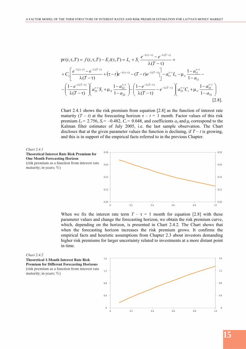
A FACTOR MODEL OF THE TERM STRUCTURE OF INTEREST RATES AND RISK PREMIUM ESTIMATION FOR LATVIAS MONEY MARKET
16
CONCLUSION The paper presents the analysis of risk premium of the interest rate term structure for the Latvian money market The risk premium has been defined as the difference between the forward interest rate and the expected future interest rate of the respective maturity The interest rate term structure is assessed consistently with the NelsonndashSiegel model On the back of the approach used by F Diebold G Rudebusch and B Aruoba it has been assumed that the coefficients of the NelsonndashSiegel model are unobservable therefore the model of this research paper has been estimated using the Kalman filter RIGIBID and RIGIBOR interest rates of the Latvian money market have been used as the observable variables The expected future interest rate has been computed as the Kalman filter forecast n periods ahead The risk premium behaviour has been obtained for interest rates of different maturities and forecasting horizons between May 2000 and July 2005 The results obtained indicate that the amount of the risk premium was significant and its volatility substantial between 2000 and 2002 In post-2002 period its behaviour gradually stabilised and was marked by a downward trend after 2004 This is in support of the assumption that with the forecasting horizon increasing the risk premium grows while with the expansion of maturity it becomes smaller These facts have been explained theoretically in the paper on the basis of the models mathematical structure The risk premium estimation becomes more complicated when the market participants expectations embedded in the financial market data are to be analysed The respective analysis carried out within this research has proposed an additional instrument for a CB to timely identify the market participants expectations regarding interest rates in the future and to learn about their confidence in the conducted monetary policy Nevertheless the employment of such instruments as money market RIGIBID and RIGIBOR restricts the forecasting horizon to one year In order to expand the forecasting horizon and to enhance the accuracy of the risk premium estimates the up-coming research foresees to include in the model the bond market data which are better determinants of the convergence process (to euro interest rates) In such circumstances the application of the Kalman filter has particular advantages for rare transactions and irregular quotations are characteristic for the government bond market of Latvia(3) In addition bond market data are non-stationary The Kalman filter has another positive trait it implicitly allows for accounting of such unobservable factors as investment and political climate whose correct quantitative estimation is impossible The including of such macroeconomic variables as inflation GDP etc (6) in the model opens up another potential area of investigation It would elucidate whether the interest rate term structure carries information that would allow for forecasting macroeconomic variables and vice versa whether macroeconomic variables allow for improving interest rate forecasts The results regarding risk premium behaviour obtained by such a method would be comparable with the findings of the factor models used in the current study it would likewise be possible to assess the accuracy of the computed risk premium
A FACTOR MODEL OF THE TERM STRUCTURE OF INTEREST RATES AND RISK PREMIUM ESTIMATION FOR LATVIAS MONEY MARKET
17
APPENDICES
Appendix 1 Detailed Description of the Kalman Filter Methodology A1 Properties of conditional mathematical expectations
x and y denote random vectors whose joint distribution has the first and the second moments The second moments are defined as
)()()()(
)()()()(
)()()()(
xEyExyExyC
yEyEyyEyD
xExExxExD
1
where denotes the transposed matrix It is assumed that the conditional expected y value with condition x (which holds at a normal joint distribution of x and y) can be written as a linear function E(yx) = α + B x 2 Vector α and matrix B will be expressed as moments of equation system 1 Using the property of conditional mathematical expectations EE(yx) = E(y) 3 from equation 2 we obtain E(y) = α + B E(x) 4 or α = E(y) ndash B E(x) 5 Multiplying equation 2 by x gives E(yx) x = α x + B x x When computing mathematical expectations for the right and left side of the equation and using equation 3 we obtain EE(yx) x = EE(y xx) = E(y x) = α E(x) + B[E (x x)] or E(y x) = α E(x) + B[E (x x)] 6 Multiplying equation 4 by E(x) we obtain E(y) E(x) = α E(x) + BE(x) E(x) 7
A FACTOR MODEL OF THE TERM STRUCTURE OF INTEREST RATES AND RISK PREMIUM ESTIMATION FOR LATVIAS MONEY MARKET
18
Subtracting equation 6 from equation 7 and using system 1 we obtain C(yx) = E(y middot x) ndash E(y) middot E(x) = B(E(x x) ndash E(x) E(x)) = BD(x) 8 thus arriving at B = C(yx)Dndash1(x) 9 Substituting B from equation 9 and α from equation 5 into equation 2 we obtain E(yx) = α + Bx = E(y) ndash BE(x) + Bx = = E(y) ndash B(x ndash E(x)) = E(y) ndash C(yx) Dndash1(x)(x ndash E(x)) or E(yx) = E(y) ndash C(yx) Dndash1(x)(x ndash E(x)) 10 The following representation is derived in a similar way D(yx) = D(y) ndash C(yx) Dndash1(x) C(xy) 11
A2 The Kalman filter The representation of (n x 1) state-space dynamics of dimensional vector yt can be defined with the following equation system yt = ct + Ztαt + εt 12 αt+1 = dt + Ttαt + vt+1 13 where αt is the (m x 1) dimensional vector of unobservable variables ct dt Zt Tt are vectors and matrices of respective dimensions εt and vt are Gaussian random vectors with zero mean Equation 12 is often referred to as the signal or observation equation while equation 13 is known as the state or transition equation Random vectors εt and vt are treated as serially uncorrelated in time with the following covariance matrix
tt
tt
t
tt QG
GH
v var 14
It is assumed that vectors εt and vt are white noises vectors ie
t
tHE t 0
)(
t
tQE t 0
)( 15
A FACTOR MODEL OF THE TERM STRUCTURE OF INTEREST RATES AND RISK PREMIUM ESTIMATION FOR LATVIAS MONEY MARKET
19
where H and Q are symmetrical matrices of (n x n) and (m x m) dimensions respectively It is also assumed that εt and vt do not correlate for all lags
0)( vE t t τ 16
The Kalman filter is applied for an optimal estimation of vector αt of unobservable variables and for estimation updating when new values of observable variables become available Optimal forecasts for endogenous variable yt are acquired at the same time We assume the need to calculate tt ndash the optimal estimate (with minimum mean
squared error) t using information available up to time t and tt which is the error
covariance matrix for the forecast in state equations It is also assumed that vectors c and d as well as matrices Z and T are known The recurrent algorithm of the Kalman filter includes the following steps 1 Selection of the initial state α10 denotes the predicted value of α1 which is based on the initial value of y0 If all eigenvalues of matrix T are smaller than 1 by their absolute values it is assumed that α10 = E(α1) ie unconditional mean value of the process We assume that Ω10 satisfies the equation Ω10 = T Ω10 T + Q 17 which is consistent with unconditional covariance matrix of the process If some eigenvalues of matrix T exceed or are equal to unit the unconditional mean of the process and covariance cannot be selected as initial values (as not existing) and hence the selection shall be made on the back of other considerations When the initial values α10 and Ω10 are known the next action is to calculate α21 and Ω21 for the next time moment As all computations for periods t = 2 3 T are analogous the transition computation algorithm for any period t from values αttndash1 Ωttndash1 to values αt+1t Ω
t+1t is used
2 Yt predicting and construction of its covariance matrix
11
tttt Zcy 18
HZZEyyyyE tttttttttttt ))((())(( 1111
= 11
tttt HZZ 19
3 Assuming that yt value becomes available at time t This information allows for the adjustment of forecast 1 ttt
Ytndash1 denotes vector (y0 y1 ytndash1) Thus from equation 12 we obtain
A FACTOR MODEL OF THE TERM STRUCTURE OF INTEREST RATES AND RISK PREMIUM ESTIMATION FOR LATVIAS MONEY MARKET
20
)cov()cov( 11 tttttt YZYy
)))((( 1111 ZYZE ttttttttt
HZZYZcDYyD ttttttt 111 )()(
11)( tttt YE
Using equation 10 (substituting y with αt x with yt and replacing the unconditional mathematical expectation with equation E(Ytndash1)) we obtain the adjusted value of tt
)(]))([(]))([( 11
11111
ttttttttttttttttttt yyyyyyEyyE
20 while
)]))(([(]))([( 1111 ttttttttttttt ZEyyE
= ]))([( 111 ZZE tttttttt
21
The condition that t is uncorrelated to other factors is used
Substituting equation 19 into equation 20 we obtain
)()( 11
111
ttttttttttt ZcyHZZZ 22
Covariance matrix for errors related to the given adjusted forecast is obtained from equation 11
]))([( tttttttt E
]))([(]))([( 1111 tttttttttttt yyEE
]))([(]))([( 111
11 tttttttttttt yyEyyyyE
= 11
111 )(
tttttttt ZHZZZ 23
The difference between the adjusted value tt and value 1 tt which was predicted
before information about yt became available is presented as
)()( 11
11
ttttttt ZcyHZZZ Hence the larger the value of the
expression 11 tttttt yyZcy ie the difference between the realised and
predicted value of yt the larger the adjustment ( tt ndash 1 tt ) however the given value is
inversely proportional to the forecasting accuracy which is consistent with
1 1
tt tt HZZ and directly proportional to covariance between αt and
yt ndash 1Ztt Consequently the less accurate the forecast 1tty the smaller the value of
the adjustment term in equation 23 and the larger the conditional covariance between αt and yt the larger the adjustment term
A FACTOR MODEL OF THE TERM STRUCTURE OF INTEREST RATES AND RISK PREMIUM ESTIMATION FOR LATVIAS MONEY MARKET
21
4 Derivation of the state variable forecast for the next period from equation 13
ttttttttttttt TdYvEYETdYvTdEYE )()()()( 1111
24 Substituting equation 22 into equation 24 we obtain
)()( 11
1111
ttttttttttt ZcyHZZZTTd 25
Matrix
111 )( HZZZTk ttttt 26
is known as the gain matrix and equation 25 can be rewritten
)( 111 ttttttt ZcykTd 27
The measurement error covariance matrix for this forecast can be computed using equations 13 and 24
]))([( 11111 tttttttt E
]))([( 11 tttttttt TdvTdTdvTdE
ttttttttttt QTTvvETET )(]))([( 11 28
Substitution of equation 23 into equation 28 results in
ttttttttttt QTZHZZZT
])([ 11
1111 29
A3 Applying the Kalman filter to forecasts n periods ahead
Via recursive substitution equation 13 produces
ntnttn
tn
tn
nt vvTvTvTT
11
22
11 where n = 1 2 3hellip 30
Projecting nt to t and tY we obtain
tn
ttnt TYE )(
The application of conditional mathematical expectations property leads to
ttn
ttn
ttn
tttnttnttnt TYETYTEYYEEYE )()(])([)( 31
From forecast equations of expressions 30 and 31 n-periods ahead it follows that
A FACTOR MODEL OF THE TERM STRUCTURE OF INTEREST RATES AND RISK PREMIUM ESTIMATION FOR LATVIAS MONEY MARKET
22
ntnttn
tn
tttn
tntnt vvTvTvTT
11
22
11 )( 32
The measurement error covariance matrix is
QTQTTQTTQTTT nnnnntt
ntnt
)()()( 2211 33
The following expression for the observed vector is obtained from equation 12
ntntnt Zcy
Consequently y forecast for n periods ahead can be computed using the relationship
tnttnttnt ZcYyEy )( 34
The forecast error in turn is characterised by the following relationship
nttntnttntntnttntnt ZZcZcyy )()()(
The covariance matrix of this error is as follows
HZZyyyyE tnttntnttntnt ]))([(
A4 The Kalman filter in model parameter estimation
If the initial state of 1 and random vectors )( tt v are of the Gaussian type ty
distribution meeting condition 1tY also is Gaussian with the mean
11 tttt Zcy
and the measurement error matrix
1 1
tt tt HZZ
The distribution density is represented by
2
1
12
1 )2()( HZZYyf tt
n
tt
)()()(2
1exp 1
111
tttttttt ZcyHZZZcy 35
where t = 1 2 T
)( 1 Tyyf represents the total vector density )( 1 Tyy Taking into account the total density property it can be represented as follows
A FACTOR MODEL OF THE TERM STRUCTURE OF INTEREST RATES AND RISK PREMIUM ESTIMATION FOR LATVIAS MONEY MARKET
23
)()()( 11111 yyfyyyfyyf TTTT
)()()( 11
2
012111 yyyfyyyfyyyf jT
T
jjTTTTT
36
Taking log of equation 33 and using equation 32 the following likelihood function is derived
])()[(2
1log
2
12log
2)(
1
1 11
11
11
tt ttt
T
tttT
T
tttT yyyy
TnyyL
37 where φ is the parameter vector
11 )0(~
ttttt Nyy 011 )(~ yNy
where y is the unconditional mean of the process
A5 Model parameter computation algorithm 1 Initial parameter vector 0 is selected
2 Steps 1ndash4 of the Kalman filter recurrent algorithm are taken (see A2)
3 For each step computations are conducted for 1 ttt yy and 1ttthat are
included in the formation of the likelihood function of equation 35 4 The new value of parameter vector i which increases L in equation 37 is derived
by one of the numerical methods 5 Time steps 2ndash4 of the Kalman filter recurrent algorithm (see A2) are repeated until
1ii and )(L
with sufficiently small value
A FACTOR MODEL OF THE TERM STRUCTURE OF INTEREST RATES AND RISK PREMIUM ESTIMATION FOR LATVIAS MONEY MARKET
24
Appendix 2 1-Month Interest Rate Risk Premium Dynamics for Different Forecasting Horizons (prij is premium for forecasting horizon i (in months) with repayment period j (in months) )
04
08
12
16
20
24
2000 2001 2002 2003 2004 2005
pr910
04
08
12
16
20
24
2000 2001 2002 2003 2004 2005
pr1011
04
08
12
16
20
24
2000 2001 2002 2003 2004 2005
pr1112
06
08
10
12
14
16
18
20
22
2000 2001 2002 2003 2004 2005
pr1213
ndash01
0
01 02 03 04 05 06 07
2000 2001 2002 2003 2004 2005
p r 1 2 ndash02
0
02
04
06
08
10
12
2000 2001 2002 2003 2004 2005
pr23
ndash04
0
04
08
12
16
2000 2001 2002 2003 2004 2005 pr34
ndash04 00
04
08
12
16
20
2000 2001 2002 2003 2004 2005
pr45
0 04
08
12
16
20
2000 2001 2002 2003 2004 2005 p r 56
0
04
08
12
16
20
2000 2001 2002 2003 2004 2005
pr67
0
04
08
12
16
20
24
2000 2001 2002 2003 2004 2005 pr78
0
04
08
12
16
20
24
2000 2001 2002 2003 2004 2005
pr89
A FACTOR MODEL OF THE TERM STRUCTURE OF INTEREST RATES AND RISK PREMIUM ESTIMATION FOR LATVIAS MONEY MARKET
25
Appendix 3 3-Month Interest Rate Risk Premium Dynamics for Different Forecasting Horizons (prij is premium for forecasting horizon i (in months) with repayment period j (in months) )
00
04
08
12
16
20
2000 2001 2002 2003 2004 2005
pr58
04
08
12
16
20
2000 2001 2002 2003 2004 2005
pr912
04
06
08
10
12
14
16
18
20
2000 2001 2002 2003 2004 2005
pr1013
06
08
10
12
14
16
18
20
2000 2001 2002 2003 2004 2005
pr1114
06
08
10
12
14
16
18
20
2000 2001 2002 2003 2004 2005
pr1215
ndash01
0
01
02
03
04
05
06
2000 2001 2002 2003 2004 2005
p r 1 4 ndash02
0 02 04 06 08 10
2000 2001 2002 2003 2004 2005
pr25
0
02
04
06
08
10
12
14
2000 2001 2002 2003 2004 2005 pr36
0 02 04 06 08 10 12 14 16
2000 2001 2002 2003 2004 2005
pr47
0 04 08 12 16 20
2000 2001 2002 2003 2004 2005
pr811
0
04
08
12
16
20
2000 2001 2002 2003 2004 2005 pr710
0 04 08 12 16 20
2000 2001 2002 2003 2004 2005
pr69
ndash02
A FACTOR MODEL OF THE TERM STRUCTURE OF INTEREST RATES AND RISK PREMIUM ESTIMATION FOR LATVIAS MONEY MARKET
26
Appendix 4 6-Month Interest Rate Risk Premium Dynamics for Different Forecasting Horizons (prij is premium for forecasting horizon i (in months) with repayment period j (in months) )
02
04
06
08
10
12
14
16
2000 2001 2002 2003 2004 2005
pr612
02
04
06
08
10
12
14
16
2000 2001 2002 2003 2004 2005
pr713
02
04
06
08
10
12
14
16
18
2000 2001 2002 2003 2004 2005
pr814
04
06
08
10
12
14
16
18
2000 2001 2002 2003 2004 2005
pr915
04
06
08
10
12
14
16
18
2000 2001 2002 2003 2004 2005
pr1016
06
08
10
12
14
16
18
2000 2001 2002 2003 2004 2005
pr1117
06
08
10
12
14
16
18
2000 2001 2002 2003 2004 2005
pr1218
ndash01
0 01 02 03 04 05
2000 2001 2002 2003 2004 2005
pr 1 7ndash01
0
01
02
03
04
05
06
07
08
2000 2001 2002 2003 2004 2005
pr28
0
02
04
06
08
10
12
2000 2001 2002 2003 2004 2005
pr39
0 02 04 06 08 10 12 14
2000 2001 2002 2003 2004 2005
pr410
0 02
04
06
08
10
12
14
2000 2001 2002 2003 2004 2005
p r 5 1 1
A FACTOR MODEL OF THE TERM STRUCTURE OF INTEREST RATES AND RISK PREMIUM ESTIMATION FOR LATVIAS MONEY MARKET
27
Appendix 5 12-Month Interest Rate Risk Premium Dynamics for Different Forcasting Horizons (prij is premium for forecasting horizon i (in months) with repayment period j (in months) )
01
02
03
04
05
06
07
08
09
10
2000 2001 2002 2003 2004 2005
pr416
02
04
06
08
10
12
2000 2001 2002 2003 2004 2005
pr618
03
04
05
06
07
08
09
10
11
12
2000 2001 2002 2003 2004 2005
pr719
04
05
06
07
08
09
10
11
12
13
2000 2001 2002 2003 2004 2005
pr820
05
06
07
08
09
10
11
12
13
2000 2001 2002 2003 2004 2005
pr921
05
06
07
08
09
10
11
12
13
14
2000 2001 2002 2003 2004 2005
pr1022
06
07
08
09
10
11
12
13
14
2000 2001 2002 2003 2004 2005
pr1123
07
08
09
10
11
12
13
14
2000 2001 2002 2003 2004 2005
pr1224
ndash005
0 005
010
015
020
025
030
035
2000 2001 2002 2003 2004 2005
p r 11 3 0
01 02 03 04 05 06
2000 2001 2002 2003 2004 2005
pr214
0
01
02
03
04
05
06
07
08
2000 2001 2002 2003 2004 2005
pr315
0
02
04
06
08
10
12
2000 2001 2002 2003 2004 2005 pr 5 17
A FACTOR MODEL OF THE TERM STRUCTURE OF INTEREST RATES AND RISK PREMIUM ESTIMATION FOR LATVIAS MONEY MARKET
28
Appendix 6 Mean Interest Rate Risk Premium and Standard Deviation (prij is premium for forecasting horizon i (in months) with repayment period j (in months) ) On 1-month interest rate
pr12 pr23 pr34 pr45 pr56 pr67 pr78 pr89 pr910 pr1011 pr1112 pr1213 Mean premium 0193629 0364347 0515686 0650680 0771919 0881606 0981610 1073508 1158631 1238101 1312857 1383688Standard deviation 0124962 0211080 0267350 0300950 0317572 0321701 0316850 0305745 0290489 0272687 0253551 0233989
On 3-month interest rate
pr14 pr25 pr36 pr47 pr58 pr69 pr710 pr811 pr912 pr1013 pr1114 pr1215 Mean premium 0175572 0331301 0470243 0595022 0707878 0810715 0905146 0992536 1074034 1150609 1223071 1292104Standard deviation 0106270 0179455 0227233 0255724 0269783 0273233 0269068 0259613 0246660 0231579 0215408 0198923
On 6-month interest rate
pr17 pr28 pr39 pr410 pr511 pr612 pr713 pr814 pr915 pr1016 pr1117 pr1218 Mean premium 0154646 0293008 0417591 0530540 0633689 0728594 0816575 0898746 0976048 1049272 1119081 1186033Standard deviation 0084945 0143384 0181485 0204165 0215318 0218016 0214659 0207116 0196827 0184895 0172159 0159248
On 12-month interest rate
pr113 pr214 pr315 pr416 pr517 pr618 pr719 pr820 pr921 pr1022 pr1123 pr1224 Mean premium 0127464 0243277 0349219 0446817 0537372 0621988 0701603 0777008 0848869 0917749 0984119 1048375Standard deviation 0057915 0097684 0123556 0138914 0146443 0148255 0146006 0140985 0134193 0126398 0118191 0110020
A FACTOR MODEL OF THE TERM STRUCTURE OF INTEREST RATES AND RISK PREMIUM ESTIMATION FOR LATVIAS MONEY MARKET
29
BIBLIOGRAPHY 1 ANG Andrew PIAZZESI Monika A No-Arbitrage Vector Autoregression of Term Structure Dynamics with Macroeconomic and Latent Variables Journal of Monetary Economics vol 50 issue 4 May 2003 pp 745ndash787 2 CASSOLA Nuno LUIacuteS Barros Jorge A Two-factor Model of the German Term Structure of Interest Rates ECB Working Paper No 46 March 2001 3 CORTAZAR Gonzalo SCHWARTZ Eduardo S NARANJO Lorenzo Term Structure Estimation in Low-Frequency Transaction Markets A Kalman Filter Approach with Incomplete Panel-Data The Anderson School at UCLA Finance Working Paper No 6-03 2003 4 DIEBOLD Francis X LI Canlin Forecasting the Term Structure of Government Bond Yields NBER Working Paper No 10048 2003 5 DIEBOLD Francis X PIAZZESI Monika RUDEBUSCH Glenn D Modeling Bond Yields in Finance and Macroeconomics NBER Working Paper No 11089 2005 6 DIEBOLD Francis X RUDEBUSCH Glenn D ARUOBA Boragan S The Macroeconomy and the Yield Curve A Dynamic Latent Factor Approach NBER Working Paper No 10616 July 2004 7 DUFFEE Gregory R Term Premia and Interest Rate Forecasts in Affine Models Journal of Finance vol 57 No 1 February 2002 pp 405ndash443 8 DURREacute Alain EVJEN Snorre PILEGAARD Rasmus Estimating Risk Premia in Money Market Rates ECB Working Paper No 221 2003 9 EVANS Charles L MARSHALL David Monetary Policy and the Term Structure of Nominal Interest Rates Evidence and Theory Carnegie-Rochester Conference Series on Public Policy vol 49 1998 pp 53ndash111 10 EVANS Charles L MARSHALL David Economic Determinants of the Nominal Treasury Yield Curve Federal Reserve Bank of Chicago Working Papers No 16 2001 11 FRANKEL Jeffrey Alexander LOWN Cara S An Indicator of Future Inflation Extracted from the Steepness of the Interest Rate Yield Curve along its Entire Length Quarterly Journal of Economics vol 109 1994 pp 517ndash530 12 GRAVELLE Toni MULLER Philippe STREacuteLISKI David Towards a New Measure of Interest Rate Expectations in Canada Estimating a Time-Varying Term Premium Bank of Canada Proceedings of a Conference Information in Financial Asset Prices May 1998 13 HAMILTON James D Time Series Analysis Princeton University Press 1994 14 KENDALL Maurice G STUART Alan The Advanced Theory of Statistics London Griffin 1968 15 KNEZ Peter J LITTERMAN Robert SCHEINKMAN Joseacute Explorations into Factors Explaining Money Market Returns Journal of Finance vol 49 No 5 December 1994 pp 1861ndash1882 16 LITTERMAN Robert SCHEINKMAN Joseacute Common Factors Affecting Bond Returns Journal of Fixed Income vol 1 June 1991 pp 54ndash61
A FACTOR MODEL OF THE TERM STRUCTURE OF INTEREST RATES AND RISK PREMIUM ESTIMATION FOR LATVIAS MONEY MARKET
30
17 NELSON Charles R SIEGEL Andrew F Parsimonious Modeling of Yield Curves Journal of Business vol 60 1987 pp 473ndash489 18 SHILLER Robert J The Term Structure of Interest Rates B Friedman and F Hahn (eds) Handbook of Monetary Economics vol 1 Amsterdam North-Holland 1990 pp 627ndash722 19 The Stability-Oriented Monetary Policy Strategy of the Eurosystem ECB Monthly Bulletin No 1 January 1999 pp 39ndash505
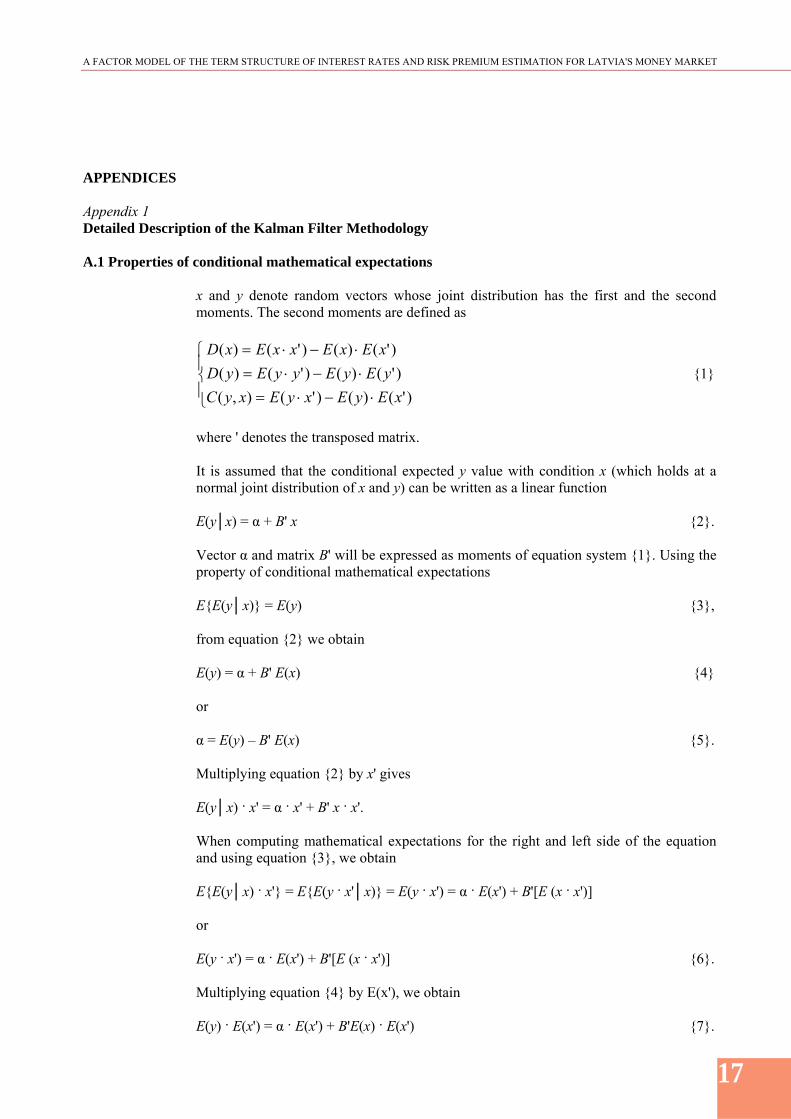
A FACTOR MODEL OF THE TERM STRUCTURE OF INTEREST RATES AND RISK PREMIUM ESTIMATION FOR LATVIAS MONEY MARKET
18
Subtracting equation 6 from equation 7 and using system 1 we obtain C(yx) = E(y middot x) ndash E(y) middot E(x) = B(E(x x) ndash E(x) E(x)) = BD(x) 8 thus arriving at B = C(yx)Dndash1(x) 9 Substituting B from equation 9 and α from equation 5 into equation 2 we obtain E(yx) = α + Bx = E(y) ndash BE(x) + Bx = = E(y) ndash B(x ndash E(x)) = E(y) ndash C(yx) Dndash1(x)(x ndash E(x)) or E(yx) = E(y) ndash C(yx) Dndash1(x)(x ndash E(x)) 10 The following representation is derived in a similar way D(yx) = D(y) ndash C(yx) Dndash1(x) C(xy) 11
A2 The Kalman filter The representation of (n x 1) state-space dynamics of dimensional vector yt can be defined with the following equation system yt = ct + Ztαt + εt 12 αt+1 = dt + Ttαt + vt+1 13 where αt is the (m x 1) dimensional vector of unobservable variables ct dt Zt Tt are vectors and matrices of respective dimensions εt and vt are Gaussian random vectors with zero mean Equation 12 is often referred to as the signal or observation equation while equation 13 is known as the state or transition equation Random vectors εt and vt are treated as serially uncorrelated in time with the following covariance matrix
tt
tt
t
tt QG
GH
v var 14
It is assumed that vectors εt and vt are white noises vectors ie
t
tHE t 0
)(
t
tQE t 0
)( 15
A FACTOR MODEL OF THE TERM STRUCTURE OF INTEREST RATES AND RISK PREMIUM ESTIMATION FOR LATVIAS MONEY MARKET
19
where H and Q are symmetrical matrices of (n x n) and (m x m) dimensions respectively It is also assumed that εt and vt do not correlate for all lags
0)( vE t t τ 16
The Kalman filter is applied for an optimal estimation of vector αt of unobservable variables and for estimation updating when new values of observable variables become available Optimal forecasts for endogenous variable yt are acquired at the same time We assume the need to calculate tt ndash the optimal estimate (with minimum mean
squared error) t using information available up to time t and tt which is the error
covariance matrix for the forecast in state equations It is also assumed that vectors c and d as well as matrices Z and T are known The recurrent algorithm of the Kalman filter includes the following steps 1 Selection of the initial state α10 denotes the predicted value of α1 which is based on the initial value of y0 If all eigenvalues of matrix T are smaller than 1 by their absolute values it is assumed that α10 = E(α1) ie unconditional mean value of the process We assume that Ω10 satisfies the equation Ω10 = T Ω10 T + Q 17 which is consistent with unconditional covariance matrix of the process If some eigenvalues of matrix T exceed or are equal to unit the unconditional mean of the process and covariance cannot be selected as initial values (as not existing) and hence the selection shall be made on the back of other considerations When the initial values α10 and Ω10 are known the next action is to calculate α21 and Ω21 for the next time moment As all computations for periods t = 2 3 T are analogous the transition computation algorithm for any period t from values αttndash1 Ωttndash1 to values αt+1t Ω
t+1t is used
2 Yt predicting and construction of its covariance matrix
11
tttt Zcy 18
HZZEyyyyE tttttttttttt ))((())(( 1111
= 11
tttt HZZ 19
3 Assuming that yt value becomes available at time t This information allows for the adjustment of forecast 1 ttt
Ytndash1 denotes vector (y0 y1 ytndash1) Thus from equation 12 we obtain
A FACTOR MODEL OF THE TERM STRUCTURE OF INTEREST RATES AND RISK PREMIUM ESTIMATION FOR LATVIAS MONEY MARKET
20
)cov()cov( 11 tttttt YZYy
)))((( 1111 ZYZE ttttttttt
HZZYZcDYyD ttttttt 111 )()(
11)( tttt YE
Using equation 10 (substituting y with αt x with yt and replacing the unconditional mathematical expectation with equation E(Ytndash1)) we obtain the adjusted value of tt
)(]))([(]))([( 11
11111
ttttttttttttttttttt yyyyyyEyyE
20 while
)]))(([(]))([( 1111 ttttttttttttt ZEyyE
= ]))([( 111 ZZE tttttttt
21
The condition that t is uncorrelated to other factors is used
Substituting equation 19 into equation 20 we obtain
)()( 11
111
ttttttttttt ZcyHZZZ 22
Covariance matrix for errors related to the given adjusted forecast is obtained from equation 11
]))([( tttttttt E
]))([(]))([( 1111 tttttttttttt yyEE
]))([(]))([( 111
11 tttttttttttt yyEyyyyE
= 11
111 )(
tttttttt ZHZZZ 23
The difference between the adjusted value tt and value 1 tt which was predicted
before information about yt became available is presented as
)()( 11
11
ttttttt ZcyHZZZ Hence the larger the value of the
expression 11 tttttt yyZcy ie the difference between the realised and
predicted value of yt the larger the adjustment ( tt ndash 1 tt ) however the given value is
inversely proportional to the forecasting accuracy which is consistent with
1 1
tt tt HZZ and directly proportional to covariance between αt and
yt ndash 1Ztt Consequently the less accurate the forecast 1tty the smaller the value of
the adjustment term in equation 23 and the larger the conditional covariance between αt and yt the larger the adjustment term
A FACTOR MODEL OF THE TERM STRUCTURE OF INTEREST RATES AND RISK PREMIUM ESTIMATION FOR LATVIAS MONEY MARKET
21
4 Derivation of the state variable forecast for the next period from equation 13
ttttttttttttt TdYvEYETdYvTdEYE )()()()( 1111
24 Substituting equation 22 into equation 24 we obtain
)()( 11
1111
ttttttttttt ZcyHZZZTTd 25
Matrix
111 )( HZZZTk ttttt 26
is known as the gain matrix and equation 25 can be rewritten
)( 111 ttttttt ZcykTd 27
The measurement error covariance matrix for this forecast can be computed using equations 13 and 24
]))([( 11111 tttttttt E
]))([( 11 tttttttt TdvTdTdvTdE
ttttttttttt QTTvvETET )(]))([( 11 28
Substitution of equation 23 into equation 28 results in
ttttttttttt QTZHZZZT
])([ 11
1111 29
A3 Applying the Kalman filter to forecasts n periods ahead
Via recursive substitution equation 13 produces
ntnttn
tn
tn
nt vvTvTvTT
11
22
11 where n = 1 2 3hellip 30
Projecting nt to t and tY we obtain
tn
ttnt TYE )(
The application of conditional mathematical expectations property leads to
ttn
ttn
ttn
tttnttnttnt TYETYTEYYEEYE )()(])([)( 31
From forecast equations of expressions 30 and 31 n-periods ahead it follows that
A FACTOR MODEL OF THE TERM STRUCTURE OF INTEREST RATES AND RISK PREMIUM ESTIMATION FOR LATVIAS MONEY MARKET
22
ntnttn
tn
tttn
tntnt vvTvTvTT
11
22
11 )( 32
The measurement error covariance matrix is
QTQTTQTTQTTT nnnnntt
ntnt
)()()( 2211 33
The following expression for the observed vector is obtained from equation 12
ntntnt Zcy
Consequently y forecast for n periods ahead can be computed using the relationship
tnttnttnt ZcYyEy )( 34
The forecast error in turn is characterised by the following relationship
nttntnttntntnttntnt ZZcZcyy )()()(
The covariance matrix of this error is as follows
HZZyyyyE tnttntnttntnt ]))([(
A4 The Kalman filter in model parameter estimation
If the initial state of 1 and random vectors )( tt v are of the Gaussian type ty
distribution meeting condition 1tY also is Gaussian with the mean
11 tttt Zcy
and the measurement error matrix
1 1
tt tt HZZ
The distribution density is represented by
2
1
12
1 )2()( HZZYyf tt
n
tt
)()()(2
1exp 1
111
tttttttt ZcyHZZZcy 35
where t = 1 2 T
)( 1 Tyyf represents the total vector density )( 1 Tyy Taking into account the total density property it can be represented as follows
A FACTOR MODEL OF THE TERM STRUCTURE OF INTEREST RATES AND RISK PREMIUM ESTIMATION FOR LATVIAS MONEY MARKET
23
)()()( 11111 yyfyyyfyyf TTTT
)()()( 11
2
012111 yyyfyyyfyyyf jT
T
jjTTTTT
36
Taking log of equation 33 and using equation 32 the following likelihood function is derived
])()[(2
1log
2
12log
2)(
1
1 11
11
11
tt ttt
T
tttT
T
tttT yyyy
TnyyL
37 where φ is the parameter vector
11 )0(~
ttttt Nyy 011 )(~ yNy
where y is the unconditional mean of the process
A5 Model parameter computation algorithm 1 Initial parameter vector 0 is selected
2 Steps 1ndash4 of the Kalman filter recurrent algorithm are taken (see A2)
3 For each step computations are conducted for 1 ttt yy and 1ttthat are
included in the formation of the likelihood function of equation 35 4 The new value of parameter vector i which increases L in equation 37 is derived
by one of the numerical methods 5 Time steps 2ndash4 of the Kalman filter recurrent algorithm (see A2) are repeated until
1ii and )(L
with sufficiently small value
A FACTOR MODEL OF THE TERM STRUCTURE OF INTEREST RATES AND RISK PREMIUM ESTIMATION FOR LATVIAS MONEY MARKET
24
Appendix 2 1-Month Interest Rate Risk Premium Dynamics for Different Forecasting Horizons (prij is premium for forecasting horizon i (in months) with repayment period j (in months) )
04
08
12
16
20
24
2000 2001 2002 2003 2004 2005
pr910
04
08
12
16
20
24
2000 2001 2002 2003 2004 2005
pr1011
04
08
12
16
20
24
2000 2001 2002 2003 2004 2005
pr1112
06
08
10
12
14
16
18
20
22
2000 2001 2002 2003 2004 2005
pr1213
ndash01
0
01 02 03 04 05 06 07
2000 2001 2002 2003 2004 2005
p r 1 2 ndash02
0
02
04
06
08
10
12
2000 2001 2002 2003 2004 2005
pr23
ndash04
0
04
08
12
16
2000 2001 2002 2003 2004 2005 pr34
ndash04 00
04
08
12
16
20
2000 2001 2002 2003 2004 2005
pr45
0 04
08
12
16
20
2000 2001 2002 2003 2004 2005 p r 56
0
04
08
12
16
20
2000 2001 2002 2003 2004 2005
pr67
0
04
08
12
16
20
24
2000 2001 2002 2003 2004 2005 pr78
0
04
08
12
16
20
24
2000 2001 2002 2003 2004 2005
pr89
A FACTOR MODEL OF THE TERM STRUCTURE OF INTEREST RATES AND RISK PREMIUM ESTIMATION FOR LATVIAS MONEY MARKET
25
Appendix 3 3-Month Interest Rate Risk Premium Dynamics for Different Forecasting Horizons (prij is premium for forecasting horizon i (in months) with repayment period j (in months) )
00
04
08
12
16
20
2000 2001 2002 2003 2004 2005
pr58
04
08
12
16
20
2000 2001 2002 2003 2004 2005
pr912
04
06
08
10
12
14
16
18
20
2000 2001 2002 2003 2004 2005
pr1013
06
08
10
12
14
16
18
20
2000 2001 2002 2003 2004 2005
pr1114
06
08
10
12
14
16
18
20
2000 2001 2002 2003 2004 2005
pr1215
ndash01
0
01
02
03
04
05
06
2000 2001 2002 2003 2004 2005
p r 1 4 ndash02
0 02 04 06 08 10
2000 2001 2002 2003 2004 2005
pr25
0
02
04
06
08
10
12
14
2000 2001 2002 2003 2004 2005 pr36
0 02 04 06 08 10 12 14 16
2000 2001 2002 2003 2004 2005
pr47
0 04 08 12 16 20
2000 2001 2002 2003 2004 2005
pr811
0
04
08
12
16
20
2000 2001 2002 2003 2004 2005 pr710
0 04 08 12 16 20
2000 2001 2002 2003 2004 2005
pr69
ndash02
A FACTOR MODEL OF THE TERM STRUCTURE OF INTEREST RATES AND RISK PREMIUM ESTIMATION FOR LATVIAS MONEY MARKET
26
Appendix 4 6-Month Interest Rate Risk Premium Dynamics for Different Forecasting Horizons (prij is premium for forecasting horizon i (in months) with repayment period j (in months) )
02
04
06
08
10
12
14
16
2000 2001 2002 2003 2004 2005
pr612
02
04
06
08
10
12
14
16
2000 2001 2002 2003 2004 2005
pr713
02
04
06
08
10
12
14
16
18
2000 2001 2002 2003 2004 2005
pr814
04
06
08
10
12
14
16
18
2000 2001 2002 2003 2004 2005
pr915
04
06
08
10
12
14
16
18
2000 2001 2002 2003 2004 2005
pr1016
06
08
10
12
14
16
18
2000 2001 2002 2003 2004 2005
pr1117
06
08
10
12
14
16
18
2000 2001 2002 2003 2004 2005
pr1218
ndash01
0 01 02 03 04 05
2000 2001 2002 2003 2004 2005
pr 1 7ndash01
0
01
02
03
04
05
06
07
08
2000 2001 2002 2003 2004 2005
pr28
0
02
04
06
08
10
12
2000 2001 2002 2003 2004 2005
pr39
0 02 04 06 08 10 12 14
2000 2001 2002 2003 2004 2005
pr410
0 02
04
06
08
10
12
14
2000 2001 2002 2003 2004 2005
p r 5 1 1
A FACTOR MODEL OF THE TERM STRUCTURE OF INTEREST RATES AND RISK PREMIUM ESTIMATION FOR LATVIAS MONEY MARKET
27
Appendix 5 12-Month Interest Rate Risk Premium Dynamics for Different Forcasting Horizons (prij is premium for forecasting horizon i (in months) with repayment period j (in months) )
01
02
03
04
05
06
07
08
09
10
2000 2001 2002 2003 2004 2005
pr416
02
04
06
08
10
12
2000 2001 2002 2003 2004 2005
pr618
03
04
05
06
07
08
09
10
11
12
2000 2001 2002 2003 2004 2005
pr719
04
05
06
07
08
09
10
11
12
13
2000 2001 2002 2003 2004 2005
pr820
05
06
07
08
09
10
11
12
13
2000 2001 2002 2003 2004 2005
pr921
05
06
07
08
09
10
11
12
13
14
2000 2001 2002 2003 2004 2005
pr1022
06
07
08
09
10
11
12
13
14
2000 2001 2002 2003 2004 2005
pr1123
07
08
09
10
11
12
13
14
2000 2001 2002 2003 2004 2005
pr1224
ndash005
0 005
010
015
020
025
030
035
2000 2001 2002 2003 2004 2005
p r 11 3 0
01 02 03 04 05 06
2000 2001 2002 2003 2004 2005
pr214
0
01
02
03
04
05
06
07
08
2000 2001 2002 2003 2004 2005
pr315
0
02
04
06
08
10
12
2000 2001 2002 2003 2004 2005 pr 5 17
A FACTOR MODEL OF THE TERM STRUCTURE OF INTEREST RATES AND RISK PREMIUM ESTIMATION FOR LATVIAS MONEY MARKET
28
Appendix 6 Mean Interest Rate Risk Premium and Standard Deviation (prij is premium for forecasting horizon i (in months) with repayment period j (in months) ) On 1-month interest rate
pr12 pr23 pr34 pr45 pr56 pr67 pr78 pr89 pr910 pr1011 pr1112 pr1213 Mean premium 0193629 0364347 0515686 0650680 0771919 0881606 0981610 1073508 1158631 1238101 1312857 1383688Standard deviation 0124962 0211080 0267350 0300950 0317572 0321701 0316850 0305745 0290489 0272687 0253551 0233989
On 3-month interest rate
pr14 pr25 pr36 pr47 pr58 pr69 pr710 pr811 pr912 pr1013 pr1114 pr1215 Mean premium 0175572 0331301 0470243 0595022 0707878 0810715 0905146 0992536 1074034 1150609 1223071 1292104Standard deviation 0106270 0179455 0227233 0255724 0269783 0273233 0269068 0259613 0246660 0231579 0215408 0198923
On 6-month interest rate
pr17 pr28 pr39 pr410 pr511 pr612 pr713 pr814 pr915 pr1016 pr1117 pr1218 Mean premium 0154646 0293008 0417591 0530540 0633689 0728594 0816575 0898746 0976048 1049272 1119081 1186033Standard deviation 0084945 0143384 0181485 0204165 0215318 0218016 0214659 0207116 0196827 0184895 0172159 0159248
On 12-month interest rate
pr113 pr214 pr315 pr416 pr517 pr618 pr719 pr820 pr921 pr1022 pr1123 pr1224 Mean premium 0127464 0243277 0349219 0446817 0537372 0621988 0701603 0777008 0848869 0917749 0984119 1048375Standard deviation 0057915 0097684 0123556 0138914 0146443 0148255 0146006 0140985 0134193 0126398 0118191 0110020
A FACTOR MODEL OF THE TERM STRUCTURE OF INTEREST RATES AND RISK PREMIUM ESTIMATION FOR LATVIAS MONEY MARKET
29
BIBLIOGRAPHY 1 ANG Andrew PIAZZESI Monika A No-Arbitrage Vector Autoregression of Term Structure Dynamics with Macroeconomic and Latent Variables Journal of Monetary Economics vol 50 issue 4 May 2003 pp 745ndash787 2 CASSOLA Nuno LUIacuteS Barros Jorge A Two-factor Model of the German Term Structure of Interest Rates ECB Working Paper No 46 March 2001 3 CORTAZAR Gonzalo SCHWARTZ Eduardo S NARANJO Lorenzo Term Structure Estimation in Low-Frequency Transaction Markets A Kalman Filter Approach with Incomplete Panel-Data The Anderson School at UCLA Finance Working Paper No 6-03 2003 4 DIEBOLD Francis X LI Canlin Forecasting the Term Structure of Government Bond Yields NBER Working Paper No 10048 2003 5 DIEBOLD Francis X PIAZZESI Monika RUDEBUSCH Glenn D Modeling Bond Yields in Finance and Macroeconomics NBER Working Paper No 11089 2005 6 DIEBOLD Francis X RUDEBUSCH Glenn D ARUOBA Boragan S The Macroeconomy and the Yield Curve A Dynamic Latent Factor Approach NBER Working Paper No 10616 July 2004 7 DUFFEE Gregory R Term Premia and Interest Rate Forecasts in Affine Models Journal of Finance vol 57 No 1 February 2002 pp 405ndash443 8 DURREacute Alain EVJEN Snorre PILEGAARD Rasmus Estimating Risk Premia in Money Market Rates ECB Working Paper No 221 2003 9 EVANS Charles L MARSHALL David Monetary Policy and the Term Structure of Nominal Interest Rates Evidence and Theory Carnegie-Rochester Conference Series on Public Policy vol 49 1998 pp 53ndash111 10 EVANS Charles L MARSHALL David Economic Determinants of the Nominal Treasury Yield Curve Federal Reserve Bank of Chicago Working Papers No 16 2001 11 FRANKEL Jeffrey Alexander LOWN Cara S An Indicator of Future Inflation Extracted from the Steepness of the Interest Rate Yield Curve along its Entire Length Quarterly Journal of Economics vol 109 1994 pp 517ndash530 12 GRAVELLE Toni MULLER Philippe STREacuteLISKI David Towards a New Measure of Interest Rate Expectations in Canada Estimating a Time-Varying Term Premium Bank of Canada Proceedings of a Conference Information in Financial Asset Prices May 1998 13 HAMILTON James D Time Series Analysis Princeton University Press 1994 14 KENDALL Maurice G STUART Alan The Advanced Theory of Statistics London Griffin 1968 15 KNEZ Peter J LITTERMAN Robert SCHEINKMAN Joseacute Explorations into Factors Explaining Money Market Returns Journal of Finance vol 49 No 5 December 1994 pp 1861ndash1882 16 LITTERMAN Robert SCHEINKMAN Joseacute Common Factors Affecting Bond Returns Journal of Fixed Income vol 1 June 1991 pp 54ndash61
A FACTOR MODEL OF THE TERM STRUCTURE OF INTEREST RATES AND RISK PREMIUM ESTIMATION FOR LATVIAS MONEY MARKET
30
17 NELSON Charles R SIEGEL Andrew F Parsimonious Modeling of Yield Curves Journal of Business vol 60 1987 pp 473ndash489 18 SHILLER Robert J The Term Structure of Interest Rates B Friedman and F Hahn (eds) Handbook of Monetary Economics vol 1 Amsterdam North-Holland 1990 pp 627ndash722 19 The Stability-Oriented Monetary Policy Strategy of the Eurosystem ECB Monthly Bulletin No 1 January 1999 pp 39ndash505

A FACTOR MODEL OF THE TERM STRUCTURE OF INTEREST RATES AND RISK PREMIUM ESTIMATION FOR LATVIAS MONEY MARKET
20
)cov()cov( 11 tttttt YZYy
)))((( 1111 ZYZE ttttttttt
HZZYZcDYyD ttttttt 111 )()(
11)( tttt YE
Using equation 10 (substituting y with αt x with yt and replacing the unconditional mathematical expectation with equation E(Ytndash1)) we obtain the adjusted value of tt
)(]))([(]))([( 11
11111
ttttttttttttttttttt yyyyyyEyyE
20 while
)]))(([(]))([( 1111 ttttttttttttt ZEyyE
= ]))([( 111 ZZE tttttttt
21
The condition that t is uncorrelated to other factors is used
Substituting equation 19 into equation 20 we obtain
)()( 11
111
ttttttttttt ZcyHZZZ 22
Covariance matrix for errors related to the given adjusted forecast is obtained from equation 11
]))([( tttttttt E
]))([(]))([( 1111 tttttttttttt yyEE
]))([(]))([( 111
11 tttttttttttt yyEyyyyE
= 11
111 )(
tttttttt ZHZZZ 23
The difference between the adjusted value tt and value 1 tt which was predicted
before information about yt became available is presented as
)()( 11
11
ttttttt ZcyHZZZ Hence the larger the value of the
expression 11 tttttt yyZcy ie the difference between the realised and
predicted value of yt the larger the adjustment ( tt ndash 1 tt ) however the given value is
inversely proportional to the forecasting accuracy which is consistent with
1 1
tt tt HZZ and directly proportional to covariance between αt and
yt ndash 1Ztt Consequently the less accurate the forecast 1tty the smaller the value of
the adjustment term in equation 23 and the larger the conditional covariance between αt and yt the larger the adjustment term
A FACTOR MODEL OF THE TERM STRUCTURE OF INTEREST RATES AND RISK PREMIUM ESTIMATION FOR LATVIAS MONEY MARKET
21
4 Derivation of the state variable forecast for the next period from equation 13
ttttttttttttt TdYvEYETdYvTdEYE )()()()( 1111
24 Substituting equation 22 into equation 24 we obtain
)()( 11
1111
ttttttttttt ZcyHZZZTTd 25
Matrix
111 )( HZZZTk ttttt 26
is known as the gain matrix and equation 25 can be rewritten
)( 111 ttttttt ZcykTd 27
The measurement error covariance matrix for this forecast can be computed using equations 13 and 24
]))([( 11111 tttttttt E
]))([( 11 tttttttt TdvTdTdvTdE
ttttttttttt QTTvvETET )(]))([( 11 28
Substitution of equation 23 into equation 28 results in
ttttttttttt QTZHZZZT
])([ 11
1111 29
A3 Applying the Kalman filter to forecasts n periods ahead
Via recursive substitution equation 13 produces
ntnttn
tn
tn
nt vvTvTvTT
11
22
11 where n = 1 2 3hellip 30
Projecting nt to t and tY we obtain
tn
ttnt TYE )(
The application of conditional mathematical expectations property leads to
ttn
ttn
ttn
tttnttnttnt TYETYTEYYEEYE )()(])([)( 31
From forecast equations of expressions 30 and 31 n-periods ahead it follows that
A FACTOR MODEL OF THE TERM STRUCTURE OF INTEREST RATES AND RISK PREMIUM ESTIMATION FOR LATVIAS MONEY MARKET
22
ntnttn
tn
tttn
tntnt vvTvTvTT
11
22
11 )( 32
The measurement error covariance matrix is
QTQTTQTTQTTT nnnnntt
ntnt
)()()( 2211 33
The following expression for the observed vector is obtained from equation 12
ntntnt Zcy
Consequently y forecast for n periods ahead can be computed using the relationship
tnttnttnt ZcYyEy )( 34
The forecast error in turn is characterised by the following relationship
nttntnttntntnttntnt ZZcZcyy )()()(
The covariance matrix of this error is as follows
HZZyyyyE tnttntnttntnt ]))([(
A4 The Kalman filter in model parameter estimation
If the initial state of 1 and random vectors )( tt v are of the Gaussian type ty
distribution meeting condition 1tY also is Gaussian with the mean
11 tttt Zcy
and the measurement error matrix
1 1
tt tt HZZ
The distribution density is represented by
2
1
12
1 )2()( HZZYyf tt
n
tt
)()()(2
1exp 1
111
tttttttt ZcyHZZZcy 35
where t = 1 2 T
)( 1 Tyyf represents the total vector density )( 1 Tyy Taking into account the total density property it can be represented as follows
A FACTOR MODEL OF THE TERM STRUCTURE OF INTEREST RATES AND RISK PREMIUM ESTIMATION FOR LATVIAS MONEY MARKET
23
)()()( 11111 yyfyyyfyyf TTTT
)()()( 11
2
012111 yyyfyyyfyyyf jT
T
jjTTTTT
36
Taking log of equation 33 and using equation 32 the following likelihood function is derived
])()[(2
1log
2
12log
2)(
1
1 11
11
11
tt ttt
T
tttT
T
tttT yyyy
TnyyL
37 where φ is the parameter vector
11 )0(~
ttttt Nyy 011 )(~ yNy
where y is the unconditional mean of the process
A5 Model parameter computation algorithm 1 Initial parameter vector 0 is selected
2 Steps 1ndash4 of the Kalman filter recurrent algorithm are taken (see A2)
3 For each step computations are conducted for 1 ttt yy and 1ttthat are
included in the formation of the likelihood function of equation 35 4 The new value of parameter vector i which increases L in equation 37 is derived
by one of the numerical methods 5 Time steps 2ndash4 of the Kalman filter recurrent algorithm (see A2) are repeated until
1ii and )(L
with sufficiently small value
A FACTOR MODEL OF THE TERM STRUCTURE OF INTEREST RATES AND RISK PREMIUM ESTIMATION FOR LATVIAS MONEY MARKET
24
Appendix 2 1-Month Interest Rate Risk Premium Dynamics for Different Forecasting Horizons (prij is premium for forecasting horizon i (in months) with repayment period j (in months) )
04
08
12
16
20
24
2000 2001 2002 2003 2004 2005
pr910
04
08
12
16
20
24
2000 2001 2002 2003 2004 2005
pr1011
04
08
12
16
20
24
2000 2001 2002 2003 2004 2005
pr1112
06
08
10
12
14
16
18
20
22
2000 2001 2002 2003 2004 2005
pr1213
ndash01
0
01 02 03 04 05 06 07
2000 2001 2002 2003 2004 2005
p r 1 2 ndash02
0
02
04
06
08
10
12
2000 2001 2002 2003 2004 2005
pr23
ndash04
0
04
08
12
16
2000 2001 2002 2003 2004 2005 pr34
ndash04 00
04
08
12
16
20
2000 2001 2002 2003 2004 2005
pr45
0 04
08
12
16
20
2000 2001 2002 2003 2004 2005 p r 56
0
04
08
12
16
20
2000 2001 2002 2003 2004 2005
pr67
0
04
08
12
16
20
24
2000 2001 2002 2003 2004 2005 pr78
0
04
08
12
16
20
24
2000 2001 2002 2003 2004 2005
pr89
A FACTOR MODEL OF THE TERM STRUCTURE OF INTEREST RATES AND RISK PREMIUM ESTIMATION FOR LATVIAS MONEY MARKET
25
Appendix 3 3-Month Interest Rate Risk Premium Dynamics for Different Forecasting Horizons (prij is premium for forecasting horizon i (in months) with repayment period j (in months) )
00
04
08
12
16
20
2000 2001 2002 2003 2004 2005
pr58
04
08
12
16
20
2000 2001 2002 2003 2004 2005
pr912
04
06
08
10
12
14
16
18
20
2000 2001 2002 2003 2004 2005
pr1013
06
08
10
12
14
16
18
20
2000 2001 2002 2003 2004 2005
pr1114
06
08
10
12
14
16
18
20
2000 2001 2002 2003 2004 2005
pr1215
ndash01
0
01
02
03
04
05
06
2000 2001 2002 2003 2004 2005
p r 1 4 ndash02
0 02 04 06 08 10
2000 2001 2002 2003 2004 2005
pr25
0
02
04
06
08
10
12
14
2000 2001 2002 2003 2004 2005 pr36
0 02 04 06 08 10 12 14 16
2000 2001 2002 2003 2004 2005
pr47
0 04 08 12 16 20
2000 2001 2002 2003 2004 2005
pr811
0
04
08
12
16
20
2000 2001 2002 2003 2004 2005 pr710
0 04 08 12 16 20
2000 2001 2002 2003 2004 2005
pr69
ndash02
A FACTOR MODEL OF THE TERM STRUCTURE OF INTEREST RATES AND RISK PREMIUM ESTIMATION FOR LATVIAS MONEY MARKET
26
Appendix 4 6-Month Interest Rate Risk Premium Dynamics for Different Forecasting Horizons (prij is premium for forecasting horizon i (in months) with repayment period j (in months) )
02
04
06
08
10
12
14
16
2000 2001 2002 2003 2004 2005
pr612
02
04
06
08
10
12
14
16
2000 2001 2002 2003 2004 2005
pr713
02
04
06
08
10
12
14
16
18
2000 2001 2002 2003 2004 2005
pr814
04
06
08
10
12
14
16
18
2000 2001 2002 2003 2004 2005
pr915
04
06
08
10
12
14
16
18
2000 2001 2002 2003 2004 2005
pr1016
06
08
10
12
14
16
18
2000 2001 2002 2003 2004 2005
pr1117
06
08
10
12
14
16
18
2000 2001 2002 2003 2004 2005
pr1218
ndash01
0 01 02 03 04 05
2000 2001 2002 2003 2004 2005
pr 1 7ndash01
0
01
02
03
04
05
06
07
08
2000 2001 2002 2003 2004 2005
pr28
0
02
04
06
08
10
12
2000 2001 2002 2003 2004 2005
pr39
0 02 04 06 08 10 12 14
2000 2001 2002 2003 2004 2005
pr410
0 02
04
06
08
10
12
14
2000 2001 2002 2003 2004 2005
p r 5 1 1
A FACTOR MODEL OF THE TERM STRUCTURE OF INTEREST RATES AND RISK PREMIUM ESTIMATION FOR LATVIAS MONEY MARKET
27
Appendix 5 12-Month Interest Rate Risk Premium Dynamics for Different Forcasting Horizons (prij is premium for forecasting horizon i (in months) with repayment period j (in months) )
01
02
03
04
05
06
07
08
09
10
2000 2001 2002 2003 2004 2005
pr416
02
04
06
08
10
12
2000 2001 2002 2003 2004 2005
pr618
03
04
05
06
07
08
09
10
11
12
2000 2001 2002 2003 2004 2005
pr719
04
05
06
07
08
09
10
11
12
13
2000 2001 2002 2003 2004 2005
pr820
05
06
07
08
09
10
11
12
13
2000 2001 2002 2003 2004 2005
pr921
05
06
07
08
09
10
11
12
13
14
2000 2001 2002 2003 2004 2005
pr1022
06
07
08
09
10
11
12
13
14
2000 2001 2002 2003 2004 2005
pr1123
07
08
09
10
11
12
13
14
2000 2001 2002 2003 2004 2005
pr1224
ndash005
0 005
010
015
020
025
030
035
2000 2001 2002 2003 2004 2005
p r 11 3 0
01 02 03 04 05 06
2000 2001 2002 2003 2004 2005
pr214
0
01
02
03
04
05
06
07
08
2000 2001 2002 2003 2004 2005
pr315
0
02
04
06
08
10
12
2000 2001 2002 2003 2004 2005 pr 5 17
A FACTOR MODEL OF THE TERM STRUCTURE OF INTEREST RATES AND RISK PREMIUM ESTIMATION FOR LATVIAS MONEY MARKET
28
Appendix 6 Mean Interest Rate Risk Premium and Standard Deviation (prij is premium for forecasting horizon i (in months) with repayment period j (in months) ) On 1-month interest rate
pr12 pr23 pr34 pr45 pr56 pr67 pr78 pr89 pr910 pr1011 pr1112 pr1213 Mean premium 0193629 0364347 0515686 0650680 0771919 0881606 0981610 1073508 1158631 1238101 1312857 1383688Standard deviation 0124962 0211080 0267350 0300950 0317572 0321701 0316850 0305745 0290489 0272687 0253551 0233989
On 3-month interest rate
pr14 pr25 pr36 pr47 pr58 pr69 pr710 pr811 pr912 pr1013 pr1114 pr1215 Mean premium 0175572 0331301 0470243 0595022 0707878 0810715 0905146 0992536 1074034 1150609 1223071 1292104Standard deviation 0106270 0179455 0227233 0255724 0269783 0273233 0269068 0259613 0246660 0231579 0215408 0198923
On 6-month interest rate
pr17 pr28 pr39 pr410 pr511 pr612 pr713 pr814 pr915 pr1016 pr1117 pr1218 Mean premium 0154646 0293008 0417591 0530540 0633689 0728594 0816575 0898746 0976048 1049272 1119081 1186033Standard deviation 0084945 0143384 0181485 0204165 0215318 0218016 0214659 0207116 0196827 0184895 0172159 0159248
On 12-month interest rate
pr113 pr214 pr315 pr416 pr517 pr618 pr719 pr820 pr921 pr1022 pr1123 pr1224 Mean premium 0127464 0243277 0349219 0446817 0537372 0621988 0701603 0777008 0848869 0917749 0984119 1048375Standard deviation 0057915 0097684 0123556 0138914 0146443 0148255 0146006 0140985 0134193 0126398 0118191 0110020
A FACTOR MODEL OF THE TERM STRUCTURE OF INTEREST RATES AND RISK PREMIUM ESTIMATION FOR LATVIAS MONEY MARKET
29
BIBLIOGRAPHY 1 ANG Andrew PIAZZESI Monika A No-Arbitrage Vector Autoregression of Term Structure Dynamics with Macroeconomic and Latent Variables Journal of Monetary Economics vol 50 issue 4 May 2003 pp 745ndash787 2 CASSOLA Nuno LUIacuteS Barros Jorge A Two-factor Model of the German Term Structure of Interest Rates ECB Working Paper No 46 March 2001 3 CORTAZAR Gonzalo SCHWARTZ Eduardo S NARANJO Lorenzo Term Structure Estimation in Low-Frequency Transaction Markets A Kalman Filter Approach with Incomplete Panel-Data The Anderson School at UCLA Finance Working Paper No 6-03 2003 4 DIEBOLD Francis X LI Canlin Forecasting the Term Structure of Government Bond Yields NBER Working Paper No 10048 2003 5 DIEBOLD Francis X PIAZZESI Monika RUDEBUSCH Glenn D Modeling Bond Yields in Finance and Macroeconomics NBER Working Paper No 11089 2005 6 DIEBOLD Francis X RUDEBUSCH Glenn D ARUOBA Boragan S The Macroeconomy and the Yield Curve A Dynamic Latent Factor Approach NBER Working Paper No 10616 July 2004 7 DUFFEE Gregory R Term Premia and Interest Rate Forecasts in Affine Models Journal of Finance vol 57 No 1 February 2002 pp 405ndash443 8 DURREacute Alain EVJEN Snorre PILEGAARD Rasmus Estimating Risk Premia in Money Market Rates ECB Working Paper No 221 2003 9 EVANS Charles L MARSHALL David Monetary Policy and the Term Structure of Nominal Interest Rates Evidence and Theory Carnegie-Rochester Conference Series on Public Policy vol 49 1998 pp 53ndash111 10 EVANS Charles L MARSHALL David Economic Determinants of the Nominal Treasury Yield Curve Federal Reserve Bank of Chicago Working Papers No 16 2001 11 FRANKEL Jeffrey Alexander LOWN Cara S An Indicator of Future Inflation Extracted from the Steepness of the Interest Rate Yield Curve along its Entire Length Quarterly Journal of Economics vol 109 1994 pp 517ndash530 12 GRAVELLE Toni MULLER Philippe STREacuteLISKI David Towards a New Measure of Interest Rate Expectations in Canada Estimating a Time-Varying Term Premium Bank of Canada Proceedings of a Conference Information in Financial Asset Prices May 1998 13 HAMILTON James D Time Series Analysis Princeton University Press 1994 14 KENDALL Maurice G STUART Alan The Advanced Theory of Statistics London Griffin 1968 15 KNEZ Peter J LITTERMAN Robert SCHEINKMAN Joseacute Explorations into Factors Explaining Money Market Returns Journal of Finance vol 49 No 5 December 1994 pp 1861ndash1882 16 LITTERMAN Robert SCHEINKMAN Joseacute Common Factors Affecting Bond Returns Journal of Fixed Income vol 1 June 1991 pp 54ndash61
A FACTOR MODEL OF THE TERM STRUCTURE OF INTEREST RATES AND RISK PREMIUM ESTIMATION FOR LATVIAS MONEY MARKET
30
17 NELSON Charles R SIEGEL Andrew F Parsimonious Modeling of Yield Curves Journal of Business vol 60 1987 pp 473ndash489 18 SHILLER Robert J The Term Structure of Interest Rates B Friedman and F Hahn (eds) Handbook of Monetary Economics vol 1 Amsterdam North-Holland 1990 pp 627ndash722 19 The Stability-Oriented Monetary Policy Strategy of the Eurosystem ECB Monthly Bulletin No 1 January 1999 pp 39ndash505

A FACTOR MODEL OF THE TERM STRUCTURE OF INTEREST RATES AND RISK PREMIUM ESTIMATION FOR LATVIAS MONEY MARKET
22
ntnttn
tn
tttn
tntnt vvTvTvTT
11
22
11 )( 32
The measurement error covariance matrix is
QTQTTQTTQTTT nnnnntt
ntnt
)()()( 2211 33
The following expression for the observed vector is obtained from equation 12
ntntnt Zcy
Consequently y forecast for n periods ahead can be computed using the relationship
tnttnttnt ZcYyEy )( 34
The forecast error in turn is characterised by the following relationship
nttntnttntntnttntnt ZZcZcyy )()()(
The covariance matrix of this error is as follows
HZZyyyyE tnttntnttntnt ]))([(
A4 The Kalman filter in model parameter estimation
If the initial state of 1 and random vectors )( tt v are of the Gaussian type ty
distribution meeting condition 1tY also is Gaussian with the mean
11 tttt Zcy
and the measurement error matrix
1 1
tt tt HZZ
The distribution density is represented by
2
1
12
1 )2()( HZZYyf tt
n
tt
)()()(2
1exp 1
111
tttttttt ZcyHZZZcy 35
where t = 1 2 T
)( 1 Tyyf represents the total vector density )( 1 Tyy Taking into account the total density property it can be represented as follows
A FACTOR MODEL OF THE TERM STRUCTURE OF INTEREST RATES AND RISK PREMIUM ESTIMATION FOR LATVIAS MONEY MARKET
23
)()()( 11111 yyfyyyfyyf TTTT
)()()( 11
2
012111 yyyfyyyfyyyf jT
T
jjTTTTT
36
Taking log of equation 33 and using equation 32 the following likelihood function is derived
])()[(2
1log
2
12log
2)(
1
1 11
11
11
tt ttt
T
tttT
T
tttT yyyy
TnyyL
37 where φ is the parameter vector
11 )0(~
ttttt Nyy 011 )(~ yNy
where y is the unconditional mean of the process
A5 Model parameter computation algorithm 1 Initial parameter vector 0 is selected
2 Steps 1ndash4 of the Kalman filter recurrent algorithm are taken (see A2)
3 For each step computations are conducted for 1 ttt yy and 1ttthat are
included in the formation of the likelihood function of equation 35 4 The new value of parameter vector i which increases L in equation 37 is derived
by one of the numerical methods 5 Time steps 2ndash4 of the Kalman filter recurrent algorithm (see A2) are repeated until
1ii and )(L
with sufficiently small value
A FACTOR MODEL OF THE TERM STRUCTURE OF INTEREST RATES AND RISK PREMIUM ESTIMATION FOR LATVIAS MONEY MARKET
24
Appendix 2 1-Month Interest Rate Risk Premium Dynamics for Different Forecasting Horizons (prij is premium for forecasting horizon i (in months) with repayment period j (in months) )
04
08
12
16
20
24
2000 2001 2002 2003 2004 2005
pr910
04
08
12
16
20
24
2000 2001 2002 2003 2004 2005
pr1011
04
08
12
16
20
24
2000 2001 2002 2003 2004 2005
pr1112
06
08
10
12
14
16
18
20
22
2000 2001 2002 2003 2004 2005
pr1213
ndash01
0
01 02 03 04 05 06 07
2000 2001 2002 2003 2004 2005
p r 1 2 ndash02
0
02
04
06
08
10
12
2000 2001 2002 2003 2004 2005
pr23
ndash04
0
04
08
12
16
2000 2001 2002 2003 2004 2005 pr34
ndash04 00
04
08
12
16
20
2000 2001 2002 2003 2004 2005
pr45
0 04
08
12
16
20
2000 2001 2002 2003 2004 2005 p r 56
0
04
08
12
16
20
2000 2001 2002 2003 2004 2005
pr67
0
04
08
12
16
20
24
2000 2001 2002 2003 2004 2005 pr78
0
04
08
12
16
20
24
2000 2001 2002 2003 2004 2005
pr89
A FACTOR MODEL OF THE TERM STRUCTURE OF INTEREST RATES AND RISK PREMIUM ESTIMATION FOR LATVIAS MONEY MARKET
25
Appendix 3 3-Month Interest Rate Risk Premium Dynamics for Different Forecasting Horizons (prij is premium for forecasting horizon i (in months) with repayment period j (in months) )
00
04
08
12
16
20
2000 2001 2002 2003 2004 2005
pr58
04
08
12
16
20
2000 2001 2002 2003 2004 2005
pr912
04
06
08
10
12
14
16
18
20
2000 2001 2002 2003 2004 2005
pr1013
06
08
10
12
14
16
18
20
2000 2001 2002 2003 2004 2005
pr1114
06
08
10
12
14
16
18
20
2000 2001 2002 2003 2004 2005
pr1215
ndash01
0
01
02
03
04
05
06
2000 2001 2002 2003 2004 2005
p r 1 4 ndash02
0 02 04 06 08 10
2000 2001 2002 2003 2004 2005
pr25
0
02
04
06
08
10
12
14
2000 2001 2002 2003 2004 2005 pr36
0 02 04 06 08 10 12 14 16
2000 2001 2002 2003 2004 2005
pr47
0 04 08 12 16 20
2000 2001 2002 2003 2004 2005
pr811
0
04
08
12
16
20
2000 2001 2002 2003 2004 2005 pr710
0 04 08 12 16 20
2000 2001 2002 2003 2004 2005
pr69
ndash02
A FACTOR MODEL OF THE TERM STRUCTURE OF INTEREST RATES AND RISK PREMIUM ESTIMATION FOR LATVIAS MONEY MARKET
26
Appendix 4 6-Month Interest Rate Risk Premium Dynamics for Different Forecasting Horizons (prij is premium for forecasting horizon i (in months) with repayment period j (in months) )
02
04
06
08
10
12
14
16
2000 2001 2002 2003 2004 2005
pr612
02
04
06
08
10
12
14
16
2000 2001 2002 2003 2004 2005
pr713
02
04
06
08
10
12
14
16
18
2000 2001 2002 2003 2004 2005
pr814
04
06
08
10
12
14
16
18
2000 2001 2002 2003 2004 2005
pr915
04
06
08
10
12
14
16
18
2000 2001 2002 2003 2004 2005
pr1016
06
08
10
12
14
16
18
2000 2001 2002 2003 2004 2005
pr1117
06
08
10
12
14
16
18
2000 2001 2002 2003 2004 2005
pr1218
ndash01
0 01 02 03 04 05
2000 2001 2002 2003 2004 2005
pr 1 7ndash01
0
01
02
03
04
05
06
07
08
2000 2001 2002 2003 2004 2005
pr28
0
02
04
06
08
10
12
2000 2001 2002 2003 2004 2005
pr39
0 02 04 06 08 10 12 14
2000 2001 2002 2003 2004 2005
pr410
0 02
04
06
08
10
12
14
2000 2001 2002 2003 2004 2005
p r 5 1 1
A FACTOR MODEL OF THE TERM STRUCTURE OF INTEREST RATES AND RISK PREMIUM ESTIMATION FOR LATVIAS MONEY MARKET
27
Appendix 5 12-Month Interest Rate Risk Premium Dynamics for Different Forcasting Horizons (prij is premium for forecasting horizon i (in months) with repayment period j (in months) )
01
02
03
04
05
06
07
08
09
10
2000 2001 2002 2003 2004 2005
pr416
02
04
06
08
10
12
2000 2001 2002 2003 2004 2005
pr618
03
04
05
06
07
08
09
10
11
12
2000 2001 2002 2003 2004 2005
pr719
04
05
06
07
08
09
10
11
12
13
2000 2001 2002 2003 2004 2005
pr820
05
06
07
08
09
10
11
12
13
2000 2001 2002 2003 2004 2005
pr921
05
06
07
08
09
10
11
12
13
14
2000 2001 2002 2003 2004 2005
pr1022
06
07
08
09
10
11
12
13
14
2000 2001 2002 2003 2004 2005
pr1123
07
08
09
10
11
12
13
14
2000 2001 2002 2003 2004 2005
pr1224
ndash005
0 005
010
015
020
025
030
035
2000 2001 2002 2003 2004 2005
p r 11 3 0
01 02 03 04 05 06
2000 2001 2002 2003 2004 2005
pr214
0
01
02
03
04
05
06
07
08
2000 2001 2002 2003 2004 2005
pr315
0
02
04
06
08
10
12
2000 2001 2002 2003 2004 2005 pr 5 17
A FACTOR MODEL OF THE TERM STRUCTURE OF INTEREST RATES AND RISK PREMIUM ESTIMATION FOR LATVIAS MONEY MARKET
28
Appendix 6 Mean Interest Rate Risk Premium and Standard Deviation (prij is premium for forecasting horizon i (in months) with repayment period j (in months) ) On 1-month interest rate
pr12 pr23 pr34 pr45 pr56 pr67 pr78 pr89 pr910 pr1011 pr1112 pr1213 Mean premium 0193629 0364347 0515686 0650680 0771919 0881606 0981610 1073508 1158631 1238101 1312857 1383688Standard deviation 0124962 0211080 0267350 0300950 0317572 0321701 0316850 0305745 0290489 0272687 0253551 0233989
On 3-month interest rate
pr14 pr25 pr36 pr47 pr58 pr69 pr710 pr811 pr912 pr1013 pr1114 pr1215 Mean premium 0175572 0331301 0470243 0595022 0707878 0810715 0905146 0992536 1074034 1150609 1223071 1292104Standard deviation 0106270 0179455 0227233 0255724 0269783 0273233 0269068 0259613 0246660 0231579 0215408 0198923
On 6-month interest rate
pr17 pr28 pr39 pr410 pr511 pr612 pr713 pr814 pr915 pr1016 pr1117 pr1218 Mean premium 0154646 0293008 0417591 0530540 0633689 0728594 0816575 0898746 0976048 1049272 1119081 1186033Standard deviation 0084945 0143384 0181485 0204165 0215318 0218016 0214659 0207116 0196827 0184895 0172159 0159248
On 12-month interest rate
pr113 pr214 pr315 pr416 pr517 pr618 pr719 pr820 pr921 pr1022 pr1123 pr1224 Mean premium 0127464 0243277 0349219 0446817 0537372 0621988 0701603 0777008 0848869 0917749 0984119 1048375Standard deviation 0057915 0097684 0123556 0138914 0146443 0148255 0146006 0140985 0134193 0126398 0118191 0110020
A FACTOR MODEL OF THE TERM STRUCTURE OF INTEREST RATES AND RISK PREMIUM ESTIMATION FOR LATVIAS MONEY MARKET
29
BIBLIOGRAPHY 1 ANG Andrew PIAZZESI Monika A No-Arbitrage Vector Autoregression of Term Structure Dynamics with Macroeconomic and Latent Variables Journal of Monetary Economics vol 50 issue 4 May 2003 pp 745ndash787 2 CASSOLA Nuno LUIacuteS Barros Jorge A Two-factor Model of the German Term Structure of Interest Rates ECB Working Paper No 46 March 2001 3 CORTAZAR Gonzalo SCHWARTZ Eduardo S NARANJO Lorenzo Term Structure Estimation in Low-Frequency Transaction Markets A Kalman Filter Approach with Incomplete Panel-Data The Anderson School at UCLA Finance Working Paper No 6-03 2003 4 DIEBOLD Francis X LI Canlin Forecasting the Term Structure of Government Bond Yields NBER Working Paper No 10048 2003 5 DIEBOLD Francis X PIAZZESI Monika RUDEBUSCH Glenn D Modeling Bond Yields in Finance and Macroeconomics NBER Working Paper No 11089 2005 6 DIEBOLD Francis X RUDEBUSCH Glenn D ARUOBA Boragan S The Macroeconomy and the Yield Curve A Dynamic Latent Factor Approach NBER Working Paper No 10616 July 2004 7 DUFFEE Gregory R Term Premia and Interest Rate Forecasts in Affine Models Journal of Finance vol 57 No 1 February 2002 pp 405ndash443 8 DURREacute Alain EVJEN Snorre PILEGAARD Rasmus Estimating Risk Premia in Money Market Rates ECB Working Paper No 221 2003 9 EVANS Charles L MARSHALL David Monetary Policy and the Term Structure of Nominal Interest Rates Evidence and Theory Carnegie-Rochester Conference Series on Public Policy vol 49 1998 pp 53ndash111 10 EVANS Charles L MARSHALL David Economic Determinants of the Nominal Treasury Yield Curve Federal Reserve Bank of Chicago Working Papers No 16 2001 11 FRANKEL Jeffrey Alexander LOWN Cara S An Indicator of Future Inflation Extracted from the Steepness of the Interest Rate Yield Curve along its Entire Length Quarterly Journal of Economics vol 109 1994 pp 517ndash530 12 GRAVELLE Toni MULLER Philippe STREacuteLISKI David Towards a New Measure of Interest Rate Expectations in Canada Estimating a Time-Varying Term Premium Bank of Canada Proceedings of a Conference Information in Financial Asset Prices May 1998 13 HAMILTON James D Time Series Analysis Princeton University Press 1994 14 KENDALL Maurice G STUART Alan The Advanced Theory of Statistics London Griffin 1968 15 KNEZ Peter J LITTERMAN Robert SCHEINKMAN Joseacute Explorations into Factors Explaining Money Market Returns Journal of Finance vol 49 No 5 December 1994 pp 1861ndash1882 16 LITTERMAN Robert SCHEINKMAN Joseacute Common Factors Affecting Bond Returns Journal of Fixed Income vol 1 June 1991 pp 54ndash61
A FACTOR MODEL OF THE TERM STRUCTURE OF INTEREST RATES AND RISK PREMIUM ESTIMATION FOR LATVIAS MONEY MARKET
30
17 NELSON Charles R SIEGEL Andrew F Parsimonious Modeling of Yield Curves Journal of Business vol 60 1987 pp 473ndash489 18 SHILLER Robert J The Term Structure of Interest Rates B Friedman and F Hahn (eds) Handbook of Monetary Economics vol 1 Amsterdam North-Holland 1990 pp 627ndash722 19 The Stability-Oriented Monetary Policy Strategy of the Eurosystem ECB Monthly Bulletin No 1 January 1999 pp 39ndash505

A FACTOR MODEL OF THE TERM STRUCTURE OF INTEREST RATES AND RISK PREMIUM ESTIMATION FOR LATVIAS MONEY MARKET
23
)()()( 11111 yyfyyyfyyf TTTT
)()()( 11
2
012111 yyyfyyyfyyyf jT
T
jjTTTTT
36
Taking log of equation 33 and using equation 32 the following likelihood function is derived
])()[(2
1log
2
12log
2)(
1
1 11
11
11
tt ttt
T
tttT
T
tttT yyyy
TnyyL
37 where φ is the parameter vector
11 )0(~
ttttt Nyy 011 )(~ yNy
where y is the unconditional mean of the process
A5 Model parameter computation algorithm 1 Initial parameter vector 0 is selected
2 Steps 1ndash4 of the Kalman filter recurrent algorithm are taken (see A2)
3 For each step computations are conducted for 1 ttt yy and 1ttthat are
included in the formation of the likelihood function of equation 35 4 The new value of parameter vector i which increases L in equation 37 is derived
by one of the numerical methods 5 Time steps 2ndash4 of the Kalman filter recurrent algorithm (see A2) are repeated until
1ii and )(L
with sufficiently small value
A FACTOR MODEL OF THE TERM STRUCTURE OF INTEREST RATES AND RISK PREMIUM ESTIMATION FOR LATVIAS MONEY MARKET
24
Appendix 2 1-Month Interest Rate Risk Premium Dynamics for Different Forecasting Horizons (prij is premium for forecasting horizon i (in months) with repayment period j (in months) )
04
08
12
16
20
24
2000 2001 2002 2003 2004 2005
pr910
04
08
12
16
20
24
2000 2001 2002 2003 2004 2005
pr1011
04
08
12
16
20
24
2000 2001 2002 2003 2004 2005
pr1112
06
08
10
12
14
16
18
20
22
2000 2001 2002 2003 2004 2005
pr1213
ndash01
0
01 02 03 04 05 06 07
2000 2001 2002 2003 2004 2005
p r 1 2 ndash02
0
02
04
06
08
10
12
2000 2001 2002 2003 2004 2005
pr23
ndash04
0
04
08
12
16
2000 2001 2002 2003 2004 2005 pr34
ndash04 00
04
08
12
16
20
2000 2001 2002 2003 2004 2005
pr45
0 04
08
12
16
20
2000 2001 2002 2003 2004 2005 p r 56
0
04
08
12
16
20
2000 2001 2002 2003 2004 2005
pr67
0
04
08
12
16
20
24
2000 2001 2002 2003 2004 2005 pr78
0
04
08
12
16
20
24
2000 2001 2002 2003 2004 2005
pr89
A FACTOR MODEL OF THE TERM STRUCTURE OF INTEREST RATES AND RISK PREMIUM ESTIMATION FOR LATVIAS MONEY MARKET
25
Appendix 3 3-Month Interest Rate Risk Premium Dynamics for Different Forecasting Horizons (prij is premium for forecasting horizon i (in months) with repayment period j (in months) )
00
04
08
12
16
20
2000 2001 2002 2003 2004 2005
pr58
04
08
12
16
20
2000 2001 2002 2003 2004 2005
pr912
04
06
08
10
12
14
16
18
20
2000 2001 2002 2003 2004 2005
pr1013
06
08
10
12
14
16
18
20
2000 2001 2002 2003 2004 2005
pr1114
06
08
10
12
14
16
18
20
2000 2001 2002 2003 2004 2005
pr1215
ndash01
0
01
02
03
04
05
06
2000 2001 2002 2003 2004 2005
p r 1 4 ndash02
0 02 04 06 08 10
2000 2001 2002 2003 2004 2005
pr25
0
02
04
06
08
10
12
14
2000 2001 2002 2003 2004 2005 pr36
0 02 04 06 08 10 12 14 16
2000 2001 2002 2003 2004 2005
pr47
0 04 08 12 16 20
2000 2001 2002 2003 2004 2005
pr811
0
04
08
12
16
20
2000 2001 2002 2003 2004 2005 pr710
0 04 08 12 16 20
2000 2001 2002 2003 2004 2005
pr69
ndash02
A FACTOR MODEL OF THE TERM STRUCTURE OF INTEREST RATES AND RISK PREMIUM ESTIMATION FOR LATVIAS MONEY MARKET
26
Appendix 4 6-Month Interest Rate Risk Premium Dynamics for Different Forecasting Horizons (prij is premium for forecasting horizon i (in months) with repayment period j (in months) )
02
04
06
08
10
12
14
16
2000 2001 2002 2003 2004 2005
pr612
02
04
06
08
10
12
14
16
2000 2001 2002 2003 2004 2005
pr713
02
04
06
08
10
12
14
16
18
2000 2001 2002 2003 2004 2005
pr814
04
06
08
10
12
14
16
18
2000 2001 2002 2003 2004 2005
pr915
04
06
08
10
12
14
16
18
2000 2001 2002 2003 2004 2005
pr1016
06
08
10
12
14
16
18
2000 2001 2002 2003 2004 2005
pr1117
06
08
10
12
14
16
18
2000 2001 2002 2003 2004 2005
pr1218
ndash01
0 01 02 03 04 05
2000 2001 2002 2003 2004 2005
pr 1 7ndash01
0
01
02
03
04
05
06
07
08
2000 2001 2002 2003 2004 2005
pr28
0
02
04
06
08
10
12
2000 2001 2002 2003 2004 2005
pr39
0 02 04 06 08 10 12 14
2000 2001 2002 2003 2004 2005
pr410
0 02
04
06
08
10
12
14
2000 2001 2002 2003 2004 2005
p r 5 1 1
A FACTOR MODEL OF THE TERM STRUCTURE OF INTEREST RATES AND RISK PREMIUM ESTIMATION FOR LATVIAS MONEY MARKET
27
Appendix 5 12-Month Interest Rate Risk Premium Dynamics for Different Forcasting Horizons (prij is premium for forecasting horizon i (in months) with repayment period j (in months) )
01
02
03
04
05
06
07
08
09
10
2000 2001 2002 2003 2004 2005
pr416
02
04
06
08
10
12
2000 2001 2002 2003 2004 2005
pr618
03
04
05
06
07
08
09
10
11
12
2000 2001 2002 2003 2004 2005
pr719
04
05
06
07
08
09
10
11
12
13
2000 2001 2002 2003 2004 2005
pr820
05
06
07
08
09
10
11
12
13
2000 2001 2002 2003 2004 2005
pr921
05
06
07
08
09
10
11
12
13
14
2000 2001 2002 2003 2004 2005
pr1022
06
07
08
09
10
11
12
13
14
2000 2001 2002 2003 2004 2005
pr1123
07
08
09
10
11
12
13
14
2000 2001 2002 2003 2004 2005
pr1224
ndash005
0 005
010
015
020
025
030
035
2000 2001 2002 2003 2004 2005
p r 11 3 0
01 02 03 04 05 06
2000 2001 2002 2003 2004 2005
pr214
0
01
02
03
04
05
06
07
08
2000 2001 2002 2003 2004 2005
pr315
0
02
04
06
08
10
12
2000 2001 2002 2003 2004 2005 pr 5 17
A FACTOR MODEL OF THE TERM STRUCTURE OF INTEREST RATES AND RISK PREMIUM ESTIMATION FOR LATVIAS MONEY MARKET
28
Appendix 6 Mean Interest Rate Risk Premium and Standard Deviation (prij is premium for forecasting horizon i (in months) with repayment period j (in months) ) On 1-month interest rate
pr12 pr23 pr34 pr45 pr56 pr67 pr78 pr89 pr910 pr1011 pr1112 pr1213 Mean premium 0193629 0364347 0515686 0650680 0771919 0881606 0981610 1073508 1158631 1238101 1312857 1383688Standard deviation 0124962 0211080 0267350 0300950 0317572 0321701 0316850 0305745 0290489 0272687 0253551 0233989
On 3-month interest rate
pr14 pr25 pr36 pr47 pr58 pr69 pr710 pr811 pr912 pr1013 pr1114 pr1215 Mean premium 0175572 0331301 0470243 0595022 0707878 0810715 0905146 0992536 1074034 1150609 1223071 1292104Standard deviation 0106270 0179455 0227233 0255724 0269783 0273233 0269068 0259613 0246660 0231579 0215408 0198923
On 6-month interest rate
pr17 pr28 pr39 pr410 pr511 pr612 pr713 pr814 pr915 pr1016 pr1117 pr1218 Mean premium 0154646 0293008 0417591 0530540 0633689 0728594 0816575 0898746 0976048 1049272 1119081 1186033Standard deviation 0084945 0143384 0181485 0204165 0215318 0218016 0214659 0207116 0196827 0184895 0172159 0159248
On 12-month interest rate
pr113 pr214 pr315 pr416 pr517 pr618 pr719 pr820 pr921 pr1022 pr1123 pr1224 Mean premium 0127464 0243277 0349219 0446817 0537372 0621988 0701603 0777008 0848869 0917749 0984119 1048375Standard deviation 0057915 0097684 0123556 0138914 0146443 0148255 0146006 0140985 0134193 0126398 0118191 0110020
A FACTOR MODEL OF THE TERM STRUCTURE OF INTEREST RATES AND RISK PREMIUM ESTIMATION FOR LATVIAS MONEY MARKET
29
BIBLIOGRAPHY 1 ANG Andrew PIAZZESI Monika A No-Arbitrage Vector Autoregression of Term Structure Dynamics with Macroeconomic and Latent Variables Journal of Monetary Economics vol 50 issue 4 May 2003 pp 745ndash787 2 CASSOLA Nuno LUIacuteS Barros Jorge A Two-factor Model of the German Term Structure of Interest Rates ECB Working Paper No 46 March 2001 3 CORTAZAR Gonzalo SCHWARTZ Eduardo S NARANJO Lorenzo Term Structure Estimation in Low-Frequency Transaction Markets A Kalman Filter Approach with Incomplete Panel-Data The Anderson School at UCLA Finance Working Paper No 6-03 2003 4 DIEBOLD Francis X LI Canlin Forecasting the Term Structure of Government Bond Yields NBER Working Paper No 10048 2003 5 DIEBOLD Francis X PIAZZESI Monika RUDEBUSCH Glenn D Modeling Bond Yields in Finance and Macroeconomics NBER Working Paper No 11089 2005 6 DIEBOLD Francis X RUDEBUSCH Glenn D ARUOBA Boragan S The Macroeconomy and the Yield Curve A Dynamic Latent Factor Approach NBER Working Paper No 10616 July 2004 7 DUFFEE Gregory R Term Premia and Interest Rate Forecasts in Affine Models Journal of Finance vol 57 No 1 February 2002 pp 405ndash443 8 DURREacute Alain EVJEN Snorre PILEGAARD Rasmus Estimating Risk Premia in Money Market Rates ECB Working Paper No 221 2003 9 EVANS Charles L MARSHALL David Monetary Policy and the Term Structure of Nominal Interest Rates Evidence and Theory Carnegie-Rochester Conference Series on Public Policy vol 49 1998 pp 53ndash111 10 EVANS Charles L MARSHALL David Economic Determinants of the Nominal Treasury Yield Curve Federal Reserve Bank of Chicago Working Papers No 16 2001 11 FRANKEL Jeffrey Alexander LOWN Cara S An Indicator of Future Inflation Extracted from the Steepness of the Interest Rate Yield Curve along its Entire Length Quarterly Journal of Economics vol 109 1994 pp 517ndash530 12 GRAVELLE Toni MULLER Philippe STREacuteLISKI David Towards a New Measure of Interest Rate Expectations in Canada Estimating a Time-Varying Term Premium Bank of Canada Proceedings of a Conference Information in Financial Asset Prices May 1998 13 HAMILTON James D Time Series Analysis Princeton University Press 1994 14 KENDALL Maurice G STUART Alan The Advanced Theory of Statistics London Griffin 1968 15 KNEZ Peter J LITTERMAN Robert SCHEINKMAN Joseacute Explorations into Factors Explaining Money Market Returns Journal of Finance vol 49 No 5 December 1994 pp 1861ndash1882 16 LITTERMAN Robert SCHEINKMAN Joseacute Common Factors Affecting Bond Returns Journal of Fixed Income vol 1 June 1991 pp 54ndash61
A FACTOR MODEL OF THE TERM STRUCTURE OF INTEREST RATES AND RISK PREMIUM ESTIMATION FOR LATVIAS MONEY MARKET
30
17 NELSON Charles R SIEGEL Andrew F Parsimonious Modeling of Yield Curves Journal of Business vol 60 1987 pp 473ndash489 18 SHILLER Robert J The Term Structure of Interest Rates B Friedman and F Hahn (eds) Handbook of Monetary Economics vol 1 Amsterdam North-Holland 1990 pp 627ndash722 19 The Stability-Oriented Monetary Policy Strategy of the Eurosystem ECB Monthly Bulletin No 1 January 1999 pp 39ndash505
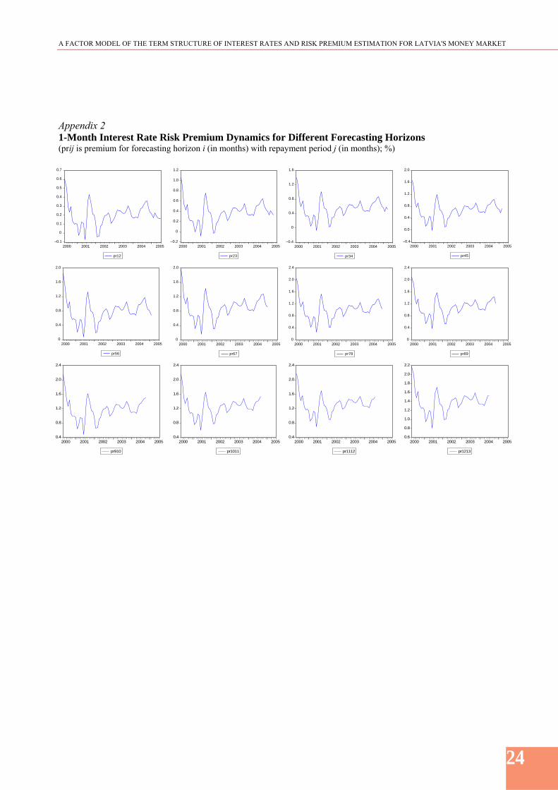
A FACTOR MODEL OF THE TERM STRUCTURE OF INTEREST RATES AND RISK PREMIUM ESTIMATION FOR LATVIAS MONEY MARKET
24
Appendix 2 1-Month Interest Rate Risk Premium Dynamics for Different Forecasting Horizons (prij is premium for forecasting horizon i (in months) with repayment period j (in months) )
04
08
12
16
20
24
2000 2001 2002 2003 2004 2005
pr910
04
08
12
16
20
24
2000 2001 2002 2003 2004 2005
pr1011
04
08
12
16
20
24
2000 2001 2002 2003 2004 2005
pr1112
06
08
10
12
14
16
18
20
22
2000 2001 2002 2003 2004 2005
pr1213
ndash01
0
01 02 03 04 05 06 07
2000 2001 2002 2003 2004 2005
p r 1 2 ndash02
0
02
04
06
08
10
12
2000 2001 2002 2003 2004 2005
pr23
ndash04
0
04
08
12
16
2000 2001 2002 2003 2004 2005 pr34
ndash04 00
04
08
12
16
20
2000 2001 2002 2003 2004 2005
pr45
0 04
08
12
16
20
2000 2001 2002 2003 2004 2005 p r 56
0
04
08
12
16
20
2000 2001 2002 2003 2004 2005
pr67
0
04
08
12
16
20
24
2000 2001 2002 2003 2004 2005 pr78
0
04
08
12
16
20
24
2000 2001 2002 2003 2004 2005
pr89
A FACTOR MODEL OF THE TERM STRUCTURE OF INTEREST RATES AND RISK PREMIUM ESTIMATION FOR LATVIAS MONEY MARKET
25
Appendix 3 3-Month Interest Rate Risk Premium Dynamics for Different Forecasting Horizons (prij is premium for forecasting horizon i (in months) with repayment period j (in months) )
00
04
08
12
16
20
2000 2001 2002 2003 2004 2005
pr58
04
08
12
16
20
2000 2001 2002 2003 2004 2005
pr912
04
06
08
10
12
14
16
18
20
2000 2001 2002 2003 2004 2005
pr1013
06
08
10
12
14
16
18
20
2000 2001 2002 2003 2004 2005
pr1114
06
08
10
12
14
16
18
20
2000 2001 2002 2003 2004 2005
pr1215
ndash01
0
01
02
03
04
05
06
2000 2001 2002 2003 2004 2005
p r 1 4 ndash02
0 02 04 06 08 10
2000 2001 2002 2003 2004 2005
pr25
0
02
04
06
08
10
12
14
2000 2001 2002 2003 2004 2005 pr36
0 02 04 06 08 10 12 14 16
2000 2001 2002 2003 2004 2005
pr47
0 04 08 12 16 20
2000 2001 2002 2003 2004 2005
pr811
0
04
08
12
16
20
2000 2001 2002 2003 2004 2005 pr710
0 04 08 12 16 20
2000 2001 2002 2003 2004 2005
pr69
ndash02
A FACTOR MODEL OF THE TERM STRUCTURE OF INTEREST RATES AND RISK PREMIUM ESTIMATION FOR LATVIAS MONEY MARKET
26
Appendix 4 6-Month Interest Rate Risk Premium Dynamics for Different Forecasting Horizons (prij is premium for forecasting horizon i (in months) with repayment period j (in months) )
02
04
06
08
10
12
14
16
2000 2001 2002 2003 2004 2005
pr612
02
04
06
08
10
12
14
16
2000 2001 2002 2003 2004 2005
pr713
02
04
06
08
10
12
14
16
18
2000 2001 2002 2003 2004 2005
pr814
04
06
08
10
12
14
16
18
2000 2001 2002 2003 2004 2005
pr915
04
06
08
10
12
14
16
18
2000 2001 2002 2003 2004 2005
pr1016
06
08
10
12
14
16
18
2000 2001 2002 2003 2004 2005
pr1117
06
08
10
12
14
16
18
2000 2001 2002 2003 2004 2005
pr1218
ndash01
0 01 02 03 04 05
2000 2001 2002 2003 2004 2005
pr 1 7ndash01
0
01
02
03
04
05
06
07
08
2000 2001 2002 2003 2004 2005
pr28
0
02
04
06
08
10
12
2000 2001 2002 2003 2004 2005
pr39
0 02 04 06 08 10 12 14
2000 2001 2002 2003 2004 2005
pr410
0 02
04
06
08
10
12
14
2000 2001 2002 2003 2004 2005
p r 5 1 1
A FACTOR MODEL OF THE TERM STRUCTURE OF INTEREST RATES AND RISK PREMIUM ESTIMATION FOR LATVIAS MONEY MARKET
27
Appendix 5 12-Month Interest Rate Risk Premium Dynamics for Different Forcasting Horizons (prij is premium for forecasting horizon i (in months) with repayment period j (in months) )
01
02
03
04
05
06
07
08
09
10
2000 2001 2002 2003 2004 2005
pr416
02
04
06
08
10
12
2000 2001 2002 2003 2004 2005
pr618
03
04
05
06
07
08
09
10
11
12
2000 2001 2002 2003 2004 2005
pr719
04
05
06
07
08
09
10
11
12
13
2000 2001 2002 2003 2004 2005
pr820
05
06
07
08
09
10
11
12
13
2000 2001 2002 2003 2004 2005
pr921
05
06
07
08
09
10
11
12
13
14
2000 2001 2002 2003 2004 2005
pr1022
06
07
08
09
10
11
12
13
14
2000 2001 2002 2003 2004 2005
pr1123
07
08
09
10
11
12
13
14
2000 2001 2002 2003 2004 2005
pr1224
ndash005
0 005
010
015
020
025
030
035
2000 2001 2002 2003 2004 2005
p r 11 3 0
01 02 03 04 05 06
2000 2001 2002 2003 2004 2005
pr214
0
01
02
03
04
05
06
07
08
2000 2001 2002 2003 2004 2005
pr315
0
02
04
06
08
10
12
2000 2001 2002 2003 2004 2005 pr 5 17
A FACTOR MODEL OF THE TERM STRUCTURE OF INTEREST RATES AND RISK PREMIUM ESTIMATION FOR LATVIAS MONEY MARKET
28
Appendix 6 Mean Interest Rate Risk Premium and Standard Deviation (prij is premium for forecasting horizon i (in months) with repayment period j (in months) ) On 1-month interest rate
pr12 pr23 pr34 pr45 pr56 pr67 pr78 pr89 pr910 pr1011 pr1112 pr1213 Mean premium 0193629 0364347 0515686 0650680 0771919 0881606 0981610 1073508 1158631 1238101 1312857 1383688Standard deviation 0124962 0211080 0267350 0300950 0317572 0321701 0316850 0305745 0290489 0272687 0253551 0233989
On 3-month interest rate
pr14 pr25 pr36 pr47 pr58 pr69 pr710 pr811 pr912 pr1013 pr1114 pr1215 Mean premium 0175572 0331301 0470243 0595022 0707878 0810715 0905146 0992536 1074034 1150609 1223071 1292104Standard deviation 0106270 0179455 0227233 0255724 0269783 0273233 0269068 0259613 0246660 0231579 0215408 0198923
On 6-month interest rate
pr17 pr28 pr39 pr410 pr511 pr612 pr713 pr814 pr915 pr1016 pr1117 pr1218 Mean premium 0154646 0293008 0417591 0530540 0633689 0728594 0816575 0898746 0976048 1049272 1119081 1186033Standard deviation 0084945 0143384 0181485 0204165 0215318 0218016 0214659 0207116 0196827 0184895 0172159 0159248
On 12-month interest rate
pr113 pr214 pr315 pr416 pr517 pr618 pr719 pr820 pr921 pr1022 pr1123 pr1224 Mean premium 0127464 0243277 0349219 0446817 0537372 0621988 0701603 0777008 0848869 0917749 0984119 1048375Standard deviation 0057915 0097684 0123556 0138914 0146443 0148255 0146006 0140985 0134193 0126398 0118191 0110020
A FACTOR MODEL OF THE TERM STRUCTURE OF INTEREST RATES AND RISK PREMIUM ESTIMATION FOR LATVIAS MONEY MARKET
29
BIBLIOGRAPHY 1 ANG Andrew PIAZZESI Monika A No-Arbitrage Vector Autoregression of Term Structure Dynamics with Macroeconomic and Latent Variables Journal of Monetary Economics vol 50 issue 4 May 2003 pp 745ndash787 2 CASSOLA Nuno LUIacuteS Barros Jorge A Two-factor Model of the German Term Structure of Interest Rates ECB Working Paper No 46 March 2001 3 CORTAZAR Gonzalo SCHWARTZ Eduardo S NARANJO Lorenzo Term Structure Estimation in Low-Frequency Transaction Markets A Kalman Filter Approach with Incomplete Panel-Data The Anderson School at UCLA Finance Working Paper No 6-03 2003 4 DIEBOLD Francis X LI Canlin Forecasting the Term Structure of Government Bond Yields NBER Working Paper No 10048 2003 5 DIEBOLD Francis X PIAZZESI Monika RUDEBUSCH Glenn D Modeling Bond Yields in Finance and Macroeconomics NBER Working Paper No 11089 2005 6 DIEBOLD Francis X RUDEBUSCH Glenn D ARUOBA Boragan S The Macroeconomy and the Yield Curve A Dynamic Latent Factor Approach NBER Working Paper No 10616 July 2004 7 DUFFEE Gregory R Term Premia and Interest Rate Forecasts in Affine Models Journal of Finance vol 57 No 1 February 2002 pp 405ndash443 8 DURREacute Alain EVJEN Snorre PILEGAARD Rasmus Estimating Risk Premia in Money Market Rates ECB Working Paper No 221 2003 9 EVANS Charles L MARSHALL David Monetary Policy and the Term Structure of Nominal Interest Rates Evidence and Theory Carnegie-Rochester Conference Series on Public Policy vol 49 1998 pp 53ndash111 10 EVANS Charles L MARSHALL David Economic Determinants of the Nominal Treasury Yield Curve Federal Reserve Bank of Chicago Working Papers No 16 2001 11 FRANKEL Jeffrey Alexander LOWN Cara S An Indicator of Future Inflation Extracted from the Steepness of the Interest Rate Yield Curve along its Entire Length Quarterly Journal of Economics vol 109 1994 pp 517ndash530 12 GRAVELLE Toni MULLER Philippe STREacuteLISKI David Towards a New Measure of Interest Rate Expectations in Canada Estimating a Time-Varying Term Premium Bank of Canada Proceedings of a Conference Information in Financial Asset Prices May 1998 13 HAMILTON James D Time Series Analysis Princeton University Press 1994 14 KENDALL Maurice G STUART Alan The Advanced Theory of Statistics London Griffin 1968 15 KNEZ Peter J LITTERMAN Robert SCHEINKMAN Joseacute Explorations into Factors Explaining Money Market Returns Journal of Finance vol 49 No 5 December 1994 pp 1861ndash1882 16 LITTERMAN Robert SCHEINKMAN Joseacute Common Factors Affecting Bond Returns Journal of Fixed Income vol 1 June 1991 pp 54ndash61
A FACTOR MODEL OF THE TERM STRUCTURE OF INTEREST RATES AND RISK PREMIUM ESTIMATION FOR LATVIAS MONEY MARKET
30
17 NELSON Charles R SIEGEL Andrew F Parsimonious Modeling of Yield Curves Journal of Business vol 60 1987 pp 473ndash489 18 SHILLER Robert J The Term Structure of Interest Rates B Friedman and F Hahn (eds) Handbook of Monetary Economics vol 1 Amsterdam North-Holland 1990 pp 627ndash722 19 The Stability-Oriented Monetary Policy Strategy of the Eurosystem ECB Monthly Bulletin No 1 January 1999 pp 39ndash505

A FACTOR MODEL OF THE TERM STRUCTURE OF INTEREST RATES AND RISK PREMIUM ESTIMATION FOR LATVIAS MONEY MARKET
25
Appendix 3 3-Month Interest Rate Risk Premium Dynamics for Different Forecasting Horizons (prij is premium for forecasting horizon i (in months) with repayment period j (in months) )
00
04
08
12
16
20
2000 2001 2002 2003 2004 2005
pr58
04
08
12
16
20
2000 2001 2002 2003 2004 2005
pr912
04
06
08
10
12
14
16
18
20
2000 2001 2002 2003 2004 2005
pr1013
06
08
10
12
14
16
18
20
2000 2001 2002 2003 2004 2005
pr1114
06
08
10
12
14
16
18
20
2000 2001 2002 2003 2004 2005
pr1215
ndash01
0
01
02
03
04
05
06
2000 2001 2002 2003 2004 2005
p r 1 4 ndash02
0 02 04 06 08 10
2000 2001 2002 2003 2004 2005
pr25
0
02
04
06
08
10
12
14
2000 2001 2002 2003 2004 2005 pr36
0 02 04 06 08 10 12 14 16
2000 2001 2002 2003 2004 2005
pr47
0 04 08 12 16 20
2000 2001 2002 2003 2004 2005
pr811
0
04
08
12
16
20
2000 2001 2002 2003 2004 2005 pr710
0 04 08 12 16 20
2000 2001 2002 2003 2004 2005
pr69
ndash02
A FACTOR MODEL OF THE TERM STRUCTURE OF INTEREST RATES AND RISK PREMIUM ESTIMATION FOR LATVIAS MONEY MARKET
26
Appendix 4 6-Month Interest Rate Risk Premium Dynamics for Different Forecasting Horizons (prij is premium for forecasting horizon i (in months) with repayment period j (in months) )
02
04
06
08
10
12
14
16
2000 2001 2002 2003 2004 2005
pr612
02
04
06
08
10
12
14
16
2000 2001 2002 2003 2004 2005
pr713
02
04
06
08
10
12
14
16
18
2000 2001 2002 2003 2004 2005
pr814
04
06
08
10
12
14
16
18
2000 2001 2002 2003 2004 2005
pr915
04
06
08
10
12
14
16
18
2000 2001 2002 2003 2004 2005
pr1016
06
08
10
12
14
16
18
2000 2001 2002 2003 2004 2005
pr1117
06
08
10
12
14
16
18
2000 2001 2002 2003 2004 2005
pr1218
ndash01
0 01 02 03 04 05
2000 2001 2002 2003 2004 2005
pr 1 7ndash01
0
01
02
03
04
05
06
07
08
2000 2001 2002 2003 2004 2005
pr28
0
02
04
06
08
10
12
2000 2001 2002 2003 2004 2005
pr39
0 02 04 06 08 10 12 14
2000 2001 2002 2003 2004 2005
pr410
0 02
04
06
08
10
12
14
2000 2001 2002 2003 2004 2005
p r 5 1 1
A FACTOR MODEL OF THE TERM STRUCTURE OF INTEREST RATES AND RISK PREMIUM ESTIMATION FOR LATVIAS MONEY MARKET
27
Appendix 5 12-Month Interest Rate Risk Premium Dynamics for Different Forcasting Horizons (prij is premium for forecasting horizon i (in months) with repayment period j (in months) )
01
02
03
04
05
06
07
08
09
10
2000 2001 2002 2003 2004 2005
pr416
02
04
06
08
10
12
2000 2001 2002 2003 2004 2005
pr618
03
04
05
06
07
08
09
10
11
12
2000 2001 2002 2003 2004 2005
pr719
04
05
06
07
08
09
10
11
12
13
2000 2001 2002 2003 2004 2005
pr820
05
06
07
08
09
10
11
12
13
2000 2001 2002 2003 2004 2005
pr921
05
06
07
08
09
10
11
12
13
14
2000 2001 2002 2003 2004 2005
pr1022
06
07
08
09
10
11
12
13
14
2000 2001 2002 2003 2004 2005
pr1123
07
08
09
10
11
12
13
14
2000 2001 2002 2003 2004 2005
pr1224
ndash005
0 005
010
015
020
025
030
035
2000 2001 2002 2003 2004 2005
p r 11 3 0
01 02 03 04 05 06
2000 2001 2002 2003 2004 2005
pr214
0
01
02
03
04
05
06
07
08
2000 2001 2002 2003 2004 2005
pr315
0
02
04
06
08
10
12
2000 2001 2002 2003 2004 2005 pr 5 17
A FACTOR MODEL OF THE TERM STRUCTURE OF INTEREST RATES AND RISK PREMIUM ESTIMATION FOR LATVIAS MONEY MARKET
28
Appendix 6 Mean Interest Rate Risk Premium and Standard Deviation (prij is premium for forecasting horizon i (in months) with repayment period j (in months) ) On 1-month interest rate
pr12 pr23 pr34 pr45 pr56 pr67 pr78 pr89 pr910 pr1011 pr1112 pr1213 Mean premium 0193629 0364347 0515686 0650680 0771919 0881606 0981610 1073508 1158631 1238101 1312857 1383688Standard deviation 0124962 0211080 0267350 0300950 0317572 0321701 0316850 0305745 0290489 0272687 0253551 0233989
On 3-month interest rate
pr14 pr25 pr36 pr47 pr58 pr69 pr710 pr811 pr912 pr1013 pr1114 pr1215 Mean premium 0175572 0331301 0470243 0595022 0707878 0810715 0905146 0992536 1074034 1150609 1223071 1292104Standard deviation 0106270 0179455 0227233 0255724 0269783 0273233 0269068 0259613 0246660 0231579 0215408 0198923
On 6-month interest rate
pr17 pr28 pr39 pr410 pr511 pr612 pr713 pr814 pr915 pr1016 pr1117 pr1218 Mean premium 0154646 0293008 0417591 0530540 0633689 0728594 0816575 0898746 0976048 1049272 1119081 1186033Standard deviation 0084945 0143384 0181485 0204165 0215318 0218016 0214659 0207116 0196827 0184895 0172159 0159248
On 12-month interest rate
pr113 pr214 pr315 pr416 pr517 pr618 pr719 pr820 pr921 pr1022 pr1123 pr1224 Mean premium 0127464 0243277 0349219 0446817 0537372 0621988 0701603 0777008 0848869 0917749 0984119 1048375Standard deviation 0057915 0097684 0123556 0138914 0146443 0148255 0146006 0140985 0134193 0126398 0118191 0110020
A FACTOR MODEL OF THE TERM STRUCTURE OF INTEREST RATES AND RISK PREMIUM ESTIMATION FOR LATVIAS MONEY MARKET
29
BIBLIOGRAPHY 1 ANG Andrew PIAZZESI Monika A No-Arbitrage Vector Autoregression of Term Structure Dynamics with Macroeconomic and Latent Variables Journal of Monetary Economics vol 50 issue 4 May 2003 pp 745ndash787 2 CASSOLA Nuno LUIacuteS Barros Jorge A Two-factor Model of the German Term Structure of Interest Rates ECB Working Paper No 46 March 2001 3 CORTAZAR Gonzalo SCHWARTZ Eduardo S NARANJO Lorenzo Term Structure Estimation in Low-Frequency Transaction Markets A Kalman Filter Approach with Incomplete Panel-Data The Anderson School at UCLA Finance Working Paper No 6-03 2003 4 DIEBOLD Francis X LI Canlin Forecasting the Term Structure of Government Bond Yields NBER Working Paper No 10048 2003 5 DIEBOLD Francis X PIAZZESI Monika RUDEBUSCH Glenn D Modeling Bond Yields in Finance and Macroeconomics NBER Working Paper No 11089 2005 6 DIEBOLD Francis X RUDEBUSCH Glenn D ARUOBA Boragan S The Macroeconomy and the Yield Curve A Dynamic Latent Factor Approach NBER Working Paper No 10616 July 2004 7 DUFFEE Gregory R Term Premia and Interest Rate Forecasts in Affine Models Journal of Finance vol 57 No 1 February 2002 pp 405ndash443 8 DURREacute Alain EVJEN Snorre PILEGAARD Rasmus Estimating Risk Premia in Money Market Rates ECB Working Paper No 221 2003 9 EVANS Charles L MARSHALL David Monetary Policy and the Term Structure of Nominal Interest Rates Evidence and Theory Carnegie-Rochester Conference Series on Public Policy vol 49 1998 pp 53ndash111 10 EVANS Charles L MARSHALL David Economic Determinants of the Nominal Treasury Yield Curve Federal Reserve Bank of Chicago Working Papers No 16 2001 11 FRANKEL Jeffrey Alexander LOWN Cara S An Indicator of Future Inflation Extracted from the Steepness of the Interest Rate Yield Curve along its Entire Length Quarterly Journal of Economics vol 109 1994 pp 517ndash530 12 GRAVELLE Toni MULLER Philippe STREacuteLISKI David Towards a New Measure of Interest Rate Expectations in Canada Estimating a Time-Varying Term Premium Bank of Canada Proceedings of a Conference Information in Financial Asset Prices May 1998 13 HAMILTON James D Time Series Analysis Princeton University Press 1994 14 KENDALL Maurice G STUART Alan The Advanced Theory of Statistics London Griffin 1968 15 KNEZ Peter J LITTERMAN Robert SCHEINKMAN Joseacute Explorations into Factors Explaining Money Market Returns Journal of Finance vol 49 No 5 December 1994 pp 1861ndash1882 16 LITTERMAN Robert SCHEINKMAN Joseacute Common Factors Affecting Bond Returns Journal of Fixed Income vol 1 June 1991 pp 54ndash61
A FACTOR MODEL OF THE TERM STRUCTURE OF INTEREST RATES AND RISK PREMIUM ESTIMATION FOR LATVIAS MONEY MARKET
30
17 NELSON Charles R SIEGEL Andrew F Parsimonious Modeling of Yield Curves Journal of Business vol 60 1987 pp 473ndash489 18 SHILLER Robert J The Term Structure of Interest Rates B Friedman and F Hahn (eds) Handbook of Monetary Economics vol 1 Amsterdam North-Holland 1990 pp 627ndash722 19 The Stability-Oriented Monetary Policy Strategy of the Eurosystem ECB Monthly Bulletin No 1 January 1999 pp 39ndash505
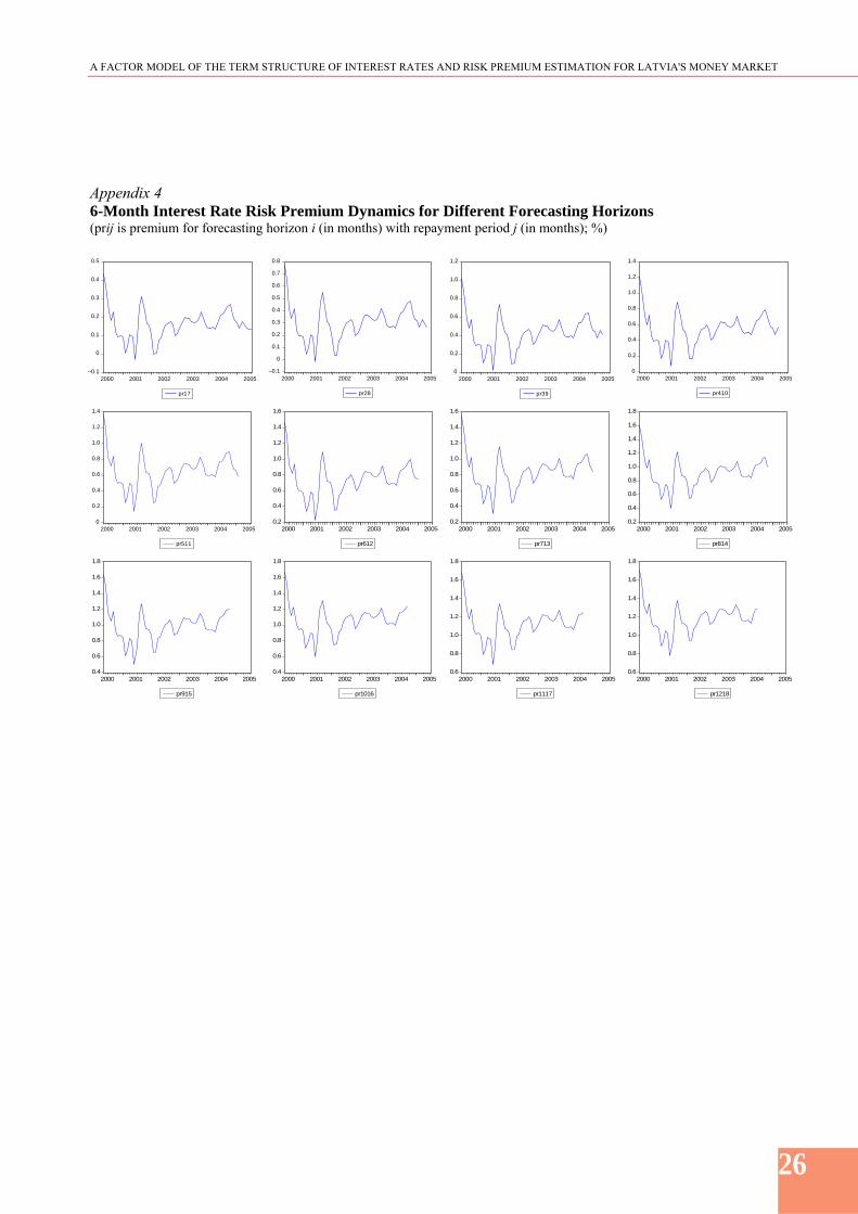
A FACTOR MODEL OF THE TERM STRUCTURE OF INTEREST RATES AND RISK PREMIUM ESTIMATION FOR LATVIAS MONEY MARKET
26
Appendix 4 6-Month Interest Rate Risk Premium Dynamics for Different Forecasting Horizons (prij is premium for forecasting horizon i (in months) with repayment period j (in months) )
02
04
06
08
10
12
14
16
2000 2001 2002 2003 2004 2005
pr612
02
04
06
08
10
12
14
16
2000 2001 2002 2003 2004 2005
pr713
02
04
06
08
10
12
14
16
18
2000 2001 2002 2003 2004 2005
pr814
04
06
08
10
12
14
16
18
2000 2001 2002 2003 2004 2005
pr915
04
06
08
10
12
14
16
18
2000 2001 2002 2003 2004 2005
pr1016
06
08
10
12
14
16
18
2000 2001 2002 2003 2004 2005
pr1117
06
08
10
12
14
16
18
2000 2001 2002 2003 2004 2005
pr1218
ndash01
0 01 02 03 04 05
2000 2001 2002 2003 2004 2005
pr 1 7ndash01
0
01
02
03
04
05
06
07
08
2000 2001 2002 2003 2004 2005
pr28
0
02
04
06
08
10
12
2000 2001 2002 2003 2004 2005
pr39
0 02 04 06 08 10 12 14
2000 2001 2002 2003 2004 2005
pr410
0 02
04
06
08
10
12
14
2000 2001 2002 2003 2004 2005
p r 5 1 1
A FACTOR MODEL OF THE TERM STRUCTURE OF INTEREST RATES AND RISK PREMIUM ESTIMATION FOR LATVIAS MONEY MARKET
27
Appendix 5 12-Month Interest Rate Risk Premium Dynamics for Different Forcasting Horizons (prij is premium for forecasting horizon i (in months) with repayment period j (in months) )
01
02
03
04
05
06
07
08
09
10
2000 2001 2002 2003 2004 2005
pr416
02
04
06
08
10
12
2000 2001 2002 2003 2004 2005
pr618
03
04
05
06
07
08
09
10
11
12
2000 2001 2002 2003 2004 2005
pr719
04
05
06
07
08
09
10
11
12
13
2000 2001 2002 2003 2004 2005
pr820
05
06
07
08
09
10
11
12
13
2000 2001 2002 2003 2004 2005
pr921
05
06
07
08
09
10
11
12
13
14
2000 2001 2002 2003 2004 2005
pr1022
06
07
08
09
10
11
12
13
14
2000 2001 2002 2003 2004 2005
pr1123
07
08
09
10
11
12
13
14
2000 2001 2002 2003 2004 2005
pr1224
ndash005
0 005
010
015
020
025
030
035
2000 2001 2002 2003 2004 2005
p r 11 3 0
01 02 03 04 05 06
2000 2001 2002 2003 2004 2005
pr214
0
01
02
03
04
05
06
07
08
2000 2001 2002 2003 2004 2005
pr315
0
02
04
06
08
10
12
2000 2001 2002 2003 2004 2005 pr 5 17
A FACTOR MODEL OF THE TERM STRUCTURE OF INTEREST RATES AND RISK PREMIUM ESTIMATION FOR LATVIAS MONEY MARKET
28
Appendix 6 Mean Interest Rate Risk Premium and Standard Deviation (prij is premium for forecasting horizon i (in months) with repayment period j (in months) ) On 1-month interest rate
pr12 pr23 pr34 pr45 pr56 pr67 pr78 pr89 pr910 pr1011 pr1112 pr1213 Mean premium 0193629 0364347 0515686 0650680 0771919 0881606 0981610 1073508 1158631 1238101 1312857 1383688Standard deviation 0124962 0211080 0267350 0300950 0317572 0321701 0316850 0305745 0290489 0272687 0253551 0233989
On 3-month interest rate
pr14 pr25 pr36 pr47 pr58 pr69 pr710 pr811 pr912 pr1013 pr1114 pr1215 Mean premium 0175572 0331301 0470243 0595022 0707878 0810715 0905146 0992536 1074034 1150609 1223071 1292104Standard deviation 0106270 0179455 0227233 0255724 0269783 0273233 0269068 0259613 0246660 0231579 0215408 0198923
On 6-month interest rate
pr17 pr28 pr39 pr410 pr511 pr612 pr713 pr814 pr915 pr1016 pr1117 pr1218 Mean premium 0154646 0293008 0417591 0530540 0633689 0728594 0816575 0898746 0976048 1049272 1119081 1186033Standard deviation 0084945 0143384 0181485 0204165 0215318 0218016 0214659 0207116 0196827 0184895 0172159 0159248
On 12-month interest rate
pr113 pr214 pr315 pr416 pr517 pr618 pr719 pr820 pr921 pr1022 pr1123 pr1224 Mean premium 0127464 0243277 0349219 0446817 0537372 0621988 0701603 0777008 0848869 0917749 0984119 1048375Standard deviation 0057915 0097684 0123556 0138914 0146443 0148255 0146006 0140985 0134193 0126398 0118191 0110020
A FACTOR MODEL OF THE TERM STRUCTURE OF INTEREST RATES AND RISK PREMIUM ESTIMATION FOR LATVIAS MONEY MARKET
29
BIBLIOGRAPHY 1 ANG Andrew PIAZZESI Monika A No-Arbitrage Vector Autoregression of Term Structure Dynamics with Macroeconomic and Latent Variables Journal of Monetary Economics vol 50 issue 4 May 2003 pp 745ndash787 2 CASSOLA Nuno LUIacuteS Barros Jorge A Two-factor Model of the German Term Structure of Interest Rates ECB Working Paper No 46 March 2001 3 CORTAZAR Gonzalo SCHWARTZ Eduardo S NARANJO Lorenzo Term Structure Estimation in Low-Frequency Transaction Markets A Kalman Filter Approach with Incomplete Panel-Data The Anderson School at UCLA Finance Working Paper No 6-03 2003 4 DIEBOLD Francis X LI Canlin Forecasting the Term Structure of Government Bond Yields NBER Working Paper No 10048 2003 5 DIEBOLD Francis X PIAZZESI Monika RUDEBUSCH Glenn D Modeling Bond Yields in Finance and Macroeconomics NBER Working Paper No 11089 2005 6 DIEBOLD Francis X RUDEBUSCH Glenn D ARUOBA Boragan S The Macroeconomy and the Yield Curve A Dynamic Latent Factor Approach NBER Working Paper No 10616 July 2004 7 DUFFEE Gregory R Term Premia and Interest Rate Forecasts in Affine Models Journal of Finance vol 57 No 1 February 2002 pp 405ndash443 8 DURREacute Alain EVJEN Snorre PILEGAARD Rasmus Estimating Risk Premia in Money Market Rates ECB Working Paper No 221 2003 9 EVANS Charles L MARSHALL David Monetary Policy and the Term Structure of Nominal Interest Rates Evidence and Theory Carnegie-Rochester Conference Series on Public Policy vol 49 1998 pp 53ndash111 10 EVANS Charles L MARSHALL David Economic Determinants of the Nominal Treasury Yield Curve Federal Reserve Bank of Chicago Working Papers No 16 2001 11 FRANKEL Jeffrey Alexander LOWN Cara S An Indicator of Future Inflation Extracted from the Steepness of the Interest Rate Yield Curve along its Entire Length Quarterly Journal of Economics vol 109 1994 pp 517ndash530 12 GRAVELLE Toni MULLER Philippe STREacuteLISKI David Towards a New Measure of Interest Rate Expectations in Canada Estimating a Time-Varying Term Premium Bank of Canada Proceedings of a Conference Information in Financial Asset Prices May 1998 13 HAMILTON James D Time Series Analysis Princeton University Press 1994 14 KENDALL Maurice G STUART Alan The Advanced Theory of Statistics London Griffin 1968 15 KNEZ Peter J LITTERMAN Robert SCHEINKMAN Joseacute Explorations into Factors Explaining Money Market Returns Journal of Finance vol 49 No 5 December 1994 pp 1861ndash1882 16 LITTERMAN Robert SCHEINKMAN Joseacute Common Factors Affecting Bond Returns Journal of Fixed Income vol 1 June 1991 pp 54ndash61
A FACTOR MODEL OF THE TERM STRUCTURE OF INTEREST RATES AND RISK PREMIUM ESTIMATION FOR LATVIAS MONEY MARKET
30
17 NELSON Charles R SIEGEL Andrew F Parsimonious Modeling of Yield Curves Journal of Business vol 60 1987 pp 473ndash489 18 SHILLER Robert J The Term Structure of Interest Rates B Friedman and F Hahn (eds) Handbook of Monetary Economics vol 1 Amsterdam North-Holland 1990 pp 627ndash722 19 The Stability-Oriented Monetary Policy Strategy of the Eurosystem ECB Monthly Bulletin No 1 January 1999 pp 39ndash505
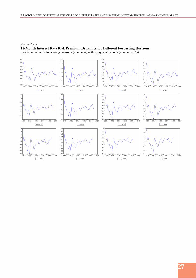
A FACTOR MODEL OF THE TERM STRUCTURE OF INTEREST RATES AND RISK PREMIUM ESTIMATION FOR LATVIAS MONEY MARKET
30
17 NELSON Charles R SIEGEL Andrew F Parsimonious Modeling of Yield Curves Journal of Business vol 60 1987 pp 473ndash489 18 SHILLER Robert J The Term Structure of Interest Rates B Friedman and F Hahn (eds) Handbook of Monetary Economics vol 1 Amsterdam North-Holland 1990 pp 627ndash722 19 The Stability-Oriented Monetary Policy Strategy of the Eurosystem ECB Monthly Bulletin No 1 January 1999 pp 39ndash505