A dynamic theory of war and peace - Columbia … dynamic theory of war ... we apply the modern tools...

Journal of Economic Theory 145 (2010) 1921–1950

www.elsevier.com/locate/jet

A dynamic theory of war and peace ✩

Pierre Yared ∗

Columbia University, Graduate School of Business, Uris Hall, 3022 Broadway, New York, NY 10027, United States

Received 16 January 2009; final version received 26 August 2009; accepted 8 March 2010

Available online 10 May 2010

Abstract

In every period, an aggressive country seeks concessions from a non-aggressive country with privateinformation about their cost. The aggressive country can force concessions via war, and both countries sufferfrom limited commitment. We characterize the efficient sequential equilibria. We show that war is necessaryto sustain peace and that temporary wars can emerge because of the coarseness of public information. Inthe long run, temporary wars can be sustained only if countries are patient, if the cost of war is large, and ifthe cost of concessions is low.© 2010 Elsevier Inc. All rights reserved.

JEL classification: D82; D86; F5; N4

Keywords: Asymmetric and private information; Contract theory; International political economy; War

1. Introduction

The subject of war, first formalized in an economic framework in the seminal work ofSchelling [34] and Aumann and Maschler [5], is the original impetus for important advances inthe field of game theory. While there is renewed theoretical interest in the subject of war in eco-nomics, no formal framework exists for investigating the transitional dynamics between war and

✩ I am especially grateful to Daron Acemoglu and to Mike Golosov for their support and encouragement. I wouldalso like to thank Stefania Albanesi, Andrew Atkeson, V.V. Chari, Sylvain Chassang, Alexandre Debs, Oeindrila Dube,Roozbeh Hosseini, Larry Jones, Patrick Kehoe, Narayana Kocherlakota, David Laitin, Gerard Padró i Miquel, SantiagoOliveros, Christopher Phelan, Robert Powell, Debraj Ray, Dmitriy Sergeyev, Aleh Tsyvinski, Ivan Werning, and threeanonymous referees for comments. This paper replaces a previous version which circulated under the title “A DynamicTheory of Concessions and War.”

* Fax: +1 212 662 8474.E-mail address: [email protected].

0022-0531/$ – see front matter © 2010 Elsevier Inc. All rights reserved.doi:10.1016/j.jet.2010.04.005

1922 P. Yared / Journal of Economic Theory 145 (2010) 1921–1950

peace.1 In this paper, we apply the modern tools from the theory of repeated games developedby Abreu, Pearce, and Stacchetti [2,3] to the classical subject of war. Specifically, we presenta dynamic theory of war in which countries suffer from limited commitment and asymmetricinformation, two frictions which hamper their ability to peacefully negotiate. Our main concep-tual result is a dynamic theory of escalation, temporary wars, and total war. On the theoreticalside, our framework additionally allows us to derive novel results on the role of information inrepeated games and dynamic contracts.2

In our model, one country, which we refer to as the aggressive country, is dissatisfied withthe status quo and seeks concessions from its rival, which we refer to as the non-aggressivecountry. In every period, the aggressive country can either forcibly extract these concessions viawar, or it can let the non-aggressive country peacefully make the concessions on its own. Whilepeaceful concession-making is clearly less destructive than war, there are two limitations on theextent to which peaceful bargaining is possible. First, there is limited commitment. Specifically,the non-aggressive country cannot commit to making a concession once it sees that the threatof war has subsided. Moreover, the aggressive country cannot commit to peace in the futurein order to reward concession-making by the non-aggressive country today. Second, there isimperfect information. The aggressive country does not have any information regarding the non-aggressive country’s ability to make a concession, and the non-aggressive country can use thisto its advantage. Specifically, since there is always a positive probability that concessions are toocostly to make, the non-aggressive country may wish to misrepresent itself as being unable tomake a concession whenever it is actually able to do so.

There are many applications of our framework. As an example, consider the events whichpreceded the First Barbary War (1801–1805) which are described in detail in Lambert [25].The Barbary States of North Africa (the aggressive country) requested tribute from the UnitedStates (the non-aggressive country) in exchange for the safe passage of American ships throughthe Mediterranean. The United States failed to make successful payments on multiple occa-sions, in part because of the small size of the government budget relative to the requested tributeand because of resistance from Congress. This resulted in the Pacha of Tripoli requesting ever-increasing concessions. Eventually, failure to make concessions resulted in the First Barbary Warwhich culminated with the partial forgiveness of past American debts and a continuation of thepeaceful relationship between the Barbary States and the United States. Eventually, however, theUnited States continued to miss payments, and this resulted in the Second Barbary War (1815)from which the United States emerged victorious and which ended the Mediterranean tributesystem. This historical episode highlights how limited commitment to peace and to concessionstogether with imperfect information about the cost of concessions can lead to war.

We use our framework to consider the efficient sequential equilibria in which countries followhistory-dependent strategies so as to characterize the rich dynamic path of war and peace. In ourcharacterization, we distinguish between temporary war and total war, defining the latter as thepermanent realization of war and the absence of negotiation. In our model, war is the uniquestatic Nash equilibrium, so that total war is equivalent to the repeated static Nash equilibrium inwhich countries refrain from ever peacefully negotiating.

Our paper presents three main results. Our first result is that wars are necessary along theequilibrium path. This insight adds to the theory of war by showing how the realization of war

1 Examples of recent papers on war include but are by no means limited to [7,9–12,14,15,22–24,26,28,29,35,36].2 Our theoretical framework is very close to applied models of dynamic optimal contracts with private information

(e.g., [6,19,21,27,37,38]).

P. Yared / Journal of Economic Theory 145 (2010) 1921–1950 1923

serves as a punishment for the failure to engage in successful peaceful bargaining in the past.In our framework, both the aggressive and non-aggressive country recognize that war is ex-postinefficient, though it improves ex-ante efficiency by providing incentives for concession-makingby the non-aggressive country. Our intuition for the realization of war is linked to the insightsachieved by previous work on the theory of repeated games which shows that the realizationof inefficient outcomes (such as price wars) can sustain efficient outcomes along the equilibriumpath (e.g., [2,3,20,30]). An important technical distinction of our work from this theoretical workis that information in our environment is coarse. Specifically, though the aggressive country isalways certain that the non-aggressive country is cooperating whenever concessions succeed, theaggressive country receives no information if concessions fail, and it cannot deduce the likelihoodthat the non-aggressive country is genuinely unable to make a concession. Therefore, there is achance that the aggressive country is making a mistake by going to war. This technical distinctionis important for our next results.

Our second result is that temporary war can occur along the equilibrium path. While the ag-gressive country must fight the non-aggressive country in order to sustain concessions, it neednot engage in total war; it can forgive the non-aggressive country for the first few failed conces-sions by providing the non-aggressive country with another chance at peace after the first roundof fighting. This insight emerges because of the coarseness of information in our environment.There is a large chance that the aggressive country is misinterpreting the failure to make a con-cession as being due to lack of cooperation. Consequently, even though it is efficient for theaggressive country to punish initial failed concessions with the most extreme punishment of totalwar, this is not necessary for efficiency since it may be making an error. More specifically, theequilibrium begins in the following fashion: Periods of peace are marked by escalating demandsin which failure to make concessions by the non-aggressive country leads the aggressive countryto request bigger and bigger concessions. Both countries strictly prefer this scenario to one inwhich initial failures to make a concession are punished by war since war is destructive and rep-resents a welfare loss for both countries. With positive probability, the non-aggressive country isincapable of making concessions for several periods in sequence so that requested concessionsbecome larger and larger, and the only way for the aggressive country to provide incentives forsuch large concessions to be made is to fight the non-aggressive country if these concessions fail.Consequently, some initial concessions fail, war takes place, and this war may culminate withthe aggressive country forgiving the non-aggressive country and giving peace another chance.

Our final result is that countries can engage in temporary wars in the long run only underspecial conditions, and countries necessarily converge to total war if these conditions are notsatisfied. More specifically, temporary wars can be sustained in the long run equilibrium if coun-tries are sufficiently patient, if the cost of war is sufficiently large, and if cost of concessions issufficiently low. If countries are patient and if war is very costly relative to peace, then total waris an extremely costly punishment which need not be exercised to elicit peaceful concessions,particularly since these are not so costly for the non-aggressive country to make. In the longrun, no matter how many concessions fail, the aggressive country can continue to forgive thenon-aggressive country after a round of fighting and to provide the non-aggressive country withanother chance at peace. In contrast, if countries are impatient, if the cost of war is low, or if thecost of making concessions is high, then countries must converge to total war. In this scenario,even the most extreme punishment of total war is not unpleasant enough for the non-aggressivecountry since it does not suffer so much under war and it does not place much value on the future.Moreover, the cost of making a peaceful concession for the non-aggressive country is so largethat it eventually requires an extreme punishment for failure to meet its obligation. Consequently,


even though temporary wars can occur along the equilibrium path through the process of escalat-ing demands, eventually it becomes impossible for the aggressive country to continue to forgivethe non-aggressive country and total war becomes a necessity.

Our paper makes two contributions. First, it is an application of a repeated imperfect informa-tion game with history-dependent strategies to war. This is important since the study of war is adynamic issue in which countries have long memories — particularly in long-lasting conflicts —and since the literature on war has recognized the importance of limited commitment and imper-fect information. In contrast to the current work on war, we provide an explanation for war whichcombines these two frictions in a dynamic setting in which countries follow history-dependentstrategies and in which neither peace nor war is an absorbing state. This allows the model tofeature escalating demands, temporary wars, and total war.3

Second, our paper is an application of a repeated imperfect information game in an environ-ment with a coarse information structure. Much of the existing literature on repeated games anddynamic contracts assumes a rich information structure, and this leads to the necessity of theBang–Bang characterization of efficient equilibria.4 In the context of war and diplomacy, thisinformation structure and its equilibrium implications may not be appropriate. First, countriesoften have very little information about their enemy’s behavior and intentions, particularly whentheir enemy is not cooperating. Second, even though temporary wars occur in actuality, in manyenvironments in which total war represents the worst possible outcome, the Bang–Bang charac-terization of efficient equilibria implies that temporary wars do not occur.5 In this paper, we showthat under a coarse information structure, the Bang–Bang property is not necessary for efficiencysince the prospect for error is large, and this allows us to generate temporary wars in equilib-rium. Nevertheless, we show that the Bang–Bang property must hold in the long run under someconditions in which countries converge to total war.6

The paper is organized as follows. Section 2 describes the model. Section 3 defines efficientsequential equilibria. Section 4 characterizes the equilibrium and provides our main results. Sec-tion 5 concludes. Appendix A contains all proofs and additional material not included in thetext.

2. Model

We consider an environment in which an aggressive country seeks political or economic con-cessions from a non-aggressive country.7 In every period, the aggressive country can enforcethese concessions by war, or it can let the non-aggressive country make these concessions uni-laterally under peace. With some positive probability, the non-aggressive country is incapableof making concessions because they are too costly. This may happen, for instance, becausethe non-aggressive country’s government experiences severe domestic opposition to concession-

3 In addition to the work discussed in footnote 1, our work is also related to the model of Acemoglu and Robinson [4]on conflict and regime change, though they do not consider the role of asymmetric information.

4 This literature is large and cannot be summarized here. See for example [2,3,18,31,32].5 That is if total war is the min–max. This characterization applies only to efficient equilibria. Efficient equilibria

as opposed to other often-examined equilibria such as Markovian equilibria or trigger strategy equilibria are a usefulselection device in our setting since rival countries have long memories of their past interactions which can lead toescalation.

6 See [17,33] for an additional discussion of the characteristics of equilibria under different information structures.7 While we frame our discussion with respect to two countries, the insights from this model can apply to groups within

countries.


Fig. 1. Game.

making. Nevertheless, this cost of concession-making is not observed by the aggressive country,so that the non-aggressive country can always lie about the true reasons for the failure of conces-sions.

More formally, there are two countries i = {1,2} and time periods t = {0, . . . ,∞}. Country 1is the aggressive country and country 2 is the non-aggressive country. In every date t , country 1publicly chooses Wt = {0,1}. If Wt = 1, war takes place, each country i receives wi , and theperiod ends. Alternatively, if Wt = 0, peace occurs, and country 2 publicly makes a concessionto country 1 of size xt ∈ [0, x]. Country 1 receives xt and country 2 receives −xt − c(xt , st ) forc(xt , st ) which represents country 2’s private additional cost of making a concession xt which is afunction of the state st = {0,1}. st is observed by country 2 but not by country 1. Let c(xt , st ) =c > 0 if xt > 0 and st = 0 and let c(xt , st ) = 0 otherwise. st is stochastic and determined asfollows. If Wt = 0, then prior to the choice of xt , nature chooses st with Pr{st = 1} = π ∈ (0,1).

Concessions by country 2 are more costly if st = 0, but this cannot be verified by country 1.For example, suppose that c is very high — as we will do — and suppose this implies thatconcessions cannot be positive if st = 0. Then, if Wt = 0 and if country 1 receives no concessions(i.e., xt = 0), country 1 cannot tell if country 2 could not make concessions since the cost wastoo high (i.e., st = 0) or if country 2 could make concessions but chose to not cooperate (i.e.,st = 1).

We do not allow country 2 to choose to go to war or to receive concessions from country 1 onlyas a matter of parsimony. Under this additional refinement, the characterization of the equilibriumis identical to the one presented here, and all of our results are left unchanged.8 Moreover, allof our results and intuitions generalize to an environment in which concessions are binary withxt ∈ {0, x}.9 The game is displayed in Fig. 1.

8 Such a model is isomorphic to the one here since country 1 always makes zero concessions. Details available uponrequest.

9 This may be more appropriate for some applications. Details available upon request.


Let ui(Wt , xt , st ) represent the payoff to i at t .10 Each country i has a period zero welfare

E0

∞∑t=0

βtui(Wt , xt , st ), β ∈ (0,1).

Assumption 1 (Inefficiency of war). ∃x ∈ [0, x] s.t. πx > w1 and −πx > w2.

Assumption 2 (Military power of country 1). w1 > 0.

Assumption 1 captures the fact that war is destructive, since both countries can be madebetter off if war does not take place and country 2 makes a concession to country 1 in state 1.Assumption 2 illustrates why country 1 is the aggressive country, since country 1’s militarypower w1 exceeds the economic resources under its control of size 0. The fact that w1 exceedsw2 (which is negative) is without loss of generality, and it is due to the normalization of bothcountries’ resources to 0 which is purely for notational simplicity.11

Assumption 2 has an important implication. Specifically, in a one-shot equilibrium W = 1 isthe unique static Nash equilibrium. This is because conditional on W = 0, country 2 choosesx = 0. Thus, by Assumption 2, country 1 chooses W = 1. Because the possibility of war pre-cedes the possibility of peace, country 2 cannot commit to making concessions.12 Consequently,in a static equilibrium, country 1, which is dissatisfied with the lack of concessions (by Assump-tion 2), will choose to enforce concessions via war rather than to provide country 2 with a chanceat peace.

Since the static Nash equilibrium is inefficient (by Assumption 1), one can imagine that in adynamic framework, country 1 may be able to enforce concessions from country 2 by rewardingsuccessful concessions today by refraining from war in the future. Nevertheless, there are twoobstacles to this arrangement which are important to consider. First, country 1 cannot commit tounconditionally refraining from war in the future, since it also suffers from limited commitment.Thus, whenever country 1 refrains from fighting at some date, it must be promised sufficientconcessions in the future as a reward. Second, country 1 does not observe the state st and thecost of concessions c(·,·) which may be very large.

Assumption 3 (High cost of concessions). c > −βw2/(1 − β).

In a dynamic environment, Assumption 3 implies that if st = 0, then country 2’s concessionsare so prohibitively costly that even the highest reward for a positive concession and the highestpunishment for zero concessions together cannot induce a positive concession by country 2.13

Therefore, concessions must be zero if st = 0. Consequently, if concessions fail (i.e., xt = 0),country 1 cannot determine if this is unintentional because their cost is too high (i.e., st = 0) or

10 Specifically, u1(Wt , xt , st ) = Wtw1 + (1 − Wt )xt and u2(Wt , xt , st ) = Wtw2 − (1 − Wt )(xt + c(xt , st )).11 Country 2 can be more powerful and control more resources than country 1 and vice versa as long as country 1’smilitary power exceeds its economic power. More generally, wi can emerge from a possibly costly and unfair lotteryover a set of resources.12 The fact that the opportunity to engage in war precedes the opportunity to engage in negotiations is important forthe interpretation of dynamics since every period features either war or negotiations. This also captures the fact thatnegotiations are costly for country 1 since it forgoes the opportunity of war.13 This is because the discounted difference between the largest possible reward (permanent peace with continuationvalue of 0) and the largest possible punishment (permanent war with continuation value of w2/(1−β)) is not sufficientlylarge relative to c.


if this is intentional because their cost is low (i.e., st = 1). This means that if country 1 goes towar in response to a failed concession, there is a chance that it is making a mistake since theconcession’s failure is unintentional.14

More formally, information in our environment is coarse. Though country 1 is always certainthat country 2 is cooperating whenever concessions succeed, country 1 receives no information ifconcessions fail, and it cannot deduce the likelihood that country 2 is genuinely unable to make aconcession. As we will discuss in Section 4.2, this detail is important as it will lead to temporarywars.

3. Efficient sequential equilibria

In this section, we formally define the equilibrium and we present our recursive method forthe characterization of the efficient sequential equilibria between the two countries.

3.1. Equilibrium definition

We begin by formally defining randomization since we allow countries to play correlatedstrategies. Let zt ∈ [0,1] represent an i.i.d. random variable independent of st and all actionswhich is drawn from a uniform c.d.f. G(·) at the beginning of every period t . zt is observedby both countries and can be used as a randomization device which can improve efficiency byallowing country 1 to probabilistically go to war.

We consider equilibria in which each country conditions its strategy on past public informa-tion. Let ht = {zt−1,W t−1, xt−1}, the history of public information at t prior to the realizationof zt .15 Define a strategy σ = {σ1, σ2} = {{Wt(ht , zt )}∞t=0, {{xt (ht , zt , st )}st=0,1}∞t=0}. σ is feasi-ble if ∀t � 0 and ∀(ht , zt ),{

Wt(ht , zt ),{xt (ht , zt , st )

}st=0,1

} ∈ {{0,1}, [0, x]2}.Given σ , define the equilibrium continuation value for country i at (ht , zt ) as

Ui(σ |ht ,zt ) = E{ui

(Wt(ht , zt ), xt (ht , zt , st ), st

)+ βE

{Ui(σ |ht+1,zt+1)

∣∣ ht , zt ,Wt (ht , zt ), xt (ht , zt , st )} ∣∣ ht , zt

}(1)

for σ |ht ,zt which is the continuation of a strategy after (ht , zt ) has been realized. Let Ui(σ |ht ,zt )|stcorrespond to the object inside the first expectations operator in (1) and let Σi |ht ,zt denote theentire set of feasible continuation strategies for i after (ht , zt ) has been realized.

Definition 1. σ is a sequential equilibrium if it is feasible and if ∀(ht , zt )

U1(σ |ht ,zt ) � U1(σ ′

1|ht ,zt , σ2|ht ,zt

) ∀σ ′1|ht ,zt ∈ Σ1|ht ,zt , and

U2(σ |ht ,zt )|st � U2(σ1|ht ,zt , σ

′2|ht ,zt

)|st ∀σ ′2|ht ,zt ∈ Σ2|ht ,zt and st = {0,1}.

In a sequential equilibrium, each country dynamically chooses its best response given thestrategy of its rival. The definition takes into account that country 1’s actions are chosen at (ht , zt )

14 One can interpret our model as a reduced-form representation of an environment in which a stochastic surplus onlyobservable to and controlled by country 2 must be divided. This surplus is zero if st = 0 and positive if st = 1. Thecommitment problem arises because the surplus is divided after the possibility of war.15 Without loss of generality, we let xt = 0 if Wt = 1.


whereas country 2’s actions are chosen at (ht , zt , st ). Because country 1’s strategy is public bydefinition, any deviation by country 2 to a non-public strategy is irrelevant (see [18]).

In order to build a sequential equilibrium allocation which is generated by a particular strategy,let qt = {zt−1, st−1}, the exogenous equilibrium history of public signals and states prior to therealization of zt .16 Define an equilibrium allocation as a function of the exogenous history:

α = {Wt(qt , zt ),

{xt (qt , zt , st )

}}∞t=0.

Let F denote the set of feasible allocations α with continuation allocations from t onwardwhich are measurable with respect to public information generated up to t . Let Ui(α|qt ,zt ) corre-spond to country i’s continuation value at t conditional on (qt , zt ). Finally, define

Ui = wi

1 − β,

the payoff from the repeated static Nash equilibrium. Because the repeated static Nash equilib-rium features the absence of negotiation, we refer to this event as total war.17 We can thus providenecessary and sufficient conditions for α to be generated by sequential equilibrium strategies.

Proposition 1. α ∈ F is a sequential equilibrium allocation if and only if ∀(qt , zt ),xt (qt , zt , st = 0) = 0 if Wt(qt , zt ) = 0,

Ui(α|qt ,zt ) � Ui for i = 1,2, and (2)

−xt (qt , zt , st = 1) + βE{U2(α|qt+1,zt+1)

∣∣ qt , zt , st = 1}

� βE{U2(α|qt+1,zt+1)

∣∣ qt , zt , st = 0}

if Wt(qt , zt ) = 0. (3)

This proposition states that in a sequential equilibrium, both countries weakly prefer theirequilibrium continuation values to total war, and country 2 weakly prefers to make a conces-sion versus not making one. This proposition is a result from the original insight achieved byAbreu [1] that sequential equilibria are sustained by the worst punishment. In this setting, allpublic deviations from equilibrium allocations lead countries to the worst punishment off theequilibrium path, which in our environment corresponds to total war.

We can now formally define efficient sequential equilibria since we focus on these. In contrastto trigger strategy equilibria, these equilibria can feature rich history-dependent dynamics suchas escalating demands, and this is arguably a more accurate description of warring countrieswhich are often motivated by long memories of their past interactions.18 Let Ui(α) represent theperiod 0 continuation value to i implied by α prior to the realization of z0. Define Λ as the set ofsequential equilibrium allocations.

Definition 2. α ∈ Λ is an efficient sequential equilibrium allocation if �α′ �= α s.t. α′ ∈ Λ,Ui(α

′) > Ui(α), and U−i (α′) � U−i (α) for i = 1 or i = 2.

16 Without loss of generality, let st be revealed even if Wt = 1.17 One can interpret this event of total war by imagining that in every period of war, there is a probability that the conflictis resolved exogenously. One can formalize this idea easily in this setting by allowing for an exogenous probability thatthe game ends at t conditional on war taking place at t . Alternatively, one can consider an extension of this model withadditional shocks where in some states, waging war is infinitely costly for country 1. None of our results or characteriza-tions change, though total war now corresponds to a situation in which war only occur in periods in which country 1 isable to wage it, and there are zero concessions otherwise. Details available upon request.18 This is also the approach pursued in the related work mentioned in footnote 2.


An efficient sequential equilibrium is therefore a solution to the following program, where v0is the minimum period 0 welfare promised to country 2:

maxα

U1(α) s.t. U2(α) � v0 and α ∈ Λ. (4)

3.2. Recursive representation

As is the case in many incentive problems, an efficient sequential equilibrium can be repre-sented in a recursive fashion, and this is a useful simplification for characterizing equilibriumdynamics.19 Specifically, at any date, the entire public history of the game is subsumed in thecontinuation value to each country, and associated with these two continuation values is a con-tinuation sequence of actions and continuation values.

Formally, define Γ = {{U1(α),U2(α)} | α ∈ Λ} as the set of period 0 continuation values forboth countries. Since the game is repeated, {U1(α|qt ,zt ),U2(α|qt ,zt )} ∈ Γ ∀(qt , zt ). Moreover,let J (v) represent the value of U1(α) at the solution to (4) subject to the additional restrictionthat U2(α) = v for some v � v0. Finally, define U2 � U2 as country 2’s highest sequentialequilibrium continuation value.

Lemma 1. (i) Γ is convex and compact, (ii) J (U2) = J (U2) = U1, and (iii) J (v) is weaklyconcave.

The important features of the lemma are displayed in Fig. 2 which depicts J (v) as a functionof v for v ∈ [U2,U2]. The y-axis represents J (v) and the x-axis represents v. All of the pointsunderneath J (v) and above the x-axis represent the set Γ of sequential equilibrium continuationvalues.

There are three important features of Fig. 2. First, J (U2) = U1. This is a consequence of (3),country 2’s inability to commit to concessions. If country 2 could commit to concessions, thencountry 1 would choose no war and would request a level of concessions from country 2 suf-ficiently high so as to provide it with a continuation value of U2.20 This would clearly be lessdestructive than total war by Assumption 1. However, under limited commitment, country 2 canalways deviate from such an arrangement by making zero concessions today and guaranteeingitself a continuation value of at least U2 starting from tomorrow, so that its welfare today fromthe deviation is βU2 which exceeds its equilibrium welfare U2 (since w2 is negative). Therefore,because country 2 cannot commit to concessions, country 1 must engage in total war in order toprovide a continuation value of U2 to country 2.

The second important feature of Fig. 2 is that J (U2) = U1. This is a consequence of (2) fori = 1, country 1’s inability to commit to peace. If country 1 could commit to peace, the highestcontinuation value to country 2 would be associated with permanent peace and zero conces-sions, yielding a continuation value of 0 to both countries. However, under limited commitment,country 1 can always deviate from such an arrangement by engaging in total war and guaran-teeing itself a continuation value of U1 which exceeds 0 by Assumption 2. Therefore, becausecountry 1 cannot commit to peace, the present discounted value of concessions must alwaysbe positive whenever country 1 is refraining from war, and this is embedded in the fact thatJ (U2) = U1 > 0.

19 This is consequence of the insights from the work of Abreu, Pearce, and Stacchetti [2,3].20 That is, assuming that −πx < w2 so that sufficiently large concessions are feasible.


Fig. 2. J (v).

The third important feature of Fig. 2 is that J (v) is inverse U -shaped. The increasing por-tion of J (v) is a consequence of the fact that country 1 is made better off by the increase incountry 2’s value since this implies a lower incidence of war and an increase in the size of thesurplus to be shared by the two countries. The decreasing portion of J (v) is a consequence ofthe fact that beyond a certain point, an increase in country 2’s value entails a decrease in thesize of the concessions made from country 2 to country 1, which means that country 1’s valuedeclines. Along this downward portion, it is not possible to make one country strictly better offwithout making the other country strictly worse off. As such, any efficient sequential equilibriummust begin on the downward-sloping potion of J (v). Nevertheless, as we will see, the presenceof imperfect information embedded in constraint (3) implies that it is not possible for the twocountries to remain along the downward sloping portion of J (v) forever.

The important implication of Lemma 1 is that if v represents the continuation value ofcountry 2 at a given history in the efficient sequential equilibrium, then J (v) represents thecontinuation value of country 1 at this given history.21 We can therefore write (4) recursively as:

J (v) = max{Wz,vW

z ,xz,vHz ,vL

z }z∈[0,1]

1∫0

(Wz

[w1 + βJ

(vWz

)] + (1 − Wz)[π

(xz + βJ

(vHz

))+ (1 − π)βJ

(vLz

)])dGz s.t. (5)

21 If country 1 were receiving any continuation value below J (v) at a given public history, then the equilibrium wouldnot be efficient.


v =1∫

0

(Wz

[w2 + βvW

z

] + (1 − Wz)[π

(−xz + βvHz

) + (1 − π)βvLz

])dGz, (6)

J(vWz

), J

(vHz

), J

(vLz

)� U1 ∀z ∈ [0,1], (7)

vWz , vH

z , vLz � U2 ∀z ∈ [0,1], (8)

−xz + βvHz � βvL

z ∀z ∈ [0,1], (9)

vHz = vL

z if xz = 0 ∀z ∈ [0,1], (10)

Wz ∈ {0,1} ∀z ∈ [0,1], and xz ∈ [0, x] ∀z ∈ [0,1]. (11)

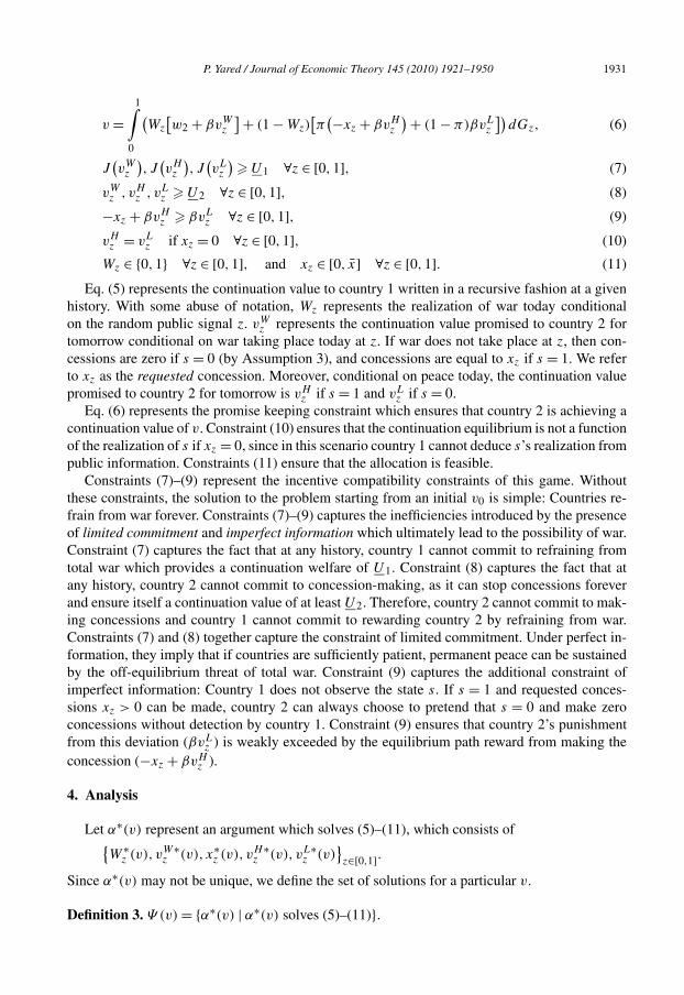
Eq. (5) represents the continuation value to country 1 written in a recursive fashion at a givenhistory. With some abuse of notation, Wz represents the realization of war today conditionalon the random public signal z. vW

z represents the continuation value promised to country 2 fortomorrow conditional on war taking place today at z. If war does not take place at z, then con-cessions are zero if s = 0 (by Assumption 3), and concessions are equal to xz if s = 1. We referto xz as the requested concession. Moreover, conditional on peace today, the continuation valuepromised to country 2 for tomorrow is vH

z if s = 1 and vLz if s = 0.

Eq. (6) represents the promise keeping constraint which ensures that country 2 is achieving acontinuation value of v. Constraint (10) ensures that the continuation equilibrium is not a functionof the realization of s if xz = 0, since in this scenario country 1 cannot deduce s’s realization frompublic information. Constraints (11) ensure that the allocation is feasible.

Constraints (7)–(9) represent the incentive compatibility constraints of this game. Withoutthese constraints, the solution to the problem starting from an initial v0 is simple: Countries re-frain from war forever. Constraints (7)–(9) captures the inefficiencies introduced by the presenceof limited commitment and imperfect information which ultimately lead to the possibility of war.Constraint (7) captures the fact that at any history, country 1 cannot commit to refraining fromtotal war which provides a continuation welfare of U1. Constraint (8) captures the fact that atany history, country 2 cannot commit to concession-making, as it can stop concessions foreverand ensure itself a continuation value of at least U2. Therefore, country 2 cannot commit to mak-ing concessions and country 1 cannot commit to rewarding country 2 by refraining from war.Constraints (7) and (8) together capture the constraint of limited commitment. Under perfect in-formation, they imply that if countries are sufficiently patient, permanent peace can be sustainedby the off-equilibrium threat of total war. Constraint (9) captures the additional constraint ofimperfect information: Country 1 does not observe the state s. If s = 1 and requested conces-sions xz > 0 can be made, country 2 can always choose to pretend that s = 0 and make zeroconcessions without detection by country 1. Constraint (9) ensures that country 2’s punishmentfrom this deviation (βvL

z ) is weakly exceeded by the equilibrium path reward from making theconcession (−xz + βvH

z ).

4. Analysis

Let α∗(v) represent an argument which solves (5)–(11), which consists of{W ∗

z (v), vW∗z (v), x∗

z (v), vH∗z (v), vL∗

z (v)}z∈[0,1].

Since α∗(v) may not be unique, we define the set of solutions for a particular v.

Definition 3. Ψ (v) = {α∗(v) | α∗(v) solves (5)–(11)}.


Let W ∗(v) = ∫ 10 W ∗

z (v) dGz and define vW∗(v) = ∫ 10 W ∗

z (v)vW∗z (v) dGz/W ∗(v). Define

x∗(v) = ∫ 10 (1 − W ∗

z (v))x∗z (v) dGz/(1 − W ∗(v)) and vH∗(v) and vL∗(v) analogously. Note that

given the concavity of (5) and the convexity of (6)–(11), a solution always exists in which theonly element of α∗(v) which depends on z is W ∗

z (v) so that{vW∗z (v), x∗

z (v), vH∗z (v), vL∗

z (v)} = {

vW∗(v), x∗(v), vH∗(v), vL∗(v)} ∀z.22 (12)

For the remainder of our discussion, we assume that countries are sufficiently patient thatpeace is incentive compatible for a positive mass of continuation values.23

Assumption 4. β > −w1/(πw2).

In the following three sections, we characterize important features of the solution to the recur-sive program in (5)–(11) (Section 4.1), and we use this characterization to describe the realizationof war and peace along the equilibrium path (Section 4.2) and in the long run (Section 4.3).

4.1. Characterization

In this section, we characterize the solution to (5)–(11) in the below proposition. We providea heuristic proof of this proposition in this section. Section 4.2 describes the economic intuitionfor this proposition together with its implications.

Proposition 2 (Characterization).

1. ∃U ∈ (U2,U2) s.t. ∀v � U and ∀α∗(v) ∈ Ψ (v), W ∗z (v) = 0 ∀z,

2. ∀α∗(v) ∈ Ψ (v) s.t. v � U

x∗(v) = min{βU2 − v, x}, vH∗(v) = min

{v + x

β,U2

}, and vL∗(v) = v/β,

(13)

and3. ∃α∗(v) ∈ Ψ (v) ∀v ∈ (U2, U ) s.t. W ∗(v) > 0 and vW∗(v) > U2.

The first part of this proposition states that above a continuation value U , war ceases to oc-cur. The second part of this proposition states that if v � U , the average requested concessionx∗(v) weakly decreases in v, and the average reward vH∗(v) and punishment vL∗(v) weakly risein v.24 More specifically, the exact characterization in (13) captures the fact that (i) either theaverage requested concession is maximal or the average reward is maximal (i.e., x∗(v) = x orvH∗(v) = U2) and (ii) (9) must bind. The last part of this proposition states that for continua-tion values v below U but above U2, there exist solutions for which war occurs and the averagecontinuation value following the realization of war exceeds U2.

This proposition is displayed graphically in Fig. 3. v is on the x-axis. On the y-axis, W ∗(v)

is in the in the top panel, x∗(v) is in the middle panel, and vH∗(v) and vL∗(v) are in the bottom

22 Note that some of these variables are undefined whenever they become irrelevant if either W∗(v) equals 0 or 1, butall of our results pertain to situations in which they are well defined.23 The precise implications of Assumption 4 are described in Appendix A.24 This is because v < 0 since v = 0 corresponds to permanent peace which is not incentive compatible.


Fig. 3. Recursive solution.

panel.25 Note that in some cases — particularly in the top panel which features W ∗(v) — thesedisplay correspondences. The left set of panels consider the case of a low cost of war to country 2(i.e., w2 > −x/β) and the right set of panels consider the case of a high cost of war to country 2(i.e., w2 < −x/β).26 Proposition 2 applies to both cases and we distinguish between the twocases in Section 4.3.

A heuristic proof of the first part of Proposition 2 is as follows. Countries can effectively ran-domize over the realization of war, and this ability to randomize implies a linearity in J (v) for thecontinuation values which are generated by the positive probability of war. Since W ∗(U2) = 1,it follows that there is an interval [U2, U ) over which the probability of war is positive and over

25 vW∗(v) is excluded due to space constraints.26 We do not display the knife-edge case with w2 = −x/β due to space constraints.


which J (v) is linear. This is displayed in Fig. 2. Thus, there exists a cutoff point U above whichwar ceases to occur since it reduces the welfare of both countries.27

A heuristic proof of the second part of Proposition 2 is as follows. To understand why it isnecessary that either x∗(v) = x or vH∗(v) = U2, consider a solution which satisfies (12) forv � U so that W ∗(v) = 0. Fix vL∗(v), and imagine if x∗(v) < x and vH∗(v) < U2. Then nec-essarily, a perturbation which increases x∗(v) by ε and vH∗(v) by ε/β for some ε > 0 which isarbitrarily small continues to satisfy (6)–(11). Moreover, the change in the welfare of country 1 isπ(ε + βJ (vH∗(v) + ε/β) − J (vH∗(v))) which is positive as long as the slope of J (·) is strictlyabove −1, which is the case in our framework. To see why, note that in an environment whichignores incentive compatibility constraints (7)–(9), the slope of J (·) would be −1. This is be-cause a transfer of 1 unit of welfare from country 1 to country 2 would occur through a reductionin concessions which the two countries equally value. In contrast, under (7)–(9), the transfer of1 unit of welfare from country 1 to country 2 occurs through a reduction in concessions as well asa reduction in the probability of future war, which is beneficial to both countries. Therefore, theimplied reduction in size of the concession is not as large so that the slope of J (·) exceeds −1.

An additional rationale for this result can be generated by imagining an environment whichignores the upper bound on xz in (11) as well as the lower bound on J (vH

z ) in (7). It can be shownthat in such a setting, the efficient solution always requires country 1 to reward country 2’s firstsuccessful concession with permanent peace. This is efficient since it allows country 1 to extractas much as possible in the current period while maximizing the duration of peace in the future,which is beneficial to both countries. This insight is related to the “generalized no distortion atthe top” result presented in Battaglini [8]. The result does not entirely hold in our environment(i.e. there may be a war even after a concession is made) because the upper bound on xz or thelower bound on J (vH

z ) will bind.28

To understand why it is that (9) must bind — which is also embedded in the second partof Proposition 2 — imagine if this were not the case, again considering a solution which sat-isfies (12). Then a perturbation which increases vL∗(v) by ε/β either by increasing x∗(v) byε(1 − π)/π or by reducing vH∗(v) by ε(1 − π)/(πβ) strictly raises welfare. This is becausean increase in vL∗(v) raises the welfare of country 1 by reducing the incidence of war goingforward. Technically, vH∗(v) and vL∗(v) are never inside the same line segment of J (v), so thatthe strict concavity of J (v) between these two points requires (9) to bind.

A heuristic proof of the third part of Proposition 2 is as follows. Consider a solution tothe program for v ∈ (U2, U ) for which W ∗(v) > 0 and vW∗(v) = U2 associated with someW ∗(v) < 1.29 Consider a perturbation which increases the probability of war W ∗(v) by ε andincreases the continuation value vW∗(v) by an amount (which is a function of ε) so as to leave(6) satisfied for some ε > 0 arbitrarily small. This continues to satisfy (6)–(11), and the linearityof J (·) in the interval [U2, U ] implies that this perturbation yields the same welfare to country 1as the original allocation. This idea is displayed in the top panel of Fig. 3 which shows that in theinterval (U2, U ), W ∗(v) is a correspondence. It can take on low values if vW∗(v) is chosen to

27 Note that by (8) and (9), U � βU2 > U2. Whether U equals or exceeds βU2 is important for characterization of thelong run in Section 4.3.28 More generally, in a situation in which country 1 can commit so that (7) can be ignored, U2 = 0 since country 1can credibly promise to never attack country 2. Much of our characterization would be preserved in this case withthe exception that one potential absorbing state in the long run is permanent peace following a sequence of successfulconcessions.29 If W∗(v) = 1, then v = U2 by definition.


be low, whereas it can take on high values if vW∗(v) is chosen to be high. Intuitively, country 1has flexibility in the intertemporal allocation of war. It can occur with high probability today, butwith lower probability in the future, or alternatively, it can occur with low probability today, butwith high probability in the future.

4.2. Equilibrium path

In this section, we use the results of Proposition 2 to characterize the dynamics of war andpeace along the equilibrium path. These are summarized in the below theorem where we letv = maxv{v ∈ [U2,U2] s.t. v = arg maxl J (l)}, the lowest continuation value on the downwardsloping portion of J (v), so that U2(α) � v0 in (4) always binds if v0 � v.30

Theorem 1 (Equilibrium path).

1. All solutions to (4) for all v0 feature Pr{Wt+k = 1|Wt = 0} > 0 ∀t for some k > 0, and2. There exists a solution to (4) for almost all v0 � v which features

Pr{Wt = 0 and Wt+k = 1 and Wt+l = 0} > 0

for some t � 0 and some l > k > 0.

The first part of Theorem 1 states that in the solution to (4), if peace occurs at some date t , thenwar must be expected with positive probability at some date t + k. In other words, the realizationof peace at any date must be followed by the positive probability of war in the future. The secondpart of Theorem 1 states that for almost all v0 � v, there exists a solution to (4) which admits asequence of allocations which feature temporary war with positive probability, where temporarywar is defined formally as the realization of peace followed by probabilistic war followed byprobabilistic peace.31

Both parts of this theorem are a direct implication of Proposition 2. To understand the proof ofthe first part of the theorem, note that if v > U , then W ∗(v) = 0 so that peace takes place today.Proposition 2 implies that for such v < U2,

vL∗(v) < v and vH∗(v) > v.32 (14)

Therefore, if a concession today is successful, the continuation value tomorrow increases, andby consequence, requested concessions tomorrow weakly decrease. Therefore, a reward for suc-cessful concessions is a reduction in future requested concessions. In contrast, if a concessiontoday is unsuccessful, the continuation value tomorrow decreases, and by consequence, any con-cession requested tomorrow must weakly increase. This incentive scheme enforces concessionsalong the equilibrium path, since country 2 will always make a concession when it is able to,since failure to do so can result in an increase in future requested concessions. Therefore, alongthe equilibrium path, a long sequence of failed concessions by country 2 can cause requestedconcessions by country 1 to incrementally increase, and by Theorem 1, war eventually becomes

30 We use W∗z (v) to refer to the probability of war in the recursive solution, whereas Wt = {0,1} corresponds to the

stochastic realization of war in period t .31 The theorem applies to almost all v0 � v because one can consider some environments where temporary wars do notoccur starting from a countable finite set of v0’s. See Appendix A for details.32 The fact that vH∗(v) > v is established in the proof of Proposition 2 since vH∗(U) � U+x � U .
β


necessary to enforce these ever-increasing concessions since continuation values decline beyondU with positive probability.

As an example, consider an environment in which x is arbitrarily large, so that the constraintthat xz � x never binds. In this scenario, Proposition 2 dictates that vH∗(v) = U2, x∗(U2) =(β − 1)U2, and vL∗(v) � U if v � U/β . Now imagine that along the equilibrium path country 1requests a concession xt from country 2, where associated with this concession is a continuationvalue vt � U/β promised to country 2. It follows from Proposition 2 that xt+1 = x∗(U2)+ xt/β

if the concession at t is unsuccessful and that xt+1 = x∗(U2) if it is successful.33 If vt+1 in theformer scenario exceeds U/β , then it follows that a subsequent failed concession at t + 1 causescountry 1 to request a concession xt+2 = x∗(U2) + xt+1/β at t + 2, and so on. Therefore, inthis simple example, country 1 always requests a base concession of size x∗(U2) plus accruedmissed concessions from the past, adjusting for discounting.

Why do failed concessions lead to escalating demands as opposed to immediate war? Thisis because war is costly to both countries, whereas larger concessions are only costly to coun-try 2 and beneficial to country 1. Therefore, a sequence of initial missed concessions does notlead automatically to war, but to escalating demands. Country 1 forgives country 2 for the firstmissed concessions by requesting larger and larger concessions.34 More specifically, it requestscompensation for previously missed concessions, to the extent allowed by the upper bound x.Country 1 would effectively like to postpone the realization of war as much as possible since itdestroys surplus and harms both countries. An important way in which country 1 can postponethe realization of war is by requesting high enough concessions from country 2 today so as toreward their success with as high a reward as possible. This works since a higher reward is as-sociated a longer duration of peace which benefits both countries going forward. Nevertheless,there is a limit to the feasibility of punishing country 2 with an increase in requested concessions,since beyond a certain point, requested concessions become so large that country 1 must punishtheir failure with the realization of war.

Efficient equilibria thus all begin on the downward sloping portion of J (·) in Fig. 2. Continua-tion values decline with positive probability if concessions fail until the two countries inevitablytransitions to the upward sloping portion of J (·). Once the two countries arrive at the upwardsloping portion of J (·), they recognize that it is necessary for them to engage in an inefficient in-teraction in order to sustain the efficient interaction which has taken place in the past. Moreover,countries realize that attempted cooperation has in fact occurred in the past: War is by no meansex-post necessary, though it is ex-ante required for the enforcement of peace.35

To understand the proof of the second part of Theorem 1, note that once continuation valueshave declined beyond U , Proposition 2 implies that war can take place with positive probabilitytoday and be followed by a continuation value which exceeds U2 starting from tomorrow. Sucha continuation value must necessarily assign a positive probability to peace going forward sincethe payoff to country 2 exceeds that of total war. The intuition for this result is as follows. Oneobvious and efficient method of punishing country 2’s failed concessions is for country 1 to en-gage in total war with low probability. What the theorem shows is that there exists an alternative

33 There is no randomization over the size of concessions in this example. The derivation of xt+1 follows from the factthat vt+1 = vt /β if st = 0, xt+1 = βU2 − vt+1, and xt = βU2 − vt .34 An equivalent version of our model in which concessions are binary features escalation in the form of an increasedprobability of requested concessions.35 More generally, efficient sequential equilibria here are not renegotiation proof. According to the definition of Farrelland Maskin [13], the only weakly renegotiation proof equilibrium in our setting is total war.


method of efficiently punishing country 2 which is to engage in a temporary war with high prob-ability. Both of these methods are equivalent from an efficiency perspective, and they deliver thesame continuation value to country 2. Consequently, conditional on the two countries arrivingto a history in the interval (U2, U ) — which is an event which occurs with positive probabilitystarting from almost all v0 � v — there is no need for country 1 to punish country 2’s failedconcessions with total war and temporary war can be generated along the equilibrium path.36

Theorem 1 delivers insights which build on the literature on repeated games. In particular,the first part of the theorem is related to the work of Green and Porter [20] who show that therealization of inefficient outcomes (such as price wars) can sustain efficient outcomes along theequilibrium path. In our setting, this insight implies that periods of peace are necessarily fol-lowed by periods of war. Without war, country 2 makes zero concessions, and by Assumption 2,country 1 cannot be satisfied by zero concessions. Note that as in Green and Porter [20], thisinsight applies here to all sequential equilibria, and not just efficient sequential equilibria.

The second part of the theorem also relates to the work of Green and Porter [20] since theseauthors present examples of sequential equilibria in which temporary price wars sustain coop-eration. Nonetheless, the realization of temporary wars in their examples do not necessarilycorrespond to the efficient sequential equilibria as they do in our framework. For this reason,our second result is more closely related to the work of Abreu, Pearce, and Stacchetti [2,3] whoanalyze the efficient solution to a set of games related to that of Green and Porter [20]. Theseauthors establish the necessity of the Bang–Bang property in the characterization of efficientequilibria. In this regard, our environment provides an example in which the satisfaction of theBang–Bang property is not necessary for efficiency. As a consequence, in our setting temporarywars can be featured in an efficient equilibrium, and they are generated by a path of continuationvalues which fail to satisfy the Bang–Bang property.

More specifically, in our context, the Bang–Bang property implies that continuation valuesonly travel to extreme points in the set of values Γ . Since all points on J (·) generated by prob-abilistic war are located on a line in the interval [U2, U ) (see Fig. 2), this implies that, if theBang–Bang property were necessary in our context, then any realization of war would need to beassociated with the absorbing state of total war. Thus, one would predict that in our framework,escalating demands and the failure to make concessions should necessarily lead directly to totalwar. What Theorem 1 shows is that even though such a dynamic path may be featured in anefficient equilibrium (i.e., satisfaction of the Bang–Bang property is sufficient for efficiency), analternate dynamic path with temporary wars may also be featured in an efficient equilibrium (i.e.,satisfaction of the Bang–Bang property is not necessary for efficiency).

The reason behind this is that information in our environment is coarse, and as a consequence,the Bang–Bang property — which is necessary in environments in which information is suffi-ciently rich — need not hold. More specifically, though country 1 is always certain that country 2is cooperating whenever concessions succeed, country 1 receives no information if concessionsfail, and it cannot deduce the likelihood that country 2 is genuinely unable to make a conces-sion. Therefore, there is a chance that country 1 is making a mistake by going to war. Thus,total war does not dominate temporary wars as a punishment device since there is a limit on theinformation which is available to country 1 when it decides on the extent of war.

36 Hauser and Hopenhayn [21] also present a game which features forgiveness, though their model considers the efficienttransfer of favors whereas ours concerns the use of the inefficient action of war in eliciting concessions.


This situation would be significantly different, for instance, if country 1 could observe a suf-ficient amount of information in periods in which concessions fail. For example, suppose thata continuous public signal y were revealed whenever concessions are zero, where this signaly is informative about the state s with higher values of y being more likely if s = 1 (i.e., thecost of concessions is low). In this situation, escalating demands would always be followed bythe stochastic realization of total war, with total war being more likely if concessions fail con-temporaneously with the realization of a sufficiently high signal y. Country 1 would effectivelyuse extreme rewards and punishments to provide incentives to country 2 while simultaneouslyutilizing the information in y to optimally reduce the probability of error in going to war.37 Ourmodel highlights why this mechanism fails to work once information becomes coarse. Country 1may make a mistake in going to total war, so that it does not strictly benefit from using such anextreme punishment.38

4.3. Long run

Our model generates temporary wars along the equilibrium path, and a natural questionconcerns the extent to which such temporary wars can be sustained in the long run. This isparticularly relevant for understanding conflicts which have lasted a significant length of timebut have not culminated in total war. We argue that even though temporary wars can occur alongthe equilibrium path, they can only be sustained in the long run if countries are sufficiently pa-tient (β is high), if the cost of war is sufficiently large (w2 is low), and if the cost of concessionsis sufficiently low (x is low).

Theorem 2 (Long run).

1. If w2 � −x/β , � a solution to (4) for any v0 s.t. limt→∞ Pr{Wt = 0} > 0,2. If w2 < −x/β , ∃ a solution to (4) for all v0 s.t. limt→∞ Pr{Wt = 0} = 0, and3. If w2 < −x/β , ∃ a solution to (4) for all v0 s.t. limt→∞ Pr{Wt = 0} > 0.

The first part of Theorem 2 states that if w2 � −x/β , meaning if the cost of war w2 is lowrelative to the discounted cost of the maximal concession −x/β , then there is no efficient se-quential equilibrium which features peace in the long run. Therefore, all allocations necessarilyconverge to total war. Together with Theorem 1, Theorem 2 effectively states that even thoughtemporary wars can occur along the equilibrium path, eventual convergence to total war is nec-essary. The second and third parts of Theorem 2 state that if instead w2 < −x/β , then thereexist efficient sequential equilibria which converge to total war as well as efficient sequentialequilibria which feature temporary war in the long run. Thus, though convergence to total warconstitutes an efficient equilibrium, convergence to total war is not necessary for efficiency. Notethat if w2 � −x/β , then the Bang–Bang property described in Section 4.2 necessarily holds in

37 Specifically, y has full support conditional on s and it satisfies the monotone likelihood ratio property. In this cir-cumstance, the failure of concessions cannot lead to continuation values in the interior of a line segment of J (v) for anypositive probability realizations of y since this would imply that country 1 is not exploiting the full informational contentof y. I thank Andrew Atkeson for pointing out this example.38 We conjecture that our result of temporary war holds for the intermediate case in which country 1 observes a signaly which has N realizations, with higher values being more likely if s = 1. As N → ∞, we should converge to thecontinuous signal case in which temporary war cannot occur with positive probability.


the long run, whereas if w2 < −x/β , the Bang–Bang property is not necessary even in the longrun.

A heuristic proof of the first part of Theorem 2 is as follows. One must first establish that inthis case, U = βU2, where U is the continuation value above which peace with probability 1strictly dominates probabilistic war and βU2 is the continuation value below which peace withprobability 1 ceases to be incentive compatible (since v/β � vL∗(v) � U2 by (9)). The reasonwhy peace strictly dominates war whenever it is incentive compatible is because concessions canbe rewarded with an increase in continuation value to country 2, and this reduces the incidenceof war in the future which benefits country 1 and maximizes efficiency. Formally, x is largeenough that one can choose vH∗(v) � v for all v which weakly exceed βU2. This means that anytemporary wars which take place in the interval (U2, U ) necessarily end at a breaking point inwhich country 2 receives promised utility U = βU2 conditional on peace. At this point, country 1gives country 2 a second chance at peace and requests a concession. If this concession fails, thentotal war ensues since vL∗(U) = U2. Alternatively, if this concession succeeds, country 2 isrewarded and peace ensues. Nonetheless, by Theorem 1 such a peace leads to a future war withpositive probability which can involve either a total war or a temporary war which again ends atthe breaking point. Because concessions can always fail with positive probability at the breakingpoint, and because the failure of concessions at the breaking point lead to total war, total war inthis case is unavoidable in the long run.39

A heuristic proof of the second and third parts of Theorem 2 is as follows. Because the satis-faction of the Bang–Bang property is sufficient for efficiency, one can easily construct examplesin which the first realization of war — which is necessary by Theorem 1 — is associated withtotal war, which explains the second part of the theorem. To understand the third part of thetheorem, note that in this case U > βU2, so that even if peace with probability 1 is incentivecompatible, it need not be strictly optimal. Specifically if v is between βU2 and U , then peacewith probability 1 and probabilistic war are equally efficient means of providing continuationvalue v to country 2. This is because in this region, x∗(v) = x and vH∗(v) � U , so that even ifpeace takes place today and if concessions are successful today, war cannot be avoided in thefuture since otherwise country 2 would not be receiving the same continuation value. In otherwords, concessions today cannot be made large enough so as to allow country 1 to forgive coun-try 2 for past failed concessions going forward. More generally, the failure of concessions alongthe equilibrium path leads continuation values to eventually decline beyond U and to effectivelycross a war barrier from which there is no return to higher continuation value. Because peacewith probability 1 in this region can be associated with a continuation value which exceeds βU2,the failure of concessions need not be punished with total war since one can always choosevL∗(v) > U2.40 Thus, total war is not required for the enforcement of incentives and temporarywars can occur forever.

The intuition for the first part of the theorem is as follows. If w2 is high and β is low, thenthe cost of total war to country 2 is low relative to the cost of the maximal concession of size x.As a consequence, it is necessary for country 1 to use the most extreme punishment to induceconcessions from country 2, since the weaker punishment of temporary war cannot induce theselarge concessions. More specifically, since assured peace takes place whenever it is incentive

39 In other words, a transition path which avoids total war occurs with probability zero since concessions would need tosucceed every single time the breaking point is reached.40 These facts are displayed in Fig. 3b which shows that the probability of war and continuation values as a function ofv are correspondences for continuation values below U .


compatible (i.e., U = βU2), the duration of peace is prolonged as much as possible along theequilibrium path. Nonetheless, this comes at a cost in the long run since eventually, a long streamof concessions fail, and this leads to inevitable total war.41 Therefore, the two countries sacrificetheir welfare in the long run in exchange for efficient incentive provision along the equilibriumpath. Note that if w2 � −x, convergence to total war takes place even as β approaches 1.42

The intuition for the second and third parts of the theorem are as follows. If w2 < −x/β ,then the cost of total war to country 2 is extremely high relative to the cost of the maximalconcession of size x. As a consequence, though country 1 could use the most extreme punishmentto induce concessions from country 2, this is not necessary for efficiency. This is because theweaker punishment of temporary wars is sufficiently painful. Specifically, peace with probability1 does not strictly dominate probabilistic war in the range (U2, U ) since successful concessionscannot be rewarded with the prolongation of the peace. Therefore, there is no sense in whichthe two countries maximize the duration of peace along the equilibrium path at the cost of totalwar in the long run. Specifically, even if a very long sequence of concessions fails in the longrun, countries do not converge to total war because every missed concession can be punishedwith a war which stochastically ends with another chance at peace and this provides sufficientinducement for concessions.

Note that an implication of our model is that an increase in x from below −βw2 toabove −βw2 leads countries away from the possibility of long run temporary wars to thenecessity of long run total war. An important point to bear in mind is that this trans-formation increases period 0 welfare. The reason is that if x increases, it becomes eas-ier for the two countries to postpone the realization of war, since escalating demands asopposed to war can be more easily used by country 1 to provide inducements to coun-try 2. Rather than fight at a particular date, country 1 can request even larger concessionsfrom country 2 and leave war for a later date. This raises welfare along the equilibriumpath by prolonging the duration of peace. Nevertheless, this is made at the cost of totalwar in the long run which becomes necessary to induce the increase in concessions underpeace.

To understand the role of the upper bound x in generating these distinct long run outcomes inour environment, it is useful to consider a more general environment in which the upper bound onconcessions x is ignored but where country 2 experiences a cost of concessions equal to −e(xt )

if st = 1 for some increasing function e(·). One can show that in this modified environment, warscontinue to occur with positive probability only if v ∈ [U2, U ). Moreover, by analogous reason-ing to our previous arguments, convergence to total war is necessary in the efficient sequentialequilibrium if U = βU2, though it is not necessary if U > βU2. Importantly, it can be shownthat if e(·) is a continuous function, then necessarily U = βU2 so that convergence to total war isnecessary for efficiency. This is because starting from an equilibrium in which country 2 receivesβU2 via peace with probability 1, country 1 optimally requests a high enough concession so asto choose an incentive compatible reward vH∗(βU2) � βU2 since this benefits country 1 sinceit reduces the incidence of war going forward. In contrast, it may no longer be true that peace

41 Note that if in every period there is a positive probability that the government in country 1 is replaced by a governmentwhich does not remember the past, then the equilibrium restarts from some initial v0 following such a shock. One canshow that total war would be avoided in this case, though efficiency would be reduced since this undermines the disciplineon country 2. Details available upon request.42 It is nevertheless the case that the probability of total war also approaches zero since vL∗(v) approaches v and thedecrease in continuation value approaches zero (see Proposition 2).


with probability 1 strictly dominates probabilistic war at v = βU2 if instead e(·) is a discontinu-ous function. This is because starting from an equilibrium in which country 2 receives βU2 viapeace with probability 1, vH∗(βU2) < βU2 and a perturbation which increases concessions atv = βU2 requires an increase in vH which is either too high to be incentive compatible or toohigh to be efficient from the perspective of country 1 since it reduces concessions by too muchgoing forward.43 Therefore, if e(·) is discontinuous at particular values of xt , it may be the casethat U > βU2 so that temporary wars can be featured in the efficient equilibrium. In sum, ourenvironment considers a special case of this more general environment in which e(xt ) = xt forxt ∈ [0, x] and e(xt ) is arbitrarily large for xt > x. Thus, the exact value of x — which corre-sponds to the maximal cost of concessions in equilibrium — determines whether U exceeds oris equal to βU2.

5. Conclusion

We have analyzed a dynamic model of war and peace to determine whether and how tem-porary wars between two countries can occur. In doing so, we have characterized the dynamicsof escalation and highlighted how imperfect information generates temporary wars. Moreover,we present conditions which are necessary for the two countries to avoid total war and engagein temporary wars in the long run. Our analysis shows that countries which escalate to total warreach a breaking point at the culmination of every temporary war. In contrast, countries which areable to avoid total war find themselves having passed a war barrier beyond which forgiveness inthe form of lower demands by the aggressive country become impossible. Our analysis providesus with a framework for understanding which conflicts can be sustained without convergence tototal war.

There are some important caveats in interpreting our results. First, we have ignored the factthat the cost of concession can be persistent by assuming that the state is i.i.d. This assump-tion is not made for realism but for convenience since it maintains the common knowledgeof preferences over continuation contracts and simplifies the recursive structure of the effi-cient sequential equilibria. Future work should consider the effect of relaxing this assumptionand potentially using some of the tools in Fernandes and Phelan [16] in this regard. Sec-ond, we have ignored the possibility that the aggressive country may be able to exert someeffort in more effectively monitoring its rival. In such an environment, both the precisionas well as the coarseness of public signals becomes endogenous, and given our discussionin Section 4.2, this will affect the extent to which war is necessary as well as the extentto which temporary war can be sustained in an efficient equilibrium. Third, in choosing tofocus on the role of diplomatic concessions, we have ignored the fact that military conces-sions such as disarmament could also serve to avert conflict by altering the payoff from war.Finally, we have implicitly assumed that there is a single good over which the two coun-tries bargain and that in every period concessions are one sided. A realistic extension of thisframework is one in which bilateral concessions are necessary to sustain peace. In such asetting, both countries could potentially have an incentive to engage in war. A thorough in-vestigation of the implications of these issues for our results would be interesting for futureresearch.

43 Such a perturbation unambiguously benefits country 1 if vH is rising on the upward sloping portion of J (·) but itdoes not unambiguously do so if vH is on the downward sloping portion. Details available upon request.


Appendix A

A.1. Proofs for Section 3

A.1.1. Proof of Proposition 1Step 1. If α is a sequential equilibrium allocation, then xt (qt , zt , st = 0) = 0 ∀(qt , zt ) whereWt(qt , zt ) = 0. If instead xt (qt , zt , st = 0) > 0, consider a deviation by country 2 at (qt , zt , st =0) to x′

k(qk, zk, sk) = 0 ∀k � t and ∀(qk, zk, sk) which yields a minimum continuation value ofβU2. Since xt (qt , zt , st = 0) is bounded from below by 0 so that E{U2(α|qt+1,zt+1) | qt , zt , st } isbounded from above by 0, if this deviation is weakly dominated, then it must be that −c � βU2,but this violates Assumption 3.

Step 2. The necessity of (2) for i = 1 follows from the fact that country 1 can chooseW ′

k(qk, zk) = 1 ∀k � t and ∀(qk, zk) and this delivers continuation value U1. The necessityof (2) for i = 2 follows from the fact that country 2 can choose x′

k(qk, zk, sk) = 0 ∀k � t and∀(qk, zk, sk), and this delivers a minimum continuation value U2. The necessity of (3) fol-lows from the fact that conditional on Wt(qt , zt ) = 0, country 2 can unobservably deviate tox′t (qt , zt , st = 1) = xt (qt , zt , st = 0) = 0 and follow the equilibrium strategy associated with

(qt , zt , st = 0) thereafter.

Step 3. For sufficiency, consider an allocation in which xt (qt , zt , st = 0) = 0 ∀(qt , zt ) whichalso satisfies (2) and (3), and construct the following off-equilibrium strategy. Any observabledeviation results in a reversion to the repeated static Nash equilibrium. We only consider sin-gle period deviations since β < 1 so that continuation values are bounded. If Wt(qt , zt ) = 1,a deviation to W ′

t (qt , zt ) = 0 is strictly dominated by (2) since βU1 < U1. If Wt(qt , zt ) = 0, a de-viation to W ′

t (qt , zt ) = 1 is weakly dominated by (2). If Wt(qt , zt ) = 0, any deviation to x′t (qt , zt ,

st = 1) > 0 is weakly dominated by a deviation to x′t (qt , zt , st = 1) = xt (qt , zt , st = 0) = 0 since

E{U2(α|qt+1,zt+1) | qt , zt , st = 0} � U2. A deviation to x′t (qt , zt , st = 1) = 0 is weakly domi-

nated by (3). Any deviation to x′t (qt , zt , st = 0) �= xt (qt , zt , st = 1) is strictly dominated since

c > 0. Since E{U2(α|qt+1,zt+1) | qt , zt , st = 1} � 0, by Assumption 3 and (2), a deviation tox′t (qt , zt , st = 0) = xt (qt , zt , st = 1) is strictly dominated.

A.1.2. Proof of Lemma 1Step 1. Consider two continuation value pair {U ′

1,U′2} ∈ Γ and {U ′′

1 ,U ′′2 } ∈ Γ with correspond-

ing allocations α′ and α′′. It must be that{Uκ

1 ,Uκ2

} = {κU ′

1 + (1 − κ)U ′′1 , κU ′

2 + (1 − κ)U ′′2

} ∈ Γ ∀κ ∈ (0,1).

Define ακ = {ακ |q0,z0}z0∈[0,1] as follows:

ακ |q0,z0 ={

α′|q0,

z0κ

if z0 ∈ [0, κ),

α′′|q0,

z0−κ

1−κ

if z0 ∈ [κ,1],where α′|

q0,z0κ

for z0 ∈ [0, κ) is identical to α′|q0,z0 with the exception that z0κ

replaces z0 in all

information sets qt , and α′′|q0,

z0−κ

1−κ

for z0 ∈ [κ,1] is analogously defined. ακ achieves {Uκ1 ,Uκ

2 },and since α′, α′′ ∈ Λ, then ακ ∈ Λ.

Step 2. Γ is bounded since Ui(α) is bounded for i = 1,2.


Step 3. To show that Γ is closed, consider a sequence {U ′1j ,U

′2j } ∈ Γ such that

limj→∞{U ′1j ,U

′2j } = {U ′

1,U′2}. There exists one corresponding sequence of allocations α′

j

which converges to α′∞ since Ui(α′j ) is continuous in α′

j . Since every element of α′j at (qt , zt )

is contained in {0,1} × [0, x]2, and since (2) and (3) are weak inequalities, then Λ is closedand α′∞ ∈ Λ. Since β ∈ (0,1), then by the Dominated Convergence Theorem, Ui(α

′∞) = U ′i for

i = 1,2. Therefore {U ′1,U

′2} ∈ Γ so that Γ is compact.

Step 4. To show that J (U2) = J (U2) = U1, note that it is not possible that J (·) < U1 since thisviolates (2) for i = 1.

Step 5. Imagine if J (U2) > U1 and consider the associated α. By Assumptions 1 and 2and Eq. (2) for i = 2, Eq. (3) implies that U2(α|q0,z0) � βU2 > U2 if W0(q0, z0) = 0.Since U2(α|q0,z0) � U2, then U2(α|q0,z0) = U2 and W0(q0, z0) = 1 ∀(q0, z0). This requiresE{U2(α|q1,z1) | q0, z0} = U2 ∀(q0, z0) and therefore U2(α|q1,z1) = U2 ∀(q1, z1). Forward in-duction on this argument implies that Wt(qt , zt ) = 1 ∀(qt , zt ) so that J (U2) = U1.

Step 6. Imagine if J (U2) > U1 and consider the associated α. Since U2(α|q0,z0) � U2, thenU2(α|q0,z0) = U2 ∀(q0, z0) in order that U2(α) = U2. If W0(q0, z0) = 1, then U2 = w2 +βE{U2(α|q1,z1) | q0, z0} � w2 + βU2, which means that U2 = U2 and by step 5, J (U2) = U1.Now consider W0(q0, z0) = 0. It must be that x0(q0, z0) = 0 and E{U2(α|q1,z1) | q0, z0} = U2,otherwise it is possible to reduce x0(q0, z0) or increase E{U2(α|q1,z1) | q0, z0} while maintaining(2) and (3) and strictly increasing U2(α|q0,z0). This means that U2 = βU2, but this violates thefact that U2 < 0, since U2 = 0 is not incentive compatible. This is because by Assumption 1,J (U2) + U2 � 0, so that if U2 = 0, then J (U2) � 0, which violates (2) for i = 1.

Step 7. It follows that J (v) is weakly concave since J (U2) = J (U2) = U1, J (v) � U1 ∀v ∈[U2,U2] by (2), and Γ is a convex set.

A.1.3. Implications of Assumption 4Assumption 4 implies that J (v) > U1 for some v. To see why, construct the following

equilibrium. If st−1 = 1, then Wt = 0 and xt = x = w1/π + ε if st = 1 and xt = 0 other-wise for ε > 0 arbitrarily small so as to continue to satisfy −w1 − πε > w2. If st−1 = 0,both countries revert to the repeated static Nash equilibrium forever. Let W0 = 0. By Assump-tion 1, country 1’s welfare strictly exceeds U1 and country 2’s welfare weakly exceeds U2so that (2) is satisfied. To check (3), let U2|s=1 represent the continuation value to country 2conditional on successful concessions yesterday. The stationarity of the equilibrium impliesU2|s=1 = −πx + β(πU2|s=1 + (1 − π)U2), so that (3) which requires −x + βU2|s=1 � βU2becomes −x � βw2 which is guaranteed by Assumption 4.

A.2. Proofs for Section 4

A.2.1. Proof of Proposition 2We prove each part of this proposition separately as well as additional needed results. We use

the following simplifying notation throughout:

Υ +(v, ε) = J (v + ε) − J (v)and Υ −(v, ε) = J (v) − J (v − ε)

.
ε ε


Proof of Part 1.Step 1. Consider two continuation values U ′ < U ′′ s.t. W ∗(U ′) > 0 and W ∗(U ′′) > 0. It followsthat

J (v) = J(U ′) + m

(v − U ′) ∀v ∈ [

U ′,U ′′] where m = J (U ′′) − J (U ′)U ′′ − U ′ . (15)

To see why, let

vF∗(v) = w2 + βvW∗(v), (16)

vP∗(v) = π(−x∗(v) + βvH∗(v)

) + (1 − π)βvL∗(v). (17)

For a given v with an associated solution α∗(v), one can choose a perturbation of this solutionwhich satisfies (12). Since this perturbation also satisfies (6)–(11), optimality and the concavityof J (·) imply

J (v) = W ∗(v)J(vF∗(v)

) + (1 − W ∗(v)

)J(vP∗(v)

). (18)

By (18) and the concavity of J (·), it follows that vF∗(v) and vP∗(v) are on the same line segment

in J (·) for a given v. Moreover, since vW∗(vF∗(v)) = vF∗(v)−w2β

> vF∗(v), it follows that

J (vF∗(U ′′)) − J (vF∗(U ′))vF∗(U ′′) − vF∗(U ′)

=(J(

vF∗(U ′′)−w2β

) − J(

vF∗(U ′)−w2β

))vF∗(U ′′)−vF∗(U ′)

β

,

where we have used the fact that J (vF∗(v)) = w1 +βJ (vW∗(vF∗(v))). By the concavity of J (·),vF∗(U ′) and vF∗(U ′′) are on the same line segment, and by the previous argument, they are onthe same line segment as vP∗(U ′) and vP∗(U ′′). Therefore, U ′ and U ′′ are on the same linesegment and (15) applies.

Step 2. Since W ∗(U2) = 1 by step 5 of the proof of Lemma 1, it follows from step 1 that(15) applies for U ′ = U2 and some U ′′ = U � U2. Imagine if U = U2. Then W ∗(v) = 0 forv = U2 + ε ∀ε > 0 arbitrarily small. By (9), this implies that v � βvL∗(v) � βU2 > U2 whichcannot be true for ε < −w2, leading to a contradiction. Therefore, U > U2.

Step 3. By Lemma 1 and Assumption 4, m > 0 and U < U2 so that

Υ +(U , ε) < m and Υ −(U , ε) = m. � (19)

Proof of additional lemmas

Lemma 2. The following properties hold:

1. If w2 � −x/β , then U = βU2, and2. If w2 < −x/β then U > βU2.

Proof.Step 1. Imagine if U < βU2. This violates (8) and (9) which require U � βvL∗(U) � βU2.

Step 2. J (v + ε) > J (v) − ε for ε > 0. If instead ∃v s.t. Υ −(v, ε) � −1, then by Lemma 1 andpart 1, ∃U ∈ [U ,U2) s.t. Υ +(U , ε) � −1 and Υ −(U , ε) > −1, so that W ∗(U) = 0. Consider


α∗(U) ∈ Ψ (U) which satisfies (12) and under which (9) binds, which is always weakly optimalby the weak concavity of the program and convexity of the constraint set. If x∗(U) > 0, thenoptimality requires that

J (U + ε) � π(x∗(U) − ε + βJ

(vH∗(U)

)) + (1 − π)βJ

(vL∗(U ) + ε

β

)(20)

since a perturbation to x′(U + ε) = x∗(U) − ε, vH ′(U + ε) = vH∗(U), and vL′(U + ε) =vL∗(U) + ε

βsatisfies (6)–(11) for v = U + ε. Subtraction of J (U) from both sides of (20)

yields Υ +(U , ε) � −π + (1 − π)Υ +( Uβ

, εβ) > −1, which is a contradiction where we have

used the fact that vβ

< v < 0 from step 6 of the proof of Lemma 1. If instead x∗(U) = 0 so

that vH∗(U) = vL∗(U) = Uβ

, then analogous arguments can be made with a perturbation to

x′(U +ε) = x∗(U) and vH ′(U +ε) = vL′(U +ε) = vβ

+ εβ

, so that Υ +(U , ε) � Υ +( Uβ

, εβ) > −1

which is also a contradiction.

Step 3. ∀v ∈ [U2,U2] and ∀α∗(v) ∈ Ψ (v), if W ∗z (v) = 0 then x∗

z (v) = x or vH∗z (v) = U2 ∀z.

If x∗(v) < x and vH∗(v) < U2, then consider a perturbation to x′z(v) = x∗(v) + ε, vH ′

z (v) =vH∗(v) + ε/β , and vL′

z (v) = vL∗(v) ∀z. Such a perturbation satisfies (6)–(11) and strictly im-proves welfare by step 2.

Step 4. Consider if w2 � −x/β and imagine if U > βU2. Let JP (v) denote the value of theconstrained program (5)–(11) s.t. W ∗(v) = 0. By the proof of part 1, JP (v) � J (v) for v < U

and JP (v) = J (v) for v � U . Therefore,

m = Υ −(U , ε) � JP (U) − JP (U − ε)

ε(21)

for ε > 0 arbitrarily small. By step 3, x∗(v) = x or vH∗(v) = U2, and by the same rea-

soning as step 2, (9) can bind. Therefore, if U+xβ

> U2, then JP (U)−JP (U−ε)ε

= −π +(1 − π)Υ −( U

β, ε

β) < m, but this contradicts (21). If U+x

β� U2, then JP (U)−JP (U−ε)

ε=

πΥ −( U+xβ

, εβ) + (1 − π)Υ −( U

β, ε

β) < m, but this also contradicts (21). This establishes the

first part of the lemma.

Step 5. Consider if w2 < −x/β and imagine if U = βU2. This implies that (19) holds for U =βU2. By part 1, W ∗(βU2) = W ∗(βU2 + ε) = 0 for ε > 0 arbitrarily small. By step 3, x∗(v) = x

or vH∗(v) = U2 and (9) may bind for v = βU2 and v = βU2 +ε by the same reasoning as step 2.

Since U+xβ

< βU2 � U2, then Υ +(U , ε) = πΥ +( U+xβ

, εβ) + (1 − π)Υ +( U

β, ε

β) = m, but this

contradicts (19). �Lemma 3. If α∗(v) ∈ Ψ (v) then it satisfies (6)–(11),

1. W ∗z (v) = 0 ∀z if v � U ,

2. vW∗z (v) � U ∀z,

3. π(−x∗z (v) + βvH∗

z (v)) + (1 − π)βvL∗z (v) � U ∀z if v � U ,

4. x∗z (v) = x or vH∗

z (v) = U2 ∀z, and5. (9) binds ∀z if v � U .


Proof.Step 1. The necessity of (6)–(11) follows by definition. The necessity of W ∗

z (v) = 0 ∀z if v � U

follows from part 1. The necessity of x∗z (v) = x or vH∗

z (v) = U2 ∀z follows from step 3 of theproof of Lemma 2.

Step 2. Imagine if vW∗z (v) > U for some z. Perturb the allocation as in step 1 of the proof of

part 1. By step 1 of the proof of part 1, Υ −(vW∗(v), ε) = m so that vW∗(v) � U by the concavityof J (·). Therefore, in order that this perturbation not strictly improve welfare, it is necessary thatΥ +(vW∗

z (v), ε) = m ∀z, which by (19) implies a contradiction.

Step 3. Imagine if π(−x∗z (v) + βvH∗

z (v)) + (1 − π)βvL∗z (v) > U for v � U . Perturb the alloca-

tion as in step 1 of the proof of part 1. By step 1 of the proof of part 1, Υ −(vP∗(v), ε) = m andwhich by the concavity of J (·) implies vP∗(v) � U . In order that this perturbation not strictlyimprove welfare, it is necessary that

Υ +(π

(−x∗z (v) + βvH∗

z (v)) + (1 − π)βvL∗

z (v), ε) = m ∀z,

which by (19) implies a contradiction.

Step 4. Imagine if (9) does not bind for some z if v � U . If x∗(v) < x, consider a perturbationto x′

z(v) = x∗(v), vH ′z (v) = v+x∗(v)

β< vH∗(v), and vL′

z (v) = vβ

> vL∗(v) ∀z. Such a perturbationsatisfies (6)–(11) and weakly increases welfare by the concavity of J (·). However, the perturbedallocation is suboptimal by step 3 of the proof of Lemma 2 since x′

z(v) < x and vH ′z (v) < U2.

Step 5. If instead x∗(v) = x, denote v = U ′. If the perturbation of step 4 does not strictly improvewelfare, then

Υ +(v, ε) = Υ +(

v + x

β, ε

)= Υ +

(v

β, ε

)(22)

for ε > 0 arbitrarily low and v = U ′. Note that since, Υ +(v, ε) = m for v < U , it must be given(19) that U ′ � βU > U so that Υ +(U ′, ε) < m. By step 1 of the proof of part 1 and steps 2and 3 of the proof of Lemma 2, ∀v ∈ [U ,U ′], there exists a solution to (5)–(11) s.t. x∗

z (v) = x

for which (9) binds so that vH∗z (v) = v+x

βand vL∗

z (v) = vβ

∀z. Therefore, ∀v ∈ [U ,U ′],

Υ +(v, ε) = πΥ +(

v + x

β,ε

β

)+ (1 − π)Υ +

(v

β,ε

β

), (23)

which by the concavity of J (·), the fact that Υ +( Uβ

, ε) = m, and (22) implies that

Υ +(U ′, ε) = m, leading to a contradiction. �Proof of Part 2.Step 1. Consider α∗(v) ∈ Ψ (v) for v � U . Define

vz = π(−x∗

z (v) + βvH∗z (v)

) + (1 − π)βvL∗z (v),

where by (6) and part 1, v = ∫ 10 vz dGz.


Step 2. By steps 4 and 5 of the proof of Lemma 3, it is necessary that for a given v � U

x∗z = min{βU2 − vz, x}, vH∗

z = min

{vz + x

β,U2

}, and vL∗

z = vz/β. (24)

Step 3. Optimality and the concavity of J (·) requires that J (v) = ∫ 10 J (vz) dGz so that all vz’s lie

on the same line. Note that x∗z = βU2 − vz (= x) and vH∗

z = U2 (= vz+xβ

) ∀vz � (�)βU2 − x.We can show that

Υ +(βU2 − x, ε) < Υ −(βU2 − x, ε), (25)

which means that two values of vz cannot be on different sides of βU2 − x. This follows fromthe fact that

Υ +(βU2 − x, ε) = −π + (1 − π)Υ +(

βU2 − x

β,ε

β

),

Υ −(βU2 − x, ε) = πΥ −(

U2,ε

β

)+ (1 − π)Υ −

(βU2 − x

β,ε

β

),

where (25) follows from step 2 of the proof of Lemma 2 and the concavity of J (·). Therefore,either vz � βU2 − x ∀z or vz � βU2 − x ∀z.

Step 4. Integrating every term in (24) over z yields (13).

Proof of additional corollary

Corollary 1. If an allocation α(v) satisfies Lemma 3’s conditions and (12), then α(v) ∈ Ψ (v).

Proof.Step 1. Let v � U and consider a hypothetical allocation α(v) which satisfies the conditions.Imagine if α(v) /∈ Ψ (v). Now consider the actual solution α∗(v) ∈ Ψ (v), perturb the solution asin step 1 of the proof of part 1 so that it satisfies (12). This implies that α∗(v) = α(v) /∈ Ψ (v),leading to a contradiction.

Step 2. If v < U , consider the case with w2 � −x/β . Satisfaction of the conditions entailsvF (v) = w2 +βvW(v) ∈ [U2,w2 +βU ] and vP (v) = βU2 = U for vF (v) and vP (v) defined in(16) and (17) under the proposed allocation. Suboptimality would imply that

J (v) > W(v)(w1 + βJ

(vW (v)

)) + (1 − W(v)

)J (U), (26)

for W(v) = U−v

U−vF (v), but (26) contradicts (15).

Step 3. If v < U , consider the case with w2 < −x/β . Satisfaction of the conditions entailsvF (v) = w2 + βvW(v) ∈ [U2,w2 + βU ] and vP (v) ∈ [βU2, U ]. Suboptimality and (15) wouldimply that

J (v) > W(v)(w1 + βJ

(vW (v)

))+ (

1 − W(v))(

πx + β

(U1 + m

(vP (v) + πx − U2

))), (27)

β


for W(v) = vP (v)−v

vP (v)−vF (v)if vF (v) � v � vP (v) and W(v) = vF (v)−v

vF (v)−vP (v)if vF (v) � v � vP (v).

However, (15) together with the fact that W(U) = 0 imply that

U1 + m(U − U2) = πx + β

(U1 + m

(U + πx

β− U2

)),

so that (27) contradicts (15). �Proof of Part 3. By Lemma 3 and Corollary 1, ∃α∗(v) ∈ Ψ (v) s.t. W ∗(v) � 0 and vW∗(v) > U2∀v ∈ (U2, U ). �A.2.2. Proof of Theorem 1

Proof of Part 1. Imagine if Pr{Wt+k = 1 | Wt = 0} = 0 ∀t and ∀k > 0. Constraint (9) impliesthat Pr{vt+1 � vt/β < vt | Wt = 0} = 1 − π , so that Pr{vt+k ∈ [U2, βU2)} > 0 for all t and forsome k > 0. However, it cannot be the case that Pr{Wt+k = 1 | vt+k ∈ [U2, βU2)} = 0 since from(8) and (9), this would require that vt+k � βU2 which is a contradiction.

Proof of Part 2. Since Pr{Wt+k = 1 | Wt = 0} > 0 by part 1, and since W0 = 0 since continua-tion values begin above v which weakly exceeds U , the absence of temporary wars implies thatPr{Wt+k = 0 | Wt = 1} = 0 ∀t � 0 and ∀k > 0. Construct a solution using Corollary 1 startingfrom some v0 ∈ [v,U2] s.t. v0 /∈ βT U2 for some integer T . Since (9) binds for v � U , thenPr{vt+1 = v/β < v | vt = v} = 1 − π > 0. Therefore, ∃t s.t. Pr{vt ∈ (U2, U )} > 0 and by Corol-lary 1, there exists a solution at vt ∈ (U2, U ) s.t. Pr{Wt = 1 | vt ∈ (U2, U )} > 0 and Pr{Wt+1 =0 | Wt = 1, vt ∈ (U2, U )} > 0 since Pr{vt+1 ∈ (U2, U ) | Wt = 1, vt ∈ (U2, U )} > 0. �A.2.3. Proof of Theorem 2

Proof of Part 1.Step 1. If w2 � −x/β , imagine if ∃ a solution to (4) s.t. limt→∞ Pr{Wt = 0} > 0, and consider apotential long run distribution of v. Since Pr{vt+1 = U2 | vt = U2} = 1, by step 5 of the proof ofLemma 1, then Pr{vt = U2} = 0 under this long run distribution.

Step 2. If v ∈ (U2, βU2), then from Lemma 3, vW∗z (v) � βU2 ∀z and vL∗

z (v) = U2 ∀z. There-fore,

Pr{vt+1 = U2

∣∣ Wt = 0, vt ∈ (U2, βU2)} = 1 − π, and (28)

Pr{vt+1 � βU2

∣∣ Wt = 1, vt ∈ (U2, βU2)} = 1 (29)

under the long run distribution of v.

Step 3. From (28),

Pr{vt+1 = U2} � Pr{vt ∈ (U2, βU2)

} × Pr{Wt = 0 | vt ∈ (U2, βU2)

} × (1 − π)

under the long run distribution. In order that Pr{vt+1 = U2} = 0, it is necessary that Pr{Wt =0 | vt ∈ (U2, βU2)} = 0. This is because Pr{vt ∈ (U2, βU2)} > 0 since Pr{vt = U2} = 0 andsince part 1 of Proposition 2 and part 1 of Theorem 1 imply that Pr{vt ∈ [U2, βU2)} = Pr{vt =U2} + Pr{vt ∈ (U2, βU2)} > 0.


Step 4. The fact that Pr{Wt = 1 | vt ∈ (U2, βU2)} = 1 combined with (29) implies Pr{vt+1 ∈(U2, βU2) | vt ∈ (U2, βU2)} = 1, and by forward induction

Pr{Wk = 1 ∀k � t + 1

∣∣ vt ∈ (U2, βU2)} = 1.

Since Pr{vt ∈ (U2, βU2)} > 0, then Pr{Wk = 1 ∀k � t + 1} = Pr{vt+1 = U2} > 0 which is acontradiction.

Proof of Part 2.Step 1. If w2 < −x/β , by Corollary 1, ∀v ∈ (U2, U ), ∃α∗(v) ∈ Ψ (v) s.t. W ∗(v) = U−v

U−U2,

vW∗z (v) = U2, x∗

z (v) = x, vH∗z (v) = U+x

β, and vL∗

z (v) = Uβ

∀z.

Step 2. Construct an equilibrium with the property of step 1, and imagine if limt→∞ Pr{Wt =0} > 0. Then it must be that Pr{vt = U2} = 0 under the long run distribution. However, in such an

equilibrium, Pr{vt+1 = U2 | vt ∈ (U2, U )} = U−vt

U−U2> 0 under the long run distribution. By part 1

of Proposition 2 and part 1 of Theorem 1 , Pr{vt ∈ [U2, U )} > 0. Consequently, Pr{vt = U2} > 0under the long run distribution.

Proof of Part 3.Step 1. If w2 < −x/β , by Corollary 1, ∀v ∈ (U2, U ), ∃α∗(v) ∈ Ψ (v) s.t. W ∗(v) = U−v

U−(U2+ε(v)),

vW∗z (v) = U2 + ε(v)

β, x∗

z (v) = x, vH∗z (v) = U+x

β, and vL∗

z (v) = Uβ

∀z for some ε(v) > 0.

Step 2. Construct an equilibrium with the property of step 1, and imagine if limt→∞ Pr{Wt =0} = 0. Then it must be that Pr{vt = U2} > 0 under the long run distribution. However, in such anequilibrium, Pr{vt+1 = U2 | vt ∈ (U2, U )} = 0. Moreover, by Corollary 1, Pr{vt+1 = U2 | vt ∈[U ,U2]} = 0. Since country 2 receives at least U starting from period 0, Pr{vt = U2} = 0 underthe long run distribution. �References

[1] D. Abreu, On the theory of infinitely repeated games with discounting, Econometrica 56 (1988) 383–397.[2] D. Abreu, D. Pearce, E. Stacchetti, Optimal cartel equilibria with imperfect monitoring, J. Econ. Theory 39 (1986)

251–269.[3] D. Abreu, D. Pearce, E. Stacchetti, Towards a theory of discounted repeated games with imperfect monitoring,

Econometrica 58 (1990) 1041–1063.[4] D. Acemoglu, J.A. Robinson, Economic Origins of Dictatorship and Democracy, Cambridge University Press, New

York, 2006.[5] R.J. Aumann, M.B. Maschler, Repeated Games with Incomplete Information, Princeton University Press, Princeton,

1996.[6] A. Atkeson, R. Lucas, On efficient distribution with private information, Rev. Econ. Stud. 59 (1992) 427–453.[7] S. Baliga, T. Sjöström, Arms races and negotiations, Rev. Econ. Stud. 71 (2004) 351–369.[8] M. Battaglini, Long-term contracting with Markovian consumers, Amer. Econ. Rev. 95 (2005) 637–658.[9] S. Chassang, G. Padró i Miquel, Conflict and deterrence under strategic risk, Quart. J. Econ. (2010), in press.

[10] A. Dixit, Avinash, strategic behavior in contests, Amer. Econ. Rev. 77 (1987) 891–898.[11] J. Esteban, D. Ray, Conflict and distribution, J. Econ. Theory 87 (1999) 379–415.[12] J. Esteban, D. Ray, On the salience of ethnic conflict, Amer. Econ. Rev. 98 (2008) 2185–2202.[13] J. Farrell, E. Maskin, Renegotiation in repeated games, Games Econ. Behav. 4 (1989) 327–360.[14] J.D. Fearon, Rationalist explanations for war, Int. Organ. 49 (1995) 379–414.[15] J.D. Fearon, Why do some civil wars last so much longer than others, J. Peace Res. 41 (2004) 275–301.


[16] A. Fernandes, C. Phelan, A recursive formulation for repeated agency with history dependence, J. Econ. Theory 19(2000) 223–247.

[17] D. Fudenberg, D. Levine, Continuous time limits of repeated games with imperfect public monitoring, Rev. Econ.Dynam. 10 (2007) 173–192.

[18] D. Fudenberg, D. Levine, E. Maskin, The folk theorem with imperfect public information, Econometrica 62 (1994)997–1039.

[19] M. Golosov, N. Kocherlakota, A. Tsyvinski, Optimal indirect and capital taxation, Rev. Econ. Stud. 70 (2003)569–587.

[20] E.J. Green, R.H. Porter, Noncooperative collusion under imperfect price information, Econometrica 52 (1984) 87–100.

[21] C. Hauser, H. Hopenhayn, Trading favors: optimal exchange and forgiveness, mimeo, 2004.[22] J. Hirshleifer, Anarchy and its Breakdown, J. Polit. Economy 103 (1995) 26–52.[23] J. Hirshleifer, M. Boldrin, D. Levine, The slippery slope of concession, Econ. Inquiry 47 (2009) 197–205.[24] M.O. Jackson, M. Morelli, Political bias and war, Amer. Econ. Rev. 97 (2008) 1353–1373.[25] F. Lambert, The Barbary Wars: American Independence in the Atlantic World, Hill and Wang, New York, 2005.[26] B. Leventoglu, B. Slantchev, The armed peace: A punctuated equilibrium theory of war, Amer. J. Polit. Sci. 51

(2007) 755–771.[27] C. Phelan, Repeated moral hazard and one-sided commitment, J. Econ. Theory 66 (1995) 488–506.[28] R. Powell, In the Shadow of Power: States and Strategies in International Politics, Princeton University Press,

Princeton, 1999.[29] R. Powell, Bargaining and learning while fighting, Amer. J. Polit. Sci. 48 (2004) 344–361.[30] J. Rotemberg, G. Saloner, A supergame theoretic model of price wars during booms, Amer. Econ. Rev. 76 (1986)

390–407.[31] Y. Sannikov, A continuous-time version of the principal–agent problem, Rev. Econ. Stud. 3 (2008) 957–984.[32] Y. Sannikov, Games with imperfectly observable information in continuous time, Econometrica 75 (2007) 1285–

1329.[33] Y. Sannikov, A. Skrzypacz, The role of information in repeated games with frequent action, Econometrica (2010),

in press.[34] T.C. Schelling, Arms and Influence, Yale University Press, New Haven, 1966.[35] M. Schwarz, K. Sonin, A theory of brinkmanship, conflicts, and commitments, J. Law, Econ., Organ. 24 (2008)

163–183.[36] S. Skaperdas, Cooperation, conflict, and power in the absence of property rights, Amer. Econ. Rev. 82 (1992) 720–

739.[37] S. Spear, S. Srivastava, On repeated moral hazard with discounting, Rev. Econ. Stud. 54 (1987) 599–617.[38] J. Thomas, T. Worrall, Income fluctuation and asymmetric information: An example of a repeated principal–agent

problem, J. Econ. Theory 51 (1990) 367–390.

A dynamic theory of war and peace - Columbia … dynamic theory of war ... we apply the modern tools...

Documents

Transcript of A dynamic theory of war and peace - Columbia … dynamic theory of war ... we apply the modern tools...