A DYNAMIC GENERAL EQUnIBRIUM MODEL OF THE ASSET MARKET AND ITS APPLICATION … General...

A DYNAMIC GENERAL EQUnIBRIUM MODEL OF THE ASSET MARKET

AND ITS APPLICATION TO THE PRIClNi

OF THE CAPITAL STRUCTURE OF THE FmM

Robert C Merton December 1970

497-70

-

A DYNAMIC GENERAL EQUDIBRIUM MODEL OF THE ASSET MARKET

AND ITS APPLICATION TO THE PRICING

OF THE CAP ITAL STRUCTURE OF THE FIRf

Robert C Merton

Massachusetts Institute of Technology November 1970

An earlier version of the paper was presented at the Conference on Capital Market Theory Massachusetts Institute of Technology July 1970 My thanks to ~~ron Scholes for helpful discussion Aid from The National Science Foundation is gratefully acknowledged

bull

I Introduction In earlier papers~ [4] and [5]~ the problem

of lifetime consumption-portfolio decisions for an individual investor

was examined in the context of a continuous-time model The current

paper uses a similar approach to derive general equilibrium relationshy

ships among securities in the asset market Under the assumption that

the value of the firm is independent of its capital structure~ an exshy

plicit equation for pricing the individual securities within the capital

structure is presented

In sections two and three a partial equilibrium model for

pricing the capital structure is developed to aid in the understanding

of the approach and for comparison with the general equilibrium solution

in later sections In sections four five six and seven the general

model is derived and its implications for security pricing the term

structure of interest rates and the capital structure of the firm

under various assumptiOns are discussed

Although the paper concentrates on the asset markets the model

can be generalized to examine equilibrium behavior in other sectors of

the economy as well

2 A Partial Equilibrium Period MOdel In an earlier paper

with P A Samuelson [8] we derived a theory of warrant pricing based

on expected utility maximization when the individual has a portfolio bull choice among three assets the warrant the stock of the firm and a

1

2

riskless asset The model presented in this section follows the apshy

proach used in that paper

Consider an economy made up of one firm with current value

V(t) Further assume that there exists a representative man for the

economy who acts so as to maximize the expected utility of wealth at

the end of a period of length 1t1 That is since the firm is the only

asset in the economy he acts so as to

(1)

where Et is the conditional expectation conditional on knowing that

V(t) = V and U is assumed to be strictly concave and monotonically

increasing ie Ut gt 0 and U lt O

We further postulate a known probability distribution P(Z1t)

for the value of the firm at the end of period where the random variable

Z is defined by

(2) Z V(t+1)V(t)

The random variable Z reflects both the uncertainty about the

cash flow (or earnings) of the firm and the changes in value of the firms

capital stock or earning assets over the period A crucial assumption

lSince in this section we are using a period model 1 could be set equal to one However it will be useful for later development to carry the general symbol 1 bull

bull

--- -------------------------------- ----shy

3

is that P(Z) is independent of the particular capital structure of the

firm~ ie P is determined solely by the characteristics of the asset

side of the balance sheet and is not affected by the particular instrushy

ments used by the firm to finance these assets This assumption is

consistent with the MOdigliani-Miller theorem~ and as such~ we implicitly

assume perfect capital markets and tax effects are not considered

Consider that the firm chooses a particular set of financial

instruments (debt~ equity~ etc) defined by their terminal conditions~

find the current equilibrium value of each of these future claims on the

2terminal (random)value of the firm Define Fi(V~1r) as the current

value of the i th type of security i = l~ bullbullbull ~ n with terminal date 0C

from now issued by the firm The different types of securities are disshy

tinguishable by their terminal value~ Fi(VZ~O)~ contingent on the tershy

minal value of the finn~ V(t +1-) - VZ For example~ if one of the

securities is a debt issue (i = l)~ senior to all other claims on the

firm~ with a terminal claim of B dollars on the firm~ then

(3)

ie the debt holders will receive B dollars at the end of the period

if the firm can pay~ or in the event that the firm cannot pay (default)~

they are entitled to all the assets of the firm which will have value VZ

2Strictly~ Fi will be a function of the current values of all securities senior to it~ the capitalization rate~ etc in addition to V However~ in equilibrium the Fi are perfectly positively correlated with changes in the value of the firm and so~ these other arguments of the function will enter only as parameters

bull

4

To determine the equilibrium values of each of the securities

note that since each of the securities appears separately in the

market place they must be priced so that when examined by the represhy

sentative man he will choose his portfolio so as to hold the amount

supplied ie

n and of course VZ =2 Fi(VZO) Define wi iii Fi(Vt)V = percentage

1 of the firms assets financed by the ith security Then because the

firm is the only asset in the economy wi will also be equal to the

percent of the representative mans initial wealth invested in the ith

security We re-write (1) as a maximization under constraint problem

n Fi(VZ 0) n (5) Max EtU [V I W4 ] + [1 ~ ]~ ) A - ~ wi

fWil 1 Fi(Vt 1

The first order conditions3 derived from (5) are

(6) = A i = 1 bull bull n

bull

(6) can be re-written in terms of util-prob distributions4 Q as

3The assumption of strict concavity of U is sufficient to ensure an unique interior maximization which rules out any need for inequalities in the first order conditions

4See [8] p 19-20 for further discussion of the util-prob concept

5

tzt e for all i j = 1 bullbullbulln

tltwhere dQ _ U(ZV)dP(Z~) and e is a new multiplier related tofoOD u (ZV)dP(Z 1)

the original A multiplier Note the important substitution of VZ for

V ~~~ Fi~VZ~O~ in the definition of dQ By the assumption that the bull F i V cshy

value of the firm is independent of its capital structure we have that

dQ is independent of the functions Fi i = 1- bullbullbull n Therefore (7) 5

is a set of integral equations linear in the Fi Hence we can meanshy

ingfully re-write (7) as

(8) = i - 1 bullbullbulln

Since the Fi(VZ10) are known functions determined by the type of security

and U and P(Z~) are assumed known (8) would be sufficient to determine

the current equilibrium values of the ith security if we knew ~ bull

From examination of (7) and noting again that dQ is independent ~~

of the particular capital structure chosen we find that e (and

hence ~) is independent of the particular capital structure Since (7)

holds for all capital structures it must hold for the trivial capital

5xhu~ the assumption that the firms value is independent of its capital structure provides the same mathematical simplification that the assumpshytion of the incipient case for warrant pricing did in [8] p 26

bull

6

structure namely when the firm issues just one type of security

equity and n = 1 In this case it is obvious that F1(V1) = V and

F1(VZO) = VZ Substituting in (1) we have that

tlt fc (9) e = 10 00ZdQ(Z 1)

21 ie ~ is the expected rate of return of the firm in uti1-prob

space Equation (1) says that the expected return on all securities in

util-prob space must be equated If U was linear (ie the representashy

tive man was risk-neutralII) then dQ = dP and (7) would imply the

well-known result for risk-neutrality that expected returns (in the

ordinary sense) be equated Hence the util-prob distribution is the

distribution of returns adjusted for risk

3 Some Examples Using equation (8) we can derive the equi1ibshy

rium pricing for various capital structures of the firm Example one

assumes that there are two types of securities debt and equity Supshy

pose that the amount of debt issued by the firm represents a terminal

claim of B dollars on the firm Let F1(V~) be the current value of

the debt outstanding and F2 (V17) be the current value of the (residual)

equity Then from previous discussion and equation (3) the terminal value

of the debt will be Fl(VZO) = min(BVZ) From equations (8) and (3)

the current value of the debt will be

Bv pound(10(10) [[ ZVdQ(Z1) + BdQ(Z1 )]= deg Iv

III

7

We can re-write (10) as

-It- [BV(10) e B - e-21 (B - ZV)dQ(Z7)

o

Suppose that the terminal claim of the debt holders is very small

relative to the (current) total value of the firm (ie 0 lt B lt lt V)

or alternatively dQ(Z t) == 0 for 0 S Z ~ BV then

(11) Ft(Vt) ~ e-ft B as BV~ O

In the limit the d~bt becomes risk-less and so from (11) we have that

V2 must be the risk-less rate of return per unit time (in both util-prob

and ordinary returns space) for the period of length ~ Hence from

now on ~ will be replaced by r the usual notation for the risk-less

rate Examining (10) the second term is the discounted expected loss

in util-prob space due to default on the debt6 and as such is a risk-

premium charged over the risk-less rate A second useful form of (10)

is

(lOU) Fl(V1) = e -It (OO ZVdQ(Z t-) _Loo (ZV - B)dQ(Z t-)] BV

== V _ e _)1pound00 (ZV _ B)dQ(Z 1) bull BV

6Throughout the paper all debt is assumed to be of the discountedshyloan type with no payments prior to maturity Similarly it is asshysumed that no dividends are paid on the equity It is not difficult to rewrite interest-paying bonds as a sum of discounted loans and hence the analysis of the paper is easily adapted to the examination of these types of securities

8

Since in equilibrium V = Fl(V~) + F2(V~) the current value of

equity F2(Vt) must satisfy

(12) =

(12) is identical to the warrant pricing equation derived in [8J

on pages 27-29 for a warrant with exercise price B Because we are

pricing the securities as functions of the total value of the firm

the nature of equity as a residual security makes it a warrant

on the firm Equation (12) could have been derived directly in a

similar manner to the derivation of the debt equation (10) by starting

with the terminal value of equity which is

(13) F2(VZ0) = Max[OVZ - B]7

In example two consider a firm with a capital structure made

up from three types of securities debt with a terminal claim of B

dollars on the firm equity of which there are N shares outstanding

with current price per share of S (ie F2(V~) NS) warrants

which terminate at the end of the period and each warrant gives the

holder the right to purchase one share of stock at S dollars per bull

share Assume there are n warrants outstanding with current market

7Equation (13) immediately suggests a warrant interpretation of equity since it is the standard terminal condition for a warrant

9

value per warrant of W (ie F3(V~) = nW) Because the warrant is a

junior security to the debt the current value of the debt for this firm

will be the same as in example one namely equation (10) The current

value of the equity will be

i YV LOO(14) F2(V t) = e -121 [ (ZV - B)dQ(Z r) + N (ZV + nS - B)dQ(Z 1) 1 Bv (Iv

where cr is the maximum value of VZ such that the price per share of

equity is less than or equal to -8 (ie the maximum value of the firm at

the end of the period such that the warrants are not exercised) Thus

for ZV S Q as in example one the equity owners receive the residual

value of the firm ZV - B However for ZV gt ~ the warrant holders

will exercise their warrants py turning in the warrants plus a total of

nS dollars to the firm in return for n shares of equity In this event

the original equity holders ownership will be diluted and they will be

entitled to Nn+N percent of the residual value of the firm which will be

ZV + nS - B

To determine 1) let 8 be the terminal price per share of

equity and suppose that the warrants are not exercised ie 8 1 S S but that Z is such that ZVgt B Then VZ - B = N8 1 or VZ = N81 + B

But 1r is defined as the maximum value of VZ such that 8 1 ~ S Hence bull

(15) 1) NS + B

10

To determine the current value of the warrants~ re-write

(14) as

Jl= e- 1 [roo(ZV B)dQ(ZC) + rN r~nS + (1 (~Nraquo(ZV BraquodQ(Z t)](16) =iv J6V ~

N -J1t JOO= V F1 (V1) + ~ [ (nS - E (ZV BraquodQ(Z -t)] lltN lV N

But in equilibrium F3(V~) =V - F1(V~) F2(V1r) and so from

(16) we have after re-arranging terms that

(17) =

To compare (17) with the warrant pricing formula derived in [8]

(17) is re-written in a norma1ized9 price per warrant form Let the

normalized price of the firm be defined as

(18) y VIti = Vn+N(NS+B)n+N

and the normalized price of a warrant be defined as

(19)

bull

9By normalized price we mean instead of dollars as the unit of price use the exercise price as the unit so that when the normalized price of the stock is one the dollar price of the stock is ~ See [7] for a complete description of this useful standardization process

11

Then (17) can be re-written as

(20) w(yL) = e-Il t[00 (Zy _ l)dQ(Zt) ly

which is of the same form as (24) in [8] However there is a differshy

ence between the two equations namely in [8] we used the exercise

price of the common S as the normalizing price while to derive (20)

the exercise price of the firm If rt+N was used From the definition

of lS in (15) the exercise price of the firm is OiS+B)n+N If the

firm holds no debt (which is implicitly assumed in [8] since we work

directly with the stock price distribution as exogeneous instead of

with the distribution of the firms value) and as in [8] one concenshy

trates on the incipient case (ie n = 0) then (f n+N = 5 and

(17) and (24) in [8] are identical The advantage of the present anashy

lysis 1s that it explicitly takes into account in current valuation the

future dilution possiblity of a large number of warrants outstanding

For the third example consider a firm whose capital structure

contains a convertible bond issue with a total terminal claim on the

firm of B dollars or alternatively the bonds can be exchanged for a total

of n shares of equity and N shares of equity with current price per

share of S dollars The terminal value of the original N shares of

equity (ie F2(VZ0raquo will be zero if VZ lt B equal to VZ - B if

VZ gt B aDi the bonds are not converted or equal to NVZrt+N if the

bonds are converted The bond holders have the option of conversion and

they will convert or not depending on which option gives the larger value

bull

13

mutual fund on the asset side (ie both type funds hold marketable

securities as their only assets) However unlike the usual closed-

end fund the dual fund issues two types of securities to finance these

assets namely capital shares (equity) and income shares (a type of

bond) The difference between the income shares and the bond of example

one is that in addition to a fixed terminal claim the income shares

are entitled to all ordinary income (dividends interest etc) of the

fund while the capital shares are entitled to all capital gains (over the

fixed terminal claim) To protect the income shareholders the fund

managers may be required to invest ~he funds portfdlio in securities

which will earn some fixed proportion of the total asset value in the

form of dividends or interest Let)p be the instantaneous fixed

proportion of total asset value earned as ordinary income Further

if the fund managers act to maximize the capital shares return subject

to the above constraints then they will choose a portfolio which just

meets the ~ requirement Let V be the current asset value of the fund

and Z the (random variable) total return on the fund including dividends

interest and capital gains Clearly the distribution of asset returns

is independent of the capital structure since all assets are marketable

securities Let Fl(V1) be the current value of the income shares

with terminal claim on the fund of B dollars plus all interest and divishy

dends earned Let F2(V1t) be the current value of the capital shares

bullFrom the definition of Z andf the capital gains part of the total _o~

return on the assets is ~ I Z Hence the terminal value of the capishy

tal shares will be

(24) F2(VZO) Max[O e-)o1 VZ - B]

From equation (8) we have that the current value of the capital shares

is

(25) F2 (V t)

where Q E Be )t bull The current value of the income shares is

fl iov (26) Fl(Vl) = e- t [ VZdQ(Zt) +~coBdQ(Z1) +~cD VZ(l- C-rmiddot)dQ(Z~)J

o ~V ~V

From (25) one can shmv that the current value of the capital

shares can be less than the current net asset value of the capital

10shares defined to be V-B From (25) we have that

e-(~+n)7 (00 VZdQ(Z 1)(27) )-rV

lt e-() +I )1 fooO VZdQ(Z L)

Hence if e-ot V lt V - B then F2(V1) will be less than V-B bull

So for V gt B(l - e-)L) F2(Vt) lt V-B

lOThis is the definition generally used by the Wall Street Journal for example to determine whether the capital shares are selling at a premium or discount

15

This concludes the examples of capital structure pricing based

on the model of section two One could extend the theory to include

multi-period analysis by the use of the iterated integral technique

employed on pages 28-29 of [8] However rather than extend the present

partial equilibrium model further an intertemporal general equilibrium

model will be developed in the following sections which will include

the model of section two as a special case

4 A Generm Equilibrium Intertemporal MOdel of the Asset

Market Consider an economy with K consumers-investors and n firms

with current value Vi i = l~ bullbull n Each consumer acts so as to

where Eo is the conditional expectation operator~ conditional on the

value of current wealth~ Wk(O) = Wk~ of the kth consumer and on the curshy

rent value of the firms~ Vi(O) = Vi~ i = l~ n Ck(s) is his

instantaneous consumption at time s Uk is a strictly concave von Neumann-

Ibrgenstern utility function B is a strictly concave bequest or

utility-of-terminal wealth function and Tk is the date of death of the

kth consumer Define Ni(t)Pi(t) 5 Vi(t) where Ni(t) is the number of

sharesll of firm i outstanding at time t and Pi(t) is the price per share

at time t It is assumed that expectations about the dynamics of the

prices per share in the future are the same for all investors and these

llln this section~ the particular capital structure of the firm will not be discussed~ and hence~ one can think of each firm as having the trivial capital structure namely all equity However~ the assumption that the value of the firm is independent of its capital structure is retained throughout the paper

16

dynamics can be described by the stochastic differential equation12

(29)

where the instantaneous expected rate of return 0( iJ and the instanshy

taneous standard deviation of return () i may change stochastically

over time but only in a way which is instantaneously uncorre1ated

n) bull

The dZi represent a simple Gauss-Wiener process with zero mean and

standard deviation one (often referred to as Gaussian white noise)

(29) includes returns from both capital gains and dividends and reshy

f1ects both the uncertainties about future cash flows and changes in

the capitalized value of the firms earning assets Notice that ifo

O(i and ~i were constant then the Pi(t) would be log-normally distributed

Further assume that one of the n assets (by convention the nth one) is

an instantaneously risk-less asset13 with instantaneous return r(t)

and that the dynamics of this ~ are described by

(30) dr = f(rt)dt + g(rt)dq

12For a discussion of and further references to stochastic differential equations of the type in (29) see [5] bull

13What is meant by an instantaneously risk-less asset is that at each instant of time each investor knows with certainty that he can earn return r(t) over the next instant by holding the asset (ie Oin = 0 and Cgt( n = r) However the future values of r (t) are not knoVln with certainty It is assumed here that one of the firms is characterized by this asset Alternatively one could postulate a government which issues (very)short bonds or that r(t) is the instantaneous private sector borrowing (and lending) rate

---------~---- -- shy

17

where (30) is the same type of equation as (29) and dq is a simple

Gauss~Wiener process For computational simplicity it is further

assumed thatO(i and ali in (29) are functions only of r(t)14 ie

investors only anticipate revising their expectations about returns if

the interest rate changes

From the definition of Ni and Pi we have that the change in

the value of the ith firm over time is dV = NidPi + dNi(Pi + aPi )

The first term is that part of the changed value of the firm due to

cash flow and changes in the value of its assets The second term is

that part of the changed value of the firm due to the issue (or purchase)

15of new shares at the new price per share Pi +dPi bull Substituting from

(29) for dPiPi and writing everything in percentage terms we have that

(31)

The accumulation equation for the kth investor can be written

16 as

(32)

l4Since dqdZi will not be zero in general the changEs in 0( i and cri are correlated with price changes Hence we modify the earlier assumption of no correlation to include this particular indirect correlation caused by interest rate changes

l5For symmetry it is assumed that firms do not pay dividends but adjust their total size by issuing or purchasing their shares in the market

bull

18

where yk is his wage income and w~ is the percentage of his wealth 1 n

invested in the ith security (hence ~ w~ = 1) Therefore his

h k 1demand for the it security d can be written as

1

k(33) d~ = w~w~ = NP 1 1 1 1 1

of shares where ~ is the number(of the ith security demanded Substituting

1

for dPiP i from (29) (and noting that the nth asset is risk-less) we

can re-write (32) as

m m (34) = [ ~ (ltX l - r) + r]dt + lt wk

i crdZ + (yk - Ck)dtLl l Ltl 1 1

where m =n - 1 and the wf bull 0 w~ are unconstrained17 because wn n k

can always be chosen to satisfy the constraint ~ wi = 1

From the budget constraint Wk = ~n ~PiJ and the accumulation 1

equation (32) we have that

(35) =

ie the net value of shares purchased must equal the value of savings

fromwage income

l6See [5] for a derivation of (32) Although taken here to be deterministic there are no particular problems with letting wage income be stochastic

17Hence we allow borrowing and short-selling by all investors bull

II

19

I have shown elsewhere18 that the necessary optimality condishy

tions for an individual who acts according to (28) in choosing his

19consumption-investment program are

(36)

subject to Jk(Wk~ r~ Tk) = Bk(Wk~ Tk) and where subscripts on the

Jk(Wk~ r t) function denote partial derivativesbull The Grij are the inshy

stantaneous ~ovariances between the returns on the ith and jth assets

(ie dPiPidPjP j =Oijdt) and G1r is the instantaneous covariance

between the return on the i th asset and the change in the rate of

interest (ie dr dPiPi =a-irdt) The m+l first-order conditions

derived from (36) are

18see [4] and [5] k

19Jk(wkrt) maxEt~ U(Cks)ds + Bk(WkTk)] and is called the

derived utility of wealth function Substituting from (37) and (38) to eliminate wk and Ck in (36)~ makes (36) a partial differential equation for J~ subject to the boundary condition

Jk(Wk~rTk) = Bk(Wk~Tk) Having solved for Jk we then

substitute for Jk and its derivatives in (37) and (38) to find the optimal rules (wkCk)

bull

20

(37)

and

(38) o i == 1 bull bull m

(38) can be solved explicitly for the demand functions for each

risky security as

(39) d~ 1 1 bull bull m

where the Vij are the elements of the inverse of the instantaneous

variance-covariance matrix of returns 1l == [Oij J Ak -~~V and

Hk =-Jt2Jt1 Applying the implicit function theorem to (37) we

have that

20Because the paper is primarily interested in finding equilibrium conshyditions for the asset markets the model assumes a single consumption good However Ck could have easily been taken as a vector of h

ItCkltdifferent consumption goods in which case in (34) would be reshyplaoed by n k

fI z Xi Ci1 where Xi is the price of the ith goodo

There would then be an additional (h - 1) equations in (37) of the type derived in ordinary consumer demand theory One can see how the bull model could be extended to examine the dynamics of consumption good demand by incorporating expectations about future commodity (relative) prices

21

~Ck(40) Ak = gt 0-Ul (Un (J Wk)

Hk (JCkock gt= o- dr owk ~

The aggregate demands for the risky securities can be derived

from (39) by summing over all investors as follows

(41) Di _ ZK d~ 1

where A L K Ak and H Z K Hk 0 (41) can be re-written in matrixshy1 1

vector form as

JI-l(4la) D == A11-1 (0( - r) + Herr

If it is assumed that the asset market is always in equilibrium ~I K _1lt bull-K k

then N- ~ ~i and dNi = ~ dNi for i = 1 bullbullbull n Furthermore n ~ 1 n 1

~ NiPi = ~ Di M where M is the total value of all assets ie 1 1

the value of the mrket in equilibrium From the definition of M

we have that -(42)

K 2 dWk in equilibrium 1

22

Changes in the value of the market come about by capital gains on

current shares outstanding (the first term in (42)) and by expansion of

the total number of shares outstanding (the second term in (42)) To

separate these two effects let PM be the price per Itshare of the

market (portfolio) and N be the number of shares ie M NPMbull Then

dM = NdPM+ dN(PM+ dPM) and PM and N are defined by

n (43) NdPM - 2 NidPi

1

n dN(PM+ dPM) - 2 dN (P i + dP)

1 ~ ~

If we combine the equilibrium condition dNi = LKd~ with equation (35) 1

then

(44)

and hence from (42)

(45) bull

Define wi NiPiM = DiM the percentage contribution of the i th firm

-__shy-------------------~

23

to total market value By dividing equation (45) by M and substituting

for dPiPi from (29) we can re-write (45) in terms of the instantaneous

rates of return as

(46)

The instantaneous expected rate of return CltM the variance of

the return ~~ the covariance with the return on the ith asset OiM

and the covariance of the return with a change in the interest rate GrMr

of the market portfolio can be determined from (46) as follows

m (47) OCM 2 w(o( r) +r- 1 J J

mdPM dP iOitft ---- = Z Wj Oijdt i = 1 bull bull m PH Pi 1

mdPM dPHo-~t - --- = Z w~ VjNdtPH PH 1 J

bullBy manipulating (4la) one can solve for the yields on individual

risky assets namely in matrix-vector form

24

(48)

In equilibrium Di = wiM and hence (48) ~an be re-written in scalar

form as

(49)

= M r- H U-- A ViM - A ir 1 bullbullbull m

By multiplying (49) by wi and summing from one to m we have that

M 2 H(50) D(M- r = -(JM - -~MrA A bull

In summary given the distribution of returns individual

preferences and endowments equation (41a) can be used to determine

the equilibrium (relative to the risk-less asset) prices of the m risky

assets Given the consumption level and (37) the price of the risk-less

asset relative to the price of the consumption good can be determined

closing out the system

Alternatively one can assume that security prices are correct

(ie equilibrium prices) and then use (49) to determine the equilibrium

(relative to the risk-less asset) expected yields of the risky assets

Then given the consumption level the equilibrium interest rate can be

determined from (37)

25

Since prices are observable and expected yields are not~ the

second formulation will be used Because the emphasis is on finding

equilibrium (relative) relationships among assets~ th~ consumption

equation~ (37)~ will be ignored~ and the interest rate treated as exoshy

geneous to the asset market

5 MOdel If A Constant Interest Rate Assumption Consider

the particular case of the general model of the previous section when

the interest rate is assumed to be constant (ie f = g = 0 in (30raquo

By examining (39)~ one can see that the ratios of an investors demands

for risky assets are the same for all investors (ie independent of

preferences wealth~ etc) lIence the mutual fund or Separation

21Theorem holds and all optimal portfolios can be represented as a

linear combination of any two distinct efficient portfolios (mutual

22funds) In equilibrium the market portfolio must be effiCient and

so one can choose the two efficient funds to be the market portfolio

and the risk-less aset From (49) with Oiir = 0 we see that the ra~i~s

of equilibrium relative expected yields are independent of preferences o

Further by combining (49) and (50) the term depending on preferences

can be eliminated and the equilibrium expected return on an individual

security can be written as a function of the expected market return and

the interest rate as

2lSee [5] for a discussion further references and a proof of the Separation theorem for this model

22See [6] for a proof and further discussion

bull

26

ltfiM (0( )(51) 0(i - r = -arz M - r k = 1 bull0 0 m M

With a slightly different interpretation of the variables~ (51) is the

equation for the Security Yarket Line (p 89~ [9]) of the Sharpeshy

Lintner-MOssin capital asset pricing model and all the implications cf

their model will be implied by MOdel I as well The S-L-M model is a

period model and implicitly must assume quadratic utility functions

or Gaussion-distributed prices to be consistent with the expected utility

maxim MOdel I is an inter temporal model which assumes that trading

takes place continuously and that price changes are continuous (al shy

though not differentiable in the usual sense) 0 If 0( i and Oi are conshy

stant then prices are log-normally distributed (which is reasonable

because limited liability is ensured and by the central limit theorem~

it is the only regular solution to any independent multiplicative

finite-moment continuous space~ illfinitely-divisible process in time)

The model as presented is consistent over time in the sense that the imshy

plications of the assumed price behavior is not a priori refutable The

assumption of normally-distributed prices is bothersome because~ no

matter how compact the distribution given enough time one would expect

to observe some negative prices Similarly the assumption of quadratic If

utility given enough time leads to the problem of wealth satiation or

negative marginal utility

bull

27

The models are empirically distinguishable since over time

samples drawn from log-normal distributions l1i11 differ from those

drawn from normal distributions If it is assumed tr~t the wi are conshy

stant over time then from (46) it can be shown that PM is log-normally

distributed 23 We can integrate (29) to get conditional on Pi(t) = Pi

(52)

1t+t

where Zi (t 1) dZi is a normal variate with zero mean and variance 1 bull t

Similarly we can integrate (46) to get

(53) + ltTMX(ti 1)]

t +t m where X(t 1) e t 21 Wj UjdZ ()M is a normal variate with zero[

mean and variance 1 Define the variables

(54) ~ (t +t-)

~(t +1)

Consider the ordinary least squares regression

bull

23 See [5] pbull l4-l5

28

(55)

After making the usual assumptions about the differences between ex-

ante expectations and ex-post outcomes if Model I is the true specishy

fication then from (51) and (55) the following must hold

(56) Pi criMI (r~

(2) ai = 12( ~ i (f~ -v i I

-2 C~ = 1 - PiM 0i Y i ( t 1 )

where 1 is the length of the time period between observations iiM is

the instantaneous correlation coefficient between the return on the i th

security and the market Yi(t~) is a normal variate with zero mean

variance 1r and a covariance with the market return of zero In the

context of Model I the correct specification is logarithmic changes in

prices and notice that the constant 0V will 2 in general be zero 24

Notice that for (55) to be a correct specification r must be constant

over time25 and since r does vary our general model shows that the

24This result has implications for various tests of portfolio performance (eg see [3]) which have used a regression model similar to (55) and

bullhave assumed that the correct benchmark is 6i O Unfortunately cri as derived in (56) is ambiguous in sign

25It is sufficient to assume that vir = 0 for i = 1 bullbullbull m to have Model I be the correct specification However this assumption seems to be no more reasonable than r equal a constant Particularly when an asset which is correlated with changes in r could(and WOUld) easily be created if r did vary

29

specification will be incorrect In section seven this more general

case is discussed

Equation (51) describes the equilibrium expected yield relationshy

ship among firms Using the model of this section we return to the

problem posed in sections one and two namely pricing the capital strucshy

ture of the firm

When the firm issued one tyPe of security we could define a k

Now Vi (t) == Z Nij (t)Pij (t) where 1

Nij is the number of units of the jth type security issued by the ith

firm and Pij is the price per unit Since only one firm will be conshy

sidered at a time the i subscript will be dropped and the unsubscripted

kvariables will be for any firm eg V(t) =z Nj(t)Pj(t) For simshy1

p1icity consider the case of example one section two where the firms

capital structure consists of two securities equity and debt It is

also assumed that the firm is enjoined from the issue or purchase of

securities prior to the redemption date of the debt (1years from now)~6

Hence from (31) we have that

dV(57) = ~ == 0( dt + CfdZ

V P

bull 26This assumption is stronger than necessary It is sufficient that inshy

vestors have no expectations about future issues or alternatively that any new issues have the same terms as the current capital structure and that they be issued in the same proportions of units (~values) as the current structure A more general model using the same approach as in the text could be formulated to include the expectati~ns of future issues The assumption that the debt is of the discounted-loan type is not comshypletely innocent because of the possibility of default on interim interest payments Although the reSUlting mathematics is more complicated the basic approach used here could be modified to include the case of interim payments as well

30

where 0( and ltJ are constants

Let D(t 1) be the current value of the debt with 1 years until

maturity and with redemption value at that time of B Then D(t +~O) =

Min(V(t+L)B) and therefore it is reasonable to assume that D(tl)

will depend on the interest rate and the probability of default which

will be a function of the current value of the firm Because the curshy

rent value of equity is Vt bull D(t~) equity will only depend on the curshy

rent value of the firm and the interest rate Let F(V~) be the

current value of equity where the variable r has been suppressed beshy

cause in this model it is constant The dynamics of the return on

equity can be written as

(58) dF 0( dt + ltr dZ= e eF

where ~e is the instantaneous expected rate of return ~ is the inshy

stantaneous stanja~d deviation of return and dZ is the ~ standard

Wiener process as in (57) clt and (f are not constants but functions e e

of V and~ Like every security in the economy the equity of the firm

must satisfy (51) in equilibrium and hence

(59) Cl(e - r = bull

where )0 is the instantaneous correlation coefficient between dZ and the

31

market return Further by Itos Lemma (see [5]) we r~ve that

(60)

where subscripts denote partial derivatives Since ~ is the length of

time until maturity d1 = -dt Substituting for dV from (57) we

re-write (60) as

(61) dF = [ ~2y2F + 0( VF - F ]dt + QVF dZ vv v v

where (dV)2 =ltr2V2dt Comparing (58) and (61) it must be that

(62)

and

(63)

As previously shown the return on holding the firm itself must

satisfy equation (51) in equilibrium Hence

(64) OC - r = -

32

Substituting for C( and O(e from (59) and (64) into (62) we have the

fundamental partial differential equation of security pricing

(65)

subject to the boundary condition F(VO) = Max[OV - BJ The solution27

to (65) is

(66)

where Z is a log-normally distributed random variable with mean r7 and

variance (j2t and d is the log-normal density function I call (65)

the fundamental partial differential equation of asset pricing because

all the securities in the firms capital structure must satisfy it As

was true of the model in section one securities are distinguished by

their terminal claims (boundary conditions) For example the value of

the debt of the firm satisfies (65) subject to the boundary condition

F(VC) = min[VB] A comparison of (66) uith (12) shows that they are

the same for dQ = dl (66) can be re-written in general form as

(67)

bull

27See Samuelson [7 J p 22 the 0( == P case o

33

where F(VO) is the terminal claim of the security on the firm Note

(67) depends only on the rate of interest r which is an observable

and ltr2 which can be estimated from past data reasonably accurately and

~ on 0( which would be difficult to estimate The actual value of

F can be computed by using standard error function tables Hence (67)

is subject to rigorous empirical investigation

Although (67) is a kind of discounted expected value formula one

should not infer that the expected return on F is r From (59) (63)

and (64) the expected return on F can be written as

FvV ~e = r + --- (0(- r)

F

which will vary with changes in V and ~ although it too can be comshy

puted from the error function tables given an estimate of 0( bull

Equation (65) was derived previously by F Black and M Scholes

[2] as a method for pricing option contracts Their derivation shows

that (65) holds without the assumption of market equilibrium used here

Because of its elegance I present their fundamental approach in a fashion

which makes use of Itos Lemma and the associated theory of stochastic

differential equations Consider a two-asset portfolio constructed so

as to contain the firm as one security and anyone of the securities in the firms capital structure as the other Let P be the price per unit

of this portfolio and ~ m percentage of the total portfolios value inshy

vested in the firm and (1 -~) = percentage in the particular security

34

chosen from the firms capital structure Then from (57) and (58)

(69) dP = dV + (1 _ S )dF P V F

Suppose amp is chosen such that [6( (J - o-e) + Ue ] = O Then the portshy

folio will be perfectly hedged and the instantaneous return on the

portfolio will be [6 (ltx -O(e) +O(e] with certainty Byarbitrage28

conditions [~ (CJ( -~e) + C(e] = r the instantaneous risk-less rate of

return Combining these two conditions we have that

(70) Clte - r = ~ (0(- r)

Then as done previously we use Itos Lemma to derive (62) and (63)

By combining (62) (63) and (70) we arrive at (65)0 Nowhere wasmiddot the

market equilibrium assumption needed

Two further remarks before leaving this section to examine

asset pricing in more complex models Although the value of the firm

follows a simple dynamic process with constant parameters as described

28The meaning of arbitrage ll here is not as strong as the usual definition bull since differences of opinion among investors about the value of~2 or the belief that F is a function of other variab12s beside the value of the firm time and interest rates would lead to different values for F without infinite profits However given homogeneous expectations and agreement that F is only a function of the stated va~iables then (66) is the valuation function which all investors would agree upon and not be proved wrong at some time in the future

35

in (57)~ the individual component securities follow more complex

process with changing expected returns and variances Thus~ in empirical

examinations using a regression such as (55)~ if one were to use equity

instead of firm values~ systematic biases will be introduced o One can

find cases where the debt of one firm is more camparable to the equity

of another firm than the comparison of the two firms equities o

One possibly practical application of the equations of this

section is to provide a systematic method of measuring the riskiness

of debt of various firms Hence~ by using equation (67)~ one could

derive a risk-structure of interest rates as a function of the pershy

centage of the total capital structure subordinated to the issue and

the overall riskiness of the firm It would be interesting to see how

such a method of rating debt would compare with the classical methods

of MOodys and Standard and Poors

6 MOdel II The No Risk-less Asset Case o In the previous

two sections~ one of the assets available to investors was risk-less

In this section~ it is assumed that no such asset exists The rationale

for this assumption is inflation Because consumers are interested in

investing only as a means to a higher(real) consumption level~ a security

which is risk-less in money terms is not risk-less in real terms 29

29It is possible for a risk-less money asset to be risk-less in real terms If the rate of inflation is sufficiently smooth (stochastically)~ then by re-contracting loans sufficiently often and adjusting the interest rate~ one can eliminate any risk of the loss of real purchasshying p~ger middotIf the changes in the price level are very fast (ie at Brownian motion (d2 speed similar to postulated asset price behavior) then the re-contracting approach is not a solution

bull

36

Thus if there are no futures markets in consumption goods or other

guaranteed purchasing power securities available there will be no

perfect hedge against future (consumptiorVprice changes o

In an earlier paper30 I derived the analogous equations to

(36) (37) and (38) and further showed that the separation or mutual

31fund theorem obtains in this case as well

Following the same procedure as in section four we can derive

analogous equilibrium condi~ions to (49) and (50) t~ly

(71) o(i == ~ ltJiM + G i = 1 bullbull 0 n

and

(72) o(M = ~ltr2+GA M

where the interest rate r is no longer a variable and hence H ~r

CfMr etc are not relevant However a new term (~ependent on preferences)

G comes in reflecting the constraint that the sum of the proportions

of the risky assets in each investors portfolio must be one

The nth security32 must satisfy (71) 1n equilibrium ie

(73) = ~ltrMn+G A

bull

30[5] P 12-13 Although derived for a single consumer one need only add the superscript k for each consumer to make the equations identical

31See [5] and [6] for further discussion of this theorem wh~n none of the assets is risk-less

32Alternatively one could use any other security or portfolio of securities whose rate of return is not perfectly correlated with the market portfolio

37

(72) and (73) can be solved for MIA and G and the results substituted

into (71) to determine the equilibrium relationships among all securishy

ties in terms of the parameters of the market portfolio and the nth seshy

curity

(74) 0( i = i = 1 bull bull m

(74) re~uces to (51) when ~ = 0 and c(n = r and so MOdel II conshy

tains MOdel I as a particular case

In a similar fashion to the previous section the fundamental

partial differential equation for security pricing for MOdel II can be

shown to be

(75)

stochastic If security n is such that (JMn = 0 the zero-beta case

(see Black [1]) then)-lt =0( n and (74) can be re-written as

(74 )

where ~ i (Miltri If fA- varies stochastically over time then the -fundamental equation of security pricing will be more complicated than

(75) and this case will be discussed in the following section

38

7 MOdel III The General MOdel We now return to the general

model of section four where the interest rate varies stochastically over

time 0 The equilibrium conditions are (49) and (50) and we note that

the Separation theorem does not obtain However by an approach simishy

1ar to the previous section preferences can be removed from (49)0 The

mth security must satisfy (49) in equilibrium ie

(76) ~ _ r = M OmM - liS- m A A mr

Hence (50) and (76) can be solved for MIA and HA and the results subshy

stituted into (49) to determine the equilibrium relationships among all

thsecurities in terms of the parameters of the market portfolio the m

security33 and the interest rate

(77) Oltk - r

here Q ii cr ~ Cf - UMr ltJMm and k = 1 bull m - 1 The same methodmr

of proof used to prove the Separation theorem in [5J and [6J can be apshy

plied to prove the following more-general Separation theorem

Theorem I (Three fund theorem)34 Given n assets satisfying

33It is assumed that the mth security is not perfectly correlated with the market However it is either correlated with the market andor bull changes in the interest rate ie (JMm and ltrmr are not both zero

3~he theorem can be generalized to the k-fund case when other variables such as inflation wage income etc are stochastic and investors want to hedge against unfavorable outcomes by purchasing securities corshyrelated with these variables This would certainly be the case with many consunlption goods -hose relative prices are changing over timeD

39

the conditions of the model in section four then there exist three portfolios (mutual fundsl) constructed from these n assets such that all risk-averse individuals who behave according to (28) will be indifferent between choosing portshyfolios from among the original n assets or from these three funds Further a possible choice for the three funds is the market portfolio the risk-less asset and a portfolio which is (instantaneously) perfectly correlated with changes in the interest rate

Equation (77) can be derived directly from Theorem I in the same way (51)

can be derived from the usual Separation theorem Notice that if the

kth security has no market risk in the usual sense (ie lt1Mk = 0)

its expected return will ~ be equal to the risk-less rate r

Further even if the market is not correlated with changes in the inshy

terest rate (ie cr = 0) this statement still holds Hence weMr

have a result which differs fundamentally with the results of the static

capital asset pricing model This strictly intertempora1 effect is

caused by investors attempts to hedge against possible unfavorable

future investment opportunities (ie yields) caused by the change in

the rate of interest

Suppose there exists a security (or portfolio) whose return is

perfectly correlated (instantaneously) with changes in the interest

rate Then if this security is taken as the mth security its dynamics

are described by

dPm = rr- dq(78) -mdt + Vm- bullPm

and from (30) CJMn ltrm ltT1rg and cJmr Ii omg Both from a theoretical

and empirical standpoint it makes sense to choose as the third

40

(ninterest-rate hedging) mutual fund a portfolio which is strongly

correlated with interest rate changes o Throughout the rest of the

section it is assumed that the roth asset satisfies (78)

In the previous models the term-structure of interest rates

was either trivial (flat ll as in l-bdel 10) or non-existent (as in l-bdel 110)0

MOdel 1110 is rich in this respect because (1) it provides an explanashy

tion for the existence of 1long default-free bonds as an efficient

means of hedging against interest rate changes35 (existence of a term

structure) (2) it gives insight into how to price these bonds (detershy

mination of the shape of the term-structure) (3) it is sufficiently

flexible to be consistent with many existing theories o Nowhere in the

model is it necessary to introduce concepts such as liquidity transshy

actions costs time horizon or habitat to explain the existence of a

term structure o

Consider as a possible set of securities bonds guaranteed against

36default which pay one dollar at various maturity dates o It is assumed

that the price of these bonds is a function of the (short) interest rate

and the length of time until maturity37 Therefore let P(r~) be the

35Although any security whose return is correlated with interest rate changes would be sufficient in theory securities which are perfectly correlated with interest rate changes are more effective as was mentioned in the text o Because of the risk of default to use ordinary corporate bonds instead of guaranteed (Government) bonds would require signifi shycant diversification to eliminate that risk

36These bonds are discounted loans Because the payments are risk-less once these bonds are priced it is straightforward to derive the price of coupon bonds by weighting each maturity by the coupon payment and adding

371pound each investors expectations include other variables such as the (continued on next page)

bull

~---- ~--------------- shy

41

price of a discounted loan which pays a dollar at time ~ in the future

when the current interest rate is r Then the dynamics of P can be

written as

dP(79) P = o(1dt + (11 dq

where C(~ is the instantaneous expected rate of return on a ~ year

bond and ai1r is the instantaneous standard deviation From the equili shy

brium condition (77) and the assumptions leading to (78) C(~must

satisfy

Ot(80) C( - r = - (0( - r)

t- ltrm m

By Itos LelllDa O(l and Q1 must satisfy

(81) o = ~ g2p + fP _ P 2 rr r l

and

(82) a = Prg ~ P

(footnote 37 continued from previous page) shyrelative supplies of each maturity etc then the valuation formula preshysented in the text is incorrect However the assumption that investors believe that the only (anticipated) risk in holding government bonds is due to changing interest rates seems reasonable o Further if each inshyvestor does have such a belief then the correct price will be agreed upon by all and will not be refutable at any time in the future

42

where subscripts on the P denote partial derivatives with respect to

r and~ Equation (81) is similar to the fundamental equation of

security pricing previously discussed o Given lt (81) could be I

solved subject to the boundary condition P(rO) = 1 to determine

P(rC) and hence the term structure of interest rates However

without some independent knodedge ofc(m (and hence ltx1) we cannot

determine an explicit solution for the term structure

Suppose that one knew that the Expectations Hypothesis held

Then clt~ =r and the term structure is completely determined by 1

(83) o = Ig2p + fP - Plooo - rP2 rr r ~

subject to P(rO) = 1 Further from (80) it must be that in equili shy

brium C(m = r In this case the equilibrium condition (77) simplifies

to

(84) o(k- r

where the )D IS are the instantaneous correlation coefficients defined

by ~kM (ikM Uk (fMt (Jkr Oirg ltrk and iMr CTifrg cJM Hence

the individual expected returns are proportional to the market expected

return as was the case in Model I However the proportionality factor

is not 0Mk ltr~ If the rrFh security is chosen to be a portfolio of

government bonds then given specific knowledge of the term structure

the rest of the equilibrium relationships work out in a determined fashion

bull

43

(83) cannot be solved in closed form for arbitrary f and g

However~ if it is assumed that f and g are constants (ie r follows

a gaussian random walk)~ then~ under the Expectations Hypothesis~ we do

have the explicit solution~

(85) P(r~ ~)

Note that in (85) as ~ ~OO~ P ~ 00 which is not at all reasonable

Certainly~ the current value of a discounted loan which will never be

paid should be zero for any realistic assumption about interest rates

The reason that (85) gives such nonsensical results is that by the assumpshy

tion that r is gaussian there is a pOSitive probability of r becomshy

ing negative In fact~ as 1 ~ 0() ~ r will be negative for an arbitrary

amount of time with positive probability This result illustrates how

the assumption of the normal distribution for variables which are conshy

strained to be non-negative can lead to absurd implications However~

equation (83) with reasonable assumptions about f and g can be solved

numerically and further research is planned in this area

By arguments similar to those used in section five~ the fundashy

mental equation of security pricing for the capital structure of the firm

in MOdel III can be derived as

-subject to the given boundary condition F(V~r~O)~ where subscripts denote

44

partial derivatives and l is the instantaneous correlation coefficient

of the return on the firm with interest rate changes The basic difshy

ference between (86) and (65) of MOdel I is the explicit dependence of

F on r which must be taken into accounto Under most conditions (86)

will not be solvable in closed formo However n~~erical solution seems

quite reasonable which implies many possibilities for empirical testing

both by direct statistical methods and by simulationo

8 Conclusion A general equilibrium intertemporal model of

the asset market has been derived for arbitrary preferences time horizon

and wealth distribution The equilibrium relationships among securities

were shown to depend only on certain observable market aggregates and

hence are subject to empirical illvestigationo Under the additional

assumption of a constant rate of interest these equilibrium relationshy

ships are essentially the same as those of the static capital asset

pricing model of Sharpe-Lintner-MOssin However these results were deshy

rived without the assumption of gaussian distributions for security

prices or quadratic utility functions When interest rates vary some

of theintuition about market risk provided by the capital asset pricshy

ing model was shown to be incorrect In addition the model clearly

differentiates between the trading period horizon (dt an infinitesimal)

and the planning or time horizon (Tk which is arbitrary)

Under the assumption that the value of the firm is independent

of the composition of its capital structure we have shown how to price

any security in the capital structure by means of the fundamental partial

differential equation of security pricing This relationship depends

bull

45

only on observables and therefore is subject to empirical study As

a particular use of the model one can derive a risk-structure of

interest rates for ranking debt and explaining differential yields on

bonds 0 Further applications would include the examination of the

effects of interest rate changes dilution3 etc on the prices of difshy

ferent types of securities

The existence of a term structure of interest rates is a direct

result of the model Further3 from the fundamental partial differential

eq~~tion of security pricing3 a method for determining the termshy

structure was presented

The model does not allow for non-homogeneous expectations3 nonshy

serially independent preferences or transactions costs (all are areas

for further research) Although not done here the analysis of demands

for consumption goods when future prices are uncertain could be made

along the lines suggested in footnote twenty Similarly given a theory

of the firm the supply dynamics of new shares can be brought explicitly

into the model rather than treating such changes as exogeneous Further

research along the lines of the model presented here is aimed at includshy

ing these additions as well as other sectors of the economy It is

believed that this research will lead to a better understanding of the

mechanism by which government actions in the securities markets affect

security prices and firms investment deciSion

The fundamental assumption which allows the model to be so genshy

eral and yet yield strong results is the continuous-time assumption

If the model were formulated in discrete time with time-spacing of

bull

--- ---------------~-- ----~---

46

length h between trading periods then the results derived in the paper

no longer hold 38 Since the option to trade continuously includes the

option to trade at discrete intervals~ all investors would prefer this

option (at no cost) Hence~ the assumption seems legitimate under the

usual perfect market assumptions of no transactions costs no indivisi shy

bilities cost-less information etcbullbullbull

The usual reason given for the discrete-time formulation is

that such transactions costs exist However the approach is to take

equal time spacings of non-specified length If one wants to include

transactions costs it seems logical to incorporate them in the continushy

ous time model and derive the IIh (which almost certainly will not be

equally spaced in calendar time but will depend on the size of price

changes of securities in the portfolio among other things) In many

empirical studies the trading period spacing h is implicitly assumed

to coincide with the observation spacing (eg one year) which seems quite unreasonable Further even if each investor had the same trading

period spaCing different investors would most likely begin on differshy

~lt days and hence the resulting smear of the aggregate may be more

closely approximated by the continuous-trading assumption The continushy

ous-time assumption buys a lot of results So until the existence of

a fundamental miniDllDl-quantum of time in economics is proved it will be

a helpful assumption to make

bull 38However the continuous-time solution is not singular in the sense that

the limit as h~ 0 of the discrete-time solution is the continuousshytime solution

47

References

[1] Fo Black Capital Market Equilibrium with No Riskless Borrowing or Lending II Financial Note 15A unpublished August 1970

[2] and Mo Scholes A Theoretical Valuation Formula for Options Warrants and Other Securities unpublished and undated o

[3] Mo Jensen Risk the Pricing of Capital Assets and the Evaluation of Investment Portfolios Jourra1 of Business Vol 42 April 1969 0

[4] R Merton ~ifetime Portfolio Selection Under Uncertainty The Continuous-time Case II Review of Economics and Statistics LI August 1969

[5] bull Optimum Consumption and Portfolio Rules in a Con-tinuous-time Model II Working paper 1158 Department of Economics Massachusetts Institute of Technology August 1970 0

[6] bull An Analytic Derivation of the Efficient Portfolio Frontier II Working paper 1493-70 Alfred Po Sloan School of Manageshyment Massachusetts Institute of Technology October 1970 0

[7] p Samuelson Rational Theory of Warrant Pricing Industrial Management Review Spring 1965 0

[8] and R Merton A Complete lbde1 of Warrant Pricing that Maximizes Utility Industrial Management Review Winter 1969

[9] W Sharpe Portfolio Theory and Capital Markets McGraw-Hill 1970 0

-

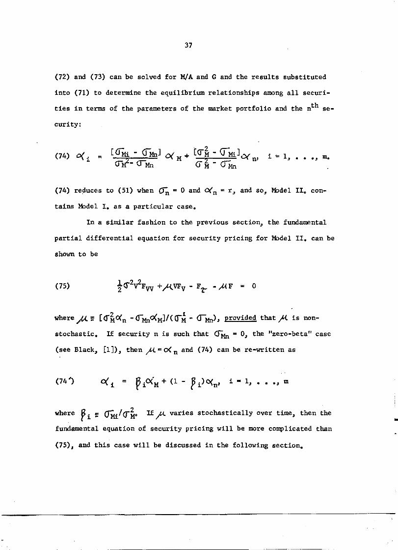A DYNAMIC GENERAL EQUDIBRIUM MODEL OF THE ASSET MARKET

AND ITS APPLICATION TO THE PRICING

OF THE CAP ITAL STRUCTURE OF THE FIRf

Robert C Merton

Massachusetts Institute of Technology November 1970

An earlier version of the paper was presented at the Conference on Capital Market Theory Massachusetts Institute of Technology July 1970 My thanks to ~~ron Scholes for helpful discussion Aid from The National Science Foundation is gratefully acknowledged

bull


















the economy as well




1

2








(1)






Z is defined by

(2) Z V(t+1)V(t)





bull

--- -------------------------------- ----shy

3

















(3)





bull

4





supplied ie







fWil 1 Fi(Vt 1



bull




5


















bull

6




tlt fc (9) e = 10 00ZdQ(Z 1)


















III

7


-It- [BV(10) e B - e-21 (B - ZV)dQ(Z7)

o












is




8



(12) =








(13) F2(VZ0) = Max[OVZ - B]7









9















ZV + nS - B




(15) 1) NS + B

10


(14) as





(17) =






(19)

bull


11
























bull

13

























tal shares will be



is

(25) F2 (V t)



o ~V ~V




e-(~+n)7 (00 VZdQ(Z 1)(27) )-rV





15






















16


(29)




n) bull













---------~---- -- shy

17













(31)


16 as

(32)



bull

18




1

k(33) d~ = w~w~ = NP 1 1 1 1 1


1



m m (34) = [ ~ (ltX l - r) + r]dt + lt wk






(35) =


fromwage income



II

19




(36)








18see [4] and [5] k





bull

20

(37)

and



risky security as





have that





21





(41) Di _ ZK d~ 1


vector form as

JI-l(4la) D == A11-1 (0( - r) + Herr





we have that -(42)


22








1


1 ~ ~


then

(44)

and hence from (42)

(45) bull


-__shy-------------------~

23



rates of return as

(46)





m (47) OCM 2 w(o( r) +r- 1 J J





24

(48)


form as

(49)















25
























bull

26






















bull

27






(52)

1t+t



(53) + ltTMX(ti 1)]



(54) ~ (t +t-)

~(t +1)


bull


28

(55)




(56) Pi criMI (r~

(2) ai = 12( ~ i (f~ -v i I

-2 C~ = 1 - PiM 0i Y i ( t 1 )












29


case is discussed




ture of the firm












dV(57) = ~ == 0( dt + CfdZ

V P



30




















31


(60)



re-write (60) as



(62)

and

(63)



(64) OC - r = -

32



(65)


to (65) is

(66)










(67)

bull


33










FvV ~e = r + --- (0(- r)

F












34


(69) dP = dV + (1 _ S )dF P V F






(70) Clte - r = ~ (0(- r)








35






















bull

36










and

(72) o(M = ~ltr2+GA M






(73) = ~ltrMn+G A

bull




37




curity

(74) 0( i = i = 1 bull bull m





shown to be

(75)



(74 )



38







(76) ~ _ r = M OmM - liS- m A A mr





(77) Oltk - r







39
















are described by




40














term structure o








bull

~---- ~--------------- shy

41



written as

dP(79) P = o(1dt + (11 dq




satisfy

Ot(80) C( - r = - (0( - r)

t- ltrm m


(81) o = ~ g2p + fP _ P 2 rr r l

and

(82) a = Prg ~ P


42













to

(84) o(k- r








bull

43





(85) P(r~ ~)
















44


























bull

45


























bull

--- ---------------~-- ----~---

46
























47

References










-


















the economy as well




1

2








(1)






Z is defined by

(2) Z V(t+1)V(t)





bull

--- -------------------------------- ----shy

3

















(3)





bull

4





supplied ie







fWil 1 Fi(Vt 1



bull




5


















bull

6




tlt fc (9) e = 10 00ZdQ(Z 1)


















III

7


-It- [BV(10) e B - e-21 (B - ZV)dQ(Z7)

o












is




8



(12) =








(13) F2(VZ0) = Max[OVZ - B]7









9















ZV + nS - B




(15) 1) NS + B

10


(14) as





(17) =






(19)

bull


11
























bull

13

























tal shares will be



is

(25) F2 (V t)



o ~V ~V




e-(~+n)7 (00 VZdQ(Z 1)(27) )-rV





15






















16


(29)




n) bull













---------~---- -- shy

17













(31)


16 as

(32)



bull

18




1

k(33) d~ = w~w~ = NP 1 1 1 1 1


1



m m (34) = [ ~ (ltX l - r) + r]dt + lt wk






(35) =


fromwage income



II

19




(36)








18see [4] and [5] k





bull

20

(37)

and



risky security as





have that





21





(41) Di _ ZK d~ 1


vector form as

JI-l(4la) D == A11-1 (0( - r) + Herr





we have that -(42)


22








1


1 ~ ~


then

(44)

and hence from (42)

(45) bull


-__shy-------------------~

23



rates of return as

(46)





m (47) OCM 2 w(o( r) +r- 1 J J





24

(48)


form as

(49)















25
























bull

26






















bull

27






(52)

1t+t



(53) + ltTMX(ti 1)]



(54) ~ (t +t-)

~(t +1)


bull


28

(55)




(56) Pi criMI (r~

(2) ai = 12( ~ i (f~ -v i I

-2 C~ = 1 - PiM 0i Y i ( t 1 )












29


case is discussed




ture of the firm












dV(57) = ~ == 0( dt + CfdZ

V P



30




















31


(60)



re-write (60) as



(62)

and

(63)



(64) OC - r = -

32



(65)


to (65) is

(66)










(67)

bull


33










FvV ~e = r + --- (0(- r)

F












34


(69) dP = dV + (1 _ S )dF P V F






(70) Clte - r = ~ (0(- r)








35






















bull

36










and

(72) o(M = ~ltr2+GA M






(73) = ~ltrMn+G A

bull




37




curity

(74) 0( i = i = 1 bull bull m





shown to be

(75)



(74 )



38







(76) ~ _ r = M OmM - liS- m A A mr





(77) Oltk - r







39
















are described by




40














term structure o








bull

~---- ~--------------- shy

41



written as

dP(79) P = o(1dt + (11 dq




satisfy

Ot(80) C( - r = - (0( - r)

t- ltrm m


(81) o = ~ g2p + fP _ P 2 rr r l

and

(82) a = Prg ~ P


42













to

(84) o(k- r








bull

43





(85) P(r~ ~)
















44


























bull

45


























bull

--- ---------------~-- ----~---

46
























47

References










-

2








(1)






Z is defined by

(2) Z V(t+1)V(t)





bull

--- -------------------------------- ----shy

3

















(3)





bull

4





supplied ie







fWil 1 Fi(Vt 1



bull




5


















bull

6




tlt fc (9) e = 10 00ZdQ(Z 1)


















III

7


-It- [BV(10) e B - e-21 (B - ZV)dQ(Z7)

o












is




8



(12) =








(13) F2(VZ0) = Max[OVZ - B]7









9















ZV + nS - B




(15) 1) NS + B

10


(14) as





(17) =






(19)

bull


11
























bull

13

























tal shares will be



is

(25) F2 (V t)



o ~V ~V




e-(~+n)7 (00 VZdQ(Z 1)(27) )-rV





15






















16


(29)




n) bull













---------~---- -- shy

17













(31)


16 as

(32)



bull

18




1

k(33) d~ = w~w~ = NP 1 1 1 1 1


1



m m (34) = [ ~ (ltX l - r) + r]dt + lt wk






(35) =


fromwage income



II

19




(36)








18see [4] and [5] k





bull

20

(37)

and



risky security as





have that





21





(41) Di _ ZK d~ 1


vector form as

JI-l(4la) D == A11-1 (0( - r) + Herr





we have that -(42)


22








1


1 ~ ~


then

(44)

and hence from (42)

(45) bull


-__shy-------------------~

23



rates of return as

(46)





m (47) OCM 2 w(o( r) +r- 1 J J





24

(48)


form as

(49)















25
























bull

26






















bull

27






(52)

1t+t



(53) + ltTMX(ti 1)]



(54) ~ (t +t-)

~(t +1)


bull


28

(55)




(56) Pi criMI (r~

(2) ai = 12( ~ i (f~ -v i I

-2 C~ = 1 - PiM 0i Y i ( t 1 )












29


case is discussed




ture of the firm












dV(57) = ~ == 0( dt + CfdZ

V P



30




















31


(60)



re-write (60) as



(62)

and

(63)



(64) OC - r = -

32



(65)


to (65) is

(66)










(67)

bull


33










FvV ~e = r + --- (0(- r)

F












34


(69) dP = dV + (1 _ S )dF P V F






(70) Clte - r = ~ (0(- r)








35






















bull

36










and

(72) o(M = ~ltr2+GA M






(73) = ~ltrMn+G A

bull




37




curity

(74) 0( i = i = 1 bull bull m





shown to be

(75)



(74 )



38







(76) ~ _ r = M OmM - liS- m A A mr





(77) Oltk - r







39
















are described by




40














term structure o








bull

~---- ~--------------- shy

41



written as

dP(79) P = o(1dt + (11 dq




satisfy

Ot(80) C( - r = - (0( - r)

t- ltrm m


(81) o = ~ g2p + fP _ P 2 rr r l

and

(82) a = Prg ~ P


42













to

(84) o(k- r








bull

43





(85) P(r~ ~)
















44


























bull

45


























bull

--- ---------------~-- ----~---

46
























47

References










-

3

















(3)





bull

4





supplied ie







fWil 1 Fi(Vt 1



bull




5


















bull

6




tlt fc (9) e = 10 00ZdQ(Z 1)


















III

7


-It- [BV(10) e B - e-21 (B - ZV)dQ(Z7)

o












is




8



(12) =








(13) F2(VZ0) = Max[OVZ - B]7









9















ZV + nS - B




(15) 1) NS + B

10


(14) as





(17) =






(19)

bull


11
























bull

13

























tal shares will be



is

(25) F2 (V t)



o ~V ~V




e-(~+n)7 (00 VZdQ(Z 1)(27) )-rV





15






















16


(29)




n) bull













---------~---- -- shy

17













(31)


16 as

(32)



bull

18




1

k(33) d~ = w~w~ = NP 1 1 1 1 1


1



m m (34) = [ ~ (ltX l - r) + r]dt + lt wk






(35) =


fromwage income



II

19




(36)








18see [4] and [5] k





bull

20

(37)

and



risky security as





have that





21





(41) Di _ ZK d~ 1


vector form as

JI-l(4la) D == A11-1 (0( - r) + Herr





we have that -(42)


22








1


1 ~ ~


then

(44)

and hence from (42)

(45) bull


-__shy-------------------~

23



rates of return as

(46)





m (47) OCM 2 w(o( r) +r- 1 J J





24

(48)


form as

(49)















25
























bull

26






















bull

27






(52)

1t+t



(53) + ltTMX(ti 1)]



(54) ~ (t +t-)

~(t +1)


bull


28

(55)




(56) Pi criMI (r~

(2) ai = 12( ~ i (f~ -v i I

-2 C~ = 1 - PiM 0i Y i ( t 1 )












29


case is discussed




ture of the firm












dV(57) = ~ == 0( dt + CfdZ

V P



30




















31


(60)



re-write (60) as



(62)

and

(63)



(64) OC - r = -

32



(65)


to (65) is

(66)










(67)

bull


33










FvV ~e = r + --- (0(- r)

F












34


(69) dP = dV + (1 _ S )dF P V F






(70) Clte - r = ~ (0(- r)








35






















bull

36










and

(72) o(M = ~ltr2+GA M






(73) = ~ltrMn+G A

bull




37




curity

(74) 0( i = i = 1 bull bull m





shown to be

(75)



(74 )



38







(76) ~ _ r = M OmM - liS- m A A mr





(77) Oltk - r







39
















are described by




40














term structure o








bull

~---- ~--------------- shy

41



written as

dP(79) P = o(1dt + (11 dq




satisfy

Ot(80) C( - r = - (0( - r)

t- ltrm m


(81) o = ~ g2p + fP _ P 2 rr r l

and

(82) a = Prg ~ P


42













to

(84) o(k- r








bull

43





(85) P(r~ ~)
















44


























bull

45


























bull

--- ---------------~-- ----~---

46
























47

References










-

4





supplied ie







fWil 1 Fi(Vt 1



bull




5


















bull

6




tlt fc (9) e = 10 00ZdQ(Z 1)


















III

7


-It- [BV(10) e B - e-21 (B - ZV)dQ(Z7)

o












is




8



(12) =








(13) F2(VZ0) = Max[OVZ - B]7









9















ZV + nS - B




(15) 1) NS + B

10


(14) as





(17) =






(19)

bull


11
























bull

13

























tal shares will be



is

(25) F2 (V t)



o ~V ~V




e-(~+n)7 (00 VZdQ(Z 1)(27) )-rV





15






















16


(29)




n) bull













---------~---- -- shy

17













(31)


16 as

(32)



bull

18




1

k(33) d~ = w~w~ = NP 1 1 1 1 1


1



m m (34) = [ ~ (ltX l - r) + r]dt + lt wk






(35) =


fromwage income



II

19




(36)








18see [4] and [5] k





bull

20

(37)

and



risky security as





have that





21





(41) Di _ ZK d~ 1


vector form as

JI-l(4la) D == A11-1 (0( - r) + Herr





we have that -(42)


22








1


1 ~ ~


then

(44)

and hence from (42)

(45) bull


-__shy-------------------~

23



rates of return as

(46)





m (47) OCM 2 w(o( r) +r- 1 J J





24

(48)


form as

(49)















25
























bull

26






















bull

27






(52)

1t+t



(53) + ltTMX(ti 1)]



(54) ~ (t +t-)

~(t +1)


bull


28

(55)




(56) Pi criMI (r~

(2) ai = 12( ~ i (f~ -v i I

-2 C~ = 1 - PiM 0i Y i ( t 1 )












29


case is discussed




ture of the firm












dV(57) = ~ == 0( dt + CfdZ

V P



30




















31


(60)



re-write (60) as



(62)

and

(63)



(64) OC - r = -

32



(65)


to (65) is

(66)










(67)

bull


33










FvV ~e = r + --- (0(- r)

F












34


(69) dP = dV + (1 _ S )dF P V F






(70) Clte - r = ~ (0(- r)








35






















bull

36










and

(72) o(M = ~ltr2+GA M






(73) = ~ltrMn+G A

bull




37




curity

(74) 0( i = i = 1 bull bull m





shown to be

(75)



(74 )



38







(76) ~ _ r = M OmM - liS- m A A mr





(77) Oltk - r







39
















are described by




40














term structure o








bull

~---- ~--------------- shy

41



written as

dP(79) P = o(1dt + (11 dq




satisfy

Ot(80) C( - r = - (0( - r)

t- ltrm m


(81) o = ~ g2p + fP _ P 2 rr r l

and

(82) a = Prg ~ P


42













to

(84) o(k- r








bull

43





(85) P(r~ ~)
















44


























bull

45


























bull

--- ---------------~-- ----~---

46
























47

References










-

5


















bull

6




tlt fc (9) e = 10 00ZdQ(Z 1)


















III

7


-It- [BV(10) e B - e-21 (B - ZV)dQ(Z7)

o












is




8



(12) =








(13) F2(VZ0) = Max[OVZ - B]7









9















ZV + nS - B




(15) 1) NS + B

10


(14) as





(17) =






(19)

bull


11
























bull

13

























tal shares will be



is

(25) F2 (V t)



o ~V ~V




e-(~+n)7 (00 VZdQ(Z 1)(27) )-rV





15






















16


(29)




n) bull













---------~---- -- shy

17













(31)


16 as

(32)



bull

18




1

k(33) d~ = w~w~ = NP 1 1 1 1 1


1



m m (34) = [ ~ (ltX l - r) + r]dt + lt wk






(35) =


fromwage income



II

19




(36)








18see [4] and [5] k





bull

20

(37)

and



risky security as





have that





21





(41) Di _ ZK d~ 1


vector form as

JI-l(4la) D == A11-1 (0( - r) + Herr





we have that -(42)


22








1


1 ~ ~


then

(44)

and hence from (42)

(45) bull


-__shy-------------------~

23



rates of return as

(46)





m (47) OCM 2 w(o( r) +r- 1 J J





24

(48)


form as

(49)















25
























bull

26






















bull

27






(52)

1t+t



(53) + ltTMX(ti 1)]



(54) ~ (t +t-)

~(t +1)


bull


28

(55)




(56) Pi criMI (r~

(2) ai = 12( ~ i (f~ -v i I

-2 C~ = 1 - PiM 0i Y i ( t 1 )












29


case is discussed




ture of the firm












dV(57) = ~ == 0( dt + CfdZ

V P



30




















31


(60)



re-write (60) as



(62)

and

(63)



(64) OC - r = -

32



(65)


to (65) is

(66)










(67)

bull


33










FvV ~e = r + --- (0(- r)

F












34


(69) dP = dV + (1 _ S )dF P V F






(70) Clte - r = ~ (0(- r)








35






















bull

36










and

(72) o(M = ~ltr2+GA M






(73) = ~ltrMn+G A

bull




37




curity

(74) 0( i = i = 1 bull bull m





shown to be

(75)



(74 )



38







(76) ~ _ r = M OmM - liS- m A A mr





(77) Oltk - r







39
















are described by




40














term structure o








bull

~---- ~--------------- shy

41



written as

dP(79) P = o(1dt + (11 dq




satisfy

Ot(80) C( - r = - (0( - r)

t- ltrm m


(81) o = ~ g2p + fP _ P 2 rr r l

and

(82) a = Prg ~ P


42













to

(84) o(k- r








bull

43





(85) P(r~ ~)
















44


























bull

45


























bull

--- ---------------~-- ----~---

46
























47

References










-

6




tlt fc (9) e = 10 00ZdQ(Z 1)


















III

7


-It- [BV(10) e B - e-21 (B - ZV)dQ(Z7)

o












is




8



(12) =








(13) F2(VZ0) = Max[OVZ - B]7









9















ZV + nS - B




(15) 1) NS + B

10


(14) as





(17) =






(19)

bull


11
























bull

13

























tal shares will be



is

(25) F2 (V t)



o ~V ~V




e-(~+n)7 (00 VZdQ(Z 1)(27) )-rV





15






















16


(29)




n) bull













---------~---- -- shy

17













(31)


16 as

(32)



bull

18




1

k(33) d~ = w~w~ = NP 1 1 1 1 1


1



m m (34) = [ ~ (ltX l - r) + r]dt + lt wk






(35) =


fromwage income



II

19




(36)








18see [4] and [5] k





bull

20

(37)

and



risky security as





have that





21





(41) Di _ ZK d~ 1


vector form as

JI-l(4la) D == A11-1 (0( - r) + Herr





we have that -(42)


22








1


1 ~ ~


then

(44)

and hence from (42)

(45) bull


-__shy-------------------~

23



rates of return as

(46)





m (47) OCM 2 w(o( r) +r- 1 J J





24

(48)


form as

(49)















25
























bull

26






















bull

27






(52)

1t+t



(53) + ltTMX(ti 1)]



(54) ~ (t +t-)

~(t +1)


bull


28

(55)




(56) Pi criMI (r~

(2) ai = 12( ~ i (f~ -v i I

-2 C~ = 1 - PiM 0i Y i ( t 1 )












29


case is discussed




ture of the firm












dV(57) = ~ == 0( dt + CfdZ

V P



30




















31


(60)



re-write (60) as



(62)

and

(63)



(64) OC - r = -

32



(65)


to (65) is

(66)










(67)

bull


33










FvV ~e = r + --- (0(- r)

F












34


(69) dP = dV + (1 _ S )dF P V F






(70) Clte - r = ~ (0(- r)








35






















bull

36










and

(72) o(M = ~ltr2+GA M






(73) = ~ltrMn+G A

bull




37




curity

(74) 0( i = i = 1 bull bull m





shown to be

(75)



(74 )



38







(76) ~ _ r = M OmM - liS- m A A mr





(77) Oltk - r







39
















are described by




40














term structure o








bull

~---- ~--------------- shy

41



written as

dP(79) P = o(1dt + (11 dq




satisfy

Ot(80) C( - r = - (0( - r)

t- ltrm m


(81) o = ~ g2p + fP _ P 2 rr r l

and

(82) a = Prg ~ P


42













to

(84) o(k- r








bull

43





(85) P(r~ ~)
















44


























bull

45


























bull

--- ---------------~-- ----~---

46
























47

References










-

7


-It- [BV(10) e B - e-21 (B - ZV)dQ(Z7)

o












is




8



(12) =








(13) F2(VZ0) = Max[OVZ - B]7









9















ZV + nS - B




(15) 1) NS + B

10


(14) as





(17) =






(19)

bull


11
























bull

13

























tal shares will be



is

(25) F2 (V t)



o ~V ~V




e-(~+n)7 (00 VZdQ(Z 1)(27) )-rV





15






















16


(29)




n) bull













---------~---- -- shy

17













(31)


16 as

(32)



bull

18




1

k(33) d~ = w~w~ = NP 1 1 1 1 1


1



m m (34) = [ ~ (ltX l - r) + r]dt + lt wk






(35) =


fromwage income



II

19




(36)








18see [4] and [5] k





bull

20

(37)

and



risky security as





have that





21





(41) Di _ ZK d~ 1


vector form as

JI-l(4la) D == A11-1 (0( - r) + Herr





we have that -(42)


22








1


1 ~ ~


then

(44)

and hence from (42)

(45) bull


-__shy-------------------~

23



rates of return as

(46)





m (47) OCM 2 w(o( r) +r- 1 J J





24

(48)


form as

(49)















25
























bull

26






















bull

27






(52)

1t+t



(53) + ltTMX(ti 1)]



(54) ~ (t +t-)

~(t +1)


bull


28

(55)




(56) Pi criMI (r~

(2) ai = 12( ~ i (f~ -v i I

-2 C~ = 1 - PiM 0i Y i ( t 1 )












29


case is discussed




ture of the firm












dV(57) = ~ == 0( dt + CfdZ

V P



30




















31


(60)



re-write (60) as



(62)

and

(63)



(64) OC - r = -

32



(65)


to (65) is

(66)










(67)

bull


33










FvV ~e = r + --- (0(- r)

F












34


(69) dP = dV + (1 _ S )dF P V F






(70) Clte - r = ~ (0(- r)








35






















bull

36










and

(72) o(M = ~ltr2+GA M






(73) = ~ltrMn+G A

bull




37




curity

(74) 0( i = i = 1 bull bull m





shown to be

(75)



(74 )



38







(76) ~ _ r = M OmM - liS- m A A mr





(77) Oltk - r







39
















are described by




40














term structure o








bull

~---- ~--------------- shy

41



written as

dP(79) P = o(1dt + (11 dq




satisfy

Ot(80) C( - r = - (0( - r)

t- ltrm m


(81) o = ~ g2p + fP _ P 2 rr r l

and

(82) a = Prg ~ P


42













to

(84) o(k- r








bull

43





(85) P(r~ ~)
















44


























bull

45


























bull

--- ---------------~-- ----~---

46
























47

References










-

8



(12) =








(13) F2(VZ0) = Max[OVZ - B]7









9















ZV + nS - B




(15) 1) NS + B

10


(14) as





(17) =






(19)

bull


11
























bull

13

























tal shares will be



is

(25) F2 (V t)



o ~V ~V




e-(~+n)7 (00 VZdQ(Z 1)(27) )-rV





15






















16


(29)




n) bull













---------~---- -- shy

17













(31)


16 as

(32)



bull

18




1

k(33) d~ = w~w~ = NP 1 1 1 1 1


1



m m (34) = [ ~ (ltX l - r) + r]dt + lt wk






(35) =


fromwage income



II

19




(36)








18see [4] and [5] k





bull

20

(37)

and



risky security as





have that





21





(41) Di _ ZK d~ 1


vector form as

JI-l(4la) D == A11-1 (0( - r) + Herr





we have that -(42)


22








1


1 ~ ~


then

(44)

and hence from (42)

(45) bull


-__shy-------------------~

23



rates of return as

(46)





m (47) OCM 2 w(o( r) +r- 1 J J





24

(48)


form as

(49)















25
























bull

26






















bull

27






(52)

1t+t



(53) + ltTMX(ti 1)]



(54) ~ (t +t-)

~(t +1)


bull


28

(55)




(56) Pi criMI (r~

(2) ai = 12( ~ i (f~ -v i I

-2 C~ = 1 - PiM 0i Y i ( t 1 )












29


case is discussed




ture of the firm












dV(57) = ~ == 0( dt + CfdZ

V P



30




















31


(60)



re-write (60) as



(62)

and

(63)



(64) OC - r = -

32



(65)


to (65) is

(66)










(67)

bull


33










FvV ~e = r + --- (0(- r)

F












34


(69) dP = dV + (1 _ S )dF P V F






(70) Clte - r = ~ (0(- r)








35






















bull

36










and

(72) o(M = ~ltr2+GA M






(73) = ~ltrMn+G A

bull




37




curity

(74) 0( i = i = 1 bull bull m





shown to be

(75)



(74 )



38







(76) ~ _ r = M OmM - liS- m A A mr





(77) Oltk - r







39
















are described by




40














term structure o








bull

~---- ~--------------- shy

41



written as

dP(79) P = o(1dt + (11 dq




satisfy

Ot(80) C( - r = - (0( - r)

t- ltrm m


(81) o = ~ g2p + fP _ P 2 rr r l

and

(82) a = Prg ~ P


42













to

(84) o(k- r








bull

43





(85) P(r~ ~)
















44


























bull

45


























bull

--- ---------------~-- ----~---

46
























47

References










-

9















ZV + nS - B




(15) 1) NS + B

10


(14) as





(17) =






(19)

bull


11
























bull

13

























tal shares will be



is

(25) F2 (V t)



o ~V ~V




e-(~+n)7 (00 VZdQ(Z 1)(27) )-rV





15






















16


(29)




n) bull













---------~---- -- shy

17













(31)


16 as

(32)



bull

18




1

k(33) d~ = w~w~ = NP 1 1 1 1 1


1



m m (34) = [ ~ (ltX l - r) + r]dt + lt wk






(35) =


fromwage income



II

19




(36)








18see [4] and [5] k





bull

20

(37)

and



risky security as





have that





21





(41) Di _ ZK d~ 1


vector form as

JI-l(4la) D == A11-1 (0( - r) + Herr





we have that -(42)


22








1


1 ~ ~


then

(44)

and hence from (42)

(45) bull


-__shy-------------------~

23



rates of return as

(46)





m (47) OCM 2 w(o( r) +r- 1 J J





24

(48)


form as

(49)















25
























bull

26






















bull

27






(52)

1t+t



(53) + ltTMX(ti 1)]



(54) ~ (t +t-)

~(t +1)


bull


28

(55)




(56) Pi criMI (r~

(2) ai = 12( ~ i (f~ -v i I

-2 C~ = 1 - PiM 0i Y i ( t 1 )












29


case is discussed




ture of the firm












dV(57) = ~ == 0( dt + CfdZ

V P



30




















31


(60)



re-write (60) as



(62)

and

(63)



(64) OC - r = -

32



(65)


to (65) is

(66)










(67)

bull


33










FvV ~e = r + --- (0(- r)

F












34


(69) dP = dV + (1 _ S )dF P V F






(70) Clte - r = ~ (0(- r)








35






















bull

36










and

(72) o(M = ~ltr2+GA M






(73) = ~ltrMn+G A

bull




37




curity

(74) 0( i = i = 1 bull bull m





shown to be

(75)



(74 )



38







(76) ~ _ r = M OmM - liS- m A A mr





(77) Oltk - r







39
















are described by




40














term structure o








bull

~---- ~--------------- shy

41



written as

dP(79) P = o(1dt + (11 dq




satisfy

Ot(80) C( - r = - (0( - r)

t- ltrm m


(81) o = ~ g2p + fP _ P 2 rr r l

and

(82) a = Prg ~ P


42













to

(84) o(k- r








bull

43





(85) P(r~ ~)
















44


























bull

45


























bull

--- ---------------~-- ----~---

46
























47

References










-

10


(14) as





(17) =






(19)

bull


11
























bull

13

























tal shares will be



is

(25) F2 (V t)



o ~V ~V




e-(~+n)7 (00 VZdQ(Z 1)(27) )-rV





15






















16


(29)




n) bull













---------~---- -- shy

17













(31)


16 as

(32)



bull

18




1

k(33) d~ = w~w~ = NP 1 1 1 1 1


1



m m (34) = [ ~ (ltX l - r) + r]dt + lt wk






(35) =


fromwage income



II

19




(36)








18see [4] and [5] k





bull

20

(37)

and



risky security as





have that





21





(41) Di _ ZK d~ 1


vector form as

JI-l(4la) D == A11-1 (0( - r) + Herr





we have that -(42)


22








1


1 ~ ~


then

(44)

and hence from (42)

(45) bull


-__shy-------------------~

23



rates of return as

(46)





m (47) OCM 2 w(o( r) +r- 1 J J





24

(48)


form as

(49)















25
























bull

26






















bull

27






(52)

1t+t



(53) + ltTMX(ti 1)]



(54) ~ (t +t-)

~(t +1)


bull


28

(55)




(56) Pi criMI (r~

(2) ai = 12( ~ i (f~ -v i I

-2 C~ = 1 - PiM 0i Y i ( t 1 )












29


case is discussed




ture of the firm












dV(57) = ~ == 0( dt + CfdZ

V P



30




















31


(60)



re-write (60) as



(62)

and

(63)



(64) OC - r = -

32



(65)


to (65) is

(66)










(67)

bull


33










FvV ~e = r + --- (0(- r)

F












34


(69) dP = dV + (1 _ S )dF P V F






(70) Clte - r = ~ (0(- r)








35






















bull

36










and

(72) o(M = ~ltr2+GA M






(73) = ~ltrMn+G A

bull




37




curity

(74) 0( i = i = 1 bull bull m





shown to be

(75)



(74 )



38







(76) ~ _ r = M OmM - liS- m A A mr





(77) Oltk - r







39
















are described by




40














term structure o








bull

~---- ~--------------- shy

41



written as

dP(79) P = o(1dt + (11 dq




satisfy

Ot(80) C( - r = - (0( - r)

t- ltrm m


(81) o = ~ g2p + fP _ P 2 rr r l

and

(82) a = Prg ~ P


42













to

(84) o(k- r








bull

43





(85) P(r~ ~)
















44


























bull

45


























bull

--- ---------------~-- ----~---

46
























47

References










-

11
























bull

13

























tal shares will be



is

(25) F2 (V t)



o ~V ~V




e-(~+n)7 (00 VZdQ(Z 1)(27) )-rV





15






















16


(29)




n) bull













---------~---- -- shy

17













(31)


16 as

(32)



bull

18




1

k(33) d~ = w~w~ = NP 1 1 1 1 1


1



m m (34) = [ ~ (ltX l - r) + r]dt + lt wk






(35) =


fromwage income



II

19




(36)








18see [4] and [5] k





bull

20

(37)

and



risky security as





have that





21





(41) Di _ ZK d~ 1


vector form as

JI-l(4la) D == A11-1 (0( - r) + Herr





we have that -(42)


22








1


1 ~ ~


then

(44)

and hence from (42)

(45) bull


-__shy-------------------~

23



rates of return as

(46)





m (47) OCM 2 w(o( r) +r- 1 J J





24

(48)


form as

(49)















25
























bull

26






















bull

27






(52)

1t+t



(53) + ltTMX(ti 1)]



(54) ~ (t +t-)

~(t +1)


bull


28

(55)




(56) Pi criMI (r~

(2) ai = 12( ~ i (f~ -v i I

-2 C~ = 1 - PiM 0i Y i ( t 1 )












29


case is discussed




ture of the firm












dV(57) = ~ == 0( dt + CfdZ

V P



30




















31


(60)



re-write (60) as



(62)

and

(63)



(64) OC - r = -

32



(65)


to (65) is

(66)










(67)

bull


33










FvV ~e = r + --- (0(- r)

F












34


(69) dP = dV + (1 _ S )dF P V F






(70) Clte - r = ~ (0(- r)








35






















bull

36










and

(72) o(M = ~ltr2+GA M






(73) = ~ltrMn+G A

bull




37




curity

(74) 0( i = i = 1 bull bull m





shown to be

(75)



(74 )



38







(76) ~ _ r = M OmM - liS- m A A mr





(77) Oltk - r







39
















are described by




40














term structure o








bull

~---- ~--------------- shy

41



written as

dP(79) P = o(1dt + (11 dq




satisfy

Ot(80) C( - r = - (0( - r)

t- ltrm m


(81) o = ~ g2p + fP _ P 2 rr r l

and

(82) a = Prg ~ P


42













to

(84) o(k- r








bull

43





(85) P(r~ ~)
















44


























bull

45


























bull

--- ---------------~-- ----~---

46
























47

References










-

13

























tal shares will be



is

(25) F2 (V t)



o ~V ~V




e-(~+n)7 (00 VZdQ(Z 1)(27) )-rV





15






















16


(29)




n) bull













---------~---- -- shy

17













(31)


16 as

(32)



bull

18




1

k(33) d~ = w~w~ = NP 1 1 1 1 1


1



m m (34) = [ ~ (ltX l - r) + r]dt + lt wk






(35) =


fromwage income



II

19




(36)








18see [4] and [5] k





bull

20

(37)

and



risky security as





have that





21





(41) Di _ ZK d~ 1


vector form as

JI-l(4la) D == A11-1 (0( - r) + Herr





we have that -(42)


22








1


1 ~ ~


then

(44)

and hence from (42)

(45) bull


-__shy-------------------~

23



rates of return as

(46)





m (47) OCM 2 w(o( r) +r- 1 J J





24

(48)


form as

(49)















25
























bull

26






















bull

27






(52)

1t+t



(53) + ltTMX(ti 1)]



(54) ~ (t +t-)

~(t +1)


bull


28

(55)




(56) Pi criMI (r~

(2) ai = 12( ~ i (f~ -v i I

-2 C~ = 1 - PiM 0i Y i ( t 1 )












29


case is discussed




ture of the firm












dV(57) = ~ == 0( dt + CfdZ

V P



30




















31


(60)



re-write (60) as



(62)

and

(63)



(64) OC - r = -

32



(65)


to (65) is

(66)










(67)

bull


33










FvV ~e = r + --- (0(- r)

F












34


(69) dP = dV + (1 _ S )dF P V F






(70) Clte - r = ~ (0(- r)








35






















bull

36










and

(72) o(M = ~ltr2+GA M






(73) = ~ltrMn+G A

bull




37




curity

(74) 0( i = i = 1 bull bull m





shown to be

(75)



(74 )



38







(76) ~ _ r = M OmM - liS- m A A mr





(77) Oltk - r







39
















are described by




40














term structure o








bull

~---- ~--------------- shy

41



written as

dP(79) P = o(1dt + (11 dq




satisfy

Ot(80) C( - r = - (0( - r)

t- ltrm m


(81) o = ~ g2p + fP _ P 2 rr r l

and

(82) a = Prg ~ P


42













to

(84) o(k- r








bull

43





(85) P(r~ ~)
















44


























bull

45


























bull

--- ---------------~-- ----~---

46
























47

References










-



is

(25) F2 (V t)



o ~V ~V




e-(~+n)7 (00 VZdQ(Z 1)(27) )-rV





15






















16


(29)




n) bull













---------~---- -- shy

17













(31)


16 as

(32)



bull

18




1

k(33) d~ = w~w~ = NP 1 1 1 1 1


1



m m (34) = [ ~ (ltX l - r) + r]dt + lt wk






(35) =


fromwage income



II

19




(36)








18see [4] and [5] k





bull

20

(37)

and



risky security as





have that





21





(41) Di _ ZK d~ 1


vector form as

JI-l(4la) D == A11-1 (0( - r) + Herr





we have that -(42)


22








1


1 ~ ~


then

(44)

and hence from (42)

(45) bull


-__shy-------------------~

23



rates of return as

(46)





m (47) OCM 2 w(o( r) +r- 1 J J





24

(48)


form as

(49)















25
























bull

26






















bull

27






(52)

1t+t



(53) + ltTMX(ti 1)]



(54) ~ (t +t-)

~(t +1)


bull


28

(55)




(56) Pi criMI (r~

(2) ai = 12( ~ i (f~ -v i I

-2 C~ = 1 - PiM 0i Y i ( t 1 )












29


case is discussed




ture of the firm












dV(57) = ~ == 0( dt + CfdZ

V P



30




















31


(60)



re-write (60) as



(62)

and

(63)



(64) OC - r = -

32



(65)


to (65) is

(66)










(67)

bull


33










FvV ~e = r + --- (0(- r)

F












34


(69) dP = dV + (1 _ S )dF P V F






(70) Clte - r = ~ (0(- r)








35






















bull

36










and

(72) o(M = ~ltr2+GA M






(73) = ~ltrMn+G A

bull




37




curity

(74) 0( i = i = 1 bull bull m





shown to be

(75)



(74 )



38







(76) ~ _ r = M OmM - liS- m A A mr





(77) Oltk - r







39
















are described by




40














term structure o








bull

~---- ~--------------- shy

41



written as

dP(79) P = o(1dt + (11 dq




satisfy

Ot(80) C( - r = - (0( - r)

t- ltrm m


(81) o = ~ g2p + fP _ P 2 rr r l

and

(82) a = Prg ~ P


42













to

(84) o(k- r








bull

43





(85) P(r~ ~)
















44


























bull

45


























bull

--- ---------------~-- ----~---

46
























47

References










-

15






















16


(29)




n) bull













---------~---- -- shy

17













(31)


16 as

(32)



bull

18




1

k(33) d~ = w~w~ = NP 1 1 1 1 1


1



m m (34) = [ ~ (ltX l - r) + r]dt + lt wk






(35) =


fromwage income



II

19




(36)








18see [4] and [5] k





bull

20

(37)

and



risky security as





have that





21





(41) Di _ ZK d~ 1


vector form as

JI-l(4la) D == A11-1 (0( - r) + Herr





we have that -(42)


22








1


1 ~ ~


then

(44)

and hence from (42)

(45) bull


-__shy-------------------~

23



rates of return as

(46)





m (47) OCM 2 w(o( r) +r- 1 J J





24

(48)


form as

(49)















25
























bull

26






















bull

27






(52)

1t+t



(53) + ltTMX(ti 1)]



(54) ~ (t +t-)

~(t +1)


bull


28

(55)




(56) Pi criMI (r~

(2) ai = 12( ~ i (f~ -v i I

-2 C~ = 1 - PiM 0i Y i ( t 1 )












29


case is discussed




ture of the firm












dV(57) = ~ == 0( dt + CfdZ

V P



30




















31


(60)



re-write (60) as



(62)

and

(63)



(64) OC - r = -

32



(65)


to (65) is

(66)










(67)

bull


33










FvV ~e = r + --- (0(- r)

F












34


(69) dP = dV + (1 _ S )dF P V F






(70) Clte - r = ~ (0(- r)








35






















bull

36










and

(72) o(M = ~ltr2+GA M






(73) = ~ltrMn+G A

bull




37




curity

(74) 0( i = i = 1 bull bull m





shown to be

(75)



(74 )



38







(76) ~ _ r = M OmM - liS- m A A mr





(77) Oltk - r







39
















are described by




40














term structure o








bull

~---- ~--------------- shy

41



written as

dP(79) P = o(1dt + (11 dq




satisfy

Ot(80) C( - r = - (0( - r)

t- ltrm m


(81) o = ~ g2p + fP _ P 2 rr r l

and

(82) a = Prg ~ P


42













to

(84) o(k- r








bull

43





(85) P(r~ ~)
















44


























bull

45


























bull

--- ---------------~-- ----~---

46
























47

References










-

16


(29)




n) bull













---------~---- -- shy

17













(31)


16 as

(32)



bull

18




1

k(33) d~ = w~w~ = NP 1 1 1 1 1


1



m m (34) = [ ~ (ltX l - r) + r]dt + lt wk






(35) =


fromwage income



II

19




(36)








18see [4] and [5] k





bull

20

(37)

and



risky security as





have that





21





(41) Di _ ZK d~ 1


vector form as

JI-l(4la) D == A11-1 (0( - r) + Herr





we have that -(42)


22








1


1 ~ ~


then

(44)

and hence from (42)

(45) bull


-__shy-------------------~

23



rates of return as

(46)





m (47) OCM 2 w(o( r) +r- 1 J J





24

(48)


form as

(49)















25
























bull

26






















bull

27






(52)

1t+t



(53) + ltTMX(ti 1)]



(54) ~ (t +t-)

~(t +1)


bull


28

(55)




(56) Pi criMI (r~

(2) ai = 12( ~ i (f~ -v i I

-2 C~ = 1 - PiM 0i Y i ( t 1 )












29


case is discussed




ture of the firm












dV(57) = ~ == 0( dt + CfdZ

V P



30




















31


(60)



re-write (60) as



(62)

and

(63)



(64) OC - r = -

32



(65)


to (65) is

(66)










(67)

bull


33










FvV ~e = r + --- (0(- r)

F












34


(69) dP = dV + (1 _ S )dF P V F






(70) Clte - r = ~ (0(- r)








35






















bull

36










and

(72) o(M = ~ltr2+GA M






(73) = ~ltrMn+G A

bull




37




curity

(74) 0( i = i = 1 bull bull m





shown to be

(75)



(74 )



38







(76) ~ _ r = M OmM - liS- m A A mr





(77) Oltk - r







39
















are described by




40














term structure o








bull

~---- ~--------------- shy

41



written as

dP(79) P = o(1dt + (11 dq




satisfy

Ot(80) C( - r = - (0( - r)

t- ltrm m


(81) o = ~ g2p + fP _ P 2 rr r l

and

(82) a = Prg ~ P


42













to

(84) o(k- r








bull

43





(85) P(r~ ~)
















44


























bull

45


























bull

--- ---------------~-- ----~---

46
























47

References










-

17













(31)


16 as

(32)



bull

18




1

k(33) d~ = w~w~ = NP 1 1 1 1 1


1



m m (34) = [ ~ (ltX l - r) + r]dt + lt wk






(35) =


fromwage income



II

19




(36)








18see [4] and [5] k





bull

20

(37)

and



risky security as





have that





21





(41) Di _ ZK d~ 1


vector form as

JI-l(4la) D == A11-1 (0( - r) + Herr





we have that -(42)


22








1


1 ~ ~


then

(44)

and hence from (42)

(45) bull


-__shy-------------------~

23



rates of return as

(46)





m (47) OCM 2 w(o( r) +r- 1 J J





24

(48)


form as

(49)















25
























bull

26






















bull

27






(52)

1t+t



(53) + ltTMX(ti 1)]



(54) ~ (t +t-)

~(t +1)


bull


28

(55)




(56) Pi criMI (r~

(2) ai = 12( ~ i (f~ -v i I

-2 C~ = 1 - PiM 0i Y i ( t 1 )












29


case is discussed




ture of the firm












dV(57) = ~ == 0( dt + CfdZ

V P



30




















31


(60)



re-write (60) as



(62)

and

(63)



(64) OC - r = -

32



(65)


to (65) is

(66)










(67)

bull


33










FvV ~e = r + --- (0(- r)

F












34


(69) dP = dV + (1 _ S )dF P V F






(70) Clte - r = ~ (0(- r)








35






















bull

36










and

(72) o(M = ~ltr2+GA M






(73) = ~ltrMn+G A

bull




37




curity

(74) 0( i = i = 1 bull bull m





shown to be

(75)



(74 )



38







(76) ~ _ r = M OmM - liS- m A A mr





(77) Oltk - r







39
















are described by




40














term structure o








bull

~---- ~--------------- shy

41



written as

dP(79) P = o(1dt + (11 dq




satisfy

Ot(80) C( - r = - (0( - r)

t- ltrm m


(81) o = ~ g2p + fP _ P 2 rr r l

and

(82) a = Prg ~ P


42













to

(84) o(k- r








bull

43





(85) P(r~ ~)
















44


























bull

45


























bull

--- ---------------~-- ----~---

46
























47

References










-

18




1

k(33) d~ = w~w~ = NP 1 1 1 1 1


1



m m (34) = [ ~ (ltX l - r) + r]dt + lt wk






(35) =


fromwage income



II

19




(36)








18see [4] and [5] k





bull

20

(37)

and



risky security as





have that





21





(41) Di _ ZK d~ 1


vector form as

JI-l(4la) D == A11-1 (0( - r) + Herr





we have that -(42)


22








1


1 ~ ~


then

(44)

and hence from (42)

(45) bull


-__shy-------------------~

23



rates of return as

(46)





m (47) OCM 2 w(o( r) +r- 1 J J





24

(48)


form as

(49)















25
























bull

26






















bull

27






(52)

1t+t



(53) + ltTMX(ti 1)]



(54) ~ (t +t-)

~(t +1)


bull


28

(55)




(56) Pi criMI (r~

(2) ai = 12( ~ i (f~ -v i I

-2 C~ = 1 - PiM 0i Y i ( t 1 )












29


case is discussed




ture of the firm












dV(57) = ~ == 0( dt + CfdZ

V P



30




















31


(60)



re-write (60) as



(62)

and

(63)



(64) OC - r = -

32



(65)


to (65) is

(66)










(67)

bull


33










FvV ~e = r + --- (0(- r)

F












34


(69) dP = dV + (1 _ S )dF P V F






(70) Clte - r = ~ (0(- r)








35






















bull

36










and

(72) o(M = ~ltr2+GA M






(73) = ~ltrMn+G A

bull




37




curity

(74) 0( i = i = 1 bull bull m





shown to be

(75)



(74 )



38







(76) ~ _ r = M OmM - liS- m A A mr





(77) Oltk - r







39
















are described by




40














term structure o








bull

~---- ~--------------- shy

41



written as

dP(79) P = o(1dt + (11 dq




satisfy

Ot(80) C( - r = - (0( - r)

t- ltrm m


(81) o = ~ g2p + fP _ P 2 rr r l

and

(82) a = Prg ~ P


42













to

(84) o(k- r








bull

43





(85) P(r~ ~)
















44


























bull

45


























bull

--- ---------------~-- ----~---

46
























47

References










-

19




(36)








18see [4] and [5] k





bull

20

(37)

and



risky security as





have that





21





(41) Di _ ZK d~ 1


vector form as

JI-l(4la) D == A11-1 (0( - r) + Herr





we have that -(42)


22








1


1 ~ ~


then

(44)

and hence from (42)

(45) bull


-__shy-------------------~

23



rates of return as

(46)





m (47) OCM 2 w(o( r) +r- 1 J J





24

(48)


form as

(49)















25
























bull

26






















bull

27






(52)

1t+t



(53) + ltTMX(ti 1)]



(54) ~ (t +t-)

~(t +1)


bull


28

(55)




(56) Pi criMI (r~

(2) ai = 12( ~ i (f~ -v i I

-2 C~ = 1 - PiM 0i Y i ( t 1 )












29


case is discussed




ture of the firm












dV(57) = ~ == 0( dt + CfdZ

V P



30




















31


(60)



re-write (60) as



(62)

and

(63)



(64) OC - r = -

32



(65)


to (65) is

(66)










(67)

bull


33










FvV ~e = r + --- (0(- r)

F












34


(69) dP = dV + (1 _ S )dF P V F






(70) Clte - r = ~ (0(- r)








35






















bull

36










and

(72) o(M = ~ltr2+GA M






(73) = ~ltrMn+G A

bull




37




curity

(74) 0( i = i = 1 bull bull m





shown to be

(75)



(74 )



38







(76) ~ _ r = M OmM - liS- m A A mr





(77) Oltk - r







39
















are described by




40














term structure o








bull

~---- ~--------------- shy

41



written as

dP(79) P = o(1dt + (11 dq




satisfy

Ot(80) C( - r = - (0( - r)

t- ltrm m


(81) o = ~ g2p + fP _ P 2 rr r l

and

(82) a = Prg ~ P


42













to

(84) o(k- r








bull

43





(85) P(r~ ~)
















44


























bull

45


























bull

--- ---------------~-- ----~---

46
























47

References










-

20

(37)

and



risky security as





have that





21





(41) Di _ ZK d~ 1


vector form as

JI-l(4la) D == A11-1 (0( - r) + Herr





we have that -(42)


22








1


1 ~ ~


then

(44)

and hence from (42)

(45) bull


-__shy-------------------~

23



rates of return as

(46)





m (47) OCM 2 w(o( r) +r- 1 J J





24

(48)


form as

(49)















25
























bull

26






















bull

27






(52)

1t+t



(53) + ltTMX(ti 1)]



(54) ~ (t +t-)

~(t +1)


bull


28

(55)




(56) Pi criMI (r~

(2) ai = 12( ~ i (f~ -v i I

-2 C~ = 1 - PiM 0i Y i ( t 1 )












29


case is discussed




ture of the firm












dV(57) = ~ == 0( dt + CfdZ

V P



30




















31


(60)



re-write (60) as



(62)

and

(63)



(64) OC - r = -

32



(65)


to (65) is

(66)










(67)

bull


33










FvV ~e = r + --- (0(- r)

F












34


(69) dP = dV + (1 _ S )dF P V F






(70) Clte - r = ~ (0(- r)








35






















bull

36










and

(72) o(M = ~ltr2+GA M






(73) = ~ltrMn+G A

bull




37




curity

(74) 0( i = i = 1 bull bull m





shown to be

(75)



(74 )



38







(76) ~ _ r = M OmM - liS- m A A mr





(77) Oltk - r







39
















are described by




40














term structure o








bull

~---- ~--------------- shy

41



written as

dP(79) P = o(1dt + (11 dq




satisfy

Ot(80) C( - r = - (0( - r)

t- ltrm m


(81) o = ~ g2p + fP _ P 2 rr r l

and

(82) a = Prg ~ P


42













to

(84) o(k- r








bull

43





(85) P(r~ ~)
















44


























bull

45


























bull

--- ---------------~-- ----~---

46
























47

References










-

21





(41) Di _ ZK d~ 1


vector form as

JI-l(4la) D == A11-1 (0( - r) + Herr





we have that -(42)


22








1


1 ~ ~


then

(44)

and hence from (42)

(45) bull


-__shy-------------------~

23



rates of return as

(46)





m (47) OCM 2 w(o( r) +r- 1 J J





24

(48)


form as

(49)















25
























bull

26






















bull

27






(52)

1t+t



(53) + ltTMX(ti 1)]



(54) ~ (t +t-)

~(t +1)


bull


28

(55)




(56) Pi criMI (r~

(2) ai = 12( ~ i (f~ -v i I

-2 C~ = 1 - PiM 0i Y i ( t 1 )












29


case is discussed




ture of the firm












dV(57) = ~ == 0( dt + CfdZ

V P



30




















31


(60)



re-write (60) as



(62)

and

(63)



(64) OC - r = -

32



(65)


to (65) is

(66)










(67)

bull


33










FvV ~e = r + --- (0(- r)

F












34


(69) dP = dV + (1 _ S )dF P V F






(70) Clte - r = ~ (0(- r)








35






















bull

36










and

(72) o(M = ~ltr2+GA M






(73) = ~ltrMn+G A

bull




37




curity

(74) 0( i = i = 1 bull bull m





shown to be

(75)



(74 )



38







(76) ~ _ r = M OmM - liS- m A A mr





(77) Oltk - r







39
















are described by




40














term structure o








bull

~---- ~--------------- shy

41



written as

dP(79) P = o(1dt + (11 dq




satisfy

Ot(80) C( - r = - (0( - r)

t- ltrm m


(81) o = ~ g2p + fP _ P 2 rr r l

and

(82) a = Prg ~ P


42













to

(84) o(k- r








bull

43





(85) P(r~ ~)
















44


























bull

45


























bull

--- ---------------~-- ----~---

46
























47

References










-

22








1


1 ~ ~


then

(44)

and hence from (42)

(45) bull


-__shy-------------------~

23



rates of return as

(46)





m (47) OCM 2 w(o( r) +r- 1 J J





24

(48)


form as

(49)















25
























bull

26






















bull

27






(52)

1t+t



(53) + ltTMX(ti 1)]



(54) ~ (t +t-)

~(t +1)


bull


28

(55)




(56) Pi criMI (r~

(2) ai = 12( ~ i (f~ -v i I

-2 C~ = 1 - PiM 0i Y i ( t 1 )












29


case is discussed




ture of the firm












dV(57) = ~ == 0( dt + CfdZ

V P



30




















31


(60)



re-write (60) as



(62)

and

(63)



(64) OC - r = -

32



(65)


to (65) is

(66)










(67)

bull


33










FvV ~e = r + --- (0(- r)

F












34


(69) dP = dV + (1 _ S )dF P V F






(70) Clte - r = ~ (0(- r)








35






















bull

36










and

(72) o(M = ~ltr2+GA M






(73) = ~ltrMn+G A

bull




37




curity

(74) 0( i = i = 1 bull bull m





shown to be

(75)



(74 )



38







(76) ~ _ r = M OmM - liS- m A A mr





(77) Oltk - r







39
















are described by




40














term structure o








bull

~---- ~--------------- shy

41



written as

dP(79) P = o(1dt + (11 dq




satisfy

Ot(80) C( - r = - (0( - r)

t- ltrm m


(81) o = ~ g2p + fP _ P 2 rr r l

and

(82) a = Prg ~ P


42













to

(84) o(k- r








bull

43





(85) P(r~ ~)
















44


























bull

45


























bull

--- ---------------~-- ----~---

46
























47

References










-

23



rates of return as

(46)





m (47) OCM 2 w(o( r) +r- 1 J J





24

(48)


form as

(49)















25
























bull

26






















bull

27






(52)

1t+t



(53) + ltTMX(ti 1)]



(54) ~ (t +t-)

~(t +1)


bull


28

(55)




(56) Pi criMI (r~

(2) ai = 12( ~ i (f~ -v i I

-2 C~ = 1 - PiM 0i Y i ( t 1 )












29


case is discussed




ture of the firm












dV(57) = ~ == 0( dt + CfdZ

V P



30




















31


(60)



re-write (60) as



(62)

and

(63)



(64) OC - r = -

32



(65)


to (65) is

(66)










(67)

bull


33










FvV ~e = r + --- (0(- r)

F












34


(69) dP = dV + (1 _ S )dF P V F






(70) Clte - r = ~ (0(- r)








35






















bull

36










and

(72) o(M = ~ltr2+GA M






(73) = ~ltrMn+G A

bull




37




curity

(74) 0( i = i = 1 bull bull m





shown to be

(75)



(74 )



38







(76) ~ _ r = M OmM - liS- m A A mr





(77) Oltk - r







39
















are described by




40














term structure o








bull

~---- ~--------------- shy

41



written as

dP(79) P = o(1dt + (11 dq




satisfy

Ot(80) C( - r = - (0( - r)

t- ltrm m


(81) o = ~ g2p + fP _ P 2 rr r l

and

(82) a = Prg ~ P


42













to

(84) o(k- r








bull

43





(85) P(r~ ~)
















44


























bull

45


























bull

--- ---------------~-- ----~---

46
























47

References










-

24

(48)


form as

(49)















25
























bull

26






















bull

27






(52)

1t+t



(53) + ltTMX(ti 1)]



(54) ~ (t +t-)

~(t +1)


bull


28

(55)




(56) Pi criMI (r~

(2) ai = 12( ~ i (f~ -v i I

-2 C~ = 1 - PiM 0i Y i ( t 1 )












29


case is discussed




ture of the firm












dV(57) = ~ == 0( dt + CfdZ

V P



30




















31


(60)



re-write (60) as



(62)

and

(63)



(64) OC - r = -

32



(65)


to (65) is

(66)










(67)

bull


33










FvV ~e = r + --- (0(- r)

F












34


(69) dP = dV + (1 _ S )dF P V F






(70) Clte - r = ~ (0(- r)








35






















bull

36










and

(72) o(M = ~ltr2+GA M






(73) = ~ltrMn+G A

bull




37




curity

(74) 0( i = i = 1 bull bull m





shown to be

(75)



(74 )



38







(76) ~ _ r = M OmM - liS- m A A mr





(77) Oltk - r







39
















are described by




40














term structure o








bull

~---- ~--------------- shy

41



written as

dP(79) P = o(1dt + (11 dq




satisfy

Ot(80) C( - r = - (0( - r)

t- ltrm m


(81) o = ~ g2p + fP _ P 2 rr r l

and

(82) a = Prg ~ P


42













to

(84) o(k- r








bull

43





(85) P(r~ ~)
















44


























bull

45


























bull

--- ---------------~-- ----~---

46
























47

References










-

25
























bull

26






















bull

27






(52)

1t+t



(53) + ltTMX(ti 1)]



(54) ~ (t +t-)

~(t +1)


bull


28

(55)




(56) Pi criMI (r~

(2) ai = 12( ~ i (f~ -v i I

-2 C~ = 1 - PiM 0i Y i ( t 1 )












29


case is discussed




ture of the firm












dV(57) = ~ == 0( dt + CfdZ

V P



30




















31


(60)



re-write (60) as



(62)

and

(63)



(64) OC - r = -

32



(65)


to (65) is

(66)










(67)

bull


33










FvV ~e = r + --- (0(- r)

F












34


(69) dP = dV + (1 _ S )dF P V F






(70) Clte - r = ~ (0(- r)








35






















bull

36










and

(72) o(M = ~ltr2+GA M






(73) = ~ltrMn+G A

bull




37




curity

(74) 0( i = i = 1 bull bull m





shown to be

(75)



(74 )



38







(76) ~ _ r = M OmM - liS- m A A mr





(77) Oltk - r







39
















are described by




40














term structure o








bull

~---- ~--------------- shy

41



written as

dP(79) P = o(1dt + (11 dq




satisfy

Ot(80) C( - r = - (0( - r)

t- ltrm m


(81) o = ~ g2p + fP _ P 2 rr r l

and

(82) a = Prg ~ P


42













to

(84) o(k- r








bull

43





(85) P(r~ ~)
















44


























bull

45


























bull

--- ---------------~-- ----~---

46
























47

References










-

26






















bull

27






(52)

1t+t



(53) + ltTMX(ti 1)]



(54) ~ (t +t-)

~(t +1)


bull


28

(55)




(56) Pi criMI (r~

(2) ai = 12( ~ i (f~ -v i I

-2 C~ = 1 - PiM 0i Y i ( t 1 )












29


case is discussed




ture of the firm












dV(57) = ~ == 0( dt + CfdZ

V P



30




















31


(60)



re-write (60) as



(62)

and

(63)



(64) OC - r = -

32



(65)


to (65) is

(66)










(67)

bull


33










FvV ~e = r + --- (0(- r)

F












34


(69) dP = dV + (1 _ S )dF P V F






(70) Clte - r = ~ (0(- r)








35






















bull

36










and

(72) o(M = ~ltr2+GA M






(73) = ~ltrMn+G A

bull




37




curity

(74) 0( i = i = 1 bull bull m





shown to be

(75)



(74 )



38







(76) ~ _ r = M OmM - liS- m A A mr





(77) Oltk - r







39
















are described by




40














term structure o








bull

~---- ~--------------- shy

41



written as

dP(79) P = o(1dt + (11 dq




satisfy

Ot(80) C( - r = - (0( - r)

t- ltrm m


(81) o = ~ g2p + fP _ P 2 rr r l

and

(82) a = Prg ~ P


42













to

(84) o(k- r








bull

43





(85) P(r~ ~)
















44


























bull

45


























bull

--- ---------------~-- ----~---

46
























47

References










-

27






(52)

1t+t



(53) + ltTMX(ti 1)]



(54) ~ (t +t-)

~(t +1)


bull


28

(55)




(56) Pi criMI (r~

(2) ai = 12( ~ i (f~ -v i I

-2 C~ = 1 - PiM 0i Y i ( t 1 )












29


case is discussed




ture of the firm












dV(57) = ~ == 0( dt + CfdZ

V P



30




















31


(60)



re-write (60) as



(62)

and

(63)



(64) OC - r = -

32



(65)


to (65) is

(66)










(67)

bull


33










FvV ~e = r + --- (0(- r)

F












34


(69) dP = dV + (1 _ S )dF P V F






(70) Clte - r = ~ (0(- r)








35






















bull

36










and

(72) o(M = ~ltr2+GA M






(73) = ~ltrMn+G A

bull




37




curity

(74) 0( i = i = 1 bull bull m





shown to be

(75)



(74 )



38







(76) ~ _ r = M OmM - liS- m A A mr





(77) Oltk - r







39
















are described by




40














term structure o








bull

~---- ~--------------- shy

41



written as

dP(79) P = o(1dt + (11 dq




satisfy

Ot(80) C( - r = - (0( - r)

t- ltrm m


(81) o = ~ g2p + fP _ P 2 rr r l

and

(82) a = Prg ~ P


42













to

(84) o(k- r








bull

43





(85) P(r~ ~)
















44


























bull

45


























bull

--- ---------------~-- ----~---

46
























47

References










-

28

(55)




(56) Pi criMI (r~

(2) ai = 12( ~ i (f~ -v i I

-2 C~ = 1 - PiM 0i Y i ( t 1 )












29


case is discussed




ture of the firm












dV(57) = ~ == 0( dt + CfdZ

V P



30




















31


(60)



re-write (60) as



(62)

and

(63)



(64) OC - r = -

32



(65)


to (65) is

(66)










(67)

bull


33










FvV ~e = r + --- (0(- r)

F












34


(69) dP = dV + (1 _ S )dF P V F






(70) Clte - r = ~ (0(- r)








35






















bull

36










and

(72) o(M = ~ltr2+GA M






(73) = ~ltrMn+G A

bull




37




curity

(74) 0( i = i = 1 bull bull m





shown to be

(75)



(74 )



38







(76) ~ _ r = M OmM - liS- m A A mr





(77) Oltk - r







39
















are described by




40














term structure o








bull

~---- ~--------------- shy

41



written as

dP(79) P = o(1dt + (11 dq




satisfy

Ot(80) C( - r = - (0( - r)

t- ltrm m


(81) o = ~ g2p + fP _ P 2 rr r l

and

(82) a = Prg ~ P


42













to

(84) o(k- r








bull

43





(85) P(r~ ~)
















44


























bull

45


























bull

--- ---------------~-- ----~---

46
























47

References










-

29


case is discussed




ture of the firm












dV(57) = ~ == 0( dt + CfdZ

V P



30




















31


(60)



re-write (60) as



(62)

and

(63)



(64) OC - r = -

32



(65)


to (65) is

(66)










(67)

bull


33










FvV ~e = r + --- (0(- r)

F












34


(69) dP = dV + (1 _ S )dF P V F






(70) Clte - r = ~ (0(- r)








35






















bull

36










and

(72) o(M = ~ltr2+GA M






(73) = ~ltrMn+G A

bull




37




curity

(74) 0( i = i = 1 bull bull m





shown to be

(75)



(74 )



38







(76) ~ _ r = M OmM - liS- m A A mr





(77) Oltk - r







39
















are described by




40














term structure o








bull

~---- ~--------------- shy

41



written as

dP(79) P = o(1dt + (11 dq




satisfy

Ot(80) C( - r = - (0( - r)

t- ltrm m


(81) o = ~ g2p + fP _ P 2 rr r l

and

(82) a = Prg ~ P


42













to

(84) o(k- r








bull

43





(85) P(r~ ~)
















44


























bull

45


























bull

--- ---------------~-- ----~---

46
























47

References










-

30




















31


(60)



re-write (60) as



(62)

and

(63)



(64) OC - r = -

32



(65)


to (65) is

(66)










(67)

bull


33










FvV ~e = r + --- (0(- r)

F












34


(69) dP = dV + (1 _ S )dF P V F






(70) Clte - r = ~ (0(- r)








35






















bull

36










and

(72) o(M = ~ltr2+GA M






(73) = ~ltrMn+G A

bull




37




curity

(74) 0( i = i = 1 bull bull m





shown to be

(75)



(74 )



38







(76) ~ _ r = M OmM - liS- m A A mr





(77) Oltk - r







39
















are described by




40














term structure o








bull

~---- ~--------------- shy

41



written as

dP(79) P = o(1dt + (11 dq




satisfy

Ot(80) C( - r = - (0( - r)

t- ltrm m


(81) o = ~ g2p + fP _ P 2 rr r l

and

(82) a = Prg ~ P


42













to

(84) o(k- r








bull

43





(85) P(r~ ~)
















44


























bull

45


























bull

--- ---------------~-- ----~---

46
























47

References










-

31


(60)



re-write (60) as



(62)

and

(63)



(64) OC - r = -

32



(65)


to (65) is

(66)










(67)

bull


33










FvV ~e = r + --- (0(- r)

F












34


(69) dP = dV + (1 _ S )dF P V F






(70) Clte - r = ~ (0(- r)








35






















bull

36










and

(72) o(M = ~ltr2+GA M






(73) = ~ltrMn+G A

bull




37




curity

(74) 0( i = i = 1 bull bull m





shown to be

(75)



(74 )



38







(76) ~ _ r = M OmM - liS- m A A mr





(77) Oltk - r







39
















are described by




40














term structure o








bull

~---- ~--------------- shy

41



written as

dP(79) P = o(1dt + (11 dq




satisfy

Ot(80) C( - r = - (0( - r)

t- ltrm m


(81) o = ~ g2p + fP _ P 2 rr r l

and

(82) a = Prg ~ P


42













to

(84) o(k- r








bull

43





(85) P(r~ ~)
















44


























bull

45


























bull

--- ---------------~-- ----~---

46
























47

References










-

32



(65)


to (65) is

(66)










(67)

bull


33










FvV ~e = r + --- (0(- r)

F












34


(69) dP = dV + (1 _ S )dF P V F






(70) Clte - r = ~ (0(- r)








35






















bull

36










and

(72) o(M = ~ltr2+GA M






(73) = ~ltrMn+G A

bull




37




curity

(74) 0( i = i = 1 bull bull m





shown to be

(75)



(74 )



38







(76) ~ _ r = M OmM - liS- m A A mr





(77) Oltk - r







39
















are described by




40














term structure o








bull

~---- ~--------------- shy

41



written as

dP(79) P = o(1dt + (11 dq




satisfy

Ot(80) C( - r = - (0( - r)

t- ltrm m


(81) o = ~ g2p + fP _ P 2 rr r l

and

(82) a = Prg ~ P


42













to

(84) o(k- r








bull

43





(85) P(r~ ~)
















44


























bull

45


























bull

--- ---------------~-- ----~---

46
























47

References










-

33










FvV ~e = r + --- (0(- r)

F












34


(69) dP = dV + (1 _ S )dF P V F






(70) Clte - r = ~ (0(- r)








35






















bull

36










and

(72) o(M = ~ltr2+GA M






(73) = ~ltrMn+G A

bull




37




curity

(74) 0( i = i = 1 bull bull m





shown to be

(75)



(74 )



38







(76) ~ _ r = M OmM - liS- m A A mr





(77) Oltk - r







39
















are described by




40














term structure o








bull

~---- ~--------------- shy

41



written as

dP(79) P = o(1dt + (11 dq




satisfy

Ot(80) C( - r = - (0( - r)

t- ltrm m


(81) o = ~ g2p + fP _ P 2 rr r l

and

(82) a = Prg ~ P


42













to

(84) o(k- r








bull

43





(85) P(r~ ~)
















44


























bull

45


























bull

--- ---------------~-- ----~---

46
























47

References










-

34


(69) dP = dV + (1 _ S )dF P V F






(70) Clte - r = ~ (0(- r)








35






















bull

36










and

(72) o(M = ~ltr2+GA M






(73) = ~ltrMn+G A

bull




37




curity

(74) 0( i = i = 1 bull bull m





shown to be

(75)



(74 )



38







(76) ~ _ r = M OmM - liS- m A A mr





(77) Oltk - r







39
















are described by




40














term structure o








bull

~---- ~--------------- shy

41



written as

dP(79) P = o(1dt + (11 dq




satisfy

Ot(80) C( - r = - (0( - r)

t- ltrm m


(81) o = ~ g2p + fP _ P 2 rr r l

and

(82) a = Prg ~ P


42













to

(84) o(k- r








bull

43





(85) P(r~ ~)
















44


























bull

45


























bull

--- ---------------~-- ----~---

46
























47

References










-

35






















bull

36










and

(72) o(M = ~ltr2+GA M






(73) = ~ltrMn+G A

bull




37




curity

(74) 0( i = i = 1 bull bull m





shown to be

(75)



(74 )



38







(76) ~ _ r = M OmM - liS- m A A mr





(77) Oltk - r







39
















are described by




40














term structure o








bull

~---- ~--------------- shy

41



written as

dP(79) P = o(1dt + (11 dq




satisfy

Ot(80) C( - r = - (0( - r)

t- ltrm m


(81) o = ~ g2p + fP _ P 2 rr r l

and

(82) a = Prg ~ P


42













to

(84) o(k- r








bull

43





(85) P(r~ ~)
















44


























bull

45


























bull

--- ---------------~-- ----~---

46
























47

References










-

36










and

(72) o(M = ~ltr2+GA M






(73) = ~ltrMn+G A

bull




37




curity

(74) 0( i = i = 1 bull bull m





shown to be

(75)



(74 )



38







(76) ~ _ r = M OmM - liS- m A A mr





(77) Oltk - r







39
















are described by




40














term structure o








bull

~---- ~--------------- shy

41



written as

dP(79) P = o(1dt + (11 dq




satisfy

Ot(80) C( - r = - (0( - r)

t- ltrm m


(81) o = ~ g2p + fP _ P 2 rr r l

and

(82) a = Prg ~ P


42













to

(84) o(k- r








bull

43





(85) P(r~ ~)
















44


























bull

45


























bull

--- ---------------~-- ----~---

46
























47

References










-

37




curity

(74) 0( i = i = 1 bull bull m





shown to be

(75)



(74 )



38







(76) ~ _ r = M OmM - liS- m A A mr





(77) Oltk - r







39
















are described by




40














term structure o








bull

~---- ~--------------- shy

41



written as

dP(79) P = o(1dt + (11 dq




satisfy

Ot(80) C( - r = - (0( - r)

t- ltrm m


(81) o = ~ g2p + fP _ P 2 rr r l

and

(82) a = Prg ~ P


42













to

(84) o(k- r








bull

43





(85) P(r~ ~)
















44


























bull

45


























bull

--- ---------------~-- ----~---

46
























47

References










-

38







(76) ~ _ r = M OmM - liS- m A A mr





(77) Oltk - r







39
















are described by




40














term structure o








bull

~---- ~--------------- shy

41



written as

dP(79) P = o(1dt + (11 dq




satisfy

Ot(80) C( - r = - (0( - r)

t- ltrm m


(81) o = ~ g2p + fP _ P 2 rr r l

and

(82) a = Prg ~ P


42













to

(84) o(k- r








bull

43





(85) P(r~ ~)
















44


























bull

45


























bull

--- ---------------~-- ----~---

46
























47

References










-

39
















are described by




40














term structure o








bull

~---- ~--------------- shy

41



written as

dP(79) P = o(1dt + (11 dq




satisfy

Ot(80) C( - r = - (0( - r)

t- ltrm m


(81) o = ~ g2p + fP _ P 2 rr r l

and

(82) a = Prg ~ P


42













to

(84) o(k- r








bull

43





(85) P(r~ ~)
















44


























bull

45


























bull

--- ---------------~-- ----~---

46
























47

References










-

40














term structure o








bull

~---- ~--------------- shy

41



written as

dP(79) P = o(1dt + (11 dq




satisfy

Ot(80) C( - r = - (0( - r)

t- ltrm m


(81) o = ~ g2p + fP _ P 2 rr r l

and

(82) a = Prg ~ P


42













to

(84) o(k- r








bull

43





(85) P(r~ ~)
















44


























bull

45


























bull

--- ---------------~-- ----~---

46
























47

References










-

41



written as

dP(79) P = o(1dt + (11 dq




satisfy

Ot(80) C( - r = - (0( - r)

t- ltrm m


(81) o = ~ g2p + fP _ P 2 rr r l

and

(82) a = Prg ~ P


42













to

(84) o(k- r








bull

43





(85) P(r~ ~)
















44


























bull

45


























bull

--- ---------------~-- ----~---

46
























47

References










-

42













to

(84) o(k- r








bull

43





(85) P(r~ ~)
















44


























bull

45


























bull

--- ---------------~-- ----~---

46
























47

References










-

43





(85) P(r~ ~)
















44


























bull

45


























bull

--- ---------------~-- ----~---

46
























47

References










-

44


























bull

45


























bull

--- ---------------~-- ----~---

46
























47

References










-

45


























bull

--- ---------------~-- ----~---

46
























47

References










-

46
























47

References










-

47

References










-

A DYNAMIC GENERAL EQUnIBRIUM MODEL OF THE ASSET MARKET AND ITS APPLICATION … General...

Documents

Transcript of A DYNAMIC GENERAL EQUnIBRIUM MODEL OF THE ASSET MARKET AND ITS APPLICATION … General...