A Dynamic CAPM with Supply Effect: Theory and Empirical Results Dr. Cheng Few Lee Distinguished...

A Dynamic CAPM with Supply Effect:

Theory and Empirical ResultsDr. Cheng Few Lee

Distinguished Professor of FinanceRutgers, The State University of New Jersey

Editor of Review of Quantitative Finance and AccountingEditor of Review of Pacific Basin Financial Markets and Policies

OutlineI. INTRODUCTIONII. DEVELOPMENT OF MULTIPERIOD

ASSET PRICING MODEL WITH SUPPLY EFFECT

III. DATA AND EMPIRICAL RESULTSIV. SUMMARY AND CONCLUDING REMARKS A. SUMMARY B. FUTURE RESEARCHAPPENDIX A MODELING THE PRICE PROCESSAPPENDIX B. IDENTIFICATION OF THE

SIMULTANEOUS EQUATION SYSTEM

I. INTRODUCTION

A. Purpose of the research Black (1976) derives a dynamic, multiperiod CAPM, integ

rating endogenous demand and supply. However, this theoretically elegant model has never been empirically tested for its implications in dynamic asset pricing. We first theoretically extend Black’s CAPM. Then we use price per share, earning per share, and dividend per share to test the existence of supply effect with both international index data and US equity data. We find the supply effect is important in both international and US domestic markets. Our results support Lo and Wang’s (2000) findings that trading volume is one of the important factors in determining capital asset pricing.

I. INTRODUCTIONB. Classification of CAPM 1.Static CAPM (1) linear CAPM Sharpe, W. F. “Capital Asset Prices: A Theory of Market Equilibrium

Under Conditions of Risk,” Journal of Finance, 19 (September 1964, pp. 425-42)

Lintner, J. “The Valuation of Risky Assets and the Selection of Risky Investments in Stock Portfolios and Capital Budgets,” Review of Economics and Statistics, 47 (1965, pp. 13-37)

Mossin, J., “Equilibrium in capital asset market,” Econometrica 34 (1966): 768-783.

(2) nonlinear CAPM Lee, C.F., C.C. Wu and K.C. John Wei. “ Heterogeneous Investment

Horizon and Capital Asset Pricing Model: Theory and Implications," Journal of Financial and Quantitative Analysis, Vol. 25, September 1990.

Lee, Cheng-few. "Investment Horizon and the Functional Form of the Capital Asset Pricing Model," The Review of Economics and Statistics, August, 1976.

I. INTRODUCTION2. Intertemporal CAPM (1) Intertemporal CAPM without supply effect Campbell, John Y."Intertemporal Asset Pricing without Consumption Data",

American Economic Review 83:487–512, June 1993. Reprinted in Robert Grauer ed. Asset Pricing Theory and Tests, Edward Elgar: Cheltenham, UK,

2002. Merton, Robert C. (1973), “An Intertemporal Capital Assets Pricing

Model,” Econometrica, 41, 867-887. Grinols, Earl L. (1984), “Production and Risk Leveling in the

Intertemporal Capital Asset Pricing Model.” The Journal of Finance, Vol. 39, Issue 5, 1571-1595.

(2) Intertemporal CAPM with supply effect Black, Stanley W. (1976), “Rational Response to Shocks in a

Dynamic model of Capital Asset Pricing,” American Economic Review 66, 767-779.

Lee, Cheng-few, and Seong Cheol Gweon (1986), “Rational Expectation, Supply Effect and Stock Price Adjustment,” paper presented at 1986, Econometrica Society annual meeting.

Lo, Andrew W., and Jiang Wang (2000), “Trading Volume: Definition, Data Analysis, and Implications of Portfolio Theory,” Review of Financial Studies 13, 257-300.

I. INTRODUCTION

3. CAPM and Production Function

Subrahmanyam, M., and Thomadakis, S. 1980. Systematic risk and the theory of the firm, Quarterly Journal of Economics 95:437-451.

Lee, Cheng-few, S. Rahman and K. Thomas Liaw. "The Impacts of Market Power and Capital-Labor Ratio on Systematic Risk: A Cobb-Douglas Approach," Journal of Economics and Business, August 1990.

Lee, Cheng-few, K.C. Chan and K. Thomas Liaw "Systematic Risk, Wage Rates, and Factor Substitution," Journal of Economics and Business, August, 1995.

Grinols, Earl L. (1984), “Production and Risk Leveling in the Intertemporal Capital Asset Pricing Model.” The Journal of Finance, Vol. 39, Issue 5, 1571-1595.

II. DEVELOPMENT OF MULTIPERIOD ASSET PRICING MODEL WITH SUPPLY EFFECT

A. The Demand Function for Capital Assets

B. Supply Function of Securities

C. Multiperiod Equilibrium Model

D. Derivation of Simultaneous Equations System

E. Test of Supply Effect

II. DEVELOPMENT OF MULTIPERIOD ASSET PRICING MODEL WITH SUPPLY EFFECTBased on framework of Black (1976), we derive a multiperiod equilibrium asset pr

icing model in this section. Black modifies the static wealth-based CAPM by explicitly allowing for the endogenous supply effect of risky securities. The demand for securities is based on well-known model of James Tobin (1958) and Harry Markowitz (1959). However, Black further assumes a quadratic cost function of changing short-term capital structure under long-run optimality condition. He also assumes that the demand for security may deviate from supply due to anticipated and unanticipated random shocks.

Lee and Gweon (1986) modify and extend Black’s framework to allow time varying dividends and then test the existence of supply effect. In Lee and Gweon’s model, two major differing assumptions from Black’s model are: (1) the model allows for time-varying dividends, unlike Black’s assumption constant dividends; and (2) there is only one random, unanticipated shock in the supply side instead of two shocks, anticipated and unanticipated shocks, as in Black’s model. We follow the Lee and Gweon set of assumptions. In this section, we develop a simultaneous equation asset pricing model. First, we derive the demand function for capital assets, then we derive the supply function of securities. Next, we derive the multiperiod equilibrium model. Thirdly, the simultaneous equation system is developed for testing the existence of supply effects. Finally, the hypotheses of testing supply effect are developed.


The demand equation for the assets is derived under the standard assumptions of the CAPM.[3] An investor’s objective is to maximize their expected utility function. A negative exponential function for the investor’s utility of wealth is assumed:

(1) ,

where the terminal wealth Wt+1 =Wt(1+ Rt); Wt is initial wealth; and Rt is the rate of return on the portfolio. The parameters, a, b and h, are assumed to be constants.

[3] The basic assumptions are: 1) a single period moving horizon for all investors; 2) no transactions costs or taxes on individuals; 3) the existence of a risk-free asset with rate of return, r*; 4) evaluation of the uncertain returns from investments in term of expected return and variance of end of period wealth; and 5) unlimited short sales or borrowing of the risk-free asset.

}{ 1 tbWehaU


The dollar returns on N marketable risky securities can be represe

nted by:

(2) Xj, t+1 = Pj, t+1 – Pj, t + Dj, t+1 , j = 1, …, N,

where Pj, t+1 = (random) price of security j at time t+1,

Pj, t = price of security j at time t,

Dj, t+1 = (random) dividend or coupon on security

at time t+1,

These three variables are assumed to be jointly normal distributed.

After taking the expected value of equation (2) at time t, the ex

pected returns for each security, xj, t+1, can be rewritten as:

(3) xj, t+1= Et Xj, t+1= Et Pj, t+1 – Pj, t + E t Dj, t+1 , j = 1, …, N,

where Et Pj, t+1 = E(Pj, t+1 |Ωt),

Et Dj,t+1 = E(Dj, t+1 |Ωt), and

EtXj,t+1 = E(Xj,t+1|Ωt); Ωt is given information available

at time t.



Then, a typical investor’s expected value of end-of-period wealth is

(4) wt+1 = EtW t+1 = Wt + r* ( Wt – q t+1’P t) + qt+1’ xt+1,

where P t= (P1, t, P2, t, P3, t, …, P N, t)’,

xt+1= (x 1,t+1, x 2,t+1, x 3,t+1, …, x N, t+1)’ = E tP t+1 – P t + E tD t+1,

qt+1 = (q 1,t+1, q 2,t+1, q 3,t+1, …, q N, t+1)’,

qj,t+1 = number of units of security j after reconstruction of his

portfolio,

r* = risk-free rate.


In equation (4), the first term on the right hand side is the initial wealth, the second term

is the return on the risk-free investment, and the last term is the return on the portfoli

o of risky securities. The variance of Wt+1 can be written as:

(5) V(Wt+1 ) = E (Wt+1 – wt+1 ) ( Wt+1 – wt+1 )’

= q t+1’ S q,t+1,

where S = E (Xt+1 – xt+1 ) ( Xt+1 – xt+1 )’ = the covariance matrix of returns of risky

securities.


Maximization of the expected utility of Wt+1 is equivalent to:

(6)

By substituting equation (4) and (5) into equation (6), equation (6) can be rewritten as:

(7) Max. (1+ r*) Wt + q t+1’ (xt+1 – r* P t) – (b/2) q t+1’ S q t+1.

Differentiating equation (7), one can solve the optimal portfolio as:

(8) q t+1 = b-1S-1 (xt+1 – r* P t).

)(V2

1t1t Wb

wMax


Under the assumption of homogeneous expectation, or by assuming that all the investors have the same probability belief about future return, the aggregate demand for risky securities can be summed as:

(9) where c = Σ (bk)-1.

In the standard CAPM, the supply of securities is fixed, denoted as Q*. Then, equation (9) can be rearranged as P t = (1 / r*) (x

t+1 – c-1 S Q*), where c-1 is the market price of risk. In fact, this equation is similar to the Lintner’s (1965) well-known equation in capital asset pricing.

m

kttttt

ktt DEPrPEcSqQ

111

111 *)1(


An endogenous supply side to the model is derived in this section, and we present our resulting hypotheses, mainly regarding market imperfections. For example, the existence of taxes causes firms to borrow more since the interest expense is tax-deductible. The penalties for changing contractual payment (i.e., direct and indirect bankruptcy costs) are material in magnitude, so the value of the firm would be reduced if firms increase borrowing. Another imperfection is the prohibition of short sales of some securities.[4] The costs generated by market imperfections reduce the value of a firm, and thus, a firm has incentives to minimize these costs. Three more related assumptions are made here. First, a firm cannot issue a risk-free security; second, these adjustment costs of capital structure are quadratic; and third, the firm is not seeking to raise new funds from the market.

[4] Theories as to why taxes and penalties affect capital structure are first proposed by Modigliani and Miller (1958), and then Miller (1963, 1977). Another market imperfection, prohibition on short sales of securities, can generate “shadow risk premiums,” and thus, provide further incentives for firms to reduce the cost of capital by diversifying their securities.

B. Supply Function of SecuritiesIt is assumed that there exists a solution to the optimal capital structure and tha

t the firm has to determine the optimal level of additional investment. The one-period objective of the firm is to achieve the minimum cost of capital vector with adjustment costs involved in changing the quantity vector, Q i, t+1:

(10) Min. Et Di,t+1 Qi, t+1 + (1/2) (ΔQi,t+1’ Ai ΔQi, t+1),

subject to Pi,t ΔQ i, t+1 = 0, where Ai is a n i × n i positive define matrix of coefficients measuring the as

sumed quadratic costs of adjustment. If the costs are high enough, firms tend to stop seeking raise new funds or retire old securities. The solution to equation (10) is

(11) ΔQ i, t+1 = Ai-1 (λi Pi, t - Et Di, t+1)

where λi is the scalar Lagrangian multiplier.


Aggregating equation (11) over N firms, the supply function is given by

(12) ΔQ t+1 = A-1 (B P t - Et D t+1),

where , , and .

Equation (12) implies that a lower price for a security will increase the amount retired of that security. In other words, the amount of each security newly issued is positively related to its own price and is negatively related to its required return and the prices of other securities.

1

12

11

1

NA

A

A

A

I

I

I

B

N

2

1

NQ

Q

Q

Q

2

1


The aggregate demand for risky securities presented by equation (9) can be seen as a difference equation. The prices of risky securities are determined in a multiperiod framework It is also clear that the aggregate supply schedule has similar structure. As a result, the model can be summarized by the following equations for demand and supply, respectively:

(9) Qt+1 = cS-1 ( EtPt+1 − (1+ r*)P t+ Et Dt+1),

(12) ΔQ t+1 = A-1 (B P t − Et Dt+1).

C. Multiperiod Equilibrium Model Differencing equation (9) for period t and t+1 and equating the r

esult with equation (12), a new equation relating demand and supply for securities is

(13) cS-1[EtPt+1−Et-1Pt −(1+r*)(Pt − Pt-1) +Et Dt+1

− Et-1Dt] = A-1(BPt − EtDt+1) +Vt,

where Vt is included to take into account the possible discrepan

cies in the system. Here, Vt is assumed to be random disturbanc

e with zero expected value and no autocorrelation.


Obviously, equation (13) is a second-order system of stochastic differ

ential equation in Pt, and conditional expectations Et-1Pt and Et-1Dt.

By taking the conditional expectation at time t-1 on equation (13),

and because of the properties of Et-1[Et Pt+1]

= Et-1Pt+1 and E t-1 E (Vt )= 0, equation (13) becomes

(13’) cS-1[Et-1Pt+1-Et-1Pt -(1+r*)( Et-1Pt - Pt-1) +Et-1 Dt+1 - Et-1Dt]

= A-1(B Et-1Pt - Et-1Dt+1).


Subtracting equation (13)’ from equation (13),

(14) [(1+ r*)cS-1 + A-1B] (Pt − Et-1Pt)

= cS-1(EtPt+1− Et-1Pt+1) + (cS-1+ A-1) (EtDt+1− Et-1Dt+1)−Vt

Equation (14) shows that prediction errors in prices (the left hand side) due to unexpected disturbance are a function of expectation adjustments in price (first term on the right hand side) and dividends (the second term on the right hand side) two periods ahead. This equation can be seen as a generalized capital asset pricing model.

C. Multiperiod Equilibrium Model One important implication of the model is that the supply side effect can be examined

by assuming the adjustment costs are large enough to keep the firms from seeking to raise new funds or to retire old securities. In other words, the assumption of high enough adjustment costs would cause the inverse of matrix A in equation (14) to vanish. The model is, therefore, reduced to the following certainy equivalent relationship:

(15) Pt − Et-1Pt = (1+ r*)-1(EtPt+1 − Et-1Pt+1)

+ (1+r*)-1(Et Dt+1 − Et-1 Dt+1) + Ut,

where Ut = −c-1S(1+r*)-1xVt.

Equation (15) suggests that current forecast error in price is determined by the sum of the values of the expectation adjustments in its own next-period price and dividend discounted at the rate of 1+r*.


From equation (15), if price series follow a random walk process, then the price series can be represented as Pt = Pt-1 + at, where at is white noise. It follows that Et-1Pt = Pt-1, EtPt+1=Pt and Et-1Pt+1=Pt-1. According the results in Appendix A, the assumption that price follows a random walk process seems to be reasonable for both data sets. As a result, equation (14) becomes

(16) − (r*cS-1 + A-1B) (Pt − Pt-1) + (cS-1 + A-1) (Et Dt+1 − Et-1 Dt+1) = Vt.

Equation (16) can be rewritten as(17) G pt + H dt = Vt , where G = − (r*cS-1 + A-1B), H = (cS-1+A-1), dt = Et Dt+1 − Et-1 Dt+1, pt = Pt − Pt-1,


If equation (17) is exactly identified and matrix G is assumed to be nonsingula

r, the reduced-form of this model may be written as:[5]

(18) pt = Πdt + Ut,

where Π is a n-by-n matrix of the reduced form coefficients, and Ut is

a column vector of n reduced form disturbances. Or

(19) Π = −G-1 H, and Ut = G-1 Vt.

[5]The identification of the simultaneous equation system can be found in Appendix B.

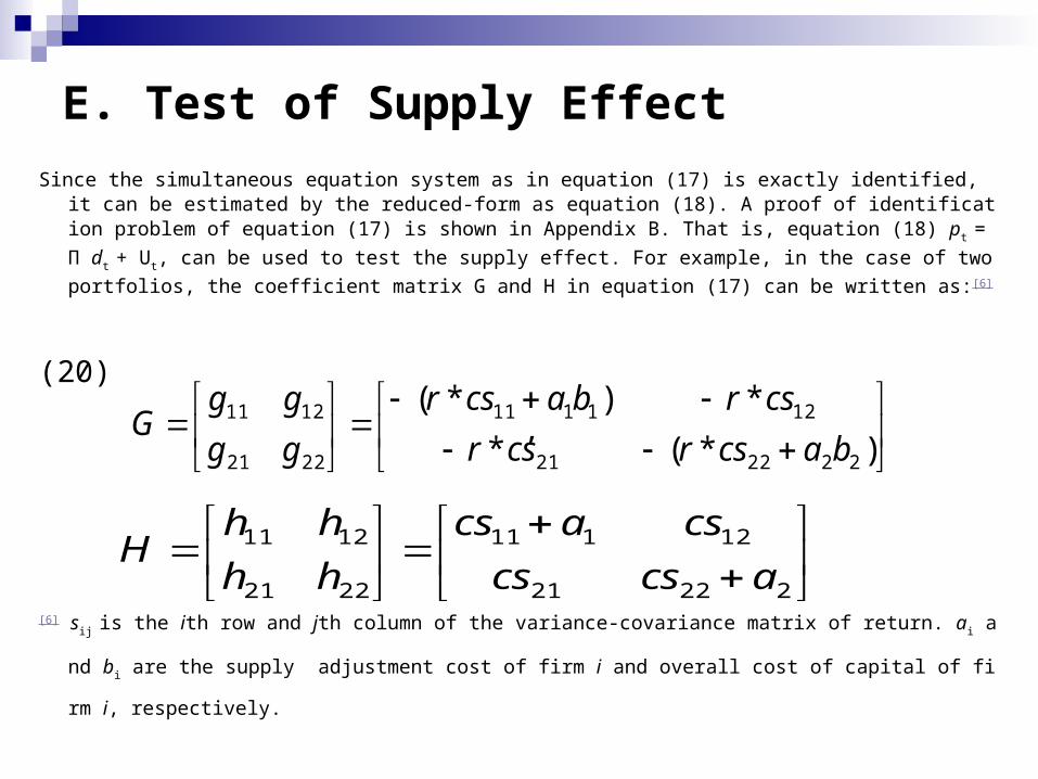
E. Test of Supply Effect Since the simultaneous equation system as in equation (17) is exactly identified, it can be es

timated by the reduced-form as equation (18). A proof of identification problem of equation (17) is shown in Appendix B. That is, equation (18) pt = Π dt + Ut, can be used to tes

t the supply effect. For example, in the case of two portfolios, the coefficient matrix G and H in equation (17) can be written as:[6]

(20) ,

[6] sij is the ith row and jth column of the variance-covariance matrix of return. ai and bi are t

he supply adjustment cost of firm i and overall cost of capital of firm i, respectively.

)*(*

*)*(

222221

121111

2221

1211

bacsrcsr

csrbacsr

gg

ggG

22221

12111

2221

1211

acscs

csacs

hh

hhH

E. Test of Supply Effect

Since Π = − G-1 H in equation (21), Π can be calculated as:

(21)

where

12221

12111

1

222221

1211111

**

**

acscs

csacs

bacsrcsr

csrbacsrHG

12221

12111

111121

122222

**

**1

acscs

csacs

bacsrcsr

csrbacsr

G

2221

1211

22 2 2 11 1 12 2111 ( * )( ) *r cs a b cs a r cs cs

22 2 2 12 12 22 112 ( * ) * ( )r cs a b cs r cs cs a

21 11 1 11 11 1 22 1* ( ) ( * )r cs cs a r cs a b cs

21 12 11 1 12 22 2 1* ( * )( )r cs cs r cs a b cs a

E. Test of Supply Effect From equation (21), if there is a high enough quadratic cost of adjustment,

or if a1 = a2 = 0, then with s12 = s21, the matrix would become a scalar matrix

in which diagonal elements are equal to r*c2 (s11 s22 − s122), and the off-

diagonal elements are all zero. In other words, if there is high enough cost of adjustment, firm tends to stop seeking to raise new funds or to retire old securities. Mathematically, this will be represented in a way that all off-diagonal elements are all zero and all diagonal elements are equal to each other in matrix П. In general, this can be extended into the case of more portfolios. For example, in the case of N portfolios, equation (18) becomes

(22)

Nt

t

t

Nt

t

t

NNNN

N

N

Nt

t

t

u

u

u

d

d

d

p

p

p

2

1

2

1

21

22221

11211

2

1

E. Test of Supply Effect Equation (22) shows that if an investor expects a change in the prediction of the

next dividend due to additional information (e.g., change in earnings) during the current period, then the price of the security changes. Regarding the international equity markets, if one believes that the global financial market is perfectly integrated (i.e., if one believes that how the expectation errors in dividends are built into the current price is the same for all securities), then the price changes would be only influenced by its own dividend expectation errors. Otherwise, say if the supply of securities is flexible, then the change in price would be influenced by the expectation adjustment in dividends of all other countries as well as that in its own country’s dividend.

Therefore, two hypotheses related to supply effect to be tested regarding the parameters in the reduced form system shown in equation (18):

Hypothesis 1: All the off-diagonal elements in the coefficient matrix Π are zero if the supply effect does not exist.

Hypothesis 2: All the diagonal elements in the coefficients matrix Π are equal in the magnitude if the supply effect does not exist.

E. Test of Supply Effect These two hypotheses should be satisfied jointly. That is, if the supply

effect does not exist, price changes of a security (index) should be a function of its own dividend expectation adjustments, and the coefficients should all be equal across securities. In the model described in equation (16), if an investor expects a change in the prediction of the next dividend due to the additional information during the current period, then the price of the security changes.

Under the assumption of the integration of the global financial market or the efficiency in the domestic stock market, if the supply of securities is fixed, then the expectation errors in dividends are built in the current price is the same for all securities. This phenomenon implies that the price changes would only be influenced by its own dividend expectation adjustments. If the supply of securities is flexible, then the change in price would be influenced by the expectation adjustment in dividends of all other securities as well as that of its own dividend.

III. DATA and EMPIRICAL RESULTS

A. International Equity Markets –Country Indices

1. Data and descriptive statistics 2. Dynamic CAPM with supply effect

B. United States Equity Markets – S&P500 1 Data and descriptive statistics 2 Dynamic CAPM with Supply Side Effect

III. DATA and EMPIRICAL RESULTS

In this section, we analyze two different types of markets--the international equity market and the U.S. domestic stock market. Most details of the model, the methodologies, and the hypotheses for empirical tests are previously discussed in Section II. However, before testing the hypotheses, some other details of the related tests that are needed to support the assumptions used in the model are also briefly discussed in this section. The first part of this section examines international asset pricing, and second part discusses the domestic asset pricing in the U.S. stock market.


We first examine the existence of supply effect in terms of the data of international equity markets. This set of data is used to explain why a dynamic CAPM may be a better choice in international asset pricing model.

1. Data and descriptive statistics The data come from two different sources. One is the Global Financial

Data from the databases of Rutgers Libraries, and the second set of dataset is the MSCI (Morgan Stanley Capital International, Inc.) equity indices. Most research of this paper uses the first dataset; however, MSCI indices are sometimes used for comparison. Both sets of data are used in performing Granger-causality test in this paper. The monthly dataset consists of the index, dividend yield, price earnings ratio, and capitalization for each equity market. Sixteen country indices and two world indices are used to do the empirical study, as presented in Table 1. For all country indices, dividends and earnings are all converted into U.S. dollar denominations. The exchange rate data also comes from Global Financial Data. These monthly series start from February 1988 to March 2004.


In Table 2, Panel A shows the first four moments of monthly returns and the Jarque-Berra statistics for testing normality for the two world indices and the seven indices of G7countries, and Panel B provides the same summary information for the indices of nine emerging markets. As can be seen in the mean and standard deviation of the monthly returns, the emerging markets tend to be more volatile than developed markets though they may yield opportunity of higher return. The average of monthly variance of return in emerging markets is 0.166, while the average of monthly variance of return in developed countries is 0.042.


2. Dynamic CAPM with supply effect

Recall from the previous section, the structural form equations are

exactly identified, and the series of expectation adjustments in d

ividend, dt, are exogenous variables. Now, the reduced form equ

ations can be used to test the supply effect. That is, equation (2

2) needs to be examined by the following hypotheses:

Hypothesis 1: All the off-diagonal elements in the coefficient matri

x Π are zero if the supply effect does not exist.

Hypothesis 2: All the diagonal elements in the coefficients matrix

Π are equal in the magnitude if the supply effect does not exist.


These two hypotheses should be satisfied jointly. That is, if the supply effect does not exist, price changes of each country’s index would be a function of its own dividend expectation adjustments, and the coefficients should be equal across all countries.

The estimated results of the simultaneous equations system are summarized in Table 3. The report here is from the estimates of seemingly unrelated regression (SUR) method.[7] Under the assumption that the global equity market consists of these sixteen counties, the estimations of diagonal elements vary across countries, and some of the off-diagonal elements are statistically significantly different from zero. The results from G7 and the emerging markets are also reported separately in Table 4 Panel A and B, respectively. The elements in these two matrices are similar to the elements in matrix П. However, simply observing the elements in matrix П directly can not justify or reject the null hypotheses derived for testing the supply effect. Two tests should be done separately to check whether these two hypotheses can be both satisfied.

[7] The estimates are similar to the results of full information maximum likelihood (FIML) method.


For the first hypothesis, the test of supply effect on off-diagonal elements, the foll

owing regression is run for each country:

pi, t = βi di, t + Σj≠i βj dj, t + εi, t, i, j = 1, …,16.

The null hypothesis then can be written as: H0: βj = 0, j=1, …, 16, j ≠i. The results

are reported in Table 5. Two test statistics are reported. The first test uses an F

distribution with 15 and 172 degrees of freedom, and the second test uses a ch

i-squared distribution with 15 degrees of freedom. Most countries have F-stati

stics and chi-squared statistics that are statistically significant; thus, the null hy

pothesis is rejected at different levels of significance in most countries.


For the second test, the following null hypothesis needs to be tested:

H0: πi,i = πj,j for all i, j=1, …, 16 Under the above fifteen restrictions, the Wald test statistic has a c

hi-square distribution with 15 degrees of freedom. The statistic is 165.03, which corresponds to a p-value of 0.000. One can reject the null hypothesis at any conventional levels of significance. In other words, the diagonal elements are obviously not equal to each other. From these two tests, the two hypotheses cannot be satisfied jointly, and the non-existence of the supply effect is rejected. Thus, the empirical results suggest the existence of supply effect in international equity markets.

B. United States Equity Markets – S&P500

This section examines the hypotheses derived earlier for the U.S. domestic stock market. Similar to the previous section, we test for the rejection of the existence of supply effect when market is assumed in equilibrium. If the supply of risky assets is responsive to its price, then large price changes which due to the change in expectation of future dividend, will be spread over time. In other words, there exists supply effect in the U.S. domestic stock markets. This implies that the dynamic instead of static CAPM should be used for testing capital assets pricing in the equity markets of United State.


1. Data and descriptive statisticsThree hundred companies are selected from the S&P500 and

grouped into ten portfolios with equal numbers of thirty companies by their payout ratios. The data are obtained from the COMTUSTAT North America industrial quarterly data. The data starts from the first quarter of 1981 to the last quarter of 2002. The companies selected satisfy the following two criteria. First, the company appears on the S&P500 at some time period during 1981 through 2002. Second, the company must have complete data available--including price, dividend, earnings per share and shares outstanding--during the 88 quarters (22 years). Firms are eliminated from the sample list if one of the following two conditions occurs.

(i) reported earnings are either trivial or negative,(ii) reported dividends are trivial.


Three hundred fourteen firms remain after these adjustments. Finally, excluding those seven companies with highest and lowest average payout ratio, the remaining 300 firms are grouped into ten portfolios by the payout ratio. Each portfolio contains 30 companies. Figure 1 shows the comparison of S&P500 index and the value-weighted index of the 300 firms selected (M). Figure 1 shows that the trend is similar to each other before the 3rd quarter of 1999. However, there exist some differences after 3rd quarter of 1999.

To group these 300 firms, the payout ratio for each firm in each year is determined by dividing the sum of four quarters’ dividends by the sum of four quarters’ earnings; then, the yearly ratios are further averaged over the 22-year period. The first 30 firms with highest payout ratio comprises portfolio one, and so on. Then, the value-weighted average of the price, dividend and earnings of each portfolio are computed. Characteristics and summary statistics of these 10 portfolios are presented in Table 6 and Table 7, respectively.


Table 7 shows the first four moments of quarterly returns of the market portfolio and ten portfolios. The coefficients of skewness, kurtosis, and Jarque-Berra statistics show that one can not reject the hypothesis that log return of most portfolios is normal. The kurtosis statistics for most sample portfolios are close to three, which indicates that heavy tails is not an issue. Additionally, Jarque-Berra coefficients illustrate that the hypotheses of Gaussian distribution for most portfolios are not rejected. It seems to be unnecessary to consider the problem of heteroskedasticity in estimating domestic stock market if the quarterly data are used.

B. United States Equity Markets – S&P5002. Dynamic CAPM with supply side effectIf one believes that the stock market is efficient (i.e., if one believes the way in

which the expectation errors in dividends are built in the current price is the same for all securities), then price changes would be influenced only by its own dividend expectation errors. Otherwise, if the supply of securities is flexible, then the change in price would be influenced by the expectation adjustment in dividends of other portfolios as well as that in its own dividend. Thus, two hypotheses related to supply effect are to be tested and should be satisfied jointly in order to examine whether there exists a supply effect.

The estimated coefficients of the simultaneous equations system for ten portfolios are summarized in Table 8.8 Results of Table 8 indicate that the estimated diagonal elements seem to vary across portfolios and most of the off-diagonal elements are significant from zero. Again, the null hypotheses can be tested by the tests mentioned in the previous section. The results of the test on off-diagonal elements (Hypothesis 1) are reported in Table 9 with the F-statistic. The null hypothesis is rejected at 5% level in six out of ten portfolios, but only two are rejected at 1% level. This result indicates that the null hypothesis can be rejected at 5% significant level.

8 The results are similar when using either the FIML or SUR approach. We report here is the estimates of SUR method.


For the second hypothesis, the following null hypothesis needs to be tested. H0: πi,i = πj,j for all i, j=1, …, 10. Under the above nine restriction, the Wald test statistic has a chi-square distribution with nine degrees of freedom. The statistic is 18.858, which is greater than 16.92 at 5% significance level. Since the statistic corresponds to a p-value of 0.0265, one can reject the null hypothesis at 5%, but it cannot reject H0 at a 1% significance level. In other words, the diagonal elements are not similar to each other in magnitude. In conclusion, the empirical results are sufficient to reject two null hypotheses of non-existence of supply effect in the U.S. stock market.

IV. SUMMARY AND CONCLUDING REMARKS

A. Summary

B. Future Research

A. SummaryWe examine an asset pricing model that incorporates a firm’s decision

concerning the supply of risky securities into the CAPM. This model focuses on a firm’s financing decision by explicitly introducing the firm’s supply of risky securities into the static CAPM and allows the supply of risky securities to be a function of security price. And thus, the expected returns are endogenously determined by both demand and supply decisions within the model. In other words, the supply effect may be one important factor in capital assets pricing decisions.

Our objectives are to investigate the existence of supply effect in both international equity markets and U.S. stock markets. The test results show that the two null hypotheses of the non-existence of supply effect do not seem to be satisfied jointly in both our data sets. In other words, this evidence seems to be sufficient to support the existence of supply effect, and thus, imply a violation of the assumption in the one period static CAPM, or imply a dynamic asset pricing model may be a better choice in both international equity markets and U.S. domestic stock markets.

B. Future ResearchApplication of Production Function in Finance and Accounting

Research By Cheng Few Lee, Shu-Hsing Li, and Bi-Huei Tsai

Outline A. IntroductionB. Basic concept and theory of production functionC. CAPM and production functionD. Application of production function in banking researchE. Application of production function in managerial researchF. Integration and extensionG. SummaryReferences

Table 1. World Indices and Country Indices List

I. World Indices

WI World index: FT-Actuaries World $ Index (w/GFD extension)

WIXUS World index excluding U.S.

Table 1. (Cont.)

II. Country IndicesAG Argentina: Buenos Aires SE General Index (IVBNG)

BZ Brazil: Brazil Bolsa de Valores de Sao Paulo (Bovespa) (_BVSPD)

CD Canada: Canada S&P/TSX 300 Composite Index (_GSPTSED)

FR France: Paris CAC-40 Index (_FCHID)

GM German: Germany Deutscher Aktienindex (DAX) (_GDAXD)

IT Italy: Banca Commerciale Italiana General Index (_BCIID)

HK Hong King: Hong Kong Hang Seng Composite Index (_HSID)

JP Japan: Japan Nikkei 225 Stock Average (_N225D)

MA Malaysia: Malaysia KLSE Composite (_KLSED)

MX Mexico: Mexico SE Indice de Precios y Cotizaciones (IPC) (_MXXD)

SG Singapore: Singapore Straits-Times Index (_STID)

KO South Korea: Korea SE Stock Price Index (KOSPI) (_KS11D)

TW Taiwan: Taiwan SE Capitalization Weighted Index (_TWIID)

TL Thailand: Thailand SET General Index (_SETID)

UK United Kingdom: UK Financial Times-SE 100 Index (_FTSED)

US United States: S&P 500 Composite (_SPXD)

Table 2: Summary Statistics of Monthly Return1, 2

Panel A: G7 and World Indices

Country Mean Std. Dev. Skewness Kurtosis Jarque-Bera

WI 0.0051 0.0425 -0.3499 3.3425 4.7547

WI excl.US 0.0032 0.0484 -0.1327 3.2027 0.8738

CD 0.0064 0.0510 -0.6210 4.7660 36.515**

FR 0.0083 0.0556 -0.1130 3.1032 0.4831

GM 0.0074 0.0645 -0.3523 4.9452 33.528**

IT 0.0054 0.0700 0.2333 3.1085 1.7985

JP -0.00036 0.0690 0.3745 3.5108 6.4386*

UK 0.0056 0.0474 0.2142 3.0592 1.4647

US 0.0083 0.0426 -0.3903 3.3795 5.9019

Table 2: Summary Statistics of Monthly Return1, 2

Panel B: Emerging Markets

Country Mean Std. Dev. Skewness Kurtosis Jarque-Bera

AG 0.0248 0.1762 1.9069 10.984 613.29**

BZ 0.0243 0.1716 0.4387 6.6138 108.33**

HK 0.0102 0.0819 0.0819 4.7521 26.490**

KO 0.0084 0.1210 1.2450 8.6968 302.79**

MA 0.0084 0.0969 0.5779 7.4591 166.22**

MX 0.0179 0.0979 -0.4652 4.0340 15.155**

SG 0.0072 0.0746 -0.0235 4.8485 26.784**

TW 0.0092 0.1192 0.4763 4.0947 16.495**

TL 0.0074 0.1223 0.2184 4.5271 19.763** Notes: 1 The monthly returns from Feb. 1988 to March 2004 for international markets.

2 * and ** denote statistical significance at the 5% and 1%, respectively.

Table 3: Coefficients for matrix П (all sixteen markets) P_CD P_FR P_GM P_IT P_JP P_UK P_US P_TW P_TH P_SG P_MX P_MA P_KO P_HK P_BZ P_AG

CD 0.416 0.626 0.750 0.232 0.608 0.233 0.282 0.130 0.066 1.003 1.130 0.126 0.035 3.080 0.564 1.221

[ 4.786] [ 4.570] [ 4.106] [ 4.210] [ 1.264] [ 2.460] [ 2.623] [ 1.376] [ 0.743] [ 2.583] [ 3.560] [ 2.056] [ 1.010] [ 2.935] [ 2.698] [ 3.114]

FR 0.003 0.038 0.015 -0.008 0.067 -0.015 0.001 -0.036 -0.027 -0.170 -0.144 -0.030 0.012 -0.067 -0.020 -0.110

[ 0.145] [ 1.121] [ 0.342] [-0.585] [ 0.567] [-0.650] [ 0.024] [-1.522] [-1.247] [-1.771] [-1.845] [-1.968] [ 1.347] [-0.260] [-0.390] [-1.137]

GM -15.03 40.376 43.677 8.090 -6.208 9.340 -28.52 -8.987 2.107 -79.09 -78.51 2.538 -4.437 -75.61 13.109 -54.23

[-0.771] [ 1.312] [ 1.064] [ 0.653] [-0.057] [ 0.439] [-1.181] [-0.423] [ 0.105] [-0.907] [-1.101] [ 0.184] [-0.566] [-0.321] [ 0.279] [-0.616]

IT 0.043 0.029 0.062 0.099 -0.030 0.022 0.014 0.000 0.014 0.155 0.275 -0.024 0.002 0.455 0.043 0.272

[ 0.980] [ 0.427] [ 0.683] [ 3.585] [-0.124] [ 0.473] [ 0.265] [-0.002] [ 0.321] [ 0.799] [ 1.730] [-0.789] [ 0.115] [ 0.867] [ 0.413] [ 1.390]

JP 0.058 0.087 0.073 0.020 0.801 0.069 0.083 0.035 0.012 0.173 0.203 -0.003 0.023 0.466 0.086 0.080

[ 3.842] [ 3.641] [ 2.300] [ 2.101] [ 9.537] [ 4.205] [ 4.396] [ 2.132] [ 0.746] [ 2.558] [ 3.668] [-0.242] [ 3.777] [ 2.546] [ 2.366] [ 1.173]

UK -22.313 29.783 13.186 -7.778 99.863 127.70 -23.812 -43.206 -14.772 28.205 -23.034 20.639 -15.315 -23.313 -58.263 -72.967

[-0.897] [ 0.759] [ 0.252] [-0.492] [ 0.724] [ 4.707] [-0.773] [-1.595] [-0.578] [ 0.254] [-2.533] [ 1.176] [-1.532] [-0.776] [-0.974] [-0.649]

US -29.480 -54.442 -56.122 -17.049 -61.119 -29.977 -23.036 -22.029 35.898 -80.345 -74.468 -25.152 -0.222 -18.695 -22.574 -82.626

[-2.287] [-2.717] [-2.100] [-2.114] [-0.868] [-2.165] [-1.464] [-0.159] [ 0.275] [-1.415] [-1.604] [-0.281] [-0.004] [-1.218] [-0.739] [-1.441]

TW -0.041 0.000 0.026 0.028 -0.070 -0.008 -0.038 0.030 -0.068 -0.280 -0.080 0.017 -0.030 -0.957 0.105 -0.407

[-0.634] [-0.004] [ 0.188] [ 0.684] [-0.194] [-0.120] [-0.479] [ 0.426] [-1.025] [-0.965] [-0.338] [ 0.361] [-1.138] [-1.222] [ 0.677] [-1.390]

TH -0.026 -0.050 -0.020 -0.035 0.021 -0.056 -0.068 0.017 0.031 0.099 -0.176 0.074 -0.001 -0.011 -0.022 -0.190

[-0.820] [-0.987] [-0.295] [-1.722] [ 0.117] [-1.608] [-1.727] [ 0.494] [ 0.943] [ 0.692] [-1.508] [ 3.280] [-0.059] [-0.028] [-0.284] [-1.315]

SG 0.025 0.039 0.017 0.008 0.028 0.031 0.039 0.029 0.023 0.222 0.050 0.018 0.008 0.479 0.048 0.078

[ 1.613] [ 1.623] [ 0.516] [ 0.854] [ 0.334] [ 1.867] [ 2.082] [ 1.737] [ 1.465] [ 3.264] [ 0.906] [ 1.666] [ 1.257] [ 2.606] [ 1.325] [ 1.134]

MX 0.011 0.024 0.034 0.003 -0.037 0.017 0.022 0.011 0.012 0.085 0.184 0.002 0.006 0.286 0.053 0.080

[ 1.189] [ 1.644] [ 1.736] [ 0.423] [-0.705] [ 1.672] [ 1.887] [ 1.033] [ 1.212] [ 2.018] [ 5.341] [ 0.248] [ 1.492] [ 2.518] [ 2.323] [ 1.886]

MA 0.019 -0.110 -0.064 -0.026 0.304 0.048 -0.019 -0.073 0.011 0.018 -0.060 0.057 0.009 -0.160 -0.160 -0.344

[ 0.276] [-0.992] [-0.431] [-0.590] [ 0.780] [ 0.628] [-0.224] [-0.958] [ 0.150] [ 0.059] [-0.234] [ 1.160] [ 0.333] [-0.189] [-0.947] [-1.085]

KO 0.103 0.071 -0.077 0.037 1.007 0.070 0.176 -0.005 0.029 0.449 0.077 -0.045 0.158 -0.726 -0.071 0.102

[ 1.262] [ 0.548] [-0.446] [ 0.706] [ 2.225] [ 0.782] [ 1.740] [-0.060] [ 0.345] [ 1.230] [ 0.257] [-0.789] [ 4.818] [-0.736] [-0.362] [ 0.278]

HK -0.012 -0.013 -0.008 -0.006 -0.013 -0.007 -0.009 0.003 -0.001 -0.021 -0.006 -0.001 -0.002 -0.006 -0.012 -0.008

[-2.844] [-1.921] [-0.891] [-2.158] [-0.540] [-1.549] [-1.736] [ 0.568] [-0.113] [-1.083] [-0.359] [-0.331] [-1.209] [-0.112] [-1.123] [-0.386]

BZ 0.009 0.017 0.023 0.005 -0.012 0.012 0.016 0.008 -0.003 0.012 0.050 0.004 0.000 0.017 0.053 0.060

[ 1.878] [ 2.337] [ 2.424] [ 1.855] [-0.490] [ 2.328] [ 2.907] [ 1.568] [-0.557] [ 0.605] [ 2.989] [ 1.226] [-0.068] [ 0.306] [ 4.801] [ 2.902]

AG 0.007 0.008 0.008 0.001 -0.001 0.008 0.008 0.001 0.005 0.000 0.049 0.002 0.000 0.061 0.009 0.094

[ 1.466] [ 1.056] [ 0.857] [ 0.356] [-0.025] [ 1.614] [ 1.326] [ 0.255] [ 1.012] [-0.004] [ 2.879] [ 0.604] [-0.017] [ 1.081] [ 0.776] [ 4.464]

R 0.3148 0.31 0.2111 0.2741 0.4313 0.3406 0.2775 0.1241 0.0701 0.2148 0.3767 0.1479 0.2679 0.1888 0.2435 0.2639

F 5.2676 5.151 3.0692 4.3299 8.6948 5.9235 4.4049 1.6245 0.8642 3.1376 6.9313 1.9898 4.196 2.6688 3.69 4.1112

Table 4 Table 4: Coefficients for matrix П

Panel A: G7 countries*

CD FR GM IT JP UK US

Canada (CD) 0.4285 0.6293 0.7653 0.2302 0.5960 0.2415 0.2877 [ 4.83222] [ 4.53805] [ 4.21660] [ 4.16284] [ 1.26211] [ 2.50434] [ 2.58267]

France (FR) 0.0092 0.0479 0.0224 -0.0069 0.0659 -0.0132 0.0037 [ 0.43450] [ 1.45043] [ 0.51768] [-0.52404] [ 0.58564] [-0.57310] [ 0.14092]

German (GM) -22.2372 27.6389 29.0424 5.7762 -17.3229 1.3207 -42.1272 [-1.12604] [ 0.89492] [ 0.71849] [ 0.46895] [-0.16472] [ 0.06149] [-1.69824]

Italy (IT) 0.0522 0.0371 0.0799 0.1043 0.0342 0.0318 0.0330 [ 1.20922] [ 0.54894] [ 0.90383] [ 3.87215] [ 0.14853] [ 0.67670] [ 0.60883]

Japan (JP) 0.0738 0.1040 0.0864 0.0245 0.8312 0.0836 0.0996 [ 4.93698] [ 4.45014] [ 2.82459] [ 2.63259] [ 10.4454] [ 5.14208] [ 5.30466]

U. K. (UK) -40.7615 -0.8139 -16.2433 -16.6896 112.3044 112.3671 -44.9229 [-1.64160] [-0.02096] [-0.31960] [-1.07766] [ 0.84931] [ 4.16109] [-1.44029]

U. S. (US) -31.2190 -56.8336 -57.4718 -15.7037 -71.5680 -30.7517 -26.3700

[-2.42947] [-2.82807] [-2.18506] [-1.95935] [-1.04583] [-2.20045] [-1.63368]

R-squared 0.2294 0.2373 0.1605 0.2122 0.4095 0.2622 0.1641

F-statistic 8.9794 9.3872 5.7685 8.1274 20.9187 10.7183 5.9233

Note: *Numbers in [ ] are the t-value.

Table 4 Table 4: Coefficients for matrix П.

Panel B: Nine emerging markets*

TW TH SG MX MA KO HK BZ AG Taiwan 0.0279 -0.0686 -0.3535 -0.1396 0.0040 -0.0258 -1.1395 0.0761 -0.5048 (TW) [ 0.39388] [-1.05234] [-1.20100] [-0.54785] [ 0.08857] [-0.97462] [-1.43238] [ 0.48390] [-1.70195] Thailand 0.0167 0.0263 0.1122 -0.1344 0.0660 0.0068 0.1445 0.0008 -0.1593 (TH) [ 0.48456] [ 0.83246] [ 0.78605] [-1.08725] [ 2.99283] [ 0.53054] [ 0.37457] [ 0.01022] [-1.10720] Singapore 0.0315 0.0215 0.2163 0.0524 0.0142 0.0120 0.4915 0.0519 0.0574 (SG) [ 1.93909] [ 1.44098] [ 3.20829] [ 0.89816] [ 1.36499] [ 1.98318] [ 2.69713] [ 1.43966] [ 0.84543] Mexico 0.0133 0.0129 0.0923 0.1955 0.0025 0.0049 0.2794 0.0503 0.0864 (MX) [ 1.30151] [ 1.37317] [ 2.17164] [ 5.31170] [ 0.37451] [ 1.26819] [ 2.43220] [ 2.21608] [ 2.01656] Malaysia -0.0668 0.0227 0.1107 -0.0168 0.0664 0.0106 -0.0391 -0.1358 -0.3029 (MA) [-0.87856] [ 0.32527] [ 0.35080] [-0.06150] [ 1.36417] [ 0.37456] [-0.04584] [-0.80543] [-0.95281] S. Korea 0.0040 0.0302 0.5954 0.2211 -0.0516 0.1724 -0.3149 -0.0105 0.2073 (KO) [ 0.04516] [ 0.36871] [ 1.61091] [ 0.69078] [-0.90507] [ 5.17701] [-0.31514] [-0.05290] [ 0.55646] HongKong 0.0008 -0.0011 -0.0262 -0.0176 -0.0003 -0.0033 -0.0287 -0.0161 -0.0124 (HK) [ 0.16463] [-0.25388] [-1.33665] [-1.03852] [-0.10295] [-1.88424] [-0.54139] [-1.53139] [-0.62961] Brazil 0.0091 -0.0020 0.0176 0.0621 0.0034 0.0005 0.0380 0.0558 0.0686 (BZ) [ 1.84521] [-0.43841] [ 0.85699] [ 3.50359] [ 1.08063] [ 0.28347] [ 0.68631] [ 5.09912] [ 3.32283] Argentina 0.0026 0.0050 0.0092 0.0585 0.0024 0.0012 0.0950 0.0154 0.1004 (AG) [ 0.51493] [ 1.08871] [ 0.44123] [ 3.23312] [ 0.74046] [ 0.65121] [ 1.68184] [ 1.37500] [ 4.76894] R-squared 0.057384 0.050263 0.137001 0.231799 0.104100 0.191448 0.108119 0.179049 0.194793 F-statistic 1.362139 1.184153 3.552016 6.751474 2.599893 5.297943 2.712414 4.879985 5.412899 Note: *Numbers in [ ] are the t-value.

Table 5: Test of Supply Effect on off-Diagonal Elements of Matrix П1, 2 R 2 F- statistic p-value Chi-square p-value

Canada 0.3147 3.5055 0.0000 52.5819 0.0000

France 0.3099 4.6845 0.0000 70.2686 0.0000

German 0.2111 2.8549 0.0005 42.8236 0.0002

Italy 0.2741 2.9733 0.0003 44.6004 0.0001

Japan 0.4313 0.7193 0.7628 10.7894 0.7674

U.K. 0.3406 3.9361 0.0000 59.0413 0.0000

U.S. 0.2775 4.5400 0.0000 68.1001 0.0000

Taiwan 0.1241 1.6266 0.0711 24.3984 0.0586

Thailand 0.0701 0.7411 0.7401 11.1171 0.7442

Singapore 0.2148 2.1309 0.0106 31.9634 0.0065

Mexico 0.3767 4.7873 0.0000 71.8099 0.0000

Malaysia 0.1479 1.6984 0.0550 25.4755 0.0439

S. Korea 0.2679 2.1020 0.0118 31.5305 0.0075

Hongkong 0.1888 2.6836 0.0011 40.2540 0.0004

Brazil 0.2435 1.9174 0.0244 28.7613 0.0173

Argentina 0.2639 2.6210 0.0014 39.3155 0.0006

Notes: 1 pi, t = βi’di, t + Σj≠i βj’dj, t + ε’i, t, i, j = 1, …,16. Null Hypothesis: all βj = 0, j=1,…, 16, j ≠i

2 The first test uses an F di

stribution with 15 and 172 degrees of freedom, and the second test uses a chi-squared distribution with 15 degrees of freedom.

Table 6: Characteristics of Ten Portfolios

Notes: 1 The first 30 firms with highest payout ratio comprises portfolio one, and so on.2 The price, dividend and earnings of each portfolio are computed by value-weighted of the

30 firms included in the same category.3 The payout ratio for each firm in each year is found by dividing the sum of four quarters’

dividends by the sum of four quarters’ earnings, then, the yearly ratios are then computed from the quarterly data over the 22-year period.

Portfolio1 Return2 Payout3 Size (000) Beta (M)

1 0.0351 0.7831 193,051 0.7028

2 0.0316 0.7372 358,168 0.8878

3 0.0381 0.5700 332,240 0.8776

4 0.0343 0.5522 141,496 1.0541

5 0.0410 0.5025 475,874 1.1481

6 0.0362 0.4578 267,429 1.0545

7 0.0431 0.3944 196,265 1.1850

8 0.0336 0.3593 243,459 1.0092

9 0.0382 0.2907 211,769 0.9487

10 0.0454 0.1381 284,600 1.1007

Table 7: Summary Statistics of Portfolio Quarterly Returns1

Notes: 1 Quarterly returns from 1981:Q1 to 2002:Q4 are calculated.

2 * and ** denote statistical significance at the 5% and 1%, respectively.

CountryMean (quarterly

)

Std. Dev. (quarterly

)Skewness Kurtosis Jarque-Bera2

Marketportfolio

0.0364 0.0710 -0.4604 3.9742 6.5142*

Portfolio 1 0.0351 0.0683 -0.5612 3.8010 6.8925*

Portfolio 2 0.0316 0.0766 -1.1123 5.5480 41.470**

Portfolio 3 0.0381 0.0768 -0.3302 2.8459 1.6672*

Portfolio 4 0.0343 0.0853 -0.1320 3.3064 0.5928

Portfolio 5. 0.0410 0.0876 -0.4370 3.8062 5.1251

Portfolio 6. 0.0362 0.0837 -0.2638 3.6861 2.7153

Portfolio 7 0.0431 0.0919 -0.1902 3.3274 0.9132

Portfolio 8 0.0336 0.0906 0.2798 3.3290 1.5276

Portfolio 9 0.0382 0.0791 -0.2949 3.8571 3.9236

Portfolio 10 0.0454 0.0985 -0.0154 2.8371 0.0996

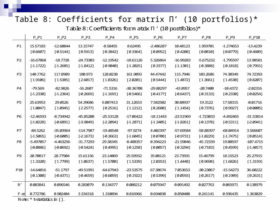
Table 8: Coefficients for matrix П’ (10 portfolios)* Table 8: Coefficients for matrix П’ (10 portfolios)*

P_P1 P_P2 P_P3 P_P4 P_P5 P_P6 P_P7 P_P8 P_P9 P_P10

P1 15.57183 -12.60844 13.15747 -8.58455 8.62495 -2.486287 10.48123 1.959701 -1.274653 -13.4239

[ 0.6607] [-0.5144] [ 0.5913] [-0.3842] [ 0.3364] [-0.0952] [ 0.4208] [ 0.0810] [-0.0779] [-0.4609]

P2 -16.67868 -18.7728 -24.73303 -12.19542 -18.61126 5.326864 -16.99283 -5.675232 -1.795597 13.98581

[-1.1722] [-1.2685] [-1.8412] [-0.9040] [-1.2025] [ 0.3377] [-1.1301] [-0.3888] [-0.1818] [ 0.7955] .

P3 140.7762 117.8989 180.973 128.0238 161.9093 44.47442 115.7946 103.2686 74.30349 74.72393

[ 1.9106] [ 1.5385] [ 2.6017] [ 1.8326] [ 2.0201] [ 0.5444] [ 1.4872] [ 1.3661] [ 1.4530] [ 0.8207]

P4 -79.569 -82.9826 -16.2607 -71.5316 -38.36708 -29.88297 -43.8957 -20.7400 -10.4372 -2.02316

[-1.2330] [-1.2364] [-0.2669] [-1.1691] [-0.5466] [-0.4177] [-0.6437] [-0.3133] [-0.2330] [-0.0254]

P5 25.63953 29.0526 54.39686 6.087413 31.12653 7.582502 30.88937 19.3122 17.58315 -0.01716

[ 1.0047] [ 1.0945] [ 2.2577] [ 0.2516] [ 1.1212] [ 0.2680] [ 1.1454] [ 0.7376] [ 0.9927] [-0.0005]

P6 -12.46593 -8.734942 -45.85208 -25.53128 -17.06422 -18.11443 -23.51969 -1.723033 -4.492465 -31.53814

[-1.0228] [-0.6891] [-3.9849] [-2.2094] [-1.2871] [-1.3405] [-1.8261] [-0.1378] [-0.5311] [-2.0941]

P7 -84.5262 -35.03964 -114.7987 -19.48548 -97.9274 4.402397 -57.69584 -58.88397 -68.04914 3.566607

[-1.5065] [-0.6005] [-2.1673] [-0.3663] [-1.6045] [ 0.0708] [-0.9731] [-1.0229] [-1.7475] [ 0.0514]

P8 -5.497057 -4.463256 -31.77293 29.38345 -8.488357 0.394223 -21.59846 -45.72339 19.80597 -107.4715

[-0.0886] [-0.0692] [-0.5424] [ 0.4995] [-0.1258] [ 0.0057] [-0.3294] [-0.7183] [ 0.4599] [-1.4017]

P9 20.70817 28.77904 15.61156 23.14069 25.93932 35.08121 23.73591 15.46799 18.15523 25.27915

[ 1.3320] [ 1.7799] [ 1.0637] [ 1.5700] [ 1.5339] [ 2.0353] [ 1.4448] [ 0.9698] [ 1.6826] [ 1.3159]

P10 -14.64016 -51.1797 -49.51991 -64.67943 -23.53575 67.38674 7.053653 -30.23067 -15.54273 36.60222

[-0.1300] [-0.4371] [-0.4659] [-0.6059] [-0.1922] [ 0.5399] [ 0.0593] [-0.2617] [-0.1989] [ 0.2631]

R2 0.083841 0.096546 0.283079 0.134377 0.088212 0.075947 0.091492 0.027763 0.065971 0.138979

F-st 0.772786 0.902404 3.334318 1.310894 0.816966 0.694038 0.850408 0.241141 0.596435 1.363029

Note: * t-statistics in [ ].

Table 9: Test of Supply Effect on off-Diagonal Elements of Matrix П1, 2, 3

Notes: 1 pi, t = βi’di, t + Σj≠i βj’dj, t + ε’i, t, i, j = 1, …,10.

Hypothesis: all βj = 0, j=1,…, 10, j ≠i

2 The first test uses an F distribution with 9 and 76 degrees of freedom, and the second uses a chi-squared distribution with 9 degrees of freedom.

3 * and ** denote statistical significance at the 5 and 1 percent level, respectively.

R 2 F- statistic p-value Chi-square p-value

Portfolio 1 0.1518 1.7392* 0.0872 17.392 0.0661

Portfolio 2 0.1308 1.4261 0.1852 14.261 0.1614

Portfolio 3 0.4095 5.4896** 0.0000 53.896 0.0000

Portfolio 4 0.1535 1.9240* 0.0607 17.316 0.0440

Portfolio 5 0.1706 1.9511* 0.0509 19.511 0.0342

Portfolio 6 0.2009 1.2094 0.2988 12.094 0.2788

Portfolio 7 0.2021 1.8161* 0.0718 18.161 0.0523

Portfolio 8 0.1849 1.9599* 0.0497 19.599 0.0333

Portfolio 9 0.1561 1.8730* 0.0622 18.730 0.0438

Portfolio 10 0.3041 3.5331** 0.0007 35.331 0.0001

Figure 1Comparison of S&P500 and Market portfolio

0

200

400

600

800

1000

1200

1400

1600

S&P500

M

Appendix A Modeling the Price Process

In Section II C, equation (16) is derived from equation (15) under the assumption that all countri

es’ index series follow a random walk process. Thus, before further discussion, we should te

st the order of integration of these price series. Two widely used unit root tests are the Dicke

y-Fuller (DF) and the augmented Dickey-Fuller (ADF) tests. The former can be represented

as:

Pt = μ + γ Pt-1 + εt, and the latter can be written as:

∆Pt = μ + γ Pt-1 + δ1 ∆Pt-1 + δ2 ∆Pt-2 +…+δp ∆Pt-p + εt.

The results of the tests for each index are summarized in Table A.1 It seems that one cannot

reject the hypothesis that the index follows a random walk process. In the ADF test the null

hypothesis of unit root in level can not be rejected for all indices whereas the null hypothesis of

unit root in the first difference is rejected. This result is consistent with most which conclude that

the financial price series follow a random walk process.

Appendix A Modeling the Price Process

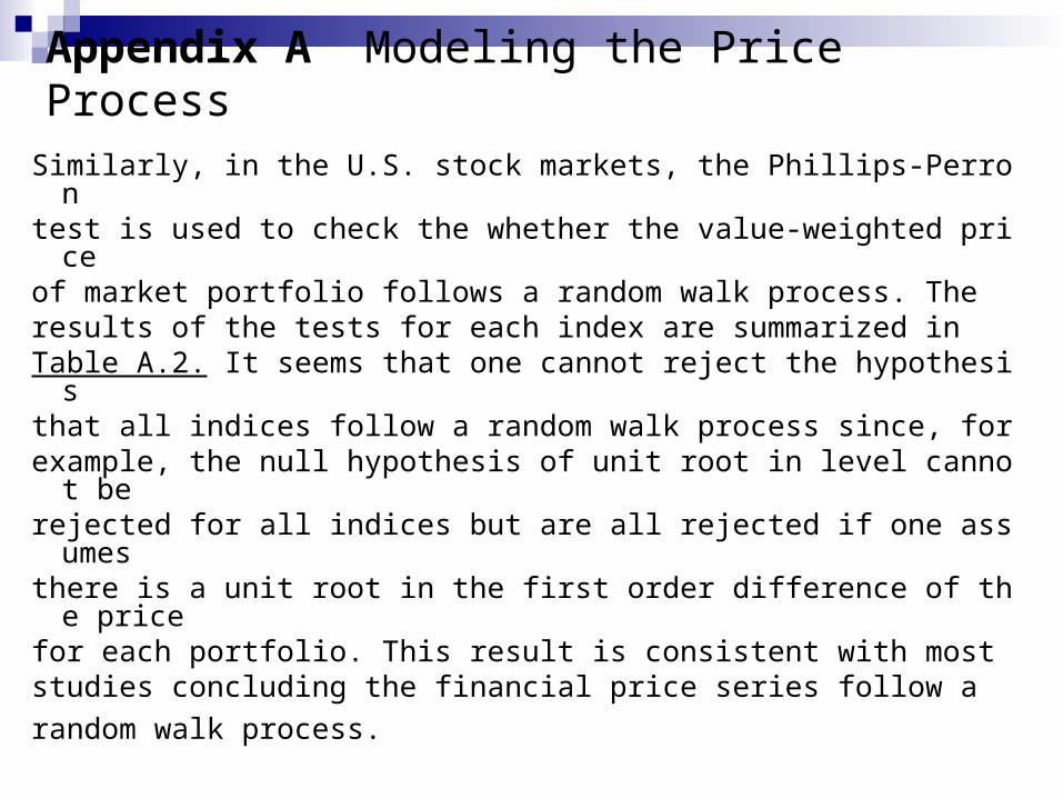
Similarly, in the U.S. stock markets, the Phillips-Perron test is used to check the whether the value-weighted price of market portfolio follows a random walk process. The results of the tests for each index are summarized in Table A.2. It seems that one cannot reject the hypothesis that all indices follow a random walk process since, for example, the null hypothesis of unit root in level cannot be rejected for all indices but are all rejected if one assumes there is a unit root in the first order difference of the price for each portfolio. This result is consistent with most studies concluding the financial price series follow a

random walk process.

Table A.1. Unit root tests for Pt

Pt = μ + γ Pt-1 + εt Unit root test (ADF)

Estimated c2

(Std. Error)R2 Level 1st Difference

World Index 0.9884 (0.0098), 0.9820 0.63 -13.74**

W.I. ex. U.S. 0.9688 (0.0174) 0.9434 0.13 -14.03**

Argentina 0.9643 (0.0177) 0.9411 -0.70 -13.08**

Brazil 0.9738 (0.0160) 0.9520 -0.65 -12.49**

Canada 0.9816 (0.0156) 0.9550 -0.69 -11.80**

France 0.9815 (0.0121) 0.9725 0.34 -14.06**

Germany 0.9829 (0.0119) 0.9736 0.12 -14.53**

Hong Kong 0.9754 (0.0146) 0.9599 -1.68 -13.87**

Table A.1. (Cont.)

Note: ** 1% significant level

Pt = μ + γ Pt-1 + εt Unit root test (ADF)

Estimated c2

(Std. Error)R2 Level 1st Difference

Italy 0.9824 (0.0136) 0.9656 0.24 -15.42**

Japan 0.9711 (0.0185) 0.9368 -1.02 -14.32**

Malaysia 0.9757 (0.0145) 0.9603 -0.64 -7.01**

Mexico 0.9749 (0.0159) 0.9531 -0.26 -13.39**

Singapore 0.9625 (0.0173) 0.9432 0.02 -14.08**

S. Korea 0.9735 (0.0170) 0.9463 -0.67 -12.61**

Taiwan 0.9295 (0.0263) 0.8706 -0.54 -12.49**

Thailand 0.9854 (0.0124) 0.9715 -0.49 -12.79**

U.K. 0.9875 (0.0094) 0.9835 0.53 -13.76**

U.S. 0.9925 (0.0076) 0.9892 0.82 -14.10**

Table A.2. Unit root tests for Pt

Notes: 1* 5% significant level; ** 1% significant level 2 The process assumed to be random walk without drift. 3 The null hypothesis of zero intercept terms, μ, can not be rejected at 5%, 1% level for all portfolios.

Pt = μ + γ Pt-1 + εt Phillips-Perron test1, 2

Estimated c2

(Std. Error)Adj. R2 Level 1st Difference3

Market portfolio 1.0060 (0.0159) 0.9788 -0.52 -8.48**

S&P500 0.9864 (0.0164) 0.9769 -0.90 -959**

Portfolio 1 0.9883 (0.0172) 0.9746 -0.56 -8.67**

Portfolio 2 0.9877 (0.0146) 0.9815 -0.97 -9.42**

Portfolio 3 0.9913 (0.0149) 0.9809 -0.51 -13.90**

Portfolio 4 0.9935 (0.0143) 0.9825 -0.61 -7.66**

Portfolio 5 0.9933 (0.0158) 0.9787 -0.43 -9.34**

Portfolio 6 0.9950 (0.0150) 0.9808 -0.32 -8.66**

Portfolio 7 0.9892 (0.0155) 0.9793 -0.64 -9.08**

Portfolio 8 0.9879 (0.0166) 0.9762 -0.74 -9.37**

Portfolio 9 0.9939 (0.0116) 0.9884 -0.74 -7.04**

Portfolio 10 0.9889 (0.0182) 0.9716 -0.69 -9.07**

APPENDIX A. MODELING THE PRICE PROCESS

In Section II.C, equation (16) is derived from equation (15) under the assumption that all countries’ index series follow a random walk process. Thus, before further discussion, we should test the order of integration of these price series. Two widely used unit root tests are the Dickey-Fuller (DF) and the augmented Dickey-Fuller (ADF) tests. The former can be represented as: Pt = μ + γ Pt-1 + εt, and the latter can be written as: ∆Pt = μ + γ Pt-1 + δ1 ∆Pt-1 + δ2 ∆Pt-2 +…+δp ∆Pt-p + εt. The results of the tests for each index are summarized in Table A.1 It seems that one cannot reject the hypothesis that the index follows a random walk process. In the ADF test, the null hypothesis of unit root in level can not be rejected for all indices whereas the null hypothesis of unit root in the first difference is rejected. This result is consistent with most studies that conclude that the financial price series follow a random walk process.

APPENDIX A. MODELING THE PRICE PROCESS

Similarly, in the U.S. stock markets, the Phillips-Perron test is used to check the whether the value-weighted price of market portfolio follows a random walk process. The results of the tests for each index are summarized in Table A.2. It seems that one cannot reject the hypothesis that all indices follow a random walk process since, for example, the null hypothesis of unit root in level cannot be rejected for all indices but are all rejected if one assumes there is a unit root in the first order difference of the price for each portfolio. This result is consistent with most studies that find that the financial price series follow a random walk process.

Appendix B.

Identification of the Simultaneous Equation System

g11 g12 …… g1n h11 h12 …… h1n

g21 g22 …… g1n h21 h22 …… h2n

. . . . gn1 gn2 …… gnn hn1 hn2 …… hnn

where A = [G H] =

π11 π12 …… π1n 1 0 …… 0 ’ π21 π22 …… π1n 0 1 …… 0 . . . . πn1 πn2 …… πnn 0 0 …… 1

W = [Π I n]’ =

Note that given G is nonsingular, Π = −G-1 H in equation (19) can be written as

(B-1) AW = 0

Appendix B. Identification of the Simultaneous Equation System

That is, A is the matrix of all structure coefficients in the model with dimension of (n × 2n) and W is a (2n × n) matrix. The first equation in (A.1) can be expressed as

(B-2) A1W = 0,

where A1 is the first row of A, i.e.,

A1= [g11 g12….g1n h11 h12…..h1n].


Since the elements of Π can be consistently estimated, and In is the identity matrix, equation (B-2) contains 2n unknowns in terms of π’s. Thus, there should be n restrictions on the parameters to solve equation (B-2) uniquely. First, one can try to impose normalization rule by setting g11 equal to 1 to reduce one restriction. As a result, there are at least n-1 independent restrictions needed in order to solve (B-2).

It can be illustrated that the system represented by equation (17) is exactly identified with three endogenous and three exogenous variables. It is entirely similar to those cases of more variables. For example, if n=3, equation (17) can be expressed in the form


(B-3)

p1t

p2t

p3t

r*cs11 + a1 b1 r*cs12 r*cs13

r*cs21 r*cs22 + a2 b2 r*cs23

r*cs31 r*cs32 r*cs33 + a3 b3

─

d1t d2t

d3t

cs11 + a1 cs12 cs13

cs21 cs22 + a2 cs23

cs31 cs32 cs33 + a3

v1t v2t

v3t

+

=

Where r* = scalar of riskfree rate

sij = elements of variance-covariance matrix of return,

ai = inverse of the supply adjustment cost of firm i,

bi = overall cost of capital of firm i.


p1t p2t

p3t

g11 g12 g13

g21 g22 g23

g31 g32 g33

─ d1t d2t

d3t

h11 h12 h13

h21 h22 h23

h31 h32 h33

v1t v2t

v3t

+

=

(B-4)

(B-5) Φ = 0 1 0 0 r* 00 0 1 0 0 r*

’

For Example, in the case of n=3, equation (17) can be written as

Comparing (B-3) with (B-4), the prior restrictions on the first equation take the form, g12= -r*h12 and g13= -r*h13, and so on.

Thus, the restriction matrix for the first equation is of the form:


Then, combining (B-2) and the parameters of the first equation gives

π11 π12 π13 0 0

π21 π22 π13 1 0 π31 π32 π33 0 1

1 0 0 0 0

0 1 0 r* 0

0 0 1 0 r*

(B-6) [g11 g12 g13 h11 h12 h13] = [0 0 0 0 0 0]


That is, extending (B-6), we have

g11 π11 + g12 π21 + g13π31 + h11 = 0,

g11 π12 + g12 π22 + g13π32 + h12 = 0,

(B-7) g11 π13 + g12 π23 + g13π33 + h13 = 0,

g12 + r* h12 = 0, and

g13 + r* h13 = 0.


The last two (n-1 = 3-1 = 2) equations in (B-7) give the value h12 and h13 and the normalization condition, g11 = 1,

allow us to solve equation (B-2) in terms of π’s uniquely. That is, in the case n=3, the first equation represented by (B-2), A1W = 0, can be finally rewritten as (B-7). Sinc

e there are three unknowns, g12, g13 and h11, left for the fi

rst three equations in (B-7), the first equation A1 is exact

ly identified. Similarly, it can be shown that the second and the third equations are also exactly identified.

A Dynamic CAPM with Supply Effect: Theory and Empirical Results Dr. Cheng Few Lee Distinguished...

Documents

Transcript of A Dynamic CAPM with Supply Effect: Theory and Empirical Results Dr. Cheng Few Lee Distinguished...