A Dwindling Role for Coal - Union of Concerned … Dwindling Role for Coal | 1 This document details...

A Dwindling Role for Coal Tracking the Electricity Sector

Transition and What It Means for

the Nationwww.ucsusa.org/coaltransition

Appendix: Technical Document

© October 2017

All rights reserved

http://sharepoint.ucsusa.org/programs/ce/ProjectsandCampaigns/Power%20Ahead/Analytics/Clean%20Energy%20Transition%20Analysis%20FY17/Release%20Materials/www.ucsusa.org/coaltransition

A Dwindling Role for Coal | 1

This document details the methods and data used in the Clean Energy Transition analysis by the Union of Concerned Scientists

(UCS). The full suite of materials, including a fact sheet, community snapshots, and interactive maps, can be found online at

www.ucsusa.org/coaltransition.

The analysis is rooted in the work of two prior UCS reports: Ripe for Retirement: The Case for Closing America’s

Costliest Coal Plants (Cleetus et al. 2012) and Ripe for Retirement: An Economic Analysis of the US Coal Fleet (Fleischman et al.

2013). As in the previous analyses, this study assesses the economic competitiveness of the current coal fleet by comparing the

operating costs of today’s coal generators to those of other energy resources. By combining the resulting findings with public data

on planned future retirements, the analysis illuminates the potential scale and scope of the fleet’s transition over the coming years.

In addition to looking forward, however, this iteration of the analysis also looks back. In recognition of the fact that the US

power sector has quickened its retreat from coal even since the 2012 and 2013 UCS reports, this analysis also characterizes and

quantifies the extent of the coal fleet evolution between 2008 and 2016, providing past context for the future transition.

Finally, this work also expands on the previous analyses by including a proximity analysis that considers how the

transition at the fleet level has been reflected in communities living close to coal generators across the country—and how it could be

reflected as the transition continues. Following methodologies established by the Environmental Protection Agency (EPA), the

project includes a proximity analysis for all coal units operating in 2008, identifying the total population, as well as the minority and

low-income populations, living within a three-mile radius of individual coal units. From there, the analysis considers whether and

when coal units located in these communities retired or converted to a different fuel, as well as whether and which additional units

in these communities may be uneconomic. This analysis follows methods established by the EPA for its EJ Screening Report for the

Clean Power Plan (EPA 2015), and additionally used in its EJSCREEN Tool, as found online at www.epa.gov/ejscreen.

This document contains a section on methodology and assumptions followed by a section describing detailed results and

findings. The first section includes an explanation of the methodology and assumptions for (1) identifying and characterizing the

coal units operating—and retiring or converting—in 2008, 2016, and the near future; (2) calculating the operating costs used to

identify uneconomic coal units; (3) assessing the costs of alternative resources used to conduct the economic stress test, as well as

sensitivities, the presence of pollution control technologies, and limitations of the analysis; and (4) implementing and characterizing

the proximity analysis, including data sources and limitations. The section on detailed results and findings includes (1) the results of

our economic stress test in comparison to different alternative resources; (2) the results of our calculation of the monetized value of

emissions reductions from 2008 to 2016; (3) an assessment of the fraction of coal units missing pollution control technologies; (4)

the findings from the proximity analysis; and (5) an assessment of potential resources available to replace lost coal generation.

Finally, detailed tables showing assumptions and results appear at the end of this technical appendix, and we have also made

available a downloadable spreadsheet containing plant-level data and results at www.ucsusa.org/CoalTransitionData.

http://sharepoint.ucsusa.org/programs/ce/ProjectsandCampaigns/Power%20Ahead/Analytics/Clean%20Energy%20Transition%20Analysis%20FY17/Release%20Materials/www.ucsusa.org/coaltransition

http://sharepoint.ucsusa.org/programs/ce/ProjectsandCampaigns/Power%20Ahead/Analytics/Clean%20Energy%20Transition%20Analysis%20FY17/Release%20Materials/www.ucsusa.org/CoalTransitionData

2 | UNION OF CONCERNED SCIENTISTS

Methodology and Assumptions

Characterizing the 2008 Coal Fleet

Coal generating units are identified using the database maintained by S&P Global Market Intelligence as of July 2017 (S&P Global

2017). To ensure we identified all units that burn some amount of coal, including those that cofire with natural gas or switch

between these two fuels, we pulled information at the power plant unit level for both the coal and natural gas fuel groups.

Also, because the database reports only primary, secondary, and tertiary fuels for each unit at the present time and does not

report fuel types that may have been used at these units in previous years, it was necessary to identify the current coal fleet in 2016

and work backwards to build the 2008 fleet. Our methodology, therefore, (1) identifies units that burned coal in 2016 and that

contributed to meeting retail electricity demand; (2) identifies coal units that retired between 2008 and 2016, inclusive; and (3)

identifies units that converted from burning coal to burning natural gas or biomass over that same period. The combination of these

three categories (Operating in 2016, Retired, and Converted) represents the list of units that burned coal in 2008 to meet retail

electricity demand. Because of limitations in data reporting, it is possible to miss coal units that were operating in 2008 with this

methodology, particularly those that burn small amounts of coal or are cofiring or fuel-switching units. We partially address this

shortcoming by comparing the 2008 fleet to the units identified in the original Ripe for Retirement analysis in 2011 (Cleetus et al.

2012) and adding back in any units that were not captured by the present methodology.


Once we constructed the 2008 universe of coal units and categorized their 2016 status, we analyzed the potential future status of

those units identified as Operating in 2016. Previously retired and converted units are not considered. We identify units that have

been announced for retirement at some future date based on either S&P Global's database or independently verified information

from press reports and/or company statements. The list of announced units includes any that have already retired in 2017. We have

also identified units that have announced they will be converting to natural gas (or another fuel) as a fuel source or be replaced with

new natural gas power plants at the same location as the retiring coal unit. These are labeled as Conversions. Finally, the remaining

units that have not been announced for retirement or conversion to a different fuel source are considered in the economic stress test.

Our analysis evaluates the economic competitiveness of the coal generators in the 2016 operational coal fleet compared to

current resource alternatives. We do so by answering one simple question: Does the coal unit produce power at a cost that is

competitive with current alternatives? If the answer is no—meaning that it is more expensive to produce electricity from that coal

unit than it is to produce electricity from a competing source—then we consider it uneconomic.1

As the first step in our methodology, we calculate the current base running costs of each coal generating unit used to meet

retail electricity demand in 2016 by adding the cost of the coal itself (including transportation) to fixed and variable operations and

maintenance (O&M) costs, measured in dollars per megawatt-hour ($/MWh) of power production at its 2016 capacity factor.2 Our

analysis then compares the calculated base running cost against the cost of producing power from several competitive energy

resources: existing natural gas combined-cycle (NGCC) plants, new NGCC plants,3 new wind power facilities, and new utility-scale

solar photovoltaic (PV) power facilities. If a coal unit’s base running cost is higher than at least one of these competing alternatives,

then we characterize that unit as uneconomic or “ripe for retirement.” Table A1 summarizes the current status of the 2008 coal fleet

and potential future status of the 2016 coal fleet by number of units, capacity, and generation. The potential future status of the 2016

coal fleet is based on our reference case comparing the cost of producing electricity from each coal unit to the cost of producing

electricity from an existing NGCC unit.

We also compare the cost of energy from each coal unit to other resource options, including new-build NGCC, land-based

1 Other factors also influence the decision of whether to retire a specific coal unit, such as reliability constraints, the availability and proximity of alternative resources, local politics, or the regulatory regime in which the unit operates. Some of these unevaluated factors could lead plant owners to continue operating specific coal generators even as they are uneconomic compared to potential alternatives. 2 Eighty-four units, totaling about 1 percent of the 2016 operating fleet capacity, were excluded from the economic stress test due to a

lack of available data or apparent errors in S&P Global reporting. 3 For the comparison to existing or new NGCC, we assume that the NGCC unit would run at the same capacity factor as the coal unit

under consideration.


wind, and solar PV. As a final piece of our economic stress test analysis, we also evaluate comparable costs under four different

sensitivities, including high and low natural gas fuel prices and with an assumed price on carbon dioxide (CO2) of $10 and $25 per

metric ton ($/ton) to reflect the potential for future policies to curb carbon emissions or, in the alternative, as a proxy for other

potential additional costs on fossil fuel combustion, such as increasingly stringent pollution standards, increases in the cost of

delivered fuel, or increases in O&M costs as the coal fleet ages. These alternative comparisons and sensitivities help us understand

the range of the 2016 coal fleet that may become economically uncompetitive under potential future conditions even though it may

have passed our primary economic stress test.

CALCULATING THE BASE RUNNING COSTS OF THE COAL UNITS

To estimate base running costs for each 2016 operational coal unit, we added the cost of fuel to fixed and variable O&M costs.

Capital costs already incurred to construct the coal unit were not included as these are typically considered “sunk” costs that do not

factor into an operator’s decision whether to run or idle the unit. Fuel costs were determined by using heat input at the unit level,

heat content of coal burned, and delivered cost of coal to each unit as reported by S&P Global as of July 10, 2017. Where unit-

specific data were unavailable, we used North American Electric Reliability Corporation (NERC) region averages for delivered coal

by coal type. Total fuel costs were then divided by the units’ net generation to arrive at a cost of fuel in $/MWh. After excluding

coal units with missing or anomalous data and those from outside the power sector (e.g., industrial units), we evaluated 622 units

with a combined capacity of 280 gigawatts (GW).

Fixed and variable O&M costs are sourced from a special reliability assessment conducted by NERC (NERC 2010) and also

used by a later study on the economic merit of coal fired power plants in the west (Fisher and Biewald 2011). Table A2 shows our

assumptions for such costs (in 2016$), which decline as the size of the coal unit (in generating capacity) increases. Reported 2016

capacity factors were then used to convert fixed O&M costs to $/MWh.

ASSUMPTIONS REGARDING THE COST OF ALTERNATIVE RESOURCES

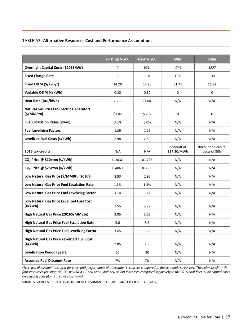
The cost and performance assumptions for the alternative technologies are listed in Table A3. For comparison to existing NGCC

units, capital costs were not included as these costs would typically not be included in a decision to operate or idle an existing power

generating unit. Doing this allows us to better understand the market dynamics of existing resources. However, when comparing

coal units to a new NGCC, wind, or solar unit, we included capital and financing costs for these alternative resources.

To calculate natural gas fuel costs at both existing and new NGCC units, we included assumptions for fuel escalation rates and

levelizing factors to arrive at a levelized fuel cost. The use of fuel escalation rates and levelizing factors also allowed us to evaluate

more accurately high and low natural gas price sensitivities to reflect the impact of a change in natural gas price trajectory on

current market dynamics.

Assumptions were largely taken from the National Renewable Energy Laboratory’s (NREL) 2016 Annual Technology Baseline

(Hand et al. 2016) except for fuel prices, escalation rates, and levelizing factors, which were drawn from the Energy Information

Administration’s (EIA) Annual Energy Outlook for 2017 (EIA 2017a). For wind and solar resource cost assumptions, we assume

the federal production tax credit (PTC) applies to wind and the investment tax credit (ITC) applies to solar resources. Solar costs are

expressed in Alternating Current and are for a fixed axis system.

To account for regional variations in cost and performance, regional multipliers were developed based on data extracted from

NREL’s Regional Energy Deployment System (ReEDS) model as detailed in the 2016 ReEDS model documentation (Eurek et al.

2016) and based on UCS’s reference case modeling runs completed in 2017. Finally, assumed regional capacity factors for wind

and solar resources are also based on data extracted from the ReEDS model inputs and outputs from UCS’s reference case modeling

runs completed in 2017.

To derive an assumed capacity factor for potential replacement wind and solar resources located in geographic proximity to the

coal unit in question, we averaged capacity factors for new-build wind and solar resources in our ReEDS reference case in the same

ReEDS region (or surrounding regions) in which the coal unit is located. By taking this approach, we could align the assumed

potential for wind and solar resources with the geographic location of the coal unit in question.

ASSUMPTIONS REGARDING OUR SENSITIVITIES

We also analyzed the economic competitiveness of coal units under a variety of sensitivities, including high and low natural gas

prices and a $10/ and $25/ton price on CO2 emissions. High and low natural gas prices are drawn from EIA’s Annual Energy


Outlook 2017 using the High and Low Oil and Gas Resources cases respectively. The $10 and $25/ton CO2 prices represent a

conservative range of prices reflected in utility resource planning as reported in Joseph Kruger’s 2017 review of utility integrated

resource planning efforts (Kruger 2017). Under the carbon price scenario, the price on carbon was applied to both NGCC and coal

units. Our methodology and assumptions other than natural gas prices and assumed carbon prices remain constant for our alternative

scenarios to allow for appropriate comparison.

ASSESSING CURRENTLY INSTALLED POLLUTION CONTROLS FOR THE 2016 OPERATING COAL FLEET

To better understand today’s coal fleet and the change it has undergone since 2008, we also looked at pollution controls installed on

each coal unit that we evaluated with the economic stress test. This allows us to better understand how the coal fleet is changing

over time with regard to pollution controls and to understand differences in the characteristics of each category of units

(Announced, Uneconomic, and Remaining). Information on installed pollution controls was drawn from Synapse’s Coal Asset

Valuation Tool (CAVT) (Synapse Energy Economics 2015). If a unit was absent from this dataset, our secondary source for

currently installed pollution controls was the EPA’s National Electric Energy Data System (NEEDS) version 5.15 (EPA 2016a).4

Units were referenced individually to collect information on pollution controls for nitrogen oxides (NOx), sulfur dioxide (SO2),

particulate matter, and mercury.

LIMITATIONS AND UNCERTAINTIES

The US electric power system is dynamic and complex. Any macrolevel economic analysis of the possible fate of individual power

providers is inherently uncertain. Our analysis is not a prediction of what will happen to the US coal power fleet, but rather an effort

to identify those coal generators that are most vulnerable to the current and near-term economic conditions in their respective power

markets. We do not attempt to analyze the dynamic power market conditions of each coal unit that will ultimately influence the

decisionmaking of unit owners or operators. Factors such as the availability of alternative resources; whether the coal unit is owned

by a regulated utility that can recover above-market prices from ratepayers or a merchant regulator subject to wholesale market

price fluctuations; a coal unit’s location on the power grid and its contribution to meeting peak demand or reliability requirements;

how investors are accounting for future costs; and local and regional policy priorities can each weigh heavily on a unit owner’s

decision to retire or continue operating any particular coal unit.

Our analysis also represents a relatively narrow slice of time, attempting to look at the current market forces and economic

competitiveness of coal units today rather than a more holistic, forward-looking, and longer-term assessment of each unit’s

economic viability compared to alternative resources. As fuel prices, capital costs, and other key factors shift, so too will the

economic competitiveness of individual coal units. Further, retiring uneconomic units and replacing them with cleaner alternatives

will happen over a period of several years, making this analysis informative rather than determinative.

Proximity Analysis

The proximity analysis component was intended to provide a high-level screen of the communities living near coal plants. Given the

magnitude of the transition underway—including that which has already occurred, as well as that which is still to come—this

analysis aimed to illuminate the ways in which the coal fleet transition is progressing through communities across the country. The

assessment was composed of a summary of the total population living within a three-mile radius of a coal unit, as well as the

minority (all other than non-Hispanic, white-alone individuals, as defined by the US Census) and low-income (at or below double

the federal poverty level) shares of that population. As a result, the proximity analysis provided only an initial high-level screen for

characterizing possible large-scale trends; though it pulled from the EPA’s EJSCREEN Tool (EPA 2016b), it was not itself an

environmental justice analysis.

This section of the technical document contains a detailed explanation of the methods used to conduct the proximity

analysis, a listing and explanation of the data sources used, and a consideration of the method’s assumptions and limitations.

4 We were not able to determine the presence of pollution controls on seven units that did not appear in either database.


APPROACH

This work followed the proximity analysis methodology

established for the EPA’s EJSCREEN Tool and applied in the

agency’s 2015 EJ Screening Report for the Clean Power Plan

(EPA 2015). The methodology is detailed in the agency’s most

recent technical report, EJSCREEN Environmental Justice

Mapping and Screening Tool: EJSCREEN Technical

Documentation—Draft (EPA 2016c), and summarized here.

At a high level, this analysis was designed to determine

the total population, minority population, and low-income

population living within three miles of each coal unit of focus.

Because these demographics are reported at a geographic

resolution different from that of a three-mile buffer (see, e.g.,

Figure A1), however, the analysis required calculating a

population-weighted average to approximate the population

findings.

Specifically, this proximity analysis drew upon

demographic data available at the census block group level,

which can range widely in area and shape. A three-mile buffer

could capture many block groups in a densely populated area

or just one to a few block groups in a rural area. This proximity analysis combined the demographics data for multiple block groups

by calculating a population-weighted average.

When block groups are completely contained within a buffer, the data can be aggregated as is. However, when a buffer

bisects a block group, the implicated population must be apportioned between that which falls inside the buffer and that which falls

outside. This analysis apportioned intersected block groups by weighting the block groups according to the census blocks—one

level of resolution finer than census block groups—that had centroids falling within the buffered portion of the block group

(Chakraborty, Maantay, and Brender 2011). Such an apportionment approach allows for recognition of variations in population

density across a census block group; however, it cannot identify whether pockets of specific demographics exist in one part of a

block group as opposed to another. These and additional limitations are considered further below.

A final complication is that the date of collection differs for the various levels of resolution. This analysis, by way of the

EJSCREEN v3 geodatabase (EPA 2016b), relied on the American Community Survey (ACS) 2010–2014 dataset for minority and

income information. However, this information is reported out only at the census block group level. Census block data, on the other

hand, are collected only decennially; therefore, the population-weighted average included a scaling adjustment to recognize the

change in population from the 2010 Census to ACS 2010–2014. There are also additional uncertainties introduced by the ACS data,

as the census provides a complete count at one point in time while the ACS collects a stratified random sample of more than

200,000 households each month, here aggregated in the five-year summary form.

The final proximity analysis calculation can be summarized for the population of a given demographic value within a

study area A as follows (EPA 2016c; Krieger et al. 2016):

𝑉𝑎𝑙𝑢𝑒(𝐴) = ∑

𝐵𝑙𝑜𝑐𝑘𝑃𝑜𝑝10𝐵𝐺𝑃𝑜𝑝10

∗ 𝐵𝐺𝐴𝐶𝑆𝑃𝑜𝑝 ∗ 𝐵𝐺_𝑅𝑎𝑤𝑉𝑎𝑙𝑢𝑒

∑𝐵𝑙𝑜𝑐𝑘𝑃𝑜𝑝10

𝐵𝐺𝑃𝑜𝑝10∀𝐵𝑙𝑘,𝐵𝑙𝑘∩𝐴 ∗ 𝐵𝐺𝐴𝐶𝑆𝑃𝑜𝑝

∀𝐵𝑙𝑘,𝐵𝑙𝑘∩𝐴

Here, BlockPop10 refers to the 2010 Census block-level population, BGPop10 refers to the 2010 Census block group-level

population, BGACSPop refers to the ACS 2010–2014 block group–level population estimate, and BG_RawValue refers to the ACS

2010–2014 block group–level raw demographic indicator value.

The resulting output generates, per coal unit point location, the total estimated population within a three-mile radius as

well as the percentage share of the low-income and minority populations. The EJSCREEN tool also generates the associated

FIGURE A1. Illustrative Census Block Groups within a Radius Around a Point

Figure from EPA (2015) shows how census block groups may be

included or excluded from a defined radius around a given point

(see text).

SOURCE: EPA (2015)


percentile for each raw value at the state, regional, and national levels. These percentiles generally convey the percentage of the

national (or state, or regional) population living in a block group with a lower value (EPA 2016c).

This analysis relied on the EPA’s EJSCREEN batch tool script (EPA 2016d), as provided by the agency in May 2017, for

the final unit-level and power plant–level output values. For total population numbers, however, this analysis relied on a separately

generated, though similarly calculated, process. This was conducted via ArcGIS and performed to capture the adjusted census

blocks a single time nationwide in order to avoid double counting between colocated units and colocated or adjacent (i.e., with

overlapping buffers) power plants.

CHARACTERIZATION OF PROXIMITY ANALYSIS FINDINGS

After gathering data on two demographic variables (low-income and minority population living within three miles of a coal

generating unit), we built a national picture of the demographics of communities with coal-fired power plants aggregated by current

and future operational status of those coal units. Specifically, the EJSCREEN batch tool script provides the raw values5 for each

demographic variable—that is, the percentage of the total population living within three miles of the specified unit location that is

identified as minority (that is, all other than non-Hispanic, white-only individuals) and also the percent low income (defined

as twice the federal poverty level). Importantly, EJSCREEN also puts these raw values in the context of the state, region, and nation

by providing the percentile value for each study area in each of these three geographic breakdowns. This makes it simpler to

compare how a given community ranks compared to the full population of the state or EPA region where it is located or to the

national population. Thus, a coal plant community ranking in the 20th percentile for its state implies that 20 percent of the census

blocks in the state would rank lower in terms of minority population.

These percentile rankings can vary significantly when considered relative to the state or national values. This analysis

focuses on the state percentiles for each coal plant community because comparing to the national averages or medians might mask

demographic differences among states. For example, consider a state with a lower average minority population compared to the

national average; a given coal plant community in that state might have a higher proportion of minority residents by state standards,

but that information might be missed by comparing to the national average. Figure A2 illustrates the differences between the state

and national demographics for the communities surrounding the entire US coal fleet in 2008 and 2016.

To provide context for the demographic and income data we gathered, we present the information in terms of how it

compares to the rest of the population in the state. Specifically, we note whether a value falls above or below the state’s median,

which is calculated here as half the population in the state living in a community6 with a lower data point. In other words, for the

aggregation of coal units by current and future operating status, we tabulate whether the surrounding community has a state

percentile for each demographic variable that is above the 50th percentile. This effectively compares the coal unit community's

ranking in each demographic indicator separately to the state median for each indicator.

DATA SOURCES

The proximity analysis relied on a range of data sources, as recorded here.

The analysis itself was conducted for each coal unit identified according to the “Characterizing the 2008 Coal Fleet” and

“Characterizing the 2016 Coal Fleet” sections above. Latitude and longitude information for each unit was determined via S&P

Global (2017) and cross-checked with EIA’s generator inventory based on Form EIA-860 (EIA 2016).

Total population and block group values were taken from ACS 2010–2014, via EJSCREEN v3 (EPA 2016b). Census

blocks were available from the 2010 Census, as population at that geographic resolution are collected and distributed only

decennially.

Unit-level analyses were conducted using the EJ Screen batch tool (EPA 2016d), run using ArcGIS. National population

figures were calculated directly through ArcGIS applying the same population-weighted average approach, but excluding overlaps

in buffers to avoid double counting.

5 EJSCREEN provides a number of other demographic variables that were not considered in this analysis. 6 Here, community refers to census block groups, which are Census-designated areas typically containing between 600 and 3,000 people.


ASSUMPTIONS AND LIMITATIONS

The proximity analysis was intended to assist in characterizing, at a national level, the communities living near coal units and to

shed light on how the transition of the coal fleet more broadly has been playing out for these communities across the country.

Critically, the proximity analysis is not intended to be an environmental justice analysis (e.g., Declet-Barreto et al. 2017; Wilson et

al. 2012). Still, this effort has played a beneficial role in informing what a just transition must consider as policies are designed to

cut pollution and support and strengthen these communities over time. It brings people into the equation.

It is critical to acknowledge the limitations of this specific approach, as well as the risks of insufficiently grounding the

limitations of the resultant findings. In particular, a national-level screen cannot address the fact that every single community, and

adjacent coal plant, is different. Between differences in plant sizes, operation styles (e.g., peaking vs. steady operations), specific

fuel types, and pollution controls, to community settlement patterns, presence (or absence) of additional pollution sources, economic

diversity and access, and more, it is critical to recognize that what applies in one location may not apply in another. Therefore, this

analysis is intended to inform at a high level, not at a community-specific level. Recognizing that limitation, we highlighted

different qualitative aspects of the transition through four community snapshots, described in the accompanying fact sheet and

available in an interactive web feature at www.ucsusa.org/communitysnapshots.

FIGURE A2. Share of Minority Population Located Near Coal Units Compared to the State and National Median

This chart shows the share of coal unit communities—defined as the population living within three miles of a coal generator—with a minority

population above the median. It also illustrates the difference in this share, depending on whether a comparison is made to the state median

value or the national median value. The dark red bars show the fraction of coal unit communities (in 2008 and 2016) that are above the state

median minority population; the light red bars show the fraction that are above the national median. In other words, in 2016, 38.1 percent of

coal units were in communities that were above their respective state medians in terms of the fraction minority population, whereas 23.4

percent topped the national median.

http://sharepoint.ucsusa.org/programs/ce/ProjectsandCampaigns/Power%20Ahead/Analytics/Clean%20Energy%20Transition%20Analysis%20FY17/Release%20Materials/www.ucsusa.org/communitysnapshots


Additionally, the characterization of those living within three miles of a coal unit captures only one segment of the

population affected by coal plant operations. The negative effects of coal operations are far reaching, from power plant pollutants

that travel to communities located hundreds of miles away, to negative effects arising from associated coal-fired generation

activities, such as dust generated by coal transport from mine to plant, the disposal of coal ash waste, or upstream health and

environmental impacts on coal mining communities. This proximity analysis was not intended to be a public health study or even an

approximation of health impacts. Instead, it is a screen of communities living within close proximity of a coal plant, intended to

inform about that which has already occurred, as well as to help guide policymaking in anticipation of what might happen in the

future. Importantly, a proximity analysis cannot address questions about why there may be disparities in plant location in the first

place, e.g., whether a coal plant was located in a low-income community originally or whether only low-income communities

developed after construction.

The proximity analysis followed previous methodological approaches (Krieger et al. 2016; EPA 2015). Still, the design of

the proximity analysis itself does have limitations. First, by applying a buffer approach, the analysis had to include a population-

weighted average to capture partially contained areas (see methodology detailed above). This allowed for a potentially fuller

analysis than simply characterizing the census block group within which a coal unit fell; however, it also introduced a range of

uncertainties. Most important among these is that while the use of block-level centroids allowed for a strong estimate of population

density within captured and excluded areas, it could not inform whether specific demographic pockets existed within a census block

group, as the block-level information captured only population, not additional demographics. However, it was ultimately deemed

preferable to either a real apportionment or simple block group–level association.

Two additional caveats are directly related to the data. First, though the coal fleet is tracked over time, the proximity

analysis was conducted for a single snapshot, namely, using ACS 2010–2014 (and 2010 Census data for apportionment). This was

an intentional decision to standardize findings; however, it would fail to capture any significant demographic changes that could

have occurred in a community immediately after a coal plant closure, should that closure have occurred in the early years of this

analysis. Second, for income characterization, the ACS reports findings only as a share of those for whom income status was

determined. This frequently means that some small subset of the population is omitted.

Finally, this proximity analysis is organized around coal units. That means that a community could be characterized

multiple times if more than one unit is located at a single site. When characterizing the communities in which coal units are located,

such an approach makes sense. However, the analysis also aggregated findings to the plant level—and the national, no-overlapping-

buffers level—for specific conclusions and characterizations. Additionally, the analysis did not track the communities in which a

new power plant was built after a plant in a different community was closed. This is a significant and important outcome arising

from the energy system transition more broadly; however, this analysis focused solely on the transition of the coal fleet itself.


Detailed Results and Findings


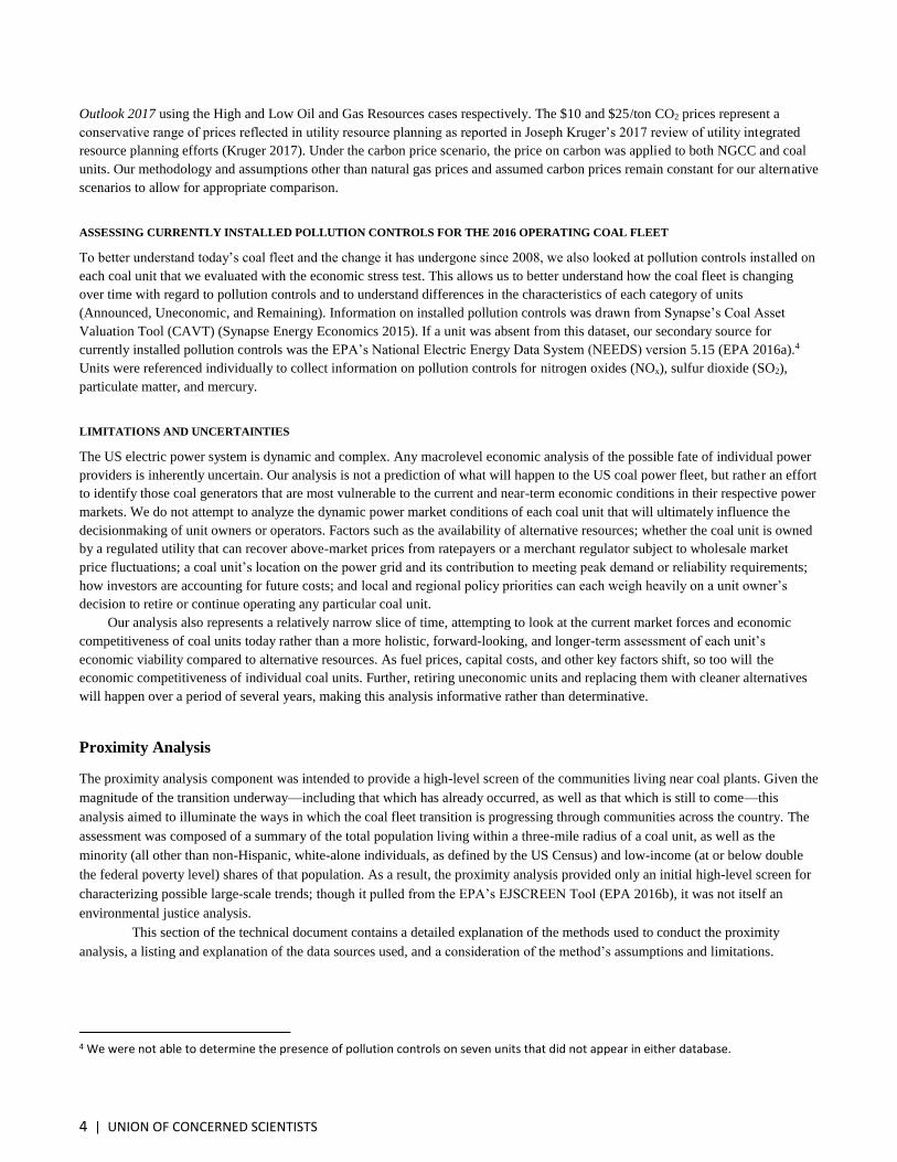
Figure A3 shows the results of our economic stress test under the various scenarios. When comparing each coal unit’s current cost

of generating electricity to the cost of generating electricity from an existing NGCC unit, 20 percent of the 2016 coal fleet—122

units representing 57 GW of capacity—is uneconomic, meaning its costs are higher than that of an existing NGCC unit. When

combined with 163 coal units representing 51 GW of capacity that have already announced plans for retirement or conversion to a

different fuel source, 38 percent of today’s coal fleet faces an uncertain near-term future. Under current operating costs, 36 coal

units totaling 9.3 GW are also uneconomic compared to regional onshore wind resources and 17 units totaling 2.2 GW are

uneconomic compared with regional utility-scale solar PV. Coal units face the least pressure from new-build NGCC units. Only 6

units totaling 2.2 GW of capacity are uneconomic compared to new NGCC.

The economic competitiveness of the nation’s coal fleet changes significantly with only modest changes in cost assumptions.

Under our low natural gas price scenario, the number of units that are uneconomic compared to existing NGCC grows to 169,

representing 75 GW of capacity, or 26 percent of the 2016 fleet. Further, when we assume a $10/ton price on CO2 emissions as a

proxy for potential carbon regulation or a host of other potential cost increases that might impact fossil fuel power generation in the

FIGURE A3. Sensitivity of Uneconomic Coal Capacity Compared to Different Alternative Resources

Each bar shows the amount of uneconomic coal capacity in GW compared to alternative resources, including existing NGCC, new NGCC,

wind with the production tax credit (PTC), and solar with the investment tax credit (ITC). Reference case cost assumptions are shown in red,

and each additional color shows how much more coal is uneconomic under different cost assumptions.


near term,7 the number of coal units (and the capacity they represent) that are uneconomic compared to wind and solar resources

grows substantially. Under an assumed $10/ton price on CO2, 99 units representing 40 GW of capacity are uneconomic compared to

regional wind resources. Similarly, 21 units representing 2.8 GW of capacity are uneconomic compared with regional solar

resources under this scenario. When the price on CO2 is increased to $25/metric ton, 62 percent of the 2016 coal fleet—371 units

totaling 175 GW of capacity—are uneconomic compared to regional wind resources. A summary of results of our economic stress

test scenarios can be found in Figure A3 and Table A4.

The ongoing transition away from coal most heavily affects smaller and less-frequently run coal units. A look at the size and

capacity factors of the 2016 coal fleet shows that those units likely to remain economically competitive into the near future are

larger units, with an average size of 510 MW compared to 469 MW for those that were uneconomic and 317 MW for announced

retirements and conversions (see Table A5). Uneconomic units also ran less often: operating at a 2016 capacity factor of 41 percent

compared to 58 percent for those units that passed our economic stress test. Those units already announced for retirement were the

smaller, older units of the 2016 fleet that ran the least often, with an average capacity factor of 35 percent and an average age of 49

years.

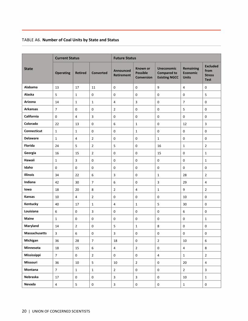
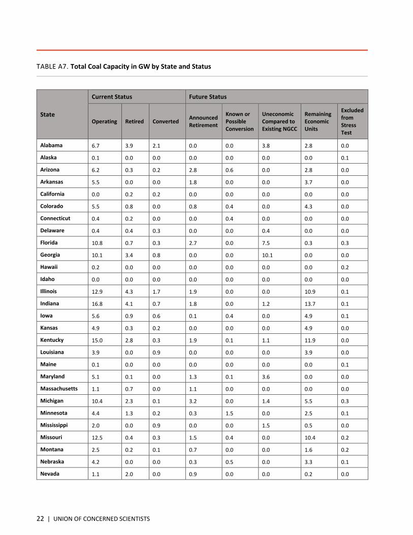
Tables A6, A7, and A8 show the characteristics of the 2008 and 2016 coal fleets by state in terms of number of units, capacity,

and generation, respectively.

Estimate of Monetized Value of Emissions Reductions

We calculated a rough estimate of the change in emissions at the national level based on the coal fleet characterized above. By

aggregating emissions data (S&P Global 2017) for SO2, NOx, and CO2 for all the coal units in the 2008 fleet, we estimate the

emissions reductions from these 1,256 units between 2008 and 2016 as a result of the combination of coal retirements, conversion to

other fuels, change in usage, and pollution control equipment installed in response to environmental standards; we found an 80

percent reduction in SO2, a 64 percent reduction in NOx, and a 34 percent reduction in CO2. Since this estimate focused only on the

coal fleet, it does not capture any increase in emissions from new natural gas power plants.

To estimate the monetized value of these aggregated emissions reductions, we calculate the amount of each pollutant reduced

between 2008 and 2016 from the 1,256 units we identified and then multiply by the value of emissions reductions for each

pollutant. To estimate the costs of SO2 and NOx, we used the per-ton estimates calculated by the EPA (2013). For the benefits of

CO2 reductions, we use the social cost of carbon updated in 2016 (Interagency Working Group 2016). Assumptions are summarized

in Table A9. Based on the change in emissions from 2008 to 2016 from these 1,256 coal units, we estimate public health benefits of

$211 billion from SO2 reductions, $9.4 billion from NOx reductions, and $30 billion from CO2 reductions, for a total of $250 billion.

Pollution Controls on the 2016 Coal Fleet

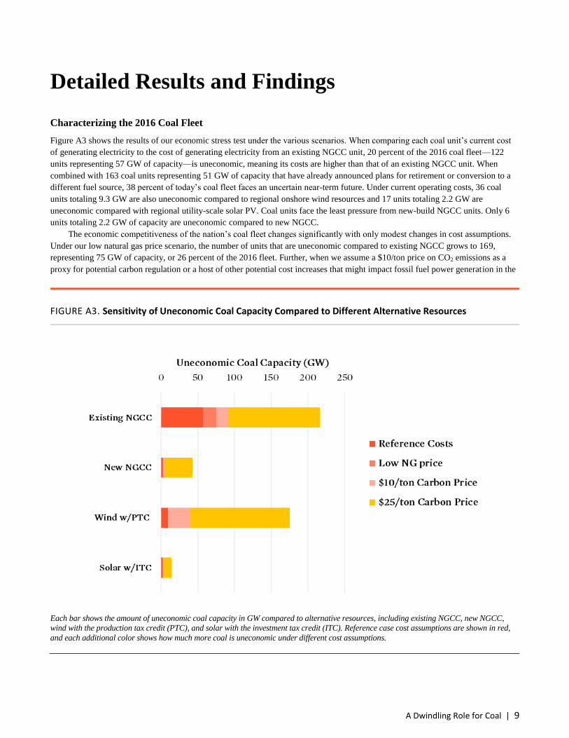
We also looked at missing pollution controls on each unit in the 2016 coal fleet. Figure A4 shows the percentage of units in each

category (Announced, Uneconomic, and Remaining) that are missing pollution controls for each of four criteria pollutants: NOx,

SO2, particulate matter, and mercury (Hg).8 Multiple controls are available for each of these pollutants, some performing better than

others at reducing emissions. However, for purposes of this snapshot, we simply looked at whether any one of the available control

technologies for each pollutant has been installed at a particular coal unit. The most common controls are wet flu gas desulfurization

for SO2, selective catalytic reduction for NOx, baghouses for particulate matter, and activated carbon injection for mercury.

In all categories of pollutants other than particulate matter, a higher percentage of units already announced for retirement did

not have controls installed, and nearly 20 percent of announced units had no controls installed for any of the pollutants, compared

with 3 percent and 6 percent for uneconomic and remaining units respectively. However, comparison of uneconomic versus

7 For example, increase in delivered cost of fuel, the imposition of increasingly stringent environmental standards, or increased O&M costs as the coal fleet ages. 8 There are a variety of pollution controls that can be installed to reduce emissions of these pollutants. For our evaluation, we report whether a unit has any one of the various technologies that can be installed to reduce emissions of a pollutant. It should also be noted that some controls can be used individually or in combination to reduce emissions of multiple pollutants, thereby potentially eliminating the need for other control technologies to comply with current regulations.


remaining units varied depending on the pollution control: a higher percentage of uneconomic units lacked controls for particulate

matter and mercury, while a higher percentage of remaining units lacked controls for SO2 and NOx.

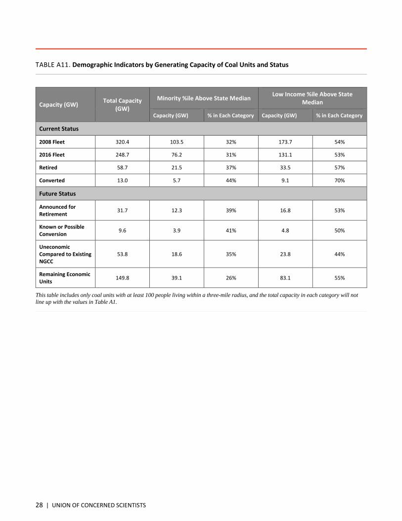
Findings from Proximity Analysis

As described earlier, the units were aggregated according to current and future status and according to whether the surrounding

community had a minority percentile or low-income percentile above the state's median value. These results are tabulated in Table

A10 for the number of coal units, Table A11 for the total capacity in GW, and Table A12 for the total generation in gigawatt-hours

(GWh). Following the methodology set out by the EPA in its Clean Power Plan EJSCREEN analysis (EPA 2015), units that are

surrounded by fewer than 100 people living within a three-mile radius are ignored. This is why the totals in these tables will not

match those shown in Table A1; for example, only 1,178 of the 1,256 coal units identified as operating in 2008 have at least 100

people living within three miles.

The percentages shown in Tables A10 through A12 are relative to the totals for each status category. Thus, for example, in

Table A10, the 2016 operating coal fleet represented 248.7 GW of capacity, of which 31 percent (76.2 GW) were located in

communities with a higher percentage of minority residents than the state median and 53 percent (131.1 GW) were located in

FIGURE A4. Fraction of Units Missing Pollution Controls

Units already announced for retirement typically have a higher chance of lacking pollution controls installed for SO2, NOX, or mercury.

However, as we look ahead, we find a higher percentage of units considered uneconomic compared to existing NGCC units lack pollution

controls for particulate matter and mercury compared with our remaining units. Conversely, a higher percentage of remaining units lack

controls for SO2 and NOx compared with uneconomic units.

SOURCES: SYNAPSE ENERGY ECONOMICS (2015); EPA (2015A).


communities with a higher percentage of low-income residents than the state median. Note that these two groupings are not

mutually exclusive; some coal plant communities fall above the state median in both categories, and some meet neither threshold.

We sought to test whether the disparities in the location of coal units in minority and low-income communities has been

alleviated in the transition away from coal from 2008 to 2016 and whether there was any hint that it might change in the future as

more coal units face early retirement. For this calculation, we followed the methodology developed by the EPA in its EJ Screening

Report for the Clean Power Plan (EPA 2015). The statistical question was: How often do study area demographics exceed state

median demographics? We evaluated this question using a two-sample t-test assuming unequal variances and compared the state

percentile for each demographic from the 2008 coal unit fleet to those of the 2016 fleet. We detect no statistically significant change

in the average percentile of the fraction of minority residents living within three miles of an operating coal unit from 2008 to 2016.

We observe a barely statistically significant decrease in the average percentile of low-income residents during that time, but that

apparent gain is erased when including the units that converted to another fuel over that time.

We conducted a similar test looking at the potential future based on units that face early retirement. For this test, we

compared the state percentile for each demographic from the 2016 coal unit fleet to those of a potential future coal fleet: coal units

that would be left after both announced retirements and conversions and after units uneconomic compared to existing NGCC go

offline. For this potential future fleet of coal units, we include the units that were excluded from the economic stress test, making a

conservative assumption that these units would remain online and continue to affect the communities where they are located. We

find no statistically significant difference between the 2016 fleet and this potential future fleet in terms of either demographic

variable.

Our results show that the fraction of coal units in low-income and minority areas has not changed significantly from 2008

to 2016 and is not anticipated to change significantly in the future based on our economic stress test calculation of which units face

early retirement.

As described above, there are multiple ways to evaluate our results—in terms of number of units, total capacity, or total

generation and in terms of how much of each are found in coal plant communities where one of the two demographics is above the

state median. The analysis also looked at state-level breakdowns of these metrics. These comparisons are more challenging, mostly

because some states have only a few coal generators, so the percentage of those units (or capacity or generation) located in low-

income or minority communities is less statistically meaningful.

Table A13 shows one way of disaggregating the proximity analysis by state. The table shows the 2016 generation from

coal units identified as operating at the end of 2016. It also shows explicitly how much of that generation is in areas with at least

100 residents living within three miles (the amount of coal generation "evaluated" using the proximity analysis), as well as the

amount of coal generation that is uneconomic relative to existing NGCC and also in areas with at least 100 residents. The

percentages in the rightmost four columns indicate the generation in communities with a percentage of minority and low-income

residents, respectively, above the state median, relative to the coal generation that was evaluated with the proximity analysis. For

states that have coal units located in less rural areas, the table indicates how much of the currently operating coal fleet is in minority

and low-income communities and similarly how much of the generation found to be uneconomic compared to existing NGCC is in

these communities.

Replacement Generation Potential

With such a large amount of coal generation potentially facing retirement, we sought to understand what resources could be

expected to come online through 2025 to make up for any shortfall in meeting demand. Here we provide a cursory review of the

generation resources that can reasonably be expected to come online in the near future. It is important to note that this is not a

reliability analysis, nor does it take into account potential transmission or natural gas distribution constraints.

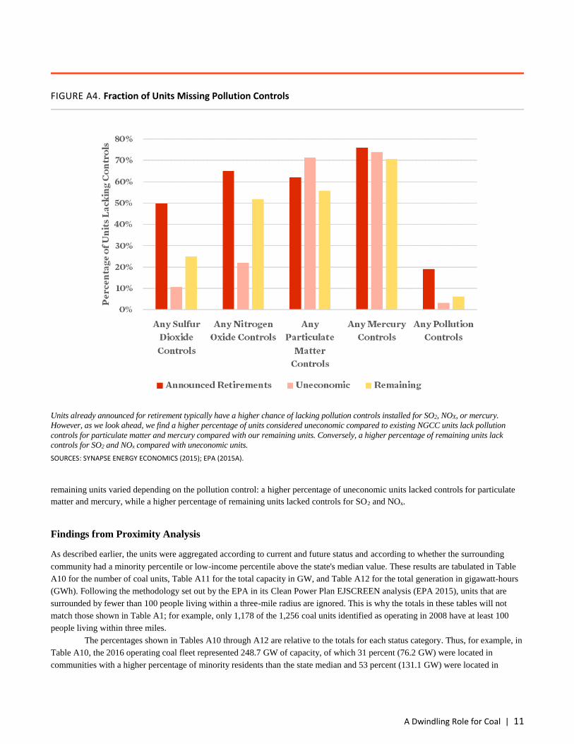
First, the potential lost coal generation is tabulated by NERC region; we sum 2016 generation from those generators that

have announced they will retire through 2025 (but excluding those that plan to convert to natural gas or be replaced with new

natural gas) combined with the generators identified as uneconomic compared to existing NGCC. See Tables A14 and A15 for a

tabulation by region of 2016 coal unit capacity and generation, respectively. This potential lost generation is shown by the gray bars

in Figure A5. The Southeast (SERC) as well as the Mid-Atlantic and Great Lakes (RFC) regions stand out as having the most coal

generation potentially going offline. To estimate the potential for replacement generation, we considered four additional sources of

new generation expected to come online: state-mandated Renewable Electricity Standards (RESs), state-mandated Energy


Efficiency Resource Standards (EERSs), under-construction nuclear power plants, and new NGCC builds. RES data comes from the

Lawrence Berkeley National Laboratory's estimate of cumulative expected RES demand in 2025 (LBNL 2017). One limitation of

this calculation is an imperfect match between states and NERC regions; a rough estimate was made to assign RES demand to

NERC region. Avoided generation from state EERSs is based on UCS calculations of the additional avoided generation beyond

what is captured in the EIA Annual Energy Outlook (EIA 2017a); these requirements are derived from the EPA's now archived

database on state programs (EPA 2014). Nuclear generation is estimated for under-construction nuclear plants in Georgia and

Tennessee; the potential contribution from the V.C. Summer plant in South Carolina is excluded following the August 2017

announcement that the project has been abandoned. New NGCC builds labeled as under construction or in advanced development

(S&P Global 2017) are also included, and generation is estimated using the 2016 capacity factor for existing NGCC plants of 56

percent (EIA 2017b).

We found that in most regions of the country these sources of anticipated generation alone are sufficient to make up lost

coal generation. It is also likely that this calculation underestimates the contribution from new renewable resources, in that it

considers only state-mandated renewables and energy efficiency and not new investments that may be developed strictly on

economic grounds. For example, Texas has installed significant and economically competitive wind resources far in excess of its

FIGURE A5. Potential Loss in Coal Generation Compared to Anticipated Additional Generation

The potential loss in 2016 coal generation due to announced retirements (in black) and uneconomic units compared to existing NGCC (in

gray) compared with an estimate of anticipated new generation by 2025 from RES (dark green), EERS (light green), nuclear (yellow), and new

NGCC (dark blue). Also shown is additional existing NGCC generation (light blue) that could be tapped to meet shortfalls in SERC and FRCC

(see text). Key to NERC regions: ReliabilityFirst Corporation (RFC); Southeast Reliability Corporation (SERC); Texas Reliability Entity

(TRE); Western Electricity Coordinating Council (WECC); Southwest Power Pool (SPP); Midwest Reliability Organization (MRO); Florida

Reliability Coordinating Council (FRCC); and Northeast Power Coordinating Council (NPCC).


RES. The SERC and Florida (FRCC) regions show large shortfalls, which is not an unexpected result given that nearly all coal units

in the region did not meet the economic stress test (see Figure 3 in the accompanying fact sheet) and the region as a whole generally

has weak or nonexistent policies to drive new investments in renewables and efficiency. However, as Figure A5 shows, both regions

have sufficient excess existing natural gas generation to make up for the potential shortfalls (light blue portions of bars). FRCC

would require a slight increase in the capacity factor of existing NGCC units (from 58 percent to 59 percent), while SERC’s

shortfall would imply a 17 percent increase (to 72 percent), implying that the region is at risk for an over-reliance on natural gas

(Deyette 2015).

NERC’s most recent Long-Term Reliability Assessment confirms that coal and other planned power plant retirements do

not pose a threat to reliability9 (NERC 2016). NERC projects that all regions of the country will have more than enough power plant

capacity to greatly exceed their targeted reserve margins through at least 2021 (see Figure A6). In particular, NERC shows

significant excess capacity in SERC, FRCC, and RFC (shown as PJM for PJM Interconnection)—the regions where our analysis

finds the vast majority of uneconomic coal units compared to existing natural gas. NERC also estimates significant excess capacity

in these regions and most other regions through 2026.

9 NERC’s estimate of anticipated resources includes new capacity additions that have completed or are under construction, have a power purchase agreement or contract, are included in utility integrated resource plans, or are under a regulatory environment that have resource adequacy requirements. NERC’s estimate of prospective resources includes capacity that has been requested but that has not received approval for planning requirements.

FIGURE A6. NERC Reliability Assessment

This chart shows anticipated reserve margin (dark blue), which is NERC’s primary metric used to evaluate projected resource adequacy to

meet expected electricity load. The horizontal black lines indicate the reference margin level for each region; if anticipated resources fall

below this line, it could indicate a risk to reliability. This is NERC’s assessment for 2021, reflecting NERC’s five-year assessment of available

capacity margins.

This information from the North American Electric Reliability Corporation’s website is the property of the North American Electric Reliability Corporation and is available at http://www.nerc.com/pa/RAPA/ra/Reliability%20Assessments%20DL/2016%20Long-Term%20Reliability%20Assessment.pdf.

This content may not be reproduced in whole or any part without the prior express written permission of the North American Electric Reliability Corporation.

SOURCE: FIGURE 1.2 FROM NERC (2016).


Data Tables

TABLE A1. Summary of Current and Future Status of 2008 and 2016 Coal Fleets

Coal Unit Category Number of Units Capacity (GW) Generation (GWh)1

Number % of Total Capacity % of Total Generation % of Total

Current Status (in 2016) of 2008 Coal Units

Operating 706 56% 284.1 80% 1,646,917 83%

Retired 452 36% 59.3 17% 274,891 14%

Converted 98 8% 13.4 4% 68,126 3%

TOTAL 1256 356.7 1,989,935

Future Status of 2016 Operating Coal Units

Announced for Retirement 128 18% 38.1 13% 118,244 10%

Known or Possible Conversions 35 5% 12.8 5% 44,113 4%

Uneconomic Compared to Existing NGCC 122 17% 57.2 20% 225,768 19%

Remaining Economic Units 337 48% 171.8 60% 823,111 68%

Excluded from Economic Stress Test 84 12% 4.2 1% 5,029 0.4%

TOTAL 706 284.1 1,216,265

Each unit in the 2008 coal fleet is assigned a current status (as of the end of 2016) of Operating, Retired, or Converted. For the 2016

Operating coal fleet, we assign a potential future status as Announced for Retirement, Known or Possible Conversions, Uneconomic compared

to existing natural gas units (i.e., Ripe for Retirement), Remaining Economic Units (i.e., those that pass the economic stress test), or Excluded

from the Economic Stress Test (i.e., insufficient data to compare costs).

1 This table provides 2008 generation values for the upper section on the Current Status of the 2008 fleet, and 2016 generation values for the lower section on the Future Status of the current fleet. Totals may not add due to rounding.

SOURCE: BASED ON DATA FROM S&P GLOBAL (2017).


TABLE A2. Coal Unit Operations and Maintenance (O&M) Cost Assumptions

Unit Capacity (MW)

<100 100–300 >300

Fixed O&M (2016$/kW-yr) 33.05 23.14 19.83

Variable O&M (2016$/MWh) 5.51 4.41 4.13

SOURCES: FISHER & BIEWALD (2011); NERC (2010).


TABLE A3. Alternative Resources Cost and Performance Assumptions

Existing NGCC New NGCC Wind Solar

Overnight Capital Costs ($2016/kW) 0 1031 1741 1827

Fixed Charge Rate 0 11% 10% 10%

Fixed O&M ($/kw-yr) 14.20 14.20 51.71 15.92

Variable O&M (¢/kWh) 0.30 0.30 0 0

Heat Rate (Btu/kWh) 7655 6660 N/A N/A

Natural Gas Prices to Electric Generators ($/MMBtu) $3.02 $3.02 0 0

Fuel Escalation Rates (20-yr) 3.0% 3.0% N/A N/A

Fuel Levelizing Factors 1.29 1.29 N/A N/A

Levelized Fuel Costs (¢/kWh) 2.98 2.59 N/A N/A

2016 tax credits N/A N/A discount of

$17.80/MWh discount on capital

costs of 30%

CO2 Price @ $10/ton (¢/kWh) 0.2032 0.1768 N/A N/A

CO2 Price @ $25/ton (¢/kWh) 0.4063 0.3535 N/A N/A

Low Natural Gas Price ($/MMBtu; 2016$) 2.93 2.93 N/A N/A

Low Natural Gas Price Fuel Escalation Rate 1.5% 1.5% N/A N/A

Low Natural Gas Price Fuel Levelizing Factor 1.14 1.14 N/A N/A

Low Natural Gas Price Levelized Fuel Cost (¢/kWh) 2.55 2.22 N/A N/A

High Natural Gas Price (2016$/MMBtu) 3.05 3.05 N/A N/A

High Natural Gas Price Fuel Escalation Rate 5.6 5.6 N/A N/A

High Natural Gas Price Fuel Levelizing Factor 1.65 1.65 N/A N/A

High Natural Gas Price Levelized Fuel Cost (¢/kWh) 3.85 3.35 N/A N/A

Levelization Period (years) 20 20 N/A N/A

Assumed Real Discount Rate 7% 7% N/A N/A

Overview of assumptions used for costs and performance of alternative resources compared in the economic stress test. The columns show the

four resources (existing NGCC, new NGCC, new wind, and new solar) that were compared separately to the 2016 coal fleet. Sunk capital costs

on existing coal plants are not considered.

SOURCES: VARIOUS; UPDATED VALUES FROM FLEISHMAN ET AL. (2013) AND CLEETUS ET AL. (2012).


TABLE A4. Summary of Results in Different Scenarios for Economic Stress Test

Scenario Existing NGCC New NGCC Wind Utility Scale Solar PV

Reference Case Costs 57.2 2.2 9.3 2.2

High Natural Gas Price 27.4 0.1 9.3 2.2

Low Natural Gas Price 74.8 2.9 9.3 2.2

$10/Ton CO2 Price 91.7 5.7 40.3 2.8

$25/Ton CO2 Price 216.0 42.6 175.3 13.9

This table shows the amount of existing coal generating capacity in GW compared to each alternative resource (columns) and under each

sensitivity test (rows). For example, in the case in which we assumed a CO2 price of $10/ton, 40.3 GW of coal capacity is uneconomic

compared to wind.

Note: Individual coal units may be uneconomic compared to multiple resources, so numbers shown are not cumulative. In every case, total 2016 coal fleet evaluated by the economic stress test equals 622 units totaling 279.9 GW of capacity. Of that, 163 units totaling 50.9 GW of capacity are already slated for retirement or conversion by 2030. Of the 706 units identified as operating in 2016 in Table A1, 84 units totaling 4.2 GW of capacity were excluded from the economic stress test because of insufficient data.


TABLE A5. Characteristics of 2016 Operating Coal Fleet

Announced

Retirements and Conversions

Uneconomic Compared to Existing NGCC

Remaining Units

Number of Coal Units 163 122 337

Total Capacity (GW) 50.9 57.2 171.8

% of Total US Retail Electricity Sales (2016) 4.4% 6.1% 22.1%

Average Generator Age (Years) 49 41 41

Average Generator Capacity Factor 35% 40% 58%

Average Generator Size (MW) 317 469 510

This table summarizes the characteristics of the units in the 2016 operating fleet that were analyzed using the economic stress test.


TABLE A6. Number of Coal Units by State and Status

State

Current Status Future Status

Operating Retired Converted Announced Retirement

Known or Possible Conversion


Remaining Economic Units

Excluded from Stress Test

Alabama 13 17 11 0 0 9 4 0

Alaska 5 1 0 0 0 0 0 5

Arizona 14 1 1 4 3 0 7 0

Arkansas 7 0 0 2 0 0 5 0

California 0 4 3 0 0 0 0 0

Colorado 22 13 0 6 1 0 12 3

Connecticut 1 1 0 0 1 0 0 0

Delaware 1 4 2 0 0 1 0 0

Florida 24 5 2 5 0 16 1 2

Georgia 16 15 2 0 0 15 0 1

Hawaii 1 3 0 0 0 0 0 1

Idaho 0 0 0 0 0 0 0 0

Illinois 34 22 6 3 0 1 28 2

Indiana 42 30 7 6 0 3 29 4

Iowa 18 20 8 2 4 1 9 2

Kansas 10 4 2 0 0 0 10 0

Kentucky 40 17 1 4 1 5 30 0

Louisiana 6 0 3 0 0 0 6 0

Maine 1 0 0 0 0 0 0 1

Maryland 14 2 0 5 1 8 0 0

Massachusetts 3 6 0 3 0 0 0 0

Michigan 36 28 7 18 0 2 10 6

Minnesota 18 15 6 4 2 0 4 8

Mississippi 7 0 2 0 0 4 1 2

Missouri 36 10 5 10 2 0 20 4

Montana 7 1 1 2 0 0 2 3

Nebraska 17 0 0 3 3 0 10 1

Nevada 4 5 0 3 0 0 1 0


New Hampshire 5 0 0 0 0 4 0 1

New Jersey 6 3 0 4 0 1 1 0

New Mexico 7 4 0 2 0 0 5 0

New York 3 20 4 3 0 0 0 0

North Carolina 27 28 1 9 2 11 0 5

North Dakota 13 0 0 1 0 1 9 2

Ohio 39 50 1 11 5 0 16 7

Oklahoma 10 2 0 1 3 0 6 0

Oregon 1 0 0 0 1 0 0 0

Pennsylvania 29 27 7 0 0 0 16 13

Rhode Island 0 0 0 0 0 0 0 0

South Carolina 12 17 4 0 0 12 0 0

South Dakota 1 1 0 0 0 0 1 0

Tennessee 23 10 0 7 0 2 14 0

Texas 41 2 0 2 0 0 39 0

Utah 9 5 0 0 3 0 5 1

Vermont 0 0 0 0 0 0 0 0

Virginia 18 14 7 2 2 13 0 1

Washington 2 0 0 2 0 0 0 0

West Virginia 19 18 0 0 0 12 6 1

Wisconsin 24 23 5 3 1 0 15 5

Wyoming 20 4 0 1 0 1 15 3

Future status is tabulated only for units that are listed as operating at the end of 2016.

SOURCE: BASED IN PART ON DATA FROM S&P GLOBAL (2017).


TABLE A7. Total Coal Capacity in GW by State and Status

State







Alabama 6.7 3.9 2.1 0.0 0.0 3.8 2.8 0.0

Alaska 0.1 0.0 0.0 0.0 0.0 0.0 0.0 0.1

Arizona 6.2 0.3 0.2 2.8 0.6 0.0 2.8 0.0

Arkansas 5.5 0.0 0.0 1.8 0.0 0.0 3.7 0.0

California 0.0 0.2 0.2 0.0 0.0 0.0 0.0 0.0

Colorado 5.5 0.8 0.0 0.8 0.4 0.0 4.3 0.0

Connecticut 0.4 0.2 0.0 0.0 0.4 0.0 0.0 0.0

Delaware 0.4 0.4 0.3 0.0 0.0 0.4 0.0 0.0

Florida 10.8 0.7 0.3 2.7 0.0 7.5 0.3 0.3

Georgia 10.1 3.4 0.8 0.0 0.0 10.1 0.0 0.0

Hawaii 0.2 0.0 0.0 0.0 0.0 0.0 0.0 0.2

Idaho 0.0 0.0 0.0 0.0 0.0 0.0 0.0 0.0

Illinois 12.9 4.3 1.7 1.9 0.0 0.0 10.9 0.1

Indiana 16.8 4.1 0.7 1.8 0.0 1.2 13.7 0.1

Iowa 5.6 0.9 0.6 0.1 0.4 0.0 4.9 0.1

Kansas 4.9 0.3 0.2 0.0 0.0 0.0 4.9 0.0

Kentucky 15.0 2.8 0.3 1.9 0.1 1.1 11.9 0.0

Louisiana 3.9 0.0 0.9 0.0 0.0 0.0 3.9 0.0

Maine 0.1 0.0 0.0 0.0 0.0 0.0 0.0 0.1

Maryland 5.1 0.1 0.0 1.3 0.1 3.6 0.0 0.0

Massachusetts 1.1 0.7 0.0 1.1 0.0 0.0 0.0 0.0

Michigan 10.4 2.3 0.1 3.2 0.0 1.4 5.5 0.3

Minnesota 4.4 1.3 0.2 0.3 1.5 0.0 2.5 0.1

Mississippi 2.0 0.0 0.9 0.0 0.0 1.5 0.5 0.0

Missouri 12.5 0.4 0.3 1.5 0.4 0.0 10.4 0.2

Montana 2.5 0.2 0.1 0.7 0.0 0.0 1.6 0.2

Nebraska 4.2 0.0 0.0 0.3 0.5 0.0 3.3 0.1

Nevada 1.1 2.0 0.0 0.9 0.0 0.0 0.2 0.0


New Hampshire 0.6 0.0 0.0 0.0 0.0 0.6 0.0 0.1

New Jersey 2.0 0.2 0.0 1.5 0.0 0.3 0.2 0.0

New Mexico 3.7 0.6 0.0 0.9 0.0 0.0 2.8 0.0

New York 1.0 2.4 0.6 1.0 0.0 0.0 0.0 0.0

North Carolina 11.6 3.0 0.0 1.8 1.5 7.9 0.0 0.3

North Dakota 4.3 0.0 0.0 0.2 0.0 0.1 3.9 0.1

Ohio 16.4 7.1 0.1 4.0 2.2 0.0 10.0 0.1

Oklahoma 4.7 1.1 0.0 0.5 1.7 0.0 2.5 0.0

Oregon 0.6 0.0 0.0 0.0 0.6 0.0 0.0 0.0

Pennsylvania 13.7 5.4 1.0 0.0 0.0 0.0 12.7 1.0

Rhode Island 0.0 0.0 0.0 0.0 0.0 0.0 0.0 0.0

South Carolina 5.5 1.5 0.6 0.0 0.0 5.5 0.0 0.0

South Dakota 0.5 0.0 0.0 0.0 0.0 0.0 0.5 0.0

Tennessee 8.0 1.8 0.0 1.5 0.0 0.4 6.1 0.0

Texas 24.7 0.7 0.0 0.9 0.0 0.0 23.8 0.0

Utah 4.8 0.3 0.0 0.0 2.1 0.0 2.6 0.1

Vermont 0.0 0.0 0.0 0.0 0.0 0.0 0.0 0.0

Virginia 4.0 1.9 0.9 0.4 0.1 3.4 0.0 0.1

Washington 1.5 0.0 0.0 1.5 0.0 0.0 0.0 0.0

West Virginia 13.1 2.9 0.0 0.0 0.0 7.6 5.4 0.1

Wisconsin 7.8 1.0 0.4 0.6 0.0 0.0 7.1 0.2

Wyoming 7.2 0.1 0.0 0.4 0.0 0.6 5.9 0.3

Future status is tabulated only for units that are listed as operating at the end of 2016.



TABLE A8. Net Generation from Coal in 2008 and 2016 in GWh by State and Status

State







Alabama 43,991 19,434 11,441 0 0 15,219 18,193 0

Alaska 398 0 0 0 0 0 0 192

Arizona 40,948 1,843 808 13,799 1,585 0 15,115 0

Arkansas 26,018 0 0 5,698 0 0 18,100 0

California 0 1,774 1,037 0 0 0 0 0

Colorado 30,908 4,093 0 3,704 1,958 0 24,490 0

Connecticut 2,880 1,528 0 0 182 0 0 0

Delaware 2,319 1,628 1,398 0 0 477 0 0

Florida 60,400 4,378 2,089 6,875 0 32,290 1,895 1,485

Georgia 63,367 17,495 4,182 0 0 37,723 0 0

Hawaii 1,599 190 0 0 0 0 0 1,513

Idaho 0 0 0 0 0 0 0 0

Illinois 63,050 24,167 7,468 9,205 0 217 42,625 458

Indiana 100,917 17,851 3,379 5,064 0 1,619 62,855 0

Iowa 33,024 4,333 2,191 -4 1,442 14 21,971 28

Kansas 31,322 1,785 1,069 0 0 0 23,152 0

Kentucky 78,962 14,329 1,256 6,942 0 2,378 58,833 0

Louisiana 20,043 0 5,914 0 0 0 15,232 0

Maine 575 0 0 0 0 0 0 541

Maryland 26,792 468 0 2,040 27 11,965 0 0

Massachusetts 7,907 2,759 0 1,905 0 0 0 0

Michigan 58,805 10,375 513 8,975 0 6,503 23,168 1

Minnesota 25,621 4,809 725 906 6,541 0 14,486 114

Mississippi 11,634 0 5,100 0 0 2,460 2,900 0

Missouri 70,283 1,680 1,473 3,004 732 0 56,687 83

Montana 17,322 1,025 405 3,615 0 0 9,744 0

Nebraska 21,547 0 0 236 2,022 0 18,877 0

Nevada 5,946 1,879 0 1,289 0 0 891 0


New Hampshire 3,841 0 0 0 0 430 0 306

New Jersey 8,749 584 0 377 0 686 543 0

New Mexico 22,740 4,358 0 4,722 0 0 13,730 0

New York 7,385 7,864 3,801 1,194 0 0 0 0

North Carolina 63,873 11,793 17 2,702 3,682 30,807 0 0

North Dakota 29,592 0 0 1,074 0 229 24,831 0

Ohio 99,452 32,224 0 17,025 6,460 0 45,991 0

Oklahoma 28,873 7,154 0 1,989 6,110 0 9,890 0

Oregon 4,048 0 0 0 1,903 0 0 0

Pennsylvania 85,028 27,388 4,727 0 0 0 49,755 0

Rhode Island 0 0 0 0 0 0 0 0

South Carolina 32,205 6,100 2,903 0 0 20,704 0 0

South Dakota 3,575 121 0 0 0 0 2,084 0

Tennessee 46,085 9,860 0 4,918 0 973 24,514 0

Texas 145,418 4,368 0 2,428 0 0 115,583 0

Utah 35,995 1,205 0 0 11,467 0 13,665 0

Vermont 0 0 0 0 0 0 0 0

Virginia 19,061 7,685 4,255 332 0 16,093 0 19

Washington 8,737 0 0 4,577 0 0 0 0

West Virginia 76,390 12,476 0 0 0 42,449 28,927 0

Wisconsin 35,988 3,527 1,976 1,469 0 0 31,548 289

Wyoming 43,306 361 0 2,183 0 2,532 32,836 0

For current status, generation is tabulated for 2008; for future status, the values are 2016 generation (both in GWh). Future status is

tabulated only for units that are listed as operating at the end of 2016.



TABLE A9. Assumptions for the Benefits of Avoided Emissions

Reference Value Year of

Estimate Value in 2015$/metric ton

Benefits per Ton of SO2 Emissions Reduced $35,000 (2010$/ton) 2016 $38,449 (2015$/ton)

Benefits per Ton of NOx Emissions Reduced $5,200 (2010$/ton) 2016 $5,712 (2015$/ton)

Social Cost of Carbon $36 (2007$/ton) 2015 $41.57 (2015$/ton)

SOURCES: INTERAGENCY WORKING GROUP (2016); EPA (2013).


TABLE A10. Demographic Indicators by Number of Coal Units and Status

Number of Coal Units

Total Number of Units

Minority %ile Above State Median Low Income %ile Above State

Median

Number of Units % in Each Category Number of Units % in Each Category

Current Status

2008 Fleet 1,178 483 41% 734 62%

2016 Fleet 637 243 38% 369 58%

Retired 446 189 42% 296 66%

Converted 95 51 54% 69 73%

Future Status

Announced for Retirement

116 45 39% 64 55%


29 17 59% 18 62%


116 46 40% 56 48%


294 89 30% 168 57%

This table includes only coal units with at least 100 people living within a three-mile radius, and the counts of total units will not line up with

the values in Table A1.


TABLE A11. Demographic Indicators by Generating Capacity of Coal Units and Status

Capacity (GW) Total Capacity

(GW)


Median

Capacity (GW) % in Each Category Capacity (GW) % in Each Category

Current Status

2008 Fleet 320.4 103.5 32% 173.7 54%

2016 Fleet 248.7 76.2 31% 131.1 53%

Retired 58.7 21.5 37% 33.5 57%

Converted 13.0 5.7 44% 9.1 70%

Future Status


31.7 12.3 39% 16.8 53%


9.6 3.9 41% 4.8 50%


53.8 18.6 35% 23.8 44%


149.8 39.1 26% 83.1 55%

This table includes only coal units with at least 100 people living within a three-mile radius, and the total capacity in each category will not

line up with the values in Table A1.


TABLE A12. Demographic Indicators by Generation and Status

Generation (GWh) Total Generation

(GWh)


Median

Generation (GWh) % in Each Category Generation (GWh) % in Each Category

Current Status (2008 Generation)

2008 Fleet 1,762,903 537,911 31% 942,572 53%

2016 Fleet 1,424,769 414,855 29% 753,342 53%

Retired 272,106 96,457 35% 144,928 53%

Converted 66,029 26,599 40% 44,302 67%

Future Status (2016 Generation)

2016 Fleet 1,037,614 299,743 29% 533,714 51%


93,138 33,237 36% 51,134 55%


30,011 12,197 41% 14,760 49%


211,058 72,513 34% 98,384 47%


699,864 180,529 26% 368,167 53%

This table includes only coal units with at least 100 people living within a three-mile radius, and the total generation in each category will not

line up with the values in Table A1.


TABLE A13. State Breakout of Proximity Analysis Results

State 2016 Coal Generation (GWh)1

Evaluated 2016 Coal Generation (GWh)2

Evaluated Uneconomic Coal Generation (GWh)2

% of Operating Generation in Minority Areas3

% of Uneconomic Generation in Minority Areas4

% of Operating Generation in Low-Income Areas3

% of Uneconomic Generation in Low-Income Areas4

Alabama 33,412 29,054 10,861 5.1% 13.6% 37.4% 100.0%

Alaska 192 192 0 0.0% N/A 100.0% N/A

Arizona 30,499 4,386 0 55.5% N/A 100.0% N/A

Arkansas 23,797 23,797 0 35.1% N/A 60.3% N/A

California 0 0 0 N/A N/A N/A N/A

Colorado 30,153 30,153 0 52.9% N/A 64.4% N/A

Connecticut 182 182 0 100.0% N/A 100.0% N/A

Delaware 477 477 477 100.0% 100.0% 100.0% 100.0%

Florida 42,545 32,174 24,698 19.6% 22.9% 6.3% 5.6%

Georgia 37,723 37,723 37,723 0.0% 0.0% 45.6% 45.6%

Hawaii 1,513 1,513 0 0.0% N/A 0.0% N/A

Idaho 0 0 0 N/A N/A N/A N/A

Illinois 52,505 52,505 217 13.5% 0.0% 68.5% 0.0%

Indiana 69,538 69,538 1,619 2.9% 0.0% 73.4% 89.9%

Iowa 23,451 23,451 14 46.9% 100.0% 5.1% 100.0%

Kansas 23,152 21,557 0 15.5% N/A 87.3% N/A

Kentucky 68,153 58,218 2,378 36.1% 0.0% 69.3% 27.1%

Louisiana 15,232 15,232 0 58.5% N/A 85.5% N/A

Maine 541 541 0 100.0% N/A 100.0% N/A

Maryland 14,032 14,032 11,965 0.0% 0.0% 43.4% 50.9%

Massachusetts 1,905 1,905 0 100.0% N/A 100.0% N/A

Michigan 38,647 38,647 6,503 40.3% 0.0% 51.9% 0.0%

Minnesota 22,047 22,047 0 12.3% N/A 0.5% N/A

Mississippi 5,359 5,359 2,460 0.0% 0.0% 0.0% 0.0%

Missouri 60,506 52,654 0 24.8% N/A 20.9% N/A

Montana 13,359 13,359 0 100.0% N/A 0.0% N/A

Nebraska 21,136 4,266 0 87.9% N/A 87.9% N/A

Nevada 2,179 318 0 100.0% N/A 100.0% N/A


New Hampshire 736 736 430 100.0% 100.0% 0.0% 0.0%

New Jersey 1,606 1,606 686 94.5% 100.0% 100.0% 100.0%

New Mexico 18,452 6,873 0 100.0% N/A 100.0% N/A

New York 1,194 1,194 0 0.0% N/A 0.0% N/A

North Carolina 37,191 37,191 30,807 60.3% 68.3% 15.3% 6.5%

North Dakota 26,134 2,448 0 0.0% N/A 100.0% N/A

Ohio 69,476 69,476 0 17.6% N/A 74.5% N/A

Oklahoma 17,990 17,990 0 66.8% N/A 54.1% N/A

Oregon 1,903 0 0 N/A N/A N/A N/A

Pennsylvania 49,755 49,755 0 27.3% N/A 94.1% N/A

Rhode Island 0 0 0 N/A N/A N/A N/A

South Carolina 20,704 20,704 20,704 85.5% 85.5% 58.5% 58.5%

South Dakota 2,084 2,084 0 0.0% N/A 0.0% N/A

Tennessee 30,406 30,406 973 53.9% 0.0% 70.9% 100.0%

Texas 118,011 97,254 0 0.0% N/A 35.9% N/A

Utah 25,132 8,161 0 0.0% N/A 0.0% N/A

Vermont 0 0 0 N/A N/A N/A N/A

Virginia 16,445 16,445 16,093 74.0% 75.5% 95.3% 97.2%

Washington 4,577 4,577 0 0.0% N/A 100.0% N/A

West Virginia 71,376 71,376 42,449 27.5% 30.3% 51.3% 67.9%

Wisconsin 33,306 33,306 0 65.6% N/A 15.0% N/A

Wyoming 37,551 12,751 0 21.9% N/A 39.9% N/A

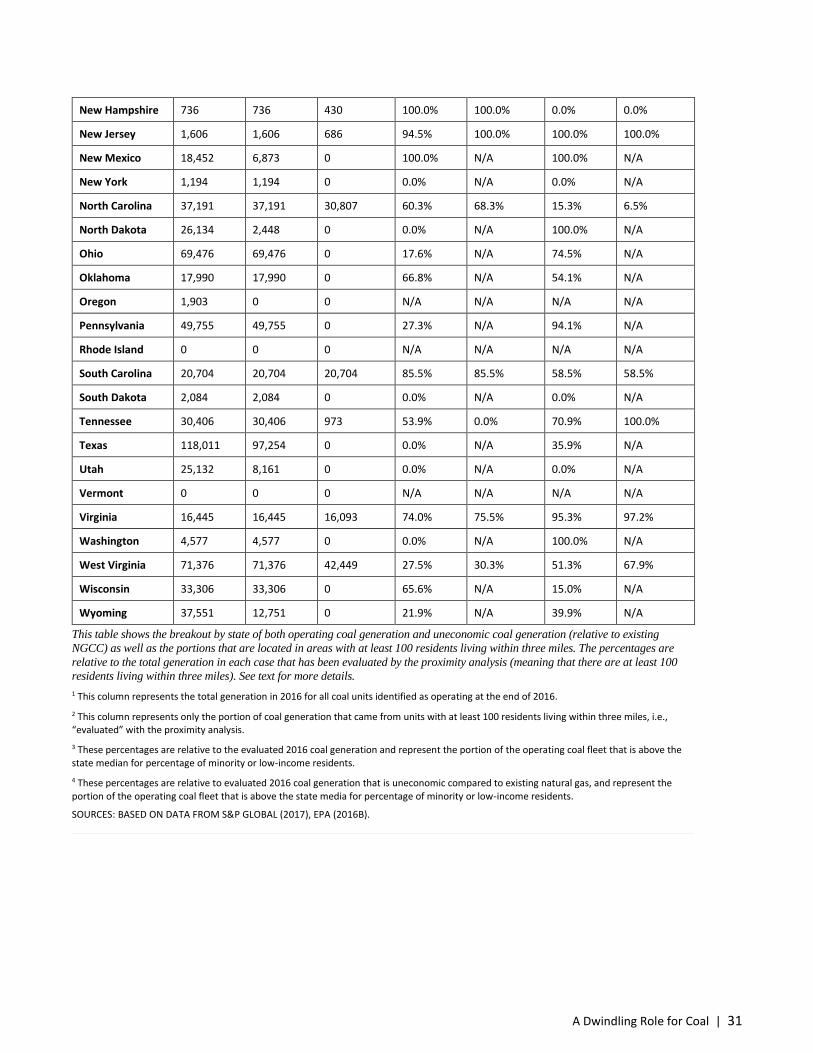
This table shows the breakout by state of both operating coal generation and uneconomic coal generation (relative to existing

NGCC) as well as the portions that are located in areas with at least 100 residents living within three miles. The percentages are

relative to the total generation in each case that has been evaluated by the proximity analysis (meaning that there are at least 100

residents living within three miles). See text for more details.

1 This column represents the total generation in 2016 for all coal units identified as operating at the end of 2016.

2 This column represents only the portion of coal generation that came from units with at least 100 residents living within three miles, i.e., “evaluated” with the proximity analysis.

3 These percentages are relative to the evaluated 2016 coal generation and represent the portion of the operating coal fleet that is above the state median for percentage of minority or low-income residents.

4 These percentages are relative to evaluated 2016 coal generation that is uneconomic compared to existing natural gas, and represent the portion of the operating coal fleet that is above the state media for percentage of minority or low-income residents.

SOURCES: BASED ON DATA FROM S&P GLOBAL (2017), EPA (2016B).


TABLE A14. Total Coal Capacity in GW by Region and Status

Region



Known or Possible

Conversion

Uneconomic Compared to

Existing NGCC

Remaining Economic

Units

Excluded from Stress

Test

RFC 86.9 26.0 4.8 12.4 2.3 14.6 56.0 1.6

SERC 86.1 19.5 5.7 9.5 1.7 35.0 39.4 0.5

TRE 20.1 0.2 - 0.9 - - 19.2 -

WECC 33.1 4.5 0.4 7.9 3.8 0.6 20.3 0.6

SPP 21.6 2.2 0.5 1.1 2.1 - 18.4 0.2

MRO 23.0 3.3 1.0 1.5 2.5 0.1 18.3 0.6

FRCC 9.7 0.3 0.3 2.7 - 6.4 0.3 0.3

NPCC 3.2 3.2 0.6 2.1 0.4 0.6 - 0.2

HI 0.2 0.0 - - - - - 0.2

ASCC 0.1 0.0 - - - - - 0.1

Similar to data in Table A7, future status is tabulated only for units that were operating at the end of 2016.

Key to NERC regions: ReliabilityFirst Corporation (RFC); Southeast Reliability Corporation (SERC); Texas Reliability Entity (TRE); Western Electricity Coordinating Council (WECC); Southwest Power Pool (SPP); Midwest Reliability Organization (MRO); Florida Reliability Coordinating Council (FRCC); and Northeast Power Coordinating Council (NPCC). Hawaii (HI) and Alaska Systems Coordinating Council (ASCC) are not NERC regions but are included for completeness.


TABLE A15. Net Generation from Coal in 2008 and 2016 in GWh by Region and Status

NERC Region



Known or Possible

Conversion

Uneconomic Compared to

Existing NGCC

Remaining Economic

Units

Excluded from Stress

Test

RFC 499,799 118,185 22,260 35,595 6,487 63,699 243,286 1

SERC 486,793 98,734 31,509 29,347 3,682 129,207 191,052 477

TRE 117,152 819 - 2,428 - - 94,740 -

WECC 209,620 16,659 2,250 33,888 16,914 2,532 110,471 -

SPP 117,655 13,659 2,542 3,331 6,843 - 85,642 83

MRO 136,130 12,776 3,675 3,681 10,005 243 96,025 431

FRCC 55,184 1,718 2,089 6,875 - 29,657 1,895 1,485

NPCC 22,588 12,151 3,801 3,099 182 430 - 847

HI 1,599 190 - - - - - 1,513

ASCC 398 - - - - - - 192

Similar to the data in Table A8, for current status, generation is tabulated for 2008; for future status, the values are 2016 generation (both in

GWh). Future status is tabulated only for units that are listed as operating in 2016.

Key to NERC regions: ReliabilityFirst Corporation (RFC); Southeast Reliability Corporation (SERC); Texas Reliability Entity (TRE); Western Electricity Coordinating Council (WECC); Southwest Power Pool (SPP); Midwest Reliability Organization (MRO); Florida Reliability Coordinating Council (FRCC); and Northeast Power Coordinating Council (NPCC). Hawaii (HI) and Alaska Systems Coordinating Council (ASCC) are not NERC regions but are included for completeness.


References

Cleetus, R., S. Clemmer, E. Davis, J. Deyette, J. Downing, and S. Frenkel. 2012. Ripe for retirement: The case for closing

America’s costliest coal plants. Cambridge, MA: Union of Concerned Scientists. Online at www.ucsusa.org/clean_energy/smart-

energy-solutions/decrease-coal/ripe-for-retirement-closing-americas-costliest-coal-plants.html, accessed June 22, 2017.

Chakraborty, J., J. Maantay, and J. Brender. 2011. Disproportionate proximity to environmental health hazards: Methods, models,

and measurement. American Journal of Public Health 101:S27–S36.

Declet-Bareto, J., et al. 2017. Energy and environmental justice communities: An exploratory analysis of power plant pollutant

burdens on environmental justice communities in northeastern states. Manuscript in preparation.

Deyette, J. 2015. The natural gas gamble: A risky bet on America's clean energy future. Cambridge, MA: Union of Concerned

Scientists. Online at http://www.ucsusa.org/sites/default/files/attach/2015/03/natural-gas-gamble-full-report.pdf, accessed June 22,

2017.

Energy Information Administration (EIA). 2017a. Annual energy outlook 2017. Washington, DC: Department of Energy. Online at

https://www.eia.gov/outlooks/aeo/, accessed 10 August 2017.

Energy Information Administration (EIA). 2017b. Electric power monthly: Table 6.7.A. Washington, DC: Department of Energy.

Online at https://www.eia.gov/electricity/monthly/epm_table_grapher.php?t=epmt_6_07_a, accessed June 22, 2017.

Energy Information Administration (EIA). 2016. Form EIA-860 detailed data. Washington, DC: Department of Energy. Online at

https://www.eia.gov/electricity/data/eia860/index.html, accessed June 22, 2017.

Eurek, K., et al. 2016. Regional energy deployment system (ReEDS) model documentation: Version 2016. Golden, CO: National

Renewable Energy Laboratory. Online at https://www.nrel.gov/docs/fy17osti/67067.pdf, accessed 10 August 2017.

Fisher, J., and B. Biewald. 2011. Environmental controls and the WECC coal fleet: Estimating the forward-going economic merit of

coal-fired power plants in the West with new environmental controls. Cambridge, MA: Synapse Energy Economics. Online at

http://www.synapse-energy.com/sites/default/files/SynapseReport.2011-01.EF%2BWGG.WGG-Coal-Plant-Database.10-077-

Report_0.pdf, accessed 10 August 2017.

Fleischman, L., R. Cleetus, S. Clemmer, J. Deyette, and S. Frenkel. 2013. Ripe for retirement: An economic analysis of the US coal

fleet. Cambridge, MA: Union of Concerned Scientists. Online at www.ucsusa.org/clean_energy/smart-energy-solutions/decrease-

coal/economic-analysis-us-coal-plants.html, accessed June 22, 2017.

Hand, M., et al. 2016. 2016 annual technology baseline. Golden, CO: National Renewable Energy Laboratory. Online at

https://data.nrel.gov/submissions/52, accessed August 10, 2017.

Interagency Working Group on the Social Cost of Greenhouse Gases. 2016. Technical support document: Technical update of the

social cost of carbon for regulatory impact analysis under Executive Order 12866. Washington, DC: United States Government.

Archived at https://obamawhitehouse.archives.gov/sites/default/files/omb/inforeg/scc_tsd_final_clean_8_26_16.pdf, accessed June

22, 2017.

Krieger, E., A. McPhail, E. Czolowski, J. Hays, and S.B.C. Shonkoff. 2016. The Clean Power Plan in Pennsylvania and Ohio:

Analyzing power generation for health and equity. Oakland, CA: PSE Healthy Energy. Online at www.psehealthyenergy.org/our-

work/publications/archive/our-air-health-and-equity-impacts-of-ohios-power-plants/, accessed 22 June 2017.


Kruger, J. 2017. Hedging an uncertain future: Internal carbon prices in the electric power sector. Washington, DC: Resources for

the Future. Online at http://www.rff.org/files/document/file/RFF-Rpt-Kruger-Internal%20Carbon%20Pricing.pdf, accessed August

10, 2017.

Lawrence Berkeley National Laboratory (LBNL). 2017. RPS compliance data. Berkeley, CA. Online at

https://emp.lbl.gov/projects/renewables-portfolio, accessed July 28, 2017.

North American Electric Reliability Corporation (NERC). 2016. 2016 long-term reliability assessment. Atlanta, GA. Online at

http://www.nerc.com/pa/RAPA/ra/Reliability%20Assessments%20DL/2016%20Long-Term%20Reliability%20Assessment.pdf,

accessed June 22, 2017.

North American Electric Reliability Corporation (NERC). 2010. Special reliability scenario assessment: Resource adequacy

impacts of potential US environmental regulations. Princeton, NJ. Online at http://www.nerc.om/files/EPA_Scenario_Final.pdf,

accessed August 24, 2017.

S&P Global Market Intelligence (S&P Global). 2017. SNL interactive. New York. Online at www.snl.com (paywall restricted),

accessed June 22, 2017.

Synapse Energy Economics. 2015. Synapse’s coal asset valuation tool. Cambridge, MA. Online at http://www.synapse-

energy.com/project/synapses-coal-asset-valuation-tool, accessed July 20, 2017.

US Environmental Protection Agency (EPA). 2016a. National electric energy data system v.5.15. Washington, DC. Online at

https://www.epa.gov/airmarkets/needs-v515-user-guide, accessed August 10, 2017.

US Environmental Protection Agency (EPA). 2016b. EJSCREEN geodatabase, V3, USPR 090216. Washington, DC. Online at

ftp://newftp.epa.gov/EJSCREEN/2016/EJSCREEN_V3_USPR_090216.gdb.zip, downloaded May 11, 2017.

US Environmental Protection Agency (EPA). 2016c. EJSCREEN environmental justice mapping and screening tool: Technical

documentation—Draft. Washington, DC: Office of Policy. Online at

ftp://newftp.epa.gov/EJSCREEN/2016/EJSCREEN_Technical_Document_20160704_DRAFT.pdf, accessed June 22, 2017.

US Environmental Protection Agency (EPA). 2016d. EJSCREENBatch. Washington, DC. Shared via agency May 17, 2017.

US Environmental Protection Agency (EPA). 2015. EJ screening report for the Clean Power Plan. Research Triangle Park, NC:

Office of Air and Radiation. Online at archive.epa.gov/epa/cleanpowerplan/ej-screening-report-clean-power-plan.html, accessed

22 June 22, 2017.

US Environmental Protection Agency (EPA). 2014. Background and draft methodology for estimating energy impacts of EE/RE

policies. Washington, DC. Archived at https://archive.epa.gov/epa/sites/production/files/2015-

08/documents/epa_background_and_methodology_ee_re_02122014.pdf, accessed August 29, 2017.

US Environmental Protection Agency (EPA). 2013. Technical support document: Estimating the benefit per ton of reducing PM2.5

precursors from 17 sectors. Research Triangle Park, NC: Office of Air and Radiation. Online at

https://www.epa.gov/sites/production/files/2014-10/documents/sourceapportionmentbpttsd.pdf, accessed June 22, 2017.

Wilson, A., J. Patterson, K. Wasserman, A. Starbuck, A. Sartor, J. Hatcher, J. Fleming, and K. Fink. 2012. Coal blooded: Putting

profits before people. Baltimore, MD: National Association for the Advancement of Colored People. Online at

http://www.naacp.org/climate-justice-resources/coal-blooded/, accessed August 29, 2017.

https://www.epa.gov/airmarkets/needs-v515-user-guide

A Dwindling Role for Coal - Union of Concerned … Dwindling Role for Coal | 1 This document details...

Documents

Transcript of A Dwindling Role for Coal - Union of Concerned … Dwindling Role for Coal | 1 This document details...