A Durbin-Watson serial correlation test for ARX processes via ...
15
HAL Id: hal-01023598 https://hal.archives-ouvertes.fr/hal-01023598 Submitted on 14 Jul 2014 HAL is a multi-disciplinary open access archive for the deposit and dissemination of sci- entific research documents, whether they are pub- lished or not. The documents may come from teaching and research institutions in France or abroad, or from public or private research centers. L’archive ouverte pluridisciplinaire HAL, est destinée au dépôt et à la diffusion de documents scientifiques de niveau recherche, publiés ou non, émanant des établissements d’enseignement et de recherche français ou étrangers, des laboratoires publics ou privés. A Durbin-Watson serial correlation test for ARX processes via excited adaptive tracking Bernard Bercu, Bruno Portier, Victor Vazquez To cite this version: Bernard Bercu, Bruno Portier, Victor Vazquez. A Durbin-Watson serial correlation test for ARX processes via excited adaptive tracking. 2014. <hal-01023598>
Transcript of A Durbin-Watson serial correlation test for ARX processes via ...

HAL Id: hal-01023598https://hal.archives-ouvertes.fr/hal-01023598
Submitted on 14 Jul 2014
HAL is a multi-disciplinary open accessarchive for the deposit and dissemination of sci-entific research documents, whether they are pub-lished or not. The documents may come fromteaching and research institutions in France orabroad, or from public or private research centers.
L’archive ouverte pluridisciplinaire HAL, estdestinée au dépôt et à la diffusion de documentsscientifiques de niveau recherche, publiés ou non,émanant des établissements d’enseignement et derecherche français ou étrangers, des laboratoirespublics ou privés.
A Durbin-Watson serial correlation test for ARXprocesses via excited adaptive tracking
Bernard Bercu, Bruno Portier, Victor Vazquez
To cite this version:Bernard Bercu, Bruno Portier, Victor Vazquez. A Durbin-Watson serial correlation test for ARXprocesses via excited adaptive tracking. 2014. <hal-01023598>

A DURBIN-WATSON SERIAL CORRELATION TEST FOR ARX
PROCESSES VIA EXCITED ADAPTIVE TRACKING
BERNARD BERCU, BRUNO PORTIER, AND VICTOR VAZQUEZ
Abstract. We propose a new statistical test for the residual autocorrelation in ARXadaptive tracking. The introduction of a persistent excitation in the adaptive track-ing control allows us to build a bilateral statistical test based on the well-knownDurbin-Watson statistic. We establish the almost sure convergence and the asymp-totic normality for the Durbin-Watson statistic leading to a powerful serial correlationtest. Numerical experiments illustrate the good performances of our statistical testprocedure.
1. Introduction
Model validation is an important and essential final step in the identification of sto-chastic dynamical systems. This validation step is often done through the analysisof residuals of the model considered. In particular, testing the non-correlation of theresiduals is a crucial task since many theoretical results require independence of thedriven noise of the systems. Moreover, non-compliance with this hypothesis can leadto misinterpretation of the theoretical results. For example, it is well known that forlinear autoregressive models with autocorrelated residuals, the least squares estimator isasymptotically biased, see e.g. [5], [11], [14], [15], and therefore the estimated modelis not the correct one. Consequently, to ensure a good interpretation of the results,it is necessary to have a powerful tool allowing to detect the possible autocorrelationof the residuals. The well-known statistical test of Durbin-Watson was introduced todeal with this question, and more specifically, for detecting the presence of a first-orderautocorrelated noise in linear regression models [8], [9], [10], [11], firstly and for linearautoregressive models [5], [14], [16], [17], [15], secondly.
To the best of our knowledge, no such serial correlation statistical test is availablefor controlled autoregressive processes. The aim of this paper is to carry out a serialcorrelation test, based on the Durbin-Watson statistic, for the ARX(p, 1) process given,for all n ≥ 0, by
(1.1) Xn+1 =
p∑
k=1
θkXn−k+1 + Un + εn+1
where the driven noise (εn) is given by the first-order autoregressive process
(1.2) εn+1 = ρ εn + Vn+1
and the control objective is the tracking of a given reference trajectory. More precisely,we shall propose a bilateral statistical test allowing to decide between the null hypothesis
2000Mathematics Subject Classification. Primary: 62G05 Secondary: 93C40, 62F05, 60F15, 60F05.Key words and phrases. Durbin-Watson statistic, Estimation, Adaptive tracking control, Persistent
excitation, Almost sure convergence, Asymptotic normality, Statistical test for serial autocorrelation.1

2 BERNARD BERCU, BRUNO PORTIER, AND VICTOR VAZQUEZ
H0 : 〈〈ρ = 0 〉〉 which ensures that the driven noise is not correlated, and the alternativeone H1 : 〈〈ρ 6= 0 〉〉 which means that the residual process is effectively first-order auto-correlated. The choice of the Durbin-Watson statistic, instead of any other statisticaltests, is governed by its efficienty for autoregressive processes without control, see [5],[11], [14], [15].
In contrast with the recent work [6], we propose to make use of a different strategy viaa modification of the adaptive control law. This modification relies on the introductionof an additional persistent excitation. Since the pioneering works of Anderson [1] andMoore [13], the concept of persistent excitation has been successfully developped inmany fields of applied mathematics such as identification of complex systems, feedbackadaptive control, etc. While it was not possible in [6] to test the non correlation of thedriven noise (εn), that is to test whether or not ρ = 0, the introduction of an additionalpersistent excitation term in the control law will be the key point to build our serialcorrelation test. Moreover, we wish to mention that all previous works devoted to noncorrelation test based on the Durbin-Watson statistic were only related to uncontrolledprocesses. Therefore, thanks to the persistent excitation, our statistical test is at ourknowledge the first one in the context of linear processes with adaptive control.
The paper is organized as follows. Section 2 is devoted to the ARX process and tothe persistently excited adaptive control law. In Section 3, we establish the asymptoticproperties of the Durbin-Watson statistic as well as a bilateral statistical test for residualautocorrelation. Some numerical experiments are provided in Section 4. Finally, alltechnical proofs are postponed in the Appendices.
2. Model and excited adaptive tracking
We focus our attention on the ARX(p, 1) process given, for all n ≥ 0, by
(2.1) Xn+1 =
p∑
k=1
θkXn−k+1 + Un + εn+1
where the driven noise (εn) is given by the first-order autoregressive process
(2.2) εn+1 = ρ εn + Vn+1.
We assume that the autocorrelation parameter satisfies |ρ| < 1 and the initial valuesX0, ε0 and U0 may be arbitrarily chosen. We also assume that (Vn) is a martingaledifference sequence adapted to the filtration F = (Fn) where Fn is the σ-algebra of theevents occurring up to time n, such that, for all n ≥ 0, E
[V 2n+1|Fn
]= σ2 a.s. with
σ2 > 0. We denote by θ the unknown parameter of the ARX(p, 1) process,
θt = (θ1, . . . , θp).
Our control strategy is to regulate the dynamic of the process (Xn) by forcing Xn totrack a bounded reference trajectory (xn). We assume that (xn) is predictable whichmeans that for all n ≥ 1, xn is Fn−1-measurable. For the sake of simplicity, we alsoassume that
(2.3)
n∑
k=1
x2k = o(n) a.s.

A DURBIN-WATSON SERIAL CORRELATION TEST FOR ARX PROCESSES 3
In order to regulate the dynamic of the process (Xn) given by (2.1), we propose tomake use of the adaptive control law introduced in [6] together with additional persistentexcitation. The strategy consists of using a control associated with a higher order modelthan the initial ARX(p, 1), and more precisely an ARX(p+1, 2) model. The introductionof an additional excitation in the control law will be the key point to build our serialcorrelation test for the driven noise (εn), that is to test wether or not ρ = 0. Denote by(ξn) a centered exogenous noise with known variance ν2 > 0, which will play the role ofthe additional excitation. We assume that (ξn) is independent of (Vn), of (xn) and ofthe initial state of the system. One can observe that these assumptions are not at allrestrictive as we have in our own hands the additional excitation (ξn)
The excited adaptive control law is given, for all n ≥ 0, by
(2.4) Un = xn+1 − ϑ tn Φn + ξn+1
where ϑn stands for the least squares estimator of the unknown parameter of the ARX(p+1, 2) model with uncorrelated driven noise
(2.5) Xn+1 = ϑtΦn + Un + Vn+1
where the new parameter ϑ ∈ Rp+2 is related to θ and ρ by the identity
(2.6) ϑ =
θ00
− ρ
−1θ1
and the new regression vector is given by
Φtn = (Xn, . . . , Xn−p, Un−1).
It is well-known that ϑn satisfies the recursive relation
(2.7) ϑn+1 = ϑn + S−1n Φn
(Xn+1 − Un − ϑ t
nΦn
)
where the initial value ϑ0 may be arbitrarily chosen and
(2.8) Sn =n∑
k=0
ΦkΦtk + Ip+2.
As usual, the identity matrix Ip+2 is added in order to avoid useless invertibility assump-tion. One can immediately see from (2.6) that the last component of the vector ϑ is−ρ. Consequently, we obtain an estimator of ρ by simply taking the opposite of the last
coordinate of ϑn which will be denoted by ρn. In addition, one can also deduce from(2.6) that
(2.9)
(θρ
)= ∆ϑ

4 BERNARD BERCU, BRUNO PORTIER, AND VICTOR VAZQUEZ
where ∆ is the rectangular matrix of size (p+ 1)×(p+ 2) given by
(2.10) ∆ =
1 0 · · · · · · · · · 0 1ρ 1 0 · · · · · · 0 ρρ2 ρ 1 0 · · · 0 ρ2
· · · · · · · · · · · · · · · · · · · · ·ρp−1 ρp−2 · · · ρ 1 0 ρp−1
0 0 · · · · · · · · · 0 −1
.
Then, starting from (2.9) and replacing ρ by ρn in (2.10), we can estimate θ by
(2.11) θn =(Ip 0
)∆n ϑn
where ϑn is given by (2.7) and
(2.12) ∆n =
1 0 · · · · · · · · · 0 1ρn 1 0 · · · · · · 0 ρnρ 2n ρn 1 0 · · · 0 ρ 2
n
· · · · · · · · · · · · · · · · · · · · ·ρ p−1n ρ p−2
n · · · ρn 1 0 ρ p−1n
0 0 · · · · · · · · · 0 −1
.
From the almost sure convergence of ϑn to ϑ, we easily deduce the almost sure conver-
gences of θn and ρn to θ and ρ, respectively.
3. A Durbin-Watson serial correlation test
We are in the position to introduce our serial correlation test based on the Durbin-Watson statistic which is certainly the most commonly used statistics for testing thepresence of serial autocorrelation. Our goal is to test
H0 : 〈〈ρ = 0 〉〉 vs H1 : 〈〈ρ 6= 0 〉〉.
For that purpose, we consider the Durbin-Watson statistic [5], [8], [9], [10], [11] given,for all n ≥ 1, by
(3.1) Dn =
∑n
k=1 (εk − εk−1)2
∑n
k=0 ε2k
where the residuals εk are defined, for all 0 ≤ k ≤ n, by
(3.2) εk = Xk − Uk−1 − θ tnϕk−1
with θn given by (2.11) and ϕtn = (Xn, . . . , Xn−p+1). The initial value ε0 may be
arbitrarily chosen and we take ε0 = X0.
On the one hand, we would like to emphasize that it is not possible to perform thisstatistical test if the control law is not persistently excited [6]. On the other hand, onecan notice that it is also possible to estimate the serial correlation parameter ρ by theleast squares estimator
(3.3) ρn =
∑n
k=1 εkεk−1∑n
k=1 ε2k−1

A DURBIN-WATSON SERIAL CORRELATION TEST FOR ARX PROCESSES 5
which is certainly the more natural estimator of ρ. The Durbin-Watson statistic Dn isrelated to ρn by the linear relation
(3.4) Dn = 2(1− ρn) + ζn
where the remainder ζn plays a negligeable role. The almost sure properties of Dn andρn are as follows.
Theorem 3.1. Assume (Vn) has a finite conditional moment of order > 2. Then, ρnconverges almost surely to ρ
(3.5) (ρn − ρ)2 = O(logn
n
)a.s.
In addition, Dn converges almost surely to D = 2(1− ρ). Moreover, if (Vn) has a finite
conditional moment of order > 4, we also have
(3.6)(Dn −D
)2= O
(log n
n
)a.s.
Proof. The proofs are given in Appendix A.
Let us now give the asymptotic normality of the Durbin-Watson statistic which will beuseful to build our serial correlation test.
Theorem 3.2. Assume that (Vn) has finite conditional moments of order > 2. Then,
we have
(3.7)√n(ρn − ρ)
L−→ N(0, τ 2
)
where the asymptotic variance τ 2 is given by
τ 2 =(1− ρ2)
(σ2 + ν2)(ν2 + σ2ρ2(p+1))
[((σ2 − ν2)− (p+ 1)σ2ρ2p + (p− 1)σ2ρ2(p+1)
)2
+ σ2(ν2 + σ2ρ2(p+1))(4− (4p+ 3)ρ2p + 4pρ2(p+1) − ρ2(2p+1)
)].(3.8)
Moreover, if (Vn) has finite conditional moments of order > 4, we also have
(3.9)√n(Dn −D)
L−→ N(0, 4τ 2
).
Proof. The proofs are given in Appendix B.
Remark 3.1. We now point out the crucial role played by the additional excitationin the control law given by (2.4). It follows from (3.8) that if ρ = 0, then τ 2 reducesto
τ 2 =σ2 + ν2
ν2.
Consequently, if ν2 = 0 i.e. there is no persistent excitation, then this varianceexplodes. Therefore, the persistent excitation allows to investigate the importantcase ρ = 0 and more generally to stabilize the asymptotic variance of the Durbin-Watson statistic.
6 BERNARD BERCU, BRUNO PORTIER, AND VICTOR VAZQUEZ
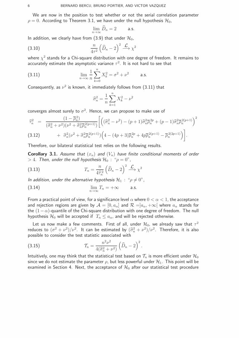
We are now in the position to test whether or not the serial correlation parameterρ = 0. According to Theorem 3.1, we have under the null hypothesis H0,
limn→∞
Dn = 2 a.s.
In addition, we clearly have from (3.9) that under H0,
(3.10)n
4τ 2
(Dn − 2
)2 L−→ χ2
where χ2 stands for a Chi-square distribution with one degree of freedom. It remains toaccurately estimate the asymptotic variance τ 2. It is not hard to see that
(3.11) limn→∞
1
n
n∑
k=0
X2k = σ2 + ν2 a.s.
Consequently, as ν2 is known, it immediately follows from (3.11) that
σ2n =
1
n
n∑
k=1
X2k − ν2
converges almost surely to σ2. Hence, we can propose to make use of
τ 2n =(1− ρ 2
n)
(σ2n + ν2)(ν2 + σ2
nρ2(p+1)n )
[((σ2
n − ν2)− (p+ 1)σ2nρ
2pn + (p− 1)σ2
nρ2(p+1)n
)2
+ σ2n(ν
2 + σ2nρ
2(p+1)n )
(4− (4p+ 3)ρ 2p
n + 4pρ 2(p+1)n − ρ 2(2p+1)
n
)].(3.12)
Therefore, our bilateral statistical test relies on the following results.
Corollary 3.1. Assume that (xn) and (Vn) have finite conditional moments of order
> 4. Then, under the null hypothesis H0 : “ρ = 0”,
(3.13) Tn =n
4τ 2n
(Dn − 2
)2 L−→ χ2
In addition, under the alternative hypothesis H1 : “ρ 6= 0”,
(3.14) limn→∞
Tn = +∞ a.s.
From a practical point of view, for a significance level α where 0 < α < 1, the acceptanceand rejection regions are given by A = [0, aα] and R =]aα,+∞[ where aα stands forthe (1−α)-quantile of the Chi-square distribution with one degree of freedom. The nullhypothesis H0 will be accepted if Tn ≤ aα, and will be rejected otherwise.
Let us now make a few comments. First of all, under H0, we already saw that τ 2
reduces to (σ2 + ν2)/ν2. It can be estimated by (σ2n + ν2)/ν2. Therefore, it is also
possible to consider the test statistic associated with
(3.15) Tn =n2ν2
4(σ2n + ν2)
(Dn − 2
)2.
Intuitively, one may think that the statistical test based on Tn is more efficient under H0
since we do not estimate the parameter ρ, but less powerful under H1. This point will beexamined in Section 4. Next, the acceptance of H0 after our statistical test procedure

A DURBIN-WATSON SERIAL CORRELATION TEST FOR ARX PROCESSES 7
should lead to a change of control law. As a matter of fact, if we accept ρ = 0, thedriven noise (εn) is not correlated. It means that we can implement the usual controllaw [2] associated with model (2.1) given, for all n ≥ 0, by
Un = xn+1 − θ tnϕn
where θn stands for the standard least-squares estimator associated with (2.1). Finally,the test provided by Corollary 3.1 may be of course extended if we replace zero by anyρ0 ∈ R with |ρ0| < 1 in the null hypothesis. To be more precise, we are able as in [6]to test H0 : 〈〈ρ = ρ0 〉〉 versus H1 : 〈〈ρ 6= ρ0 〉〉. We wish to mention that the asymptoticvariance τ 2 is smaller than the one obtained in [6].
4. Numerical Experiments
This section is devoted to the application of our Durbin-Watson serial correlationtest. Although this test has several potential of being applied in concrete situations, alarge search in the literature did not offer any one. We then consider artificial modelsfor illustrative purposes and for studying the empirical level and power of our test forsample sizes from small to moderate, that is n = 50, 100, 200, 500, 1000 and 2000.
In order to keep this section brief, we restrict ourself to the three explosive models inopen-loop
Xn+1 =3
2Xn + Un + εn+1(4.1)
Xn+1 = −Xn + 2Xn−1 + Un + εn+1(4.2)
Xn+1 = Xn +1
2Xn−1 +
1
4Xn−2 + Un + εn+1(4.3)
where the driven noise (εn) is given by (2.2) and (Vn) is a sequence of independent andidentically distributed random variables with N (0, 1) distribution. The control law Un isgiven by (2.4) where, for the sake of simplicity, the reference trajectory xn = 0 and thepersistent excitation (ξn) s a sequence of independent and identically distributed randomvariables with N (0, ν2) distribution.
For each model, we based our numerical simulations on N = 1000 realizations ofsample size n. We use a short learning period of 100 time steps. This learning periodallows us to forget the transitory phase. The level of significance is set to α = 5%. Forthe statistical tests based on Tn and Tn, we are interested in the empirical level underH0 to be compared to the theoretical level 5%, and the empirical power under H1, tobe compared with 1.
First of all, let us study the effect of the variance ν2 of the exogenous noise (ξn) onthe behavior of the statistical test under H0.

8 BERNARD BERCU, BRUNO PORTIER, AND VICTOR VAZQUEZ
n 50 100 200 500 1000 2000
ν = 0.5 Tn 0.9% 1.6% 2% 3% 2.9% 4.9%Tn 0% 0.1% 0.5% 2.1% 2.4% 4.4%
ν = 1 Tn 2.5% 2.5% 3.3% 4.4% 4.4% 4.9%Tn 1.3% 1.3% 2.5% 4.1% 4% 4.8%
ν = 2 Tn 5.2% 4.1% 4.9% 5.3% 4.7% 4.6%Tn 3.7% 3.7% 4.1% 5.1% 4.7% 4.6%
ν = 3 Tn 5.8% 5.1% 5.6% 4.3% 4.3% 4.8%Tn 4.5% 4.6% 5.1% 4.2% 4.3% 4.7%
Table 1. Model (4.1). Percentage of rejections of our test under H0
(to be compared to the 5% theoretical level).
It is clear from Table 1, where one can find the results obtained for different values ofν, that the variance of the persistent excitation (ξn) in the control law plays a crucialrole. Indeed, one can observe that if it is too small, then the empirical level of the testis bad for sample sizes from small to moderate n ≤ 1000. Of course, a high value of ν2
improves the performance of the test under H0, but degrades the performance of thetracking. The value ν = 2 realizes a good compromise and allows a good calibration ofthe test under H0.
n 50 100 200 500 1000 2000Model (4.1) Tn 5.2% 4.1% 4.9% 5.3% 4.7% 4.6%
Tn 3.7% 3.7% 4.1% 5.1% 4.7% 4.6%Model (4.2) Tn 5.9% 3% 3.9% 4.6% 4.8% 5.2%
Tn 4.7% 2.5% 3.7% 4.5% 4.8% 5.1%Model (4.3) Tn 4.8% 4.7% 4.1% 5.2% 4.9% 6%
Tn 3.8% 3.5% 3.9% 5% 4.9% 5.9%
Table 2. Percentage of rejections of our test under H0 (to be comparedto the 5% theoretical level). ν = 2.
One can find in Table 2 the percentage of rejections of our test under H0 for thethree different models (4.1) to (4.3). The empirical levels of the test are close to the 5%theoretical level even for small sample sizes. Both statistical tests based on Tn and Tn
are comparable even if the test statistic Tn systematically tends to less reject H0 thanthe test statistic Tn.
Let us now study the empirical power of our statistical test. One can find in Tables 3to 5 the results obtained for each of the three models (4.1) to (4.3). As expected, it isdifficult to reject H0 when ρ = 0.05 for small sample sizes or ρ = 0.1 to a lesser extent.However, the test performs pretty well as the percentage of correct decisions increaseswith the sample size.

A DURBIN-WATSON SERIAL CORRELATION TEST FOR ARX PROCESSES 9
n 50 100 200 500 1000 2000
ρ = 0.05 Tn 6.4% 7.1% 9.6% 18.8% 30.6% 50.3%Tn 4.8% 6.2% 9% 18.4% 30.5% 50.2%
ρ = 0.1 Tn 11.1% 17.4% 25.9% 56.8% 81.9% 98.2%Tn 8.9% 15.2% 24.7% 56.2% 81.6% 98.1%
ρ = 0.2 Tn 32% 47.5% 77.6% 98.9% 100% 100%Tn 10.7% 24.1% 49.5% 91.2% 99.5% 100%
ρ = 0.3 Tn 57% 83% 97.7% 100% 100% 100%Tn 51.7% 81.7% 97.5% 100% 100% 100%
ρ = 0.4 Tn 78.8% 97.2% 99.7% 100% 100% 100%Tn 73.4% 96.5% 99.7% 100% 100% 100%
Table 3. Model (4.1). Percentage of correct decisions of our test under H1.
We further observe, as expected, that for a fixed value of the sample size n, thehigher the value of ρ is, the more the percentage of correct decisions increases. We alsonotice that for a fixed value of ρ, the empirical power increases with the sample size. Inconclusion, the test performs very well under H1. Moreover, higher values of the orderp does not degrade the performances of our statistical test.
n 50 100 200 500 1000 2000
ρ = 0.05 Tn 5.2% 6.2% 11% 17.6% 28.5% 54.6%Tn 4.5% 5.6% 10.7% 17.4% 28.3% 54.6%
ρ = 0.1 Tn 11.5% 15% 25.3% 53% 78.1% 97.3%Tn 9.7% 14.1% 24.6% 52.5% 78.1% 97.3%
ρ = 0.2 Tn 28.5% 45.8% 70.9% 98.3% 99.9% 100%Tn 24.4% 44.1% 69.6% 98.3% 99.9% 100%
ρ = 0.3 Tn 53.1% 80.6% 97% 100% 100% 100%Tn 48.4% 79.1% 96.9% 100% 100% 100%
ρ = 0.4 Tn 77.4% 96.4% 100% 100% 100% 100%Tn 74% 95.9% 100% 100% 100% 100%
Table 4. Model (4.2). Percentage of correct decisions of our test under H1.
Finally, one can realize that for small sample sizes, the statistical test based on Tn
is less powerful than the one associated with Tn. We also wish to mention that, bysymmetry, the performance of our statistical tests are the same for negative values of ρ.
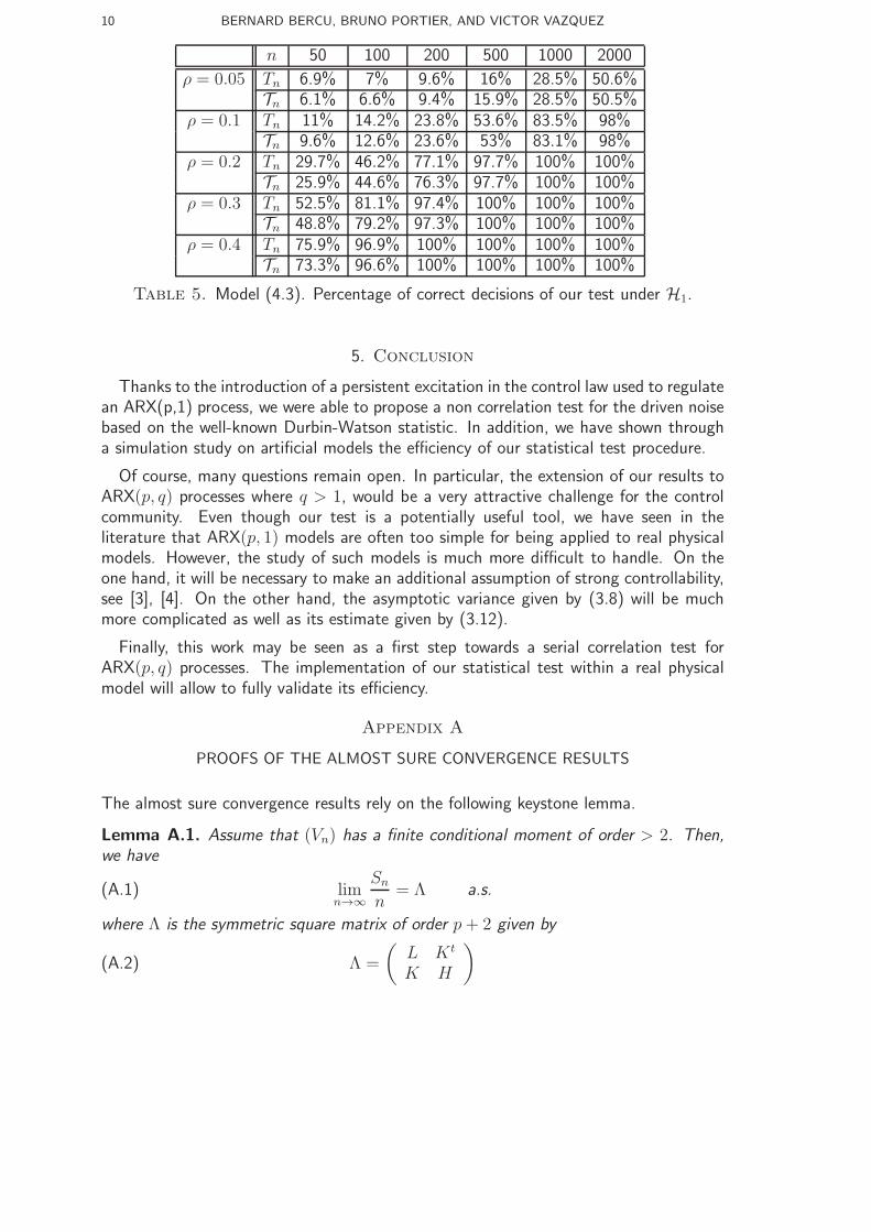
10 BERNARD BERCU, BRUNO PORTIER, AND VICTOR VAZQUEZ
n 50 100 200 500 1000 2000
ρ = 0.05 Tn 6.9% 7% 9.6% 16% 28.5% 50.6%Tn 6.1% 6.6% 9.4% 15.9% 28.5% 50.5%
ρ = 0.1 Tn 11% 14.2% 23.8% 53.6% 83.5% 98%Tn 9.6% 12.6% 23.6% 53% 83.1% 98%
ρ = 0.2 Tn 29.7% 46.2% 77.1% 97.7% 100% 100%Tn 25.9% 44.6% 76.3% 97.7% 100% 100%
ρ = 0.3 Tn 52.5% 81.1% 97.4% 100% 100% 100%Tn 48.8% 79.2% 97.3% 100% 100% 100%
ρ = 0.4 Tn 75.9% 96.9% 100% 100% 100% 100%Tn 73.3% 96.6% 100% 100% 100% 100%
Table 5. Model (4.3). Percentage of correct decisions of our test under H1.
5. Conclusion
Thanks to the introduction of a persistent excitation in the control law used to regulatean ARX(p,1) process, we were able to propose a non correlation test for the driven noisebased on the well-known Durbin-Watson statistic. In addition, we have shown througha simulation study on artificial models the efficiency of our statistical test procedure.
Of course, many questions remain open. In particular, the extension of our results toARX(p, q) processes where q > 1, would be a very attractive challenge for the controlcommunity. Even though our test is a potentially useful tool, we have seen in theliterature that ARX(p, 1) models are often too simple for being applied to real physicalmodels. However, the study of such models is much more difficult to handle. On theone hand, it will be necessary to make an additional assumption of strong controllability,see [3], [4]. On the other hand, the asymptotic variance given by (3.8) will be muchmore complicated as well as its estimate given by (3.12).
Finally, this work may be seen as a first step towards a serial correlation test forARX(p, q) processes. The implementation of our statistical test within a real physicalmodel will allow to fully validate its efficiency.
Appendix A
PROOFS OF THE ALMOST SURE CONVERGENCE RESULTS
The almost sure convergence results rely on the following keystone lemma.
Lemma A.1. Assume that (Vn) has a finite conditional moment of order > 2. Then,
we have
(A.1) limn→∞
Sn
n= Λ a.s.
where Λ is the symmetric square matrix of order p+ 2 given by
(A.2) Λ =
(L Kt
K H
)
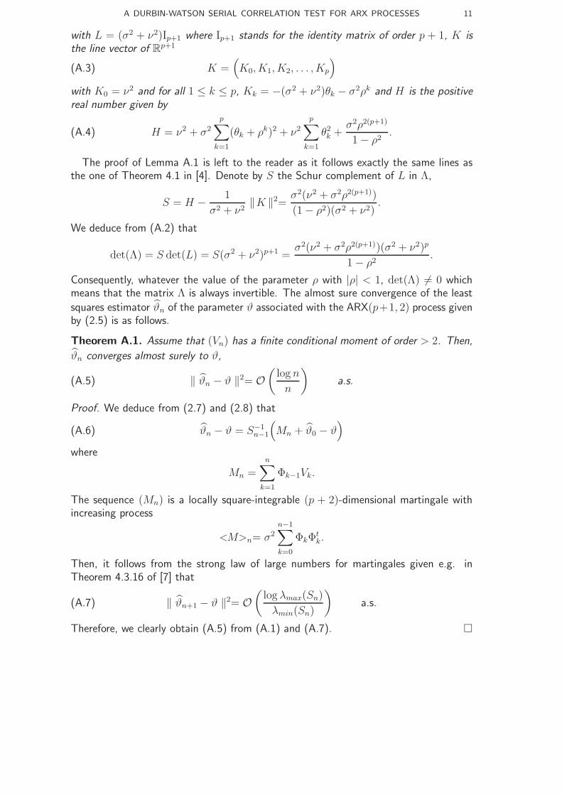
A DURBIN-WATSON SERIAL CORRELATION TEST FOR ARX PROCESSES 11
with L = (σ2 + ν2)Ip+1 where Ip+1 stands for the identity matrix of order p + 1, K is
the line vector of Rp+1
(A.3) K =(K0, K1, K2, . . . , Kp
)
with K0 = ν2 and for all 1 ≤ k ≤ p, Kk = −(σ2 + ν2)θk − σ2ρk and H is the positive
real number given by
(A.4) H = ν2 + σ2
p∑
k=1
(θk + ρk)2 + ν2
p∑
k=1
θ2k +σ2ρ2(p+1)
1− ρ2.
The proof of Lemma A.1 is left to the reader as it follows exactly the same lines asthe one of Theorem 4.1 in [4]. Denote by S the Schur complement of L in Λ,
S = H − 1
σ2 + ν2‖K ‖2= σ2(ν2 + σ2ρ2(p+1))
(1− ρ2)(σ2 + ν2).
We deduce from (A.2) that
det(Λ) = S det(L) = S(σ2 + ν2)p+1 =σ2(ν2 + σ2ρ2(p+1))(σ2 + ν2)p
1− ρ2.
Consequently, whatever the value of the parameter ρ with |ρ| < 1, det(Λ) 6= 0 whichmeans that the matrix Λ is always invertible. The almost sure convergence of the least
squares estimator ϑn of the parameter ϑ associated with the ARX(p+1, 2) process givenby (2.5) is as follows.
Theorem A.1. Assume that (Vn) has a finite conditional moment of order > 2. Then,
ϑn converges almost surely to ϑ,
(A.5) ‖ ϑn − ϑ ‖2= O(log n
n
)a.s.
Proof. We deduce from (2.7) and (2.8) that
(A.6) ϑn − ϑ = S−1n−1
(Mn + ϑ0 − ϑ
)
where
Mn =n∑
k=1
Φk−1Vk.
The sequence (Mn) is a locally square-integrable (p + 2)-dimensional martingale withincreasing process
<M>n= σ2n−1∑
k=0
ΦkΦtk.
Then, it follows from the strong law of large numbers for martingales given e.g. inTheorem 4.3.16 of [7] that
(A.7) ‖ ϑn+1 − ϑ ‖2= O(log λmax(Sn)
λmin(Sn)
)a.s.
Therefore, we clearly obtain (A.5) from (A.1) and (A.7). �

12 BERNARD BERCU, BRUNO PORTIER, AND VICTOR VAZQUEZ
We immediately deduce from Theorem A.1 the almost sure convergence of the least
squares estimators θn and ρn to θ and ρ.
Corollary A.1. Assume that (Vn) has a finite conditional moment of order > 2. Then,
θn and ρn both converge almost surely to θ and ρ,
(A.8) ‖ θn − θ ‖2= O(logn
n
)a.s.
(A.9) (ρn − ρ)2 = O(log n
n
)a.s.
Proof of Theorem 3.1. The proof of Theorem 3.1 relies on Corollary A.1. It is leftto the reader inasmuch as it follows essentially the same lines as those in Appendix C of[6].
Appendix B
PROOFS OF THE ASYMPTOTIC NORMALITY RESULTS
We shall now prove Theorem 3.2. First of all, we obtain from (3.3) that
(B.1) ρn =In
Jn−1
where
In =n∑
k=1
εkεk−1 and Jn =n∑
k=0
ε 2k .
As in [6], we deduce from (A.6) and (B.1) the martingale decomposition
(B.2)√n
(ϑn − ϑρn − ρ
)=
1√nAnZn + Bn
where (Zn) is the locally square-integrable (p+ 3)-dimensional martingale given by
Zn =
(Mn
Nn
)
with
Mn =
n∑
k=1
Φk−1Vk and Nn =
n∑
k=1
εk−1Vk.
In addition, it follows from Lemma A.1 that the sequences (An) and (Bn) convergealmost surely to A and B given by
A =
(Λ−1 0p+2
σ−2(1− ρ2)Ct σ−2(1− ρ2)
), B =
(0p+2
0
)
where 0p+2 stands for the null vector of Rp+2 and Λ is the matrix given by (A.2).
Moreover, the vector C belongs to Rp+2 with
C = (1− ρ2)Λ−1∇tJtpT

A DURBIN-WATSON SERIAL CORRELATION TEST FOR ARX PROCESSES 13
where Jp = (Ip 0p), T is the vector of Rp given by T t = (1, ρ, . . . , ρp−1) and ∇ is therectangular matrix of size (p+ 1)×(p+ 2) given by
∇ =
1 0 · · · · · · · · · 0 1ρ 1 0 · · · · · · 0 ρ− ξ1ρ2 ρ 1 0 · · · 0 ρ2 − ξ2· · · · · · · · · · · · · · · · · · · · ·ρp−1 ρp−2 · · · ρ 1 0 ρp−1 − ξp−1
0 0 · · · · · · · · · 0 −1
where, for all 1 ≤ k ≤ p− 1, ξk is the weighted sum
ξk =
k∑
i=1
ρk−iθi.
We already saw that (Zn) is a martingale with predictable quadratic variation given, forall n ≥ 1, by
〈Z〉n = σ2
n−1∑
k=0
(ΦkΦ
tk Φkεk
Φtkεk ε2k
).
Hence, we deduce once again from Lemma A.1 that
limn→∞
1
n〈Z〉n = Z a.s.
where Z is the positive-definite symmetric matrix given by
Z = σ4
(σ−2Λ ζ
ζ t η
)
where ζ is the vector of Rp+2 such that ζ t = (1, ρ, . . . , ρp, p) with
p = −ηρ2 −p∑
i=1
ρiθi and η =1
1− ρ2.
As (Zn) satisfies the Lindeberg condition, we deduce from the central limit theorem formultidimensional martingales given e.g. by Corollary 2.1.10 in [7] that
1√nZn
L−→ N(0,Z
)
which, via the martingale decomposition (B.2) and Slutsky’s lemma, leads to
(B.3)√n
(ϑn − ϑρn − ρ
)L−→ N
(0,AZA′
).
Therefore, we immediately obtain from (B.3) that
(B.4)√n(ρn − ρ)
L−→ N(0, τ 2
)
where the asymptotic variance τ 2 is given by τ 2 = (1 − ρ2)2(σ−2CtΛC + 2Ctζ + η). Itfollows from tedious but straighforward calculations that τ 2 coincides with the expansiongiven by (3.8). Finally, as
(B.5) Dn −D = −2(ρn − ρ) +Rn

14 BERNARD BERCU, BRUNO PORTIER, AND VICTOR VAZQUEZ
where the remainder Rn is negligeable which means that
Rn = o
(1√n
)a.s.
we obtain (3.9) from (B.4) and (B.5), which achieves the proof of Theorem 3.2.
Acknowledgements. The authors would like to thanks the anonymous reviewers fortheir constructive comments which helped to improve the paper substantially.
References
[1] B. D. O. Anderson, Exponential convergence and persistent excitation, 21th IEEE Conference onDecision and Control, 1982.
[2] K. J. Astrom and B. Wittenmark, Adaptive Control, 2nd edition, Addison-Wesley, New York, 1995.[3] B. Bercu and V. Vazquez, A new concept of strong controllability via the Schur complement for
ARX models in adaptive tracking, Automatica, Vol. 46, pp. 1799-1805, 2010.[4] B. Bercu and V. Vazquez, On the usefulness of persistent excitation in ARX adaptive tracking,
International Journal of Control, Vol. 83, pp. 1145-1154, 2010.[5] B. Bercu and F. Proia, A sharp analysis on the asymptotic behavior of the Durbin-Watson for the
first-order autoregressive process, ESAIM PS, Vol. 17, pp. 500-530, 2013.[6] B. Bercu, B. Portier and V. Vazquez, On the asymptotic behavior of the Durbin-Watson statistic
for ARX processes in adaptive tracking, To appear in International Journal of Adaptive Controland Signal Processing, DOI: 10.1002/acs.2424, Vol. 28, 2014.
[7] M. Duflo, Random Iterative Models, Springer Verlag, Berlin, 1997.[8] J. Durbin and G. S. Watson, Testing for serial correlation in Least Squares regression I, Biometrika,
Vol. 37, pp. 409-428, 1950.[9] J. Durbin and G. S. Watson, Testing for serial correlation in Least Squares regression II, Biometrika,
Vol. 38, pp. 159-178, 1951.[10] J. Durbin and G. S. Watson, Testing for serial correlation in Least Squares regression III, Biometrika,
Vol. 58, pp. 1-19, 1971.[11] J. Durbin, Testing for serial correlation in least-squares regression when some of the regressors are
lagged dependent variables, Econometrica, Vol. 38, pp. 410-421, 1970.[12] L. Guo and H. F. Chen, The Astrom Wittenmark self-tuning regulator revisited and ELS-based
adaptive trackers, IEEE Trans. Automat. Control, Vol. 36, pp. 802-812, 1991.[13] J. B. Moore, Persistency of excitation in extended least squares, IEEE Trans. Automat. Control,
Vol. 28, pp. 60-68, 1983.[14] M. Nerlove and K. F. Wallis, Use of the Durbin Watson statistic in inappropriate situations,
Econometrica, Vol. 34, pp. 235-238. 1966.[15] F. Proıa, Further results on the h-test of Durbin for stable autoregressive processes, Journal of
Multivariate Analysis, Vol. 118, pp. 77-101, 2013.[16] M.S. Srivastava. Asymptotic distribution of Durbin Watson statistic, Economics Letters, Vol. 24,
pp. 157-160, 1987.[17] T. Stocker, On the asymptotic bias of OLS in dynamic regression models with autocorrelated
errors, Statist. Papers, Vol. 48, pp. 81-93, 2007.
Universite de Bordeaux, Institut de Mathematiques de Bordeaux, UMR 5251, 351
cours de la liberation, 33405 Talence cedex, France.
Normandie Universite, Departement de Genie Mathematiques, Laboratoire de
Mathematiques, INSA de Rouen, LMI-EA 3226, place Emile Blondel, BP 08, 76131
Mont-Saint-Aignan cedex, France
Universidad Autonoma de Puebla, Facultad de Ciencias Fısico Matematicas, Avenida
San Claudio y Rio Verde, 72570 Puebla, Mexico.