A domain decomposition matrix-free method for global ...

HAL Id: hal-01069683https://hal.archives-ouvertes.fr/hal-01069683

Submitted on 29 Sep 2014

HAL is a multi-disciplinary open accessarchive for the deposit and dissemination of sci-entific research documents, whether they are pub-lished or not. The documents may come fromteaching and research institutions in France orabroad, or from public or private research centers.

L’archive ouverte pluridisciplinaire HAL, estdestinée au dépôt et à la diffusion de documentsscientifiques de niveau recherche, publiés ou non,émanant des établissements d’enseignement et derecherche français ou étrangers, des laboratoirespublics ou privés.

A domain decomposition matrix-free method for globallinear stability

Frédéric Alizard, Jean-Christophe Robinet, Xavier Gloerfelt

To cite this version:Frédéric Alizard, Jean-Christophe Robinet, Xavier Gloerfelt. A domain decomposition matrix-free method for global linear stability. Computers and Fluids, Elsevier, 2012, 66, pp.63-84.10.1016/j.compfluid.2012.05.017. hal-01069683

https://hal.archives-ouvertes.fr/hal-01069683

https://hal.archives-ouvertes.fr

Science Arts & Métiers (SAM)is an open access repository that collects the work of Arts et Métiers ParisTech

researchers and makes it freely available over the web where possible.

This is an author-deposited version published in: http://sam.ensam.euHandle ID: .http://hdl.handle.net/10985/8644

To cite this version :

Frédéric ALIZARD, Jean-Christophe ROBINET, Xavier GLOERFELT - A domain decompositionmatrix-free method for global linear stability - Computers & Fluids - Vol. 66, p.63-84 - 2012

Any correspondence concerning this service should be sent to the repository

Administrator : [email protected]

http://sam.ensam.eu

http://hdl.handle.net/10985/8644

mailto:[email protected]

A Domain Decomposition Matrix-Free Method for

Global Linear Stability

ALIZARD Frederic + , ROBINET Jean-Christophe ∗ , GLOERFELT Xavier∗

+ Laboratoire DynFluid-CNAM Paris, 15, rue Marat 78210 Saint-Cyr l’Ecole. France.

∗ Laboratoire DynFluid-ENSAM Paris, 151 Boulevard de l’Hopital 75013 Paris. France.

Abstract

This work is dedicated to present a matrix-free method for global lin-ear stability analysis in geometries composed of multi-connected rectangularsubdomains.

An Arnoldi technique based on snapshots in subdomains of the entire ge-ometry combined with a multidomains linearized DNS based on an influencematrix with respect to finite difference schemes is adopted and illustrated onthree benchmark problems: the lid-driven cavity, the square cylinder and theopen cavity flow.

The efficiency of the method to extract large scale structures in a mul-tidomains framework is emphasized. Such a method appears thus a promis-ing tool to deal with large computational domains and three-dimensionalitywithin a parallel architecture.

Email address: corresponding author: [email protected] (ALIZARDFrederic +)

Preprint submitted to Computers & fluids October 28, 2011

Notations

In this section, the notations used for domains decomposition method aregiven below:

• D is the computational domain.

• ∂D is the boundary of D.

• Nb denotes the number of subdomains which composes D

• Dpp=1,Nbis a partition of D.

• ∂Di denotes the boundary of Di.

• Υi is the union of all the interfaces of the subdomain Di.

• Ni: number of nodes of the interface Υi.

• γi,jk=1,Nireferences the nodes of Υi.

• χi represents the boundary except the interface of the subdomain Di:χi = ∂Di|Υi

• NΥ : number of interfaces

1. Introduction

Many open flows exhibit a wide range of space and time scales. In sev-eral situations, they are characterized by dynamically dominant large-scalestructures. For instance, structures of wakes, jets and shear layers are domi-nated by vortices with characteristic recurrent form that are commonly calledcoherent structures. Hence, a physical understanding of their relative rolethey play in the flow dynamics is of crucial interest to the description ofmass, momentum and heat transport. In this context, several attempts werededicated to bring new elements in describing complex open flow dynamicsthrough coherent structures. Among various modelling of such structures,global modes technique based on the knowledge of disturbances behaviourabout a basic state appears as a fundamental framework and has been inten-sively studied these last years (see Theofilis (2003) and Theofilis (2011) fora detailed review). Nonetheless, the accurate description of disturbance be-haviour in complex geometries remains a challenging task. One may precise

2

that global modes are associated with eigenmodes of the Jacobian matrixabout a basic state with respect to the Navier-Stokes operator. From thoseanalyses, one may distinguish between matrix and matrix-free methods. Thecommon point of each of them is the evaluation of the action of the Jaco-bian matrix on perturbation fields. The first strategy requires solving a largeeigenvalue problem (EVP) through the so-called global stability equations.Such a task necessits the discretization and the construction of the EVP ina matrix form as well as its storage. On one hand, the elliptic nature ofthe problem implies employing appropriate boundary conditions in a Fourierspace. This last point may yield some difficulties in correctly dissipating con-vective waves along the boundaries. In this context, Ehrenstein and Gallaire(2005) introduced a convective boundary condition using a Gaster transfor-mation about a circular frequency, under the assumption of a parallel flowat the outflow. Therefore, such a boundary condition is restricted to a smallrange of circular frequencies. By contrast, within a DNS framework, theconvective velocity of the perturbation reaching the outlet may be updatedat each time step allowing disturbances to exit smoothly out of the domain(see for instance Pauley et al. (1990) ). On the other hand, although thematrix method has been used successfully in several cases, (see Theofilis(2003) or Akervik et al. (2007) for instance) the storage of the discretizedglobal stability equations still poses a great computational challenge due toits very large dimension (see Bagheri et al. (2009a)). Recently, Rodriguezand Theofilis (2009) proposed a methodology based on a massively parallelsolution. Nevertheless, it demanded a very large storage requirement whichcan be treated only on supercomputing cluster. To overcome this difficulty,Merle et al. (2010) presented an alternative in which EVP is discretized us-ing an high-order finite-difference scheme. The technique involving sparsematrices exhibits a significant reduction in memory requirement. However,the authors outlined the numerical difficulty in properly describing prop-agative waves in open flows. They have suggested that poor conditioningof discretized matrices, which is closely associated with non-normality, andboundary conditions constituted an inherent difficulty of such a method. Fi-nally, a multidomains method is also presented recently by De Vicente et al.(2011). Nevertheless, this technique solely focused on closed cavity flows ofvarious rectangular multi-connected subdomains geometries and not on openflows.

The key concept behind the matrix-free method is to use explicit eval-uation of action of the Jacobian matrix on a perturbation field via a time-

3

stepping method. A set of disturbances fields that spans a small Krylov sub-space is generated by a numerical simulation of the linearized Navier-Stokesequations. Global modes are thus extracted from the resulting data sequence.The Arnoldi algorithm based on an orthonormalization of the Krylov sub-space is particularly successful in this respect. The method was popularizedfifteen years ago for the analysis of bifurcations with regards to confined flowsby Edwards et al. (1994). This approach based on snapshots of the velocityfields has not only the benefit to use an existing Direct Numerical Simulation(referenced as DNS hereafter) code but also to provide a unified code for awide variety of complex flows. In the past decades, several studies relyingon such a methodology have been dedicated to analyze diverse kinds of bothclosed and open flows. Among these, we can point out the work of Barkleyand Henderson (1996) in which the authors identified the second linear insta-bility underlying the two-dimensional Von Karman vortex street associatedwith a circular cylinder. A Floquet theory related to snapshots of the lin-earized DNS about a periodic flow using spectral elements discretization isused. By means of a similar numerical method, Barkley et al. (2002) empha-sized the emergence of unsteadiness and three-dimensionality with respect toa flow over a backward-facing step. Recently, this strategy seems to becomeincreasingly popular and a promising tool under a global stability frameworkaccording to three-dimensionality, complex geometries and complex flows.In this context, the first attempt to deal with three-dimensional flow in anincompressible regime was carried out by Tezuka and Kojiro (2006). Theauthors revealed the appearance of nonoscillatory global modes according toa flow around a spheroid body using snapshots performed on a non linearizedDNS with the Chiba method (see Chiba (1998)). Two types of initial valuesabout the steady flow is thus used to initialize the DNS in order to recoverthe dynamics of a small perturbation. More recently, Bagheri et al. (2009b)investigated the self-sustained global oscillations in a three-dimensional in-compressible jet in cross-flow. Snapshots of perturbation velocity fields rely-ing on linearized DNS discretized by a Fourier-Chebyshev spectral methodallows to identify both high- and low-frequency unstable global modes asso-ciated with shear-layer instabilities and shedding vortices in the wake of thejet respectively. Finally, Bres and Colonius (2008) identified the occurrenceof three-dimensional patterns with respect to two-dimensional flow over arectangular cavity at low-Reynolds numbers as unstable global eigenmodes.A compressible linearized DNS solver based on sixth-order compact finite-difference scheme in the inhomogeneous plane in combination with a Fourier

4

expansion in the spawnwise direction is employed. In a similar way, Mack andSchmid (2011) showed new results regarding the flow dynamics of a sweptflow around a parabolic body in a compressible regime. A large variety ofglobal modes is highlighted as boundary-layer and acoustic modes.

From the above discussion, it is clear that understanding of open flow dy-namics through global modes could greatly benefit from the development ofefficient Navier-Stokes solvers devoted to large computational domains andthree-dimensionality. In this context, matrix-free methods appears to bean appropriate choice. Nevertheless, their main drawback lies in two majorfacts. In one hand, it necessits several time-integration of linearized DNSwhich is time consuming, in particular when dealing with low frequency un-steadiness. On the other hand, both the storage of snapshots and Krylovmethods related to large computational domains, fine spatial discretizationand three-dimensionality may yield difficulties in terms of memory require-ment and time spending of the eigenmodes algorithm. To overcome theselimitations, domain decomposition methods in which the geometry is de-composed into subdomains, combined with parallel architectures seems tobe an appropriate choice. For that purpose, this work is motivated by de-veloping and validating a time-stepping global stability method based on amutlidomains solver according to the linearized DNS in combination withan Arnoldi algorithm associated with snapshots of each subdomain whichcomposes the full geometry.

Regarding the linearized DNS solver, one may remark that continuity in-fluence matrix technique combined with a connectivity table has been rathersuccessful to handle communications between each subdomain. In particular,this method has been popularized within a spectral discretization frameworkby Sabbah and Pasquetti (1998) and Raspo (2003) and recently within high-order finite-difference scheme framework by Abide and Viazzo (2005) andAlizard et al. (2010b). In particular, both last authors have pointed outthat it constitutes an accurate and robust technique for dealing with multi-connected rectangular subdomains and leads to well conditionning continuityinfluence matrix. Hence, multidomains incompressible DNS and linearizedDNS codes written in primitive variables with respect to sixth-order com-pact finite-difference scheme defined in a fully staggered grid are chosen inthe present paper.

Concerning Krylov technique, Schmid (2010) outlined recently the possi-bility to focus on regions of the perturbation velocity fields where dynamicsis relevant. By considering that the global unsteadiness is felt all over the

5

flow field, it seems thus interesting to further explore this concept by solelyfocusing on snapshots of subdomains in order to reconstruct the perturbationfields associated with the full geometry.

Therefore, the technique proposed in this manuscript raises two funda-mental questions. On one hand, does the partioning has an influence onglobal eigenmodes derived from snapshots of the linearized DNS performedon the entire flow fields ? On the other hand, informations extracted onlyfrom subdomains are sufficient to recover the global eigenmodes on the entireflow field ?

In order to give an answer to latters, the paper is organized as follows.First, the numerical method dealing with multidomains approach is describedfor both the Navier-Stokes solver and the global linear stability. Then, nu-merical experiments will be devoted to illustrate these two aspects. On onehand, we will focus on emphasizing that the partioning has no significant in-fluence on the global modes spatial accuracy with respect to geometry com-posed of multi-connected rectangular subdomains. On the other hand, wewill attempt to highlight that snapshots performed on subdomains derivedfrom the linearized DNS could be used independently to assess the lineardynamics of the full geometry. To illustrate these affirmations, three caseswill be studied: the closed flow with regards to a lid-driven cavity, and flowswhich past over a square cylinder and a generic open cavity. The interest ofthe latter is distinguished in the occurence of several space and time scalesand localized instability regions.

2. Direct numerical simulation

2.1. Single domain approach

The non-dimensionalized governing equations for an incompressible floware given by:

∂u

∂t+ (u.∇)u = −∇p+ 1

Re∇2u

∇.u = 0

(1)

with u (x, t) and p (x, t), the velocity vector and the pressure field respec-tively. Re denotes the Reynolds number. Temporal integration of (1) isbased on a semi-implicit fractional-step scheme. The nonlinear terms arerecast in a conservative form and advanced in time with an explicit third-order Adams-Bashforth scheme. The viscous terms are integrated via an

6

implicit Crank-Nicolson scheme. A projection method described by Arm-field and Street (2003) and Brown et al. (2001) is employed to ensure thedivergence-free condition. A provisional velocity field u∗ is then determinedby solving:

u∗ − un

∆t+ [(u.∇)u]n+

12 = −∇pn+

12 +

1

Re∇2

(u∗ + un

2

)

[(u.∇)u]n+12 =

3∑j=1

βjN(un+1−j

)with βj=1,3 = 23/12,−16/12, 5/12

(2)

where N is the nonlinear operator. Then, a correction is completed by in-troducing φ which satisfies the following Poisson equation:

∇.un+1 = 0 =⇒ 4φn+1 =∇.u∗

∆t

∂φn+1

∂n

∣∣∣∣∂D

= 0

(3)

Therefore, the corrected divergence-free velocity field at the step n + 1 isgiven by:

un+1 = u∗ −∆t∇φn+1 (4)

The pressure is updated in the final stage:

pn+12 = pn−

12 + φn+1 − ∆t

2Re4φn+1 (5)

where the third term in the right-hand side is used to ensure second-orderaccuracy in time for the pressure (Brown et al., 2001)

The variable arrangement used is the standard MAC staggered Cartesiangrid as depicted in Figure 1 requiring an interpolation between node andcenter grid points. This crucial step is realized through a sixth-order La-grange interpolation. The spanwise direction z is discretized with a Fouriercollocation. The three-dimensional problem is then reduced to a series oftwo-dimensional ones with respect to each spanwise wave number.

7

P

V

U

W

i+1/2,j+1/2

i+1,j+1/2

i+1/2,j+1

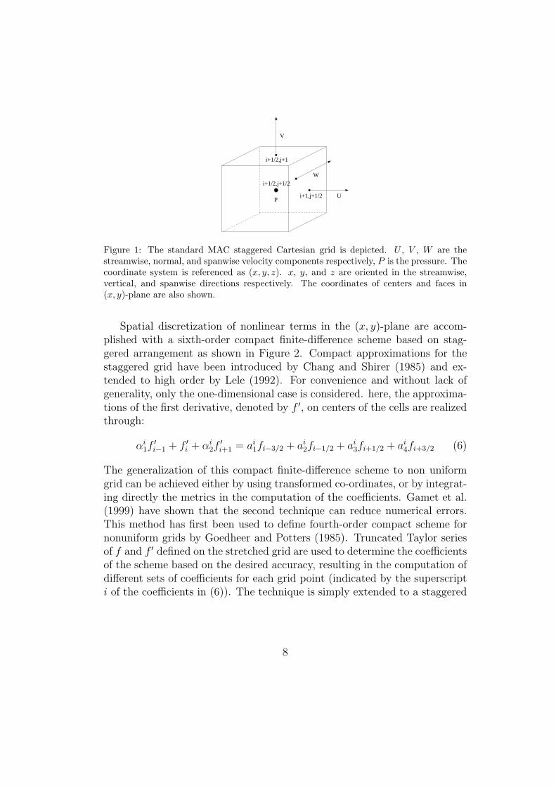
Figure 1: The standard MAC staggered Cartesian grid is depicted. U , V , W are thestreamwise, normal, and spanwise velocity components respectively, P is the pressure. Thecoordinate system is referenced as (x, y, z). x, y, and z are oriented in the streamwise,vertical, and spanwise directions respectively. The coordinates of centers and faces in(x, y)-plane are also shown.

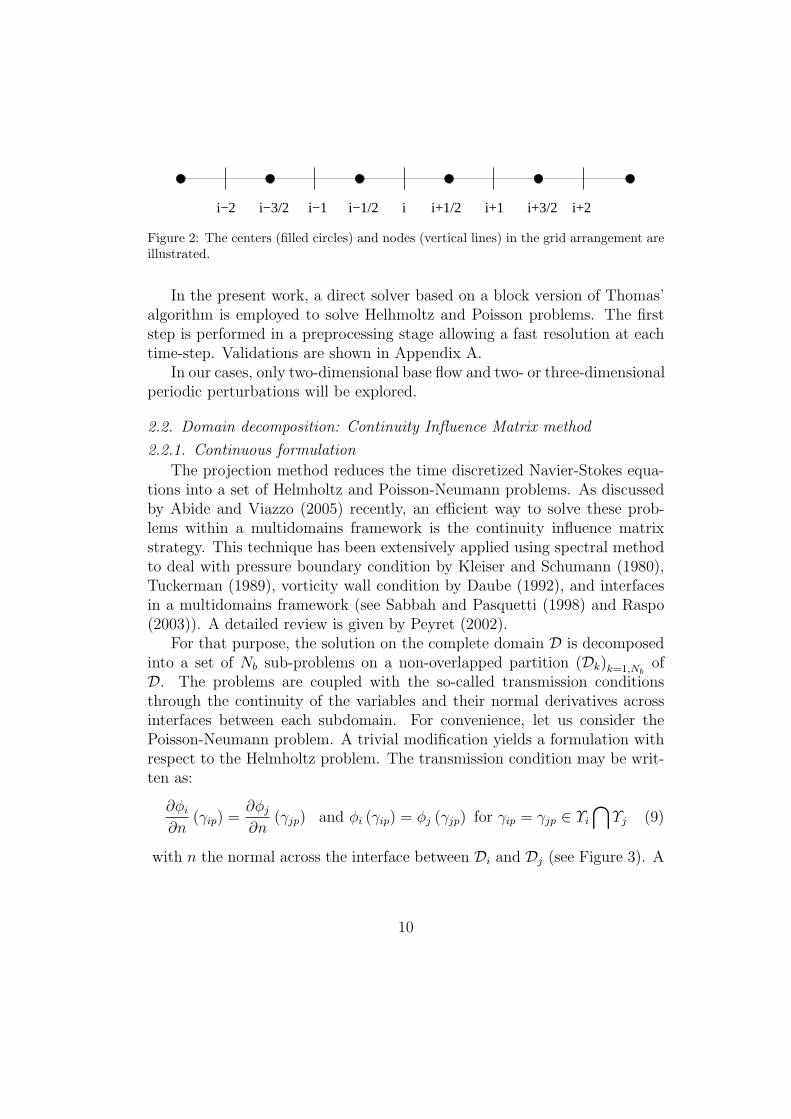
Spatial discretization of nonlinear terms in the (x, y)-plane are accom-plished with a sixth-order compact finite-difference scheme based on stag-gered arrangement as shown in Figure 2. Compact approximations for thestaggered grid have been introduced by Chang and Shirer (1985) and ex-tended to high order by Lele (1992). For convenience and without lack ofgenerality, only the one-dimensional case is considered. here, the approxima-tions of the first derivative, denoted by f ′, on centers of the cells are realizedthrough:

αi1f

′i−1 + f ′

i + αi2f

′i+1 = ai1fi−3/2 + ai2fi−1/2 + ai3fi+1/2 + ai4fi+3/2 (6)

The generalization of this compact finite-difference scheme to non uniformgrid can be achieved either by using transformed co-ordinates, or by integrat-ing directly the metrics in the computation of the coefficients. Gamet et al.(1999) have shown that the second technique can reduce numerical errors.This method has first been used to define fourth-order compact scheme fornonuniform grids by Goedheer and Potters (1985). Truncated Taylor seriesof f and f ′ defined on the stretched grid are used to determine the coefficientsof the scheme based on the desired accuracy, resulting in the computation ofdifferent sets of coefficients for each grid point (indicated by the superscripti of the coefficients in (6)). The technique is simply extended to a staggered

8

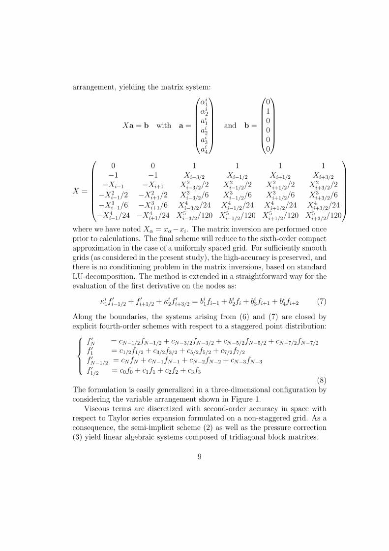
arrangement, yielding the matrix system:

Xa = b with a =

αi1

αi2

ai1ai2ai3ai4

and b =

010000

X =

0 0 1 1 1 1−1 −1 Xi−3/2 Xi−1/2 Xi+1/2 Xi+3/2

−Xi−1 −Xi+1 X2i−3/2/2 X2

i−1/2/2 X2i+1/2/2 X2

i+3/2/2

−X2i−1/2 −X2

i+1/2 X3i−3/2/6 X3

i−1/2/6 X3i+1/2/6 X3

i+3/2/6

−X3i−1/6 −X3

i+1/6 X4i−3/2/24 X4

i−1/2/24 X4i+1/2/24 X4

i+3/2/24

−X4i−1/24 −X4

i+1/24 X5i−3/2/120 X5

i−1/2/120 X5i+1/2/120 X5

i+3/2/120

where we have noted Xα = xα−xi. The matrix inversion are performed onceprior to calculations. The final scheme will reduce to the sixth-order compactapproximation in the case of a uniformly spaced grid. For sufficiently smoothgrids (as considered in the present study), the high-accuracy is preserved, andthere is no conditioning problem in the matrix inversions, based on standardLU-decomposition. The method is extended in a straightforward way for theevaluation of the first derivative on the nodes as:

κi1f′i−1/2 + f ′

i+1/2 + κi2f′i+3/2 = bi1fi−1 + bi2fi + bi3fi+1 + bi4fi+2 (7)

Along the boundaries, the systems arising from (6) and (7) are closed byexplicit fourth-order schemes with respect to a staggered point distribution:

f ′N = cN−1/2fN−1/2 + cN−3/2fN−3/2 + cN−5/2fN−5/2 + cN−7/2fN−7/2

f ′1 = c1/2f1/2 + c3/2f3/2 + c5/2f5/2 + c7/2f7/2f ′N−1/2 = cNfN + cN−1fN−1 + cN−2fN−2 + cN−3fN−3

f ′1/2 = c0f0 + c1f1 + c2f2 + c3f3

(8)The formulation is easily generalized in a three-dimensional configuration byconsidering the variable arrangement shown in Figure 1.

Viscous terms are discretized with second-order accuracy in space withrespect to Taylor series expansion formulated on a non-staggered grid. As aconsequence, the semi-implicit scheme (2) as well as the pressure correction(3) yield linear algebraic systems composed of tridiagonal block matrices.

9

i i+1/2 i+1 i+3/2 i+2i−2 i−3/2 i−1 i−1/2

Figure 2: The centers (filled circles) and nodes (vertical lines) in the grid arrangement areillustrated.

In the present work, a direct solver based on a block version of Thomas’algorithm is employed to solve Helhmoltz and Poisson problems. The firststep is performed in a preprocessing stage allowing a fast resolution at eachtime-step. Validations are shown in Appendix A.

In our cases, only two-dimensional base flow and two- or three-dimensionalperiodic perturbations will be explored.

2.2. Domain decomposition: Continuity Influence Matrix method

2.2.1. Continuous formulation

The projection method reduces the time discretized Navier-Stokes equa-tions into a set of Helmholtz and Poisson-Neumann problems. As discussedby Abide and Viazzo (2005) recently, an efficient way to solve these prob-lems within a multidomains framework is the continuity influence matrixstrategy. This technique has been extensively applied using spectral methodto deal with pressure boundary condition by Kleiser and Schumann (1980),Tuckerman (1989), vorticity wall condition by Daube (1992), and interfacesin a multidomains framework (see Sabbah and Pasquetti (1998) and Raspo(2003)). A detailed review is given by Peyret (2002).

For that purpose, the solution on the complete domain D is decomposedinto a set of Nb sub-problems on a non-overlapped partition (Dk)k=1,Nb

ofD. The problems are coupled with the so-called transmission conditionsthrough the continuity of the variables and their normal derivatives acrossinterfaces between each subdomain. For convenience, let us consider thePoisson-Neumann problem. A trivial modification yields a formulation withrespect to the Helmholtz problem. The transmission condition may be writ-ten as:

∂φi

∂n(γip) =

∂φj

∂n(γjp) and φi (γip) = φj (γjp) for γip = γjp ∈ Υi

⋂Υj (9)

with n the normal across the interface between Di and Dj (see Figure 3). A

10

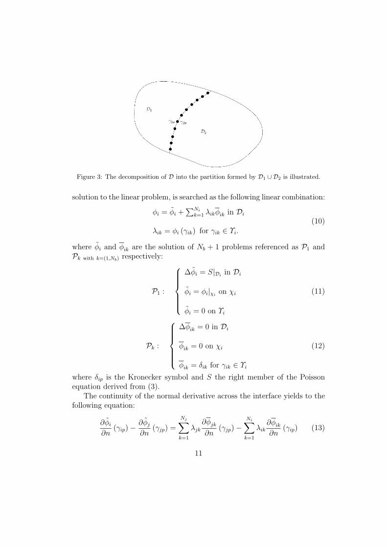
Figure 3: The decomposition of D into the partition formed by D1 ∪ D2 is illustrated.

solution to the linear problem, is searched as the following linear combination:

φi = φi +∑Ni

k=1 λikφik in Di

λik = φi (γik) for γik ∈ Υi.(10)

where φi and φik are the solution of Nb + 1 problems referenced as P1 andPk with k=(1,Nb) respectively:

P1 :

∆φi = S|Di

in Di

φi = φi|χion χi

φi = 0 on Υi

(11)

Pk :

∆φik = 0 in Di

φik = 0 on χi

φik = δik for γik ∈ Υi

(12)

where δip is the Kronecker symbol and S the right member of the Poissonequation derived from (3).

The continuity of the normal derivative across the interface yields to thefollowing equation:

∂φi

∂n(γip)−

∂φj

∂n(γjp) =

Nj∑k=1

λjk∂φjk

∂n(γjp)−

Ni∑k=1

λik∂φik

∂n(γip) (13)

11

with γip = γjp ∈ Υi⋂Υj interface values between domains i and j. Equation

(13) applied to each interface may be recast in a linear system:

MΣ = H with Σ =

λ11...λ1N1

...λjNi

...λNΥNNΥ

and H the left member provided by 13

(14)where M is the so-called continuity influence matrix. The resolution of (14)provides thus discrete values of the NΥ interfaces. The next part is devotedto emphasize how this theoretical framework is employed with a staggeredfinite difference scheme.

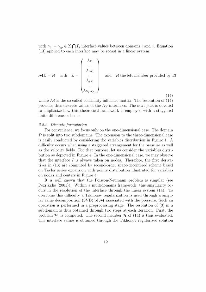
2.2.2. Discrete formulation

For convenience, we focus only on the one-dimensional case. The domainD is split into two subdomains. The extension to the three-dimensional caseis easily conducted by considering the variables distribution in Figure 1. Adifficulty occurs when using a staggered arrangement for the pressure as wellas the velocity fields. For that purpose, let us consider the variables distri-bution as depicted in Figure 4. In the one-dimensional case, we may observethat the interface I is always taken on nodes. Therefore, the first deriva-tives in (13) are computed by second-order space-decentered scheme basedon Taylor series expansion with points distribution illustrated for variableson nodes and centers in Figure 4.

It is well known that the Poisson-Neumann problem is singular (seePozrikidis (2001)). Within a multidomains framework, this singularity oc-curs in the resolution of the interface through the linear system (14). Toovercome this difficulty a Tikhonov regularization is used through a singu-lar value decomposition (SVD) of M associated with the pressure. Such anoperation is performed in a preprocessing stage. The resolution of (3) in asubdomain is thus obtained through two steps at each iteration. First, theproblem P1 is computed. The second member H of (14) is thus evaluated.The interface values is obtained through the Tikhonov regularized solution

12

1/2 1 3/2 2N−1/2N−1N−3/2N−2 I

a)

1/2 1 3/2 2N−1/2N−1N−3/2N−2 I

b)

Figure 4: The centers and nodes grid distribution used for the evaluation of the firstderivatives at the interface are depicted. The interface is denoted by I. The points takeninto account for the evaluation of the first derivative are represented in red: a) interfaceassociated with fields defined on centers: points considered are displayed in empty circles;b) interface associated with fields defined on nodes: points considered are displayed indashed lines.

of Σ. Then, the problem (15) is solved.∆φi = S|Ωi

in Ωi

φi = φi|χion χi

φi = λ on Υi

(15)

with λ the interface values of φi on Υi. Interfaces regarding Helmholtz prob-lems are obtained by means of a LU decomposition of M with respect tovelocity fields. As before, the operation is carried out in a preprocessingstage. Finally, a connectivity table is designed to ensure communicationbetween each subdomain.

3. Global linear stability: theory and numerical method

3.1. Generalities

Within a global linear stability framework, the main hypothesis is thatthe occurrence of large scale unsteadiness can be described by a bifurcation

13

theory based on the linearization of the Navier-Stokes operator about anequilibrium state. A recent review of such a method is given by Sipp et al.(2010). Here, we recall the equations governing the space-time nonlineardynamics of the flow as follows:

∂u

∂t= F (u) (16)

where u =t (u, v, w) is projected into a free-divergence space and F theNavier-Stokes operator. A two-dimensional equilibrium state of (16) is ref-erenced hereafter as U (x, y) with F (U (x, y)) = 0. The stability of such asolution is governed by the dynamical system (17).

∂u

∂t(x, t) = A (u (x, t))

u (x, y, z, t = 0) = u0

(17)

where x = (x, y, z), u is a small perturbation superimposed on U and A theJacobian operator of F about U (x, y): A = ∂F/∂U. Solutions of (17) maybe thought in the following form:

u (x, t) = e−iΩtu (x) (18)

The asymptotic stability of the system (17) is thus determined by resolv-ing the spectrum of the operator A. In particular, if Ωi > 0, the solutionF (U (x, y)) = 0 is asymptotically unstable, whose unsteadiness is character-ized by the frequency Ωr/2π and its spatial structure by u (x).

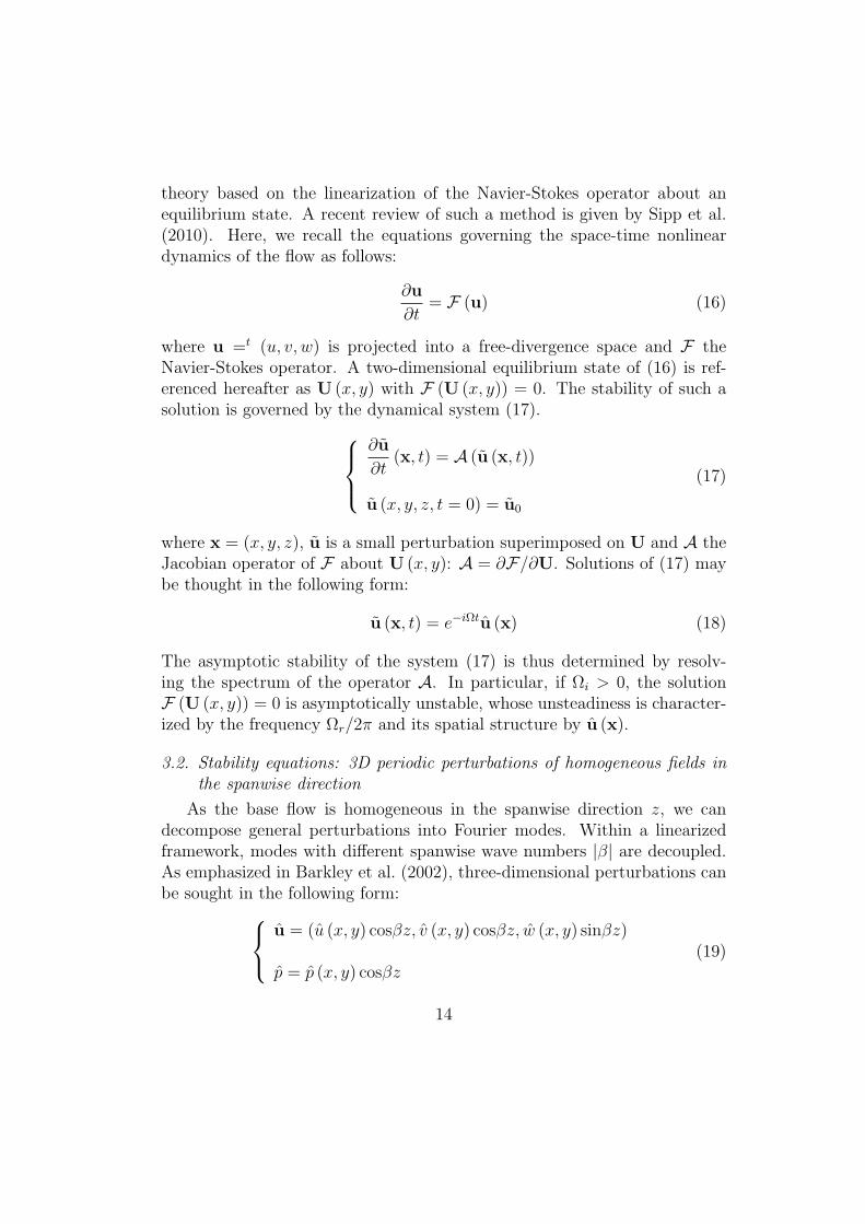
3.2. Stability equations: 3D periodic perturbations of homogeneous fields inthe spanwise direction

As the base flow is homogeneous in the spanwise direction z, we candecompose general perturbations into Fourier modes. Within a linearizedframework, modes with different spanwise wave numbers |β| are decoupled.As emphasized in Barkley et al. (2002), three-dimensional perturbations canbe sought in the following form:

u = (u (x, y) cosβz, v (x, y) cosβz, w (x, y) sinβz)

p = p (x, y) cosβz(19)

14

In order to use a linearized version of the DNS code described in previoussection, the system (17) may be rewritten in a flux conservative formulationas:

∂u

∂t+ 2

∂Uu

∂x+∂Uv

∂y+∂V u

∂y+ Uβw +

∂p

∂x=

1

Re∇2u

∂v

∂t+ 2

∂V v

∂y+∂Uv

∂x+∂V u

∂x+ V βw +

∂p

∂y=

1

Re∇2v

∂u

∂t+∂Uw

∂x+∂V w

∂y− βp =

1

Re∇2w

∂u

∂x+∂v

∂y+ βw = 0

(20)

This formulation is then well adapted to the Mac staggered grid depicted inFigure 1. The two-dimensional case is straightforward by considering β = 0.

3.3. Equilibrium state

A large variety of methods are exposed by several authors to determinethe equilibrium state F (U (x, y)) = 0 of (16). Among these, one may arguethat imposing the symmetry of the system (16) is the most obvious solu-tion. Starting from an initial guess, a Newton procedure may also be used toachieve this (see Tuckerman and Barkley (2000) and Knoll and Keyes (2004)for a recent review). Otherwise, both approaches can not be apparent orinvolve several computational efforts. An easy way to deal with the station-nary state is to consider a temporal filtering technique. This method wasfirstly employed in a global modes framework by Akervik et al. (2006). Theequations (16) are recast as:

∂U

∂t= F (U)− χ (U−Uf )

∂Uf

∂t=

U−Uf

∆

(21)

where Uf denotes the filtered velocitiy field. The filter cut-off frequency istaken as fc = f/2 with f the frequency of the unsteadiness. A differentialform of such a causal-low pass temporal filter combined with a control tech-nique allows to converge until a steady state solution which verifies F (U) = 0

15

(21). ∆ and χ are the filter width and the amplitude of the control respec-tively. By following Akervik et al. (2006), χ has to verify: Ωi < χ < Ωi+1/∆where Ωi is associated with the least damped eigenvalue. In the next part,both the symmetry method and the filtering technique are applied. Regard-ing the last method, the system (21) is solved by marching forward in timeboth the term χ (U−Uf ) and the filtering field with an AB3. A residualcriterion is based on rbf = maxD |U−Uf | as in Akervik et al. (2006).

3.4. Matrix-free framework: a multidomains strategy

Within a matrix-free framework, the dominant eigenmodes of A are ap-proximated by generating a Krylov subspace of dimension N based on severalsnapshots of the system (17) which is initiated by a perturbation u0. Sucha method is well detailed by Saad (2003) and is applied with success in sev-eral single domain configurations in both three- (Tezuka and Kojiro (2006),Bagheri et al. (2009b) and Feldman and Gelfat (2010)) and two-dimensionalgeometries (Barkley and Blackburn (2008), Bagheri et al. (2009a) and Bresand Colonius (2008)). We will briefly introduce the notations and numericalmethods within a single domain framework. The action of the operator (17)upon an initial perturbation during an evolution time interval ∆T is

u (t = ∆T ) = B (∆T ) u0, where B (∆T ) is formally eA∆T (22)

One may precise that such an operation is achieved through the system (20).A sequence of N snapshots of (17) may thus be expressed as:

SN =(u0,B (∆T ) u0,B (∆T )2 u0, ...,B (∆T )N−1 u0

)= (S1, ..., SN) (23)

An Arnoldi algorithm based on a Gram-Schmidt orthonormalization of thesequence (23), denoted by ⊥SN =

( ⊥S1, ...,⊥ SN

), leads to the following

system:B (∆T ) ⊥SN = ⊥SNH + rte⊥SN+1 (24)

with r a residual, te = (0, 0, 0, ..., 0, 1) a canonical vector of dimension N . His an upper Hessenberg matrix of dimension N × N . Therefore, the domi-nant eigenmodes of B (∆T ) are approximated through the eigenmodes of thereduced matrix H. Let us now adapt such an algorithm to our multidomainsstrategy. At first, we may point out that global unsteadiness is felt all overthe flow fields. Hence, this feature allows in processing with subdomains,by forming sequences which contain only data from each block of the full

16

domain. This idea is recently suggested by Schmid (2010). Nevertheless, theauthor has not applied this strategy in a multidomains framework. For thatpurpose, it is convenient to use the connectivity table realized in the DNScode which links all subdomains to eachothers. Subdomains are denoted by•p. The algorithm is detailed in Algorithms a). The inner product <,> isbased on the kinetic energy. An in-house code is employed to achieve suchan algorithm. Next, the matrix-free method underlying subsets of the fulldomain will be validated by Algorithms b).

17

'

&

$

%

Nb: number of subdomainsN : number of snapshotsk: eigenmode

for (p = 1, Nb)SpN = (Sp

1 , .., SpN ):

sequence of snaphsots in Di.endfor

for (p = 1, Nb)

call arnoldi(SpN , N, Ωi

pk, Ωr

pk, up

k)

endfor

Calculate uk in D1 ∪ D2... ∪ DNbby

means of the connectivity table

a) Each sudomain Di is consid-ered.'

&

$

%

Nb: number of subdomainsN : number of snapshotsk: eigenmode

for (p = 1, Nb)SpN = (Sp

1 , .., SpN ):

sequence of snaphsots in Di.endfor

SN = S1N ∪ S2

N ... ∪ SNb

N

call arnoldi(SN , N, Ωik, Ωrk, uk)

b) The full domain D is consid-ered.

'

&

$

%

while (test=0)

Orthonormalize SN : ⊥SN , by a modi-fied Gram-Schmidt algorithm

if ((maxi,j <

⊥ Si,⊥ Sj >

)< 10−16 )

for i 6= j with (i, j) ∈ (1, .., N)2

test=1

endif

endwhile

for (i = 1, N)

B (∆T ) ⊥Si = B (∆T ) (Si) −i−1∑k=1

< ⊥Sk, Si >

< ⊥Sk, ⊥Sk >Bp (∆T )

( ⊥Sk

)with B (∆T ) (Si) = (Si+1)

endfor

• Calculate H,

Hi,j =< B (∆T )⊥Si,

⊥ Sj >

• Calculate eigenvalues dk andeigenvectors uk of H with theQR routine ZGEEV from LA-PACK library

• Calculate eigenvalues ofB (∆T ):(Ωi)k = < (ln (dk) /∆T )

(Ωr)k = = (ln (dk) /∆T )

• Eigenvectors of B (∆T ): uk

c) arnoldi(SN , N, Ωik, Ωrk, uk)

Algorithms: Time-stepping strategy based on the full domain D and sub-sets of D.

4. Lid-driven cavity flow at Re = 900

In the present part, the ability as well as the accuracy of the global stabil-ity matrix-free method are assessed by computing dominant eigenmodes. Thebenchmark lid-driven cavity at Re = 900 subjected to three-dimensional per-

18

U

D1 D2

U

D2 D3

D1 D4

a)

x

100 200 3000

0.2

0.4

0.6

0.8

1

Mesh 6

Mesh 1

i

b)

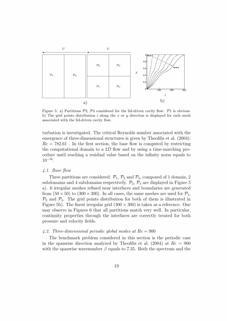
Figure 5: a) Partitions P2, P4 considered for the lid-driven cavity flow. P1 is obvious.b) The grid points distribution i along the x or y direction is displayed for each meshassociated with the lid-driven cavity flow.

turbation is investigated. The critical Reynolds number associated with theemergence of three-dimensional structures is given by Theofilis et al. (2004):Re = 782.61 . In the first section, the base flow is computed by restrictingthe computational domain to a 2D flow and by using a time-marching pro-cedure until reaching a residual value based on the infinity norm equals to10−16.

4.1. Base flow

Three partitions are considered: P1, P2 and P4, composed of 1 domain, 2subdomains and 4 subdomains respectively. P2, P4 are displayed in Figure 5a). 6 irregular meshes refined near interfaces and boundaries are generatedfrom (50× 50) to (300× 300). In all cases, the same meshes are used for P1,P2 and P4. The grid points distribution for both of them is illustrated inFigure 5b). The finest irregular grid (300× 300) is taken as a reference. Onemay observe in Figures 6 that all partitions match very well. In particular,continuity properties through the interfaces are correctly treated for bothpressure and velocity fields.

4.2. Three-dimensional periodic global modes at Re = 900

The benchmark problem considered in this section is the periodic casein the spanwise direction analyzed by Theofilis et al. (2004) at Re = 900with the spanwise wavenumber β equals to 7.35. Both the spectrum and the

19

V

U

-1 -0.8 -0.6 -0.4 -0.2 0 0.2 0.4

0

0.5

1

0 0.5 1-0.6

-0.4

-0.2

0

0.2

0.4

x

y

a)

y

x

b)

Figure 6: a) The velocity profiles in the lid-driven cavity are plotted at the mid-height andmid-length for Re = 900. The mesh (300×300) is considered. P1 is displayed in full lines.P2, and P4 are plotted with triangles and circles respectively. According to the latter,every 5 points are represented. b) The pressure fields regarding the lid-driven cavity flowat Re = 900 is shown in full lines. The partitions P1, P2 and P4 are considered .

numerical values with respect to the least damped eigenmodes obtained byTheofilis et al. (2004) are displayed in Figure 7 and in Table 1.

4.2.1. Time-stepping: validation of numerical parameters

To examine the validity of time-stepping numerical parameters, we inves-tigate the infuence of both the sampling period ∆T and the dimension of theKrylov subspace N on the modes T1, T2, T3 and S1. The algorithm detailedin Algorithms b) is employed. For demonstration purposes, we considerpartition P1 and the mesh (300× 300). ∆T is taken to verify the Nyquistcriterion (see Bagheri et al. (2009a)). In this context, we focus on the high-est frequency mode, corresponding to T2. The linear stability analysis withrespect to mode T2 is conducted by setting ∆T = TT2/32, where TT2 is theperiod associated with the mode T2, which is 16 times the Nyquist cutoff. Alarge Krylov subspace of dimension N = 600 is taken as a reference value,noted hereafter as •ref . To illustrate the accuracy of the Krylov dimensionsubspace N , an error criterion is defined by

er (Ωr) = |Ωr − (Ωr)ref

(Ωr)ref|, er (Ωi) = |

Ωi − (Ωi)ref(Ωi)ref

| (25)

20

Ωi

-4 -2 0 2 4-0.25

-0.2

-0.15

-0.1

-0.05

0

TDO2004P1

P2

P4

T2

S1

T3

T4

Ωr

Figure 7: The spectrum of the lid-driven cavity flow subjected to three-dimensional per-turbation is shown for Re = 900 and β = 7.35. Values given by Theofilis et al. (2004) arereferenced by TDO. The mesh is fixed to (300× 300). P1, P2 and P4 are considered inour computations.

Mode Ωr (TDO) Ωi (TDO) Ωr Ωi

T1 ±0.4981 −0.0043 ±0.4997 −0.0046T2 ±1.3846 −0.1044 ±1.3867 −0.1044T3 ±0.6928 −0.1071 ±0.6934 −0.1064S1 0.0000 −0.1425 0.0000 −0.1423

Table 1: The complex circular frequencies obtained by Theofilis et al. (2004) (referenced asTDO) with regards to modes T1, T2, T3 and S1. Values are compared with those computedin this manuscript by considering the full domain D (algorithm Algorithms b) and mesh(300× 300). Results are independent of partitions P1, P2 and P4 considered at numbersof significant digits given.

21

200 250 300 350 400 45010-14

10-12

10-10

10-8

10-6

10-4er(Ωr)er(Ωi)

N

a)

100 200 30010-13

10-11

10-9

10-7

10-5

10-3er(Ωr)er(Ωi)

8

3

4

N

b)

3 4 5 6 7 8

2E-11

4E-11

6E-11

Nyquist

c)

Figure 8: a), b) Mode T2 is considered. c) Mode S1 is considered. N is the Krylovdimension subspace. a) −log10

(er

(Ωr/i

))is plotted with respect to ∆T = TT2/32 where

TT2is the period of mode T2. b), c) −log10

(er

(Ωr/i

))is plotted with respect to ∆T =

TT2/8, ∆T = TT2/4 and ∆T = TT2/3.

As shown in Figure 8 a), we may observe a convergence of er with an accu-racy ≈ 10−13 until to reach a staturated value for both Ωr and Ωi. Let us nowinvestigate the influence of ∆T . For that purpose, three sampling frequenciesare chosen, corresponding to 8, 4 and 3 times the Nyquist criterion respec-tively. The values of er are depicted in Figure 8 b) by increasing the Kylovsubspace N . One may observe that up to sampling frequency of about threetimes the Nyquist cutoff, the residual error is less than 10−11. In particular,a Krylov subspace of dimension N = 100, which corresponds to approxima-tively 15 periods, is sufficient to observe a saturation of the Arnoldi algorithmregarding the largest sampling time. Therefore, this analysis suggests that asampling frequency superior to 3 times the Nyquist cutoff and a total sam-pling time larger than 15 periods are appropriate. As a consequence, theleast damped unstationnary eigenmodes T1, T2 and T3 are computed by set-ting ∆T ≈ 0.75 equals to three times the Nyquist cutoff underlying mode T2,and a Krylov subspace of dimension N = 300. Hence, both modes T1 andT3 verify the criterion defined above. Such criterion may not be defined forthe stationnary mode S1. Now, we study the influence of ∆T based on theNyquist criterion associated with T2. As above, the reference value is takenfor a frequency sampling equals to 16 times the Nyquist cutoff and N = 600.It may be observed in Figure 8 c) that the residual error is less than 10−11 byvarying the sampling frequency. It implies that the time-stepping numericalparameters defined above ensure a sufficient accuracy to calculate T1, T2, T3

22

er (Ωr)

50 100 150 200 250

10-4

10-3

10-2 T 1T 2T 3

nx/y

er (Ωi)

100 200 300

10-4

10-3

10-2

10-1

100

T 1T 2T 3

nx/y

Figure 9: Maximum relative error of the global circular frequency associated with M1, M2

and M3 as function of the mesh refinement: nx/y (number of grid points according to x/or y) for Mesh 1 → 5 (see figure 5b). Results with respect to P1, P2 and P4 are displayedin full lines, triangles and circles respectively.

and S1. For these parameters, the temporal amplification rates and circularfrequencies with regards to T1, T2, T3 and S1 are referenced in Table 1 anddisplayed in Figure 7. In addition, a good agreement is observed comparedto the data from Theofilis et al. (2004).

4.2.2. Influence of the domain decomposition

Several simulations are then carried out with different meshes as displayedin Figures 5 b). The reference values are associated with P1 and a mesh(300× 300). In order to measure the effect of the partioning on the modesT1, T2, T3, we also consider P2 and P4. The stability calculations are carriedout by considering the full domain D (algorithm Algorithms b)). er

(Ωr/i

)are plotted in Figure 9 for each partition and T1, T2 and T3. One may observethat the convergence rate is not affected by the partioning. In particular,both temporal amplificate rate and circular frequency converge to the samevalue Ωr/i (ref) associated with P1. The eigenvalues are also reported inFigure 7.

In the end, perturbation velocity fields with respect to T1 are plotted inFigure 10 regarding the finest grid mesh. Once again, it shows that continuityproperties through interfaces are well solved.

23

y

x

y

x

y

x

Figure 10: Perturbation velocity fields associated with T1 is shown. The mesh is fixed to(300× 300). P1, P2 and P4 are considered in full, dashed and dotted lines respectively.The streamwise, normal and spanwise components are ordered from the left to the right.

y

0 0.5 10

0.5

1

x

y

0 0.5 10

0.5

1

x

y

0 0.5 10

0.5

1

x

Figure 11: Partitions referenced as P4, P16 and P64 are illustrated. Every six meshes areplotted in each direction.

4.2.3. Efficiency of the algorithm

Let us now investigate the possibility of parallel computations with re-spect to our multidomains matrix-free method. For that purpose, 3 partitionsare considered denoted as P4, P16 and P64 composed by 4, 16 and 64 sub-domains respectively. The mesh grid is set to (300× 300) and are shown inFigure 11. The number of grid points in both directions x and y is equalin each subdomain. The snapshots are performed in each subdomain withrespect to P4, P16 and P64. The Arnoldi algorithm Algorithms a) is thenapplied to recover eigenmodes in the entire geometry. The mode T2 is takeninto account to illustrate our purpose. Error values defined in (25) for eachsubdomain are then computed. The reference value is defined in the previoussection. In Figure 12, we plot in a logarithmic scale, the different values ofer (Ωr) and er (Ωi). The error is about 10−4 according to Ωi and 10−5 with

24

20 40 602

3

4

5

6

7

Di

a)

20 40 605

6

7

8

Di

b)

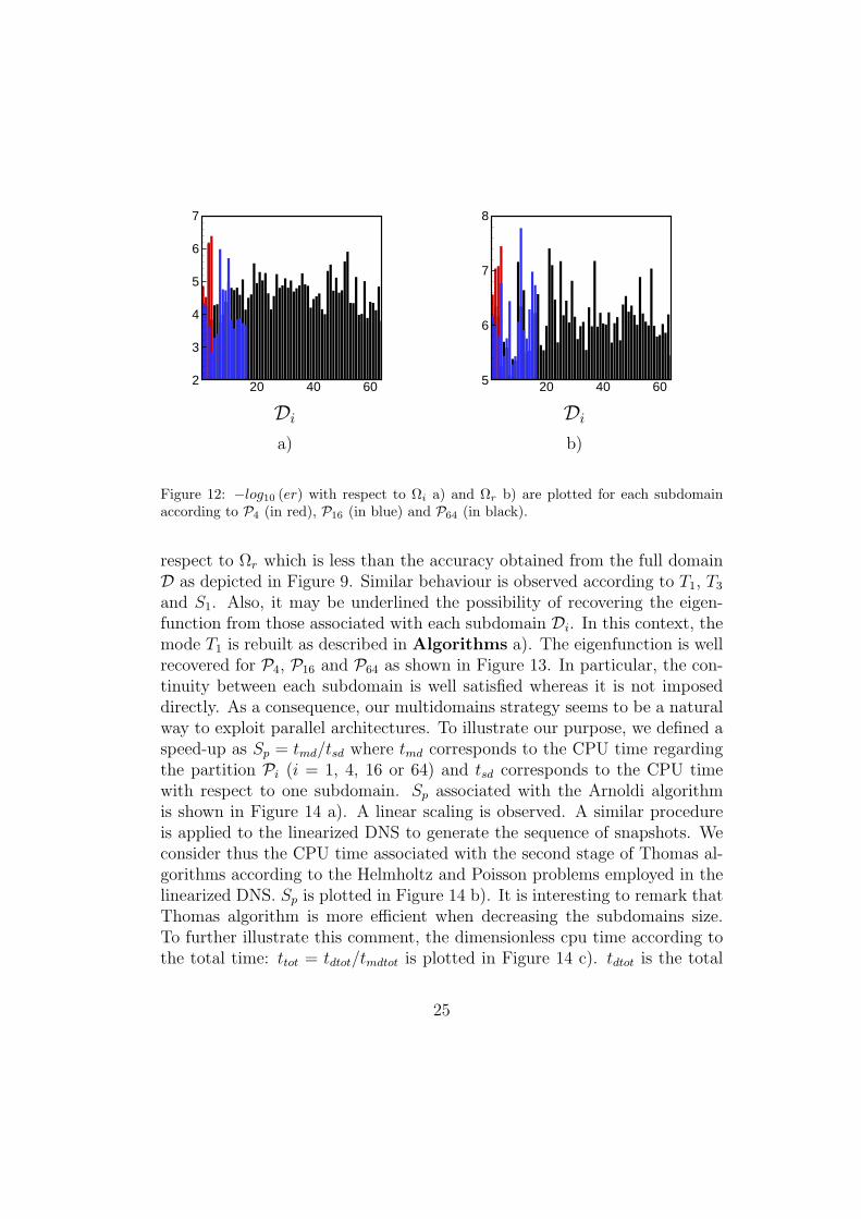
Figure 12: −log10 (er) with respect to Ωi a) and Ωr b) are plotted for each subdomainaccording to P4 (in red), P16 (in blue) and P64 (in black).

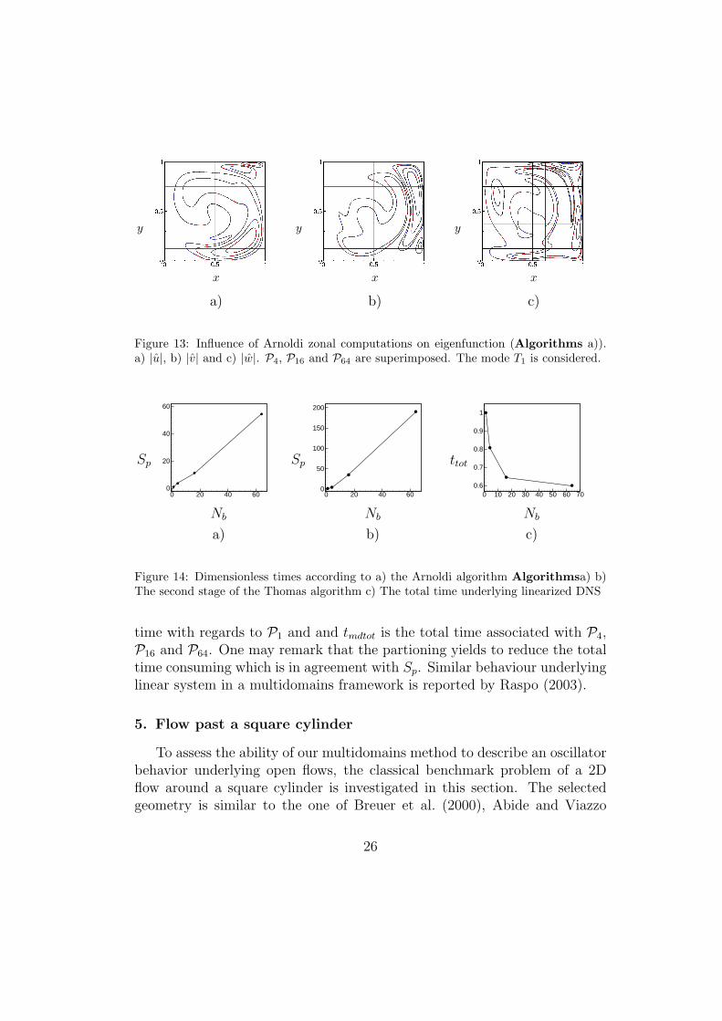
respect to Ωr which is less than the accuracy obtained from the full domainD as depicted in Figure 9. Similar behaviour is observed according to T1, T3and S1. Also, it may be underlined the possibility of recovering the eigen-function from those associated with each subdomain Di. In this context, themode T1 is rebuilt as described in Algorithms a). The eigenfunction is wellrecovered for P4, P16 and P64 as shown in Figure 13. In particular, the con-tinuity between each subdomain is well satisfied whereas it is not imposeddirectly. As a consequence, our multidomains strategy seems to be a naturalway to exploit parallel architectures. To illustrate our purpose, we defined aspeed-up as Sp = tmd/tsd where tmd corresponds to the CPU time regardingthe partition Pi (i = 1, 4, 16 or 64) and tsd corresponds to the CPU timewith respect to one subdomain. Sp associated with the Arnoldi algorithmis shown in Figure 14 a). A linear scaling is observed. A similar procedureis applied to the linearized DNS to generate the sequence of snapshots. Weconsider thus the CPU time associated with the second stage of Thomas al-gorithms according to the Helmholtz and Poisson problems employed in thelinearized DNS. Sp is plotted in Figure 14 b). It is interesting to remark thatThomas algorithm is more efficient when decreasing the subdomains size.To further illustrate this comment, the dimensionless cpu time according tothe total time: ttot = tdtot/tmdtot is plotted in Figure 14 c). tdtot is the total

25

y

x

a)

y

x

b)

y

x

c)

Figure 13: Influence of Arnoldi zonal computations on eigenfunction (Algorithms a)).a) |u|, b) |v| and c) |w|. P4, P16 and P64 are superimposed. The mode T1 is considered.

Sp

0 20 40 600

20

40

60

Nb

a)

Sp

0 20 40 600

50

100

150

200

Nb

b)

ttot

0 10 20 30 40 50 60 700.6

0.7

0.8

0.9

1

Nb

c)

Figure 14: Dimensionless times according to a) the Arnoldi algorithm Algorithmsa) b)The second stage of the Thomas algorithm c) The total time underlying linearized DNS

time with regards to P1 and and tmdtot is the total time associated with P4,P16 and P64. One may remark that the partioning yields to reduce the totaltime consuming which is in agreement with Sp. Similar behaviour underlyinglinear system in a multidomains framework is reported by Raspo (2003).

5. Flow past a square cylinder

To assess the ability of our multidomains method to describe an oscillatorbehavior underlying open flows, the classical benchmark problem of a 2Dflow around a square cylinder is investigated in this section. The selectedgeometry is similar to the one of Breuer et al. (2000), Abide and Viazzo

26

XY

0 5 10 15 20 25 3-4

-2

0

2

4

D2

D1

D3 D4

D5

D7

D6

D8

L2L1

H

D

Figure 15: Domain partitioning of the flow past a square cylinder.

(2005) and Camarri and Iollo (2010). It is composed of a square cylinderwith a diameter D = 1, centered inside a plane channel of height H = 8. Thegeometry as well as the partioning are illustrated in Figure 15. A parabolicinlet velocity profile is prescribed at the inflow. The system (1) is closedby wall and outflow boundary conditions. The Reynolds number based onmaximum inlet velocity umax and square cylinder diameter D is fixed atRe = 60, which is slightly above the critical value ≈ 58 (see Camarri andIollo (2010)).

5.1. Base flow

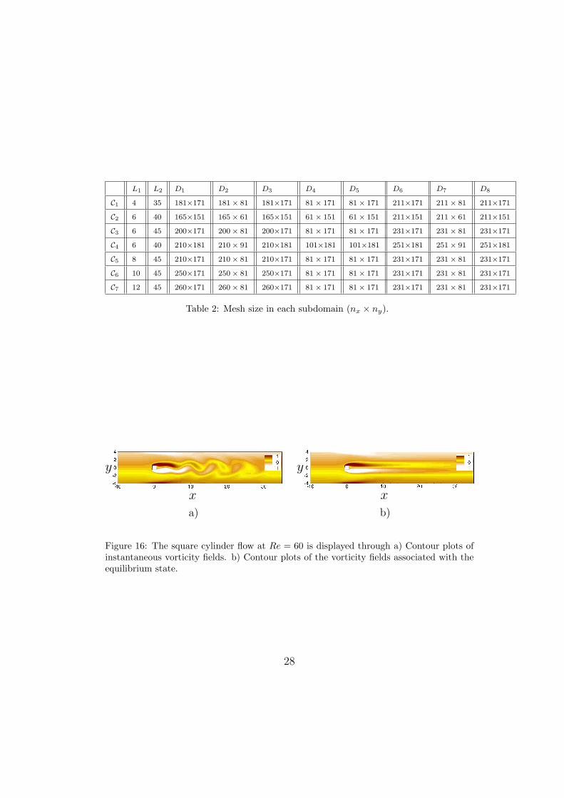
A critical point concerning open-flows is associated with the placement ofdomain boundaries. To guarantee a relevant base flow and linear dynamics,stationnary computations are carried out on 7 different meshes summed upin Table 2 referenced as Ci. Each mesh is refined near the walls of the squarecylinder and on upper as well as lower wall boundaries. The case C3 is il-lustrated in Figure 16. A Fourier analysis of the unsteady computation (seeFigure 16 a)) indicates a Strouhal number St ≈ 0.12, which is equivalent tothe value obtain by Breuer et al. (2000). The cutoff frequency and the ampli-tude of the filter are fixed to fc = St/2 and χ = 0.2 respectively. Concerningthe latter, χ is determined a posteriori by computing the temporal amplifi-cation rate with respect to the dominant eigenmode. The convergence of theequilibrium state for C3 and C4 are depicted in Figure 17 a) versus time. Onemay observe that the latter is unaffected by the grid resolution. A residualvalue ≈ 10−12 is reached after 70 periods of the vortex shedding cycle. Thebase flow is illustrated in Figure 16 b). The filtering technique has for conse-quence to symmetrize the flow which is consistent with the axial symmetry.Let us investigate the influence of geometry parameters on the convergencetoward a steady state. In Figure 17 b), the size of the recirculation lengthLr versus L1 is plotted. It appears that L1/D = 10 is sufficient to reacha converged steady state. One may precise that both influence of the grid

27

L1 L2 D1 D2 D3 D4 D5 D6 D7 D8

C1 4 35 181×171 181× 81 181×171 81× 171 81× 171 211×171 211× 81 211×171

C2 6 40 165×151 165× 61 165×151 61× 151 61× 151 211×151 211× 61 211×151

C3 6 45 200×171 200× 81 200×171 81× 171 81× 171 231×171 231× 81 231×171

C4 6 40 210×181 210× 91 210×181 101×181 101×181 251×181 251× 91 251×181

C5 8 45 210×171 210× 81 210×171 81× 171 81× 171 231×171 231× 81 231×171

C6 10 45 250×171 250× 81 250×171 81× 171 81× 171 231×171 231× 81 231×171

C7 12 45 260×171 260× 81 260×171 81× 171 81× 171 231×171 231× 81 231×171

Table 2: Mesh size in each subdomain (nx × ny).

y

xa)

y

xb)

Figure 16: The square cylinder flow at Re = 60 is displayed through a) Contour plots ofinstantaneous vorticity fields. b) Contour plots of the vorticity fields associated with theequilibrium state.

28

rbf

0 200 400 600-12

-10

-8

-6

-4

-2

0 C3

C4

V

U

T

a)

Lr/D

4 6 8 10 123.2

3.3

3.4

3.5

3.6

L1/D

b)

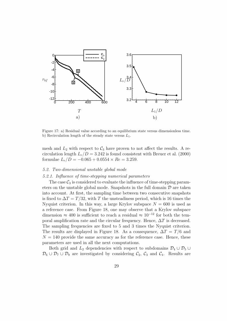
Figure 17: a) Residual value according to an equilibrium state versus dimensionless time.b) Recirculation length of the steady state versus L1.

mesh and L2 with respect to C3 have proven to not affect the results. A re-circulation length Lr/D = 3.242 is found consistent with Breuer et al. (2000)formulae Lr/D = −0.065 + 0.0554×Re = 3.259.

5.2. Two-dimensional unstable global mode

5.2.1. Influence of time-stepping numerical parameters

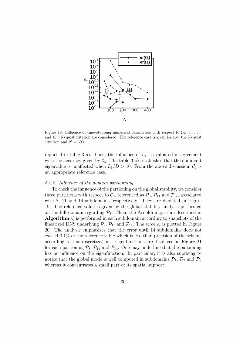
The case C3 is considered to evaluate the influence of time-stepping param-eters on the unstable global mode. Snapshots in the full domain D are takeninto account. At first, the sampling time between two consecutive snapshotsis fixed to ∆T = T/32, with T the unsteadiness period, which is 16 times theNyquist criterion. In this way, a large Krylov subspace N = 600 is used asa reference case. From Figure 18, one may observe that a Krylov subspacedimension ≈ 400 is sufficient to reach a residual ≈ 10−12 for both the tem-poral amplification rate and the circular frequency. Hence, ∆T is decreased.The sampling frequencies are fixed to 5 and 3 times the Nyquist criterion.The results are displayed in Figure 18. As a consequence, ∆T = T/6 andN = 140 provide the same accuracy as for the reference case. Hence, theseparameters are used in all the next computations.

Both grid and L2 dependencies with respect to subdomains D4 ∪ D5 ∪D6 ∪ D7 ∪ D8 are investigated by considering C2, C3 and C4. Results are

29

er

100 200 300 40010-1510-1410-1310-1210-1110-1010-910-810-710-6

er(Ωr)er(Ωi)

316

5

N

Figure 18: Influence of time-stepping numerical parameters with respect to C3. 3×, 5×and 16× Nyquist criterion are considered. The reference case is given for 16× the Nyquistcriterion and N = 600.

reported in table 3 a). Then, the influence of L1 is evaluated in agreementwith the accuracy given by C3. The table 3 b) establishes that the dominanteigenvalue is unaffected when L1/D > 10. From the above discussion, C6 isan appropriate reference case.

5.2.2. Influence of the domain partionning

To check the influence of the partioning on the global stability, we considerthree partitions with respect to C6, referenced as P8, P11 and P14, associatedwith 8, 11 and 14 subdomains, respectively. They are depicted in Figure19. The reference value is given by the global stability analysis performedon the full domain regarding P8. Then, the Arnoldi algorithm described inAlgorithm a) is performed in each subdomain according to snapshots of thelinearized DNS underlying P8, P11 and P14. The error er is plotted in Figure20. The analysis emphasizes that the error until 14 subdomains does notexceed 0.1% of the reference value which is less than precision of the schemeaccording to this discretization. Eigenfunctions are displayed in Figure 21for each partioning P8, P11 and P14. One may underline that the partioninghas no influence on the eigenfunction. In particular, it is also suprising tonotice that the global mode is well computed in subdomains D1, D2 and D3

whereas it concentrates a small part of its spatial support.

30

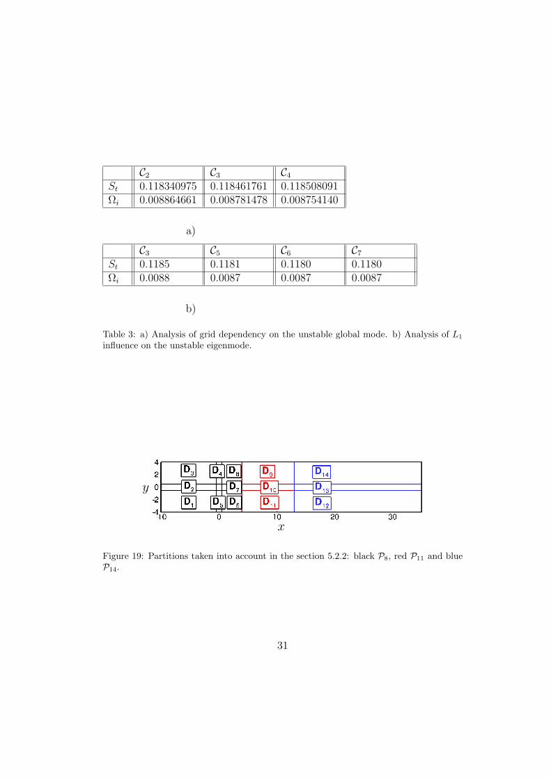
C2 C3 C4St 0.118340975 0.118461761 0.118508091Ωi 0.008864661 0.008781478 0.008754140

a)

C3 C5 C6 C7St 0.1185 0.1181 0.1180 0.1180Ωi 0.0088 0.0087 0.0087 0.0087

b)

Table 3: a) Analysis of grid dependency on the unstable global mode. b) Analysis of L1

influence on the unstable eigenmode.

y

x

Figure 19: Partitions taken into account in the section 5.2.2: black P8, red P11 and blueP14.

31

−log10 (er)

0 5 10 150

5

10

15

Di

a) Ωr

−log10 (er)

0 5 10 150

5

10

15

Di

b) Ωi

Figure 20: Error er analysis in each subdomains with respect to partioning P8, P11 andP14 (see Figure 19).

y

xa) The streamwise component u

y

xb) The normal component v

Figure 21: Perturbation velocity fields associated with the square cylinder at Re = 60.The linear global stability analysis performed on the full domain regarding P8 is displayedin flood. The analysis on subsets according to P8, P11 and P14 are displayed in full lines.

32

6. Flow past over an open cavity

The main feature of low-Mach-number open cavity flows consists of thegeneration of vortices at the leading edge of the cavity arising from Kelvin-Helmholtz instability. Their advection along the shear layer yields impinge-ment at the trailing edge and injection of vortical structures inside the cavity.This kind of instability is referred to as shear-layer mode or Rossiter mode.Recently, some aspects of three-dimensional features have been investigatedin a compressible regime by Bres and Colonius (2008). They showed that,besides the shear-layer mode, additional three-dimensional lower frequencymodes could exist which are mainly localized inside the cavity. From theabove discussion, it appears that aside its physical interest, the descriptionof the disturbance behaviour of such a flow is a wonderful numerical bench-mark concerning the efficiency of the method to deal with a wide varietyof instability phenomena in multi-connected rectangular geometries. Thiscase is designed by the ANR CORMORED where the LIMSI laboratoryand Dynfluid are participating (see Basley et al. (2010) and Alizard et al.(2010a)).

We consider the flow over a square cavity at Reynolds number ReL = 8140based on the cavity length L and free-stream velocity U∞. The Reynoldsnumber is built as ReL = U∞L/ν, ν the kinematic viscosity of air: ν =1.5× 10−5m2s−1, L = 0.1m and U∞ ≈ 1.22ms−1.

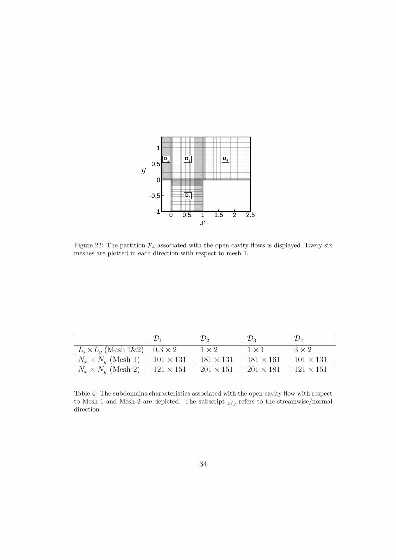
Four domains are investigated as depicted in Figure 22. On the left-handside of the leading edge of the cavity, a Blasius profile is initiated at theinflow. The distance from the leading edge is fixed to x = 4.9. On the right-hand side of the trailing edge, an outflow Neumann condition is imposed.The grid points are clustered near interfaces and walls. To dissipate vorticalstructures at the outflow, a grid stretching is implemented. Two meshes areconsidered. They are displayed in table 4.

6.1. Base flow at ReL = 8140

The two dimensional dynamics is characterized by self-sustained oscilla-tions with respect to the shear layer above the cavity driving injection ofeddies inside. Such a mechanism is illustrated in Figure 23 a). A spectralanalysis of a time series sample with regards to the vertical velocity, in themiddle of the shear layer at the top of the cavity, is performed. The Strouhalnumber is defined by St = fL/U∞, with f the characteristic frequency. Thefundamental frequency is found to be associated with St ≈ 0.89. Inspired by

33

y

0 0.5 1 1.5 2 2.5-1

-0.5

0

0.5

1

D1 D2

D3

D4

x

Figure 22: The partition P4 associated with the open cavity flows is displayed. Every sixmeshes are plotted in each direction with respect to mesh 1.

D1 D2 D3 D4

Lx×Ly (Mesh 1&2) 0.3× 2 1× 2 1× 1 3× 2Nx ×Ny (Mesh 1) 101× 131 181× 131 181× 161 101× 131Nx ×Ny (Mesh 2) 121× 151 201× 151 201× 181 121× 151

Table 4: The subdomains characteristics associated with the open cavity flow with respectto Mesh 1 and Mesh 2 are depicted. The subscript x/y refers to the streamwise/normaldirection.

34

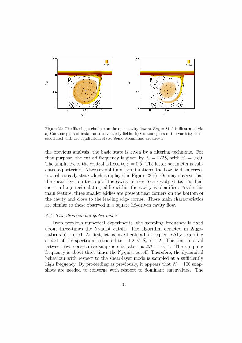
y

x

y

x

Figure 23: The filtering technique on the open cavity flow at ReL = 8140 is illustrated viaa) Contour plots of instantaneous vorticity fields. b) Contour plots of the vorticity fieldsassociated with the equilibrium state. Some streamlines are shown.

the previous analysis, the basic state is given by a filtering technique. Forthat purpose, the cut-off frequency is given by fc = 1/2St with St = 0.89.The amplitude of the control is fixed to χ = 0.5. The latter parameter is vali-dated a posteriori. After several time-step iterations, the flow field convergestoward a steady state which is diplayed in Figure 23 b). On may observe thatthe shear layer on the top of the cavity relaxes to a steady state. Further-more, a large recirculating eddie within the cavity is identified. Aside thismain feature, three smaller eddies are present near corners on the bottom ofthe cavity and close to the leading edge corner. These main characteristicsare similar to those observed in a square lid-driven cavity flow.

6.2. Two-dimensional global modes

From previous numerical experiments, the sampling frequency is fixedabout three-times the Nyquist cutoff. The algorithm depicted in Algo-rithms b) is used. At first, let us investigate a first sequence S1N regardinga part of the spectrum restricted to −1.2 < St < 1.2. The time intervalbetween two consecutive snapshots is taken as ∆T = 0.14. The samplingfrequency is about three times the Nyquist cutoff. Therefore, the dynamicalbehaviour with respect to the shear-layer mode is sampled at a sufficientlyhigh frequency. By proceeding as previously, it appears that N = 100 snap-shots are needed to converge with respect to dominant eigenvalues. The

35

a)

Ωi

-1.5 -1 -0.5 0 0.5 1 1.5-0.8

-0.6

-0.4

-0.2

0

0.2Mesh 1Mesh 2

St

b)

Ωi

-0.4 -0.2 0 0.2 0.4-0.15

-0.1

-0.05

0

Mc3

Mc1Mc2

Mc4

St

Figure 24: The spectrum according to the 2D dynamics of the flow past an open cavity atReL = 8140 is shown in a). b) A zoom of the centered part of the spectrum a) is depicted.

extracted spectrum, composed of 6 eigenvalues, is displayed in Figure 24.Only the case St > 0 is considered, since eigenvalues come in complex con-jugate pairs. Ordering modes with regards to their temporal amplificationrate, the first, second and third mode oscillate with S1

t = 0.893, S2t = 0.560

and S3t = 1.146. Only one unstable mode is identified which is unsteady

and whose the oscillatory frequency is comparable to the shear-layer modeobserved in DNS. The spatial structures of each mode are depicted in Figure25 using the streamwise and normal velocity components. The energy of theunstable mode has a most significant part inside the shear layer above thecavity. In addition, small-scale features are observed along the shear layerinside the cavity detaching from the trailing edge corner. Overall, it showsgood similarities both in terms of spatial wavelength and location with theobserved instability in DNS. Global modes with respect to S2

t and S3t con-

tain similar characteristics. The convergence property with respect to thegrid mesh is now investigated. By considering meshes displayed in Table 4,results appear to differ less than 1% in relative error (see Figure 24).

Aside from this branch, typical spectrum mainly associated with the sta-ble dynamics inside the cavity with lower frequencies are observed in simi-lar configuration by Schmid (2010) and Barbagallo et al. (2009). For thatpurpose, a second sequence S2N is considered. A part of the spectrum re-

36

a)

y

x

b)

y

x

c)

y

xd)

y

x

e)

y

x

f)

y

x

Figure 25: The spatial structures of global modes associated with those displayed in redin Figure 24 a) ordered from the left to the right according to their frequency (S2

t , S1t and

S3t respectively). The perturbation is visualized by plotting the streamwise component in

a), b), c) and the normal component in d), e), f). The unstable mode corresponds to b)and e).

37

Mc1

y

x

Mc2

y

xMc3

y

x

Mc4

y

x

Figure 26: The streamwise velocity components of modes displayed in Figure 24b) areshown.

stricted to −0.17 < St < 0.17 is explored. Hence, sampling time is fixedto ∆T = 0.1. As in the previous section, experiments on Krylov subspacedimension N show that the convergence requires the use of 200 snapshots.The corresponding spectrum is superimposed on the previous one in Figure24. A typical parabolic stable branch of lower frequencies is distinguished.The modes referenced as MC1, MC2, MC3 and MC4 in Figure 24 are illus-trated through the streamwise velocity component in Figure 26. One mayremark that a major portion is concentrated inside the cavity. These modesare characterized by a cycle of growing and decaying disturbances as it ro-tates around the main eddie. Furthermore, it shows an increase of moresmall-scales features inside the cavity with an increase in terms of frequency.Finally, one may recongnize a slight influence of the modes along the shearlayer above the cavity. Our results are consistent with the observations ofSchmid (2010) and Barbagallo et al. (2009). As a consequence, one may beconfident about our numerical method to capture this flow dynamics. Then,

38

Ωi

-1.5 -1 -0.5 0 0.5 1 1.5-0.2

-0.15

-0.1

-0.05

0

0.05

0.1

β= 0

β= 0.5

β= 1

St

Ωi

-0.1 -0.05 0 0.05 0.10

0.02

0.04

0.06

0.08

0.1

0.12

0.141

2

3

4

5

St

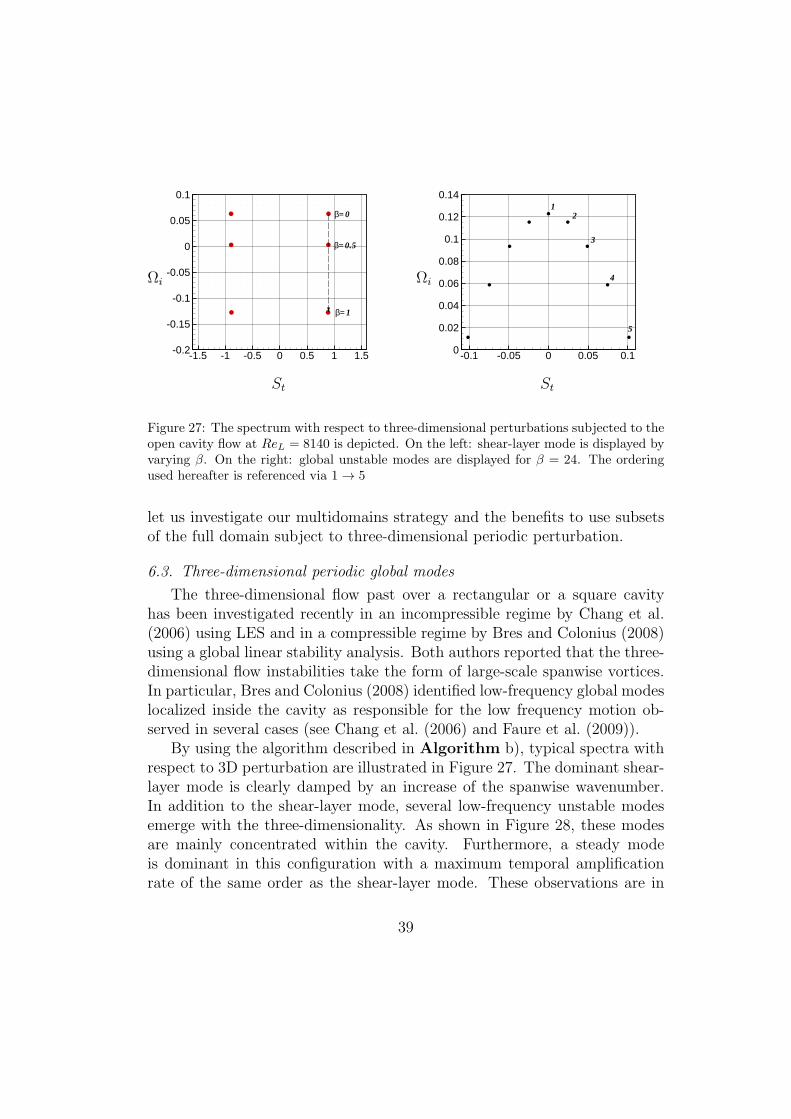
Figure 27: The spectrum with respect to three-dimensional perturbations subjected to theopen cavity flow at ReL = 8140 is depicted. On the left: shear-layer mode is displayed byvarying β. On the right: global unstable modes are displayed for β = 24. The orderingused hereafter is referenced via 1 → 5

let us investigate our multidomains strategy and the benefits to use subsetsof the full domain subject to three-dimensional periodic perturbation.

6.3. Three-dimensional periodic global modes

The three-dimensional flow past over a rectangular or a square cavityhas been investigated recently in an incompressible regime by Chang et al.(2006) using LES and in a compressible regime by Bres and Colonius (2008)using a global linear stability analysis. Both authors reported that the three-dimensional flow instabilities take the form of large-scale spanwise vortices.In particular, Bres and Colonius (2008) identified low-frequency global modeslocalized inside the cavity as responsible for the low frequency motion ob-served in several cases (see Chang et al. (2006) and Faure et al. (2009)).

By using the algorithm described in Algorithm b), typical spectra withrespect to 3D perturbation are illustrated in Figure 27. The dominant shear-layer mode is clearly damped by an increase of the spanwise wavenumber.In addition to the shear-layer mode, several low-frequency unstable modesemerge with the three-dimensionality. As shown in Figure 28, these modesare mainly concentrated within the cavity. Furthermore, a steady modeis dominant in this configuration with a maximum temporal amplificationrate of the same order as the shear-layer mode. These observations are in

39

Figure 28: The 3D global mode for β = 24 with respect to the spectrum in Figure 27 arevizualized via their spanwise component of the perturbation. The ordering is similar as inFigure 27.

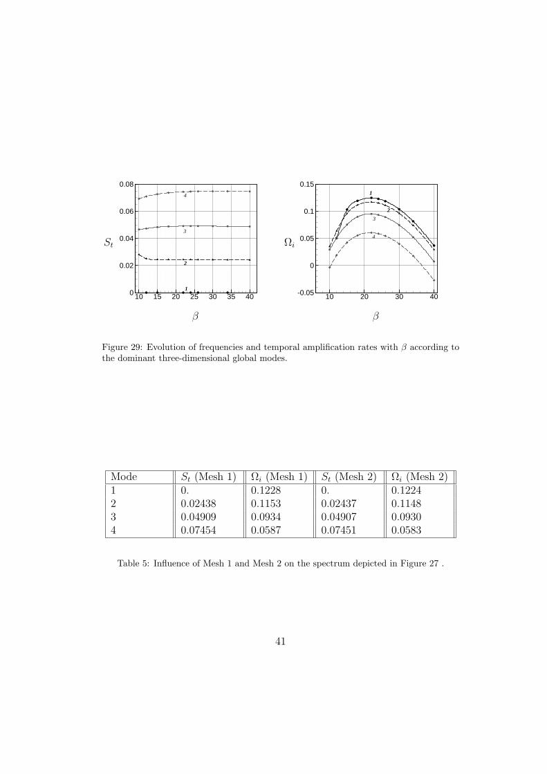
agreement with the study of Bres and Colonius (2008) in a compressibleregime. Within a large range of spanwise wave numbers, its temporalamplification rate depicted in Figure 29 rises to a maximum Ωi = 0.125for β = 22 corresponding to a wavelength λ = 2π/β ≈ 0.3. This valueis in accordance with the one obtained in a compressible regime by Bresand Colonius (2008). Indeed, the authors reported dominant wavelengthvalues equals to λ = 0.5 and λ = 0.4 associated with Mach numbers 0.6and 0.3, respectively, in a similar configuration. In the incompressible limit,our value is closed to the one estimated by Bres and Colonius (2008). Theinfluence of meshes is reported in table 5. One may observe differences on thecharacteristic variables which do not exceed 0.4%. The influence of domainssubdivision on global modes is examined.

40

St

10 15 20 25 30 35 400

0.02

0.04

0.06

0.08

2

1

4

3

β

Ωi

10 20 30 40-0.05

0

0.05

0.1

0.15

2

1

3

4

β

Figure 29: Evolution of frequencies and temporal amplification rates with β according tothe dominant three-dimensional global modes.

Mode St (Mesh 1) Ωi (Mesh 1) St (Mesh 2) Ωi (Mesh 2)1 0. 0.1228 0. 0.12242 0.02438 0.1153 0.02437 0.11483 0.04909 0.0934 0.04907 0.09304 0.07454 0.0587 0.07451 0.0583

Table 5: Influence of Mesh 1 and Mesh 2 on the spectrum depicted in Figure 27 .

41

y

0 0.5 1 1.5 2 2.5-1

-0.5

0

0.5

1

D3D7 D4 D8

D2

D1

D5

D6

x

Figure 30: The partition P8 associated with the open cavity flows is displayed. Every sixmeshes are plotted in each direction with respect to mesh 1.

6.4. Influence of domains decomposition

In the following section, the mesh 1 is considered and β = 24. Thereference values are associated with the full domain analysis based on thealgorithm depicted in Algorithms b) and P4. Two partitions of D areanalyzed, referenced as P4 and P8 corresponding to 4 and 8 subdomainsrespectively. The snaphsots are performed on each subdomain, derived froma linearized DNS for P4 and P8. The domains Di with regards to P4 andP8 are shown in Figures 22 and 30 respectively. Errors −log10 (er) in eachsubdomain for P4 and P8 are illustrated in Figure 31 with respect to modes2 and 4. Regarding P4, we observe that within the subset composed of D3

the error is minimized. It is physically relevant because spatial supportsassociated with modes 2 and 4 are mainly concentrated inside D3. However,it is also suprising to notice that the unsteadiness is also well captured in D1,D2 andD4. In particular, the error is lower than the precision of the numericalmethod as estimated in the previous section. From these encouraging results,the partition P8 is now investigated, where the subdomain D3 is divided into4 subdomains. Results are reported in Figure 31 e),f),g),h). It is interestingto note that errors with respect to Di which belong to P8, do not increasecompared to those of P4. Consequently, the partitioning does not affect thelinear dynamics. The eigenfunctions with regards to P4 and P8 computedfrom the algorithm based on subdomainsAlgorithms a) are shown in Figure32. One may remark that the full spatial support is well recovered from the

42

0 1 2 3 4 50

5

10

15

Di

a) Ωr (2)

0 1 2 3 4 50

5

10

15

Di

b) Ωi (2)

0 1 2 3 4 50

5

10

15

Di

c) Ωr (4)

0 1 2 3 4 50

5

10

15

Di

d) Ωi (4)

0 2 4 6 80

2

4

6

Di

e) Ωr (2)

0 2 4 6 80

2

4

6

Di

f) Ωi (2)

0 2 4 6 80

2

4

6

Di

g) Ωr (4)

0 2 4 6 80

2

4

6

Di

h) Ωi (4)

Figure 31: Error −log10 (er) analysis according to each subdomain with respect to parti-tions P4 and P8 and modes 2 and 4.

y

x

a) Mode 2

y

x

b) Mode 4

Figure 32: The spanwise perturbation velocity fields |wr| is plotted with respect to modes2 and 4 according to P4 (in flood) and P8 (in dashed lines).

43

partitions P4 and P8. Similar observations could be established for modes 1and 3.

7. Conclusions and prospects

This survey revisits a matrix-free method devoted to the global linearstability analysis based on a multidomains Direct Numerical Simulation code.A continuity influence matrix technique is introduced to solve grid pointslying on interfaces between subdomains. A connectivity table is used tomanage communication between each subdomain.

Through three benchmark problems, the lid-driven cavity flow and twoopen flows: the square cylinder and the open-cavity flows, it is demonstratedthat no loss of accuracy occurs when the entire computational domain ispartionned into several subdomains.

Furthermore, extracting global modes provided from snapshots basedmerely on a subset of the entire flow field appears to not induce errors supe-rior to the scheme precision. Moreover, it reproduces adequately the entireperturbation velocity fields by means of the connectivity table.

This is quite encouraging in terms of reducing the storage requirementassociated with large computational domains. This method may also be ofgreat interest to avoid contamination of global modes by boundary condi-tions, compared to a matrix method. Moreover, the multidomains strategyseems to be a natural way to exploit parallel architectures. In particular,the fact that we use the same partition with regards to the linearized DNSand the Arnoldi procedure should be usefull to couple both algorithms. Animplicitly restarded Arnoldi method relying on subspace iterations, similaras the one developed in ARPACK (Lehoucq et al. (1998)), could improve theefficiency of the global numerical method, for instance.

In addition, further developments dealing with curvilinear geometries bymeans of a coordinate transformation are also in progress.

Finally, our objective aims to simulate and extract three-dimensional flowdynamics in both linear and nonlinear regime of multi-connected rectangu-lar domains based on three-dimensional periodic base flows. Preliminarywork about the second bifurcation of a flow passing over an open cavity isin progress. Moreover, our matrix-free method combined with a Koopmanmodes solver (see Schmid (2010)) seems to be a promising tool to deal withspectral analysis according to three-dimensional nonlinear dynamics. Note

44

that a first attempt by considering the nonlinear regime of an open cav-ity flow within a two-dimensional framework has been recently adressed byAlizard et al. (2010c).

Acknowledgments

This work has received support from the National Agency for Researchon reference BLAN08−1 309235. Computing time was provided by ”Institutdu Developpement et des Ressources en Informatique Scientifique (IDRIS)-CNRS”.

8. Appendix A: irregular staggered compact finite difference schemevalidation

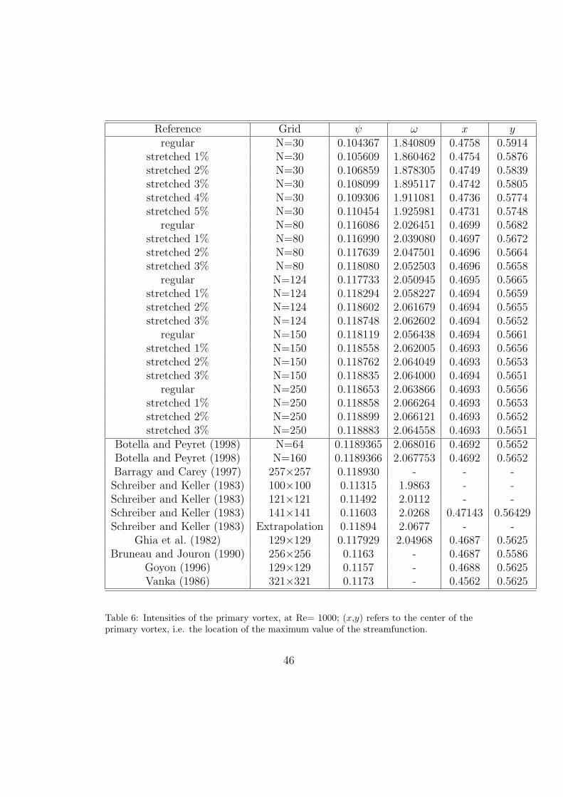
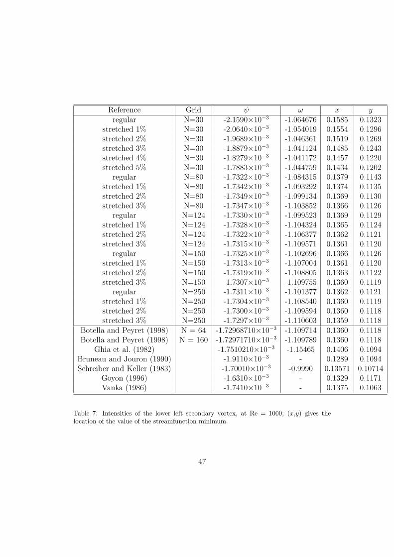
Numerical validations of the single-domain solver are reported in Chichep-ortiche et al. (2008) for a 2-D lid-driven cavity at Reynolds 1000. The sameconfiguration is used to investigate the accuracy of the formulation developedfor non uniform grids. In Tables 6 to 8, the values of the intensity of theprimary, lower left secondary, and lower right secondary vortices respectivelyare compared to selected results of the litterature. The spectral simulationsof Botella and Peyret (1998) constitute the reference. Compared to othernumerical strategies, the present results are closer to the spectral referencefor a given mesh size. The accuracy is also demonstrated by the comparisonof the extrema of the vertical velocity through the centerlines of the cavity inTable 8, and in Figure 33. The L1-norm of the error with respect to Botellaand Peyret (1998) is significantly reduced when using a Cartesian grid clus-tered near the walls with a geometric rate of 1 to 3%. The best results areobtained with a rate of 3%, and at least a second-order accuracy is obtainedwith the most defavorable choice for the mesh spacing (the minimum value),which is the leading order expected since the viscous term are discretizedwith second-order formulas (and obtained for instance for regular meshes).

45

Reference Grid ψ ω x yregular N=30 0.104367 1.840809 0.4758 0.5914

stretched 1% N=30 0.105609 1.860462 0.4754 0.5876stretched 2% N=30 0.106859 1.878305 0.4749 0.5839stretched 3% N=30 0.108099 1.895117 0.4742 0.5805stretched 4% N=30 0.109306 1.911081 0.4736 0.5774stretched 5% N=30 0.110454 1.925981 0.4731 0.5748

regular N=80 0.116086 2.026451 0.4699 0.5682stretched 1% N=80 0.116990 2.039080 0.4697 0.5672stretched 2% N=80 0.117639 2.047501 0.4696 0.5664stretched 3% N=80 0.118080 2.052503 0.4696 0.5658




Botella and Peyret (1998) N=64 0.1189365 2.068016 0.4692 0.5652Botella and Peyret (1998) N=160 0.1189366 2.067753 0.4692 0.5652Barragy and Carey (1997) 257×257 0.118930 - - -Schreiber and Keller (1983) 100×100 0.11315 1.9863 - -Schreiber and Keller (1983) 121×121 0.11492 2.0112 - -Schreiber and Keller (1983) 141×141 0.11603 2.0268 0.47143 0.56429Schreiber and Keller (1983) Extrapolation 0.11894 2.0677 - -

Ghia et al. (1982) 129×129 0.117929 2.04968 0.4687 0.5625Bruneau and Jouron (1990) 256×256 0.1163 - 0.4687 0.5586

Goyon (1996) 129×129 0.1157 - 0.4688 0.5625Vanka (1986) 321×321 0.1173 - 0.4562 0.5625

Table 6: Intensities of the primary vortex, at Re= 1000; (x,y) refers to the center of theprimary vortex, i.e. the location of the maximum value of the streamfunction.

46

Reference Grid ψ ω x yregular N=30 -2.1590×10−3 -1.064676 0.1585 0.1323

stretched 1% N=30 -2.0640×10−3 -1.054019 0.1554 0.1296stretched 2% N=30 -1.9689×10−3 -1.046361 0.1519 0.1269stretched 3% N=30 -1.8879×10−3 -1.041124 0.1485 0.1243stretched 4% N=30 -1.8279×10−3 -1.041172 0.1457 0.1220stretched 5% N=30 -1.7883×10−3 -1.044759 0.1434 0.1202

regular N=80 -1.7322×10−3 -1.084315 0.1379 0.1143stretched 1% N=80 -1.7342×10−3 -1.093292 0.1374 0.1135stretched 2% N=80 -1.7349×10−3 -1.099134 0.1369 0.1130stretched 3% N=80 -1.7347×10−3 -1.103852 0.1366 0.1126




Botella and Peyret (1998) N = 64 -1.72968710×10−3 -1.109714 0.1360 0.1118Botella and Peyret (1998) N = 160 -1.72971710×10−3 -1.109789 0.1360 0.1118

Ghia et al. (1982) -1.7510210×10−3 -1.15465 0.1406 0.1094Bruneau and Jouron (1990) -1.9110×10−3 - 0.1289 0.1094Schreiber and Keller (1983) -1.70010×10−3 -0.9990 0.13571 0.10714

Goyon (1996) -1.6310×10−3 - 0.1329 0.1171Vanka (1986) -1.7410×10−3 - 0.1375 0.1063

Table 7: Intensities of the lower left secondary vortex, at Re = 1000; (x,y) gives thelocation of the value of the streamfunction minimum.

47

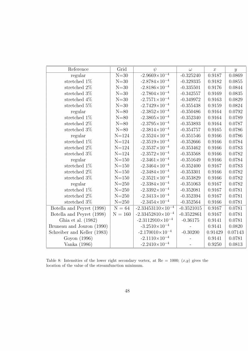
Reference Grid ψ ω x yregular N=30 -2.9669×10−4 -0.325240 0.9187 0.0869

stretched 1% N=30 -2.8784×10−4 -0.329335 0.9182 0.0855stretched 2% N=30 -2.8186×10−4 -0.335501 0.9176 0.0844stretched 3% N=30 -2.7804×10−4 -0.342557 0.9169 0.0835stretched 4% N=30 -2.7571×10−4 -0.349972 0.9163 0.0829stretched 5% N=30 -2.7429×10−4 -0.355438 0.9159 0.0824





Botella and Peyret (1998) N = 64 -2.33453110×10−4 -0.3521015 0.9167 0.0781Botella and Peyret (1998) N = 160 -2.33452810×10−4 -0.3522861 0.9167 0.0781

Ghia et al. (1982) -2.3112910×10−4 -0.36175 0.9141 0.0781Bruneau and Jouron (1990) -3.2510×10−4 - 0.9141 0.0820Schreiber and Keller (1983) -2.170010×10−4 -0.30200 0.91429 0.07143

Goyon (1996) -2.1110×10−4 - 0.9141 0.0781Vanka (1986) -2.2410×10−4 - 0.9250 0.0813

Table 8: Intensities of the lower right secondary vortex, at Re = 1000; (x,y) gives thelocation of the value of the streamfunction minimum.

48

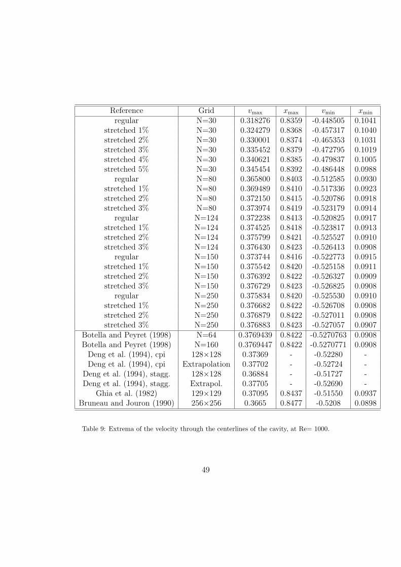
Reference Grid vmax xmax vmin xmin

regular N=30 0.318276 0.8359 -0.448505 0.1041stretched 1% N=30 0.324279 0.8368 -0.457317 0.1040stretched 2% N=30 0.330001 0.8374 -0.465353 0.1031stretched 3% N=30 0.335452 0.8379 -0.472795 0.1019stretched 4% N=30 0.340621 0.8385 -0.479837 0.1005stretched 5% N=30 0.345454 0.8392 -0.486448 0.0988

regular N=80 0.365800 0.8403 -0.512585 0.0930stretched 1% N=80 0.369489 0.8410 -0.517336 0.0923stretched 2% N=80 0.372150 0.8415 -0.520786 0.0918stretched 3% N=80 0.373974 0.8419 -0.523179 0.0914




Botella and Peyret (1998) N=64 0.3769439 0.8422 -0.5270763 0.0908Botella and Peyret (1998) N=160 0.3769447 0.8422 -0.5270771 0.0908Deng et al. (1994), cpi 128×128 0.37369 - -0.52280 -Deng et al. (1994), cpi Extrapolation 0.37702 - -0.52724 -

Deng et al. (1994), stagg. 128×128 0.36884 - -0.51727 -Deng et al. (1994), stagg. Extrapol. 0.37705 - -0.52690 -

Ghia et al. (1982) 129×129 0.37095 0.8437 -0.51550 0.0937Bruneau and Jouron (1990) 256×256 0.3665 0.8477 -0.5208 0.0898

Table 9: Extrema of the velocity through the centerlines of the cavity, at Re= 1000.

49

(a)

0.004 0.006 0.01 0.02 0.0410

−6

10−4

10−2

log(hmax)

log(

erro

r)

(b)

0.004 0.006 0.01 0.02 0.0410

−6

10−4

10−2

log(hmean)

log(

erro

r)

(c)

0.0010.0020.004 0.01 0.02 0.0410

−6

10−4

10−2

log(hmin)

log(

erro

r)

Figure 33: L1-norm of the error with respect to Botella and Peyret (1998) as a function ofthe maximum (a), average (b), and minimum value (c) of the mesh size: regular mesh Theblack and red broken lines indicate the second-order and fourth-order slopes respectively.

50

References

Abide, S., Viazzo, S., 2005. A 2D compact fourth-order projection decompo-sition method. J. Comput. Phys. 206, 252–276.

Akervik, E., Brandt, L., Henningson, D., Hoepffner, J., Marxen, O., Schlat-ter, P., 2006. Steady solutions of the Navier-Stokes equations by selectivefrequency damping. Physics of Fluids 18, 068102.

Akervik, E., Hoepffner, J., Ehrenstein, U., Henningson, D., 2007. Optimalgrowth, model reduction and control in a separated boundary-layer flowusing global modes. J. Fluid Mech. 579, 305–314.

Alizard, F., Basley, J., Robinet, J., Faure, T., Gloerfelt, X., Pastur, L.,Lusseyran, F., Delprat, N., 2010a. Flow dynamics in open square cavity:From linear instability to saturated regime. In: 8th Euromech Fluid me-chanics conference, Bad Reichenhall, Germany, September 13-16.

Alizard, F., Merle, X., Robinet, J.-C., Gloerfelt, X., 2010b. A domain de-composition matrix - free method for global linear stability. In: 40th AIAAFluid Dynamics Conference and Exhibit, Chicago, USA, 28 June - 1 july.

Alizard, F., Merle, X., Robinet, J.-C., Gloerfelt, X., June 30 – July 3 2010c.Linear and non-linear dynamics of a cavity flow. 8th Ercoftac Sig 33 Work-shop - Global Instabilities of Open Flows Nice, France.

Armfield, S., Street, R., 2003. The pressure accuracy of fractional-step meth-ods for the Navier-Stokes equations on staggered grids. Australian andNew-Zealan Industrial and Applied Mathematics Journal 44(E), C20–C39.

Bagheri, S., Akervik, E., Brandt, L., Henningson, D., 2009a. Matrix-freemethods for the stability and control of boundary layers. AIAA J. 47,1057–1068.

Bagheri, S., Schlatter, P., Schmid, P., Henningson, D., 2009b. Global stabilityof a jet in crossflow. J. Fluid Mech. 624, 33–44.

Barbagallo, A., Sipp, D., Schmid, P., 2009. Closed-control of an open cavityflow using reduced-order models. J. Fluid Mech. 641, 1–50.

Barkley, D., Blackburn, H., 2008. Direct optimal growth analysis fortimesteppers. Int. J. For Num. Meth. in Fluids 57, 1435–1458.

51

Barkley, D., Gomes, G., Henderson, R., 2002. Three-dimensional instabilityin flow over a backward-facing step. J. Fluid Mech. 473, 167–190.

Barkley, D., Henderson, R., 1996. Tree dimensional floquet stability analysisof the wake of a circular cylinder. Journal Fluids Mech. 322, 215–241.

Barragy, E., Carey, G., 1997. Stream function-vorticity driven cavity solutionusing p finite elements 26, 453–468.

Basley, J., Pastur, L., Lusseyran, F., Faure, T., Delprat, N., 2010. Experi-mental investigation of global structures in an incompressible flow usingtime-resolved piv. Exp. Fluids DOI: 10.1007/s00348-010-0942-9.

Botella, O., Peyret, R., 1998. Benchmark spectral results on the lid-drivencavity flow 27, 421–433.

Bres, G., Colonius, T., 2008. Three dimensional instabilities in compressibleflow over open cavities. J. Fluid Mech. 599, 309–339.

Breuer, M., Bernsdorf, J., Zeiser, T., Durst, F., 2000. Accurate computationsof the laminar flow past a square cylinder based on two different methods:lattice-boltzmann and finite-volume. International Journal of Heat andFluid Flow 21, 186–196.

Brown, D., Cortez, R., Minion, M., 2001. Accurate projection method for theincompressible Navier-Stokes equations. J. Comput. Phys. 168, 464–499.

Bruneau, C.-H., Jouron, C., 1990. An efficient scheme for solving steadyincompressible Navier-Stokes equations 89, 389–413.

Camarri, S., Iollo, A., 2010. Feedback control of the vortex-shedding insta-bility based on sensitivity analysis. Physics of fluids 22, 094102.

Chang, H.-R., Shirer, H., 1985. Compact spatial differencing techniques innumerical modeling. Mon. Wea. Rev. 113, 409–423.

Chang, K., Constantinescu, G., Park, S., 2006. Analysis of the flow and masstransfer processes for the incompressible flow past an open cavity with alaminar and a fully turbulent incoming boundary layer. J. Fluid Mech.561, 113–145.

52

Chiba, S., 1998. Global stability analysis of incompressible viscous flow. J.Japan Society of Comp. Fluid Dynamics 7, 20–48.

Chicheportiche, J., Merle, X., Gloerfelt, X., Robinet, J.-C., 2008. Directnumerical simulation and global stability analysis of three-dimensional in-stabilities in a lid-driven cavity. C. R. Mec., Acad. Sci. Paris 336, 586–591.

Daube, O., 1992. Resolution of the 2D Navier-Stokes equations in velocity-vorticity form by means of an influence matrix technique. J. Comput.Physics 103, 402–414.

De Vicente, J., Rodriguez, D., Theofilis, V., Valero, E., 2011. Stability anal-ysis in spanwise-periodic double-sided lid-driven cavity flows with complexcross-sectional profiles 43, 143–153.

Deng, G., Piquet, J., Queutey, P., Visonneau, M., 1994. Incompressible flowcalculations with a consistent physical interpolation finite volume approach23, 1029–1047.

Edwards, W., Tuckerman, L., Friesner, R., Sorensen, D., 1994. Krylov meth-ods for the incompressible navier-stokes equations. J. Comp. Phys. 110,82–102.

Ehrenstein, U., Gallaire, F., 2005. On two dimensional temporal modes inspatially evolving open flows: the flat-plate boundary layer. J. Fluid Mech.536, 209–218.

Faure, T., Pastur, L., Lusseyran, F., Fraigneau, Y., Bisch, D., 2009. Three-dimensional centrifugal instabilities development inside a parallelepipedicopen cavity of various shape. Exp. Fluids 47, 395–410.

Feldman, Y., Gelfat, A., 2010. Oscillatory instability of a three-dimensionallid-driven flow in a cube. Physics of fluids 22.

Gamet, L., Ducros, F., Nicoud, F., Poinsot, T., 1999. Compact finite dif-ference schemes on non-uniform meshes. Application to direct numericalsimulation of compressible flows 29, 159–191.

Ghia, U., Ghia, K., Shin, C., 1982. High-re solutions for incompressible flowusing the Navier-Stokes equations and a multigrid method 48, 387–411.

53

Goedheer, W., Potters, J., 1985. A compact finite difference scheme on anon-equidistant mesh 61, 269–279.

Goyon, O., 1996. High-reynolds number solutions of Navier-Stokes equationsusing incremental unknowns. Computer Methods in Applied Mechanicsand Engineering 130, 319–335.

Kleiser, L., Schumann, U., 1980. Treatment of incompressibility and bound-ary conditions in 3d numerical spectral simulation of plane channel flows.Hirshel Editor, Notes on Numerical Fluid Dynamics, Proc 3rd CAMM conf2, Vieweg.

Knoll, D., Keyes, D., 2004. Jacobian-free newton-krylov methods: a surveyof approaches and applications. J. Comp. Physics 193, 357–397.

Lehoucq, R., D.C., S., Chao, Y., 1998. ARPACK users’ guide: solution oflarge-scale eigenvalue problems with implicitly restarted Arnoldi methods.SIAM.

Lele, S., 1992. Compact finite difference schemes with spectral-like resolution103, 16–42.

Mack, C., Schmid, P., 2011. Global stability of swept flow around a parabolicbody: features of the global spectrum. J. Fluid Mech. in press.

Merle, X., A, F., Robinet, J.-C., 2010. Finite difference methods for viscousincompressible global stability analysis. Computers & Fluids 39, 911–925.

Pauley, L., Moin, P., Reynolds, W., 1990. The structure of two-dimensionalseparation. AIAA J. 220, 397–411.

Peyret, R., 2002. Spectral methods for incompressible viscous flow. Springer.

Pozrikidis, C., 2001. A note on the regularization of the discrete poisson/neu-mann problem. J. Comp. Phys. 172, 217–223.

Raspo, I., 2003. A direct spectral domain decomposition method for com-putation of rotating flows in a t-shape geometry. Computers & Fluids 32,431–456.

54

Rodriguez, D., Theofilis, V., 2009. Massively parallel numerical solution ofthe Biglobal linear instability eigenvalue problem using dense linear alge-bra. AIAA J. 47, 2449–2459.

Saad, Y., 2003. Iterative methods for sparse linear systems. 2nd ed, SIAM,Philadelphia.

Sabbah, C., Pasquetti, R., 1998. A divergence-free multidomain spectralsolver of the Navier-Stokes equations in geometries of high aspect ratio. J.Comput. Physics 139, 359–379.

Schmid, P., 2010. Dynamic mode decomposition of numerical and experi-mental data. J. Fluid Mech. 656, 5–28.

Schreiber, R., Keller, H., 1983. Driven cavity flows by efficient numericaltechniques 49, 310–333.

Sipp, D., Marquet, O., Meliga, P., Barbagallo, A., 2010. Dynamics and con-trol of global instabilities in open flows: a linearized approach. AppliedMech. Reviews 63, 030801.

Tezuka, A., Kojiro, S., 2006. Tree-dimensional global linear stability analysisof flow around a spheroid. AIAA J 44, 1697–1708.

Theofilis, V., 2003. Advances in global linear instability of nonparallel andthree-dimensional flows. Prog. in Aerospace Sciences 39, 249–315.

Theofilis, V., 2011. Global linear instability. Annu. Rev. Fluid Mech. 43,319–352.

Theofilis, V., Duck, P., Owen, J., 2004. Viscous linear stability analysis ofrectangular duct and cavity flows. J. Fluid Mech. 505, 249–286.

Tuckerman, L., 1989. Divergence-free velocity fields in nonperiodic geome-tries. J. Comput. Physics 80, 403–441.

Tuckerman, L., Barkley, D., 2000. Bifurcation analysis for timesteppers. Nu-merical Methods for Bifurcation Problems and Large-Scale Dynamical Sys-tems, New York 119, 543–466.

Vanka, S., 1986. Block-implicit multigrid solution of Navier-Stokes equationsin primitive variables 65, 138–158.

55

A domain decomposition matrix-free method for global ...

Documents

Transcript of A domain decomposition matrix-free method for global ...