A DNP-NMR setup for sub-nanoliter samples

Pedro Luis de Oliveira Rosado Freire da Silva

Thesis to obtain the Master of Science Degree in

Engineering Physics

Supervisor(s): Prof. Giovanni Boero,

Prof. Pedro José Sebastião

Examination committee:

Chairperson: Prof. Horácio João Matos Fernandes

Supervisor: Prof. Giovanni Boero

Members of the committee: Prof. Bernardo Brotas de Carvalho

Prof. João Luís Maia Figueirinhas

November 2015

Deeds are fruits, words are but leaves

-English proverb

Acknowledgements

I would like to thank the opportunity for this thesis to my advisor Dr.Giovanni Boero, to Dr. Juergen

Brugger for the place in his laboratory and to all the lab members at LMIS1 for their great welcoming. I

would also like to thank my local advisor, Dr. Pedro Sebastião for his supportive availability and helpful

remarks in bringing a final version of the thesis to fruition.

Furthermore, the persistent help and assistance of Marco Grisi, Enrica Montinaro and the now Dr.

Gabrielle Gualco, whose long hours with me made the endeavor a lot easier and enjoyable, was highly

appreciated.

I’d also like to thank all the people in my personal life, here unnamed, for the support and for putting up

with the surely rare less palatable moments, that are hereby promised to be paid for in fermented barley.

Resumo

Neste projecto realizou-se uma montagem para efectuar ensaios de DNP-NMR em amostras de

centenas de picolitros. Um design para impressão 3D foi conceptualizado, modelado, fabricado e

optimizado, estando em condições de uso. O objectivo era criar uma interface entre dois microchips

CMOS, já fabricados, para integrar o uso de EPR e NMR e possibilitar ensaios de DNP. Os campos

intervenientes foram modelados com simulações electromagnéticas de elementos finitos para

compreender as necessidades na fabricação e as limitações do sistema, para melhoria futura. O design

foi impresso com técnicas de estereolitografia e de deposição directa de material, com custo e demora

significativamente reduzidos comparativamente com técnicas de comando numérico computorizado.

Neste foram criadas estruturas de para reduzir as limitações de impressão de 100 para no máximo 10

µm. Placas de circuito impresso foram construidas com tamanho de 100x10 mm2 para uma interface

com a instrumentação robusta e com ruído reduzido. Estes foram utilizados para efectuar

espectrocopias de EPR e NMR em amostras de TEMPO e água/PDMS, respectivamente. Os esforços

mencionados permitiram tirar conclusões sobre o caminha para deselvolver espectrocopia DNP-NMR

integrada.

Palavras-chave: resonância magnética nuclear indutiva, polarização dinâmica nuclear, microespira,

picolitro, impressão 3D, placa de circuito impresso

Abstract

This project achieved a ready DNP-NMR setup to be used with liquid hundred picoliter samples. A 3D-

printed setup was conceptualized, modelled, manufactured and optimized, being currently ready for use.

The objective was to interface two developed CMOS microchips performing NMR and EPR and couple

them in a more encompassing system suitable for DNP studies. All the present fields were modelled

through electromagnetic finite element methods thus deducing requirements for fabrication and

examining the limitations of the system, for posterior improvement. The design was printed using

stereolithography and material jetting techniques with adapting structures to reduce precision limitations,

from 100 to at most 10 µm, with a severely reduced price/delay when compared to CNC machining.

100x10 mm2 printed circuit boards were used to interface the two chips with the instrumentation allowing

for a noise-reduced and robust use. Finally, the setup was used to perform optimization on EPR and

NMR sensitive samples, TEMPO and Water/PDMS, respectively. All this gave insights into the path to

take when developing integrated DNP-NMR spectroscopes.

Keywords: inductive nuclear magnetic resonance, dynamic nuclear polarization, microcoil, picoliter, 3D

printing, printed circuit board

Index

1 Introduction ................................................ 1

2 State of the art ............................................ 2

2.1 Magnetic resonance imaging ................. 2

2.2 NMR spectroscopy .................................. 3

2.2.1 Advances and enhancement

techniques ...................................................... 3

2.2.2 Mass-limited spectroscopy ............ 6

3 Theoretical framework ................................ 8

3.1 Magnetic resonance ............................... 8

3.1.1 Magnetism ..................................... 8

3.1.2 Spectroscopy ................................ 10

3.1.3 Bloch equations ............................ 12

3.2 Dynamic nuclear polarization ............... 14

3.2.1 DNP mechanisms .......................... 14

3.2.2 Liquid-solid OEDNP ....................... 15

4 Electromagnetic simulation ....................... 17

4.1 Geometry .............................................. 17

4.2 Model ................................................... 18

4.3 Results .................................................. 20

5 Mechanical holder ..................................... 24

5.1 Design ................................................... 24

5.2 Simulation ............................................ 27

5.3 Fabrication ........................................... 30

5.3.1 Calibration/Production ................. 30

5.3.2 Prototype ..................................... 31

6 Electrical interfaces .................................... 32

6.1 NMR system ......................................... 33

6.1.1 Microchip ..................................... 33

6.1.2 Printed circuit board .................... 35

6.2 EPR system ........................................... 38

6.2.1 Microchip ..................................... 38

6.2.2 Printed circuit board .................... 39

7 Results and discussion ............................... 41

7.1 Nuclear magnetic resonance ................ 41

7.2 Electron paramagnetic resonance ........ 45

7.3 Dynamic nuclear polarization ............... 48

7.4 Conclusion and future prospects .......... 50

8 Bibliography .............................................. 52

Appendix ........................................................... 56

List of images

Figure 1 Theoretical polarization of electrons and protons at different fields with a variation in

temperature, according to equations (2) and (3). Image taken from ‘Nuclear Magnetic Resonance58’. . 9

Figure 2 400MHz 1H NMR spectra of ethanol showing the different H chemical environments and the

scalar splittings of 1:3:3:1 and 1:2:1 for AX3 and AX2 groups, respectively. The splitting for CH2 is comes

from the coupling to the CH3 group, not itself, due to its magnetic equivalence. Image taken from

‘Nuclear Magnetic Resonance58’. ......................................................................................................... 11

Figure 3 Energy levels of the electron-nucleus system with respect to spin orientation. Zero-quantum,

W0, single quantum, W1S and W1I, and double-quantum, W2, spin transitions are shown. Image taken

from ‘Dynamic nuclear polarization in liquids’ 59. .................................................................................. 15

Figure 4 Dependence of the coupling factor with field intensity for variable mechanisms using a

correlation time of 20 ps. Image taken from ‘Dynamic nuclear polarization in liquids62’. ...................... 16

Figure 5 Exploded (a) and bottom views (b) of the NMR coil, as modeled. Complete setup in µm imported

into COMSOL for finite element modelling (c), encompassing also the microchip, the microfluidics and

a water solution. ................................................................................................................................... 17

Figure 6 Mesh discretization of the NMR coil (a) and mesh quality across the whole system (b). Mesh

quality defined as the size ratio between adjacent tetrahedrals. FGMRES error convergence with

iteration steps along the 145 iterations (c). Computation made with the final mesh of 243385 elements,

for which 1585841 independent variables were solved in 241 minutes until the threshold, an error of

0.5% of the field. .................................................................................................................................. 20

Figure 7 On the left the plane-perpendicular current density (a) and vertical inter-layer electric field (b)

are shown on a cross section of the coil and connecting vias. The radial inter-winding electric field is

shown for a detail of the top layer of the coil (c). Dimensions in µm, electric field in A/m and current

density in A/m2. .................................................................................................................................... 20

Figure 8 Vertical magnetic field across xy plane (a), z=0 , and along the xx direction (b), shown in dashed

red, at heights of 25 µm (bottom of the capillary’s sample space in green), 50 µm (middle in blue) and

75 µm (top in red). Distance referred to the top of the microchip (1.1 µm above the coil) in µm and

magnetic field in Gauss. ....................................................................................................................... 21

Figure 9 Transverse magnetic field across a cross section of the coil (a) and along the axis of the coil

(b), shown in dashed red. Distance referred to the top of the microchip (1.1 µm above the coil) in µm

and magnetic field in Gauss. ................................................................................................................ 21

Figure 10 Geometry simulated for the EPR fields (a). Unitary field generated by the EPR coil on the

sample space at 28 GHz on the yz plane (b) and on the xz plane (c). Dimensions in µm and magnetic

field in Gauss. ...................................................................................................................................... 22

Figure 11 Relative signal contribution on the yz plane showing only component’s cross-section.

Dimensions in µm. ................................................................................................................................ 22

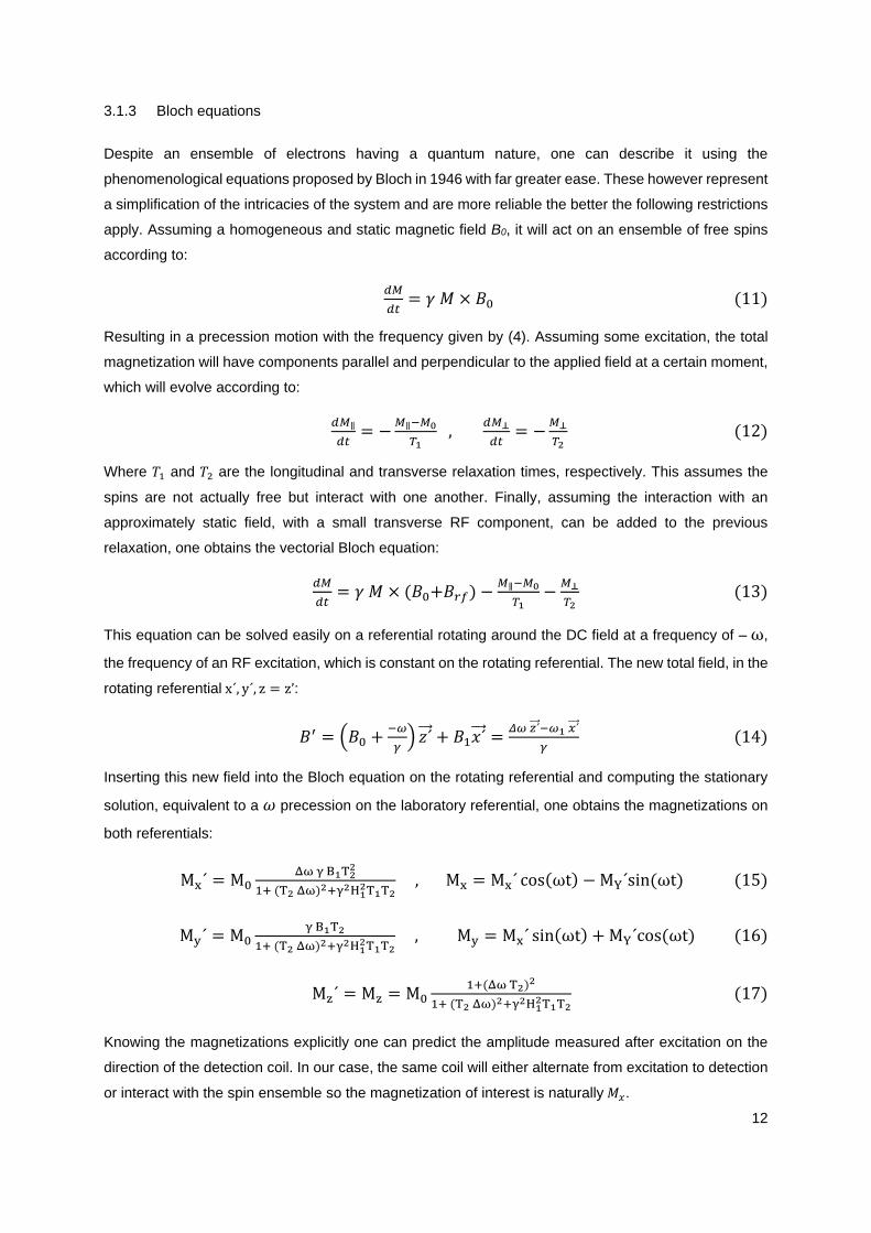
Figure 12 Sine of the nutation angle after 𝜏 ≈ 3 𝜇𝑠 (a) and 𝜏 ≈ 7.5 𝜇𝑠 (b), assuming a 15 mA current,

shown to illustrate the normalized dependence of the signals’ amplitude on the pulse length, according

to equation 43, shown in (c). ................................................................................................................ 23

Figure 13 Full design in exploded isometric view. Dummy models for the PCB’s and microfluidics were

designed to help the dimensioning. Colors shown for clarity: green for PCB’s, orange for adjustment

tables and pink for microfluidics. .......................................................................................................... 24

Figure 14 Isometric (a) and top (b) views of the main holder, in white, the NMR longitudinal holder, in

orange, and of a model for the NMR PCB, in green. Adjusting system is also shown attached to the

moving table. Motion direction indicated by arrows. ............................................................................. 25

Figure 15 Microscrew cap designed, microscrew and its thread and the M6 nut used for attachment to

the system (a). Only a cross section of the piece is shown for simplicity. Example of piece in application,

controlling the distance from the orange wall to the black rotating piece (b). Detail of a pillar for a sliding

part with the locking structures highlighted (c). Motion direction indicated by arrows. ......................... 25

Figure 16 Isometric (a) and top (b) views of the top holder, in white, the EPR longitudinal holder, in

orange, and the transverse holder in white. Adjusting system is also shown attached to the moving table.

Motion direction indicated by arrows. ................................................................................................... 26

Figure 17 Isometric (a), top (b) and back (c) views of the microfluidic holder. The two symmetrical pieces

are shown connected by a locking piece that can be move along the connection. Microscrew cap and

microfluidics model are shown and the holes presented allow locking of the vertical motion on the pillars

through M1.6 screws. ........................................................................................................................... 26

Figure 18 Detail of the holder sliding on the rail and lock-piece system (a) and FEM deformation result

of the normal use of the system (b). The rolling joints shown model the connection of the strained holder

to the rail and lock-piece. The mesh used was constant with squares of 0.1mm in side with deformations

shown in µm. ........................................................................................................................................ 27

Figure 19 Representative images of the results found. Lines with constant deformation, in µm, under a

100kN/m2 stress for the long piece (a) and strain, in absolute value for the same stress, for the small

piece (b). The mesh used was variable going from 2 µm in high strain areas to 50 µm for the long piece

and half for the shorter one. Dimensions shown in mm. All other results are pictured in the appendix.

............................................................................................................................................................. 28

Figure 20 Representation of the piece developed. Picture (a) depicts the use on the setup, clamping

micrometer screw and attached to the holder that moves along the rails, as controlled by the screw.

Following pictures show the FEM meshing and constraints used (b) and a top view of the piece (c). . 29

Figure 21 Deformation (a) and strain (b) results found under stress. Both pictures show the deformed

piece, with a deformation not to scale, and the respective color code and legends. ............................ 29

Figure 5.22 Selected calibration pieces 3D printed for testing. The complimentary male/female pieces

of the rectangular (b) and cylindrical (c) pieces are not shown. Values adapted for STL printer. ........ 30

Figure 23 Final prototype as implemented and used. Detail of the microfluidics (a), of the longitudinal

alignment system (b) and top view of the whole setup on a piece interfacing with the bar inserted into

the magnet (c). ..................................................................................................................................... 31

Figure 24 Detailed microscopic views of the long locking piece under compression until half its length

(a) and under rest (b). On the right (c) a capillary is shown aligned with the center or the coil. Pictures

were color corrected, for clarity, due to the much lower resolution of the camera compared to visual

inspection. ............................................................................................................................................ 31

Figure 25 Evolution of the self-resonating frequency with capacitance for several KEMET RF/microwave

oriented capacitors, for different packages (a). Values taken from the CDR generic official datasheet,

on the left. Characteristic impedance of Texas Instruments capacitors and their advised use in parallel

as stated on the RF operation guideline manual (b). ........................................................................... 32

Figure 26 Design and recommended implementation of the LDO, on the left, input ripple rejection, on

the center and output noise density versus frequency on the right. Values taken from the LP2992 SOIC-

32 datasheet. ....................................................................................................................................... 33

Figure 27 Photograph of the integrated coil (a) and the appended transceiver block circuit (b) as stated

in [42]. .................................................................................................................................................. 33

Figure 28 Spectral noise density figure for a 320 Ω resistor at input, in blue, and for the integrated coil

in red. Downconversion made at 100 MHz, 0 dBm and acquisition at 1.3 MS/s. Picture taken from

published chip documentation [42]. ...................................................................................................... 34

Figure 29 Schematic of the implementation of DC and digital signals on the NMR printed circuit board.

............................................................................................................................................................. 35

Figure 30 Schematic of the AC input stage of the NMR printed circuit board (a). Blocks represent the

Hirose U.FL-R-SMT-1 connectors shown in (b) with its R-134G7210100CD connection cable. .......... 35

Figure 31 Noise density, on the left, and possible gain and phase with frequency, on the right, for the

used OPAMP. Output signal of the chip, in the 10-100 kHz range. Values taken from the

OPA2211AIDDA OPAMP datasheet. ................................................................................................... 36

Figure 32 Schematic of the implementation of the two-stage output buffer and U.FL connector. ........ 36

Figure 33 Layout of the bottom NMR PCB, topview on top and bottom view below. The top layer in red,

the bottom layer in blue and metallized pads in grey are shown for clarity. Dimensions are 100x10 mm2.

............................................................................................................................................................. 37

Figure 34 On the top it is shown the top NMR PCB on (a) and a schematic of a cross section of the

whole system (b). On the bottom, the critical elements of the PCB’s (except the top EPR PCB) are

overlaid, with the top EPR outline in yellow, bottom NMR in green and top NMR in pink (c). .............. 37

Figure 35 Block diagram of the electronics interfacing with the coil (a) and layout of the microchip (b)

showing the two modes of operation: constant frequency and voltage controlled frequency. Unpublished

design similar to [72]. ........................................................................................................................... 38

Figure 36 Electrical schematic for the main PCB interfacing with the EPR microchip on the raised-level

PCB. ..................................................................................................................................................... 39

Figure 37 OPAMP’s frequency response of the noise and gain reliability, as taken from the technical

datasheet. ............................................................................................................................................ 39

Figure 38 Electrical schematic for the raised-level PCB with the EPR microchip in VCO configuration (a)

and fixed frequency configuration (b). .................................................................................................. 40

Figure 39 Layout of the top PCB for use in VCO configuration, fixed frequency is omitted as it is similar.

It is shown the top view’s schematic (a) and manufactured PCB in top view (b) and bottom view (c).

GND pad for chip placement is highlighted. Dimensions are 20x10 mm2. ........................................... 40

Figure 40 Layout of the bottom PCB showing the top view (a), the bottom view (b) and the built and

assembled version in top view (c). The top layer in red, the bottom layer in blue and metallized pads in

grey are shown for clarity. Dimensions are 100x10 mm2. .................................................................... 40

Figure 41 Final implementations of the electrical parts as assembled on the main setup. NMR PCB in

top view (a), EPR PCB in side view (b) and full design being introduced into the magnet (c). In the latter

picture, the modulation coils as well as the Teslameter probe are visible inside the bore of the magnet.

............................................................................................................................................................. 41

Figure 42 Block diagram of the instrumentation required for an NMR experiment. Yellow boxes show

optional components. Other colors shown for simplicity. ..................................................................... 41

Figure 43 Results for a different exponential matched filters on a PDMS signal (a) of a saturating ‘infinite’

sample, at 1T, and for a distilled water sample in the studied capillary in the same conditions (b).

Experimental settings described on the figures. 90º pulses and full relaxation were used (0.5 and 2s

respectively). ........................................................................................................................................ 42

Figure 44 Dependence of the SNR on the output frequency with variable filtering conditions. Comparison

made in the same experimental conditions and optimized filtering conditions. Noise figure present as

background for all experiments at 1 T, for which the operating frequency and corner frequency are

constant. Available corner frequencies and off-resonant excitation dependence shown for clarity. .... 43

Figure 45 Comparison of the results obtained experimentally, through simulation and theoretically, for a

single spin, for variable pulse lengths. Experimental points taken at 7T width a 6.2 kHz off-resonance

excitation and downconversion. Points were averaged 200 times with a 4 s repetition time and a 3 ms

exponential filter. .................................................................................................................................. 44

Figure 46 Block diagram of the instrumentation required for an EPR experiment. Yellow boxes show

optional components/systems. Other colors shown for simplicity. ....................................................... 45

Figure 47 Dependence of the EPR signal on the voltage applied on the modulation coil for magnetic

field sweeps around a 0.7 T field. Sample of approximately 50 mM TEMPO in a 100 µm wide capillary

perfectly aligned with the detection coil (a). Literature obtained results for a 50 mM concentration of

TEMPO (b), as stated in [77]. ............................................................................................................... 45

Figure 48 Frequency output of the EPR chip with variable VCO control voltage (a). Frequency output

and drawn current with voltage across the oscillator’s transistors (b). ................................................. 46

Figure 49 EPR signal for a varying oscillation frequency at a ferromagnet current of 33.5 T, an

approximately 0.7 T field. Sample of 200 mM TEMPO in a 100 µm wide capillary perfectly aligned to the

detection coil. ....................................................................................................................................... 47

Figure 50 Schematic for the alignment procedure of the NMR-DNP setup using a reproducible non-

visual approach. ................................................................................................................................... 48

Figure 51 Saturation dependence on microwave power inside a cavity for different 14N-TEMPOL

concentrations in water for a sample volume of 5 nL measured at 3.4 T (a), taken from [56]. Theoretical

estimates by Armstrong and Han shown as red bars. Enhancement results for 15N-TEMPONE-D in

water, for a 0.35 T field strength, irradiation time from 0.5 to 4s and 6 µL sample volume (b), taken from

[79]. ...................................................................................................................................................... 48

Figure 52 Temperature induced chemical shift changes for H2O/D2O (a) and the reference TMS diluted

in water (b), taken from a standardization of chemical shifts chart [80]. ............................................... 49

Figure 53 Variation of longitudinal relaxation time, DNP build-up time and total enhancement with

temperature for different concentrations of TEMPOL in ethanol. Sample in the µL range measured at

3.4 T showing the results for the CH3 (squares), CH2 (circles) and OH (triangles) peaks. Lines taken

from the expected values for the given concentration as predicted by the dynamic complexation model.

Image taken from [81]. ......................................................................................................................... 49

List of tables

Table 3.1 Gyromagnetic factors and natural abundances of common NMR-visible species ................. 8

Table 2 Electromagnetic and physical constants from the materials used in simulation. Values taken

from literature or simplified to limit cases for ease of computation. All electromagnetic constants are

modeled for 1 MHz and 25ºc. ............................................................................................................... 17

Table 3 Printing limitations obtained from the developed calibration pieces in the in-house STL printer.

............................................................................................................................................................. 30

Table 4 Comparison of 3D printing techniques through their mechanical accuracy and building process.

............................................................................................................................................................. 30

Acronyms

NMR – Nuclear magnetic resonance

EPR – Electron paramagnetic resonance

DNP – Dynamic nuclear polarization

MAS – Magic angle spinning

FID – Free induction decay

OEDNP – Overhauser effect dynamic nuclear

polarization

FEM – Finite element modeling

FWHM – Full width at half maximum

VCO – Voltage controlled oscillator

OPAMP – Operational amplifier

LDO – Low dropout voltage regulator

TEMPO – 2,2,6,6-tetramethyl-1-piperidinyloxyl

PDMS – Polydimethylsiloxane

CMOS – Complementary metal oxide semiconductor

CNC – Computerized numerical control

STL - Stereolithography

MJT – Material jetting

PCB – Printed circuit board

1

1 Introduction

Nuclear magnetic resonance was discovered in 1945 by Felix Bloch1 and Edward Purcell2, for which

both received a Nobel Prize in 1952, and has become an important phenomenon is today’s technological

world. Its widespread application derives from the abundance of sensitive chemical elements and their

observable reaction to a chemical environment all the while being studied in a non-intrusive way. This

ability was proven critical with the increasing use of Magnetic Resonant Imaging machines, for clinical

evaluation of humans and with the precise use of Nuclear Magnetic Resonance spectroscopes to study

highly complex structures like those of proteins. The ability to adjust modularly the components of a

setup, be it the magnetic field amplitude and space and time dependences or the detection mechanism

has widened the spectra of possible uses far beyond the initially envisaged ones. These range from

microcoils attached to chirurgical instruments for image guided surgery to earth-field NMR used in

boreholes drilled for oil extraction. On the other hand, the low sensitivity of the NMR process, due to the

low magnetization of the nuclear spins, along with the existence of this billion dollar market led to the

development of enhancement methods. Through these one can reduce the magnetic fields involved,

and therefore the cost of the required instrumentation, or reduce the time required for signal averaging

until a certain result is viable.

The hyperpolarization method presented in this document is Dynamic Nuclear Polarization, a cross-

polarization between the electrons and the nucleons, has been used from the 1950’s onwards3s and

has achieved enhancements of two to three orders of magnitude. The study and excitation of the

electron spin was achieved through an electron paramagnetic resonance system, to which only a

reduced part of this work will be dedicated, as its main purpose, apart from the crucial excitation, was a

redundancy check and system optimization.

This body of work is divided in three main groups: a brief theoretical background and state of the art,

the detailed fabrication of the setup and the discussion of the results obtained. Initially a wide review of

the state of the art will be presented, focusing on the technical and phenomenological comparison of

several techniques of NMR, followed by a specific view on DNP and more specifically Overhauser DNP.

This will naturally be followed by the theoretical framework of NMR and EPR, due to their formal

similarities, and posteriorly by the theory of the cross-polarization of liquids and solids through dynamic

nuclear polarization. The theory shown is motivated by, and therefore restricted to, the necessary

knowledge to understand and extrapolate from the experiments done. Afterwards, as part of the results

obtained, the magnetic fields’ simulation, is shown. This allows for the understanding of the setup and

its limitations under the light of the previous theoretical considerations. The mechanical and electrical

design of the setup follows up with the most important concepts of the design, with the detailed technical

description of the work being presented as an annex. The microchip architecture is presented alongside

this, despite having been already developed and directly used. Finally, a section is dedicated to the

presentation and discussion of the results obtained and several extrapolations are made, accounting for

the limitations present and the future path to overcome these.

2

2 State of the art

2.1 Magnetic resonance imaging

Nuclear magnetic resonance has seen decades of intense development due to its status as the central

effect on many technologies roughly divided in spectroscopic and imaging techniques.

A certainly principal field in NMR is that of imaging as first proposed by Lauterbur, which managed a 1H

cross-section of two water-filled tubes in 19724. This immediately led to a burst in magnetic resonance

imaging, with the study of increasingly larger parts of the human body and test durations lasting several

hours5. One could spatially define the human body using specialized coils to produce field gradients in

several directions allowing for a varying stationary 𝐵0 field. The procedure varied significantly among

research groups but usually amounted to a linear or planar scan of the area of interest. The most

significant developments came from both field increases, new pulse procedures and complimentary

techniques.

Superconducting magnets are routinely used in MRI but the field’s limitations come not from field

strength but from its homogeneity and drift and the immense stresses supported by the coils, which

must have a bore large enough to insert a human body. The state of the art research for clinical MRI

has made advances towards a 11.75 T magnet with a 900 mm bore and a 0.05 ppm/h drift6. Due to the

immediate correlation between the field gradients and the resolution of the MRI scan, significant

improvements have been made to produce clean gradients across what have become mostly local-

inspection studies. Combinations of different elements, from strips to coils, allow for the local

modification of the field in more precise way leading, for example, to a resolution in cardiac MRI of

1.1x1.1x2.5 mm3 for a 7 T magnet and 32 controllable local active-shimming elements7.

Pulse sequences have been a subject of significant research and are now vast and sufficiently diverse

to adapt to different materials and contrast requirements. A T2-weighed image of a tissue sample, for

example, will show similarly bright results for fatty tissues and for the presence of liquids, giving no

contrast. One the other hand, a T1-weighed image, will show fat as a bright spot and the water in liquids

as dark, being in this case the more appropriate technique. The complex choice of pulse sequences

constitutes a science in itself, weighting test speed, accuracy, sample characteristics and artifact

avoidance to produce the most adequate result and will thus not be further elaborated on, as there are

several compilations on it8.

Lastly, technology is on the brink of enabling NMR microscopy at small sub-micrometric scales, a long

way from the first micro-imaging experiment of a single 1 mm3 cell in 19869. Very recently have high-

precision methods managed to image a single cell with a resolution of 3.7x3.3x3.3 µm3, clearly showing

arrays of sub-cellular components, but required a strict experimental procedure, specific samples and a

long acquisition time10. For clinical applications, ex-vivo on a patient’s skin, a planar scan achieved a

resolution of 25x25x100 µm3, setting a proof of principle for real-time, non-intrusive biopsies on a

patient11.

3

2.2 NMR spectroscopy

2.2.1 Advances and enhancement techniques

On the other hand, and more relevant for this work, is the field of spectroscopic NMR. It has seen

tremendous advance from an interaction point of view, with new ways to hyperpolarize and excite a

sample, as well as from the technological point of view, with better magnets, detectors and cryostats.

Most simply, breakthroughs have come from increases in magnetic field strength, with magnets reaching

45 T in the National High Magnetic Field Laboratory, MagLab12, in Tallahassee, USA and 23.5 T for

commercially available systems at cryogenic temperatures and large bore apertures13. These contrast

with the slowly moving evolution of magnet strengths which went from resistive magnets, topped at the

saturation magnetization of the core’s ferrous material of around 2 T, to superconducting magnets.

They were proposed upon the discovery of superconductivity in 1911 but could only be realized when

superconductive materials were first fabricated. Starting in 1955 with a newly discovered neobium wire

and a generated field of 0.7 T at 4.2 K14, these magnets evolved to allow for supercurrents and to be

used at high temperatures, allowing for the use of Nitrogen instead of liquid Helium, as in the case of

the pioneering Yttrium barium copper oxide, YBCO, which managed a field of 26.8 T in 198715.

Developments in pulsed magnets, despite requiring different experimental conditions and lacking the

same averaging abilities, have had very significant achievements with MagLab reaching pulses of 100

T for 25 ms at 400 mK and even 300 T for 5 µs at 4.2K. Concurrently, magnets supporting cryogenic

deep temperatures have also been developed with MagLab achieving a continuous field of 21 T at a

few µK.

Conversely, recent advances have allowed for the progress made in the field of very-low field NMR,

namely at the earth’s magnetic field of 30-60 µT (EFNMR), ever since it was first used in spectroscopy

and imaging16. The use of such a field, with usual polarizations of only a few ppb and where chemical

shifts are much less significant than J-couplings, has the advantage of a naturally high homogeneity and

the use of big samples. It manages to achieve the longest FID through the matching of T2−1 = T2

∗−1

usually differing by a significant factor proportional to the field inhomogeneity. The long averaging times

are diminished through the use of hyperpolarization techniques on the sample. In this strong coupling

regime, chemical shifts of several known molecules, at a linewidth of ~0.1Hz, have been distinguished

using only a 2T pre-polarizing setup17 with agents that J-couple to the sample therefore resolving the

overlapped lines. This regime presents the most complex spectra but allows for an easily portable

alternative to superconducting magnets.

Several techniques have been developed to avoid line broadening, allowing for the visualization of J

couplings, critical for chemical identification, through the homogenization of the effective field seen by

the nucleons. This is achieved using shimming techniques, to avoid field inhomogeneity and angle

averaging techniques, namely magic angle spinning (MAS).

4

Shimming, the processes of reducing B0 field inhomogeneity is a cornerstone of any NMR/MRI test, as

any broadening of a line will hide chemical information and decrease the signal amplitude, which is

inversely proportional to the width of a peak. These have been applied using geometrically symmetrical

coils to apply field gradients across the three axes after, for example, field-inhomogeneity mapping

through field pulses18. It is possible to eliminate first-order deviations, a common problem for in-vivo

MRI, and even use localized coils to perfect the field in one area to the detriment of adjacent areas19.

The localized analysis in a contained environment, as that of a commercial NMR magnet, usually doesn’t

require such a critical field correction but instead the correct placing of a sample inside the bore magnet.

Mechanical adjustments of the sample holder usually correct the position through a feedback loop based

on the lack of symmetry and height of the Lorentzian lineshape20. Using a 5th order shim set and an

alignment system field inhomogeneity has been proven to be reducible by over an order of magnitude.

This reduction would lead to a vertical ~2 ppb inhomogeneity in a 500 MHz spectrometer with a sample

with sub-millimeter width inside a saddle coil with susceptibility correction and a subsequent linewidth

of 0.36 Hz21 (due to radial inhomogeneity). Experimentally achieved linewidth in the aforementioned

conditions was of 2.2 Hz.

Complementarily, MAS has allowed for high-resolution solid state NMR spectroscopy, with linewidth

reaching the sub-Hertz regime which contrasts with the natural linewidth of a few kHz. Decomposing

spin interactions in spherical harmonics one can see that angular contributions can be averaged out

through rotation around an axis. Dipolar interactions can be fully averaged out through the rotation about

the magic angle, cos−1 (1

√3) , and chemical shift anisotropy, quadrupolar interaction and nuclear-electron

interactions can be partially averaged out. This justifies the finite linewidth of MAS sharpened samples

and for better improvement, cancelling higher order interactions, one would have to simultaneously

rotate the sample across other axes, which poses an increasingly complex setup due to the speed at

which they must be rotated of some kHz, the peak linewidth22. This was achieved using double rotors

(DOR-NMR) thus averaging out the second order quadrupolar broadening characteristic of spin 3/2

nuclei, such as 17O, as soon as 198923.

On the other hand using MAS removes dipolar information, whose high distance sensitivity is a critical

parameter in molecular structure studies. This has nonetheless been solved through a novel pulse

sequence which gave rise to the technique of dipolar recoupling24, which can be used along with MAS.

Another immediate limitation is that of mechanical and thermal constraints. Large samples require

equally large rotors and holders and induce great stresses on the material thus forcing a reduction of

the rotating speed. Furthermore, high speed rotation induces significant heating which makes achieving

cryogenic temperatures hard. A compromise is usually attained with reduced rotating speeds, from the

50 kHz attainable for a 10 µL sample at room temperature, to the same sample in a constantly

refrigerated heat exchanger with a temperature of 7, 13 and 20 K at rotation frequencies of 5, 10 and

20 kHz, respectively25. As an addition to existing systems several commercial probes have been

developed for low temperature MAS at moderate abilities, for example a 3 mm, 20 kHz probe working

at 130 K by Doty ScientificTM.

5

As sensitivity is the main limitation of NMR, due to the very small relative magnetization of the nuclei,

several hyperpolarization techniques have been developed for use in different contexts and are

henceforth compared.

Currently used in chemistry is the effect of Chemically Induced DNP (CIDNP) which is based on the

introduction of an optically excited radical. This starts electron-spin dependent reaction rates for radicals

which induce a cross-polarization on the nucleus of the native species. This effect is thus effectively a

surface effect and it is used not for its enhancement, up to three orders of magnitude26, but for its

chemical selectivity. CIDNP is therefore a more a labelling technique that is fundamentally different from

other hyperpolarization methods27.

Also widespread in chemistry is the technique of Parahydrogen, the singlet spin state of molecular

hydrogen, Induced Polarization (PHIP). Through the manufacture of pure Parahydrogen, from the 25%

that would exist in a room temperature sample of H2, and the mixing of a sample with it exceptional

hyperpolarizations can be achieved. These range up to four orders of magnitude, with the use of a

catalyzer28, the use of the hydrogen itself (e.g. Hydrogenation reactions) or of a mixing pulse sequence

(e.g. SABRE) in a magnetic field. PHIP has found wide applicability in the hyperpolarization of hydrogen

(ε=30027) as well as lower gyromagnetic ratio nuclei (e.g. 13C, ε=400027), both in NMR and MRI.

As a last technique one finds DNP in all its experimental implementations: solution/solid state, high/low

field, dissolution and shuttling.

Shuttling DNP compensates for one limitation of DNP, the low enhancement at high fields. To achieve

the best of both worlds, a sample can be polarized at low field and shuttled to high-field for measurement.

Samples in solution have been polarized at 0.35 T, achieving an enhancement of ≈110 and then

analyzed at 14 T, giving a total enhancement of 15 (considering the reduction from the field ratio)29.

A groundbreaking complement to shuttling is the use of photo-excited electrons to perform the

hyperpolarization, which avoid the maximum 660 enhancement restriction of electrons in thermal

equilibrium30. Using pentacene-d14 as a polarizing agent, photoexcited to the triplet state by a laser, a

34% polarization of 1H was achieved, which corresponds to an enhancement of 250 000 relative to room

temperature polarization .

Dissolution DNP has also found wide applicability, being used to hyperpolarize samples, contrasts for

MRI and radicals for cross polarization all in solution state. It was initially developed as a sample shuttled

from a low-field magnet where hyperpolarization would be achieved, through microwave irradiation at

cryogenic temperatures, to a high-field NMR magnet. The sample is quickly shuttled and warmed up

before being analyzed thus maintaining its polarization and was proven to have an enhancement of

44000 and 23500 for 13C and 15N, respectively31. Two interesting complementary developments are the

solution to the downside of long polarization build-up times, through the cross polarization of low-gamma

nuclei from Hydrogen32 for example (as T1H<<T13C), and the loss of polarization during shuttling, reduced

for Hydrogen long lived states whose T1 was initially increased33 up to a factor of 7 to recent increases34

in 13C’s T1 of up to 50.

6

2.2.2 Mass-limited spectroscopy

Mass-limited NMR may prove to be an important tool in the future as it’s limited sample may be all that

is available, for example in the beginning stages of the infection of HIV. The volume of the required

mass has been slowly declining, due to the harsh dependence of the SNR on the sample’s spins, going

from the first attempt at reduced size RF microcoils made for CW-NMR in 1966 at a volume of a few

µL35 , to 5 nL in 199836 to the attempt at a sub-nanoliter sample in this work. Such a sample would

encompass a cube with only tens of micrometers in size, the dimension of most animal and plant cells,

and could possibly allow for unprecedented non-invasive studies on the building blocks of life. Currently

this would only be achievable in acceptable time windows for high density compounds, an ability

matched for example by state of the art fluorescence studies37, but with increasing sensitivity the

discretization of cellular components, such as the 10 µm wide nucleus, might be chemically analyzed in

real-time as they develop and interact. This technique requires however a departure from normal

methods in NMR due to the peculiarities of a microcoil and the required electronics, on which the usually

negligible effects of susceptibility mismatches or parasitic capacitances become relevant, for example.

Initially, an advantage with small samples is their reduced vulnerability to field macroscopic

inhomogeneity but increased to susceptibility mismatches due to the small distances to the coil. These

have significantly reduced the necessity of morose active shimming procedures but still use the same

setups to achieve the best possible positioning and linewidth38. Susceptibility-related broadening may

be avoided using either susceptibility matching fluids/containers, a process called passive shimming, or

for smaller designs a careful finite element simulation of a microfabricated coil39. A proven technique,

which resulted in significant ease of handling, is that introduced by Behnia in 199840 of using same-

susceptibility immiscible fluids on the same capillary to plug the relevant sample instead of using a larger

sample and referring to the sample volume as only that which is inside the sensitive volume.

Another aspect if that of the size and quality of the coil, which directly affect the filling factor, the ratio of

sample to sensitive volume, and the sensitivity of the coil, B(i)/i, to which the signal-to-noise ratio is

proportional. One must thus reduce the size of the coil to fit the sample, knowing the signal will be

proportional to the number of spins and hence the sensitive volume. Furthermore, one would ideally

construct a resonant coil to exploit the intrinsic gain given by it while staying below the self-resonant

frequency, but this doesn’t always prove possible.

Several microcoil geometries have been implemented, namely stripline, planar and solenoidal.

Regarding planar coils, a low-field resonant design was achieved for Q=7.2 at 28 MHz and a 120 µm

radius41 and several non-resonant ones have been used with few surpassing the ~50 µm mark due to

sensitivity limitations42. These have the notorious advantage of being able to be assembled in arrays,

either for multiple simultaneous analysis or imaging, but have been limited to larger sizes, usually a

radius of 0.343 to 211 mm. Fabrication of the aforementioned planar microcoils was achieved either

through microfabrication, with several steps using lithography on PDMS and copper electroplating44, or

through metallized areas on the already established CMOS process, allowing for seamless integration

with the electronics42.

7

Micro-solenoids, due to their use in the MEMS industry, have achieved relatively small dimensions and

high quality factors, along with their intrinsic high B1 field uniformity, but small usage in NMR due to the

difficulty of miniaturization, parallelization and sample insertion. These have achieved high-Q designs

with 1 mm wide solenoids with tens of windings at a pitch of 40 µm and a field uniformity up to 3%45,46

and, for highly reduced samples, at a proton frequency of 500 MHz, an array of solenoids with a diameter

of 370 µm47. Fabrication methods are more complicated than for planar coils and require moving

substrates which adapt their orientation to the direction of deposition or to the wire-bonding tip45 that is

usually used.

Finally stripline designs, a novel geometry introduced for NMR in 200748, have broken ground for a

scalable design, to sub-micrometric dimensions, in one simple lithographic process. These allow for a

zero-distance to the sample, for parallelization and a highly homogenous excitation field without ever

introducing susceptibility mismatches. These have been optimized as a single stripline attaining a

linewidth of 0.7 Hz and a spin sensitivity of 1014 at dimensions of hundreds of micrometers49.

Several other designs, such as saddle, Helmholtz or double helix have been introduced to shape the

field or allow for cooling, for example, but all were made in the millimeter range50,51 due to the difficulty

of micromachining complex geometries at the micrometric scale.

One other side of mass-limited analysis is that of integrated sample handling and containment. Test

tubes to hold samples become small glass capillaries in the micrometric regime, with 25 µm wide glass

capillaries with 12 µm walls and variable cross-section shapes being available commercially and smaller

ones being achieved through microfabrication. The study of a system with several organic compounds

is often prohibitively complex and hard to achieve, due to the low concentration of each species. Thus

have micro-separation techniques proven useful when using small samples in a capillary, usually as

part of a micro total analysis system (µTAS). The most common ones52 are electrophoretic separation

through capillary electrophoresis (CE) or capillary isotachophoresis (cITP) and capillary liquid

chomatography (cap-LC). The use of on-line separation using a continuous flow through an

electromagnetic field, which is alternated with NMR acquisition so as not induce line broadening, has

managed to increase concentrations up to 2 or 3 orders of magnitude, depending on the compound53.

General figures of merit for mass-limited spectroscopy, like spin sensitivity, are usually hard to state due

to the independent variation of time expenditure, spin concentration and dimensions used across state

of the art devices as well as the author’s definition of limit of detection. The NMR microchip used in this

project achieved a spin sensitivity of 1.5 × 1013 spins/√Hz42 and single stripline detectors have achieved

2.8 × 1014 spins/√Hz49, for example. Hyperpolarization of mass-limited samples has not been widely

studied but, so far, dissolution DNP enhancements of ≈500, for 1H, were achieved at 3.4 T for 10 nL

samples with 5s repetition times54. Relaxation losses, saturation dependencies55 and temperature

effects have also been studied in the nanoliter regime at smaller enhancement factors, obtaining for

liquid-state high-field DNP results not predicted by Overhauser theory56.

8

3 Theoretical framework

3.1 Magnetic resonance

3.1.1 Magnetism

The phenomena of the resonant excitation of a spin is the physical basis of both nuclear magnetic

resonance and electron paramagnetic resonance, the difference being the respective interaction with

the nuclear and electron spins57. These are usually studied separately as the significant difference in

energy splittings infers a physical independence of both processes with the instrumentation and

methods used being radically different. Initially, the basis for these effects will be presented with special

attention to parallelisms and differences in the theory of NMR and EPR. Despite spin being an

intrinsically quantum characteristic its nature and dynamics can be treated classically or semi-classically

for the purpose of the work done.

The phenomena of NMR, consists on the interaction with the spins of the nucleons when the total nuclear

spin is different from zero. As the spin number of each nucleon is ½, the total nuclear spin will be

proportional to a half integer I = ℏm = 0,ℏ

2, ℏ… , where ℏ is the reduced Planck constant and 𝑚 is the

magnetic quantum number.

This occurs mostly when there is an odd number of protons or neutrons, as for an even number the

nucleons would pair up in the lowest energy orbitals with anti-parallel spin states and hence the total

nuclear spin would equal zero. The exception consists of degenerate nuclear orbitals which allow for

several spin-parallel states. These two cases represent the extreme cases of 12C and 16O, which have

I = 0 and no NMR spectra and of 10B with m = −3,−2,−1, 0, +1,+2,+3 and a subsequently much more

elaborate spectra.

Being a vector quantity, the spin angular momentum will be proportional to the scalar spin and will

consequently have, in a magnetic flux density B , a proportional energy:

𝜇 = 𝛾 𝐼 , 𝐸 = − 𝜇 . = −𝛾 𝐼. (1)

where 𝛾 is the gyromagnetic factor of the nucleus and the energy splitting is usually referred to as the

Zeeman energy.

Table 3.1 Gyromagnetic factors and natural abundances of common NMR-visible species

Species 1H 2H 13C 14N 15N 17O 29SI 31P

γ (MHz/T) 42.5 6.54 10.71 3.077 -4.316 5.77 -8.47 17.24

Natural

abundance

(%)

99.985 0.015 1.108 99.63 0.37 0.037 4.7 100

9

Unlike how the response of nuclear spins is highly dependent on the atomic number, the electron

gyromagnetic ratio does not vary much within paramagnetic samples, with g-factors usually ranging

within 20% of the normal value of ≈2, which gives a free electron γe = 28.0250 GHz/T. This justifies the

more universal nature of EPR systems whereas NMR spectrometers are targeted to the interaction with

a specific element nucleus, usually 1H or 13C for their biological availability.

In a strong magnetic field the spins will have a preferential alignment along the magnetic field to minimize

the energy. Assuming an approximately Boltzmann-like energy occupation with energy, one may

compute the variation of the normalized net magnetization, the polarization 𝑃, for nuclei with spin 𝐼:

𝑃 =∑ 𝑚 𝑒

𝛾ℏ𝑚𝐵𝑘𝑇𝐼

−𝐼

∑ 𝑒𝛾ℏ𝑚𝐵

𝑘𝑇𝐼−𝐼

≈𝛾ℏ 𝐼 (𝐼+1)

3𝑘𝑇𝐵 , 𝛾ℏ𝑚𝐵 ≪ 𝑘𝑇 (2)

where one can observe the Curie-like 1/T dependence and a linearity with the magnetic field when

approximating the exponential in the high-temperature regime, as the thermal energy at 300K, 25meV,

is much larger than the Zeeman splitting, which is inferior to a µeV for current field strengths of a few

Teslas.

For a two-state system, alike that of electrons, on can statistically show the polarization to be as follows,

considering the same Boltzmann level occupation, which reduces to (3) at small magnetic energies

relative to the thermal energy and for I = S = 1/2:

𝑃 = 𝑡𝑎𝑛ℎ (𝛾ℏ𝐵

2𝑘𝑇) (3)

Figure 1 Theoretical polarization of electrons and protons at different fields with a variation in temperature, according to equations (2) and (3). Image taken from ‘Nuclear Magnetic Resonance58’.

It is the disparity shown in Fig.1 that led to the development of cross-polarization techniques,

hyperpolarizing protons up to the polarization of the electrons at the same field, an enhancement of up

to γe

γn⁄ , equaling ≈660 for Hydrogen and ≈2625 for Carbon. All these considerations are applicable to

a system in thermal equilibrium, as excited systems require a more complex treatment but allow for

much higher enhancements.

10

3.1.2 Spectroscopy

Much can be said on the interpretation of NMR spectra but this work will briefly go over the four main

internal responses to an applied magnetic field: chemical shifts, dipolar and quadrupolar coupling and

scalar coupling.

Any free spin under the influence of a static magnetic field will precess around that same field at the

Larmor angular frequency ω:

𝜔 = 𝛾𝐵 (4)

However, the nucleus’ electrons will react to the field either paramagnetically or diamagnetically thus

deshielding or shielding the external magnetic field, respectively, which gives rise to shifted frequencies

that depend on the specific chemical environment of each species:

𝜈 =𝛾𝐵0(1−𝜎)

2𝜋 (5)

Where σ is the screening constant, for each shift, from which one can define a field-independent

chemical shift, scaled to ppm:

𝛿 = 106 (𝜈−𝜈𝑟𝑒𝑓)

𝜈𝑟𝑒𝑓= 106

(𝜎𝑟𝑒𝑓−𝜎)

1−𝜎𝑟𝑒𝑓≈ 106(𝜎𝑟𝑒𝑓 − 𝜎) , 𝜎𝑟𝑒𝑓 ≪ 1 (6)

The reference can be varied, as it introduces only a constant shift, but is usually taken for hydrogen and

carbon NMR as TMS, (CH3)4Si, due to its strong signal and ease of use. This has proven to be an

important method to determine the structure of compounds as the shifts are not field dependent and

provide insights into the chemical environment of each nucleon.

Scalar coupling, or indirect dipole-dipole coupling, is an effect between nuclear spins mediated by

intermediate electrons. This usually, but not necessarily always, occurs when a covalent bond exists

between two atoms with s-valence orbitals. This is because the spins are related through the Fermi

contact interaction, which is an interaction only appreciable at very small distances:

ℋ𝐹𝑒𝑟𝑚𝑖 ∝ −𝛾𝑒 𝛾𝑛 < 𝐼. 𝑆 > |𝛹(𝑟 = 0)|2 (7)

From which one can deduce that only s-orbitals will have a non-zero value at the nucleus. It should be

noted that for energy minimization, as the electron has a negative gyromagnetic ratio, the nuclear and

electron spins should be antiparallel. One can therefore simplify the interaction through:

ℋ𝑠𝑐𝑎𝑙𝑎𝑟 = −𝐼𝑖 ∑ 𝐽𝑘𝑖𝑘 𝐼𝑘 (8)

With the coupling constant J for the kth nuclei usually being around 100 Hz. One can see that magnetically

equivalent nuclei will have the same coupling constant and the splitting will depend only on the

configuration possibilities. Hence, for a common AXi configuration like that of CH4, the multiplicity of the

kth peak will be given by the kth entry of the ith row of the Pascal triangle, or (ik), as exemplified on the

real spectrum shown in Fig.2.

11

Figure 2 400MHz 1H NMR spectra of ethanol showing the different H chemical environments and the scalar splittings of 1:3:3:1 and 1:2:1 for AX3 and AX2 groups, respectively. The splitting for CH2 is comes from the coupling to the CH3 group, not itself, due to its magnetic equivalence. Image taken from ‘Nuclear Magnetic Resonance58’.

Furthermore, one can have the direct coupling in-between the spin magnetic moments of the two

nucleuses in what is known as dipolar coupling. This reduces to the dipolar magnetic field of one of the

spin acting on the other, separated by r 12, resulting on the following Hamiltonian:

ℋ𝐷12 = −𝜇2 .(3(𝜇1 .𝑟12 ) 𝑟12

|𝑟12|2−𝜇1 )

|𝑟12|3 (9)

The Hamiltonian’s angular dependence is rather complicated but retains, to first order, a simple

dependence of [1 − 3 cos2(θ)]|r12|−3 and it is, due to its sharp distance dependence, a good

measurement of inter-nuclear distances. This field independent characteristic is usually of up to a few

kHz in energy.

Finally, one can have the quadrupolar coupling characteristic of nuclei of spin >½. This broadening

effect, leading to characteristic lines, is caused by a charge inhomogeneity within the nucleus induced

by an external electric field gradient. Because of its naturally complex description it can be simplified

using the experimental quantities η, the axial electronic symmetry of the system relative to the strongest

electric field gradient as the axis z (e.g. η=0 for pz orbital), q the average axial potential per unit charge

and Q the quadrupole moment tensor of the nucleus:

ℋQ =e2Qq

4I(2I−1)[3Iz

2 − I(I + 1) +1

2η(I+

2 + I−2)] (10)

With the quadrupole coupling constant clearly shown as χ =e2Qq

4I(2I−1). This broadening will not be present

on the experiment done as it is made for a spin ½ but when present can induce incredible broadenings

up to the megahertz range due to quick relaxation effects. The anisotropy of chemical shifts and the

couplings presented can induce a significant broadening of the spectral lines, possibly masking certain

features. This can however be avoided/reduced through the averaging of the interaction, as they show

a clear angular dependence, which can be achieved both naturally, through the molecular tumbling in a

liquid solution, or through forced rotation as is the case of magic angle spinning. Quadrupolar

broadening shows the same [1 − 3 cos2(θ)] dependence on the first order correction to the energy but

a sin2(θ) cos (2ϕ) dependence as second order, meaning it cannot be averaged with single-axis

rotation.

12

3.1.3 Bloch equations

Despite an ensemble of electrons having a quantum nature, one can describe it using the

phenomenological equations proposed by Bloch in 1946 with far greater ease. These however represent

a simplification of the intricacies of the system and are more reliable the better the following restrictions

apply. Assuming a homogeneous and static magnetic field B0, it will act on an ensemble of free spins

according to:

𝑑𝑀

𝑑𝑡= 𝛾 𝑀 × 𝐵0 (11)

Resulting in a precession motion with the frequency given by (4). Assuming some excitation, the total

magnetization will have components parallel and perpendicular to the applied field at a certain moment,

which will evolve according to:

𝑑𝑀∥

𝑑𝑡= −

𝑀∥−𝑀0

𝑇1 ,

𝑑𝑀⊥

𝑑𝑡= −

𝑀⊥

𝑇2 (12)

Where 𝑇1 and 𝑇2 are the longitudinal and transverse relaxation times, respectively. This assumes the

spins are not actually free but interact with one another. Finally, assuming the interaction with an

approximately static field, with a small transverse RF component, can be added to the previous

relaxation, one obtains the vectorial Bloch equation:

𝑑𝑀

𝑑𝑡= 𝛾 𝑀 × (𝐵0+𝐵𝑟𝑓) −

𝑀∥−𝑀0

𝑇1−

𝑀⊥

𝑇2 (13)

This equation can be solved easily on a referential rotating around the DC field at a frequency of – ω,

the frequency of an RF excitation, which is constant on the rotating referential. The new total field, in the

rotating referential x´, y´, z = z’:

𝐵′ = (𝐵0 +−𝜔

𝛾) 𝑧´ + 𝐵1𝑥´ =

𝛥𝜔 𝑧´ −𝜔1 𝑥´

𝛾 (14)

Inserting this new field into the Bloch equation on the rotating referential and computing the stationary

solution, equivalent to a 𝜔 precession on the laboratory referential, one obtains the magnetizations on

both referentials:

Mx´ = M0Δω γ B1T2

2

1+ (T2 Δω)2+γ2H12T1T2

, Mx = Mx´ cos(ωt) − MY´sin (ωt) (15)

My´ = M0γ B1T2

1+ (T2 Δω)2+γ2H12T1T2

, My = Mx´ sin(ωt) + MY´cos (ωt) (16)

Mz´ = Mz = M01+(Δω T2)

2

1+ (T2 Δω)2+γ2H12T1T2

(17)

Knowing the magnetizations explicitly one can predict the amplitude measured after excitation on the

direction of the detection coil. In our case, the same coil will either alternate from excitation to detection

or interact with the spin ensemble so the magnetization of interest is naturally 𝑀𝑥.

13

More explicitly, one can state the problem in a way similar to that of a Fourier transform:

Mx + iMy = (Mx´ + iMy´)eiωt (18)

Meaning the FFT performed during the signal acquisition will immediately return the components on the

rotating referential, with some introduced phase, which justifies the use of such a coordinate change

throughout this section. The previously stated magnetizations at negligible saturation, γ2H12T1T2 ≪ 1,

are reduced to:

𝑀𝑥´ = (𝑀0𝜋 𝛾 𝐵1𝑇2) 𝛥𝜔 𝑓𝑇2(𝛥𝜔), 𝑀𝑦´ = (𝑀0𝜋 𝛾 𝐵1) 𝑓𝑇2

(𝛥𝜔) (19)

Where 𝑓 is a normalized Lorentzian lineshape with an FWHM equal to 𝑇2. Conversely, at significant

saturation, γ2H12T1T2 ≫ 1, the magnetization is reduced by a factor of T2

′/T2 and the lineshape is

broadened to T2′ which behaves as:

𝑇2′ = 𝑇2 (1 + 𝛾2𝐻1

2𝑇1𝑇2)−0.5 (20)

Due to the 90º in-between the x and y magnetizations one can define the following tensor components:

𝜒𝑥𝑥′ =

𝑀𝑥´

2 𝐻1= 𝜒𝑦𝑥

′′ , 𝜒𝑦𝑥′ =

𝑀𝑦´

2 𝐻1= −𝜒𝑥𝑥

′′ (21)

Which allows for the simplification of the measurable magnetic susceptibility for a single coil system,

defined up to an experimental phase as χxx = χxx′ + iχxx

′′ :

𝜒𝑥𝑥 = 𝜒0𝜋

2

𝜔0𝛾 𝐵1𝑇2

1+ (𝑇2 𝛥𝜔)2+𝛾2𝐻1

2𝑇1𝑇2

(−𝑇2 𝛥𝜔+ 𝑖) (22)

This phenomenological approach can be refined to account for a common limitation, the magnetic field’s

inhomogeneity. Creating a normalized quantity of spins around the expected frequency x + H0/γ, ℎ(𝑥),

one can average the behavior of each local Lorentzian, related to a certain field, across the entire

sample:

𝑀𝑥,𝑦´ ∝ 𝑓𝑇2(𝛥𝜔) = ∫ 𝑓𝑇2

(𝛥𝜔 + 𝑥)∞

−∞ℎ(𝑥)𝑑𝑥 (23)

Assuming the linewidth is dominated by field inhomogeneity, ℎ will have a much slower variation with 𝑥

than 𝑓, which will be a sharp peak at x = 0. One can thus approximate the integral as if the peak was a

Dirac delta and therefore obtain:

fT2(Δω) = h(Δω) ≈ f

T2† (Δω) , T2

† = (γ ΔB0)−1 (24)

Where it was assumed that the field distribution was roughly that of a Lorentzian with FWHM equal

to T2†

. Plugging the assumed ℎ into the integral one reobtains:

fT2(Δω) = fT2

∗ (Δω), T2∗ −1 = T2

† −1+ T2

−1 (25)

Which gives an experimentally measurable quantity related to the field inhomogeneity that would be

otherwise hard to measure for small samples spaces.

14

3.2 Dynamic nuclear polarization

3.2.1 DNP mechanisms

Dynamic nuclear polarization is one of the many hyperpolarization techniques available today and relies

on the transfer of polarization from electrons to nucleons through double flips59. The process is initiated

through some means of polarizing the electrons: a chemical reaction, as in the case of chemically

induced DNP (CIDNP), through spin injection or the most common, optical pumping. Microwave driven

DNP has become widespread with the advent of suitable sources such as gyrotrons and is divided in

four cross-polarization transfer mechanisms: the Overhauser effect (OE), the cross effect (CE), the solid

effect (SE) and thermal mixing (TM). So far, only the Overhauser effect has been observed in liquids

with the other effects being observed for solid state (SSDNP) samples, hence OEDNP having a detailed

description in the upcoming section.

CE, SE and TM DNP are based on anisotropic interactions and are directly triggered after microwave

irradiation meaning they are not suitable for liquid DNP due to translational averaging.

The SE relies on the hyperfine coupling between a nucleus and an electron which creates ‘forbidden’

Double-Quantum (DQ, e.g. αα → ββ) and Zero Quantum (ZQ, e.g. αβ → βα) transitions that

simultaneously flip the electron and the nuclear spins. Naturally the irradiated frequency must match the

energy difference of the transitions, ωe ± ωn, thus for a concentration 𝑁𝑒 the enhancement is,:

εSE ∝γe

γn(B1e

B0)2 Ne

δT1e (26)

Where the EPR homogeneous linewidth δ and inhomogeneous linewidth Δ must be smaller than the

nuclear frequency and a B0−2 dependency is clear.

The CE effect, on the other hand, uses the dipole-dipole coupling between two electrons hyperfinely

coupled to a nucleus. The mechanism is similar to SE, the difference being that the incoming radiation

polarizes an electron that will then induce the flip of the other electron and the nucleus if ωe1 − ωe2 =

ωn. The radiation used must therefore have a frequency ωe1 or ωe2 and the enhancement is ∝ B0−1 for:

εCE ∝γe

γn(B1e

2

B0) (

Ne

δ)2T1e (27)

For this mechanism the condition δ < ωn < Δ must be fulfilled, which strongly correlates to the density

of the polarizing agent and its dipolar induced broadening. The less constraining field dependence led

to CE being the main effect seen in high-field DNP.

Finally, TM is a mechanism qualitatively similar to that of CE with a different theoretical approach, based

on the concept of spin temperature, and thus the field dependence is the same, B0−1. Its predominance

at very high radical concentrations requires the statistical treatment of an ensemble of electrons due to

the high dipolar couplings.

15

3.2.2 Liquid-solid OEDNP

Liquid state DNP has its own peculiarities which require different methods to overcome, but presents

several benefits over SSDNP. It has become divided in same-field and shuttling DNP27. To perform a

viable microwave excitation in an NMR spectrometer for same-field DNP, one should have an optical

setup attached to perform high quality EPR or avoid this through the use of continuous flow or shuttling

techniques. Polarizing a sample at a lower field EPR spectrometer or at a much lower temperature, a in

the case of dissolution DNP (D-DNP), and quickly shuttling it to the main NMR spectrometer, one can

easily adapt two high quality devices for a relative enhancement that accounts for the losses from

relaxation in the different i sites:

ε

ε0=

TNMR

TEPR

BEPR

BNMR∏ e−ti/Ti

i (28)

During initial considerations on this work, a similar shuttling application was considered, however this

carried an implicit enhancement loss. This option was kept as a backup solution as the reduced size of

the excitation chips allowed for a simultaneous use without enhancement loss, provided the alignment

was adequate. This will allow for the use of a setup, as a future step, on a high-field NMR magnet,

without the field loss factor and at cryogenic temperatures.

The Overhauser effect relies on a saturation of the electron transition, whose frequency the irradiated

frequency must match, and the subsequent relaxation from that excited state. For a system with cross-

relaxation and auto-relaxations rates 𝜎 and 𝜌, respectively:

d⟨Iz⟩

dt= −ρ(⟨Iz⟩ − I0) − σ(⟨Sz⟩ − S0) (29)

Figure 3 Energy levels of the electron-nucleus system with respect to spin orientation. Zero-quantum, W0, single quantum, W1S and W1I, and double-quantum, W2, spin transitions are shown. Image taken from ‘Dynamic nuclear polarization in liquids’ 59.

The rate equation (29) can be simplified to more experimentally measurable factors such as the

saturation factor 𝑠, the leakage factor 𝑓 and the coupling factor 𝜉:

𝑠 =𝑆0−⟨𝑆𝑧⟩

𝑆0 (30), 𝜉 = 𝜎

𝜌=

𝑊2−𝑊0

𝑊0+2𝑊1+𝑊2 (31), 𝑓 =

𝜌

𝜌+𝑊1𝐼 (32)

16

For which the expression of the enhancement can be simplified to:

휀 =⟨𝐼𝑧⟩

𝐼0= 1 − 𝑠 𝜉 𝑓

|𝛾𝑒|

𝛾𝑛 (33)

As the maximum possible enhancement runs according to 휀 = 1 − 𝜉 |𝛾𝑒|

𝛾𝑛, it will therefore be scaled

according to interaction mechanisms and very significantly with the used compound. Global

hyperpolarization comes however from the hyperfinely coupled electron/nucleus pair of the coupled

radical molecule that usually polarizes hundreds to thousands of neighboring nuclei. As such, spin

diffusion must play a central role on the overall enhancement of the signal and it has been shown to

come from nuclear-dipolar interactions in solid state DNP60. Cross and self-relaxation in OEDNP have

been semi-classically computed by Hauser61 for scalar and dipolar mechanisms as:

𝜌𝑆 = −𝜎𝑆 =𝐴2

2𝑓𝜏𝑠2(𝜔𝑛 − 𝜔𝑒) + 𝛽𝑓𝜏𝑠1(𝜔𝑛) (34)

𝜌𝐷 =𝛾𝑛

2𝛾𝑒2ℎ2

10 𝑟𝑒𝑛6 [6𝑓𝜏𝐷(𝜔𝑛 + 𝜔𝑒)−𝑓𝜏𝐷(𝜔𝑛 − 𝜔𝑒) + 3𝑓𝜏𝐷(𝜔𝑛)] (35)

𝜎𝐷=𝛾𝑛

2𝛾𝑒2ℎ2

10 𝑟𝑒𝑛6 [6𝑓𝜏𝐷(𝜔𝑛 + 𝜔𝑒)−𝑓𝜏𝐷(𝜔𝑛 − 𝜔𝑒)] (36)

Where it was considered 𝜏𝑆1,2−1 = 𝜏1,2

−1 + 𝜏𝑒−1 and 𝜏𝐷

−1 = 𝜏𝑒−1 + 𝜏𝑟

−1. The coefficient 𝛽 was introduced to

account for the time dependence of scalar relaxation by spin exchange. Thus 𝛽 will range from 0 for

𝜏𝑒 ≪ 𝜏1, 𝜏2 to 1 for 𝜏𝑒 ≫ 𝜏1, 𝜏2. The type of relaxation mechanism will thus differ depending of the

interactions present and despite experimental behavior being more complex, a theorized dependence

from the equations above is shown:

Figure 4 Dependence of the coupling factor with field intensity for variable mechanisms using a correlation time of 20 ps. Image taken from ‘Dynamic nuclear polarization in liquids62’.

It can be seen that the coupling factor ranges from 0.5 to -1 for pure dipolar and scalar relaxations,

respectively, leading to maximum enhancements of approximately 330 and -660 for 1H.

With the presented theoretical considerations, a simulation of the design for the two coils achieving the

DNP-NMR was performed to understand the system and obtain an optimal enhancement.

17

*Both values were taken as the magnetic susceptibility for pure Silica as the additions in Borosilicate have only thermo-mechanical effects.

** Susceptibility taken to be that of bulk copper as no application-specific value was known.

***Value is known but omitted due to it being confidential proprietary information of the manufacturer.

4 Electromagnetic simulation

4.1 Geometry

Due to the demanding geometric requirements of the design and to get a better understanding of the

physical mechanisms involved, a finite element simulation in COMSOL Multiphysics was set up. The

simulation relied on the Solidworks modelling of the manufactured NMR and EPR coils, the capillary

and the surrounding materials, air and chips’ passivation layer, Si02.

Figure 5 Exploded (a) and bottom views (b) of the NMR coil, as modeled. Complete setup in µm imported into COMSOL for finite element modelling (c), encompassing also the microchip, the microfluidics and a water solution.

The materials were characterized by literature electromagnetic constants so as to have the most reliable

computational results. Fused silica, the amorphous type of Si02 used in the electronics industry, was

modeled with a relative purity of over 99.5%. It encompassed the whole coil in all directions infinitely

(relative to coil dimensions), except for the upper part, which is only 1.1 µm thick. The capillary was

modelled as an infinite one with a cross-sectional squared profile with walls of 25 µm and an inner side

of 50 µm. It is made of borosilicate, a glass of silica and boron trioxide, of variable concentrations. The

capillary was considered to be filled with water, to account for its effect on a solute in an aqueous

solution. The top coil was modelled with copper, used as it is the usual material for CMOS technology

interconnections here used to metallize the coil. Finally, water and air were modelled at high purity as

normal deviations are not significant at the precision desired. For the same reason and to reduce the

computational load some approximations were done for materials that do not affect directly coil behavior.

Table 2 Electromagnetic and physical constants from the materials used in simulation. Values taken from literature or simplified to limit cases for ease of computation. All electromagnetic constants are modeled for 1 MHz and 25ºc.

휀𝑟 = 휀(𝜔)/휀0 𝛿𝐸 =

𝐼𝑚𝜀

𝑅𝑒𝜀 (10-4)

Dielectric strength

(kV/mm) d (g/cm3) 𝜒𝑣 (10-5) ρ (Ωm)

Borosilicate63,64 4.8 37 ∞ 2.23 3.29*

≈∞

Fused silica65 3.75 25 30 2.2

3.29* ≈∞

Copper66 ∞ 0 0 8.96

-0.92** ***

Water67,68 80.2 40 ∞ ≈1 -0.8 ≈∞

Air ≈1 ≈0 ∞ 1.2x10-3

0.037 ≈∞

(a) (b) (c)

18

4.2 Model

The AC/DC module encompassing coupled electric and magnetic fields was used to analyze the system

through the solution of the following equations for each point of the mesh:

(𝑗𝜔𝜎 − 𝜔2 휀0 휀𝑟)𝐴 + 𝛻 × (µ0−1µ𝑟

−1𝐵) = 𝐽, 𝐵 = 𝛻 × 𝐴, 𝛻. 𝐽 = 0, 𝐷 = 휀0 휀𝑟𝐸 (37)

× = 0, × = 0 (38)

Where the conductivity 𝜎 is the inverse of the resistivity (ρ), 𝜔 the angular frequency and all the values

are scalars due to the isotropy of the medium, not tensors. These are thus simply the Maxwell equations

in frequency for a solid medium with linearized permeability and permittivity. The boundary conditions

were set, for a sufficiently far away zone as (38) and for the current density, two patches of 5x5 µm2

were set as having a total current of +1 and -1 mA, thus working as the current source’s electrodes to

generate the unitary field.

The computation of the equations was made iteratively using the Flexible Generalized Minimal Residual

method, the one showing the quickest convergence, possibly due to others requiring more constrained

and better conditioned problems. This could have been achieved with constraints on the current and

electric field directions/domains but wasn’t implemented to double check the veracity of the solution with

the known behavior.

Considering the geometry, one can immediately expect a significant confinement of the electrical field

to the region in-between the coil windings which, being at different potentials, generates a parasitic

capacitance. This effect, more significant at higher frequencies, along with the resistance of the coil, will

create a non-optimal inductor with a finite quality factor, the Q factor. It can be modelled through:

𝑄 = ∆𝑓/𝑓, 𝑄 = 2𝜋 𝐸𝑠𝑡𝑜𝑟𝑒𝑑 𝑚𝑎𝑥/𝐸𝑙𝑜𝑠𝑠 𝑝𝑒𝑟 𝑐𝑦𝑐𝑙𝑒 , 𝑄 =√𝐿

𝑅√𝐶 (39)

Where the last equality is applicable to a parallel RLC system. A capacitive behavior will be seen through

the electric fields across the coil thus shunting the AC current and reducing the magnetic field.

The signal-to-noise ratio from the NMR coil is known to be approximately proportional to the unitary field

locally produced by the coil (perpendicularly to the B0 axis, Bi⊥) and to the volume filling factor η, with

the following dependences being considered throughout the design of all coils69:

SNR ∝ ηBi⊥

TSB0

7/4γ𝑛𝑢𝑐𝑙𝑒𝑢𝑠11/4

(40)

This geometric reciprocity simplifies the computation of the induced voltage created by a local

magnetization flipped from its rest state, along the static magnetic field’s axis, to the transverse direction.

The flip angle 𝜗 is set through an excitation RF field generated by the excitation/detection coil70, giving:

𝜗 = 𝛾𝐻B1⊥ 𝜏 = 𝛾𝐻 𝑖 Bi⊥ 𝜏 (41)

𝑀⊥(𝜗(𝜏), 𝑡) = 𝑀0z sin(𝜗) 𝑒𝑖𝜔𝑡+𝜑 ≈ 𝑀0z 𝜗 𝑒𝑖𝜔𝑡+𝜑, 𝑓𝑜𝑟 𝜗 ≪ 1 (42)

19

One can use a broader version of the reciprocity principle applied to a local rotating magnetization70:

𝜉 = −𝑑

𝑑𝑡(𝐵𝑖 . 𝑀) (43)

This formulation broadens the commonly used dependence to introduce possibly space dependent

magnetic fields, when not in near-field regime, and nutation angles of 90º as used in the following

experiments.

Computing the previous quantity in the usual frames of reference, rotating at frequency 𝜔 (-𝜔) and

denoted by + (-), one obtains:

𝜉 = 2𝜔 𝑀+𝐵1−∗ = 2𝜔 [

−𝑖 𝐵1+

|𝐵1+|

𝑀0z sin(𝜔𝜏|𝐵1+|)] [B1𝑥 − 𝑖B1𝑦] , 𝐵1

+ =B1𝑥+𝑖B1𝑦

2 (44)

This means that for a non-uniform excitation field, the nutation angle will be space-dependent and will

have a varying contribution, function of its proximity to the coil. Furthermore, the space dependence

introduces a different phase along the sample, both in excitation and induced signal voltage, meaning

an inhomogeneous excitation can lead to different local signals interfering destructively. However, the

two effects exactly cancel for a single coil and will thus all contribute constructively.

𝜉=−𝑖𝜔 𝑀0z√B1𝑥2 + B1𝑦

2 sin (𝛾𝜏√B1𝑥2 + B1𝑦

2) ≈ −𝑖𝛾 𝜔𝜏 𝑀0z (B1𝑥2 + B1𝑦

2) for 𝜗 ≪ 1 (45)

The optimal pulse length 𝜏 is usually known from experimentation but due to the high-averaging times

this study cannot easily be performed on the system studied. However, these can be predicted through

an average of the induced voltage on the sample space and its dependence on the pulse width. An

expected effect is the change in optimal pulse length from an NMR experiment to a DNP-NMR

experiment, which changes the zone where uniformity is most important from the zone close to the NMR

coil to a zone where the enhanced magnetization is most effective. As seen in mass-limited DNP-NMR

literature71, the saturation (and thus the enhancement) is approximately linear to microwave power for

small microwave power and thus leads to the dependence:

𝑀z DNP = 휀 (𝑟 ) 𝑀0z ≤ (1 − K𝑠) 𝑀0z ∝ BEPR⊥2𝑀0z for K 𝑠 ≫ 1, K ∈ [−660,330] (46)

Where the excitation was computed here using the near-field approximation for the magnetic field as,

despite the higher frequency, still has a wavelength in the mm range. The enhancement changes

equation (45) to average proportionally to BEPR⊥2𝑀0z and not just 𝑀0z. The shown behavior breaks down

when the systems reaches saturation, at which point the linear dependence with the microwave power

is no longer valid and the sensitivity map expected returns to that of the unenhanced NMR, where all

magnetizations are the same and contribute correspondingly to the their distance to the NMR coil.

20

4.3 Results

The results were highly dependent on the uniformity of the mesh used with computation times dropping

by orders of magnitude for a high quality mesh, one where all domains are roughly the same size. The

mesh used was variable across the various pieces with the highest field and current gradients having

the highest mesh density. The referential was set as 𝑧 being the coil axis and 𝑥 the capillary’s direction.

Figure 6 Mesh discretization of the NMR coil (a) and mesh quality across the whole system (b). Mesh quality defined as the size ratio between adjacent tetrahedrals. FGMRES error convergence with iteration steps along the 145 iterations (c). Computation made with the final mesh of 243385 elements, for which 1585841 independent variables were solved in 241 minutes until the threshold, an error of 0.5% of the field.

This was crucial and immediately seen through the quick convergence of the system in (c). For the initial

iterations the convergence is easy but as higher-order effects are resolved, when the estimated error is

smaller, if critical zones are not well resolved the convergence is slow or impossible. The error is

computed through the input of the solution into the solved equations and a computation of the average

relative error of the field after each iteration solution.

Having achieved convergence the electric and magnetic fields were plotted to test the desired field

dependences. As a capacitive c oupling between zones is expected and as it stems from a significant

electric field, it was plotted to evaluate the critical geometry producing these fields.

Figure 7 On the left the plane-perpendicular current density (a) and vertical inter-layer electric field (b) are shown on a cross section of the coil and connecting vias. The radial inter-winding electric field is shown for a detail of the top layer of the coil (c). Dimensions in µm, electric field in A/m and current density in A/m2.

(a) (b) (c)

(a)

(b) (c)

Re

lative

err

or

Iteration number

x

z

x

z

x

y

21

The current density shown in figure 7 (a), perpendicular to the plane of the image, shows winding

distribution and orientation is coherent, leading to a constructive contribution of the magnetic field

created by each winding. It also emphasizes the effect of layer interconnections where the current is

approximately vertical and how no skin-effect is present, with a uniform current distribution across each

winding.

From the results shown before in (b) one can see the 0.35 µm distance between layers is the main

cause for self-interaction with electric field going from approximately 3 to 30 kV/m for the inter-winding

and inter-layer fields, respectively. One can see the inter-winding field changing between layers as the

length of the turn changes which consequently makes the potential difference between windings

different, for the same spacing. In a similar manner, so the does the inter-layer field change due to the

position of the layer interconnections, shown on the left pictures.

Figure 8 Vertical magnetic field across xy plane (a), z=0 , and along the xx direction (b), shown in dashed red, at heights of 25 µm (bottom of the capillary’s sample space in green), 50 µm (middle in blue) and 75 µm (top in red). Distance referred to the top of the microchip (1.1 µm above the coil) in µm and magnetic field in Gauss.

The magnetic fields were analyzed to understand the signal dependence on the geometry and are

shown in Fig.8 and 9. As there is a direct correlation between the field created by the coil current and

the voltage inducted by the NMR signal on the coil, one must know the signal loss that comes with a

deviation from an optimal situation. An example of this was the choosing of the thickness of the wall of

the capillary and the precision required by the mechanical setup.

Figure 9 Transverse magnetic field across a cross section of the coil (a) and along the axis of the coil (b), shown in dashed red. Distance referred to the top of the microchip (1.1 µm above the coil) in µm and magnetic field in Gauss.

(a) (b)

(a) (b)

x

y

y

z

22

Finally, the field created by the EPR coil was studied to determine the geometrical dependence of the

electron saturation as given by equation (46). Thus, a new setup simulation was developed with the

exact same model as stated above but including both coils, whose fields were computed separately.

Figure 10 Geometry simulated for the EPR fields (a). Unitary field generated by the EPR coil on the sample space at 28 GHz on the yz plane (b) and on the xz plane (c). Dimensions in µm and magnetic field in Gauss.

The field dependence is as expected, except for the direction along the capillary, the 𝑥 axis. This is due

to the size and geometry of the coil which creates a much smaller dependence of the field away from

the coil, which fortunately means an easier alignment to achieve an enhancement. Computing the

normalized signal dependence shown in (46), one will obtain the following dependence:

Figure 11 Relative signal contribution on the yz plane showing only component’s cross-section. Dimensions in µm.

This case presents an extreme case of a small excitation field, without any saturated volume, which

contrasts with complete saturation of the EPR transition that would lead to a contribution profile equal

to that of the transverse NMR magnetic field. From the displayed results, one can see that a small

deviation upwards or sideways leads to a dramatic drop of the field and thus of the signal generated by

the local enhanced polarization, as stated by the principle of reciprocity. It can also be seen that the

current geometry of the capillary is not optimal to make use of the fields generated by both coils

simultaneously, even in optimal alignment.

(a) (b)

(c)

y

z

xx

z

y

z

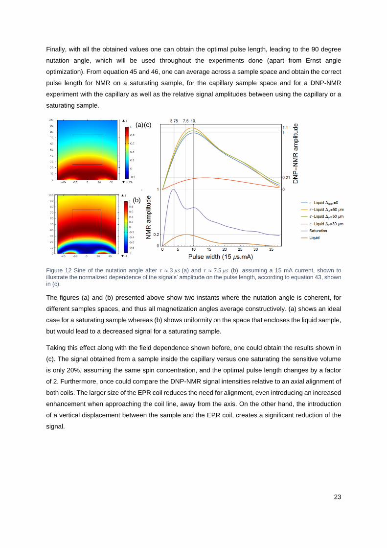
23

Finally, with all the obtained values one can obtain the optimal pulse length, leading to the 90 degree

nutation angle, which will be used throughout the experiments done (apart from Ernst angle

optimization). From equation 45 and 46, one can average across a sample space and obtain the correct

pulse length for NMR on a saturating sample, for the capillary sample space and for a DNP-NMR

experiment with the capillary as well as the relative signal amplitudes between using the capillary or a

saturating sample.

Figure 12 Sine of the nutation angle after 𝜏 ≈ 3 𝜇𝑠 (a) and 𝜏 ≈ 7.5 𝜇𝑠 (b), assuming a 15 mA current, shown to illustrate the normalized dependence of the signals’ amplitude on the pulse length, according to equation 43, shown in (c).

The figures (a) and (b) presented above show two instants where the nutation angle is coherent, for

different samples spaces, and thus all magnetization angles average constructively. (a) shows an ideal

case for a saturating sample whereas (b) shows uniformity on the space that encloses the liquid sample,

but would lead to a decreased signal for a saturating sample.

Taking this effect along with the field dependence shown before, one could obtain the results shown in

(c). The signal obtained from a sample inside the capillary versus one saturating the sensitive volume

is only 20%, assuming the same spin concentration, and the optimal pulse length changes by a factor

of 2. Furthermore, once could compare the DNP-NMR signal intensities relative to an axial alignment of

both coils. The larger size of the EPR coil reduces the need for alignment, even introducing an increased

enhancement when approaching the coil line, away from the axis. On the other hand, the introduction

of a vertical displacement between the sample and the EPR coil, creates a significant reduction of the

signal.

(a)

(b)

(c)

24

5 Mechanical holder

The project required the precise alignment of the two microchips, as the sensitive excitation height of

each coil is of the order of magnitude of its diameter (~100 µm), which in turn meant any displacement

from the ideal position would lead to a critical loss in signal/enhancement. Such a limitation is further

enhanced by the loss of field homogeneity away from the center and the necessary distance between

chips introduced by the microfluidic channel. This meant a micrometric precision would be necessary

despite most compact and commercially available setups being made in magnetic materials, mostly

steel. This created the need for the creation of a new mechanical setup.

5.1 Design

Four separate main pieces were created for design modularity and adjustability. These allowed for the

iterative adjustment of different versions of the setup as well as the fabrication of substitution pieces to

be used in the case of damage. The intricate design comes from the need of having a small holder (with

a longitudinal diameter smaller than that of the tube in which it will be inserted, 3.5 cm) with precise and

adjustable relative positions. For use in different magnet geometries, with the magnetic field direction in

either the transverse or longitudinal directions, the setup was adapted to allow for different orientations

of the microfluidics. Few mechanical constraints were implemented directly but instead as modular

pieces (as the locking structures shown below) which allowed for the reprinting of the design for other

applications, for example with materials that withstand cryogenic temperatures.

Figure 13 Full design in exploded isometric view. Dummy models for the PCB’s and microfluidics were designed to help the dimensioning. Colors shown for clarity: green for PCB’s, orange for adjustment tables and pink for microfluidics.

On Fig.14 it is shown the main holder, which will support the entire structure, and the table for the NMR

microchip. As the microfluidics will span the entire transverse length of the NMR microchip, this table

was designed to have only longitudinal adjustment due to size restrictions. Two holes for M2 screws

and another two for M1 rods are shown for fixation of the PCB to the table and for first-order alignment

with the upper system, respectively.

25

Figure 14 Isometric (a) and top (b) views of the main holder, in white, the NMR longitudinal holder, in orange, and of a model for the NMR PCB, in green. Adjusting system is also shown attached to the moving table. Motion direction indicated by arrows.

A main restriction to the setup was the impossibility of finding non-magnetic screws with sufficient

precision. This problem was avoided using a removable piece which would enclose the micrometer

screw and its thread and that could be attached to a standard M6 thread through a nut as shown above

and in detail below. This allowed for a severe reduction of the number of screws needed, as only one

adjustment is done at each moment. Movement in transverse directions, when adjusting one

microscrew, was avoided using locking pieces in that would ensure a tight fit to every guiding system,

either a rail or a pillar. A more detailed view is presented in the simulation in the next section.

The micrometric motion was achieved using a clamping piece that could rotate freely while being

longitudinally attached to the holder. This piece is then clamped to a micrometer screw, which can

precisely tune the distance in between the holder and the screw that is attached to the main holder

through its thread as seen in (b) below.

Figure 15 Microscrew cap designed, microscrew and its thread and the M6 nut used for attachment to the system (a). Only a cross section of the piece is shown for simplicity. Example of piece in application, controlling the distance from the orange wall to the black rotating piece (b). Detail of a pillar for a sliding part with the locking structures highlighted (c). Motion direction indicated by arrows.

When in the correct alignment position, the pieces would have their position locked through a small M1.6

screw connected to a nut, which would be glued to small holes designed for the effect.

On the following view, one can see the EPR holder, with xyz motion ability, as well as its vertical insertion

on the main holder’s support front and back pillars. The adjustment system is the same, but in this case

implemented in the longitudinal and transversal orientations. All rails have two sets of screws, one to

set the friction while moving and one to lock the pieces.

(a)

(b)

(a) (c)

(b)

26

Figure 16 Isometric (a) and top (b) views of the top holder, in white, the EPR longitudinal holder, in orange, and the transverse holder in white. Adjusting system is also shown attached to the moving table. Motion direction indicated by arrows.

One specific concern when designing the support was the final deflection and subsequent angular offset

when fully assembled, as the front pillar of the top table is only for locking after positioning, not active

support .This means the top table is effectively held in place by two supports. The introduction of an

angle might significantly reduce the effective magnetic field and may be mechanically prohibitive. Using

a simplified Euler-Bernoulli model for two ideal cantilevers each supporting half of a weight of 300g,

considered to be a worst case scenario for the PCB, uniformly applied along the longitudinal direction,

the linear and angular deflection were computed as 𝑤 = 𝑃𝐿4

8𝐸𝐼⁄ and 𝜃 = 𝑃𝐿3

6𝐸𝐼⁄ . These, for a cantilever

of length (L) 0.104 m, weight per unit length (P) 14.9 N/m, area moment of inertia (I) of 2.1x10-10 m4 (for

a square 5x5 mm2 section) and Young’s modulus (E) of 1283 MPa (for the EX200 plastic) amount to

𝑤 = 0.8 𝑚𝑚 and 𝜃 = 0.59°, clearly negligible amounts.

Figure 17 Isometric (a), top (b) and back (c) views of the microfluidic holder. The two symmetrical pieces are shown connected by a locking piece that can be move along the connection. Microscrew cap and microfluidics model are shown and the holes presented allow locking of the vertical motion on the pillars through M1.6 screws.

The views on figure 17 show the piece designed to hold the microfluidics. Through a vertical insertion

on the front pillars of the main holder, with the usual micrometer adjustment, one can precisely place

the holder above the NMR microchip. The microfluidic system will be interfaced with either 0.5 or 1 mm

diameter wide holes in the holder. These match the usual sizes of plastic needles and silicon flexible

tubes used as macroscopic interfaces to the micrometer wide glass capillary. To avoid any stress being

passed to the capillary, to dampen vibrations and to compensate for any size mismatch a silicon glue

will be used to fix the microfluidic system to the holder. The use of two pieces allowed for other flexible

applications, such as using only one support for the capillary to have the opposite side free for optical

inspection or interaction with the sample (e.g. laser excitation).

(a)

(b)

(a) (b) (c)

27

5.2 Simulation

The fabrication method chosen, 3D printing, requires the continuous use of a certain material throughout

the same piece, which in the case of this model was Visijet EX200, the material hardest material

available in 3D-labs, the printing retailer. As some pieces required both mechanical deformations and

undeformed use in different areas, finite element models with test loads were made to find the adequate

dimensions. 2D FEM was made in Dlubal RFEM and 3D was made using Solidwork’s simulation tool.

All simulations assume macroscopic mechanical behavior is maintained in the microscopic scale of the

1 to 100 µm meshes used and thus solve, for an isotropic, linear and elastic medium, Hook’s equation:

𝜎 = 𝐶휀 (47)

With boundary conditions that are the motion restrictions inserted through fixed or rolling joints. The

material’s characteristic were taken from the issued data sheet and were a Young modulus of 1283

MPa, a flexural modulus of 1159 MPa and a strain at break of 6.83%.

The full setup aims at a very precise alignment in three dimensions, meaning that when one is being

adjusted, the two other must remain reliably constant. This means that motion along one axis must be

slow and controlled (apart from precise, as achieved by the micrometer screws) as well as without any

sideways motion. To achieve this, one could reduce the tolerance used, but this is limited by the

precision of the printing process, which should range from 50 to 100 µm, so an alternative locking piece

was designed to press the holder laterally and avoid side motion. The lock pieces were tested to verify

their ability of compression under a normal load and under an absolute maximum load. As they are

meant to be pushed into the holders which will slide along the rails, the normal load will be that at which

the holder starts to deform away from the lock-piece. The maximum load, when fully pressed into the

support underneath, will only happen when assembling the setup (which renders material fatigue

negligible).

Figure 18 Detail of the holder sliding on the rail and lock-piece system (a) and FEM deformation result of the normal use of the system (b). The rolling joints shown model the connection of the strained holder to the rail and lock-piece. The mesh used was constant with squares of 0.1mm in side with deformations shown in µm.

Having defined the maximum pressure as that which creates a considered acceptable deformation of

35 µm, the normal working pressure was computed to be around 100kN/m2. A longer and more robust

piece at a length of ~10mm and a smaller but more fragile one at a length of ~4mm were designed for

the highest deformation possible at a normal load and a sustainable strain at the maximum load.

(a) (b)

28

The arches were designed in a parabolic shape to avoid high local strains in the middle of the piece and

a wide distance in-between the supports of the arches was chosen to have the highest possible

deformation with a certain load. The dimensions were chosen considering printing limitations; no feature

is smaller than 200 µm and the design and results have little susceptibility to a variation of 50 µm in size,

the expected error when printing.

Figure 19 Representative images of the results found. Lines with constant deformation, in µm, under a 100kN/m2 stress for the long piece (a) and strain, in absolute value for the same stress, for the small piece (b). The mesh used was variable going from 2 µm in high strain areas to 50 µm for the long piece and half for the shorter one. Dimensions shown in mm. All other results are pictured in the appendix.

The normal deformation was found to be of ~200 µm and ~150 µm for the long and short pieces,

respectively. The normal strains were found to be of 1.2 and 3.8%. The maximum strain, when the piece

touches the support, was the same for the short piece (as the support was placed 150 µm below to allow

no further deformation) and 4.3% for the long piece.

Another limitation of the setup was the attachment of the micrometer screws to a piece that would be

axially constrained but freely rotating. The screw would have to be well fixed to the pieced but maintain

the ability to be removed after adjustment. The first option was to make a cylindrical hole where the

screw would fit and where it would be fixed through an M1.6 brass screw placed perpendicularly. This

however was found to be quite bulky and restraining as it would require the access of a screwdriver in

a direction that could not be accessible. A more appropriate solution was developed with a flexing piece

that was adjusted from 3 equally spaced directions with a simple pair of tweezers.

The piece consists on a roughly conic surface going from 3.4 to 3.6 mm of diameter (with the micrometer

screw having a 3.5 mm diameter), which when compressed with two opposing forces, like when closing

a tweezer, increases slightly in diameter.

(a)

(b)

29

This allows for the entrance of the micrometer screw into the piece which is then let go and therefore

clamps the screw. The extra features in the piece are areas to place the tweezer tip and supports so

that both areas have roughly the same deformation when an equal force is applied.

Figure 20 Representation of the piece developed. Picture (a) depicts the use on the setup, clamping micrometer screw and attached to the holder that moves along the rails, as controlled by the screw. Following pictures show the FEM meshing and constraints used (b) and a top view of the piece (c).

The modelling was done using Solidworks’ modelling tool using a variable triangular mesh around

200µm in size. The fixed joints are used for software necessity, and even though they do not represent

the real constraint, no effect came from their use. The force applied was 10N on each side to represent

the maximum possible force applicable.

Figure 21 Deformation (a) and strain (b) results found under stress. Both pictures show the deformed piece, with a deformation not to scale, and the respective color code and legends.

As seen above, the maximum force applied also matches the order of magnitude of the maximum strains

advisable for the strain at break of 6.83% of the material. The deformation plot shown, indicates a radial

deformation of 20 to 30 µm, which for a radius going linearly from 1.7 to 1.8 mm, corresponds to a 20-

30% of the height of the clamping piece. For the 3mm high piece this corresponds to 0.6-0.9 mm. As

the micrometer screw used has a pitch of 0.254 mm (100 TPI), this deformation is enough to securely

clamp 2-3 threads. Any lower deformation that can clamp one entire thread should be enough for

working conditions.

(a) (b) (c)

(a) (b)

30

5.3 Fabrication

The selected method of fabrication was 3D printing due to its comparable advantages relatively to in-

house workshop work. It allowed for a much quicker fabrication with non-magnetic materials and an

easy selection of commercially available materials at a low cost. This made several setup iterations

economically viable, and allowed for the creation of a setup that can easily be reproducible and adapted

to future needs regarding two xyz tables in a confined environment.

5.3.1 Calibration/Production

3D printing, despite its astonishing developments, shows severe dependence of the build quality on the

calibration of the printer and the orientation and design of the pieces printed. Due to the need of tight

tolerances in-between moving parts, the use of highly size dependent features and of a need for

reproducibility, a set of calibration pieces was developed to study the printing limitations. The pieces

contain features in every direction and have written on them the critical dimensions.

Figure 5.22 Selected calibration pieces 3D printed for testing. The complimentary male/female pieces of the rectangular (b) and cylindrical (c) pieces are not shown. Values adapted for STL printer.

Table 3 Printing limitations obtained from the developed calibration pieces in the in-house STL printer.

These critical restrictions led to the final prototype being developed through Additively, a 3D-printing

retailer, whose database allowed for the following data, with material jetting being chosen from a local

manufacturer, 3D-LABS, for a cost that was under 10% that of a normal workshop.

Method Minimum feature (µm) Layer thickness (µm) Typical tolerance (±µm)

Stereolithography 100 16 150

Binder Jetting 100 90 130

Electron beam melting 100 50 200*

Fused deposition modeling 178 178 178*

Laser melting 40-200 30 20-50

Material jetting 100 13 25

Photopolymer jetting 150 16 25

*Can be improved through post-processing methods

Table 4 Comparison of 3D printing techniques through their mechanical accuracy and building process.

Feature Test (d in mm) Result (mm)

Min. hole

size

Long holes:0.5 to 0.9

in diameter

Vertical: 0.7,

Horizontal:0.6

Min.

feature

Sine wave with 0.05

to 2 oscillations 0.1

Tight-fit

tolerance

Male/female

connectors 3.5 to

3.825 wide

Linear: 0.094 ± 0.041

Circular: 0.22 ± 0.04

Cantilever

stiffness/

error

1.5 cm long

cantilevers: 1 to 4.5

in thickness

Usable thickness: 2.5

Edge precision: 0.2

(a)

(b)

(c)

31

5.3.2 Prototype

As observed below, the prototype was successfully implemented and after the first iterations, non-critical

pieces (seen in white) were printed in an in-house printer, due to the cost of the 3D printing. The full

setup is shown, without the PCBs, and is ready to be used and after having a sample inserted on the

capillary with a simple syringe.

Figure 23 Final prototype as implemented and used. Detail of the microfluidics (a), of the longitudinal alignment system (b) and top view of the whole setup on a piece interfacing with the bar inserted into the magnet (c).

To understand the precision ability of the system, optical-microscope images of the locking pieces (with

a hole of ~200 µm in height) and of an alignment of the capillary with the NMR coil (which is 150 µm

wide) were taken. It can be seen that alignment was visibly achieved within at least 10 µm and that the

microfluidics were constructed correctly, having the parallelepiped in the correct orientation. This can

be seen through the three distinct zones seen, in order, as wall/sample/wall (25/50/25 µm).

Figure 24 Detailed microscopic views of the long locking piece under compression until half its length (a) and under rest (b). On the right (c) a capillary is shown aligned with the center or the coil. Pictures were color corrected, for clarity, due to the much lower resolution of the camera compared to visual inspection.

300 µm

600 µm

150 µm

(a) (b)

(c)

(a) (b) (c)

32

6 Electrical interfaces

Nuclear magnetic resonance excitation was achieved using a previously fabricated microchip42 which

was wire-bonded to specially designed PCB pads, using aluminum wedge-wedge bonding, and

mechanically protected using a layer of GLOB TOP epoxy as seen on figure 24. This was done adjusting

a formerly used footprint to remove testing pads and optimizing the placement of the others to make

sure they were as parallel as possible to avoid short circuits between wires, a limitation of the technique

where wedges are created past the bonding pad. Similarly, the EPR system was implemented using a

previously made microchip, which despite unpublished is based on previous designs72 but had to be

gold bonded, using the ball-wedge technique, due to size restrictions. This was possible as the chip

carried heavy ESD protection shielding it from the voltage arc created during ball bonding.

The implementation of the PCB design was made using Altium Designer 15, the last available version

of the software. It was used for uniformity and transferability within the research group. Due to the height

of the electrical components to be used and the necessity of having both microchips within micrometric

proximity, the EPR one was designed to be used with a first stage containing all the more sizable

electrical components and a secondary stage, elevated but electrically connected to the first one, with

the microchip and the most crucial electrical components. Several design options were implemented

simultaneously for the two schematics shown.

Both PCB’s had DC inputs which were filtered using one decoupling inductor, to increase the impedance

to high frequencies, and a bypass capacitors to shunt the high frequency current to ground. It’s

noticeable on the following schematics that several capacitors, with different orders of magnitude in

capacitance, were used in parallel. This is due to the equivalent series inductance (ESL) of any

capacitor, whose impedance is usually only modelled by 𝑍𝐶 = (𝐽𝜔𝐶)−1. One can thus consider the

capacitor as a series LC system with a 1/ √𝐿𝐶 self-resonating frequency (SRF), after which the

impedance starts to grow as approximately 𝑖𝜔𝐿.

Figure 25 Evolution of the self-resonating frequency with capacitance for several KEMET RF/microwave oriented capacitors, for different packages (a). Values taken from the CDR generic official datasheet, on the left. Characteristic impedance of Texas Instruments capacitors and their advised use in parallel as stated on the RF operation guideline manual (b).

This was avoided through the use of several large capacitors with different capacitances and

consequently different SRF, with the biggest capacitor shunting more effectively at low frequencies and

the smallest capacitor at higher frequencies, where the biggest one would already be past its SRF.

(a) (b)

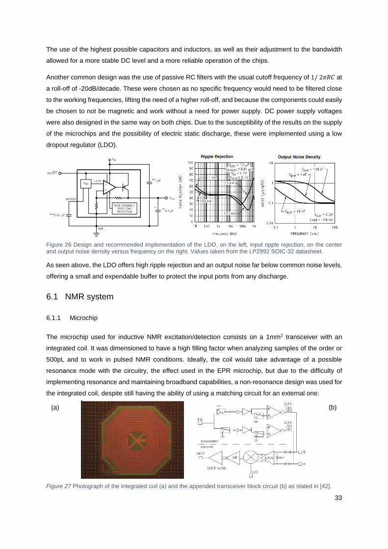
33

The use of the highest possible capacitors and inductors, as well as their adjustment to the bandwidth

allowed for a more stable DC level and a more reliable operation of the chips.

Another common design was the use of passive RC filters with the usual cutoff frequency of 1/ 2𝜋𝑅𝐶 at

a roll-off of -20dB/decade. These were chosen as no specific frequency would need to be filtered close

to the working frequencies, lifting the need of a higher roll-off, and because the components could easily

be chosen to not be magnetic and work without a need for power supply. DC power supply voltages

were also designed in the same way on both chips. Due to the susceptibility of the results on the supply

of the microchips and the possibility of electric static discharge, these were implemented using a low

dropout regulator (LDO).

Figure 26 Design and recommended implementation of the LDO, on the left, input ripple rejection, on the center and output noise density versus frequency on the right. Values taken from the LP2992 SOIC-32 datasheet.

As seen above, the LDO offers high ripple rejection and an output noise far below common noise levels,

offering a small and expendable buffer to protect the input ports from any discharge.

6.1 NMR system

6.1.1 Microchip

The microchip used for inductive NMR excitation/detection consists on a 1mm2 transceiver with an

integrated coil. It was dimensioned to have a high filling factor when analyzing samples of the order or

500pL and to work in pulsed NMR conditions. Ideally, the coil would take advantage of a possible

resonance mode with the circuitry, the effect used in the EPR microchip, but due to the difficulty of

implementing resonance and maintaining broadband capabilities, a non-resonance design was used for

the integrated coil, despite still having the ability of using a matching circuit for an external one:

Figure 27 Photograph of the integrated coil (a) and the appended transceiver block circuit (b) as stated in [42].

(a) (b)

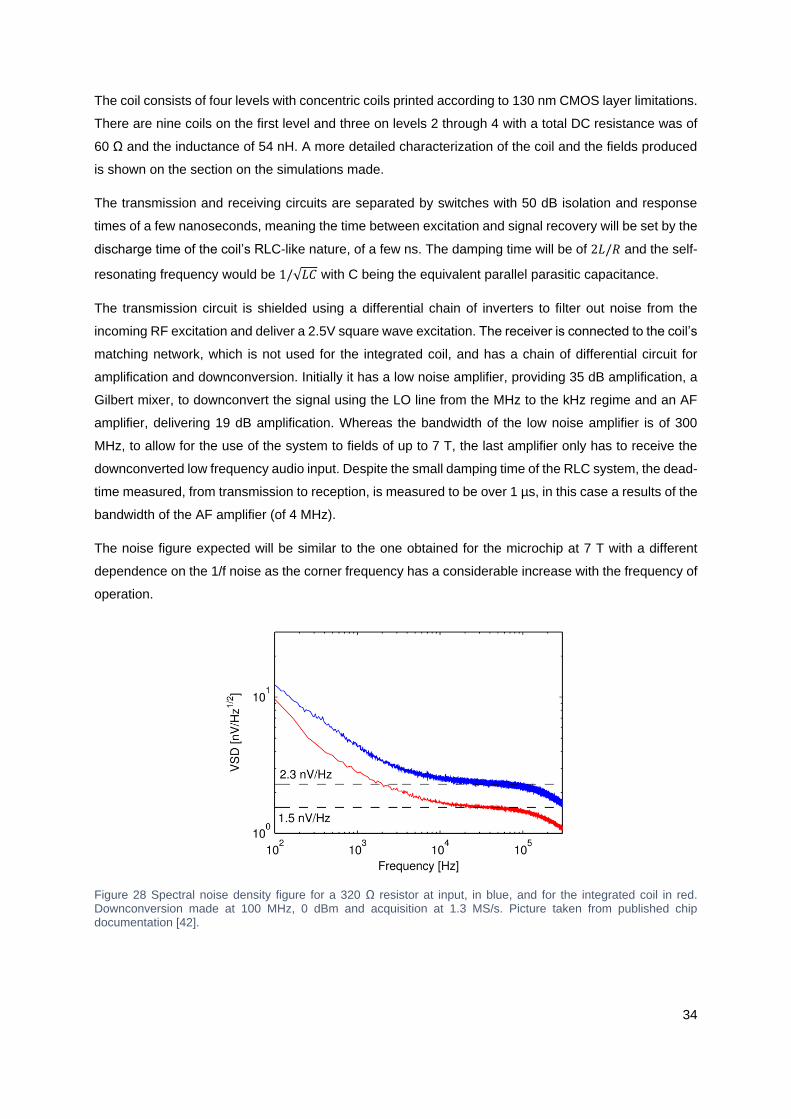
34

The coil consists of four levels with concentric coils printed according to 130 nm CMOS layer limitations.

There are nine coils on the first level and three on levels 2 through 4 with a total DC resistance was of

60 Ω and the inductance of 54 nH. A more detailed characterization of the coil and the fields produced

is shown on the section on the simulations made.

The transmission and receiving circuits are separated by switches with 50 dB isolation and response

times of a few nanoseconds, meaning the time between excitation and signal recovery will be set by the

discharge time of the coil’s RLC-like nature, of a few ns. The damping time will be of 2𝐿/𝑅 and the self-

resonating frequency would be 1/√𝐿𝐶 with C being the equivalent parallel parasitic capacitance.

The transmission circuit is shielded using a differential chain of inverters to filter out noise from the

incoming RF excitation and deliver a 2.5V square wave excitation. The receiver is connected to the coil’s

matching network, which is not used for the integrated coil, and has a chain of differential circuit for

amplification and downconversion. Initially it has a low noise amplifier, providing 35 dB amplification, a

Gilbert mixer, to downconvert the signal using the LO line from the MHz to the kHz regime and an AF

amplifier, delivering 19 dB amplification. Whereas the bandwidth of the low noise amplifier is of 300

MHz, to allow for the use of the system to fields of up to 7 T, the last amplifier only has to receive the

downconverted low frequency audio input. Despite the small damping time of the RLC system, the dead-

time measured, from transmission to reception, is measured to be over 1 µs, in this case a results of the

bandwidth of the AF amplifier (of 4 MHz).

The noise figure expected will be similar to the one obtained for the microchip at 7 T with a different

dependence on the 1/f noise as the corner frequency has a considerable increase with the frequency of

operation.

Figure 28 Spectral noise density figure for a 320 Ω resistor at input, in blue, and for the integrated coil in red. Downconversion made at 100 MHz, 0 dBm and acquisition at 1.3 MS/s. Picture taken from published chip documentation [42].

35

6.1.2 Printed circuit board

As the NMR microchip was much more critical for optimal operation of the setup its PCB was also more

complex and carefully designed, using protected I/O interfaces and low-noise components. The power

management, as well as the toggling pulse signal were introduced through unshielded but small copper

wires. The DC to DC conversion was made as usual but with the biggest capacitors fitting the board,

1206-sized 100 µF multi-layer ceramic capacitors (MLCC). The control pulse was set with the rest state

of 0V setting the chip in transmission mode contrary to normal control logic. To change this, an inverter

was set up thus changing the default state and guaranteeing a noise-reduced line. These are shown

below.

Figure 29 Schematic of the implementation of DC and digital signals on the NMR printed circuit board.

Secondly, to feed the two inverter chains which induce the square wave for coil excitation (RF) and

signal downconversion (LO), the toggle signals oscillating with a DC bias were implemented as follows.

The signal input was made using a U.FL connector, the smallest RF connector on the market, at mm

wide dimensions and working up to 6 GHz. This presented a compact solution to a noise problem

introduced on previous versions as it connected directly to a shielded SMA cable. Despite only inducing

a toggle of the inverters which create a single noiseless wave, any noise on the line will introduce a

frequency change of the toggling, similar to clock jitter, thus changing the frequency at which the signal

is downconverted and broadening the lines observed.

Figure 30 Schematic of the AC input stage of the NMR printed circuit board (a). Blocks represent the Hirose U.FL-R-SMT-1 connectors shown in (b) with its R-134G7210100CD connection cable.

The signal was then protected from ESD using two back-to-back diodes, the AT HSMS-286C-TR1G.

This solution was weighed against others (e.g. reverse polarized Zener diodes to ground and VCC) but

was chosen as it was fully functioning as a clamping device at the forward voltage of the RF diodes of

1V, even when no VCC was present. This solution was designed bearing in mind the human body model

(HBM), which models ESD spikes as current discharges in the MHz range and thousands of volts.

(a) (b)

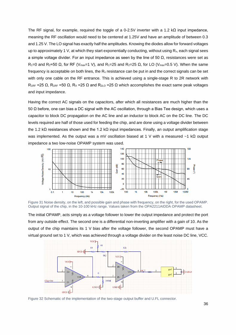
36

The RF signal, for example, required the toggle of a 0-2.5V inverter with a 1.2 kΩ input impedance,

meaning the RF oscillation would need to be centered at 1.25V and have an amplitude of between 0.3

and 1.25 V. The LO signal has exactly half the amplitudes. Knowing the diodes allow for forward voltages

up to approximately 1 V, at which they start exponentially conducting, without using Rx, each signal sees

a simple voltage divider. For an input impedance as seen by the line of 50 Ω, resistances were set as

R1=0 and R2=50 Ω, for RF (Vmax=1 V), and R1=25 and R2=25 Ω, for LO (Vmax=0.5 V). When the same

frequency is acceptable on both lines, the Rx resistance can be put in and the correct signals can be set

with only one cable on the RF entrance. This is achieved using a single-stage R to 2R network with

R1RF =25 Ω, R1RF =50 Ω, RX =25 Ω and R2LO =25 Ω which accomplishes the exact same peak voltages

and input impedance.

Having the correct AC signals on the capacitors, after which all resistances are much higher than the

50 Ω before, one can bias a DC signal with the AC oscillation, through a Bias Tee design, which uses a

capacitor to block DC propagation on the AC line and an inductor to block AC on the DC line. The DC

levels required are half of those used for feeding the chip, and are done using a voltage divider between

the 1.2 kΩ resistances shown and the 1.2 kΩ input impedances. Finally, an output amplification stage

was implemented. As the output was a mV oscillation biased at 1 V with a measured ~1 kΩ output

impedance a two low-noise OPAMP system was used.

Figure 31 Noise density, on the left, and possible gain and phase with frequency, on the right, for the used OPAMP. Output signal of the chip, in the 10-100 kHz range. Values taken from the OPA2211AIDDA OPAMP datasheet.

The initial OPAMP, acts simply as a voltage follower to lower the output impedance and protect the port

from any outside effect. The second one is a differential non-inverting amplifier with a gain of 10. As the

output of the chip maintains its 1 V bias after the voltage follower, the second OPAMP must have a

virtual ground set to 1 V, which was achieved through a voltage divider on the least noise DC line, VCC.

Figure 32 Schematic of the implementation of the two-stage output buffer and U.FL connector.

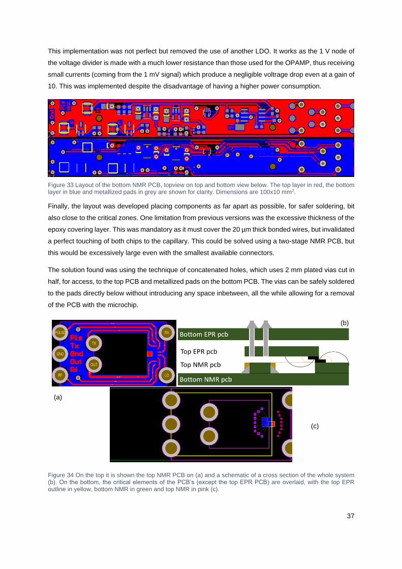
37

This implementation was not perfect but removed the use of another LDO. It works as the 1 V node of

the voltage divider is made with a much lower resistance than those used for the OPAMP, thus receiving

small currents (coming from the 1 mV signal) which produce a negligible voltrage drop even at a gain of

10. This was implemented despite the disadvantage of having a higher power consumption.

Figure 33 Layout of the bottom NMR PCB, topview on top and bottom view below. The top layer in red, the bottom layer in blue and metallized pads in grey are shown for clarity. Dimensions are 100x10 mm2.

Finally, the layout was developed placing components as far apart as possible, for safer soldering, bit

also close to the critical zones. One limitation from previous versions was the excessive thickness of the

epoxy covering layer. This was mandatory as it must cover the 20 µm thick bonded wires, but invalidated

a perfect touching of both chips to the capillary. This could be solved using a two-stage NMR PCB, but

this would be excessively large even with the smallest available connectors.

The solution found was using the technique of concatenated holes, which uses 2 mm plated vias cut in

half, for access, to the top PCB and metallized pads on the bottom PCB. The vias can be safely soldered

to the pads directly below without introducing any space inbetween, all the while allowing for a removal

of the PCB with the microchip.

Figure 34 On the top it is shown the top NMR PCB on (a) and a schematic of a cross section of the whole system (b). On the bottom, the critical elements of the PCB’s (except the top EPR PCB) are overlaid, with the top EPR outline in yellow, bottom NMR in green and top NMR in pink (c).

(a)

(b)

(c)

38

6.2 EPR system

6.2.1 Microchip

Figure 35 Block diagram of the electronics interfacing with the coil (a) and layout of the microchip (b) showing the two modes of operation: constant frequency and voltage controlled frequency. Unpublished design similar to [72].

The integrated circuit used for inductive EPR was the one shown above in both its constant and variable

frequency configuration, as based on published designs72. Due to the losses through parasitic

capacitances that entail carrying a ~20 GHz signal, it had to be implemented as two independent

oscillators (in this case a pair for the fixed oscillator and a pair for the VCO). Through the mixing of the

two signals of the pair, a downconverted signal of 1 GHz is achieved which is in this case not further

downconverted by a D-latch frequency divider (unlike the published case), thus staying in the 500-1000

MHz frequency range.

The oscillation is made through a resistive LC-oscillator, operating at 𝜔 =1

√𝐿𝐶√1 − 𝑅2𝐶

𝐿⁄ , whose resistive

dampening is compensated by a negative admittance, here implemented as a cross-coupled MOSFET

pair73. The coupling to the electron system is measured from a change in impedance, shown to be

modelled as inductive coupling to an equivalent series RLC system made by the electrons with:

𝛾𝑒𝐵0 = (𝐿𝐶)−0.5 , 𝑇2 = 2𝐿/𝑅 , 𝜂𝜒0 = 𝐿122 (48)

This frequency encoded signal is thus highly 1/f noise independent (past the transistors’ internal noise

with corner frequencies up to 1 MHz) and only affected by thermal noise, which was minimized on its

initially envisaged application of cryogenic temperature EPR. The signal is FM-demodulated through an

exterior PLL/DLL which immediately feeds the acquisition board.

Each of the coils has a 30 µm thickness and a diameter of 160 µm but due to their close proximity, these

cannot be used in near frequencies, when controlling the VCO, or for very broad peaks. This is due to

their coupled behavior when oscillating in two close frequencies, and because as a magnetic field is

swept, the resonant frequency will match both coils one after the other. As each coil may be in a different

condition, with more or less sample on top for example, the approximately symmetric signals will be

overlapped and thus not quantifiable.

(b) (a)

39

6.2.2 Printed circuit board

The PCB required different input/output signals to the EPR microchip, both DC and high frequency. The

simplest inputs were the DC ones: the bias voltages of both oscillators (OSC1,OSC2 and Ibias), of the

VCO’s (VCO1 and VCO2) and the feed voltage of the PCB, +5V.

The output signal of the chip, frequency modulated, will be of approximately 600 MHz. With the previous

considerations in mind, the EPR PCB was designed as follows.

Figure 36 Electrical schematic for the main PCB interfacing with the EPR microchip on the raised-level PCB.

The design above employs the DC filtering techniques and DC to DC conversion through the LDO, as

discussed above. As the chip outputs two phase-opposite signals, these were subtracted through an

OPAMP in a differential configuration and with a 2.5 V virtual ground. As little current is drawn, the

ground was biased using a voltage divider from the VCC voltage of 5 V.

To avoid oscillation of the OPAMP, something state on the datasheet, a 270 Ω resistor was used on the

feedback loop which in addition to the desired unitary gain (set this low as the signal is frequency

modulated) set the rest of the resistors. The OPAMP chosen was the Texas Instruments THS4304, as

it functions under high magnetic fields and low temperatures, in case the probe is used for cryogenic

measurements.

Figure 37 OPAMP’s frequency response of the noise and gain reliability, as taken from the technical datasheet.

40

Finally, knowing the bandwidth of the signal, a passive RC bandpass filter was applied between roughly

100 MHz and 1 GHz. One can also see the 0 Ω resistors to be used when the lower PCB is interfacing

with a microchip in VCO configuration. This avoids the introduction of noise when using the fixed

frequency configuration.

Figure 38 Electrical schematic for the raised-level PCB with the EPR microchip in VCO configuration (a) and fixed frequency configuration (b).

These last schematics show the simple raised level PCB’s with the most critical bypass capacitors, the

ones controlling directly the oscillator’s bias voltages, which were implemented as shown below:

Figure 39 Layout of the top PCB for use in VCO configuration, fixed frequency is omitted as it is similar. It is shown the top view’s schematic (a) and manufactured PCB in top view (b) and bottom view (c). GND pad for chip placement is highlighted. Dimensions are 20x10 mm2.

All the DC inputs shown below allowed for a use of a single cable BUS which connected, through an

intermediate connection, to another BUS. This allowed for an easily storable probe without much cabling

and a quick error-free connection.

Figure 40 Layout of the bottom PCB showing the top view (a), the bottom view (b) and the built and assembled version in top view (c). The top layer in red, the bottom layer in blue and metallized pads in grey are shown for clarity. Dimensions are 100x10 mm2.

(a) (b)

(a) (c) (b)

(a)

(b)

(c)

41

7 Results and discussion

The use of the mentioned apparatus required still several logistic adjustments and instrumentation as

well as calibration curves, all shown on the following section. The complete setup was separated in the

two different experiments possible, NMR and EPR spectrometry instrumentation, along with an NMR

Teslameter to measure the magnetic field as close to the sample as possible and an acquisition board

connected to a computer with a LabVIEW VI user interface. These were connected directly to the

compact prototype designed and inserted into the magnet through an aluminum bar.

Figure 41 Final implementations of the electrical parts as assembled on the main setup. NMR PCB in top view (a), EPR PCB in side view (b) and full design being introduced into the magnet (c). In the latter picture, the modulation coils as well as the Teslameter probe are visible inside the bore of the magnet.

7.1 Nuclear magnetic resonance

Figure 42 Block diagram of the instrumentation required for an NMR experiment. Yellow boxes show optional components. Other colors shown for simplicity.

The NMR instrumentation uses a single DC supply to power the chip and PCB at 5V, an RF source for

both the pulse excitation of the spins and the down-conversion frequency, which is inputted into the

mixer, and one amplifier. The power splitter shown allows for the use of only one source as both RF

inputs have the same frequency with one being attenuated by -3dB.

(a)

(b)

(c)

42

The time dependent free induction decay of the chip is fed through a shielded BNC cable to an amplifier

which allows for amplifications up to x5000 or a 7V saturated output. This was used to minimize the

effect of any noise coming after the amplifier and to raise the signal to voltages far above the quantization

noise of the acquisition board, therefore allowing almost any signal to be found regardless of how small

it might be compared to noise, provided enough integration time. The same amplifier allows also the

use of passive high and low-pass filters at 3, 10, 30 and 100 kHz. As the noise figure for the chip clearly

shows the 1/f noise dependence up until the thermal noise floor at 20-50 kHz, a high-pass filter is needed

to filter the highest amplitudes, including the usual 50 Hz noise, so as not to saturate the amplifier and

therefore allow a higher gain. On the other hand, the acquisition board is limited to an acquisition at

350kS/s, meaning that according to the according to the Nyquist-Shannon theorem, the highest possible

acquisition should be at 175 kHz. However, a significant noise figure at higher frequencies can be

aliased over the signal frequency, meaning they must be low-pass filtered.

To guarantee the correct function of the system, a test run with a sample saturating the sensitive volume

of the coil and with a high spin density was performed. This allowed for the best signal achievable with

the coil in an easy assembly with a piece of polydimethylsiloxane, PDMS, directly on top of the chip. For

comparison, a similar study was made using and testing a capillary filled with water. Initial studies show

the acquired data with little processing to allow for a better understanding of the instrumentation.

Figure 43 Results for a different exponential matched filters on a PDMS signal (a) of a saturating ‘infinite’ sample, at 1T, and for a distilled water sample in the studied capillary in the same conditions (b). Experimental settings described on the figures. 90º pulses and full relaxation were used (0.5 and 2s respectively).

Seeing as an FID signal decays exponentially with a characteristic time 𝑇2∗, clearly coming from field

inhomogeneity in the magnet used, the correspondent linewidth will be 1/𝑇2∗ and assuming no filtering

is added one may deduce the value from the DFT obtained. As a second step an exponential filter was

added to match the decay of the noise to that of the signal. This avoids degradation of the SNR in the

time period when the signal has decayed far beyond the noise and any further measurements would

only sample noise. However, a matched filter with a characteristic decay time of 𝑇2∗, despite presenting

the best SNR, introduces digital line broadening which may not be desirable. The spectral resolution ∆f,

dependence of the SNR and linewidth FWHM on the filtering time TFILTER are the following74.

(a) (b)

43

𝑆𝑁𝑅 ∝

(1−𝑒−𝑡 (

1

𝑇2∗ +

1𝑇𝐹𝐼𝐿𝐸𝑅

))

√𝑇𝐹𝐼𝐿𝑇𝐸𝑅 (1 − 𝑒

−2𝑡𝑇𝐹𝐼𝐿𝑇𝐸𝑅)(

1

𝑇2∗ +

1

𝑇𝐹𝐼𝐿𝑇𝐸𝑅)

, 𝐹𝑊𝐻𝑀 =1

𝜋(

1

𝑇2∗ +

1

𝑇𝐹𝐼𝐿𝑇𝐸𝑅), ∆𝑓 =

2 𝑓𝑚𝑎𝑥

𝑆𝑟𝑎𝑡𝑒 𝑇𝑎𝑐𝑞 𝐻𝑧/𝑝𝑜𝑖𝑛𝑡 (49)

Therefore, to reduce the broadening introduced by the filter, twice the original linewidth, one may use a

decay time of 𝑇2∗/2 thus reducing broadening by half and maintaining a 94% sensitivity. This will define

the spectral resolution of the measurement which must be sufficient to accurately measure the center

of a line, something achieved using at least 3 points within the line (3∆𝑓 ≤ FWHM). A smoother curve

can be achieved using zero-filling of the sample set, despite it not introducing any new information.

Inhomogeneity within the sample can be estimated through the difference between T2∗ and T2, as given

by equation (25). The T2∗ decay time of water was fitted from the peak through a Lorentzian shape and

computed as being of approximately 13 ms (75 Hz). On the other hand, the long T2 of distilled water,

characteristic of liquids, is of 2.83 s75 , meaning the sample experiences an inhomogeneous broadening

of approximately 75 Hz as well, and thus a field inhomogeneity of 1.8 µT. Due to the difficulty of

measuring the field, it is hard to establish that each peak corresponds to the correct chemical shift for

each species with absolute precision (a reference would be needed), but as component identification is

not the objective of this work, one can simply observe that the results are coherent with precession

frequencies of 42.482 and 42.466 MHz. As the current used was the same, this shift gives a rough

estimate of the reproducibility of reinserting the setup inside the magnet which, due to its hysteresis and

inhomogeneity, can induce shifts of a few kHz/mT.

To study the dependence of the SNR on the excitation/downconversion frequency and the limitation of

the available filtering frequencies of the amplifier, several runs of a PDMS sample were made in series.

This allowed for the repetition of the signal, in similar conditions, and therefore the troubleshooting of

the whole system in a methodic way. The following dependence on the output frequency was observed,

showing an improvement for frequencies away from the 1/f noise and from the cutoff frequencies of the

filters used 3, 30 and 100 KHz.

Figure 44 Dependence of the SNR on the output frequency with variable filtering conditions. Comparison made in the same experimental conditions and optimized filtering conditions. Noise figure present as background for all experiments at 1 T, for which the operating frequency and corner frequency are constant. Available corner frequencies and off-resonant excitation dependence shown for clarity.

44

As a final step of experimental calibration, and to experimentally test the simulations performed, the

dependence of the signal’s amplitude on the length of the initial pulse was studied. Using a similar probe

but with the exact same IC, adapted to a 7 T magnet used for quicker results, the same PDMS saturating

sample spectrum was studied, in the same experimental conditions, whilst changing the initial pulse

length. As the pulse’s effect is approximately independent on the stationary magnetic field and on the

sample (not sample position), the current passing through the coil, estimated to be around 20 mA, could

be derived.

Figure 45 Comparison of the results obtained experimentally, through simulation and theoretically, for a single spin, for variable pulse lengths. Experimental points taken at 7T width a 6.2 kHz off-resonance excitation and downconversion. Points were averaged 200 times with a 4 s repetition time and a 3 ms exponential filter.

The results seem to be fitting the overall dependences expected with the simulation and experimental

lines matching qualitatively, within the noise. However, the sample used was slightly different from the

modelled one, as PDSM can have variable length polymer chains, meaning a non-uniform spin

concentration, and the sample was later found to contain small air bubbles. This meant that for overall

features, such as the initial peek, when all spins are coherent, the simulation is not susceptible to point

defects and therefore accurate, but for constructive/destructive inferences the features are shown in a

less pronounced way. Having obtained the initial peak’s intensity, one can see it matches a sinusoidal

dependence, as expected from the nutation angle on a single spin, and thus from the 3.75 µs peak pulse

length, corresponding to 90º flip angle, one can compute any desired pulse sequence.

Finally, fast acquisition times will depend on the ratio 𝑇2 /𝑇1 , and for small ratios, a long time must pass

between acquisition periods. To avoid this, instead of using 90º pulses one may use a pulse inducing

the optimized Ernst76 angle of:

𝜃 = 𝑎𝑟𝑐𝑐𝑜𝑠 (𝑒−

𝑡𝐹𝐼𝐷+𝑡𝑒𝑥𝑝

𝑇1 ) (50)

Where texp refers to the experimental time from the stop of one excitation pulse until the beginning of

acquisition. At high ratios, Ernst optimization can lead to SNR increases of up to one order of magnitude

when compared to 90 º pulses as is the case of PDMS, which was found to have a 𝑇2∗ of <3 ms and a

𝑇1 of at least 3 s, as seen through changes with the repetition time. This leads to 𝑇2 /𝑇1 < 0.001 and

thus a maximum angle of 2.6º, for optimal SNR (with a negligible experimental dead time of 20 µs).

45

7.2 Electron paramagnetic resonance

Figure 46 Block diagram of the instrumentation required for an EPR experiment. Yellow boxes show optional components/systems. Other colors shown for simplicity.

Despite an easier interface with the PCB, inputting only DC control or feed voltages, the instrumentation

for the EPR was more complex as it required a changing FM demodulation circuit. The modulated output

of the PCB is amplified to match the minimum amplitude for the demodulation circuits, 1 to 3 V, and is

either demodulated using a Phase-Locked Loop or a Delay-Locked loop. In spite of the similar

demodulation, the PPL requires a frequency lock at approximately 10 MHz and allows for a dynamic

bandwidth of up to 100 kHz thus low-pass filtering any field modulation at a higher frequency. The DLL

on the other hand allows for higher frequency modulations but is much bulkier.

A systematic study was made for the EPR system with a 50 mM sample of 2,2,6,6-tetramethyl-1-

piperidinyloxyl, TEMPO in water, being analyzed on a capillary glued on top of the EPR chip allowing

for visual inspection of the alignment. This provided an understanding of the chip and a reference for

the EPR results when perfectly aligned, as that cannot be observed when using it at the same time as

the NMR setup.

Figure 47 Dependence of the EPR signal on the voltage applied on the modulation coil for magnetic field sweeps around a 0.7 T field. Sample of approximately 50 mM TEMPO in a 100 µm wide capillary perfectly aligned with the detection coil (a). Literature obtained results for a 50 mM concentration of TEMPO (b), as stated in [77].

(a) (b)

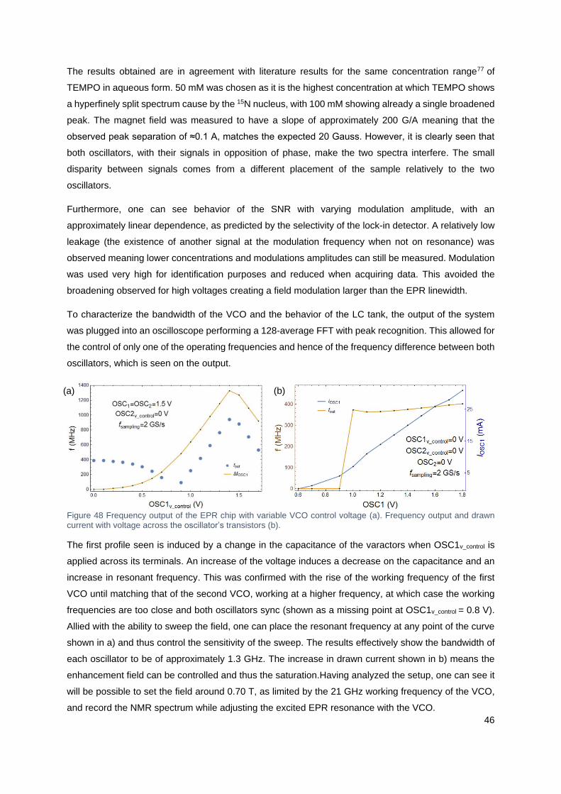
46

The results obtained are in agreement with literature results for the same concentration range77 of

TEMPO in aqueous form. 50 mM was chosen as it is the highest concentration at which TEMPO shows

a hyperfinely split spectrum cause by the 15N nucleus, with 100 mM showing already a single broadened

peak. The magnet field was measured to have a slope of approximately 200 G/A meaning that the

observed peak separation of ≈0.1 A, matches the expected 20 Gauss. However, it is clearly seen that

both oscillators, with their signals in opposition of phase, make the two spectra interfere. The small

disparity between signals comes from a different placement of the sample relatively to the two

oscillators.

Furthermore, one can see behavior of the SNR with varying modulation amplitude, with an

approximately linear dependence, as predicted by the selectivity of the lock-in detector. A relatively low

leakage (the existence of another signal at the modulation frequency when not on resonance) was

observed meaning lower concentrations and modulations amplitudes can still be measured. Modulation

was used very high for identification purposes and reduced when acquiring data. This avoided the

broadening observed for high voltages creating a field modulation larger than the EPR linewidth.

To characterize the bandwidth of the VCO and the behavior of the LC tank, the output of the system

was plugged into an oscilloscope performing a 128-average FFT with peak recognition. This allowed for

the control of only one of the operating frequencies and hence of the frequency difference between both

oscillators, which is seen on the output.

Figure 48 Frequency output of the EPR chip with variable VCO control voltage (a). Frequency output and drawn current with voltage across the oscillator’s transistors (b).

The first profile seen is induced by a change in the capacitance of the varactors when OSC1v_control is

applied across its terminals. An increase of the voltage induces a decrease on the capacitance and an

increase in resonant frequency. This was confirmed with the rise of the working frequency of the first

VCO until matching that of the second VCO, working at a higher frequency, at which case the working

frequencies are too close and both oscillators sync (shown as a missing point at OSC1v_control = 0.8 V).

Allied with the ability to sweep the field, one can place the resonant frequency at any point of the curve

shown in a) and thus control the sensitivity of the sweep. The results effectively show the bandwidth of

each oscillator to be of approximately 1.3 GHz. The increase in drawn current shown in b) means the

enhancement field can be controlled and thus the saturation.Having analyzed the setup, one can see it

will be possible to set the field around 0.70 T, as limited by the 21 GHz working frequency of the VCO,

and record the NMR spectrum while adjusting the excited EPR resonance with the VCO.

(a) (b)

47

This proved to be a simpler solution than setting the device at a fixed frequency and sweeping the field

to match the resonance, as done on the shown EPR experiment. This is simply due to the lack of

reproducibility of ferromagnets which show a significant hysteresis curve and thus make it difficult to set

the desired field after sweeping past it.

An important consideration is that of the noise on the VCO control voltages, which control the effective

oscillation frequencies. Excessive noise may deviate the oscillation from the desired frequency but a

fixed frequency will only partially excite the EPR transition. This could be solved attaching the VCO

whose field is hyperpolarizing a sample, above the NMR coil, to an AC source oscillating slightly around

the desired VCO control voltage at a higher frequency than the transverse relaxation frequency of the

electrons, seen approximately on the peak’s linewidth, however this could prove hard or impossible.

A second EPR experiment was done, on the same sample TEMPO sample, but using a VCO sweep at

a fixed field, chosen to the that of the central peak shown above in Fig 47, corresponding to a

ferromagnet current of 33.5 A. A changing VCO frequency will change proportionally the output

frequency, but as the PLL has a fixed working frequency, with saturation for frequencies outside of 9-11

MHz, one cannot simply sweep one VCO, only both. Despite using the same sweep of the control

voltage for both oscillators, the non-linear behavior of the varactors, which differ in capacitance at rest,

still leads to a varying output frequency. Nonetheless, this led the available bandwidth on a single sweep,

from saturation to saturation (0-5 V as seen below), increasing from approximately 30 to over 200 MHz.

Figure 49 EPR signal for a varying oscillation frequency at a ferromagnet current of 33.5 T, an approximately 0.7 T field. Sample of 200 mM TEMPO in a 100 µm wide capillary perfectly aligned to the detection coil.

The spectrum doesn’t matches the direct broadening of the sample studied before, at one fourth of the

concentration despite having the same central frequency (here fixed by the 33.5 T field). The width of

approximately 80 MHz, as compared to that of the three peaks shown before which span roughly 70 G

(200 MHz), is significantly sharpened through the phenomena of exchange narrowing78. As opposed to

the dipolar broadening that usually happens when the concentration is increased, the high concentration

of paramagnetic centers averages out spin interactions. This effect could be further enhanced and might

prove useful when trying to excite the entire EPR linewidth.

48

7.3 Dynamic nuclear polarization

With all setting configurations defined, one must create an alignment procedure that is reproducible and

straightforward. As both coils are not visually observable when overlapped but must be aligned within

tens of microns, a procedure based on the crosstalk between coils was used with success. Using the

same EPR instrumentation that detects a modulation of the magnetic field one can detect any other

modulation of the oscillation frequency of each oscillator. In this case it was the one induced by the

change in operating frequency caused by an induced voltage, coming from the NMR coil’s field:

Figure 50 Schematic for the alignment procedure of the NMR-DNP setup using a reproducible non-visual approach.

Observing the output of the DLL on an oscilloscope, used here to allow for a high frequency of 250 kHz,

one could identify a modulation peak easily, even when the coils were far apart, and perform a slow

adjustment until the maximum intensity of the peak. Having achieved the optimal alignment, one would

compare the results with the most similar published results shown below.

Naturally, the first step would be understanding the maximum enhancement achievable, using the

highest magnetic field possible to increase the saturation factor, as controlled by the VCO current. Given

the field is known from simulation and the enhancement is optimized, one can deduce the field and

measure the dependence of the saturation on the field generated, similarly to the results shown:

Figure 51 Saturation dependence on microwave power inside a cavity for different 14N-TEMPOL concentrations in water for a sample volume of 5 nL measured at 3.4 T (a), taken from [56]. Theoretical estimates by Armstrong and Han shown as red bars. Enhancement results for 15N-TEMPONE-D in water, for a 0.35 T field strength, irradiation time from 0.5 to 4s and 6 µL sample volume (b), taken from [79].

(a) (b)

49

A concurrent effect is that of dielectric heating of the sample as the magnetic field generating the

excitation increases. The chemical shift introduced has been found to be a good calibration of sample

temperature. The shift when irradiating can be easily measured from the TMS shift and thus calibrated.

Figure 52 Temperature induced chemical shift changes for H2O/D2O (a) and the reference TMS diluted in water (b), taken from a standardization of chemical shifts chart [80].

This has been seen to induce various effects from increased relaxation effects, line broadening and

build-up times for maximal enhancement. Similar effects to the ones presented below are expected (no

literature for TEMPO in water for the desired volume or field ranges).

Figure 53 Variation of longitudinal relaxation time, DNP build-up time and total enhancement with temperature for different concentrations of TEMPOL in ethanol. Sample in the µL range measured at 3.4 T showing the results for the CH3 (squares), CH2 (circles) and OH (triangles) peaks. Lines taken from the expected values for the given concentration as predicted by the dynamic complexation model. Image taken from [81].

The DNP-NMR results were not yet obtained, as of the writing of this document. Fabrication delays,

despite being taken into account, reduced the available experimentation time to only a few weeks at

which point the power supply of the electromagnet used stopped working thus prohibiting the acquisition

of the final enhanced results of the system. Nonetheless, the setup is fully characterized and assembled

and the results expected, within literature knowledge, are stated here.

(a) (b)

50

7.4 Conclusion and future prospects

From the obtained simulation one can see the proposed enhancement is possible but in a sub-optimal

condition. Having achieved EPR and NMR signals, it can be seen that the system is electrically ready,

characterized and optimized to perform DNP-NMR studies. Furthermore, with the accomplished cross-

talk between coils, one can be assured of the optimal achievable alignment and that there will be an

enhancement. Apart from the conclusion of the work shown, several advances can be achieved in the

future using the developed designs and simulations as they are, with slight modifications or with brand

new concepts based on the obtained results. The following suggestions are elaborated on in the

bibliography stated for the state-of-the-art section, unless otherwise noted.

Most immediately, one could adjust the system developed for other DNP-NMR enhancement studies,

as those at variable temperature, sample volume, field strength, polarizing radical and active sample.

One would also introduce a low concentration TMS standard to obtain absolute chemical shifts as well

as a quantitative measurement of the effects introduced by the variations stated above. As the NMR

probe has broadband abilities, the measurement of other NMR-sensitive nuclei, until now impossible,

could be achieved with sufficient direct enhancement or even cross polarization techniques.

Furthermore, through the same way visual inspection of the sample is done, one could couple a laser

and perform triplet-state DNP, for increased enhancement, as the capillary is fully transparent.

Another note-worthy adaptation regards sample dielectric heating. Firstly, this could be avoided using

either dissipation techniques with a more heat conductive sample holder or with a pumping system to

circulate the sample and cool it down before entering the capillary, the latter easily implemented using

the syringe interface designed. On the other hand one could avoid the microwave heating of the sample

through a change in the magnetic field. As an example, using tabled values82 for the imaginary part of

the dielectric constant of water, one can see the dielectric heating, defined as:

𝑄 = 𝜔 휀′′ 𝐸2 (51)

decreases by a factor 40 when decreasing the field strength from 1 to 0.1 T, approximately. This comes

with a loss in SNR of 56 from the field decrease, but an increase of roughly 2 on DNP-enhancement,

of 𝑇0.1 𝑇

𝑇1 𝑇⁄ , from the temperature decrease and of√

𝑡2∗0.1𝑇

𝑡2∗1𝑇

⁄ from line broadening induced by temperature

gradients across the sample. This can however allow for what would otherwise be a prohibitive study

from a sample that is evaporating from high microwave power with water evaporating at 100 ºc and

methanol at 65 ºc, for example. The simulations performed can be extended to account for heat transport

across the sample being heated according to equation (51).

The natural follow-up of the obtained results is to integrate both coils in a single CMOS microchip, whose

geometry could be simulated using the developed simulation. This would allow a much easier alignment,

with only the placement of one chip and the sample holder, and a higher enhancement, as the highest

contributing spins close to NMR coil would also have the highest enhancement. On the other hand, the

integrated use of two coils that close introduces several limitations.

51

The sizes of the two coils are similar, the NMR one limited by sensitive volume and the EPR one by the

wavelength of the resonating frequency, which means they could not be coplanar and a distance would

have to be introduced between both, within the CMOS layer’s limitations. Furthermore, the close

proximity could introduce electromagnetic effects between both coils, either capacitive shunting or

induced currents, thus reducing the effective current/field or generating noise. Nonetheless, having a

fully integrated design would then open up the possibility for further coupling to other techniques. Among

these are the ones mentioned before, such as triplet-DNP, and complementary techniques such as

microfabrication of the coil or the sample holder and eventually MAS or array parallelization.

Parallelization has been achieved by the group with earlier probe versions43, in an 8-array with 500 µm

wide coils with 50 times smaller spin sensitivity, but did not include on-chip downconversion. This tightly

packed 350 nm CMOS integrated array had the problem of electrical crosstalk between coils but

achieved an advance towards massively parallel solutions for spectroscopy or imaging, possibly

incorporating DNP-NMR capabilities as well.

Post-CMOS array fabrication is also an achieved technique83 usually using a thin interface layer (e.g.

5nm of titanium) to allow the fabrication of structures. These allow for highly optimized sample holders,

with the sample even being inserted into a resonant planar coil, fabricated with a high aspect ratio84,85,

or interfaced with microfluidics structures. This would allow for the use of different coil geometries, fluid

manipulation techniques (e.g. electrophoresis) and even the placement of magnetic structures to avoid

susceptibility mismatches.

Despite the lengthy and difficult process of achieving such an array with both integrated coils and with

the structures microfabricated on top, these could achieve record high spin-sensitivities, and allow for a

cheap and compact solution easily coupled to other techniques for non-invasive sample analysis.

52

8 Bibliography

1. Bloch, F., Hansen, W. W. & Packard, M. The nuclear induction experiment. Phys. Rev. 70, 474–485 (1946). 2. Purcell, E., Torrey, H. & Pound, R. Resonance Absorption by Nuclear Magnetic Moments in a Solid. Phys.

Rev. 69, 37–38 (1946). 3. Carver, T. R. & Slichter, C. P. Experimental Verification of the Overhauser Nuclear Polarization Effect. Phys.

Rev. 102, 975–980 (1956). 4. Lauterbur, P. C. Image Formation by Induced Local Interactions: Examples Employing Nuclear Magnetic

Resonance. Nature 242, 190–191 (1973). 5. Bottomley, P. a. NMR imaging techniques and applications: a review. Rev. Sci. Instrum. 53, 1319–1337

(1982). 6. Sinanna, a. et al. Field stabilization of the Iseult/Inumac magnet operating in driven mode. IEEE Trans.

Appl. Supercond. 20, 790–793 (2010). 7. Graessl, A. et al. Modular 32-channel transceiver coil array for cardiac MRI at 7.0T. Magn. Reson. Med. 72,

276–290 (2014). 8. Bernstein, M. A., King, K. E., Zhou, X. J. & Fong, W. Handbook of MRI Pulse Sequences. Medical Physics

32, 1452 (2005). 9. Aguayo, J. B., Blackband, S. J., Schoeniger, J., Mattingly, M. A. & Hintermann, M. Nuclear magnetic

resonance imaging of a single cell. Nature 322, 190–1 (1986). 10. Ciobanu, L., Seeber, D. . & Pennington, C. . 3D MR microscopy with resolution by by. J. Magn. Reson. 158,

178–182 (2002). 11. Göbel, K. et al. Phased-array of microcoils allows MR microscopy of ex vivo human skin samples at 9.4 T.

Skin Res. Technol. 21, 61–8 (2015). 12. Nationalmaglab.org. MagLab - The largest and highest powered magnet lab in the world (2015). at

<https://nationalmaglab.org/> 13. Bird, M. D., Dixon, I. R. & Toth, J. Large, High-Field Magnet Projects at the NHMFL. IEEE Trans. Appl.

Supercond. 25, 1–6 (2015). 14. Society, A. P. American ysi. New York (1955). 15. Wu, M. K. et al. Superconductivity at 93 K in a new mixed-phase Y-Ba-Cu-O compound system at ambient

pressure. Phys. Rev. Lett. 58, 908–910 (1987). 16. J. Stepisnik, V. Erzen, M. K. NMR imaging in the Earth’s magnetic field. Magn. Reson. Imag. 15 386–391,

(1990). 17. Appelt, S. et al. NMR spectroscopy in the milli-Tesla regime: Measurement of 1H chemical-shift differences

below the line width. Chem. Phys. Lett. 485, 217–220 (2010). 18. Vanzijl, P. C. M., Sukumar, S., Johnson, M. O., Webb, P. & Hurd, R. E. Optimized Shimming for High-

Resolution NMR Using Three-Dimensional Image-Based Field Mapping. J. Magn. Reson. Ser. A 111, 203–207 (1994).

19. Schneider, E. & Glover, G. Rapidin vivo proton shimming. Magn. Reson. Med. 18, 335–347 (1991). 20. Olson, D. L., Peck, T. L., Webb, A. G., Magin, R. L. & Sweedler, J. V. High-Resolution Microcoil 1H-NMR

for Mass-Limited, Nanoliter-Volume Samples. Science (80-. ). 270, 1967–1970 (1995). 21. Fuks, L. ., Huang, F. S. ., Carter, C. ., Edelstein, W. . & Roemer, P. . Susceptibility, lineshape, and shimming

in high-resolution NMR. J. Magn. Reson. 100, 229–242 (1992).

53

22. Stejskal, E. ., Schaefer, J. & Waugh, J. . Magic-angle spinning and polarization transfer in proton-enhanced NMR. J. Magn. Reson. 28, 105–112 (1977).

23. Chmelka, B. F. et al. Oxygen-17 NMR in solids by dynamic-angle spinning and doublerotation. Nature 339,

42–43 (1989). 24. De Paëpe, G. Dipolar recoupling in magic angle spinning solid-state nuclear magnetic resonance. Annu.

Rev. Phys. Chem. 63, 661–84 (2012). 25. Samoson, A. et al. New horizons for magic-angle spinning NMR. Top. Curr. Chem. 246, 15–31 (2005). 26. Lawler, R. G. & Barbara, P. F. Practical aspects of quantitative CIDNP using FT NMR. J. Magn. Reson. 40,

135–155 (1980). 27. Hyperpolarization Methods in NMR Spectroscopy | Lars T. Kuhn | Springer. at

<https://www.springer.com/us/book/9783642397271> 28. Adams, R. W. et al. Reversible interactions with para-hydrogen enhance NMR sensitivity by polarization

transfer. Science 323, 1708–11 (2009). 29. Reese, M. et al. (1)H and (13)C dynamic nuclear polarization in aqueous solution with a two-field (0.35 T/14

T) shuttle DNP spectrometer. J. Am. Chem. Soc. 131, 15086–7 (2009). 30. Maly, T. et al. Dynamic nuclear polarization at high magnetic fields. J. Chem. Phys. 128, 052211 (2008). 31. Ardenkjaer-Larsen, J. H. et al. Increase in signal-to-noise ratio of > 10,000 times in liquid-state NMR. Proc.

Natl. Acad. Sci. U. S. A. 100, 10158–63 (2003). 32. Bornet, A., Melzi, R., Jannin, S. & Bodenhausen, G. Cross Polarization for Dissolution Dynamic Nuclear

Polarization Experiments at Readily Accessible Temperatures 1.2 < T < 4.2 K. Appl. Magn. Reson. 43, 107–117 (2012).

33. Ahuja, P., Sarkar, R., Jannin, S., Vasos, P. R. & Bodenhausen, G. Proton hyperpolarisation preserved in

long-lived states. Chem. Commun. (Camb). 46, 8192–4 (2010). 34. Stevanato, G. et al. A Nuclear Singlet Lifetime of More than One Hour in Room-Temperature Solution.

Angew. Chemie Int. Ed. 54, 3740–3743 (2015). 35. Odelblad, E. Micro-NMR in high permanent magnetic fields. (1966). 36. Olson, D. L., Lacey, M. E. & Sweedler, J. V. High-resolution microcoil NMR for analysis of mass-limited,

nanoliter samples. Anal. Chem. 70, 645–650 (1998). 37. Heselmeyer-Haddad, K. et al. Single-cell genetic analysis of ductal carcinoma in situ and invasive breast

cancer reveals enormous tumor heterogeneity yet conserved genomic imbalances and gain of MYC during progression. Am. J. Pathol. 181, 1807–22 (2012).

38. Olson, D. L., Lacey, M. E. & Sweedler, J. V. High-Resolution Microcoil NMR for Analysis of Mass-Limited,

Nanoliter Samples. Anal. Chem. 70, 645–650 (1998). 39. Lam, M. H. C., Homenuke, M. A., Michal, C. A. & Hansen, C. L. Sub-nanoliter nuclear magnetic resonance

coils fabricated with multilayer soft lithography. J. Micromechanics Microengineering 19, 095001 (2009). 40. Behnia, B. & Webb, A. G. Limited-sample NMR using solenoidal microcoils, perfluorocarbon plugs, and

capillary spinning. Anal. Chem. 70, 5326–31 (1998). 41. Wu, W. et al. The design and fabrication of a low-field NMR probe based on a multilayer planar microcoil.

Microsyst. Technol. 20, 419–425 (2013). 42. Grisi, M., Gualco, G. & Boero, G. A broadband single-chip transceiver for multi-nuclear NMR probes. Rev.

Sci. Instrum. 86, 044703 (2015). 43. Anders, J., Chiaramonte, G., SanGiorgio, P. & Boero, G. A single-chip array of NMR receivers. J. Magn.

Reson. 201, 239–249 (2009). 44. Fratila, R. M., Gomez, M. V., Sýkora, S. & Velders, A. H. Multinuclear nanoliter one-dimensional and two-

54

dimensional NMR spectroscopy with a single non-resonant microcoil. Nat. Commun. 5, 3025 (2014). 45. Mohmmadzadeh, M. et al. Characterization of a 3D MEMS fabricated micro-solenoid at 9.4 T. J. Magn.

Reson. 208, 20–6 (2011). 46. Uchiyama, S. et al. Novel MEMS-based fabrication technology of micro solenoid-type inductor. J.

Micromechanics Microengineering 23, 114009 (2013). 47. Li, Y., Wolters, A. M., Malawey, P. V., Sweedler, J. V. & Webb, A. G. Multiple Solenoidal Microcoil Probes

for High-Sensitivity, High-Throughput Nuclear Magnetic Resonance Spectroscopy. Anal. Chem. 71, 4815–4820 (1999).

48. van Bentum, P. J. M., Janssen, J. W. G., Kentgens, A. P. M., Bart, J. & Gardeniers, J. G. E. Stripline probes

for nuclear magnetic resonance. J. Magn. Reson. 189, 104–13 (2007). 49. Bart, J., Janssen, J. W. G., van Bentum, P. J. M., Kentgens, A. P. M. & Gardeniers, J. G. E. Optimization

of stripline-based microfluidic chips for high-resolution NMR. J. Magn. Reson. 201, 175–85 (2009). 50. Murashige, K. & Dohi, T. The micro saddle coil with switchable sensitivity for Magnetic Resonance Imaging.

in 2015 28th IEEE International Conference on Micro Electro Mechanical Systems (MEMS) 674–677 (IEEE, 2015). doi:10.1109/MEMSYS.2015.7051047

51. Alonso, J., Soleilhavoup, A., Wong, A., Guiga, A. & Sakellariou, D. Double helix dipole design applied to

magnetic resonance: a novel NMR coil. J. Magn. Reson. 235, 32–41 (2013). 52. Jones, C. J. & Larive, C. K. Could smaller really be better? Current and future trends in high-resolution

microcoil NMR spectroscopy. Anal. Bioanal. Chem. 402, 61–8 (2012). 53. Gfrörer, P., Schewitz, J., Pusecker, K. & Bayer, E. Peer Reviewed: On-Line Coupling of Capillary

Separation Techniques with 1H NMR. Anal. Chem. 71, 315A–21A (1999). 54. Sharma, M., Janssen, G., Leggett, J., Kentgens, A. P. M. & van Bentum, P. J. M. Rapid-melt Dynamic

Nuclear Polarization. J. Magn. Reson. 258, 40–48 (2015). 55. Villanueva-Garibay, J. A., Annino, G., van Bentum, P. J. M. & Kentgens, A. P. M. Pushing the limit of liquid-

state dynamic nuclear polarization at high field. Phys. Chem. Chem. Phys. 12, 5846–9 (2010). 56. van Bentum, P. J. M., van der Heijden, G. H. A., Villanueva-Garibay, J. A. & Kentgens, A. P. M. Quantitative

analysis of high field liquid state Dynamic Nuclear Polarization. Phys. Chem. Chem. Phys. 13, 17831–40 (2011).

57. Abragam, A. The Principles of Nuclear Magnetism. (1961). at

<https://books.google.ch/books/about/The_Principles_of_Nuclear_Magnetism.html?id=9M8U_JK7K54C&pgis=1>

58. Hore, P. J. Nuclear Magnetic Resonance. (Oxford University Press, 2015). 59. Günther, U. L. Dynamic nuclear hyperpolarization in liquids. Top. Curr. Chem. 335, 23–69 (2013). 60. Hovav, Y., Feintuch, A. & Vega, S. Dynamic nuclear polarization assisted spin diffusion for the solid effect

case. J. Chem. Phys. 134, 074509 (2011). 61. Solomon, I. Relaxation Processes in a System of Two Spins. Phys. Rev. 99, 559–565 (1955). 62. Bennati, M., Tkach, I. & Türke, M.-T. Electron Paramagnetic Resonance. 22, (Royal Society of Chemistry,

2010). 63. Lima, M. M. R. a, Monteiro, R. C. C., Graça, M. P. F. & Ferreira Da Silva, M. G. Structural, electrical and

thermal properties of borosilicate glass-alumina composites. J. Alloys Compd. 538, 66–72 (2012). 64. CRC Handbook of Chemistry and Physics, 96th Edition (CRC Handbook of Chemistry & Physics): William

M. Haynes: 9781482260960: Amazon.com: Books. at <http://www.amazon.com/Handbook-Chemistry-Physics-96th-Edition/dp/1482260964>

65. Hurd, C. M. Low temperature magnetic susceptibility of pyrex, fused quartz, and polytetrafluoroethylene.

Rev. Sci. Instrum. 37, 515–516 (1966).

55

66. Dimitrakakis, G. S. & Tatakis, E. C. High-frequency copper losses in magnetic components with layered

windings. IEEE Trans. Magn. 45, 3187–3199 (2009). 67. Rusiniak, L. Electric properties of water. New experimental data in the 5Hz-13MHz frequency range. ACTA

Geophys. Pol. 52, 63–76 (2004). 68. Schenck, J. F. The role of magnetic susceptibility in magnetic resonance imaging: MRI magnetic

compatibility of the first and second kinds. Med. Phys. 23, 815 (1996). 69. Hoult, D. . & Richards, R. . The signal-to-noise ratio of the nuclear magnetic resonance experiment. J.

Magn. Reson. 24, 71–85 (1976). 70. Hoult, D. I. The principle of reciprocity in signal strength calculations?A mathematical guide. Concepts

Magn. Reson. 12, 173–187 (2000). 71. Neugebauer, P. et al. Liquid state DNP of water at 9.2 T: an experimental access to saturation. Phys. Chem.

Chem. Phys. 15, 6049–56 (2013). 72. Gualco, G. et al. Cryogenic single-chip electron spin resonance detector. J. Magn. Reson. 247, 96–103

(2014). 73. Boero, G. et al. Room temperature strong coupling between a microwave oscillator and an ensemble of

electron spins. J. Magn. Reson. 231, 133–140 (2013). 74. Spencer, R. G. The Time-Domain Matched Filter and the Spectral-Domain Matched Filter in 1-Dimensional

NMR Spectroscopy. Concepts Magn. Reson. Part A. Bridg. Educ. Res. 36A, 255–264 (2010). 75. James, T. L. & Gillen, K. T. Nuclear magnetic resonance relaxation time and self-diffusion constant of water

in hen egg white and yolk. Biochim. Biophys. Acta - Gen. Subj. 286, 10–15 (1972). 76. Ernst, R. R. Application of Fourier Transform Spectroscopy to Magnetic Resonance. Rev. Sci. Instrum. 37,

93 (1966). 77. Ablett, S., Barratt, M. D. & Franks, F. Self-diffusion and electron spin exchange of hydrophobic probes in

dilute solution. J. Solution Chem. 4, 797–807 (1975). 78. Anderson, P. W. & Weiss, P. R. Exchange Narrowing in Paramagnetic Resonance. Rev. Mod. Phys. 25,

269–276 (1953). 79. Türke, M.-T., Tkach, I., Reese, M., Höfer, P. & Bennati, M. Optimization of dynamic nuclear polarization

experiments in aqueous solution at 15 MHz/9.7 GHz: a comparative study with DNP at 140 MHz/94 GHz. Phys. Chem. Chem. Phys. 12, 5893–901 (2010).

80. Hoffman, R. E. Standardization of chemical shifts of TMS and solvent signals in NMR solvents. Magn.

Reson. Chem. 44, 606–16 (2006). 81. van der Heijden, G. H. A., Kentgens, A. P. M. & van Bentum, P. J. M. Liquid state dynamic nuclear

polarization of ethanol at 3.4 T (95 GHz). Phys. Chem. Chem. Phys. 16, 8493–502 (2014). 82. Meissner, T. & Wentz, F. J. The complex dielectric constant of pure and sea water from microwave satellite

observations. IEEE Trans. Geosci. Remote Sens. 42, 1836–1849 (2004). 83. Mason, A., Greiner, A. J., Ofoli, R. Y. & Worden, R. M. Post-CMOS Compatible Microfabrication of a Multi-

Analyte Bioelectrochemical Sensor Array Microsystem. in 2006 5th IEEE Conference on Sensors 612–615 (IEEE, 2006). doi:10.1109/ICSENS.2007.355542

84. Kohlmeier, T., Seidemann, V., Bottgenbach, S. & Gatzen, H. H. An investigation on technologies to fabricate microcoils for miniaturized actuator systems. Microsyst. Technol. 10, 175–181 (2004).

85. Brunet, M., O'Donnell, T., O'Brien, J., McCloskey, P. & Mathuna, S. C. Mathuba. Thick photoresist

development for the fabrication of high aspect ratio magnetic coils. J. Micromechanics Microengineering 12, 444–449 (2002).

56

Appendix

i

Appendix

A. FEM simulations

The rail and lock-piece designs were computed for a rest compression of roughly 100 microns, to

overcome printing limitations in currently available machines. All the values are taken for the chosen

material, EX200, as stated on the section with the abridged graphics concerning this simulation. The

overlapping table rail will start to bend excessively and eventually break past a stress of 100 kN/m2, as

seen on the results found below.

Figure I Dlubal RFEM strain and deformation results of the system in normal use conditions. The rolling joints shown model the connection of the strained holder to the rail and lock-piece. The mesh used was constant with squares of 0.1mm in side. Deformation shown in µm, stress in kN/m2 (100.0) and strain in absolute value.

Under the landmark stress, the following results strain and deformations were found:

Figure II Dlubal RFEM strain and deformation results of the small locking piece in normal use conditions. The rolling joints shown model the connection to neighboring pieces. The mesh used was variable and adapted to high-gradient areas. Deformation shown in µm, stress in kN/m2 (100.0) and strain in absolute value.

ii

The computations made show the optimized geometry and deformations for the short piece above (used

for the transverse motion axis of the EPR table and microfluidics pillars) and the long piece below (for

other motion axes). The shape of the arch if a parabola to avoid local stresses when bending and all are

protected with a base to avoid over-compression and possible critical strains.

Figure III Dlubal RFEM strain and deformation results of the large locking piece in normal use conditions. The rolling joints shown model the connection to neighboring pieces. The mesh used was variable and adapted to high-gradient areas. Deformation shown in µm, stress in kN/m2 (100.0) and strain in absolute value.

B. Technical drawings

The following pages show the technical drawings of the pieces designed with the sufficient dimensions

to reproduce the work done. Some dimensions were omitted as they can be chosen with few limitations

and others are a consequence of the tolerance used. Printing limitations were set for the outside

diameter which could not exceed the 3.5 cm diameter of the magnet borehole that the setup must fit

and 3D printing requirements. These require feature sizes over 100-200 µm, depending on printing

orientation, tolerances of 100 µm for tight-fit sliding of pieces and adjusted screw holes for the available

PCB’s and screw dimensions.

3

149.90

14

2.40 2.40 5 5

2.40

1.5

0

3

1.80 B

B

93

15

1.

80

1.

80

5 5

M6 thread

Variable PCBattachment

Details specifiedon thesis document

4.5

0

3

6

3.1

0

SECTION B-BSCALE 1 : 1

ASSEMBLY bottom table

WEIGHT:

A4

SHEET 1 OF 1SCALE1:1

DWG NO.

TITLE:

REVISION

MATERIAL:EX200 by 3DLabs

DATESIGNATURENAME

DEBUR AND BREAK SHARP EDGES

FINISH:UNLESS OTHERWISE SPECIFIED:DIMENSIONS ARE IN MILIMETERSSURFACE FINISH: N/ATOLERANCES: LINEAR: 0.1 ANGULAR:-

Q.A

MFG

APPV'D

CHK'D

DRAWN NMR longitudinal adjustment table

6

3.60

7

7

B

B

2

1

15

17

3

AA

2.

20

5

SECTION A-A

2.4

0

2.40 SECTION B-B

ASSEMBLY microfluidic holder transverse

WEIGHT:

A4

SHEET 1 OF 1SCALE:2:1

DWG NO.

TITLE:

REVISION

MATERIAL:EX200 by 3DLABS

DATESIGNATURENAME

DEBUR AND BREAK SHARP EDGES

FINISH:UNLESS OTHERWISE SPECIFIED:DIMENSIONS ARE IN MILLIMETERSSURFACE FINISH:TOLERANCES: LINEAR: 0.1 ANGULAR:

Q.A

MFG

APPV'D

CHK'D

DRAWN Vertical adjustment microfluidics holder

5 4.80

5

13

13

5 3 3

BB

10

10

34.

22

43

27.

30

9

25

23.

90

2.20

2.20

3.6

0

3.60

6

M6 thread

Details specified on thesis document

Variable PCBattachment

M1.6 locking screws

12 5 7.90 15

1.7

8

100 5 10 2.60

17

2.60

SECTION B-BSCALE 1 : 1

ASSEMBLY top tableWEIGHT:

A4

SHEET 1 OF 1SCALE1:1

DWG NO.

TITLE:

REVISION

MATERIAL:EX200 by 3DLABS

DATESIGNATURENAME

DEBUR AND BREAK SHARP EDGES

FINISH:UNLESS OTHERWISE SPECIFIED:DIMENSIONS ARE IN MILLIMETERSSURFACE FINISH:TOLERANCES: 0.1 LINEAR: ANGULAR:

Q.A

MFG

APPV'D

CHK'D

DRAWN

EPR xyz adjustment table