WATER RESOURCES RESEARCH, VOL. ???, XXXX, DOI:10.1029/,

A Divide and Conquer Approach to Cope with1

Uncertainty, Human Health Risk and Decision2

Making in Contaminant Hydrology3

Felipe P. J. de Barros1, Diogo Bolster

2, Xavier Sanchez-Vila

3and Wolfgang

Nowak4

F.P.J. de Barros, Institute of Applied Analysis and Numerical Simulation/SimTech, Pfaffen-

waldring 57, University of Stuttgart, 70569 Stuttgart, Germany. (felipe.debarros@simtech.uni-

stuttgart.de)

1Institute of Applied Analysis and

D R A F T January 14, 2011, 2:05pm D R A F T

X - 2 DE BARROS ET AL.: DIVIDE & CONQUER: UNCERTAINTY, RISK & DECISIONS IN HYDROLOGY

Abstract. Assessing health risk in hydrological systems is an interdis-4

ciplinary field. It relies on the expertise in fields of hydrology and public health5

and needs powerful translation concepts to provide decision support and pol-6

icy making. Reliable health risk estimates need to account for the uncertain-7

ties and variabilities present in hydrological, physiological and human be-8

havioral parameters. Despite significant theoretical advancements in stochas-9

tic hydrology, there is still a dire need to further propagate these concepts10

to practical problems and to society in general. Following a recent line of work,11

Numerical Simulation/SimTech,

Pfaffenwaldring 57, University of Stuttgart,

70569 Stuttgart, Germany

2Environmental Fluid Dynamics

Laboratories, Dept. of Civil Engineering

and Geological Sciences, University of Notre

Dame, IN 46556, USA.

3Dept. of Geotechnical Engineering and

Geosciences, Technical University of

Catalonia, E-08034 Barcelona, Spain.

4Institute of Hydraulic Engineering,

LH2/SimTech, University of Stuttgart,

Pfaffenwaldring 61, 70569 Stuttgart,

Germany.

D R A F T January 14, 2011, 2:05pm D R A F T

DE BARROS ET AL.: DIVIDE & CONQUER: UNCERTAINTY, RISK & DECISIONS IN HYDROLOGY X - 3

we use of fault trees to address the task of probabilistic risk analysis (PRA)12

and to support related decision and management problems. Fault trees al-13

low to decompose the assessment of health risk into individual manageable14

modules, thus tackling a complex system by a structural divide and conquer15

approach. The complexity within inside each module can be chosen individ-16

ually according to data availability, parsimony, relative importance and stage17

of analysis. Three differences are highlighted in the current paper when com-18

pared to previous works: (1) The fault tree proposed here accounts for the19

uncertainty in both hydrological and health components, (2) system failure20

within the fault tree is defined in terms of risk being above a threshold value21

whereas previous studies that used fault trees used auxiliary events such as22

exceedance of critical concentration levels and (3) we introduce a new form23

of stochastic fault tree that allows to weaken the assumption of independent24

subsystems that is required by a classical fault tree approach. We illustrate25

our concept in a simple groundwater-related setting.26

D R A F T January 14, 2011, 2:05pm D R A F T

X - 4 DE BARROS ET AL.: DIVIDE & CONQUER: UNCERTAINTY, RISK & DECISIONS IN HYDROLOGY

1. Introduction

Assessing the impact of water pollutants on human health relies on our ability to accu-27

rately assess two things: first, the transport and possible reactions between contaminants28

in a hydrosystem and second, evaluating the physiological response of humans to such29

contaminants and the resulting adverse effects on human health [e.g., Andricevic and30

Cvetkovic, 1996; Maxwell et al., 1998; Maxwell and Kastenberg , 1999; Maxwell et al.,31

1999; Benekos et al., 2007; de Barros and Rubin, 2008; Maxwell et al., 2008]. Notori-32

ously, both of these fields contain uncertainty for a variety of reasons. These include33

the lack of characterization data, inadequate conceptual models and the occurrence of34

natural variability in both hydrosystems and health components [Bogen and Spear , 1987;35

McKone and Bogen, 1991; Burmaster and Wilson, 1996; Maxwell and Kastenberg , 1999].36

Given such uncertainties, following the traditional route of making single deterministic37

predictions for a given scenario has little practical purpose [USEPA, 2001]. This fact has38

been recognized in recent times by many large-scale government regulatory bodies. As a39

consequence, they increasingly insist on the use of probabilistic approaches that include40

estimates in uncertainty of risk [e.g., Rubin et al., 1994; Andricevic and Cvetkovic, 1996;41

Davison et al., 2005; Persson and Destouni , 2009].42

In an ideal world with extensive computational resources, one might try to tackle43

such water-related health impact problems in a probabilistic framework by running high-44

resolution Monte-Carlo simulations of the entire interacting system at full complexity.45

However, the multi-component (and multi-scale) nature of these problems can often ren-46

der such an approach difficult (if not impossible) to implement in practice. On the hy-47

D R A F T January 14, 2011, 2:05pm D R A F T

DE BARROS ET AL.: DIVIDE & CONQUER: UNCERTAINTY, RISK & DECISIONS IN HYDROLOGY X - 5

drological side of the problem, heterogeneity in many physical and chemical parameters48

can range over multiple orders of magnitude and lead to scale-dependence of process de-49

scriptions. Depending on the specific problem at hand and the contaminants in question,50

the number of required parameters can be very large, far beyond parsimony, with lim-51

ited spatial resolution of the hydrosystem [Rubin, 2003; Tartakovsky and Winter , 2008].52

Similarly, on the health side, natural variability in human behavior, age, body type and53

genetic characteristics (to mention but a few) lead to large variability in physiological54

parameters [e.g., Maxwell and Kastenberg , 1999].55

Apart from the unresolved issues with natural variability that occur in both parts of56

the system, it is not even entirely clear that the conceptual mathematical models used in57

each field are fully appropriate. For example, in hydrogeology, there is an ever increasing58

number of field, laboratory and numerical data sets, indicating that “anomalous”behavior59

(i.e. non-Fickian phenomena that cannot be described by the traditional advection dis-60

persion equation approaches) may in fact not be all that anomalous but rather the rule61

[e.g., Gelhar et al., 1992; Sidle et al., 1998; Silliman et al., 1997; Levy and Berkowitz ,62

2003; Fiori et al., 2007]. Such anomalies, observed in conservative transport, pose even63

further complications for the transport of reactive solutes [Raje and Kapoor , 2000; Gram-64

ling et al., 2002]. However, there is a continuous emergence of new models that appear65

capable of capturing these effects [e.g., Neuman and Tartakovsky , 2009; Benson and Meer-66

schaert , 2008; Donado et al., 2009; Bolster et al., 2010; Edery et al., 2009]. On the health67

side, many of the mathematical dose-response models rely on linear extrapolation of data68

from high-dose laboratory experiments on animals [Fjeld et al., 2007], which do not take69

into account the possibility of nonlinear behavior at lower doses [Bogen and Spear , 1987;70

D R A F T January 14, 2011, 2:05pm D R A F T

X - 6 DE BARROS ET AL.: DIVIDE & CONQUER: UNCERTAINTY, RISK & DECISIONS IN HYDROLOGY

McKone and Bogen, 1991; Burmaster and Wilson, 1996]. In response to these limitations71

and uncertainties on both sides of the problem, a recent series of papers has emerged that72

quantified the relative gain in overall information from enhanced characterization in each73

component in probabilistic health risk assessment [de Barros and Rubin, 2008; de Barros74

et al., 2009].75

As with many applied sciences and engineering disciplines, the correct implementation76

of assessing health-related risk in hydrosystems is an interdisciplinary field. It relies on77

the expertise of hydrologists and physiologists/toxicologists as well as a potentially large78

number of other disciplines, depending on the specific problem being considered. Addi-79

tionally, in practical situations, stakeholders (e.g. managers, politicians, judges etc.), who80

are given the responsibility of making decisions within such complex systems, are typi-81

cally only experts in one field at most. As a result, there is a strong need to communicate82

information across interfaces between different fields in an efficient and comprehensible83

manner, which is rarely an easy task [McLucas , 2003]. For example, despite significant84

theoretical advancements in stochastic hydrogeology over the last several decades, stronger85

efforts are still needed to transfer this knowledge to applications [see discussions in Rubin,86

2003; Christakos, 2004; Freeze, 2004; Rubin, 2004; Pappenberger and Beven, 2006].87

2. Goals, Approach and Contribution

In this work, we propose a formal probabilistic risk analysis (PRA) that relies on the use88

of fault trees and can address all of the above mentioned issues. Fault trees have commonly89

been used in risk assessment concerning engineered systems [e.g., Bedford and Cooke,90

2003]. However, for a variety of reasons, e.g., because hydrosystems are comprised of a91

mixture of natural and engineered components that complicates matters, this approach92

D R A F T January 14, 2011, 2:05pm D R A F T

DE BARROS ET AL.: DIVIDE & CONQUER: UNCERTAINTY, RISK & DECISIONS IN HYDROLOGY X - 7

has been receiving increasing attention in the hydrological community [Tartakovsky , 2007;93

Winter and Tartakovsky , 2008; Bolster et al., 2009]. The basic idea of this methodology is94

simple and can be summarized as a divide and conquer approach: It consists of taking a95

large and complex system that is difficult to handle and dividing it into a series of quasi-96

independent simpler systems (modules) that are manageable on an individual scale. Once97

each of the smaller problems has been addressed, they can be recombined in a systematic98

manner to look at the large system. According to Bedford and Cooke [2003], a rigorous99

PRA based on fault tree should consist of the following steps:100

1. Define failure of the system to be examined, where system failure must be defined a101

priori by stakeholders.102

2. Identify the key components of the system and all events that must occur for the103

system to fail.104

3. Construct a fault tree that visually depicts the combination of these events.105

4. Develop a mathematical representation of the fault tree by the use of Boolean alge-106

bra.107

5. Compute the probabilities of occurrence of each event.108

6. Use these to calculate the probability of failure for the entire system.109

The advantages of the divide and conquer approach is that, for a well developed fault110

tree, each key component/event should be quasi-independent from all others (i.e., if there111

is a dependence it should be weak). Therefore, each event can be tackled without explicit112

knowledge of all others. For example, in Bolster et al. [2009], each of the events was113

studied by a different person without mutual interaction. This opens the gateway for114

D R A F T January 14, 2011, 2:05pm D R A F T

X - 8 DE BARROS ET AL.: DIVIDE & CONQUER: UNCERTAINTY, RISK & DECISIONS IN HYDROLOGY

interdisciplinary cooperation, as each component can be addressed independently by the115

most appropriate expert.116

Additionally, a decision maker can use the fault tree to visually understand where risk117

and uncertainty emerge from in this system, without having to enter into the complex118

details of each component. In some sense, the fault tree acts as a translator of information119

between experts in different fields, thus enabling better decision making.120

Another benefit of such a fault tree approach is that one can work with each individ-121

ual component: For instance, one can replace the method of examining each component122

without having to touch the others. This can be thought of as analogous to the object-123

oriented approach to programming, where one only updates the necessary objects as the124

demand arises without having to rewrite an entire code. This enables better allocation125

of resources and incorporation of more advanced theories and data sets as they become126

available. For example, as a starting point one can use simple calculations to study each127

component. With such an initial estimate, one can identify the events which contribute128

most to the final risk or those which propagate the highest degree of uncertainty through129

the system. This information can be used to allocate further resources to these dominant130

events, and more sophisticated and detailed models can be pursued for these events as new131

data or advanced theoretical models become available. Moreover, it can be use towards132

rational allocation of resources for further data acquisition [de Barros et al., 2009; Nowak133

et al., 2010] within a dynamical and adaptive framework. Thus, fault trees can struc-134

ture and guide through the entire process of PRA, from initial screening over additional135

investigations and refinement to the final conception of risk management strategies.136

D R A F T January 14, 2011, 2:05pm D R A F T

DE BARROS ET AL.: DIVIDE & CONQUER: UNCERTAINTY, RISK & DECISIONS IN HYDROLOGY X - 9

The purpose of this work is to extend the fault tree framework used by Bolster et al.137

[2009] to account for both hydrology and human physiological/behavioral characteristics.138

We develop this idea by unifying the framework provided by Bolster et al. [2009] with the139

ideas of Maxwell and Kastenberg [1999], Maxwell et al. [1999] and de Barros and Rubin140

[2008]. Bolster et al. [2009] defined system failure by exceeding a regulatory threshold141

concentration. In contrast, we define the ultimate prediction goal (i.e., human health142

risk) to be the center of attention, and define system failure as exceeding a threshold143

risk value [as done in Maxwell and Kastenberg , 1999]. Such threshold risk is often given144

by environmental regulation bodies for the sensitive target at stake [e.g., USEPA, 2001].145

The novelty here lies in constructing a fault tree analysis that includes the uncertainty146

and variability from both hydrological and human health risk parameters. One of the147

new key features of this choice is that it allows us to investigate the role of health-related148

variability and uncertainty in decision making. For instance, if the concentration value at149

a drinking water supply is higher than that allowed, but if the characteristics of exposed150

individuals are such that little of that contamination is ingested or metabolized, then151

individuals might be at little or no risk.152

We begin by defining the problem formulation and presenting a generic methodology153

for developing fault trees in hydrological systems. More precisely, we propose a stochastic154

fault tree method. To elucidate this process and demonstrate its strengths, we present a155

specific illustrative example. We consider a simple groundwater contamination scenario,156

illustrating how system failure and related uncertainty therein changes (i) according to157

the physical characteristics of the flow and transport problem and (ii) for different levels158

of uncertainty and variability in the health component.159

D R A F T January 14, 2011, 2:05pm D R A F T

X - 10 DE BARROS ET AL.: DIVIDE & CONQUER: UNCERTAINTY, RISK & DECISIONS IN HYDROLOGY

3. Problem Formulation

3.1. The Co-Existence of Water-Related Health Hazards

Surface or groundwater can be polluted by the presence of many different chemicals160

(either organic or inorganic) as well as pathogenic microorganisms (bacteria, protozoa,161

and viruses) [e.g, Molin and Cvetkovic, 2010]. Exposure of humans to polluted water162

through ingestion, inhalation, or skin contact may produce a number of different diseases.163

Whether one of these potential diseases is developed in a given individual depends on the164

toxicity of the pollutant, but also on the metabolism, personal habits of an individual’s165

water-related practices and finally, consumption and exposure habits.166

Diseases can be either caused by accumulation over the years or by acute exposure,167

i.e., over a very short period of time. Synergetic effects may cause the same pollutant to168

have different toxicity in different parts of the world; e.g., lung cancer may be caused by169

drinking water with a high concentration of trihalomethanes, but it is also likely to be170

developed in people living in areas with heavy atmospheric pollution.171

Obviously, for a given hazardous substance when either concentration or time of expo-

sure increases, so does the potential (risk) of developing a disease. Actual existing models

are highly disputable, since most of them are extrapolations from high-dose laboratory

experiments carried out on animals such as mice to low-dose effects on humans [e.g.,

McKone and Bogen, 1991]. We denote ri(x, t), i = 1...N , as the risk associated to the

development of a given adverse health effect for a given pollutant, N being the number of

chemicals released. In general, ri are supposed to be small values (otherwise the problem

is considered pandemic). Thus, the potential development of two or more diseases at

exactly the same time can be considered negligible, and total risk can be taken as the sum

D R A F T January 14, 2011, 2:05pm D R A F T

DE BARROS ET AL.: DIVIDE & CONQUER: UNCERTAINTY, RISK & DECISIONS IN HYDROLOGY X - 11

of the individual risks:

r(x, t) =N

∑

i=1

ri(x, t). (1)

3.2. Evaluating Health Risk for a Particular Substance and Exposure Pathway

The starting point for this section is to formulate human health risk for a single sub-172

stance i in probabilistic terms following de Barros and Rubin [2008]. Depending on the173

particular contaminant, there are a number of models to evaluate the risk [Maxwell and174

Kastenberg , 1999; Morales et al., 2000; Fjeld et al., 2007; de Barros et al., 2009; Molin175

et al., 2010].176

In order to simplify the discussion, let us consider a carcinogenic contaminant. The in-177

creased lifetime cancer risk r due to the groundwater ingestion pathway (chronic exposure)178

for an individual is expressed by an assumed linear model as [USEPA, 1989]:179

r(x, t) = βC(x, t), (2)

where concentration C(x, t) [mg/l] is an outcome of all the relevant flow, transport and

transformation processess in the system at hand. β is a lumped parameter that accounts

for all the behavioral and physiological parameters:

β =IR × ED × EF

BW × AT× Sfo, (3)

where IR [l/d] denotes the ingestion rate, ED [y] represents exposure duration, EF [d/y]180

is the exposure frequency, BW [kg] is the body weight, AT [d] is the average time, and181

Sfo is the slope factor [kg-d/mg], obtained from experiments. Note that C can represent182

a point concentration or a flux-averaged concentration. In most health risk applications,183

C corresponds either to the peak concentration or to an averaged concentration over the184

D R A F T January 14, 2011, 2:05pm D R A F T

X - 12 DE BARROS ET AL.: DIVIDE & CONQUER: UNCERTAINTY, RISK & DECISIONS IN HYDROLOGY

exposure period at a environmentally sensitive target [see Maxwell and Kastenberg , 1999].185

All the health parameters are values corresponding to an individual from the exposed186

population. These parameters contain some level of uncertainty and vary from individual187

to individual [Dawoud and Purucker , 1996]. A large degree of uncertainty is present in Sfo188

because of the animal to human extrapolation [McKone and Bogen, 1991]. Expression189

(2) is merely a simplification of a more general model that includes several exposure190

pathways, contaminant dependencies and non-linearities [Maxwell and Kastenberg , 1999;191

Morales et al., 2000; Fjeld et al., 2007; de Barros et al., 2009]:192

r(x, t) = βG[C(x, t) − C∗

G]mG + βH [C(x, t) − C∗

H ]mH + βS[C(x, t) − C∗

S]mS , (4)

where the subscripts G stands for ingestion, H for inhalation, and S for contact through193

skin and βj are coefficients that relate to the toxicities of the substance for each pathway.194

C∗

j is the corresponding threshold value, i.e., a value below which we do not expect any195

adverse effects for an individual. These threshold values are pollutant dependent. The196

exponents mG, mH and mS determine the non-linearity of each dose-response curve [Fjeld197

et al., 2007]. In the case of carcinogenic compounds, USEPA suggests to use a zero value.198

This indicates that, no matter how small the concentration is in water, risk is never null199

[USEPA, 1989, 1991]. An alternative is using the detection limit given by the chemical200

analytical method. Equation (4) can only be used if each individual term Cj is above C∗

j ;201

otherwise the individual term should be removed from the equation.202

For the sake of discussion but without loss of generality, we will work with the model203

expressed in equation (2) to demonstrate the modular character of the methodology pro-204

posed. It will serve to illustrate the purpose and exchange character of the suggested205

D R A F T January 14, 2011, 2:05pm D R A F T

DE BARROS ET AL.: DIVIDE & CONQUER: UNCERTAINTY, RISK & DECISIONS IN HYDROLOGY X - 13

methodology. Still, at any time, more complex risk models, such as Eq. (4) can be incor-206

porated. The only prerequisite is that sufficient data should be available to justify any207

more complex choice (see works by Troldborg et al. [2008, 2009]) .208

3.3. Stochastic Representation of Human Health Risk

According to Eq. (2), risk is the product of two quantities, both of them uncertain.209

Uncertainty in β comes from the imperfect characterization (and lack of knowledge) of210

the toxicity. However, β is also variable since its value varies from individual to individual211

within the exposed population. Values of β also vary according to the population cohort212

such as age groups and gender [Yu et al., 2003; Maddalena and McKone, 2002]. Maxwell213

et al. [1998] and Maxwell and Kastenberg [1999] reported that the impact of the variability214

in β on risk is very significant.215

The remaining issue is to evaluate the contaminant concentration at any particular point216

within an environmentally sensitive target (Ωp) over a period of time tp, C(x ∈ Ωp, tp) and217

to quantify its uncertainty. Spatial variability and uncertainty in concentration is due to218

the ubiquituous heterogeneity in physical and biochemical processes, boundary conditions219

and contaminant release patterns. The processes involved are solute- and soil-dependent,220

and might include advection, diffusion, dispersion, sorption, precipitation/dissolution,221

redox processes, cation exchange, evaporation/condensation, microbial or chemical trans-222

formation and decay. For any given substance, an appropriate model is written as a223

governing equation that depends on a number of parameters. In most applications, there224

is a need to be careful with the problem of scales, since both the relevant processes as225

well as the representative parameters are often scale dependent.226

D R A F T January 14, 2011, 2:05pm D R A F T

X - 14 DE BARROS ET AL.: DIVIDE & CONQUER: UNCERTAINTY, RISK & DECISIONS IN HYDROLOGY

Accepting that C(x ∈ Ωp, tp) and β are uncertain, the resulting risk r is regarded as227

a random function R, with a cumulative distribution function (cdf) FR(r)=Pr(R ≤ r).228

Thus, it is convenient to formulate risk in terms of exceeding probabilities [e.g., Andricevic229

and Cvetkovic, 1996; de Barros and Rubin, 2008]:230

Pr(R > rcrit) = 1 − FR(rcrit), (5)

with rcrit representing an environmentally regulated value, for instance, rcrit = 10−6 or231

10−4 [USEPA, 1989].232

Uncertainty in the concentration can be reduced by conditioning on measurements of233

either the dependent variables (e.g. concentrations, groundwater heads, river discharges,234

etc) or the parameters themselves (through field or laboratory tests). Details concerning235

different mentalities on uncertainty reduction through conditioning can be found in the236

literature [e.g., Rubin, 1991; Kitanidis , 1995; Bellin and Rubin, 1996; Freer et al., 1996;237

Zimmerman et al., 1998]. Once it is decided which components to investigate in more238

detail, specific methods for optimal experimental design can be used, e.g., for optimal239

sampling layouts [e.g., Ucinski , 2005; Nowak et al., 2010; Nowak , 2010].240

4. Methodology: Fault-Tree Analysis

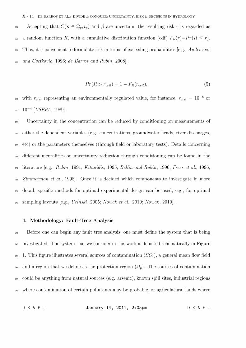
Before one can begin any fault tree analysis, one must define the system that is being241

investigated. The system that we consider in this work is depicted schematically in Figure242

1. This figure illustrates several sources of contamination (SOi), a general mean flow field243

and a region that we define as the protection region (Ωp). The sources of contamination244

could be anything from natural sources (e.g. arsenic), known spill sites, industrial regions245

where contamination of certain pollutants may be probable, or agriculatural lands where246

D R A F T January 14, 2011, 2:05pm D R A F T

DE BARROS ET AL.: DIVIDE & CONQUER: UNCERTAINTY, RISK & DECISIONS IN HYDROLOGY X - 15

certain contaminants may occur, to any other imaginable source of contamination. Sim-247

ilarly the protection zone could be anything like a well field, a lake or a residential area.248

The system defined in this work is deliberately kept generic and would of course be made249

more specific to a particular problem under consideration as the demand arises. Based250

on this generic system, we will follow the six steps outlined in the introduction. We will251

present a more specific illustrative example in the following section.252

Step 1: Defining System Failure253

We define failure of this system (SF ) when risk, as defined in section 3, exceeds a critical254

regulatory value:255

SF : r > rcrit (6)

with exceedance probability given by Eq (5).256

Step 2: Identifying the Key Components/Events257

We use this particular step to divide the problem into two components: A hydrologi-258

cal contamination scenario and the consequences of contamination on human health risk.259

This is an important distinction because concentration exceedance does not imply that260

the population is at risk. For example, individuals not drinking tap water (or with ex-261

ceptional physiology) might be at little or no risk. For such reasons, the combination of262

the concentration and the health parameters is the important factor to consider (only the263

joint effect can culminate in adverse health effects).264

D R A F T January 14, 2011, 2:05pm D R A F T

X - 16 DE BARROS ET AL.: DIVIDE & CONQUER: UNCERTAINTY, RISK & DECISIONS IN HYDROLOGY

The first key component follows a similar path to the works of Tartakovsky [2007],265

Winter and Tartakovsky [2008] and Bolster et al. [2009]. It focuses on the hydrological266

component and is meant to establish whether it is necessary at all to consider health risk.267

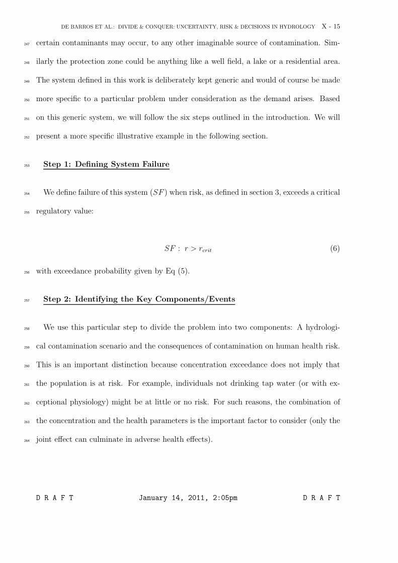
This event is called “Critical Concentration of Exposure ”(CCEi) and is defined as the268

event that the concentration of a contaminant i, arriving at the protection zone, exceeds269

some critical concentration value. If such an event occurs, decision makers must be alerted270

and should become concerned about the consequences on human health. The lower-level271

events associated with this key event are:272

SOi (Source Occurrence) is the event that a contaminant exists. In many possible273

scenarios, the existence of a contaminant source is not deterministic. For instance, a274

contamination source provenient from fertilizers or pesticides within an agricultural zone275

may (or may not) exist and the probability of its occurrence must be quantified.276

P1,i (Plume Path 1) is the event that the plume evolving from contaminant source i277

bypasses the protection zone.278

P2,i (Plume Path 2) refers to the event that the same plume hits the protection zone.279

If such a path does not exist, due to the morphology of the hydrosystem, then there is no280

reason for concern281

NAi (Natural Attenuation) represents the event that natural attenuation can decrease282

concentration peaks below a defined threshold value through chemical reactions, dispersion283

and dilution.284

D R A F T January 14, 2011, 2:05pm D R A F T

DE BARROS ET AL.: DIVIDE & CONQUER: UNCERTAINTY, RISK & DECISIONS IN HYDROLOGY X - 17

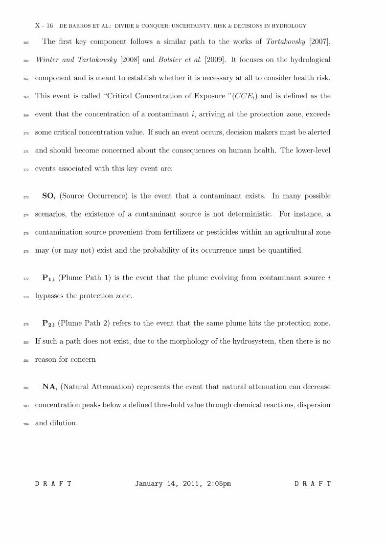
The second component relates to all health risk considerations. For this component,285

the basic events are:286

CCEi (Critical Concentration of Exposure) reflects the concentration that, when com-287

bined to a value β (see the relation in Eq. 2), will result in risk exceeding its critical value288

established by regulations (e.g., rcrit = 10−6 or 10−4), i.e., system failure will occur.289

BPCi (Behavioral Physiological Component) corresponds to the event that an individ-290

ual (or population cohort) that is exposed has characteristic β (see Eq. 3).291

The point to note here is that CCEi is conditioned on a value of β provenient from292

BPCi, which, as highlighted in section 3, is not a single value and it varies within the293

population based on several parameters [e.g., Maxwell et al., 1998; Maxwell and Kasten-294

berg , 1999; Maxwell et al., 1999; de Barros and Rubin, 2008; de Barros et al., 2009]. As295

expressed in Equation (4), each individual contains a specific β (e.g., jth individual with296

characteristic βj). The fact that CCEi can be defined only for a given value of β will re-297

quire, in a later stage of our analysis, an extension of the conventional fault tree approach298

to account for all possible values from the distribution of β.299

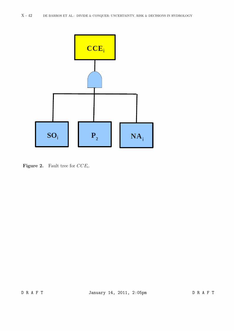
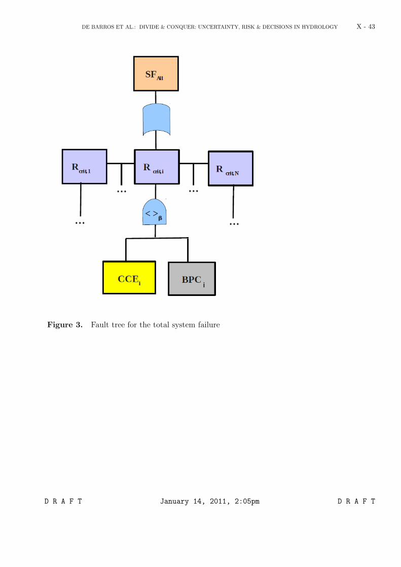
Step 3: Building the Fault Tree(s)300

In step 2, we divided the problem into two sections. In this step we will draw a fault tree301

for each of those sections. The first branch of the fault tree addresses the hydrogeological302

contamination scenario, leading to the key event CCEi. The fault tree is shown in Figure303

2 and is, in some sense, a version of the fault tree discussed in Bolster et al. [2009]. The304

combination with the second branch yields the main fault tree and represents the novelty305

D R A F T January 14, 2011, 2:05pm D R A F T

X - 18 DE BARROS ET AL.: DIVIDE & CONQUER: UNCERTAINTY, RISK & DECISIONS IN HYDROLOGY

of this work. This main fault tree replicates for each contaminant species and source and306

is shown in Figure 3. It illustrates visually how we have linked contamination and human307

health risk. The system failure (risk exceedance) for contaminant i is the joint occurrence308

of the events CCEi and BPCi.309

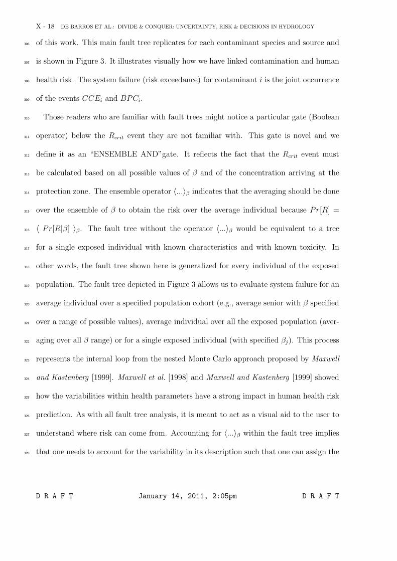
Those readers who are familiar with fault trees might notice a particular gate (Boolean310

operator) below the Rcrit event they are not familiar with. This gate is novel and we311

define it as an “ENSEMBLE AND”gate. It reflects the fact that the Rcrit event must312

be calculated based on all possible values of β and of the concentration arriving at the313

protection zone. The ensemble operator 〈...〉β indicates that the averaging should be done314

over the ensemble of β to obtain the risk over the average individual because Pr[R] =315

〈 Pr[R|β] 〉β. The fault tree without the operator 〈...〉β would be equivalent to a tree316

for a single exposed individual with known characteristics and with known toxicity. In317

other words, the fault tree shown here is generalized for every individual of the exposed318

population. The fault tree depicted in Figure 3 allows us to evaluate system failure for an319

average individual over a specified population cohort (e.g., average senior with β specified320

over a range of possible values), average individual over all the exposed population (aver-321

aging over all β range) or for a single exposed individual (with specified βj). This process322

represents the internal loop from the nested Monte Carlo approach proposed by Maxwell323

and Kastenberg [1999]. Maxwell et al. [1998] and Maxwell and Kastenberg [1999] showed324

how the variabilities within health parameters have a strong impact in human health risk325

prediction. As with all fault tree analysis, it is meant to act as a visual aid to the user to326

understand where risk can come from. Accounting for 〈...〉β within the fault tree implies327

that one needs to account for the variability in its description such that one can assign the328

D R A F T January 14, 2011, 2:05pm D R A F T

DE BARROS ET AL.: DIVIDE & CONQUER: UNCERTAINTY, RISK & DECISIONS IN HYDROLOGY X - 19

probability of occurrence for the event Rcrit. The “ENSEMBLE AND”gate generalizes329

the previous fault tree by covering over all range of population behavioral characteristics.330

Step 4: Translation to Boolean Logic331

This part can be viewed as the final stage in the development of the risk assessment332

system. The subsequent steps (items 5 and 6 in the introduction) involve the actual333

calculations of probabilities of all basic events and the combination thereof based on334

the expression that emerges from the current step. First, we will write a Boolean logic335

expression for the probability of event CCEi occurring. The “AND”and “OR”operators336

represents multiplications and additions of probabilities respectively. As discussed (and337

as can be seen from the fault tree in Figure 2), the appropriate Boolean expression for338

failure CCEi is given by339

CCEi = SOi AND P2,i AND NAi, (7)

with probability of occurrence:340

Pr[CCEi] = Pr[SOi] Pr[P2,i] Pr[NAi], (8)

since SOi, P2,i and NAi are completely independent of each other. Similarly, for the main341

fault tree depicted in Figure 3, the Boolean expression for system failure associated with342

each source Rcrit,i can be written as343

Rcrit,i = CCEi AND BPC (9)

with probability of occurrence:344

D R A F T January 14, 2011, 2:05pm D R A F T

X - 20 DE BARROS ET AL.: DIVIDE & CONQUER: UNCERTAINTY, RISK & DECISIONS IN HYDROLOGY

Pr[Rcrit,i] = Pr[CCEi] Pr[BPC]. (10)

If more contaminants are present (i ≥ 2), then the total system failure (SFall) is given345

by:346

SFall = Rcrit,1 ORRcrit,2 OR...ORRcrit,N (11)

and the probability of system failure is given by

Pr[SFall] = Pr[SF1] + Pr[SF2] + ... + Pr[SFN ]. (12)

Steps 5 and 6, see Section 2, are straightfoward and need no further explanation. In347

the following section, we will develop them for an illustrative example.348

5. Illustrative Example

Our goal is to show how the methodology can accommodate the entire range from349

simple to complex problems and solution approaches. It is seldom that a large data350

set is available in probabilistic health risk assessment, and we cannot always solve the351

problem entirely. For such reasons, it is common to make conservative assumptions and352

assess the worst case scenario with simple models [Troldborg et al., 2009; Bolster et al.,353

2009]. The scenario under consideration assumes almost complete absence of site-specific354

data, leading to crude yet conservative estimates of probabilities. Other existing methods355

rather than the simple one we selected for the illustration here can be found in the356

literature, (e.g. see Rubin [2003] for an extensive review). The level of complexity in357

the analysis of each component and event can vary according to the available information358

and the importance within the fault tree, and can easily be adapted interactively during359

D R A F T January 14, 2011, 2:05pm D R A F T

DE BARROS ET AL.: DIVIDE & CONQUER: UNCERTAINTY, RISK & DECISIONS IN HYDROLOGY X - 21

the analysis. If hydrological field data is available and more complex physical-chemical360

processes are involved, one may opt for numerical Monte Carlo simulations to allow more361

flexibility in relaxing simplifying assumptions as done in Maxwell and Kastenberg [1999];362

Maxwell et al. [1999] and de Barros et al. [2009]. Without loss of generality, our illustrative363

example will focus in a groundwater contamination problem. The method shown here can364

also be applied to surface water bodies or to coupled catchment-scale problems [e.g.,365

Baresel and Destouni , 2007; Persson and Destouni , 2009].366

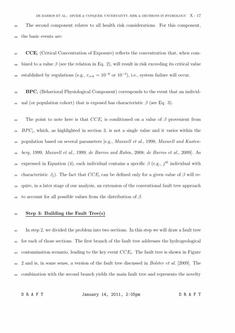
5.1. Physical Scenario and Assumptions

We consider a regional aquifer, confined, 2D depth-averaged with mean flow velocity367

U taken along the x-direction. A degrading contaminant is continuously released with368

inlet concentration Co within a rectangular source with transverse dimension w = ySR -369

ySL (see Figure 4). Once contamination has occurred, the contaminant plume might hit370

the environmentally sensitive target represented by a control plane (CP ) situated at a371

distance x = Lb - Ls from the source zone (see Figure 4). The schematic representation372

of the physical problem is given in Figure 4.373

At this stage, we will evaluate the concentration field under the worst case scenario.374

This is a common approach in human health risk assessment since decision makers must375

account for safety factors when dealing with human lives [Troldborg et al., 2008, 2009;376

McKnight et al., 2010]. We assume, in accordance with the worst case scenario philosophy,377

that the concentration can be calculated using a 1D solution by neglecting transverse378

dispersion between neighboring streamlines. Further more, longitudinal dispersion is also379

neglected. This excludes dilution processes as described by Kitanidis [1994]. The only380

D R A F T January 14, 2011, 2:05pm D R A F T

X - 22 DE BARROS ET AL.: DIVIDE & CONQUER: UNCERTAINTY, RISK & DECISIONS IN HYDROLOGY

natural attenuating factor is degradation with linear decay coefficient λ (neglecting pore-381

scale dispersion):382

C(τ) = Co exp[−λτ ], (13)

where τ = x/U denotes the travel time between source and control plane. In the sub-383

sequent sections, we will account for the uncertainty in τ in order to derive a simple384

expression for the concentration probability density function (pdf) and λ is known.385

5.2. Quantifying Probabilities of Occurrence

5.2.1. Probability of Travel Paths386

Here we compute the probabilities of path 1 or 2 of occurring, i.e. events P1 and P2 (see387

Section 4 for definitions). We prefer to calculate the probability of the plume bypassing388

the control plane (Pr[P1]). Since Pr[P1] and Pr[P2] are mutually exclusive, we have:389

Pr[P2] = 1 − Pr[P1]. (14)

In order to compute the above probabilities, we must quantify the pdf of each contami-390

nant particle within the source zone intercepting the control plane of the protection zone.391

Neglecting pore-scale dispersion (both longitudinal and transverse), we approximate the392

time of interception tb by the mean travel time tb ≈ Lb−Ls

U(time from the source to the393

control plane). In analogy to the work presented in Bolster et al. [2009], we assume a394

Gaussian model to describe the particle displacement pdf. For alternative definitions of395

the displacement pdf, we refer to Dagan [1987]; Rubin [2003]. Our resulting pdf is given396

by:397

D R A F T January 14, 2011, 2:05pm D R A F T

DE BARROS ET AL.: DIVIDE & CONQUER: UNCERTAINTY, RISK & DECISIONS IN HYDROLOGY X - 23

p1(Lb, tb) =1√

4πDefftbe−

(yb−yo)2

4Deff tb , (15)

where yo is a point within the contamination zone. Deff is an effective macroscopic dis-398

persion coefficient (purely uncertainty-related) that can arise for a variety of reasons, e.g.,399

due to heterogeneity [Dagan, 1989; Rubin, 2003] or due to temporal fluctuations in the400

flow field [Dentz and Carrera, 2005] to mention but a few. Accounting for a dispersive401

term in Eq. (15), but not in Eq. (13), might seem inconsistent at first sight, but it is a402

consistent set of worst-case assumptions.403

If no particles from the source bypasses the control plane either on the left or on the right,404

then no interception occurs. A conservative envelope can be constructed by considering405

that particles from the back right point [sR = (Ls, ysR)], see Figure 4, have to pass by the406

outer left point of the protection zone [bL = (Lb, ybL)] and vice-versa.407

Pr(P1) = Pr(P1,L) + Pr(P1,R)

=

∫ ybL

−∞

1√

4πDeff tbe−

(yb−ysR)2

4Deff tb dyb

+

∫

∞

ybRy

1√

4πDeff tbe−

(yb−ysL)2

4Deff tb dyb. (16)

5.2.2. Probability of Natural Attenuation408

Above, we used the back end of the source as worst case scenario for interception with409

the protection zone. The worst case scenario for natural attenuation is based on the front410

center of the source area because this yields the shortest distance (thus shortest time) for411

decay.412

D R A F T January 14, 2011, 2:05pm D R A F T

X - 24 DE BARROS ET AL.: DIVIDE & CONQUER: UNCERTAINTY, RISK & DECISIONS IN HYDROLOGY

Given the uncertainty in flow parameters and scarce site characterization, we con-413

sider for illustration the travel time τ to be stochastic and lognormally distributed [e.g.,414

Cvetkovic et al., 1992]:415

fτ (τ) =e−

(log(τ)−µτ )2

2σ2τ

√2πσττ

, (17)

with µτ and στ denoting the travel time mean and variance in logarithmic space and are416

related to the mean velocity [e.g., Andricevic et al., 1994].417

We can now calculate the pdf for concentration based on the travel time pdf and Eq.

(13):

fc(C) =

∣

∣

∣

∣

dτ

dC

∣

∣

∣

∣

fτ (τ), (18)

which allows us to evaluate the probability of the concentration being above a regulatory

threshold value Ccrit at the sensitive target. Substituting Eq. (13) into Eq. (18), we

obtain:

fc(C) =1

λCfτ

(

1

λln

[

C

Co

])

, (19)

Eq. (18) reflects only one possible and simple choice of model for the concentration pdf418

under the conditions assumed in the current work for illustrative purposes. It is worth419

mentioning that many other models could be used in this approach under more generic420

conditions [e.g., Rubin et al., 1994; Bellin and Tonina, 2007; Cirpka et al., 2008]. For421

example, other choices for travel time distributions can be found in Ch. 10 of Rubin422

[2003] and in Sanchez-Vila and Guadagnini [2005]. If hydrogeological data is available,423

one could also follow the approach described in Rubin and Dagan [1992] to condition the424

travel time pdf.425

5.2.3. Probability of Risk Exceedence426

D R A F T January 14, 2011, 2:05pm D R A F T

DE BARROS ET AL.: DIVIDE & CONQUER: UNCERTAINTY, RISK & DECISIONS IN HYDROLOGY X - 25

Based on Eq. (5), we can evaluate the probability that the risk will exceed a threshold427

value rcrit. Here, we present a risk distribution for the commonly used risk model given428

in Eq. (2). In order to evaluate the risk cdf (FR) based on the pdf fβ of the health429

parameters and concentration pdf fC we have:430

FR(rcrit) =

∫ rcrit

0

∫

∞

0

fβ(β)fC

(

r

β

)

1

βdrdβ (20)

where we used statistical independence between β and C. The concentration pdf comes431

from Eq. (18) while fβ is determined from population studies [e.g., Dawoud and Purucker ,432

1996] or the data provided in Maxwell et al. [1998] and Benekos et al. [2007]. If a single433

individual with characteristics βo is exposed, then Eq. (20) becomes:434

FR(rcrit) =

∫ rcrit

0

∫

∞

0

δ(β − βo)fC

(

r

β

)

1

βdrdβ

FR(rcrit) =1

βo

∫ rcrit

0

fC

(

r

βo

)

dr, (21)

where we used the properties of the Dirac Delta δ: fβ(β) = δ(β − βo). This feature is435

incorporated in the fault tree represented in Figure 3 and illustrates how the approach can436

be used to cover cases for a single exposed individual and for a fully exposed population437

(also different population cohorts: gender and/or age dependent).438

6. Results and Discussion

We illustrate the methodology by considering a simple example for cancer risk. Two439

species (A and B) are continuously released from their source locations and may pose440

a threat to human lives. The two contaminants are released in different locations, with441

different source dimensions and initial concentrations (to reproduce the varying range of442

D R A F T January 14, 2011, 2:05pm D R A F T

X - 26 DE BARROS ET AL.: DIVIDE & CONQUER: UNCERTAINTY, RISK & DECISIONS IN HYDROLOGY

typical situations found in the field). Both contaminants are released from line sources443

with dimensions 4 m (for contaminant A) and 2 m (for contaminant B). Contaminant A444

is closer to the protection zone (35 m) while contaminant B is further away (60 m). These445

values as well as other relevant parameters are summarized in Table 1. The main sources446

of uncertainty under consideration here are the contaminant travel times, Eq. (17). We447

also account for the variability in the health-related parameter β, Eq. (3). For the current448

scenario, we assume that travel time standard deviation is equal to στ = 0.1 d and that449

Deff = 0.1 m2/d.450

Since we have two distinct contaminants, the values for β are different. For instance,451

contaminant A affects a specific population cohort while contaminant B affects a different452

one (thus reflecting variability). In this example, we assume both values of β to be453

lognormally distributed with mean µlnβ and standard deviation σlnβ, see Table 1 (values454

given in logarithmic space). Figure 5 illustrates the pdf of β for contaminants A and B.455

Risk estimates were obtained using the linear model in Eq. (2) and their corresponding456

probabilities of exceeding a regulatory value are computed through the cdf provided in457

Eq. (20).458

Given that contamination is known to exist (SO with probability 1), we need to evaluate459

the probabilities associated with each branch of the fault tree using the steps described460

in Section 4. The events and their corresponding probabilities are summarized in Table 2461

for both contaminants.462

With the data given in Table 1 and using Eq. (16), the probability of the plume463

hitting the sensitive target is Pr[P2] = 0.38 for contaminant A and Pr[P2]= 0.26 for464

contaminant B. From the results given in Figure 6, we can also extract the probabilities465

D R A F T January 14, 2011, 2:05pm D R A F T

DE BARROS ET AL.: DIVIDE & CONQUER: UNCERTAINTY, RISK & DECISIONS IN HYDROLOGY X - 27

of the concentration being above a regulatory threshold value Ccrit. The probabilities of C466

≥ Ccrit for contaminant A is 0.18 where for contaminant B we have 0.015. This is caused467

by the physical setup of the problem, since the source for contaminant A is closer to the468

environmentally sensitive target than to the release location of contaminant B. This shows469

how the extension of the contaminant source as well as its distance from the protection470

zone influences the probabilities of the plume hitting the target and of the concentration471

exceedance.472

Figure 7 depicts the risk cdfs for both contaminants. Assuming that the critical risk473

value established by the regulatory agency is rcrit = 10−4, we can compute the risk ex-474

ceedance probabilities Pr(R > rcrit) using Eq. (5), and obtain 0.69 and 0.54 for species475

A and B respectively. With Eq. (10), the probability of system failure can be obtained476

(values given in Table 2).477

Next, we illustrate a sensitivity analysis to identify which parameters are more relevant478

in predicting the system failure for contaminants A and B. In addition, it serves as a first479

screening tool to see which parameters are dominant in each of the branches of the fault480

tree and may require more detailed investigation. The parameters chosen to perform the481

sensitivity analysis are θ = U , Deff , λ, σ, µln β, σln β . We perturb, one by one, each482

parameter within θ by 10 percent and re-evaluate the probability of system failure each483

time. The resulting differences (between the perturbed and unperturbed case) given by484

∆Pr[SF ] are depicted in Figures 8 and 9 for contaminants A and B, respectively.485

One striking difference between Figures 8 and 9 is the sensitivity of system failure to486

the health-related parameters: Contaminant A is more sensitive to the health-related487

parameters than contaminant B. This result aligns well with the results by de Barros488

D R A F T January 14, 2011, 2:05pm D R A F T

X - 28 DE BARROS ET AL.: DIVIDE & CONQUER: UNCERTAINTY, RISK & DECISIONS IN HYDROLOGY

and Rubin [2008]. They showed that the relative significance of health-related parameters489

decreases with travel distance, because of the uncertainty in transverse plume position490

increases [Rubin, 1991]. Moreover, we note that both contaminants respond differently to491

all other parameters, with the exception of the mean velocity.492

For contaminant A, the macroscopic effective dispersion parameter (Deff) is less impor-493

tant, see Figure 8, since the source area for contaminant A is close to the environmental494

target. Over short travel distances, the macroscopic effective dispersion has a small prob-495

ability to make the plume bypass the protection zone (event P2). Vice-versa, Deff has496

a larger significance in the probability of system failure for contaminant B, because its497

source is located farther away from the target (event P2).498

The decay coefficient, λ, is the second most important parameter relative to the others499

for contaminant A. Since the source for pollutant A is so close to the protection zone,500

decay is the only process that can significantly reduce the probability of system failure.501

The opposite occurs for contaminant B, since the significance of other events is higher.502

Figure 10 shows how the coefficients of variation of the statistical distribution of risk503

changes for each perturbation in θ. This quantifies how sensitive the uncertainty is in504

assessing health risk to each individual parameter. In the current simple example, λ and505

U have stronger effects on the uncertainty of risk for both species A and B than all other506

parameters. We also observe that the mean and standard deviation of the health-related507

component (µlnβ and σln β) has a significant contribution in the final risk pdf. These health508

parameters have a stronger contribution to the spread of the risk pdf for contaminant A509

(closer to the source) than for B. For predictions closer to the source, characterization510

of the health parameters becomes important since concentrations are still high. As the511

D R A F T January 14, 2011, 2:05pm D R A F T

DE BARROS ET AL.: DIVIDE & CONQUER: UNCERTAINTY, RISK & DECISIONS IN HYDROLOGY X - 29

distance between the contaminant source and receptor increases, the contaminant plume’s512

peak concentration decreases due to the physical processes involved (in our case, decay).513

Source dimensions and distance to the protection zone have a definite role in defining the514

significance of the health parameters in the final risk. Again, this agrees with the results515

from de Barros and Rubin [2008].516

Although we have used a simple linear dose-response curve to evaluate cancer risk for517

the illustration, many other alternatives exist with varying levels of uncertainty. For518

instance, the work of Yu et al. [2003] provides detailed epidemiological dose-response519

curves and parameter uncertainties for arsenic that are age- and gender-dependent. Such520

dose-response curves are less subject to uncertainty than cancer risk models, because the521

latter rely on extrapolated animal-to-human data. This implies that, if the a contaminant522

site has several contaminants, different types of risk models could be used. This would lead523

to different relative contributions to uncertainty propagation in assessing system failure524

as discussed in de Barros et al. [2009].525

An important and attractive feature of the methodology shown is that it allows one to526

observe, in a most graphical manner, the sensitivity of the probabilities in system failure527

for each branch of the tree. This is a crucial basis for supporting managing decisions. For528

example, it indicates how to allocate resources towards further site characterization via529

prioritization according to highest risk contributions and highest sensitivity.530

7. Summary and Conclusions

In this work, we used the fault tree methodology to evaluate human health risk in a531

probabilistic manner. The approach breaks complex problems into individual events that532

can be tackled individually. The main differences between the ideas proposed here and the533

D R A F T January 14, 2011, 2:05pm D R A F T

X - 30 DE BARROS ET AL.: DIVIDE & CONQUER: UNCERTAINTY, RISK & DECISIONS IN HYDROLOGY

previous works [Tartakovsky , 2007; Winter and Tartakovsky , 2008; Bolster et al., 2009]534

are:535

1. The fault tree proposed here accounts for the uncertainty in both hydrogeological536

and health component;537

2. System failure is defined in terms of risk being above a threshold value;538

3. We introduced of a new form of stochastic fault-tree that weakens the assumption539

of independent events which is necessary in conventional fault tree analysis.540

Although we used only a crude and simple setting to illustrate the methodology, the541

approach can be used with arbitrarily more complex models. However, such simple ap-542

proaches can be useful for performing a preliminary screening in PRA, see works by543

Troldborg et al. [2008, 2009]. For instance, with an initial estimate based on simple mod-544

els, one can identify the events which contribute most to the final risk estimate or those545

that propagate the highest degree of uncertainty throughout the system. This information546

can then be used to invest further resources to these specific events, and more elaborate547

models can be used if additional data becomes available. The divide & conquer and mod-548

ularity features of the proposed framework easily allow the methods or tools used in each549

component to be easily exchanged (and refined) in later analysis without being intrusive550

in other components.551

Moreover, assessing health-related risk in hydrosystems is an interdisciplinary field and552

it relies on the expertise from a large number of disciplines (for example, hydrologists,553

engineers, public health, etc). As a result, communicating the information across inter-554

faces between different fields in an efficient and comprehensible manner is needed such555

that reliable water management decisions are made. The divide and conquer approach556

D R A F T January 14, 2011, 2:05pm D R A F T

DE BARROS ET AL.: DIVIDE & CONQUER: UNCERTAINTY, RISK & DECISIONS IN HYDROLOGY X - 31

inherent to fault trees allows individual experts to work on the individual problems with557

clear communication interfaces given by the fault tree structure. The approach allows558

decision makers to better visualize the components culminating in system failure (e.g.,559

population at risk) as well as the uncertainty emerging from each subsystem. This is560

appealing from the decision maker’s perspective, since it does not require entering into561

the complex details of each component of the PRA and helps communicate probabilistic562

concepts to practioners. Furthermore, it acts as a translator to experts from different563

fields, thus aiding public authorities in policy making and water management.564

Despite the fact that our work focused on a groundwater contamination application,565

it can be also used in other problems such as soil contamination, well vulnerability and566

surface waters and catchment-scale coupled problems [e.g., Frind et al., 2006; Baresel and567

Destouni , 2007; Troldborg et al., 2008, 2009; Persson and Destouni , 2009]. Furthermore,568

an emerging challenge consists in using the ideas discussed in this paper to tackle a fully569

integrated hydrosystem (groundwater, soil, surface water, etc.) where the need for divid-570

ing a complicated problem into smaller ones as well as interdisciplinary communication571

are even more evident [Persson and Destouni , 2009; McKnight et al., 2010]. For instance,572

Bertuzzo et al. [2008] studied how river networks (acting as environmental corridors) af-573

fect the spreading of cholera epidemics. These authors clearly showed how hydrological,574

health and demographical data needs to be considered in order to capture an accurate575

description of the main controlling factors dictating the spread of cholera epidemics.576

As pointed out in the literature, practitioners are still reluctant to embrace the concepts577

of uncertainty [Pappenberger and Beven, 2006]. Such resistance has also been a matter578

of discussion in a 2004 Forum published in Stochastic Environmental Research and Risk579

D R A F T January 14, 2011, 2:05pm D R A F T

X - 32 DE BARROS ET AL.: DIVIDE & CONQUER: UNCERTAINTY, RISK & DECISIONS IN HYDROLOGY

Assessment [Christakos, 2004; Freeze, 2004; Rubin, 2004]. A common conclusion is that580

the dialogue between the interdisciplinary groups is of utmost importance. Thus, having a581

tool that allows to illustrate, in a rather simplistic manner, these concepts (uncertainties)582

and its impact on society (for example, through risk) provides a step towards strengthening583

the bridge between the scientific developments in stochastic hydrogeology and the state-584

of-practice.585

Acknowledgments. The first and fourth authors would like to thank the German586

Research Foundation (DFG) for financial support of the project within the Cluster of587

Excellence in Simulation Technology (EXC310/1) at the University of Stuttgart. This588

work has been partially supported by the Spanish Ministry of Science and Innovation589

through projects RARA AVIS (reference CGL2009-11114) and Consolider-Ingenio 2010590

(ref. CSD2009-00065). We also would like acknowledge the comments made by our591

reviewers.592

References

Andricevic, R., and V. Cvetkovic (1996), Evaluation of Risk from Contaminants Migrating593

by Groundwater, Water Resources Research, 32 (3), 611–621.594

Andricevic, R., J. Daniels, and R. Jacobson (1994), Radionuclide migration using travel595

time transport approach and its application in risk analysis, Journal of Hydrology, 163,596

125–145.597

Baresel, C., and G. Destouni (2007), Uncertainty-accounting environmental policy and598

management of water systems, Environ. Sci. Technol, 41 (10), 3653–3659.599

D R A F T January 14, 2011, 2:05pm D R A F T

DE BARROS ET AL.: DIVIDE & CONQUER: UNCERTAINTY, RISK & DECISIONS IN HYDROLOGY X - 33

Bedford, T., and R. Cooke (2003), Probalistic Risk Analysis: Foundations and Methods,600

Cambridge University Press.601

Bellin, A., and Y. Rubin (1996), HYDRO GEN: A spatially distributed random field602

generator for correlated properties, Stochastic Hydrology and Hydraulics, 10 (4), 253–603

278.604

Bellin, A., and D. Tonina (2007), Probability density function of non-reactive solute con-605

centration in heterogeneous porous formations, Journal of contaminant hydrology, 94 (1-606

2), 109–125.607

Benekos, I., C. A. Shoemaker, and J. R. Stedinger (2007), Probabilistic risk and uncer-608

tainty analysis for bioremediation of four chlorinated ethenes in groundwater, Stochastic609

Environmental Research Risk Assessment, 21, 375–390.610

Benson, D. A., and M. M. Meerschaert (2008), Simulation of chemical reaction via particle611

tracking: Diffusion-limited versus thermodynamic rate-limited regimes, Water Resour.612

Res., 44, W12,201, doi:10.1029/2008WR007,111.613

Bertuzzo, E., S. Azaele, A. Maritan, M. Gatto, I. Rodriguez-Iturbe, and A. Rinaldo614

(2008), On the space-time evolution of a cholera epidemic, Water Resources Research,615

44 (1), 1–W01,424.616

Bogen, K. T., and R. C. Spear (1987), Integrating Uncertainty and Interindividual Vari-617

ability in Environmental Risk Assessment, Risk Analysis, 7 (4), 427–436.618

Bolster, D., M. Barahona, M. Dentz, D. Fernandez-Garcia, X. Sanchez-Vila, P. Trinchero,619

C. Valhondo, and D. Tartakovsky (2009), Probabilistic risk analysis of groundwater620

remediation strategies, Water Resources Research, 45 (6).621

D R A F T January 14, 2011, 2:05pm D R A F T

X - 34 DE BARROS ET AL.: DIVIDE & CONQUER: UNCERTAINTY, RISK & DECISIONS IN HYDROLOGY

Bolster, D., D. A. Benson, T. LeBorgne, and M. Dentz (2010), Anomalous mixing and622

reaction induced by super-diffusive non-local transport, Physical Review E, Submitted.623

Burmaster, D., and A. Wilson (1996), An introduction to second-order random variables624

in human health risk assessments, Human and Ecological Risk Assessment: An Inter-625

national Journal, 2 (4), 892–919.626

Christakos, G. (2004), A sociological approach to the state of stochastic hydrogeology,627

Stochastic Environmental Research and Risk Assessment, 18 (4), 274–277.628

Cirpka, O., R. Schwede, J. Luo, and M. Dentz (2008), Concentration statistics for mixing-629

controlled reactive transport in random heterogeneous media, Journal of contaminant630

hydrology, 98 (1-2), 61–74.631

Cvetkovic, V., A. Shapiro, and G. Dagan (1992), A solute flux approach to transport632

in heterogenous formations 2: Uncertainty Analysis, Water Resources Research, 28 (5),633

1377–1388.634

Dagan, G. (1987), Theory of Solute Transport by Groundwater, Annual Review of Fluid635

Mechanics, 19, 183–215.636

Dagan, G. (1989), Flow and Transport in Porous Formations, Springer Verlag, Berlin.637

Davison, A., G. Howard, M. Stevens, P. Callan, L. Fewtrell, D. Deere, and J. Bartram638

(2005), Water Safety Plans Managing drinking-water quality from catchment to con-639

sumer. Geneva: World Health Organisation, Tech. rep., WHO/SDE/WSH/05.06.640

Dawoud, E., and S. Purucker (1996), Quantitative Uncertainty Analysis of Superfund641

Residential Risk Pathway Models for Soil and Groundwater: White Paper, Tech. rep.642

de Barros, F. P. J., and Y. Rubin (2008), A Risk-Driven Approach for643

Subsurface Site Characterization, Water Resources Research, 44 (W01414),644

D R A F T January 14, 2011, 2:05pm D R A F T

DE BARROS ET AL.: DIVIDE & CONQUER: UNCERTAINTY, RISK & DECISIONS IN HYDROLOGY X - 35

doi:10.1029/2007WR006,081.645

de Barros, F. P. J., Y. Rubin, and R. Maxwell (2009), The concept of comparative in-646

formation yield curves and its application to risk-based site characterization, Water647

Resources Research, 45 (W06401), doi:10.1029/2008WR007,324.648

Dentz, M., and J. Carrera (2005), Effective solute transport in temporally fluctuating flow649

through heterogeneous media, Water Resources Research, 41 (8), W08,414.650

Donado, L. D., X. Sanchez-Vila, M. Dentz, J. Carrera, and D. Bolster (2009), Multicom-651

ponent reactive transport in multicontinuum media, Water Resour. Res., 45, W11,402,652

doi:10.1029/2008WR006,823.653

Edery, Y., H. Scher, and B. Berkowitz (2009), Modeling bimolecular reactions and trans-654

port in porous media, Geophys. Res. Lett., 36, L02,407 doi:10.1029/2008GL036,381.655

Fiori, A., I. Jankovic, G. Dagan, and V. Cvetkovic (2007), Ergodic transport through656

aquifers of non-Gaussian log conductivity distribution and occurrence of anomalous657

behavior, Water Resources Research, 43 (9), W09,407.658

Fjeld, R., N. Eisenberg, and K. Compton (2007), Quantitative Environmental Risk Anal-659

ysis for Human Health, first ed., Wiley.660

Freer, J., K. Beven, and B. Ambroise (1996), Bayesian estimation of uncertainty in runoff661

prediction and the value of data: An application of the GLUE approach, Water Re-662

sources Research, 32 (7), 2161–2173.663

Freeze, R. (2004), The role of stochastic hydrogeological modeling in real-world engi-664

neering applications, Stochastic Environmental Research and Risk Assessment, 18 (4),665

286–289.666

D R A F T January 14, 2011, 2:05pm D R A F T

X - 36 DE BARROS ET AL.: DIVIDE & CONQUER: UNCERTAINTY, RISK & DECISIONS IN HYDROLOGY

Frind, E. O., J. W. Molson, and D. L. Rudolph (2006), Well vulnerability: a quantitative667

approach for source water protection, Ground water, 44 (5), 732–742.668

Gelhar, L. W., C. Welty, and K. Rehfeldt (1992), A critical review of data on field scale669

disperion in aquifers, Water Resour. Res, 28, 1955–1974.670

Gramling, C., C. Harvey, and L. Meigs (2002), Reactive transport in porous media: A671

comparison of model prediction with laboratory visualization, Environ. Sci. Technol.,672

36, 2508–2514.673

Kitanidis, P. (1994), The concept of the dilution index, Water Resources Research, 30 (7),674

2011–2026.675

Kitanidis, P. K. (1995), Quasi-linear geostatistical theory for inversing, Water Resour.676

Res., 31 (10), 2411–2419.677

Levy, M., and B. Berkowitz (2003), Measurement and analysis of non-fickian dispersion678

in heterogeneous porous media, Journal of Contaminant Hydrology, 64, 203–226.679

Maddalena, R. L., and T. E. McKone (2002), Developing and Evaluating Distributions680

for Probabilistic Human Exposure Assessments, Tech. Rep. LBNL-51492.681

Maxwell, R., and W. Kastenberg (1999), Stochastic Environmental Risk Analysis: An682

Integrated Methodology for Predicting Cancer Risk from Contaminated Groundwater,683

Stochastic Environmental Research Risk Assessment, 13, 27–47.684

Maxwell, R., S. Pelmulder, F. Tompson, and W. Kastenberg (1998), On the development685

of a new methodology for groundwater driven health risk assessment, Water Resources686

Research, 34 (4), 833–847.687

Maxwell, R., W. Kastenberg, and Y. Rubin (1999), A methodology to integrate site char-688

acterization information into groundwater-driven health risk assessment, Water Re-689

D R A F T January 14, 2011, 2:05pm D R A F T

DE BARROS ET AL.: DIVIDE & CONQUER: UNCERTAINTY, RISK & DECISIONS IN HYDROLOGY X - 37

sources Research, 35 (9), 2841–2885.690

Maxwell, R., S. Carle, and A. Tompson (2008), Contamination, Risk, and Heterogeneity:691

On the Effectiveness of Aquifer Remediation, Environmental Geology, 54, 1771–1786.692

McKnight, U., S. Funder, J. Rasmussen, M. Finkel, P. Binning, and P. Bjerg (2010), An693

integrated model for assessing the risk of TCE groundwater contamination to human694

receptors and surface water ecosystems, Ecological Engineering, In Press.695

McKone, T., and T. Bogen (1991), Predicting the uncertainties in risk assessment, Envi-696

ron. Sci. Technol., 25 (10), 1674–1681.697

McLucas, A. C. (2003), Decision making: risk management, systems thinking and situa-698

tion awareness, Argos Press, Canberra, Australia.699

Molin, S., and V. Cvetkovic (2010), Microbial risk assessment in heterogeneous aquifers:700

1. Pathogen transport, Water Resources Research, 46 (5 (W05518)).701

Molin, S., V. Cvetkovic, and T. Stenstrom (2010), Microbial risk assessment in heteroge-702

neous aquifers: 2. Infection risk sensitivity, Water Resources Research, 46 (5(W05519)).703

Morales, K. H., L. Ryan, T. L. Kuo, M. Wu, and C. J. Chen (2000), Risk of Internal704

Cancers from Arsenic in Drinking Water, Environmental Health Perspectives, 108 (7),705

655–661.706

Neuman, S. P., and D. M. Tartakovsky (2009), Perspective on theories of anoma-707

lous transport in heterogeneous media, Adv. Water Resour., 32 (5), 670–680, doi:708

10.1016/j.advwatres.2008.08.005.709

Nowak, W. (2010), Measures of parameter uncertainty in geostatistical estimation and710

design, Mathematical Geosciences, 42 (2), 199–221.711

D R A F T January 14, 2011, 2:05pm D R A F T

X - 38 DE BARROS ET AL.: DIVIDE & CONQUER: UNCERTAINTY, RISK & DECISIONS IN HYDROLOGY

Nowak, W., F. P. J. de Barros, and Y. Rubin (2010), Bayesian geostatistical design:712

Optimal site investigation when the geostatistial model is uncertain, Water Resour.713

Res., 46 (W03535), doi:10.1029/2009WR008,312.714

Pappenberger, F., and K. Beven (2006), Ignorance is bliss: Or seven reasons not to use715

uncertainty analysis, Water Resources Research, 42 (5), W05,302.716

Persson, K., and G. Destouni (2009), Propagation of water pollution uncertainty and risk717

from the subsurface to the surface water system of a catchment, Journal of Hydrology,718

377 (3-4), 434–444.719

Raje, D., and V. Kapoor (2000), Experimental study of bimolecular reaction kinetics in720

porous media, Environ. Sci. Technol., 24, 1234–1239.721

Rubin, Y. (1991), Prediction of tracer plume migration in heterogeneous porous media by722

the method of conditional probabilities, Water Resour. Res., 27 (6), 1291–1308.723

Rubin, Y. (2003), Applied Stochastic Hydrogeology, first ed., Oxford Press.724

Rubin, Y. (2004), Stochastic hydrogeology - challenges and misconceptions, Stochastic725

Environmental Research Risk Assessment, 18, 280–281.726

Rubin, Y., and G. Dagan (1992), Conditional estimates of solute travel time in heteroge-727

nous formations: impact of transmissivity measurements, Water Resources Research,728

28 (4), 1033–1040.729

Rubin, Y., M. A. Cushey, and A. Bellin (1994), Modeling of transport in groundwater for730

environmental risk assessment, Stochastic Hydrol. Hydraul., 8 (1), 57–77.731

Sanchez-Vila, X., and A. Guadagnini (2005), Travel time and trajectory moments of con-732

servative solutes in three dimensional heterogeneous porous media under mean uniform733

flow, Advances in Water Resources, 28, 429–439.734

D R A F T January 14, 2011, 2:05pm D R A F T

DE BARROS ET AL.: DIVIDE & CONQUER: UNCERTAINTY, RISK & DECISIONS IN HYDROLOGY X - 39

Sidle, C. R., B. Nilson, M. Hansen, and J. Fredericia (1998), Spatially varying hydraulic735

and solute transpiort characteristics of a fractured till determined by field tracer test,736

funen, denmark, Water Resour. Res, 34, 2515–2527.737

Silliman, S. E., L. Konikow, and C. Voss (1997), Laboratory experiment of longitudinal738

dispersion in anisotropic porous media, Water Resour. Res, 23, 2145–2154.739

Tartakovsky, D. (2007), Probabilistic risk analysis in subsurface hydrology, Geophysical740

Research Letters, 34 (5), 5404.741

Tartakovsky, D. M., and C. L. Winter (2008), Uncertain future of hydrogeology, ASCE742

J. Hydrologic Engrg., 13 (1), 37–39.743

Troldborg, M., G. Lemming, P. Binning, N. Tuxen, and P. Bjerg (2008), Risk assessment744

and prioritisation of contaminated sites on the catchment scale, Journal of contaminant745

hydrology, 101 (1-4), 14–28.746

Troldborg, M., P. Binning, S. Nielsen, P. Kjeldsen, and A. Christensen (2009), Unsat-747

urated zone leaching models for assessing risk to groundwater of contaminated sites,748

Journal of contaminant hydrology, 105 (1-2), 28–37.749

Ucinski, D. (2005), Optimal measurement methods for distributed parameter system iden-750

tification, CRC.751

USEPA (1989), Risk Assessment Guidance for Superfund Volume 1: Human Health Man-752

ual (Part A), Tech. Rep. Rep.EPA/540/1-89/002.753

USEPA (1991), Risk Assessment Guidance for Superfund Volume 1: Human Health Eval-754

uation (Part B), Tech. Rep. Rep.EPA/540/R-92/003.755

USEPA (2001), Risk Assessment Guidance for Superfund: Volume III - Part A, Process756

for Conducting Probabilistic Risk Assessment, Tech. Rep. Rep.EPA 540/R-02/002.757

D R A F T January 14, 2011, 2:05pm D R A F T

X - 40 DE BARROS ET AL.: DIVIDE & CONQUER: UNCERTAINTY, RISK & DECISIONS IN HYDROLOGY

Winter, C., and D. Tartakovsky (2008), A reduced complexity model for probabilistic risk758

assessment of groundwater contamination, Water Resources Research, 30 (6), 2799–759

2816.760

Yu, W., C. Harvey, and C. Harvey (2003), Arsenic in groundwater in Bangladesh: a761

geostatistical and epidemiological framework for evaluating health effects and potential762

remedies, Water Resources Research, 39 (6), 1146.763

Zimmerman, D. A., et al. (1998), A comparison of seven geostatistically based inverse ap-764

proaches to estimate transmissivities for modeling advective transport by groundwater765

flow, Water Resour. Res., 34 (6), 1373–1413.766

D R A F T January 14, 2011, 2:05pm D R A F T

DE BARROS ET AL.: DIVIDE & CONQUER: UNCERTAINTY, RISK & DECISIONS IN HYDROLOGY X - 41

SO

SO

SO

1

i

N

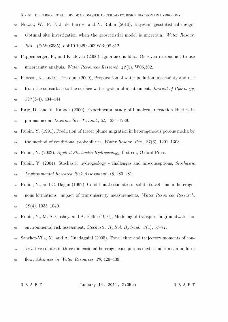
Figure 1. Schematic depiction of the contamination scenario considered in this work.

Several potential sources SOi, i = 1,...,N are considered. Each source implies the combi-

nation of a potentially hazard solute located in a given (sometimes unknown) location.

D R A F T January 14, 2011, 2:05pm D R A F T

X - 42 DE BARROS ET AL.: DIVIDE & CONQUER: UNCERTAINTY, RISK & DECISIONS IN HYDROLOGY

ii

i

Figure 2. Fault tree for CCEi.

D R A F T January 14, 2011, 2:05pm D R A F T

DE BARROS ET AL.: DIVIDE & CONQUER: UNCERTAINTY, RISK & DECISIONS IN HYDROLOGY X - 43

i

Figure 3. Fault tree for the total system failure

D R A F T January 14, 2011, 2:05pm D R A F T

X - 44 DE BARROS ET AL.: DIVIDE & CONQUER: UNCERTAINTY, RISK & DECISIONS IN HYDROLOGY

sR= (Ls, y

sR)s

L= (L

s, y

sL)

bL= (L

b, y

bL)

x

y

Contaminant Source Co

Protection Zone (or Control Plane) p

Mean Flow Direction

bR= (Lb, y

bR)

0

Figure 4. Schematic representation of the physical problem. A contaminant with initial

concentration Co is released. U is the mean velocity.

D R A F T January 14, 2011, 2:05pm D R A F T

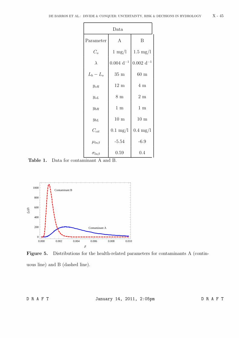
DE BARROS ET AL.: DIVIDE & CONQUER: UNCERTAINTY, RISK & DECISIONS IN HYDROLOGY X - 45

Data

Parameter A B

Co 1 mg/l 1.5 mg/l

λ 0.004 d−1 0.002 d−1

Lb − Ls 35 m 60 m

ysR 12 m 4 m

ysL 8 m 2 m

ybR 1 m 1 m

ybL 10 m 10 m

Ccit 0.1 mg/l 0.4 mg/l

µlnβ -5.54 -6.9

σlnβ 0.59 0.4

Table 1. Data for contaminant A and B.

Contaminant A

Contaminant B

0.000 0.002 0.004 0.006 0.008 0.010

0

200

400

600

800

1000

Β

f ΒHΒL

Figure 5. Distributions for the health-related parameters for contaminants A (contin-

uous line) and B (dashed line).

D R A F T January 14, 2011, 2:05pm D R A F T

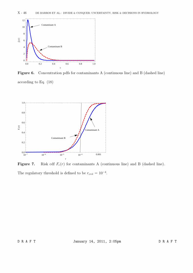
X - 46 DE BARROS ET AL.: DIVIDE & CONQUER: UNCERTAINTY, RISK & DECISIONS IN HYDROLOGY

Contaminant A

Contaminant B

0.0 0.2 0.4 0.6 0.8 1.0

0

2

4

6

8

10

12

c

f cHcL

Figure 6. Concentration pdfs for contaminants A (continuous line) and B (dashed line)

according to Eq. (18)

Contaminant A

Contaminant B

10-7 10-6 10-5 10-4 0.0010.0

0.2

0.4

0.6

0.8

1.0

r

FrH

rL

Figure 7. Risk cdf Fr(r) for contaminants A (continuous line) and B (dashed line).

The regulatory threshold is defined to be rcrit = 10−4.

D R A F T January 14, 2011, 2:05pm D R A F T

DE BARROS ET AL.: DIVIDE & CONQUER: UNCERTAINTY, RISK & DECISIONS IN HYDROLOGY X - 47

Probabilities

Event Parameter A B

SO Pr[SO] 1 1

P2 Pr[P2] 0.38 0.26

NA Pr(C ≥ Ccrit) 0.18 0.015

Rcrit Pr(r ≥ Rcrit) 0.69 0.54

SF Pr(SF ) 0.047 0.0022

Table 2. Computed probabilities for the hypothetical illustrative case

0.000

0.005

0.010

0.015

0.020

0.025

0.030

0.035

Pr

[SF]

lnlnD

effU

Sensitivity Analysis in System Failure for Contaminant A

Figure 8. Sensitivity analysis for contaminant A. Change in probability of system

failure ∆Pr[SF ] if each parameter in θ is perturbed by 10 percent.

D R A F T January 14, 2011, 2:05pm D R A F T

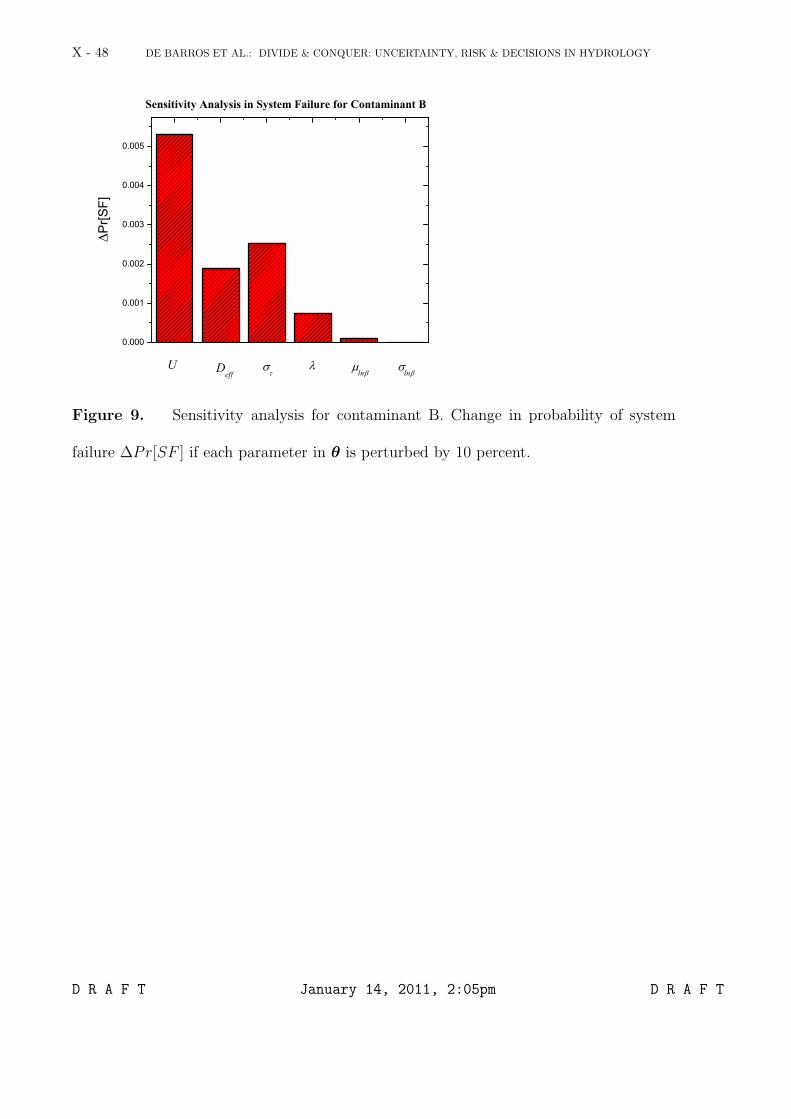
X - 48 DE BARROS ET AL.: DIVIDE & CONQUER: UNCERTAINTY, RISK & DECISIONS IN HYDROLOGY

0.000

0.001

0.002

0.003

0.004

0.005

Pr

[SF]

Sensitivity Analysis in System Failure for Contaminant B

lnlnDeff

U

Figure 9. Sensitivity analysis for contaminant B. Change in probability of system

failure ∆Pr[SF ] if each parameter in θ is perturbed by 10 percent.

D R A F T January 14, 2011, 2:05pm D R A F T

DE BARROS ET AL.: DIVIDE & CONQUER: UNCERTAINTY, RISK & DECISIONS IN HYDROLOGY X - 49

0.00

0.01

0.02

0.03

0.04

0.05

0.06

0.07

0.08

0.09 Contaminant B

lnlnDeff

U lnlnD

effU

CV

Contaminant A

Figure 10. The dependency of the risk coefficient of variation for contaminants A and

B on the perturbed parameter. Each parameter in θ was perturbed by 10 percent. The

coefficient of variation is equal to the risk standard deviation divided by its mean. Results

evaluated using Eq. 20. ∆CV corresponds to the change in the coefficient of variation.

D R A F T January 14, 2011, 2:05pm D R A F T