1

A distributional semantic approach to the periodization of change in the productivity of constructions

Florent Perek University of Birmingham

Martin Hilpert Université de Neuchâtel

This paper describes a method to automatically identify stages of language change in diachronic corpus data, combining variability-based neighbour clustering, which offers objective and reproducible criteria for periodization, and distributional semantics as a flexible and objective representation of lexical meaning. This method partitions the history of a grammatical construction according to qualitative stages of productivity corresponding to different sets of semantic classes attested in one of its lexical slots. Two case studies are presented. The first case study on the “Verb the hell out of NP” construction shows that the semantic development of a construction does not always match that of its quantitative aspects, like token or type frequency. The second case study on the way-construction compares the results of the present method with those of collostructional analysis. While the results overlap to some degree, it is shown that the former measures semantic change with greater precision, both regarding the nature of changes and their chronology. In sum, this method offers a promising exploratory approach to capturing variation in the semantic range of lexical fillers of constructions and to modeling constructional change.

1. Introduction: stages of language change Studies of language change typically describe diachronic developments in terms of discrete stages.1 For instance, while the shift from SOV to SVO word order in English was gradual, separate steps in this change have been identified: (i) SVO order in Old English initially involved auxiliaries only, which were displaced to second position in the clause for prosodic reasons, (ii) this innovation was extended to all finite verbs, but the SOV order persisted for some time, notably in dependent clauses, (iii) the SVO order was extended to all clauses, leading to the disappearance of SOV by the end of the Middle English period (Dewey 2006, Hock & Joseph 1996: 203-208).

The notion of periodization, i.e., identifying and dating stages of language change, can be applied to any aspect of the structure and usage of grammatical constructions. The process of identifying discrete stages in continuous diachronic variation is especially relevant for usage-based approaches to language change, in which change in the grammatical representation of linguistic generalizations is to be inferred from patterns of usage found in historical data. This issue is made all the more pressing by the wealth of data provided by the growing number of diachronic corpora and the increasing availability of tools to analyse this data.

Linguistic corpora can be divided into periods on the basis of different criteria. One possible yardstick is language-external history, which may contain watershed moments such as the Norman Conquest. Sometimes the limited availability of data constrains periodization. Some corpora are divided into time spans that reflect generational turnover. Which of these is best? This question was addressed by Gries & Hilpert (2008), who discuss the methodological issues that are implicated in a manual identification of stages. Emphasizing the need for an inductive and data- 1 We would like to thank Harald Baayen and one anonymous reviewer for their comments on an earlier version of this paper.

2

driven procedure, they introduce variability-based neighbour clustering (VNC) as a method for automatic corpus periodization. Unlike the periodization methods that were described above, VNC divides a diachronic corpus on the basis of data from the linguistic phenomenon that is being studied. As we will explain in more detail below, the method creates periods out of temporally adjacent data points that are similar in terms of one or more quantitative criteria. The output of VNC is a partition of the time scale into periods that are maximally coherent with respect to these criteria. Up to this point, VNC has been applied in studies that use token frequency, type frequency and other measures derived from them, or the frequency distribution of lexemes that are found with a given construction (cf. Gries & Hilpert 2010, Hilpert 2013). In this paper, we will extend the use of VNC to information that directly captures semantic dimensions of change, such as whether the construction is used with different semantic classes of lexical items. This kind of information is critical in particular for studies concerned with the productivity of grammatical constructions (e.g., Barðdal 2008, Colleman & De Clerck 2011, Israel 1996, Noël 2008, Noël & Colleman 2010).

In our extension of VNC, we draw on a distributional semantic model as a proxy to word meaning. Starting with the observation that words occurring in similar contexts tend to have similar meanings, distributional semantic representations approximate the meaning of a word by recording its co-occurrence with other words, usually in a large corpus (Turney & Pantel 2010). The present approach creates representations of constructional meaning in each time period from a distributional semantic model, and it uses these representations as input to VNC. We argue that our approach offers a promising addition to the range of available tools for quantitative studies of language change that sheds new light on the question of how constructions change in meaning and productivity.

This paper is structured as follows. Section 2 motivates and introduces VNC. Section 3 describes the variant of VNC used in this paper, with an explanation of how the distributional semantic model was created and used to generate the input to the VNC algorithm. Section 4 presents two case studies that illustrate how the method can capture changes in the productivity of constructions, thereby showing the benefits of using semantic information in VNC periodization.

2. Periodization and variability-based neighbour clustering Corpus-based studies of language change typically start with the extraction of tokens of interest from a diachronic corpus, possibly classifying these tokens according to some criterion, and using this data to compare language use at different points in time. When analysing quantitative trends, it is natural for researchers to try to describe them in terms of stages of language change, by assessing when this particular area of the language was relatively stable and for how long, and when it underwent change and in what direction.

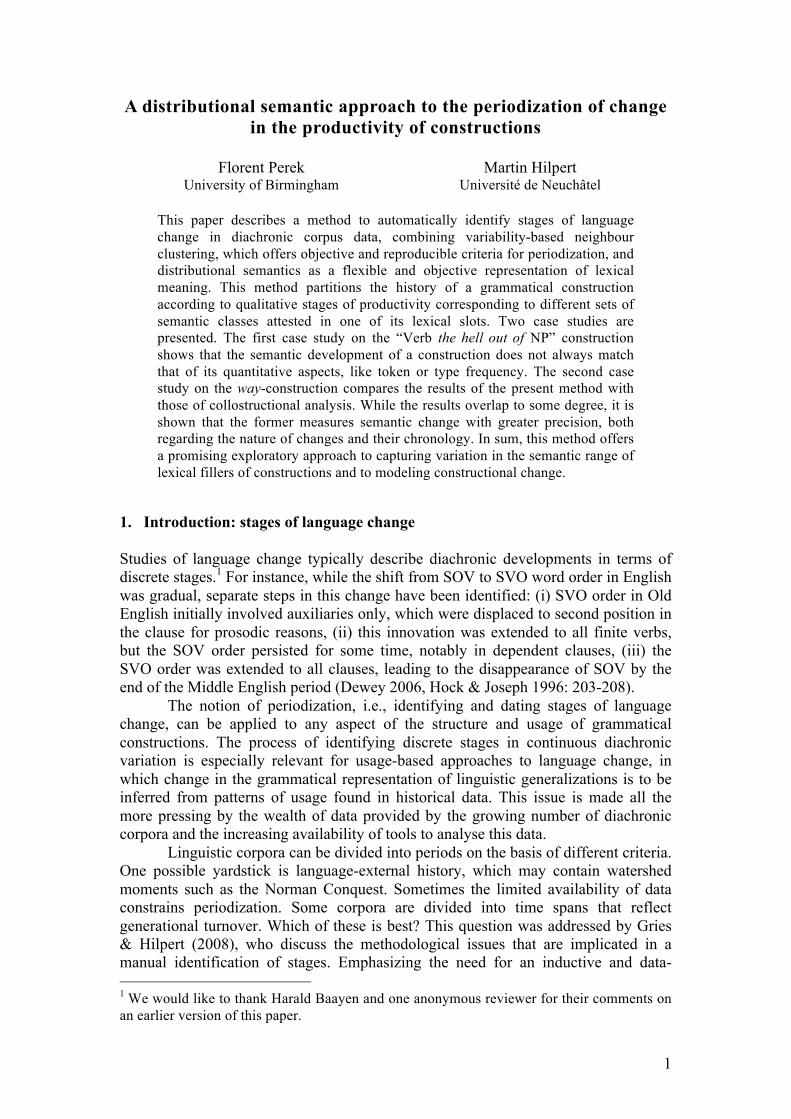
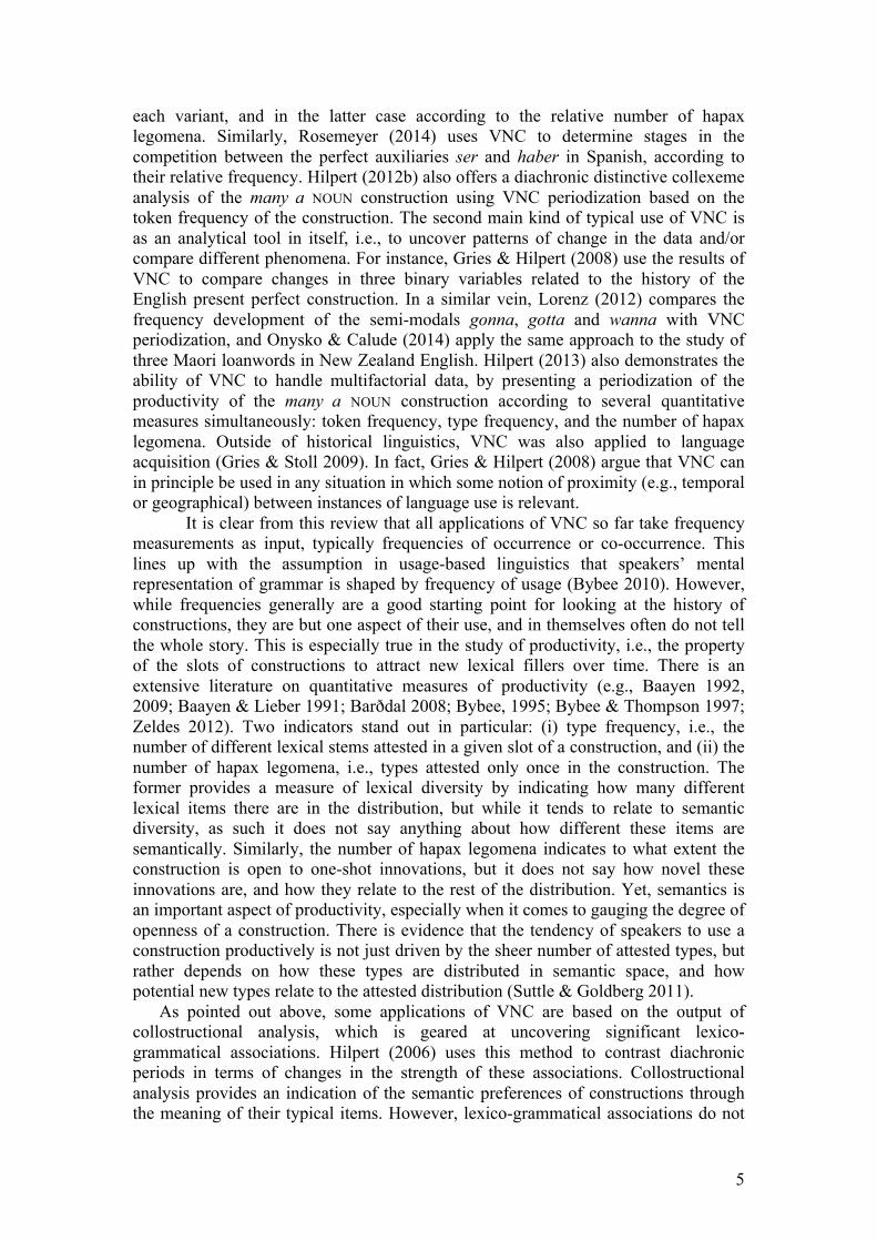
As an illustration, Figure 1 from Hilpert (2013: 30) shows the frequency development of two passive constructions, the get-passive (left) and the regular be-passive with a by-phrase (right), from the 1920s to the 2000s, using data from the TIME corpus. The aspect of the English language that is under scrutiny here is simply how common these two constructions are in usage. If one were to analyse these frequency trends in terms of discrete stages, it would be fairly easy to decide that the get-passive underwent an initial rise in frequency until the 1940s, then plateaued for a few decades, before soaring from the 1980s onwards. However, the picture is less

3

clear for the be-passive with by-phrase. For instance, the construction plummets in the first two decades, but should we consider the interruption of that fall in the 1940s and the subsequent resurgence as a separate phase of its own, or as a mere accident in what is essentially an overall decline of the construction over the period of interest?

Figure 1: Frequency variation of two passive constructions from 1920 to 2009 in the TIME corpus: the get-passive (left), e.g., He got fired, and the be-passive with a by-

phrase (right), e.g., He was fired by his boss (from Hilpert 2013: 30).

As pointed out by Gries & Hilpert (2008), manual periodization is potentially

subjective, especially when stages are not clear to discern: different groupings are possible for the same data, and without plain, objective, and reproducible criteria, different researchers might arrive at different partitions of the data. This, in turn, limits the possibility of comparing results between studies. Finally, while it is fairly easy to manually discern and describe stages of change in a single quantitative variable (notwithstanding the limitations indicated above), for instance by examining a time series plot, it becomes much more complex to infer stages when multiple variables are to be considered at the same time, for instance the token frequency and the type frequency of a construction.

To address these issues, Gries & Hilpert (2008) propose a new method for data-driven, bottom-up periodization, called variability-based neighbour clustering (VNC). VNC is a variant of an agglomerative hierarchical clustering algorithm, whereby items are recursively merged into higher-level groups according to some quantified criterion of similarity, to form a hierarchy of clusters. VNC submits time periods to hierarchical clustering according to how the linguistic phenomenon of interest varies across periods with regard to one or more pre-defined criteria. The crucial difference between VNC and regular hierarchical clustering is that only periods that are directly temporally adjacent are allowed to be merged. The chronological dimension of changes is thus preserved. The basis of VNC is data that is marked up for its time of production, typically years or decades. The algorithm starts by considering all pairs of adjacent periods (e.g., 1920s to 1930s, 1930s to 1940s, etc.), measuring the similarity between the members of each pair. The two periods found to be most similar are merged together to form a new higher-level period, whose properties are calculated by averaging over the properties of its constituent periods. The algorithm then proceeds to identifying the next two most similar periods, including the new higher-level period. The cycle is repeated until all

30 Data and methodology

1940 1960 1980 20000

5010

015

020

025

0

many a <NOUN>

Toke

ns p

er m

illio

n w

ords

1940 1960 1980 2000

01

23

45

That said, ...

1940 1960 1980 2000

5010

015

0

get−passive

Toke

ns p

er m

illio

n w

ords

1940 1960 1980 200070

080

090

010

0011

00

passive with by−phrase

Figure 2.1 Normalized frequency developments of four constructionsin TIME

the analysis of different constructional changes; and concrete examples onthe basis of corpus data will be offered to illustrate these methods.

2.2 Detecting and analyzing trends

One of the most basic issues in the analysis of constructional change isthe question whether a frequency shift that is observed in diachronic dataconstitutes a significant change or a mere chance fluctuation. Typically,diachronic corpus data are sparse, biased toward particular authors, genres, orvarieties, and either incomplete or unbalanced in its diachronic coverage. Allof these factors negatively affect the reliability of frequency measurements.A diachronic corpus that offers large amounts of regularly sampled data in asingle genre is the TIME corpus, which will be used in the following analyses.The four graphs in Figure 2.1 show the normalized frequency developments

4

periods have been merged into a single, superordinate cluster (see Gries & Hilpert 2008 for further details).

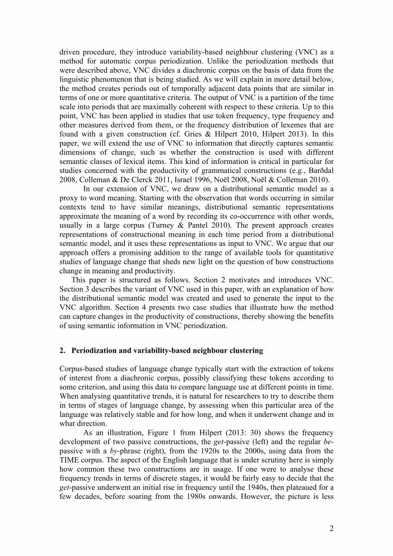
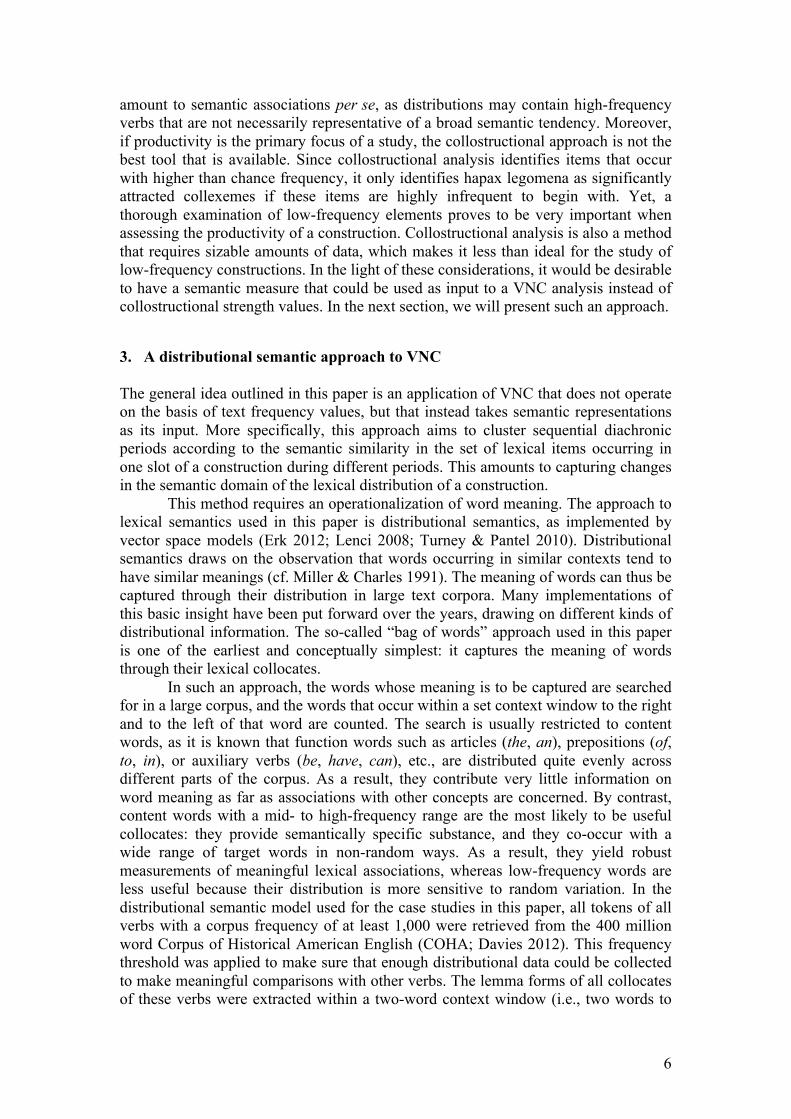
As a simple illustration of how VNC works, Figure 2 (taken from Hilpert 2013: 36) shows the results of the VNC algorithm applied to the get-passive frequency data presented in Figure 1. In this case, VNC operates with a single variable. The similarity between periods is calculated on the basis of their difference in frequency, and the frequency assigned to a cluster of periods is equal to the mean frequency of all of its constituent periods. The output of VNC is typically represented as a tree-like structure, or dendrogram, which is superimposed on the original frequency curve in Figure 2. Such a diagram captures the history of mergers produced by the algorithm. As can be seen in Figure 2, the decades that are first merged by the algorithm span from the 1940s to the 1980s: this corresponds to the plateau noted earlier. The periods before and after are merged later by the algorithm, and the higher position of these mergers in the dendrogram indicate that these periods are more distantly related, which also lines up with the earlier observation that they correspond to times of change.

Figure 2: VNC dendrogram of the get-passive frequency data (from Hilpert 2013: 36).

VNC has been applied to the study of various grammatical constructions in

diachrony. Two kinds of uses of VNC can be distinguished. The first kind involves using VNC to offer a data-driven and principled way to partition the data for further analysis. For instance, Gries & Hilpert (2008) cluster the distribution of the verbs occurring with the future auxiliary shall into different time periods in order to determine what partition of the data best reflects changes in lexico-grammatical associations. To do this, they turned raw co-occurrence frequencies into association scores along the lines of collostructional analysis (Gries & Stefanowitsch 2004, Hilpert 2006, Stefanowitsch & Gries 2003). Hilpert (2012a) applies the same method to the keep VERB-ing construction. In several studies, VNC is used to provide an initial periodization according to a key quantitative measure, and the individual stages that are inferred are then examined more closely. Hilpert (2013) uses this approach to analyze various types of constructional change, such as the possessive determiners mine/thyne vs. my/your, and the productivity of the derivational morpheme –ment. In the former case, the data is periodized according to the relative frequency of use of

36 Data and methodology

Time

Dis

tanc

e in

sum

med

sta

ndar

d de

viat

ions

1925 1935 1945 1955 1965 1975 1985 1995 2005

020

4060

8010

012

0

017

3350

6783

100

133

167

200

Toke

ns p

er m

illio

n w

ords

Figure 2.3 VNC results for the get-passive with overlaid frequencydevelopment

the 1970s and 1980s (62.4 and 64.9 respectively), which display a standarddeviation of 1.76. In the first iteration of the clustering process, these two aretherefore merged into a single data point. This is visualized in the secondpanel of Table 2.2, which serves as the basis for the second iteration of thealgorithm. This time, the 1940s and 1950s are the closest neighbors. Thethird panel of Table 2.2 shows this second merger. As the algorithm cyclesthrough the iterations, the time spans become larger until all nine periods aremerged into a single large structure. The visual result of a VNC applicationis a dendrogram. The graph shows which periods were merged; the heightsof the respective clusters indicate how different they are from one another.Figure 2.3 presents such a dendrogram for the get-passive.

The diagram shows several pieces of information at once: a dendrogram,the frequency development of the get-passive, and grey horizontal linesthat indicate the mean frequencies of four sequential clusters. To discussthe dendrogram first, it can be seen that indeed the 1970s and 1980s aremerged first, and that the height at which they are merged corresponds totheir standard deviation (1.76). The next two periods to be merged are the1940s and 1950s, which display the smallest standard deviation (2.75) in thesecond iteration of the algorithm. The first two standard deviations add upto 4.51, which is the height of the second cluster. Proceeding in this way,

5

each variant, and in the latter case according to the relative number of hapax legomena. Similarly, Rosemeyer (2014) uses VNC to determine stages in the competition between the perfect auxiliaries ser and haber in Spanish, according to their relative frequency. Hilpert (2012b) also offers a diachronic distinctive collexeme analysis of the many a NOUN construction using VNC periodization based on the token frequency of the construction. The second main kind of typical use of VNC is as an analytical tool in itself, i.e., to uncover patterns of change in the data and/or compare different phenomena. For instance, Gries & Hilpert (2008) use the results of VNC to compare changes in three binary variables related to the history of the English present perfect construction. In a similar vein, Lorenz (2012) compares the frequency development of the semi-modals gonna, gotta and wanna with VNC periodization, and Onysko & Calude (2014) apply the same approach to the study of three Maori loanwords in New Zealand English. Hilpert (2013) also demonstrates the ability of VNC to handle multifactorial data, by presenting a periodization of the productivity of the many a NOUN construction according to several quantitative measures simultaneously: token frequency, type frequency, and the number of hapax legomena. Outside of historical linguistics, VNC was also applied to language acquisition (Gries & Stoll 2009). In fact, Gries & Hilpert (2008) argue that VNC can in principle be used in any situation in which some notion of proximity (e.g., temporal or geographical) between instances of language use is relevant.

It is clear from this review that all applications of VNC so far take frequency measurements as input, typically frequencies of occurrence or co-occurrence. This lines up with the assumption in usage-based linguistics that speakers’ mental representation of grammar is shaped by frequency of usage (Bybee 2010). However, while frequencies generally are a good starting point for looking at the history of constructions, they are but one aspect of their use, and in themselves often do not tell the whole story. This is especially true in the study of productivity, i.e., the property of the slots of constructions to attract new lexical fillers over time. There is an extensive literature on quantitative measures of productivity (e.g., Baayen 1992, 2009; Baayen & Lieber 1991; Barðdal 2008; Bybee, 1995; Bybee & Thompson 1997; Zeldes 2012). Two indicators stand out in particular: (i) type frequency, i.e., the number of different lexical stems attested in a given slot of a construction, and (ii) the number of hapax legomena, i.e., types attested only once in the construction. The former provides a measure of lexical diversity by indicating how many different lexical items there are in the distribution, but while it tends to relate to semantic diversity, as such it does not say anything about how different these items are semantically. Similarly, the number of hapax legomena indicates to what extent the construction is open to one-shot innovations, but it does not say how novel these innovations are, and how they relate to the rest of the distribution. Yet, semantics is an important aspect of productivity, especially when it comes to gauging the degree of openness of a construction. There is evidence that the tendency of speakers to use a construction productively is not just driven by the sheer number of attested types, but rather depends on how these types are distributed in semantic space, and how potential new types relate to the attested distribution (Suttle & Goldberg 2011).

As pointed out above, some applications of VNC are based on the output of collostructional analysis, which is geared at uncovering significant lexico-grammatical associations. Hilpert (2006) uses this method to contrast diachronic periods in terms of changes in the strength of these associations. Collostructional analysis provides an indication of the semantic preferences of constructions through the meaning of their typical items. However, lexico-grammatical associations do not

6

amount to semantic associations per se, as distributions may contain high-frequency verbs that are not necessarily representative of a broad semantic tendency. Moreover, if productivity is the primary focus of a study, the collostructional approach is not the best tool that is available. Since collostructional analysis identifies items that occur with higher than chance frequency, it only identifies hapax legomena as significantly attracted collexemes if these items are highly infrequent to begin with. Yet, a thorough examination of low-frequency elements proves to be very important when assessing the productivity of a construction. Collostructional analysis is also a method that requires sizable amounts of data, which makes it less than ideal for the study of low-frequency constructions. In the light of these considerations, it would be desirable to have a semantic measure that could be used as input to a VNC analysis instead of collostructional strength values. In the next section, we will present such an approach.

3. A distributional semantic approach to VNC The general idea outlined in this paper is an application of VNC that does not operate on the basis of text frequency values, but that instead takes semantic representations as its input. More specifically, this approach aims to cluster sequential diachronic periods according to the semantic similarity in the set of lexical items occurring in one slot of a construction during different periods. This amounts to capturing changes in the semantic domain of the lexical distribution of a construction.

This method requires an operationalization of word meaning. The approach to lexical semantics used in this paper is distributional semantics, as implemented by vector space models (Erk 2012; Lenci 2008; Turney & Pantel 2010). Distributional semantics draws on the observation that words occurring in similar contexts tend to have similar meanings (cf. Miller & Charles 1991). The meaning of words can thus be captured through their distribution in large text corpora. Many implementations of this basic insight have been put forward over the years, drawing on different kinds of distributional information. The so-called “bag of words” approach used in this paper is one of the earliest and conceptually simplest: it captures the meaning of words through their lexical collocates.

In such an approach, the words whose meaning is to be captured are searched for in a large corpus, and the words that occur within a set context window to the right and to the left of that word are counted. The search is usually restricted to content words, as it is known that function words such as articles (the, an), prepositions (of, to, in), or auxiliary verbs (be, have, can), etc., are distributed quite evenly across different parts of the corpus. As a result, they contribute very little information on word meaning as far as associations with other concepts are concerned. By contrast, content words with a mid- to high-frequency range are the most likely to be useful collocates: they provide semantically specific substance, and they co-occur with a wide range of target words in non-random ways. As a result, they yield robust measurements of meaningful lexical associations, whereas low-frequency words are less useful because their distribution is more sensitive to random variation. In the distributional semantic model used for the case studies in this paper, all tokens of all verbs with a corpus frequency of at least 1,000 were retrieved from the 400 million word Corpus of Historical American English (COHA; Davies 2012). This frequency threshold was applied to make sure that enough distributional data could be collected to make meaningful comparisons with other verbs. The lemma forms of all collocates of these verbs were extracted within a two-word context window (i.e., two words to

7

the right and two words to the left). The collocate search was restricted to the 10,000 most frequent nouns, verbs, adjectives and adverbs, and it was sensitive to the part-of-speech tags found in the corpus; in other words, words with the same lemma but from a different part-of-speech (e.g. question as a noun and as a verb) were counted as distinct collocates.

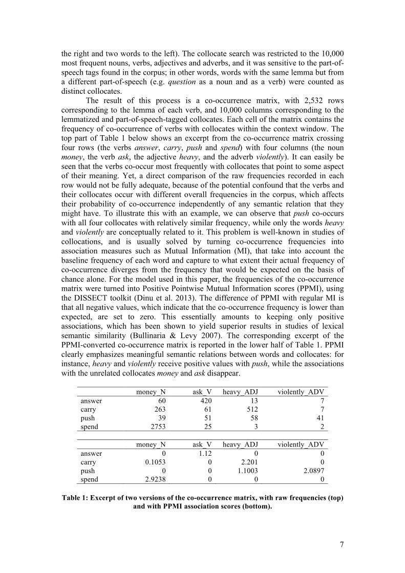
The result of this process is a co-occurrence matrix, with 2,532 rows corresponding to the lemma of each verb, and 10,000 columns corresponding to the lemmatized and part-of-speech-tagged collocates. Each cell of the matrix contains the frequency of co-occurrence of verbs with collocates within the context window. The top part of Table 1 below shows an excerpt from the co-occurrence matrix crossing four rows (the verbs answer, carry, push and spend) with four columns (the noun money, the verb ask, the adjective heavy, and the adverb violently). It can easily be seen that the verbs co-occur most frequently with collocates that point to some aspect of their meaning. Yet, a direct comparison of the raw frequencies recorded in each row would not be fully adequate, because of the potential confound that the verbs and their collocates occur with different overall frequencies in the corpus, which affects their probability of co-occurrence independently of any semantic relation that they might have. To illustrate this with an example, we can observe that push co-occurs with all four collocates with relatively similar frequency, while only the words heavy and violently are conceptually related to it. This problem is well-known in studies of collocations, and is usually solved by turning co-occurrence frequencies into association measures such as Mutual Information (MI), that take into account the baseline frequency of each word and capture to what extent their actual frequency of co-occurrence diverges from the frequency that would be expected on the basis of chance alone. For the model used in this paper, the frequencies of the co-occurrence matrix were turned into Positive Pointwise Mutual Information scores (PPMI), using the DISSECT toolkit (Dinu et al. 2013). The difference of PPMI with regular MI is that all negative values, which indicate that the co-occurrence frequency is lower than expected, are set to zero. This essentially amounts to keeping only positive associations, which has been shown to yield superior results in studies of lexical semantic similarity (Bullinaria & Levy 2007). The corresponding excerpt of the PPMI-converted co-occurrence matrix is reported in the lower half of Table 1. PPMI clearly emphasizes meaningful semantic relations between words and collocates: for instance, heavy and violently receive positive values with push, while the associations with the unrelated collocates money and ask disappear.

money_N ask_V heavy_ADJ violently_ADV answer 60 420 13 7 carry 263 61 512 7 push 39 51 58 41 spend 2753 25 3 2 money_N ask_V heavy_ADJ violently_ADV answer 0 1.12 0 0 carry 0.1053 0 2.201 0 push 0 0 1.1003 2.0897 spend 2.9238 0 0 0

Table 1: Excerpt of two versions of the co-occurrence matrix, with raw frequencies (top)

and with PPMI association scores (bottom).

8

To the extent that collocates capture aspects of word meaning, the process

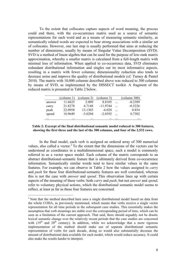
could end there, with the co-occurrence matrix used as a source of semantic representations for each word and as a means of measuring semantic similarity, as semantically related words are expected to bear strong associations with a similar set of collocates. However, one last step is usually performed that aims at reducing the number of dimensions, usually by means of Singular Value Decomposition (SVD). SVD is a method of linear algebra that can be used for the purpose of low-rank matrix approximation, whereby a smaller matrix is calculated from a full-length matrix with minimal loss of information. When applied to co-occurrence data, SVD eliminates redundant distributional information and singles out its most informative aspects, resulting in a matrix with fewer columns; dimensionality reduction also tends to decrease noise and improve the quality of distributional models (cf. Turney & Pantel 2010). The matrix with 10,000 columns described above was reduced to 300 columns by means of SVD, as implemented by the DISSECT toolkit. A fragment of the reduced matrix is presented in Table 2 below.

(column 1) (column 2) (column 3) (column 300) answer 11.6625 2.009 8.8105 ... -0.2389 carry 21.8278 4.7148 -11.9744 ... -0.5226 push 22.0958 13.1303 -6.028 ... 0.854 spend 10.9649 -3.0204 -2.0392 ... 0.7302 ... ... ... ... ... ...

Table 2: Excerpt of the final distributional semantic model reduced to 300 features, showing the first three and the last of the 300 columns, and four of the 2,532 rows.

In the final model, each verb is assigned an ordered array of 300 numerical

values, also called a vector.2 To the extent that the dimensions of the vectors can be understood as coordinates in a multidimensional space, such a model is commonly referred to as a vector space model. Each column of the matrix corresponds to an abstract distributional-semantic feature that is ultimately derived from co-occurrence information. Semantically similar words tend to have similar values in the same features. For example, we can observe in Table 2 how the values assigned to carry and push for these four distributional-semantic features are well correlated, whereas this is not the case with answer and spend. This observation lines up with certain aspects of the meaning of these verbs: both carry and push, but not answer and spend, refer to voluntary physical actions, which the distributional semantic model seems to reflect, at least as far as these four features are concerned. 2 Note that the method described here uses a single distributional model based on data from the whole COHA, as previously mentioned, which means that verbs receive a single vector representation for all time periods in the subsequent case studies. This essentially makes the assumption that verb meanings are stable over the corresponding period of time, which can be seen as a limitation of the current approach. That said, there should arguably not be drastic lexical semantic change over the relatively recent periods that the case studies are concerned with (19th and 20th century). In addition, while we acknowledge that a more rigorous implementation of the method should make use of separate distributional semantic representation of verbs for each decade, doing so would also substantially decrease the amount of distributional data available for each model, which would reduce accuracy. It could also make the results harder to interpret.

9

Distributional semantics in general, and their vector space model implementation in particular, offer a number of benefits for the present approach. First, it is entirely data-driven, which means that no manual intervention is needed (such as semantic annotations), and also makes it arguably more objective than introspective data, in that semantic information is derived from how words are actually used in thousands of contexts by many different speakers rather than from the semantic intuitions of a limited number of informants. Second, the method does not put any limit on the number of lexical items that may be considered, contrary to some other approaches such as norming studies of semantic similarity (e.g. Bybee & Eddington 2006). Third, while the cognitive status of distributional semantics is still debated (cf. Glenberg & Robertson 2000), there is ample evidence that current implementations of the approach produce robust semantic representations that capture aspects of human semantic knowledge. Distributional models have been reported to correlate well with human performance on a number of tasks (e.g., Landauer et al. 1998, Lund et al. 1995), and there is some evidence suggesting that human language learners do acquire a fair share of lexical semantic knowledge by tracking co-occurrence statistics (Andrews et al. 2014, Dąbrowska 2009).

This is not to say that distributional semantics is without limitations. As pointed out by one anonymous reviewer, distributional approaches to meaning typically ignore polysemy and homonymy, in that distributional information is assigned to word forms, and thus each word form is associated with a single semantic representation, regardless of how diverse the different uses of this word are. While this is not an issue for monosemous words and highly related polysemes, it means that distributional-semantic data for truly homonymous words should be taken with a pinch of salt, especially if none of the senses of the words is strikingly more common than the others. Distributional approaches also disregard the fact that not all collocates of a word should be given equal weight in measuring semantic similarity with other words (consider for instance, collocates involved in a compound vs. a syntactic dependency vs. the same clause but in a different unrelated constituent). Some more recent variants of the distributional approach attempt to address some of these problems. While the limitations of distributional approaches should be kept in mind, they do not represent fundamental problems. Any of these shortcomings are largely outweighed by the potential advantages that the approach offers.

Finally, and very importantly for the present purpose, distributional semantic models allow for precise quantification of meaning and semantic similarity, and the representations of meaning that they provide possess mathematical properties that are interesting for the application to VNC. As pointed out earlier, semantic similarity between words is reflected by similarity in their semantic vectors, which can be quantified by standard measures of distance and correlation. The cosine distance is by far the most frequently used option for that purpose. It has the property of normalizing the magnitude of distributional-semantic associations by capturing a correlation between vectors (as opposed to sheer closeness). The cosine function is sensitive to whether two vectors point in the same direction in the multidimensional semantic space, but it is unaffected by vector length. Also, using vector algebra, vector representations of meaning can be easily combined in useful ways for the present purpose.

Returning to our initial goal, how can such a distributional semantic model be harnessed for use with VNC, for the purpose of capturing stages of semantic change in the lexical distribution of a construction? This first requires building representations of the semantic range of a construction at different points in time. One

10

possible way to do this using distributional semantics, which will be tested in this paper, involves the following steps:

1. For each period, extract the semantic vector of each lexical item (here, verbs) attested in the construction.

2. Sum all the word vectors. 3. Divide the sum vector by the number of items in the distribution; the result is

the period vector. Summing vectors means adding all of their values together in each dimension;

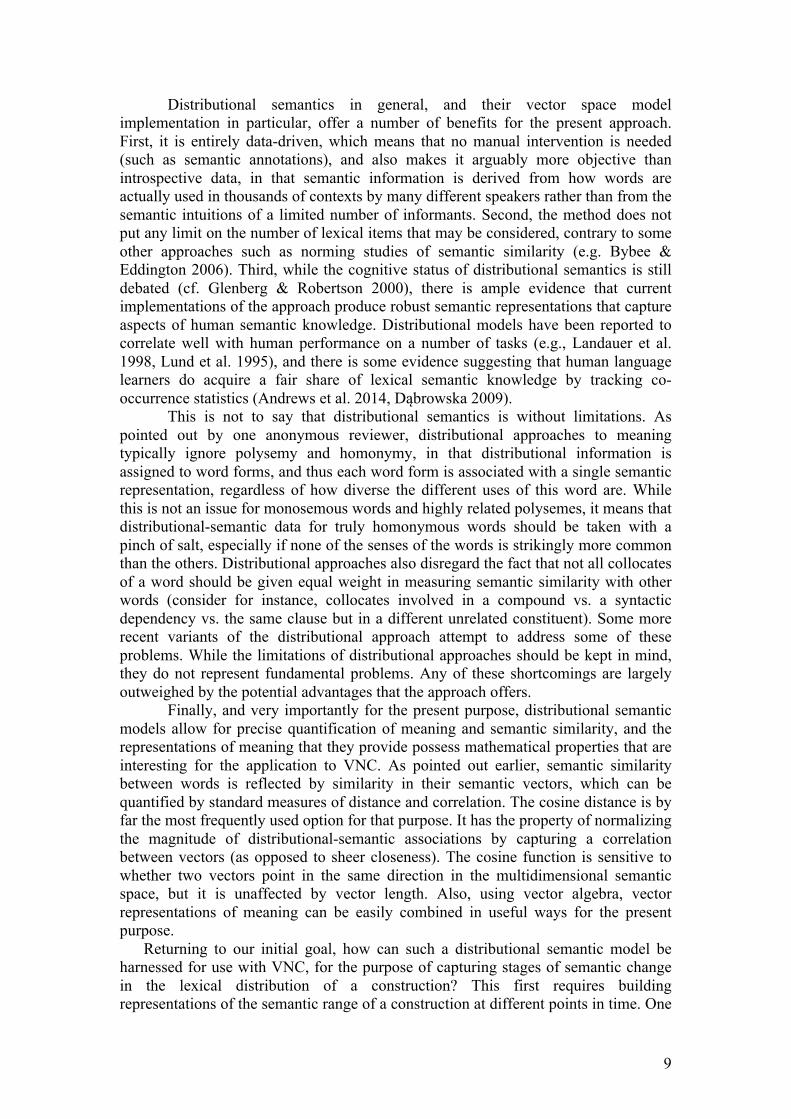
only vectors of the same length can be summed (which is the case here), resulting in a vector of that length. To take a fictitious example, let us imagine a construction that is attested in a given period with the four verbs discussed above (and only these four): answer, carry, push, and spend. The vector representations of these verbs in the distributional semantic model are repeated in Table 3 below, line by line. To calculate the period vector, the figures in each column are first summed (see fifth line). The sum in each column is then divided by the total number of verbs, here four, as presented in the last line of Table 3.

(column 1) (column 2) (column 3) (column 300) answer 11.6625 2.009 8.8105 ... -0.2389 carry 21.8278 4.7148 -11.9744 ... -0.5226 push 22.0958 13.1303 -6.028 ... 0.854 spend 10.9649 -3.0204 -2.0392 ... 0.7302 Sum 66.5509 16.8337 -11.2311 ... 0.8226

Divided by 4 (period vector) 16.6377 4.2084 -2.8078 ... 0.2056

Table 3: Calculation of the period vector for the fictitious example of a construction

occurring in this period with the four verbs answer, carry, push, and spend.

As mentioned earlier, the dimensions of semantic vectors correspond to distributional-semantic features that relate to aspects of word meaning. Words that receive high values in the same features tend to share parts of their semantics. Hence, features of the period vector reflect semantic properties of the lexical items attested in the period; the period vector literally represents the “semantic average” of the distribution, since each of its features equals the mean value of that feature across all words in the distribution. If words sharing certain features join the distribution at a given period, this will be reflected in the period vector by an adjustment in the values of these features. In effect, the period vector acts as a global semantic representation of the types attested in a construction.

Once all period vectors have been calculated, the VNC algorithm can be run on these vectors, in very much the same way that it was applied to lexical distributions (which are essentially vectors as well; cf. Gries & Hilpert 2008). The resulting dendrogram traces the semantic history of the construction with respect to its lexical distribution, with early mergers corresponding to periods of semantic stability, and late mergers indicating semantic shifts. In the implementation used in this paper, similarity between period vectors is calculated with the cosine measure, as is standard practice in distributional semantics, and the semantic representation of a period cluster is calculated from the average of the semantic representations of all its constituent periods. In the next section, the method just described is illustrated by two case studies examining the productivity of two grammatical constructions.

11

4. Case studies This section presents two case studies that illustrate the distribution semantic approach to VNC described above. We draw on diachronic data in order to analyze two grammatical constructions: the so-called hell-construction, e.g., You scared the hell out of me (Hoeksema & Napoli 2008, Perek 2016a), and the way-construction, e.g., They pushed their way through the crowd (Goldberg 1995, Israel 1996). In both cases, the distribution of verbs occurring in the construction is used to build distributional semantic representations for each time period, and these representations are submitted to the VNC algorithm. In the first case, the semantic development indicated by the distributional semantic VNC analysis turns out to be quite different from the stages inferred on the basis of quantitative measures of productivity, which leads us to question the idea that quantitative and qualitative information about the productivity of constructions have to go hand in hand. In the second case, the results of the distributional semantic approach to VNC is compared to those of its most similar equivalent in the current literature, diachronic distinctive collexeme analysis (Hilpert 2006). It is shown that while the two do overlap, they also differ on some aspects of periodization, and on the amount and kind of semantic information that they reveal, which owes much to the different perspectives that they take.

4.1. The hell-construction The first case study is concerned with a construction consisting of a verb followed by the sequence the hell out of and a noun phrase, as exemplified by (1) and (2) below (from COHA).

(1) Anatoly is a terrible driver and this scares the hell out of Vladimir.

(2) They beat the hell out of me to remember them.

In such sentences, since the hell is not referential and since the overall interpretation cannot be straightforwardly derived from the meaning of the parts, the entire pattern “V the hell out of NP” is best analysed as a direct pairing of form and meaning, which Perek (2016a) has termed the hell-construction (see also Hoeksema & Napoli 2008). The general semantic contribution of the construction is, broadly speaking, to intensify the meaning of the verb. It is a relatively recent construction in the history of English, since the first instance attested in the COHA only date back to the 1930s. Instances of the construction with scare and beat are intuitively perceived as typical, and indeed these two verbs turn out to be particularly frequent in the construction; yet, a wide range of different verbs are attested, as exemplified by sentences (3) to (5) below from the COHA.

(3) Leave it to Patrick to take a simple issue and complicate the hell out of it.

(4) Do you know I want the hell out of you? (5) We bombed the hell out of those cities.

All instances of a verb followed by the words the hell out of were extracted

from the COHA and manually filtered to keep only the instances of the construction, leaving 362 tokens distributed over 105 verb types. This makes it a very infrequent construction relative to the 200 million words totalled by the eight last decades of the

12

corpus in which the construction is attested (from 1930 to 2009). In each decade, most types are very infrequent, which makes collostructional analysis a problematic choice for studying the construction. Significance testing on the basis of low frequencies is of course possible if tests such as the Fisher Exact test are used, but it is clear that the results will be highly sensitive to differences in sampling: Two different corpora might yield substantially different results.

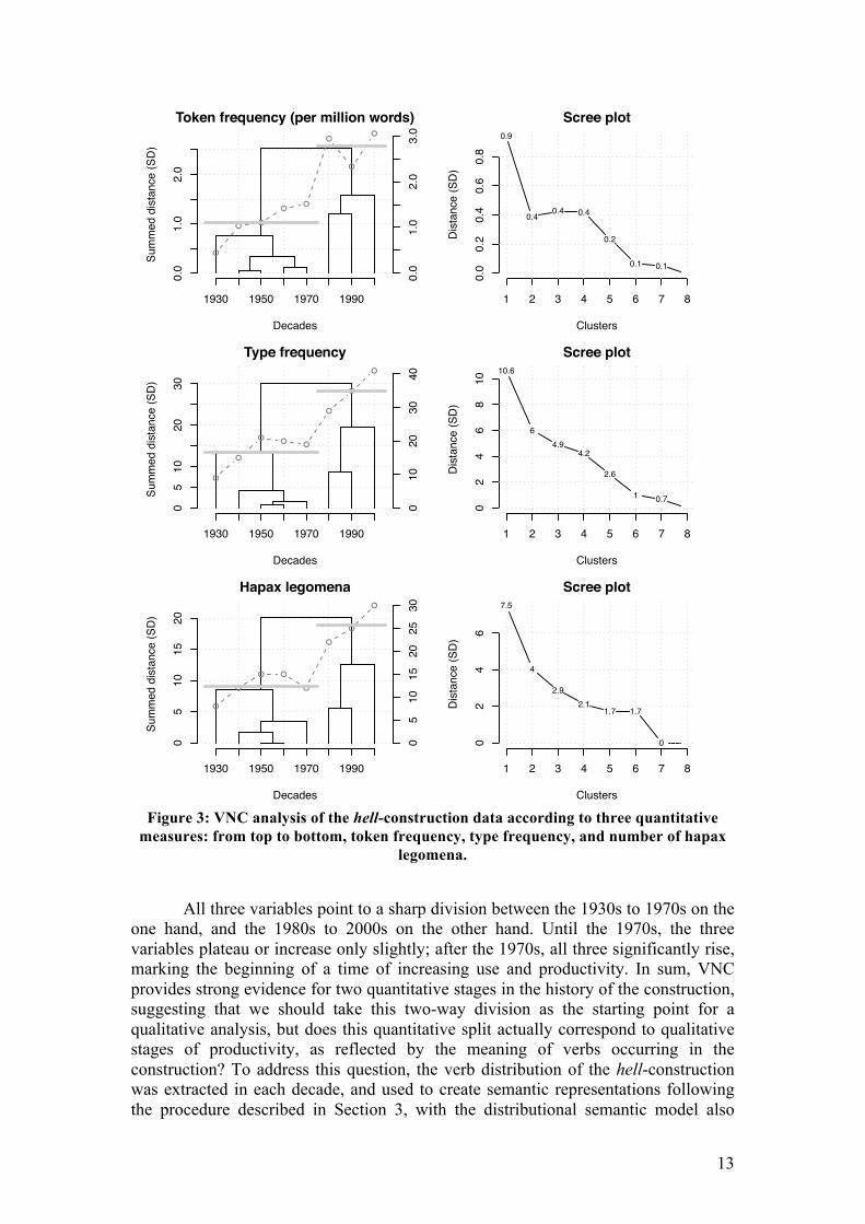
In keeping with one of the typical uses of VNC in diachronic studies of constructions, let us first evaluate whether VNC allows us to discern stages of usage in the history of the hell-construction according to quantitative measures. Figure 3 below presents the dendrograms of three VNC analyses of the data, according to, from top to bottom, token frequency, type frequency, and the number of hapax legomena. The plot line of the relevant variable (with the corresponding scale on the right) is superimposed to the VNC dendrogram in each case. ‘Scree’ plots are presented next to each dendrogram to help decide on the appropriate number of clusters; these plots indicate how much dissimilarity between clusters (in the y-axis) is involved in the lowest-level merger every time a new cluster is added (in the x-axis). The appropriate number of clusters is reached when adding a cluster would result in a markedly less sharp decrease in dissimilarity, meaning that the merger involves items that are relatively similar to each other compared to the clusters identified so far. This breaking point or “elbow” can be visualized as a bend in the plot’s curve. In all three cases, a two-cluster solution appears to be preferable. The corresponding two clusters are marked in each dendrogram by grey vertical lines spanning over the decades contained by the cluster, and vertically positioned at the mean value of these decades.

13

Figure 3: VNC analysis of the hell-construction data according to three quantitative

measures: from top to bottom, token frequency, type frequency, and number of hapax legomena.

All three variables point to a sharp division between the 1930s to 1970s on the

one hand, and the 1980s to 2000s on the other hand. Until the 1970s, the three variables plateau or increase only slightly; after the 1970s, all three significantly rise, marking the beginning of a time of increasing use and productivity. In sum, VNC provides strong evidence for two quantitative stages in the history of the construction, suggesting that we should take this two-way division as the starting point for a qualitative analysis, but does this quantitative split actually correspond to qualitative stages of productivity, as reflected by the meaning of verbs occurring in the construction? To address this question, the verb distribution of the hell-construction was extracted in each decade, and used to create semantic representations following the procedure described in Section 3, with the distributional semantic model also

Token frequency (per million words)

Decades

Sum

med

dis

tanc

e (S

D)

1930 1950 1970 1990

0.0

1.0

2.0

●

● ●

●●

●

●

●

0.0

1.0

2.0

3.0

Scree plot

Clusters

Dis

tanc

e (S

D)

1 2 3 4 5 6 7 8

0.0

0.2

0.4

0.6

0.8

0.9

0.40.4 0.4

0.2

0.1 0.1

Type frequency

Decades

Sum

med

dis

tanc

e (S

D)

1930 1950 1970 1990

05

1020

30

●

●

●●

●

●

●

●

010

2030

40

Scree plot

Clusters

Dis

tanc

e (S

D)

1 2 3 4 5 6 7 8

02

46

810

10.6

64.9

4.2

2.6

1 0.7

Hapax legomena

Decades

Sum

med

dis

tanc

e (S

D)

1930 1950 1970 1990

05

1015

20

●

●

● ●

●

●

●

●

05

1015

2025

30

Scree plot

Clusters

Dis

tanc

e (S

D)

1 2 3 4 5 6 7 8

02

46

7.5

4

2.92.1

1.7 1.7

0

14

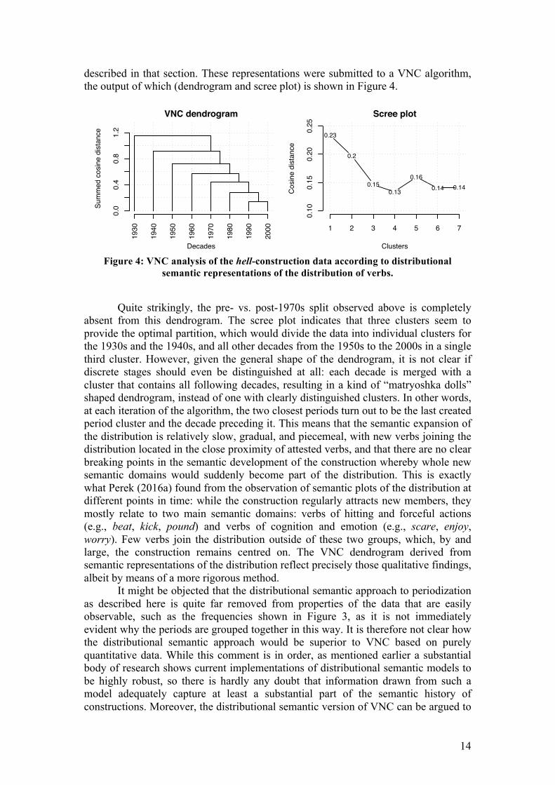
described in that section. These representations were submitted to a VNC algorithm, the output of which (dendrogram and scree plot) is shown in Figure 4.

Figure 4: VNC analysis of the hell-construction data according to distributional

semantic representations of the distribution of verbs.

Quite strikingly, the pre- vs. post-1970s split observed above is completely

absent from this dendrogram. The scree plot indicates that three clusters seem to provide the optimal partition, which would divide the data into individual clusters for the 1930s and the 1940s, and all other decades from the 1950s to the 2000s in a single third cluster. However, given the general shape of the dendrogram, it is not clear if discrete stages should even be distinguished at all: each decade is merged with a cluster that contains all following decades, resulting in a kind of “matryoshka dolls” shaped dendrogram, instead of one with clearly distinguished clusters. In other words, at each iteration of the algorithm, the two closest periods turn out to be the last created period cluster and the decade preceding it. This means that the semantic expansion of the distribution is relatively slow, gradual, and piecemeal, with new verbs joining the distribution located in the close proximity of attested verbs, and that there are no clear breaking points in the semantic development of the construction whereby whole new semantic domains would suddenly become part of the distribution. This is exactly what Perek (2016a) found from the observation of semantic plots of the distribution at different points in time: while the construction regularly attracts new members, they mostly relate to two main semantic domains: verbs of hitting and forceful actions (e.g., beat, kick, pound) and verbs of cognition and emotion (e.g., scare, enjoy, worry). Few verbs join the distribution outside of these two groups, which, by and large, the construction remains centred on. The VNC dendrogram derived from semantic representations of the distribution reflect precisely those qualitative findings, albeit by means of a more rigorous method.

It might be objected that the distributional semantic approach to periodization as described here is quite far removed from properties of the data that are easily observable, such as the frequencies shown in Figure 3, as it is not immediately evident why the periods are grouped together in this way. It is therefore not clear how the distributional semantic approach would be superior to VNC based on purely quantitative data. While this comment is in order, as mentioned earlier a substantial body of research shows current implementations of distributional semantic models to be highly robust, so there is hardly any doubt that information drawn from such a model adequately capture at least a substantial part of the semantic history of constructions. Moreover, the distributional semantic version of VNC can be argued to

VNC dendrogram

Decades

Sum

med

cos

ine

dist

ance

1930

1940

1950

1960

1970

1980

1990

2000

0.0

0.4

0.8

1.2

Scree plot

Clusters

Cos

ine

dist

ance

1 2 3 4 5 6 7

0.10

0.15

0.20

0.25

0.23

0.2

0.150.13

0.160.14 0.14

15

be less sensitive to statistical artefacts by design than one based on quantitative information alone, since by capturing the semantics of types it has the ability to “smooth over” potential outlier types.

At any rate, the important point that can be made from this case study is not necessarily that one type of VNC periodization is superior to the other, but that they do not coincide. Specifically, quantitative measures suggest a shift that is not qualitatively reflected in the distribution of the construction. The dissonance between the quantitative and qualitative history of the construction, as inferred by VNC in the former case on the basis of several quantitative measures, and in the latter case on the basis of distributional semantic vectors of the verbs occurring in it, should not be entirely surprising, as the two uses of VNC really show different kinds of information. That said, while this finding does not directly question the practice of using VNC to partition the data according to quantitative measures as a starting point for studying language change, it does suggest that this practice is not always appropriate in the context of the study of productivity in diachrony.

4.2. The way-construction

4.2.1. Distributional-semantic VNC analysis of the way-construction The way-construction is a textbook example of a grammatical form-meaning pairing along the lines of construction grammar (Goldberg 1995). It consists of a verb followed by a possessive determiner co-referential with the subject of the verb (e.g., my, her, their, etc.), the noun way, and a prepositional phrase expressing a direction, as exemplified by the following sentences from COHA:

(6) The outlaw chief pushed his way through the dense mob at the door.

(7) He kicked his way through a drift of snow. (8) You can usually talk or bluff your way out of trouble.

(9) Nicklaus slowly edged his way into a lead that Jacobs could not close. (10) I got out of the car and smoked my way toward the restaurant.

Sentences (6) to (8) instantiate the most common use of the construction, in

which the verb refers to some action performed by the subject referent that enables or causes their motion along the specified path. This use, which Traugott & Trousdale (2013) call the path-creation sense, is the one that this case study will focus on, to the exclusion of the less common uses of the construction where the verb refers to the manner in which the agent moves, as shown in example (9), or to some incidental action performed during motion but not directly related to it, as shown in example (10).

All instances of the way-construction were extracted from the COHA, manually filtered and annotated for the sense of the construction (path-creation, manner, incidental action). Only tokens of the path-creation sense occurring from the 1830s; although the corpus also covers the 1810s and 1820s, these decades were excluded because they are smaller and have a different genre balance. This left 15,446 tokens distributed over 958 verb types. As previously, distributional semantic representations were derived for each decade from the distribution of verbs, and these semantic vectors were submitted to VNC in order to determine stages of semantic

16

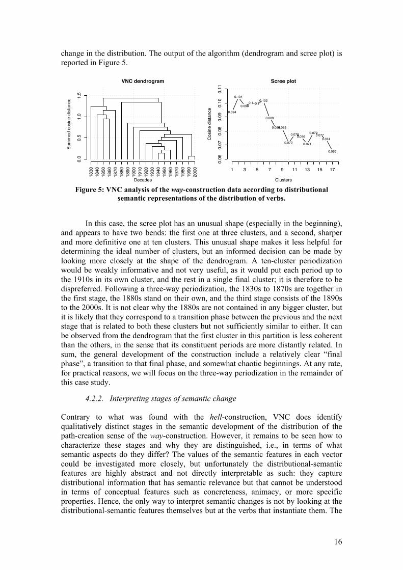
change in the distribution. The output of the algorithm (dendrogram and scree plot) is reported in Figure 5.

Figure 5: VNC analysis of the way-construction data according to distributional

semantic representations of the distribution of verbs.

In this case, the scree plot has an unusual shape (especially in the beginning),

and appears to have two bends: the first one at three clusters, and a second, sharper and more definitive one at ten clusters. This unusual shape makes it less helpful for determining the ideal number of clusters, but an informed decision can be made by looking more closely at the shape of the dendrogram. A ten-cluster periodization would be weakly informative and not very useful, as it would put each period up to the 1910s in its own cluster, and the rest in a single final cluster; it is therefore to be dispreferred. Following a three-way periodization, the 1830s to 1870s are together in the first stage, the 1880s stand on their own, and the third stage consists of the 1890s to the 2000s. It is not clear why the 1880s are not contained in any bigger cluster, but it is likely that they correspond to a transition phase between the previous and the next stage that is related to both these clusters but not sufficiently similar to either. It can be observed from the dendrogram that the first cluster in this partition is less coherent than the others, in the sense that its constituent periods are more distantly related. In sum, the general development of the construction include a relatively clear “final phase”, a transition to that final phase, and somewhat chaotic beginnings. At any rate, for practical reasons, we will focus on the three-way periodization in the remainder of this case study.

4.2.2. Interpreting stages of semantic change Contrary to what was found with the hell-construction, VNC does identify qualitatively distinct stages in the semantic development of the distribution of the path-creation sense of the way-construction. However, it remains to be seen how to characterize these stages and why they are distinguished, i.e., in terms of what semantic aspects do they differ? The values of the semantic features in each vector could be investigated more closely, but unfortunately the distributional-semantic features are highly abstract and not directly interpretable as such: they capture distributional information that has semantic relevance but that cannot be understood in terms of conceptual features such as concreteness, animacy, or more specific properties. Hence, the only way to interpret semantic changes is not by looking at the distributional-semantic features themselves but at the verbs that instantiate them. The

VNC dendrogram

Decades

Sum

med

cos

ine

dist

ance

1830

1840

1850

1860

1870

1880

1890

1900

1910

1920

1930

1940

1950

1960

1970

1980

1990

2000

0.0

0.5

1.0

1.5

Scree plot

Clusters

Cos

ine

dist

ance

1 3 5 7 9 11 13 15 17

0.06

0.07

0.08

0.09

0.10

0.11

0.094

0.104

0.0980.1 0.1

0.102

0.089

0.0830.083

0.072

0.0780.076

0.071

0.0790.0770.074

0.065

17

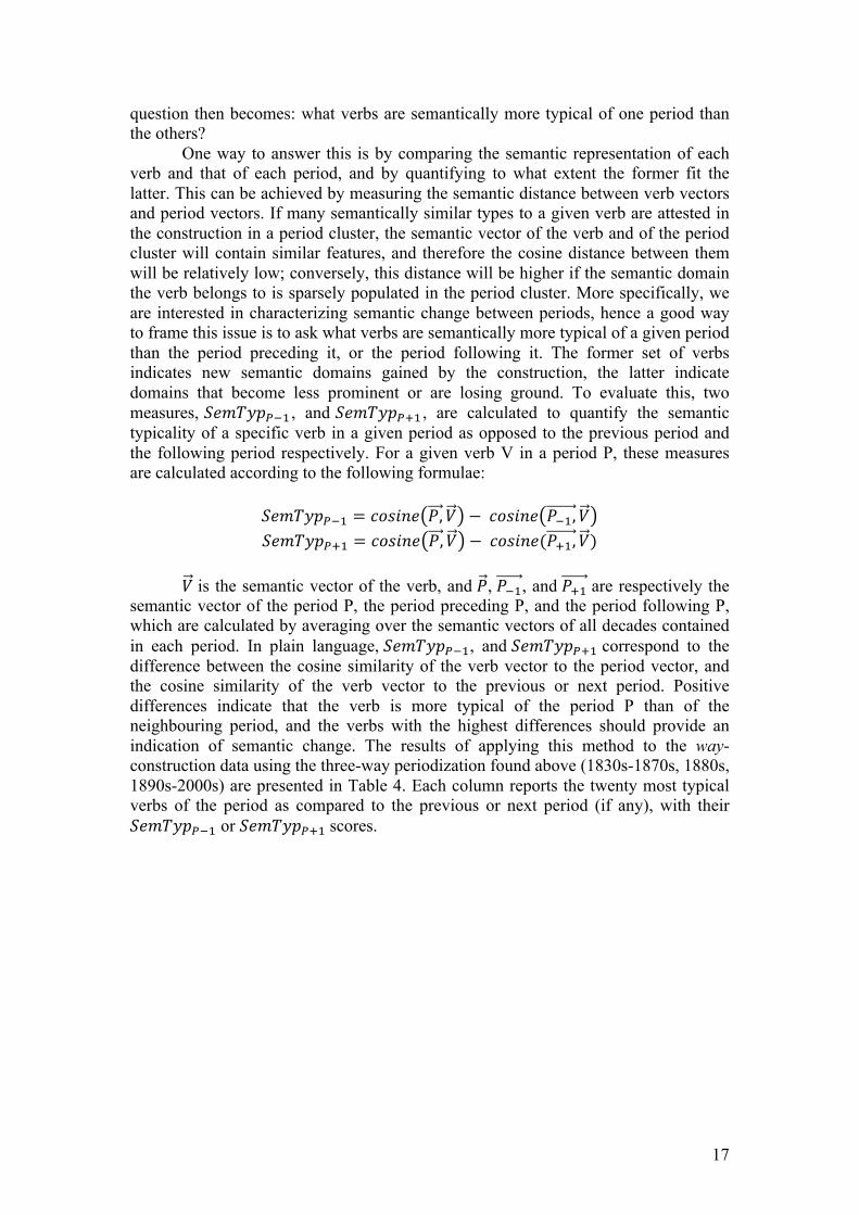
question then becomes: what verbs are semantically more typical of one period than the others?

One way to answer this is by comparing the semantic representation of each verb and that of each period, and by quantifying to what extent the former fit the latter. This can be achieved by measuring the semantic distance between verb vectors and period vectors. If many semantically similar types to a given verb are attested in the construction in a period cluster, the semantic vector of the verb and of the period cluster will contain similar features, and therefore the cosine distance between them will be relatively low; conversely, this distance will be higher if the semantic domain the verb belongs to is sparsely populated in the period cluster. More specifically, we are interested in characterizing semantic change between periods, hence a good way to frame this issue is to ask what verbs are semantically more typical of a given period than the period preceding it, or the period following it. The former set of verbs indicates new semantic domains gained by the construction, the latter indicate domains that become less prominent or are losing ground. To evaluate this, two measures, 𝑆𝑒𝑚𝑇𝑦𝑝!!! , and 𝑆𝑒𝑚𝑇𝑦𝑝!!! , are calculated to quantify the semantic typicality of a specific verb in a given period as opposed to the previous period and the following period respectively. For a given verb V in a period P, these measures are calculated according to the following formulae:

𝑆𝑒𝑚𝑇𝑦𝑝!!! = 𝑐𝑜𝑠𝑖𝑛𝑒 𝑃,𝑉 − 𝑐𝑜𝑠𝑖𝑛𝑒 𝑃!!,𝑉 𝑆𝑒𝑚𝑇𝑦𝑝!!! = 𝑐𝑜𝑠𝑖𝑛𝑒 𝑃,𝑉 − 𝑐𝑜𝑠𝑖𝑛𝑒(𝑃!!,𝑉)

𝑉 is the semantic vector of the verb, and 𝑃, 𝑃!!, and 𝑃!! are respectively the semantic vector of the period P, the period preceding P, and the period following P, which are calculated by averaging over the semantic vectors of all decades contained in each period. In plain language, 𝑆𝑒𝑚𝑇𝑦𝑝!!!, and 𝑆𝑒𝑚𝑇𝑦𝑝!!! correspond to the difference between the cosine similarity of the verb vector to the period vector, and the cosine similarity of the verb vector to the previous or next period. Positive differences indicate that the verb is more typical of the period P than of the neighbouring period, and the verbs with the highest differences should provide an indication of semantic change. The results of applying this method to the way-construction data using the three-way periodization found above (1830s-1870s, 1880s, 1890s-2000s) are presented in Table 4. Each column reports the twenty most typical verbs of the period as compared to the previous or next period (if any), with their 𝑆𝑒𝑚𝑇𝑦𝑝!!! or 𝑆𝑒𝑚𝑇𝑦𝑝!!! scores.

18

P = 1830s – 1870s P = 1880s P = 1890s – 2000s Verbs more typical of P

than P + 1 Verbs more typical of

P than P - 1 Verbs more typical of P

than P + 1 Verbs more typical of

P than P - 1 Verb SemTypP+1 Verb SemTypP-1 Verb SemTypP+1 Verb SemTypP-1 hew 0.0689 guess 0.0553 bore 0.0494 punch 0.0625

shape 0.0657 buy 0.0521 pierce 0.0460 joke 0.0600 explore 0.0562 smell 0.0477 gain 0.0435 bellow 0.0596

rend 0.0477 stammer 0.0445 feel 0.0412 chatter 0.0540 probe 0.0457 beg 0.0428 wear 0.0391 hammer 0.0519 carve 0.0426 think 0.0423 melt 0.0366 stomp 0.0518 root 0.0397 burn 0.0392 find 0.0343 snarl 0.0512

marshal 0.0393 wear 0.0390 trace 0.0311 butt 0.0511 wrestle 0.0380 eat 0.0381 burn 0.0305 jostle 0.0506 track 0.0369 bore 0.0376 smell 0.0302 hack 0.0502

conquer 0.0363 beat 0.0296 plough 0.0270 hustle 0.0501 break 0.0352 drive 0.0251 make 0.0245 smash 0.0496

rip 0.0336 feel 0.0244 beg 0.0244 spit 0.0487 enforce 0.0331 pick 0.0240 win 0.0227 bat 0.0484

fit 0.0319 melt 0.0215 pave 0.0188 bawl 0.0481 shoulder 0.0315 pilot 0.0204 drive 0.0174 laugh 0.0481 explode 0.0312 pay 0.0204 stammer 0.0164 talk 0.0475 struggle 0.0292 steer 0.0163 press 0.0140 kick 0.0472

open 0.0287 take 0.0156 grope 0.0119 thrash 0.0470 fight 0.0270 plough 0.0137 gnaw 0.0107 bully 0.0469

Table 4: The twenty most semantically typical verbs of the way-construction in each

VNC period, compared to the surrounding periods.

The first two columns list the verbs that are more typical of the 1830s – 1870s

than the 1880s, and the verbs that are more typical of the 1880s than the 1830s – 1870s. As such, they can be examined to delineate the semantic changes between the two periods. In the former set, we find many change of state verbs having to do with transforming or damaging an object: hew, shape, rend, carve, break, rip, explode, and open. Various verbs of fighting and physical coercion also prominently appear in the list: wrestle, conquer, enforce, struggle, and fight. It thus seems that before the 1880s, the construction was semantically centred on verbs involving forceful actions, whose semantics line up with the literal creation of a physical path, which corresponds to the diachronic origins of the construction (cf. Israel 1996, Traugott & Trousdale 2013). Another, smaller set of typical verbs involve the surveying of a path rather than its actual creation, which makes them nonetheless path-oriented: explore, probe, and track. By contrast, in the 1880s, the construction starts being more compatible with more abstract kinds of verbs that do not seem to relate to path creation, or only indirectly so: cognition and perception (guess, smell, think), commercial transactions (buy, pay), communication (beg, stammer). Drive, pilot, and steer display a similar lack of affinity with path creation in that they relate more to enabling motion than to creating a path per se.

A similar contrast can be found between the 1880s and the 1890s – 2000s when the last two columns of Table 4 are examined. Verbs that are more typical of the 1880s include physical actions that lend themselves to the literal creation of a path, such as bore, pierce, plough, and press, while most verbs that are more typical of the last period are clearly more abstract and lend themselves better to the creation of a metaphorical path than a literal one, with a particular prominence of verbs of communication and social interaction of various kinds: joke, bellow, chatter, snarl,

19

bawl, laugh, talk, and bully. This lines up with Perek’s (2016b) finding, and Israel’s (1996) earlier observation, that the most significant change in the distribution of the path-creation way-construction in the late 19th and the 20th century is that it becomes more open to abstract ways of creating a path. The exact timing of this development was not clearly shown by Perek’s analysis, but it can be captured by VNC with more precision. These results also confirm the status of the 1880s as a transition phase in this semantic change, in which the construction starts attracting a new kind of verbs, but has not reached the full range that it will be used with in later decades. At the same time, the data presented in Table 4 also shows that these changes go beyond the shift towards more abstract verbs, and also involve the more concrete part of the distribution. For instance, a few verbs involving a more gradual kind of path creation, such as burn, melt, and wear, seem to be more typical of the 1880s than both surrounding periods, possibly indicating a short-lived semantic preference. Even more strikingly, quite a few verbs of hitting turn out to be typical of the 1890s – 2000s: punch, hammer, butt, smash, bat, kick, and thrash. These verbs, along with a few others like jostle, hack, and hustle, lend themselves to a literal path creation interpretation of the construction, showing that this use of the construction has continued and that its semantic domain has even grown. This finding can also be observed in Perek’s (2016b) data, but it is made more explicit by the VNC analysis.

4.2.3. Comparison with collostructional analysis Up to this point, it has been shown how VNC on the basis of distributional semantic information allows the discovery of stages in the productivity of the way-construction, and how these stages can be interpreted in semantic terms. However, as pointed out earlier, the existing literature already offers a way to capture semantic changes in the distribution of constructions through changes in their prominent lexico-grammatical associations, as measured by collostructional analysis. In this section, we examine how a VNC analysis based on collostructional strength values compares to the current approach. More specifically, we address the following questions: (i) does a VNC partitioning of the way-construction based on collostructional analysis lead to the same periodization as the distributional semantics-based solution presented in the last section, and (ii) does collostructional analysis of these periods indicate the same trends of semantic development as the distributional semantic approach?

To test this, the way-construction data was submitted to collostructional analysis, following the procedure described in Hilpert’s (2012a) study of the keep V-ing construction (see also Hilpert 2006, Gries & Hilpert 2008). More specifically, this implementation of the method is a diachronic form of distinctive collexeme analysis, which aims at capturing how certain lexemes, called collexemes in this context, are more characteristic of certain time periods than others, by measuring to what extent their observed frequency of occurrence in each period differs from the frequency that would be expected if it was evenly distributed across time periods. The first step for calculating such a measure consists in building, for every pair of verb and period, a contingency table that cross-tabulates the frequency of occurrence of the verb vs. other verbs in the way-construction during the period vs. other periods, as shown in Table 5.

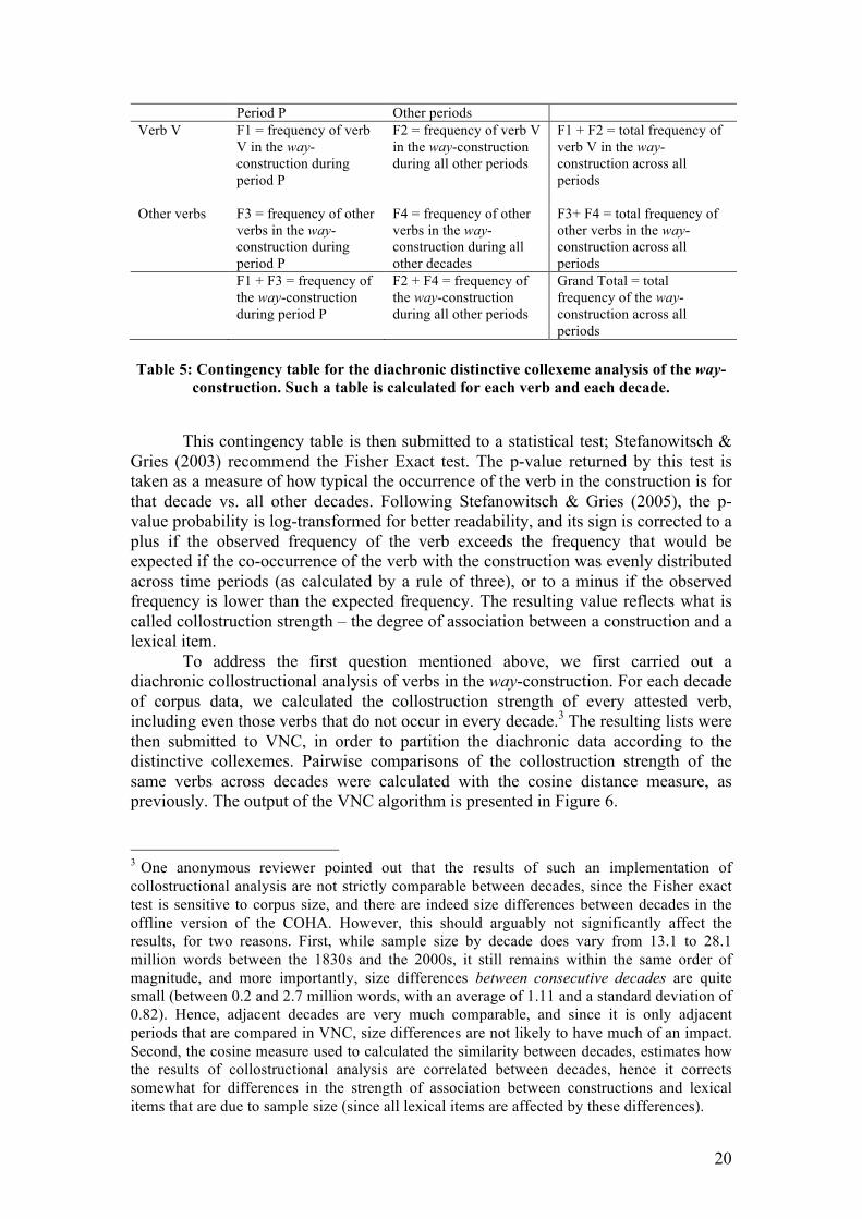
20

Period P Other periods Verb V F1 = frequency of verb

V in the way-construction during period P

F2 = frequency of verb V in the way-construction during all other periods

F1 + F2 = total frequency of verb V in the way-construction across all periods

Other verbs F3 = frequency of other verbs in the way-construction during period P

F4 = frequency of other verbs in the way-construction during all other decades

F3+ F4 = total frequency of other verbs in the way-construction across all periods

F1 + F3 = frequency of the way-construction during period P

F2 + F4 = frequency of the way-construction during all other periods

Grand Total = total frequency of the way-construction across all periods

Table 5: Contingency table for the diachronic distinctive collexeme analysis of the way-

construction. Such a table is calculated for each verb and each decade.

This contingency table is then submitted to a statistical test; Stefanowitsch &

Gries (2003) recommend the Fisher Exact test. The p-value returned by this test is taken as a measure of how typical the occurrence of the verb in the construction is for that decade vs. all other decades. Following Stefanowitsch & Gries (2005), the p-value probability is log-transformed for better readability, and its sign is corrected to a plus if the observed frequency of the verb exceeds the frequency that would be expected if the co-occurrence of the verb with the construction was evenly distributed across time periods (as calculated by a rule of three), or to a minus if the observed frequency is lower than the expected frequency. The resulting value reflects what is called collostruction strength – the degree of association between a construction and a lexical item.

To address the first question mentioned above, we first carried out a diachronic collostructional analysis of verbs in the way-construction. For each decade of corpus data, we calculated the collostruction strength of every attested verb, including even those verbs that do not occur in every decade.3 The resulting lists were then submitted to VNC, in order to partition the diachronic data according to the distinctive collexemes. Pairwise comparisons of the collostruction strength of the same verbs across decades were calculated with the cosine distance measure, as previously. The output of the VNC algorithm is presented in Figure 6. 3 One anonymous reviewer pointed out that the results of such an implementation of collostructional analysis are not strictly comparable between decades, since the Fisher exact test is sensitive to corpus size, and there are indeed size differences between decades in the offline version of the COHA. However, this should arguably not significantly affect the results, for two reasons. First, while sample size by decade does vary from 13.1 to 28.1 million words between the 1830s and the 2000s, it still remains within the same order of magnitude, and more importantly, size differences between consecutive decades are quite small (between 0.2 and 2.7 million words, with an average of 1.11 and a standard deviation of 0.82). Hence, adjacent decades are very much comparable, and since it is only adjacent periods that are compared in VNC, size differences are not likely to have much of an impact. Second, the cosine measure used to calculated the similarity between decades, estimates how the results of collostructional analysis are correlated between decades, hence it corrects somewhat for differences in the strength of association between constructions and lexical items that are due to sample size (since all lexical items are affected by these differences).

21

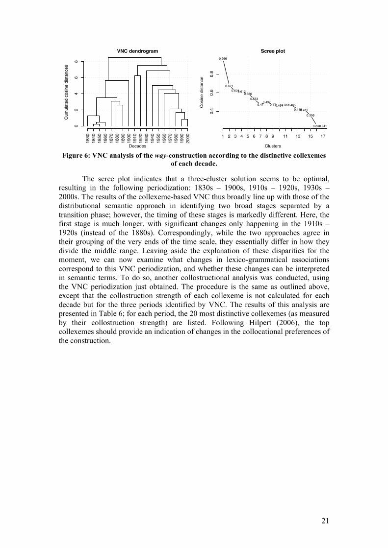
Figure 6: VNC analysis of the way-construction according to the distinctive collexemes

of each decade.

The scree plot indicates that a three-cluster solution seems to be optimal, resulting in the following periodization: 1830s – 1900s, 1910s – 1920s, 1930s – 2000s. The results of the collexeme-based VNC thus broadly line up with those of the distributional semantic approach in identifying two broad stages separated by a transition phase; however, the timing of these stages is markedly different. Here, the first stage is much longer, with significant changes only happening in the 1910s – 1920s (instead of the 1880s). Correspondingly, while the two approaches agree in their grouping of the very ends of the time scale, they essentially differ in how they divide the middle range. Leaving aside the explanation of these disparities for the moment, we can now examine what changes in lexico-grammatical associations correspond to this VNC periodization, and whether these changes can be interpreted in semantic terms. To do so, another collostructional analysis was conducted, using the VNC periodization just obtained. The procedure is the same as outlined above, except that the collostruction strength of each collexeme is not calculated for each decade but for the three periods identified by VNC. The results of this analysis are presented in Table 6; for each period, the 20 most distinctive collexemes (as measured by their collostruction strength) are listed. Following Hilpert (2006), the top collexemes should provide an indication of changes in the collocational preferences of the construction.

VNC dendrogram

Decades

Cum

ulat

ed c

osin

e di

stan

ces

1830

1840

1850

1860

1870

1880

1890

1900

1910

1920

1930

1940

1950

1960

1970

1980

1990

2000

02

46

8

Scree plot

Clusters

Cos

ine

dist

ance

1 2 3 4 5 6 7 8 9 11 13 15 17

0.4

0.6

0.8

0.966

0.6710.6210.612

0.5860.533

0.470.497

0.470.4610.4670.4650.4180.413

0.356

0.2410.241

22

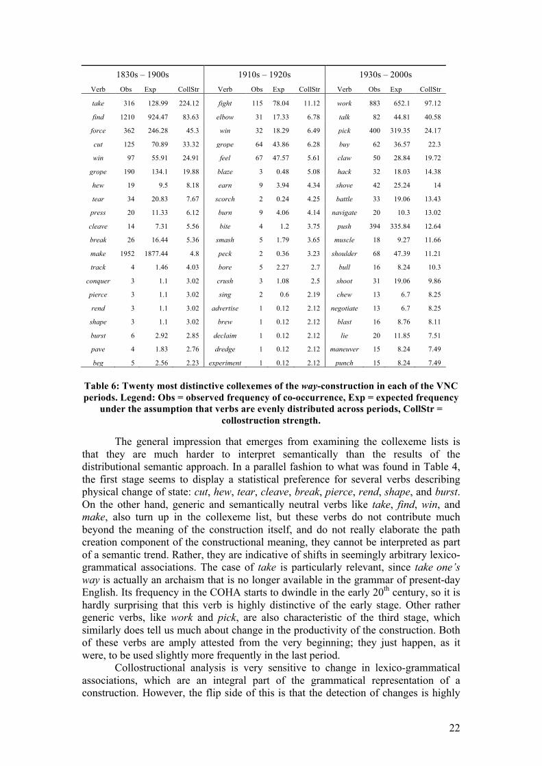
1830s – 1900s 1910s – 1920s 1930s – 2000s Verb Obs Exp CollStr Verb Obs Exp CollStr Verb Obs Exp CollStr

take 316 128.99 224.12 fight 115 78.04 11.12 work 883 652.1 97.12

find 1210 924.47 83.63 elbow 31 17.33 6.78 talk 82 44.81 40.58

force 362 246.28 45.3 win 32 18.29 6.49 pick 400 319.35 24.17

cut 125 70.89 33.32 grope 64 43.86 6.28 buy 62 36.57 22.3

win 97 55.91 24.91 feel 67 47.57 5.61 claw 50 28.84 19.72

grope 190 134.1 19.88 blaze 3 0.48 5.08 hack 32 18.03 14.38

hew 19 9.5 8.18 earn 9 3.94 4.34 shove 42 25.24 14

tear 34 20.83 7.67 scorch 2 0.24 4.25 battle 33 19.06 13.43

press 20 11.33 6.12 burn 9 4.06 4.14 navigate 20 10.3 13.02

cleave 14 7.31 5.56 bite 4 1.2 3.75 push 394 335.84 12.64

break 26 16.44 5.36 smash 5 1.79 3.65 muscle 18 9.27 11.66

make 1952 1877.44 4.8 peck 2 0.36 3.23 shoulder 68 47.39 11.21

track 4 1.46 4.03 bore 5 2.27 2.7 bull 16 8.24 10.3

conquer 3 1.1 3.02 crush 3 1.08 2.5 shoot 31 19.06 9.86

pierce 3 1.1 3.02 sing 2 0.6 2.19 chew 13 6.7 8.25

rend 3 1.1 3.02 advertise 1 0.12 2.12 negotiate 13 6.7 8.25

shape 3 1.1 3.02 brew 1 0.12 2.12 blast 16 8.76 8.11

burst 6 2.92 2.85 declaim 1 0.12 2.12 lie 20 11.85 7.51

pave 4 1.83 2.76 dredge 1 0.12 2.12 maneuver 15 8.24 7.49

beg 5 2.56 2.23 experiment 1 0.12 2.12 punch 15 8.24 7.49

Table 6: Twenty most distinctive collexemes of the way-construction in each of the VNC periods. Legend: Obs = observed frequency of co-occurrence, Exp = expected frequency

under the assumption that verbs are evenly distributed across periods, CollStr = collostruction strength.

The general impression that emerges from examining the collexeme lists is that they are much harder to interpret semantically than the results of the distributional semantic approach. In a parallel fashion to what was found in Table 4, the first stage seems to display a statistical preference for several verbs describing physical change of state: cut, hew, tear, cleave, break, pierce, rend, shape, and burst. On the other hand, generic and semantically neutral verbs like take, find, win, and make, also turn up in the collexeme list, but these verbs do not contribute much beyond the meaning of the construction itself, and do not really elaborate the path creation component of the constructional meaning, they cannot be interpreted as part of a semantic trend. Rather, they are indicative of shifts in seemingly arbitrary lexico-grammatical associations. The case of take is particularly relevant, since take one’s way is actually an archaism that is no longer available in the grammar of present-day English. Its frequency in the COHA starts to dwindle in the early 20th century, so it is hardly surprising that this verb is highly distinctive of the early stage. Other rather generic verbs, like work and pick, are also characteristic of the third stage, which similarly does tell us much about change in the productivity of the construction. Both of these verbs are amply attested from the very beginning; they just happen, as it were, to be used slightly more frequently in the last period.

Collostructional analysis is very sensitive to change in lexico-grammatical associations, which are an integral part of the grammatical representation of a construction. However, the flip side of this is that the detection of changes is highly

23

dependent on token frequency. As a result, the move towards more abstract verbs is much less prominently visible in the collostructional analysis, and is detected much later than in the distributional semantic approach. The only abstract collexemes are relatively frequent types, and only turn up in the collexeme list when they reach a certain prominence. For instance, talk and buy are attested from the late 19th century, albeit sporadically, but they only start occurring with reasonable frequency around the 1930s. It is also harder to identify abstract semantic classes from the collexeme list, as the abstract types make up an haphazard list including earn, sing, and the hapax legomena advertise, brew, declaim and experiment in the 1910s – 1920s, and talk, buy, negotiate and lie in the 1930s – 2000s. The status of the 1910s – 1920s as a transition period is also not as clear as that of the 1880s in the distributional semantic periodization, as it does not seem to involve distinctive classes, or fewer types than the surrounding periods in the same classes.

These observations pertaining to the differences in findings between collostructional analysis and the distributional semantic approach also explain the differences in the two periodizations that are put forward by VNC. Since collostructional analysis is sensitive to the distributional bias of certain individual verbs, a VNC periodization based on distinctive collexemes tends to group together periods in which the construction displays similar biases. By contrast, VNC periodization based on distributional semantics tends to group together periods in which the construction is instantiated by a semantically similar range of verbs, regardless of their frequency of occurrence. Even if a verb occurs only once in a period, it will affect the semantic representation of that period. Hence, while the distributional semantic approach disregards frequency information, it is able to capture semantic change in productivity with more detail than collostructional analysis. Yet, this is not to say that the former is necessarily superior to the latter in any situation. Most of the examples of constructions that were successfully analysed using diachronic collostructional analysis are high-frequency patterns with a strongly grammatical meaning: for instance, future constructions (e.g., will VERB, shall VERB; Hilpert 2008, Gries & Hilpert 2008), aspectual constructions (keep V-ing; Hilpert 2012a), and determiner constructions (many a NOUN; Hilpert 2012b). Collostructional analysis fares well with such constructions, not only because they tend to be highly frequent, but also because they tend to have a high degree of semantic openness; hence, uses of these constructions with unattested verbs do not sound as innovative as for constructions with a more restricted meaning, and the question is thus when and how the expansion into other semantic domains becomes established, rather than when new semantic domains start being attested at all (which might occur quite earlier than the former). To derive this kind of information, collostructional analysis is very well suited, and in fact, it is not clear if the distributional semantic approach would be more useful in the analysis of these high-frequency, strongly grammatical, and semantically more open constructions. Yet, this case study clearly shows that for lower-frequency constructions with a more “contentful” meaning, the distributional approach is more fruitful when it comes to the semantic analysis of their productivity.

5. Summary and conclusion The issue of periodization in diachronic studies relates to how to analyse historical usage data of a particular construction in terms of stages of language change. Manual periodization often poses methodological issues, as it is potentially subjective and is

24

not based on reproducible criteria. To address these issues, Gries & Hilpert (2008) created variability-based neighbour clustering (VNC), a variant of hierarchical clustering with the restriction that only time-adjacent periods can be grouped together, thus preserving the chronological order. So far, VNC has been used exclusively with quantitative measures, such as type and token frequencies and frequency distributions of lexical items. However, such measures only tell part of the story when it comes to the study of productivity change. In particular, they do not capture whether and how the lexical distribution of a construction becomes more semantically diverse. The present paper extends the scope of VNC by introducing a variant of the method based on representations of the semantic domain. In this variant, historical periods of a construction are grouped together if the construction is used with a similar semantic range of lexical items in both periods. The construction is characterized in each period by a semantic representation that combines the semantics of all words attested in a specific slot of the construction, as provided by a distributional semantic model that captures meaning of words as a function of their frequent lexical collocates in a large corpus of texts.

This method partitions the history of a construction according to qualitative stages of productivity corresponding to different sets of semantic classes attested in one of its lexical slots. Two case studies were presented to showcase distributional-semantic VNC: the first on the hell-construction (Hoeksema & Napoli 2008, Perek 2016) from its inception in the 1930s, and the way-construction (Goldberg 1995, Israel 1996, Perek 2016b) from the 1830s onwards, both drawing on data from the COHA (Davies 2012). In the first case study, it was found that distributional-semantic VNC appropriately captures the gradual expansion of the construction within two restricted central semantic domains, which aligns with previous research. By contrast, quantitative measures of productivity indicate two distinct stages that do not find any counterpart from a qualitative point of view. This shows that the historical development of quantitative aspects of a construction does not always match that of some of its qualitative aspects. The second case study was specifically aimed at contrasting the results of two forms of VNC: the present distributional semantic approach and one based on collostructional analysis (Gries & Stefanowitsch 2004, Hilpert 2012), a method that characterizes how typical the lexical fillers of a construction are through their frequency of occurrence in the contruction, and is often claimed to capture aspects of the semantics of constructions. The VNC periodization based on distributional semantics and the one based on collostructional analysis were found to overlap to some degree, but they also display substantial differences. In general, semantic change is measured with greater precision by the distributional approach, both regarding the nature of changes and their chronology. This finding probably owes to the fact that the collostructional approach heavily relies on significant variation in token frequency to measure change; consequently, changes that are not attested with sufficient frequency might stay under the radar, even if they are driven by many types. In this regard, the two approaches are to be seen as complementary: the distributional approach addresses some of the limitations of collostructional analysis, especially as it pertains to the analysis of low-frequency constructions, but the collostructional approach is still helpful in measuring change in lexico-grammatical associations, especially in the case of high-frequency constructions, which may or may not relate to a construction’s productivity in semantic terms.

In conclusion, the extension of VNC presented in this paper offers a useful addition to the range of available tools for quantitative studies of language change. It

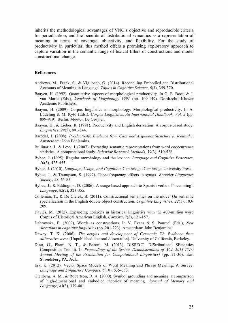
25

inherits the methodological advantages of VNC’s objective and reproducible criteria for periodization, and the benefits of distributional semantics as a representation of meaning in terms of coverage, objectivity, and flexibility. For the study of productivity in particular, this method offers a promising exploratory approach to capture variation in the semantic range of lexical fillers of constructions and model constructional change. References Andrews, M., Frank, S., & Vigliocco, G. (2014). Reconciling Embodied and Distributional

Accounts of Meaning in Language. Topics in Cognitive Science, 6(3), 359-370. Baayen, H. (1992). Quantitative aspects of morphological productivity. In G. E. Booij & J.

van Marle (Eds.), Yearbook of Morphology 1991 (pp. 109-149). Dordrecht: Kluwer Academic Publishers.

Baayen, H. (2009). Corpus linguistics in morphology: Morphological productivity. In A. Lüdeling & M. Kytö (Eds.), Corpus Linguistics. An International Handbook, Vol. 2 (pp. 899-919). Berlin: Mouton De Gruyter.

Baayen, H., & Lieber, R. (1991). Productivity and English derivation: A corpus-based study. Linguistics, 29(5), 801-844.

Barðdal, J. (2008). Productivity: Evidence from Case and Argument Structure in Icelandic. Amsterdam: John Benjamins.

Bullinaria, J., & Levy, J. (2007). Extracting semantic representations from word cooccurrence statistics: A computational study. Behavior Research Methods, 39(3), 510-526.

Bybee, J. (1995). Regular morphology and the lexicon. Language and Cognitive Processes, 10(5), 425-455.

Bybee, J. (2010). Language, Usage, and Cognition. Cambridge: Cambridge University Press. Bybee, J., & Thompson, S. (1997). Three frequency effects in syntax. Berkeley Linguistics

Society, 23, 65-85. Bybee, J., & Eddington, D. (2006). A usage-based approach to Spanish verbs of ‘becoming’.

Language, 82(2), 323-355. Colleman, T., & De Clerck, B. (2011). Constructional semantics on the move: On semantic

specialization in the English double object construction. Cognitive Linguistics, 22(1), 183-209.

Davies, M. (2012). Expanding horizons in historical linguistics with the 400-million word Corpus of Historical American English. Corpora, 7(2), 121-157.

Dąbrowska, E. (2009). Words as constructions. In V. Evans & S. Pourcel (Eds.), New directions in cognitive linguistics (pp. 201-223). Amsterdam: John Benjamins.

Dewey, T. K. (2006). The origins and development of Germanic V2: Evidence from alliterative verse (Unpublished doctoral dissertation). University of California, Berkeley.

Dinu, G., Pham, N. T., & Baroni, M. (2013). DISSECT: DIStributional SEmantics Composition Toolkit. In Proceedings of the System Demonstrations of ACL 2013 (51st Annual Meeting of the Association for Computational Linguistics) (pp. 31-36). East Stroudsburg PA: ACL.

Erk, K. (2012). Vector Space Models of Word Meaning and Phrase Meaning: A Survey. Language and Linguistics Compass, 6(10), 635-653.

Glenberg, A. M., & Robertson, D. A. (2000). Symbol grounding and meaning: a comparison of high-dimensional and embodied theories of meaning. Journal of Memory and Language, 43(3), 379-401.

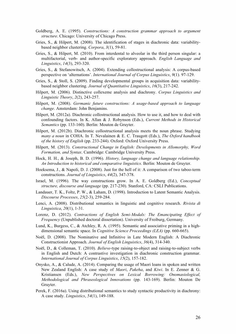
26

Goldberg, A. E. (1995). Constructions: A construction grammar approach to argument structure. Chicago: University of Chicago Press.

Gries, S., & Hilpert, M. (2008). The identification of stages in diachronic data: variability-based neighbor clustering. Corpora, 3(1), 59-81.

Gries, S., & Hilpert, M. (2010). From interdental to alveolar in the third person singular: a multifactorial, verb- and author-specific exploratory approach. English Language and Linguistics, 14(3), 293-320.

Gries, S., & Stefanowitsch, A. (2004). Extending collostructional analysis: A corpus-based perspective on ‘alternations’. International Journal of Corpus Linguistics, 9(1). 97-129.

Gries, S., & Stoll, S. (2009). Finding developmental groups in acquisition data: variability-based neighbor clustering. Journal of Quantitative Linguistics, 16(3), 217-242.

Hilpert, M. (2006). Distinctive collexeme analysis and diachrony. Corpus Linguistics and Linguistic Theory, 2(2), 243-257.

Hilpert, M. (2008). Germanic future constructions: A usage-based approach to language change. Amsterdam: John Benjamins.

Hilpert, M. (2012a). Diachronic collostructional analysis. How to use it, and how to deal with confounding factors. In K. Allan & J. Robynson (Eds.), Current Methods in Historical Semantics (pp. 133-160). Berlin: Mouton de Gruyter.

Hilpert, M. (2012b). Diachronic collostructional analysis meets the noun phrase. Studying many a noun in COHA. In T. Nevalainen & E. C. Traugott (Eds.), The Oxford handbook of the history of English (pp. 233-244). Oxford: Oxford University Press.

Hilpert, M. (2013). Constructional Change in English: Developments in Allomorphy, Word Formation, and Syntax. Cambridge: Cambridge University Press.

Hock, H. H., & Joseph, B. D. (1996). History, language change and language relationship. An Introduction to historical and comparative linguistics. Berlin: Mouton de Gruyter.

Hoeksema, J., & Napoli, D. J. (2008). Just for the hell of it: A comparison of two taboo-term constructions. Journal of Linguistics, 44(2), 347-378.

Israel, M. (1996). The way constructions grow. In A. E. Goldberg (Ed.), Conceptual structure, discourse and language (pp. 217-230). Stanford, CA: CSLI Publications.

Landauer, T. K., Foltz, P. W., & Laham, D. (1998). Introduction to Latent Semantic Analysis. Discourse Processes, 25(2-3), 259-284.

Lenci, A. (2008). Distributional semantics in linguistic and cognitive research. Rivista di Linguistica, 20(1), 1-31.

Lorenz, D. (2012). Contractions of English Semi-Modals: The Emancipating Effect of Frequency (Unpublished doctoral dissertation). University of Freiburg, Germany.

Lund, K., Burgess, C., & Atchley, R. A. (1995). Semantic and associative priming in a high-dimensional semantic space. In Cognitive Science Proceedings (LEA) (pp. 660-665).

Noël, D. (2008). The Nominative and Infinitive in Late Modern English: A Diachronic Constructionist Approach. Journal of English Linguistics, 36(4), 314-340.

Noël, D., & Colleman, T. (2010). Believe-type raising-to-object and raising-to-subject verbs in English and Dutch: A contrastive investigation in diachronic construction grammar. International Journal of Corpus Linguistics, 15(2), 157-182.

Onysko, A., & Calude, A. (2014). Comparing the usage of Maori loans in spoken and written New Zealand English: A case study of Maori, Pakeha, and Kiwi. In E. Zenner & G. Kristiansen (Eds.), New Perspectives on Lexical Borrowing: Onomasiological, Methodological and Phraseological Innovations (pp. 143-169). Berlin: Mouton De Gruyter.

Perek, F. (2016a). Using distributional semantics to study syntactic productivity in diachrony: A case study. Linguistics, 54(1), 149-188.

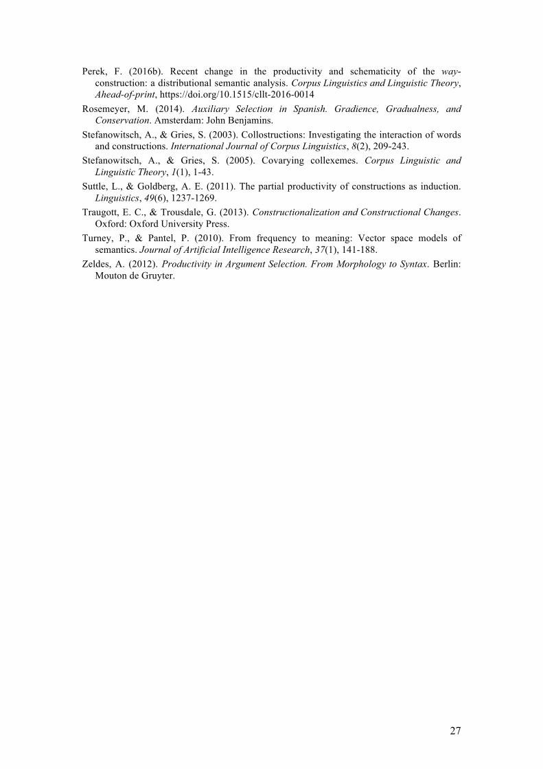
27

Perek, F. (2016b). Recent change in the productivity and schematicity of the way-construction: a distributional semantic analysis. Corpus Linguistics and Linguistic Theory, Ahead-of-print, https://doi.org/10.1515/cllt-2016-0014

Rosemeyer, M. (2014). Auxiliary Selection in Spanish. Gradience, Gradualness, and Conservation. Amsterdam: John Benjamins.

Stefanowitsch, A., & Gries, S. (2003). Collostructions: Investigating the interaction of words and constructions. International Journal of Corpus Linguistics, 8(2), 209-243.

Stefanowitsch, A., & Gries, S. (2005). Covarying collexemes. Corpus Linguistic and Linguistic Theory, 1(1), 1-43.

Suttle, L., & Goldberg, A. E. (2011). The partial productivity of constructions as induction. Linguistics, 49(6), 1237-1269.

Traugott, E. C., & Trousdale, G. (2013). Constructionalization and Constructional Changes. Oxford: Oxford University Press.

Turney, P., & Pantel, P. (2010). From frequency to meaning: Vector space models of semantics. Journal of Artificial Intelligence Research, 37(1), 141-188.

Zeldes, A. (2012). Productivity in Argument Selection. From Morphology to Syntax. Berlin: Mouton de Gruyter.