
A Distributed Architecture, FileSystem, & MapReducehas/CSE545/Slides/2.10-3.pdf · Rack 1 Rack 2....
75
A Distributed Architecture, FileSystem, & MapReduce Stony Brook University CSE545, Fall 2017
Transcript of A Distributed Architecture, FileSystem, & MapReducehas/CSE545/Slides/2.10-3.pdf · Rack 1 Rack 2....

A Distributed Architecture, FileSystem, & MapReduce
Stony Brook UniversityCSE545, Fall 2017

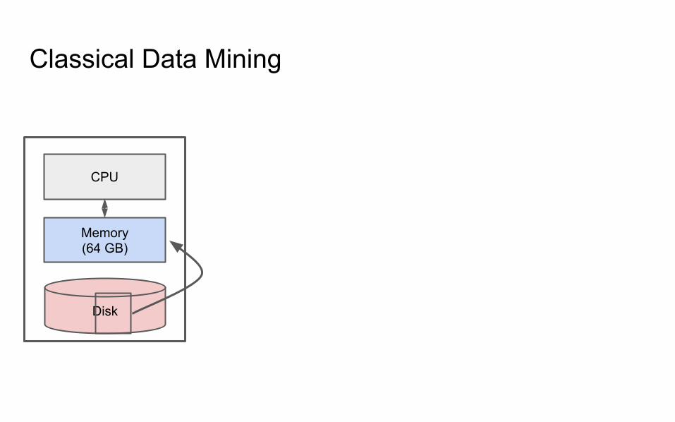
Classical Data Mining
CPU
Memory
Disk

Classical Data Mining
CPU
Memory(64 GB)
Disk
Classical Data Mining
CPU
Memory(64 GB)
Disk

Classical Data Mining
CPU
Memory(64 GB)
Disk

IO Bounded
Reading a word from disk versus main memory: 105 slower!
Reading many contiguously stored words is faster per word, but fast modern disksstill only reach 150MB/s for sequential reads.
IO Bound: biggest performance bottleneck is reading / writing to disk.
(starts around 100 GBs; ~10 minutes just to read).

Classical Big Data Analysis
Often focused on efficiently utilizing the disk.
e.g. Apache Lucene / Solr
Still bounded when needing to process all of a large file.
CPU
Memory
Disk

IO Bound
How to solve?

Distributed Architecture (Cluster)
CPU
Memory
Disk
CPU
Memory
Disk
CPU
Memory
Disk
...
Switch~1Gbps
CPU
Memory
Disk
CPU
Memory
Disk
CPU
Memory
Disk
...
Switch~1Gbps ...
Switch~10Gbps
Rack 1 Rack 2

Distributed Architecture (Cluster)In reality, modern setups often have multiple cpus and disks per server, but we will model as if one machineper cpu-disk pair.
CPU
Disk
CPU
Disk
CPU
Memory
Disk
...
...
CPU
Disk
CPU
Disk
CPU
Memory
Disk
...
...
Switch~1Gbps
...

Distributed Architecture (Cluster)
CPU
Memory
Disk
CPU
Memory
Disk
CPU
Memory
Disk
...
Switch~1Gbps
CPU
Memory
Disk
CPU
Memory
Disk
CPU
Memory
Disk
...
Switch~1Gbps ...
Switch~10Gbps
Rack 1 Rack 2

Challenges for IO Cluster Computing
1. Nodes fail1 in 1000 nodes fail a day
2. Network is a bottleneckTypically 1-10 Gb/s throughput
3. Traditional distributed programming is often ad-hoc and complicated

Challenges for IO Cluster Computing
1. Nodes fail1 in 1000 nodes fail a dayDuplicate Data
2. Network is a bottleneckTypically 1-10 Gb/s throughput Bring computation to nodes, rather than data to nodes.
3. Traditional distributed programming is often ad-hoc and complicatedStipulate a programming system that can easily be distributed
MapReduce Accomplishes

Distributed File System
Before we understand MapReduce, we need to understand the type of file system it is meant to run on.
The filesystem itself is largely responsible for much of the speed up MapReduce provides!

Characteristics for Big Data Tasks
Large files (i.e. >100 GB to TBs)
Reads are most common
No need to update in place (append preferred) CPU
Memory
Disk

Distributed File System
(e.g. Apache HadoopDFS, GoogleFS, EMRFS)
C, D: Two different files
(Leskovec at al., 2014; http://www.mmds.org/)
chunk server 1 chunk server 2 chunk server 3 chunk server n

Distributed File System
(e.g. Apache HadoopDFS, GoogleFS, EMRFS)
C, D: Two different files
(Leskovec at al., 2014; http://www.mmds.org/)
chunk server 1 chunk server 2 chunk server 3 chunk server n

Distributed File System
(e.g. Apache HadoopDFS, GoogleFS, EMRFS)
C, D: Two different files
(Leskovec at al., 2014; http://www.mmds.org/)
chunk server 1 chunk server 2 chunk server 3 chunk server n
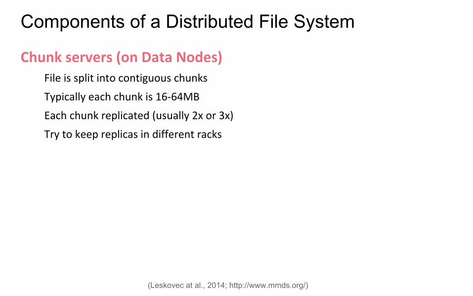
Components of a Distributed File System
Chunk servers (on Data Nodes)File is split into contiguous chunks
Typically each chunk is 16-64MB
Each chunk replicated (usually 2x or 3x)
Try to keep replicas in different racks
(Leskovec at al., 2014; http://www.mmds.org/)

Components of a Distributed File System
Chunk servers (on Data Nodes)File is split into contiguous chunks
Typically each chunk is 16-64MB
Each chunk replicated (usually 2x or 3x)
Try to keep replicas in different racks
Name node (aka master node)Stores metadata about where files are stored
Might be replicated or distributed across data nodes.
Client library for file accessTalks to master to find chunk servers
Connects directly to chunk servers to access data
(Leskovec at al., 2014; http://www.mmds.org/)
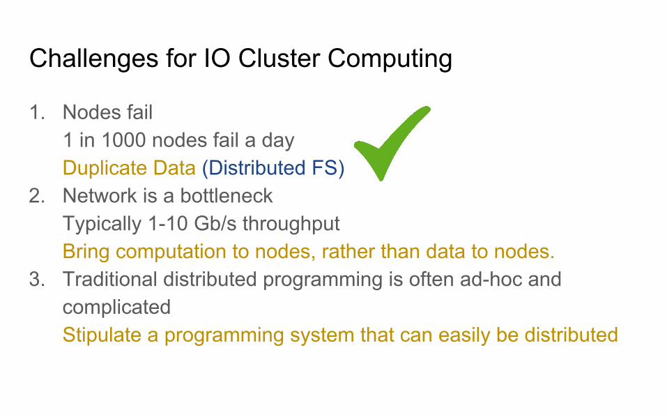
Challenges for IO Cluster Computing
1. Nodes fail1 in 1000 nodes fail a dayDuplicate Data (Distributed FS)
2. Network is a bottleneckTypically 1-10 Gb/s throughput Bring computation to nodes, rather than data to nodes.
3. Traditional distributed programming is often ad-hoc and complicatedStipulate a programming system that can easily be distributed

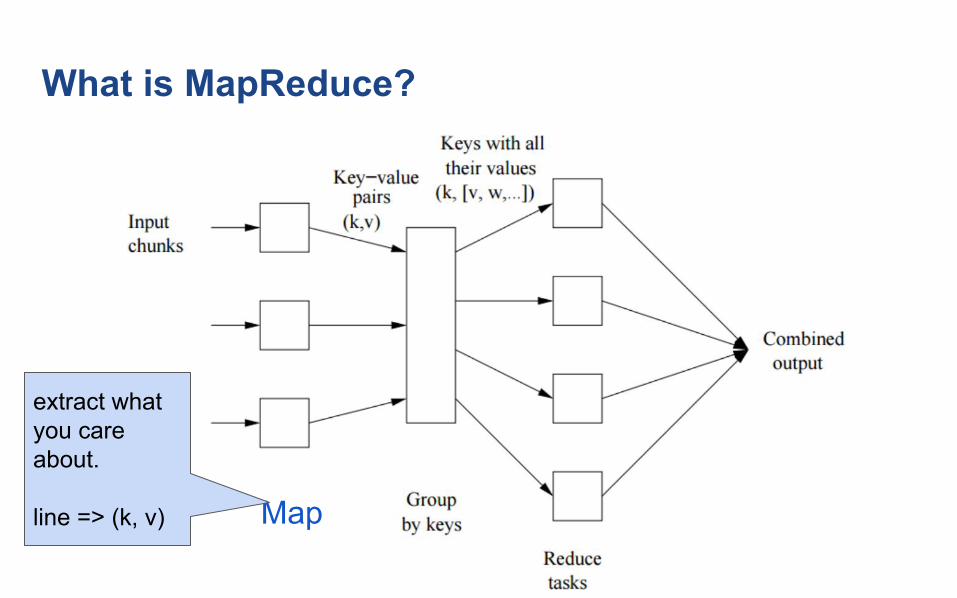
What is MapReduce?
1. A style of programming
input chunks => map tasks | group_by keys | reduce tasks => output
“|” is the linux “pipe” symbol: passes stdout from first process to stdin of next.
E.g. counting words:
tokenize(document) | sort | uniq -C

What is MapReduce?
1. A style of programming
input chunks => map tasks | group_by keys | reduce tasks => output
“|” is the linux “pipe” symbol: passes stdout from first process to stdin of next.
E.g. counting words:
tokenize(document) | sort | uniq -C
2. A system that distributes MapReduce style programs across a distributed file-system.
(e.g. Google’s internal “MapReduce” or apache.hadoop.mapreduce with hdfs)

What is MapReduce?
What is MapReduce?
Map
extract what you care about.
line => (k, v)

What is MapReduce?
Map
extract what you care about.
sort and shuffle
many (k, v) =>(k, [v1, v2]), ...

What is MapReduce?
Map
extract what you care about.
Reduce
aggregate, summarize
sort and shuffle

What is MapReduce?
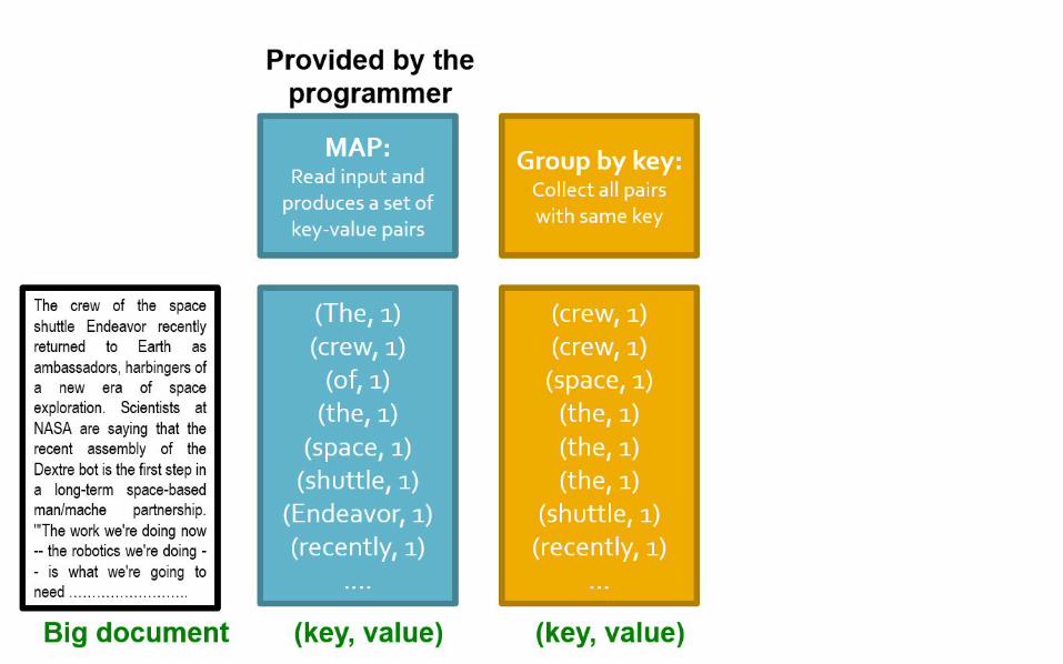
Map: (k,v) -> (k’, v’)*(Written by programmer)
Group by key: (k1’, v1’), (k2’, v2’), ... -> (k1’, (v1’, v’, …), (system handles) (k2’, (v1’, v’, …), …
Reduce: (k’, (v1’, v’, …)) -> (k’, v’’)*(Written by programmer)

Example: Word Count
tokenize(document) | sort | uniq -C

Example: Word Count
tokenize(document) | sort | uniq -C
Map: extract what you care about.
Reduce: aggregate, summarize
sort and shuffle

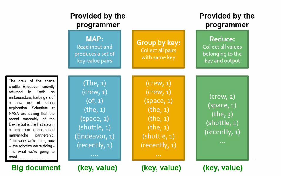

Example: Word Count
@abstractmethoddef map(k, v):
pass
@abstractmethoddef reduce(k, vs):
pass

Example: Word Count (version 1)
def map(k, v):for w in tokenize(v):
yield (w,1)
def reduce(k, vs):return len(vs)

Example: Word Count (version 2)
def map(k, v):counts = dict()for w in tokenize(v):
try: counts[w] += 1
except KeyError:counts[w] = 1
for item in counts.iteritems()yield item
def reduce(k, vs):return sum(vs)
counts each word within the chunk(try/except is faster than “if w in counts”)
sum of counts from different chunks

Challenges for IO Cluster Computing
1. Nodes fail1 in 1000 nodes fail a dayDuplicate Data (Distributed FS)
2. Network is a bottleneckTypically 1-10 Gb/s throughput (Sort & Shuffle)Bring computation to nodes, rather than data to nodes.
3. Traditional distributed programming is often ad-hoc and complicated Stipulate a programming system that can easily be distributed
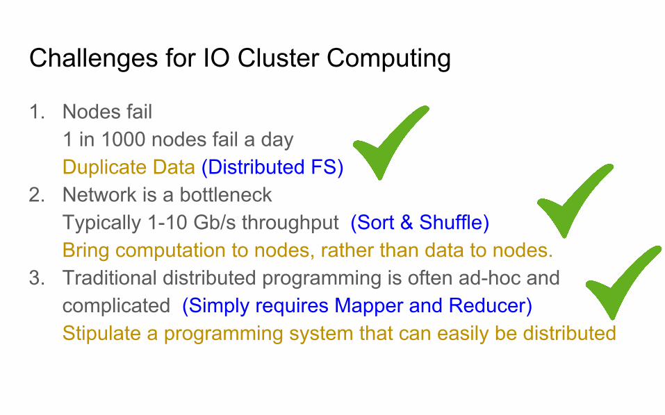
Challenges for IO Cluster Computing
1. Nodes fail1 in 1000 nodes fail a dayDuplicate Data (Distributed FS)
2. Network is a bottleneckTypically 1-10 Gb/s throughput (Sort & Shuffle)Bring computation to nodes, rather than data to nodes.
3. Traditional distributed programming is often ad-hoc and complicated (Simply requires Mapper and Reducer)Stipulate a programming system that can easily be distributed

Example: Relational Algebra
Select
Project
Union, Intersection, Difference
Natural Join
Grouping

Example: Relational Algebra
Select
Project
Union, Intersection, Difference
Natural Join
Grouping

Example: Relational Algebra
Select
R(A1,A2,A3,...), Relation R, Attributes A*
return only those attribute tuples where condition C is true

Example: Relational Algebra
Select
R(A1,A2,A3,...), Relation R, Attributes A*
return only those attribute tuples where condition C is true
def map(k, v): #v is list of attribute tuplesfor t in v:
if t satisfies C:yield (t, t)
def reduce(k, vs):
For each v in vs:
yield (k, v)

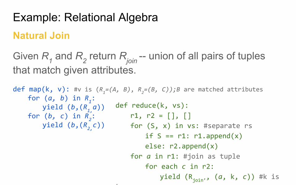
Example: Relational AlgebraNatural Join
Given R1 and R2 return Rjoin -- union of all pairs of tuples that match given attributes.

Example: Relational AlgebraNatural Join
Given R1 and R2 return Rjoin -- union of all pairs of tuples that match given attributes.
def map(k, v): #v is (R1=(A, B), R
2=(B, C));B are matched attributes
for (a, b) in R1:
yield (b,(R1,a))
for (b, c) in R2:
yield (b,(R2,c))
Example: Relational AlgebraNatural Join
Given R1 and R2 return Rjoin -- union of all pairs of tuples that match given attributes.
def map(k, v): #v is (R1=(A, B), R
2=(B, C));B are matched attributes
for (a, b) in R1:
yield (b,(R1,a))
for (b, c) in R2:
yield (b,(R2,c))
def reduce(k, vs):
r1, r2 = [], []
for (S, x) in vs: #separate rs
if S == r1: r1.append(x)
else: r2.append(x)
for a in r1: #join as tuple
for each c in r2:
yield (Rjoin’
, (a, k, c)) #k is
b

Data Flow

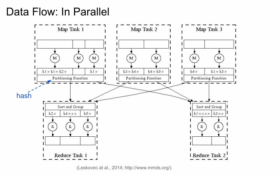
Data Flow: In Parallel
(Leskovec at al., 2014; http://www.mmds.org/)
Programmed
Programmed
hash

Data Flow
DFS Map Map’s Local FS Reduce DFS
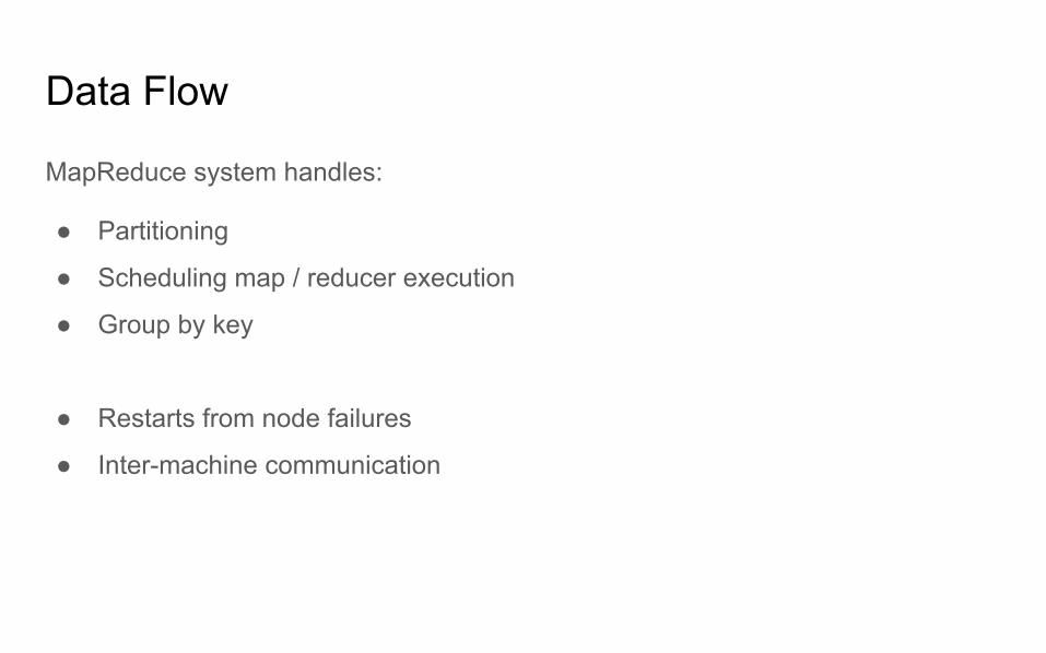
Data Flow
MapReduce system handles:
● Partitioning
● Scheduling map / reducer execution
● Group by key
● Restarts from node failures
● Inter-machine communication

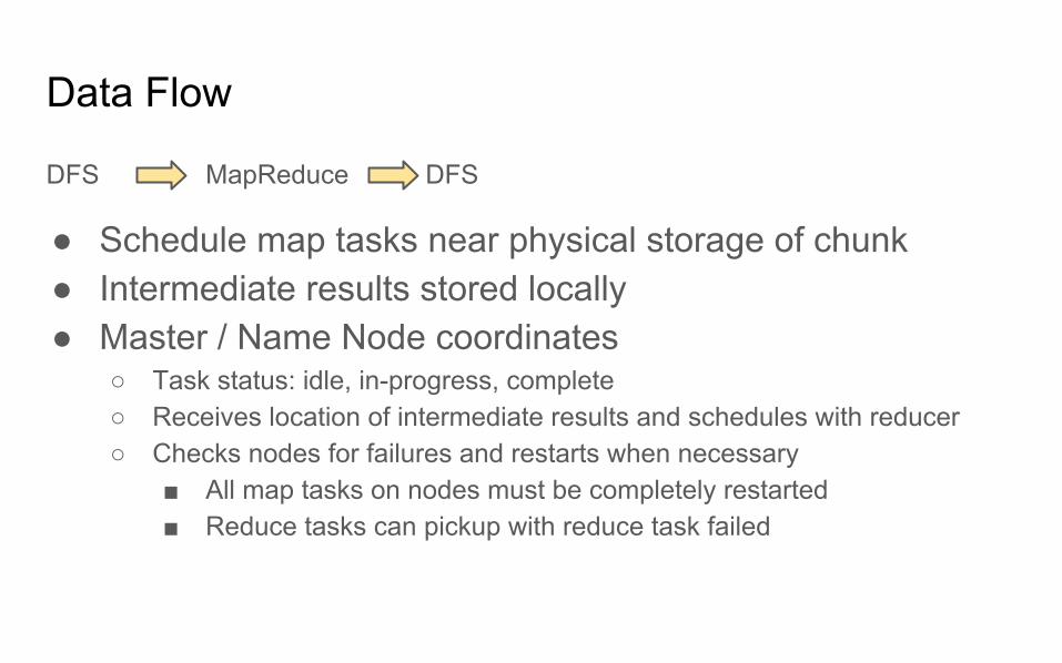
Data Flow
DFS MapReduce DFS
● Schedule map tasks near physical storage of chunk● Intermediate results stored locally● Master / Name Node coordinates
Data Flow
DFS MapReduce DFS
● Schedule map tasks near physical storage of chunk● Intermediate results stored locally● Master / Name Node coordinates
○ Task status: idle, in-progress, complete○ Receives location of intermediate results and schedules with reducer○ Checks nodes for failures and restarts when necessary
■ All map tasks on nodes must be completely restarted■ Reduce tasks can pickup with reduce task failed
DFS MapReduce DFS MapReduce DFS

Data Flow
Skew: The degree to which certain tasks end up taking much longer than others.
Handled with:
● More reducers than reduce tasks● More reduce tasks than nodes

Data Flow
Key Question: How many Map and Reduce jobs?

Data Flow
Key Question: How many Map and Reduce jobs?
M: map tasks, R: reducer tasks
A: If possible, one chunk per map task
and M >> |nodes| ≈≈ |cores|
(better handling of node failures, better load balancing)
R < M
(reduces number of parts stored in DFS)

Can redistribute these tasks to other nodes
Data Flow Reduce Task
node1
node2
node3
node4
node5
Reduce tasks represented by time to complete task
(some tasks take much longer)
node1
node2
node3
node4
node5
Reduce tasks represented by time to complete task
(some tasks take much longer)
version 1: few reduce tasks(same number of reduce tasks as nodes)
version 2: more reduce tasks(more reduce tasks than nodes)
node1
node2
node3
node4
node5
timetimetime
(the last task now completes much earlier )
Last task completed

Communication Cost Model
How to assess performance?
(1) Computation: Map + Reduce + System Tasks
(2) Communication: Moving (key, value) pairs

Communication Cost Model
How to assess performance?
(1) Computation: Map + Reduce + System Tasks
(2) Communication: Moving (key, value) pairs
Ultimate Goal: wall-clock Time.
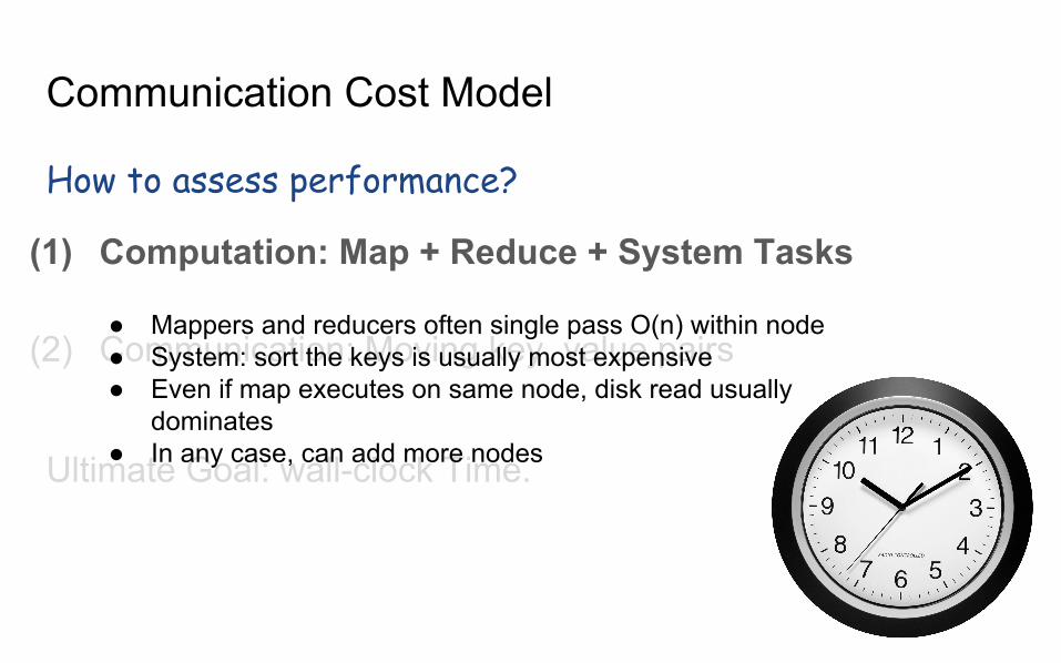
Communication Cost Model
How to assess performance?
(1) Computation: Map + Reduce + System Tasks
(2) Communication: Moving key, value pairs
Ultimate Goal: wall-clock Time.
● Mappers and reducers often single pass O(n) within node● System: sort the keys is usually most expensive● Even if map executes on same node, disk read usually
dominates● In any case, can add more nodes

Communication Cost Model
How to assess performance?
(1) Computation: Map + Reduce + System Tasks
(2) Communication: Moving key, value pairs
Ultimate Goal: wall-clock Time.
Often dominates computation. ● Connection speeds: 1-10 gigabits per sec;
HD read: 50-150 gigabytes per sec● Even reading from disk to memory typically takes longer than
operating on the data.

Communication Cost Model
How to assess performance?
(1) Computation: Map + Reduce + System Tasks
(2) Communication: Moving key, value pairs
Ultimate Goal: wall-clock Time.
Communication Cost = input size + (sum of size of all map-to-reducer files)
Often dominates computation. ● Connection speeds: 1-10 gigabits per sec;
HD read: 50-150 gigabytes per sec● Even reading from disk to memory typically takes longer than
operating on the data.

Communication Cost Model
How to assess performance?
(1) Computation: Map + Reduce + System Tasks
(2) Communication: Moving key, value pairs
Ultimate Goal: wall-clock Time.
Often dominates computation. ● Connection speeds: 1-10 gigabits per sec;
HD read: 50-150 gigabytes per sec● Even reading from disk to memory typically takes longer than
operating on the data.● Output from reducer ignored because it’s either small (finished
summarizing data) or being passed to another mapreduce job.
Communication Cost = input size + (sum of size of all map-to-reducer files)
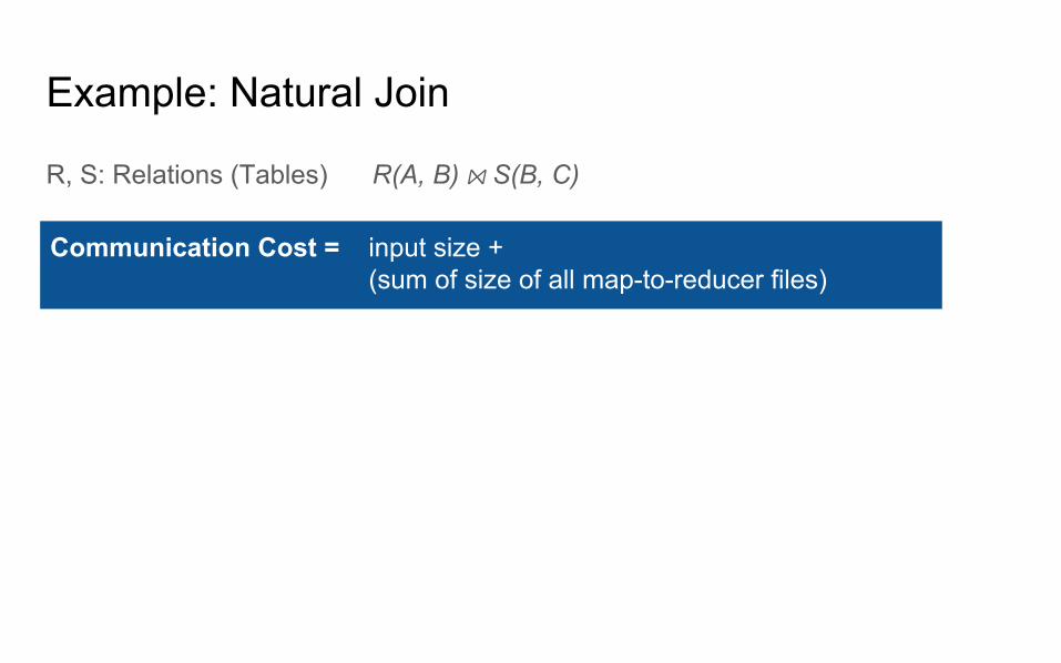
Example: Natural Join
R, S: Relations (Tables) R(A, B) ⨝ S(B, C)
Communication Cost = input size + (sum of size of all map-to-reducer files)

Example: Natural Join
R, S: Relations (Tables) R(A, B) ⨝ S(B, C)
Communication Cost = input size + (sum of size of all map-to-reducer files)
= |R| + |S| + (|R| + |S|)
= O(|R| + |S|)
def map(k, v): for (a, b) in R:
yield (b,(‘R’,a))
for (b, c) in S:yield (b,(‘S’
,c))
def reduce(k, vs):
r1, r2 = [], []
for (rel, x) in vs: #separate rs
if rel == ‘R’: r1.append(x)
else: r2.append(x)
for a in r1: #join as tuple
for each c in r2:
yield (Rjoin’
, (a, k, c)) #k is
b

Exercise:
Calculate Communication Cost for “Matrix Multiplication with One MapReduce Step” (see MMDS section 2.3.10)
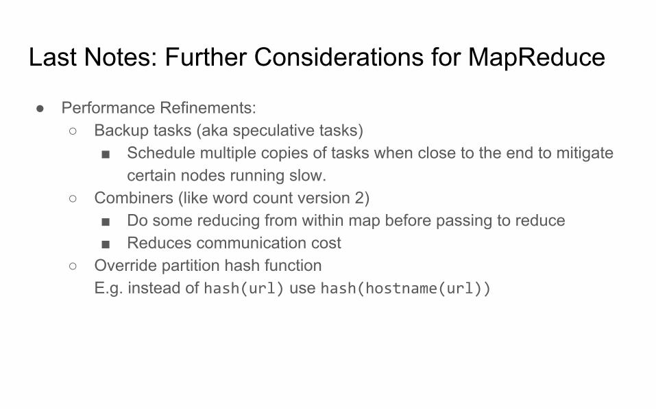
Last Notes: Further Considerations for MapReduce
● Performance Refinements:○ Backup tasks (aka speculative tasks)
■ Schedule multiple copies of tasks when close to the end to mitigate certain nodes running slow.
○ Combiners (like word count version 2)■ Do some reducing from within map before passing to reduce■ Reduces communication cost
○ Override partition hash functionE.g. instead of hash(url) use hash(hostname(url))
![Distributed Join Algorithms on Thousands of Cores · multi-core machines [1, 3, 5, 9, 27] and rack-scale data processing systems [6, 33] has shown that carefully tuned distributed](https://static.fdocuments.in/doc/165x107/5e71f3dc3bad8105c240e5ba/distributed-join-algorithms-on-thousands-of-multi-core-machines-1-3-5-9-27.jpg)