A Distance Measure for the Analysis ofPolar Opinion Dynamics in Social Networks

Victor AmelkinUniversity of California

Santa Barbara, CAvictor@cs.ucsb.edu

Ambuj K. SinghUniversity of California

Santa Barbara, CAambuj@cs.ucsb.edu

Petko BogdanovUniversity at Albany – SUNY

Albany, NYpbogdanov@albany.edu

ABSTRACTAnalysis of opinion dynamics in social networks plays an im-portant role in today’s life. For applications such as predict-ing users’ political preference, it is particularly importantto be able to analyze the dynamics of competing opinions.While observing the evolution of polar opinions of a socialnetwork’s users over time, can we tell when the network “be-haved” abnormally? Furthermore, can we predict how theopinions of the users will change in the future? Do opinionsevolve according to existing network opinion dynamics mod-els? To answer such questions, it is not sufficient to studyindividual user behavior, since opinions can spread far be-yond users’ egonets. We need a method to analyze opiniondynamics of all network users simultaneously and capturethe effect of individuals’ behavior on the global evolutionpattern of the social network.

In this work, we introduce Social Network Distance (SND)—a distance measure that quantifies the “cost” of evolutionof one snapshot of a social network into another snapshotunder various models of polar opinion propagation. SNDhas a rich semantics of a transportation problem, yet, iscomputable in time linear in the number of users, whichmakes SND applicable to the analysis of large-scale onlinesocial networks. In our experiments with synthetic and real-world Twitter data, we demonstrate the utility of our dis-tance measure for anomalous event detection. It achievesa true positive rate of 0.83, twice as high as that of alter-natives. When employed for opinion prediction in Twitter,our method’s accuracy is 75.63%, which is 7.5% higher thanthat of the next best method.

Code: http://cs.ucsb.edu/~victor/pub/ucsb/dbl/snd/

1. INTRODUCTIONAnalysis of people’s opinions plays an important role in

today’s life, and social networks provide a great platformfor such research. Businesses are interested in advertisingtheir products in social networks relying on viral marketing.Political strategists are interested in predicting an electionoutcome based on the observed sentiment change of a sam-ple of voters. Mass media and security analysts may beinterested in a timely discovery of anomalies based on howa social network “behaves”. Thus, it is important to havemethods for the analysis of how user opinions evolve in asocial network.

How can we quantify the change in opinions of users withrespect to their expected behavior in a social network? Canwe distinguish opinion shifts caused by in-network user in-

teraction from those caused by factors external to the net-work? To answer such questions, we need a distance mea-sure that explicitly models opinion dynamics, incorporatingboth the distribution of user opinions at two time instancesand the network structure that defines the pathways foropinion dissemination. In this work, we develop such a dis-tance measure for snapshots of a social network and employit for the analysis of competing opinion dynamics.

While the dynamics of a social network can be charac-terized by evolution of both the network’s structure anduser opinions [23], in this paper we focus on the opiniondynamics. We assume that there are two polar opinions inthe network, positive “+” and negative “−”. Users havingno or an unknown opinion are termed neutral, while thoseexpressing opinion—active. A network state is comprisedof the opinions of all network users at a given time. Po-lar opinions compete in that a user having a positive opin-ion is unlikely to enthusiastically spread information aboutthe adverse negative opinion, yet, would spread informationabout the friendly positive opinion“at a discount cost”. Suchcompetition may arise when the notions the opinions relateto are inherently competing. For example, in an election,the voters leaning toward one political party are unlikely tospread positive rumors about the competing party. Anotherexample is viral marketing, where the consumers who favorsmartphones of one brand may readily express their affectionto it, but may be unwilling to praise the competing brand.

Given a time series of network states, we address the appli-cations of detecting anomalous network states and predict-ing opinions of individual users. For the first application, weanswer the question of which network states are anomalouswith respect to the observed evolution of the network. Forthe second application, we predict currently unknown opin-ions of selected users in the network based on the network’sobserved past and present behavior.

The analysis of a time series of network states is, how-ever, complicated, because network states do not naturallybelong to any vector space, and the existing time series anal-ysis techniques cannot be readily applied. Our approach isto treat network states as members of a metric space in-duced by a distance measure governed by both the network’sstructure and user opinions. We design a semantically andmathematically appealing as well as efficiently computabledistance measure Social Network Distance (SND) for thecomparison of social network states containing polar opin-ions, and demonstrate its applicability to the analysis ofreal-world data.

To quantify the dissimilarity between network states, SND

1

arX

iv:1

510.

0505

8v1

[cs

.SI]

17

Oct

201

5

takes into account how information propagates in the net-work. A change of a given user’s opinion from, say, neutralto positive, contributes to the overall distance between thecorresponding network states by reflecting the likelihood ofthis user’s opinion change based on the opinions and loca-tions of other users in the network under a chosen model ofpolar opinion dynamics. However, since the network usersinteract, the distance measure needs to consider the opin-ion shifts of all users simultaneously. Thus, we define SNDas a transportation problem that models opinion spread andadoption in the network. In particular, by making the trans-portation costs dependent on both the network’s topologyand the opinions of the users conducting information in thenetwork, we capture the competitive aspect of polar opinionpropagation.

The summary of our contributions is as follows:• We propose SND—the first distance measure suitable forcomparison of social network states containing competingopinions under various models of opinion dynamics.• We develop a scalable method to precisely compute SNDin time linear in the number of users in the network, thus,making SND applicable to the analysis of real-world onlinesocial networks.• We demonstrate the applicability of our distance measureusing both synthetic and real-world data from Twitter. Indetecting anomalous states of a social network, SND is supe-rior to other distance measures in discovering controversialevents that have polarized the society. In user opinion pre-diction experiments, SND also outperforms competitors interms of prediction accuracy.

2. EARTH MOVER’S DISTANCE ANDNETWORK STATE COMPARISON

A good distance measure for the states of a social networkshould take into account the specifics of polar opinion prop-agation in a network. For example, a user having opinion“+” should not actively participate in the dissemination ofopinion “−”, or, at least, the dissemination of an adverseopinion should incur a large cost. On the other hand, thisuser should disseminate friendly opinion “+” at a cost lowerthan the cost a neutral user would incur. Thus, we proposeto address the problem of comparing states of a social net-work as a transportation problem where the costs of opinionpropagation are defined based on the shortest paths betweenthe users in the network, computed taking into account boththe network structure and the user opinions.

This high-level intuition about network state comparisonas an opinion transportation problem inadvertently leads usto one of the well-studied distance measures—Earth Mover’sDistance (EMD). Originally, defined as a dissimilarity mea-sure for histograms [25], EMD can be used for the compari-son of network states viewed as histograms, with histogrambins’ values quantifying individual user opinions. Intuitively,EMD measures the costs of optimal transformation of onehistogram into another with respect to the ground distancespecifying the costs of moving mass between bins. In ourcase, the ground distance is defined based on the shortestpaths between the users of the network, where the shortestpaths depend on both the network’s topology as well as theopinions of the users facilitating opinion propagation.

Formally, given two real-valued histograms P = [P1, . . . , Pn]and Q = [Q1, . . . , Qm], EMD between them with respect toa cross-bin ground distance Dijn×m is defined as the so-

lution to the problem of optimal mass transportation fromthe bins of P (suppliers) to the bins of Q (consumers) withrespect to transportation costs D.

EMD(P,Q,D) =

n∑i=1

m∑j=1

Dij fij/ n∑

i=1

m∑j=1

fij , (1)

where fijn×m is an optimal transportation plan in thefollowing transportation problem:

n∑i=1

m∑j=1

fijDij → min,

n∑i=1

m∑j=1

fij = min

n∑i=1

Pi,

m∑j=1

Qj

,

fij ≥ 0,

m∑j=1

fij ≤ Pi,n∑i=1

fij ≤ Qj , (1 ≤ i ≤ n, 1 ≤ j ≤ m).

EMD is attractive not only because its ground distancecan capture how opinions propagate in the underlying net-work, but it is also driven by node states rather than net-work topology, is spatially-sensitive, and metric under thefollowing conditions.

Theorem 1. (Rubner et al. [25]) If all histograms un-der comparison have equal total masses, and the underlyingground distance is metric, then EMD is metric.

In the following section, we use EMD to construct a distancemeasure for network states containing polar opinions.

3. DISTANCE MEASURE FOR NETWORKSTATES WITH POLAR OPINIONS

Given a network G = 〈V,E〉, where V (|V | = n) is the setof nodes (users) and E is the set of edges (social ties), wewant to compute the distance between two of its states P =[P1, . . . , Pn]T and Q = [Q1, . . . , Qn]T . While generalizationsare possible, we use an intuitive and simple scheme for polaropinion quantification: if user i has opinion “+” in networkstate P , then Pi = +1; Pi = −1 if the user’s opinion is “−”;and Pi = 0 if the user is neutral1.

Despite the appeal of EMD, it is not readily applicableto the comparison of network states P and Q, since (i) theusers’ behavior may change in the process of opinion propa-gation, while a transportation problem underlying EMD op-erates with static transportation costs; (ii) EMD is definedfor histograms of a homogeneous quantity, while P and Qcontain both positive and negative values; and (iii) it is notclear how to incorporate the node states into the definitionof the ground distance. In order to define our Social Net-work Distance (SND), we address these three problems inwhat follows.(i) SND as a transportation problem. For two givenusers u and v, not necessarily being immediate neighborsin the network, the cost of v’s adopting opinion from u de-pends not only on the states and locations of u and v in thenetwork, but also on the states of the users through whichu’s opinion can reach v.

In Fig. 1.a, user v3 having opinion “+” affects the cost ofpropagating opinion “−” from user v1 to user v4. In Fig. 1.b,however, user v3 is initially neutral, but can become active in

1 There is a great body of research on methods for opin-ion classification based on user-generated content. In thiswork, however, we assume that we have access only to thequantified opinions, and no access to the user-generated con-tent (e.g., tweets), which may be unavailable due to privacyreasons.

2

v1

- +v2

v3

v4 v

1

-v2

v3

v4

+

a) b)

v5

v6

Figure 1: Transitive opinion propagation in a social network.The solid and dashed arrows represent social ties and opinionflow, respectively.

the process of v5’s propagating “+” to v6 before opinion “−”from v1 reaches v3, thereby, impeding the spread of“−” fromv1 to v4. In order to pose SND as a transportation problem,we will assume that the costs of opinion propagation dependonly on the opinions of the currently active users, takingno account of the potential change of user opinions in theprocess of opinion transportation.

(ii) Handling polar opinions. We design SND to measurethe optimal cost of transforming one network state G1 intoanother network state G2 by the means of opinion trans-portation. The active users of G1 are the suppliers andthose in G2 are the consumers in the transportation prob-lem setting. In defining the transportation costs, we assumethat users adopting, say, opinion “+”, in G2 are affected byothers of the same opinion during the propagation. Simi-larly, suppliers only propagate opinions to the consumers ofthe same type. Thus, the set of constraints in the trans-portation problem can be divided into two non-overlappingsubsets for two kinds of opinions. Consequently, the prob-lem of optimal transportation of opinions from suppliers ofG1 to consumers of G2 can be split into two transportationproblems: one for transporting the opinions of each kind.

(iii) Defining the ground distance. The cost of opinionpropagation from user u to user v depends on their topologi-cal proximity, how frequently they communicate, persuasive-ness, and stubbornness of u and v as well as the users “sep-arating” them. Formally, the ground distance D(Gi, op) ∈R+n×n, reflecting the costs of propagating opinion op througha network in state Gi, is a matrix containing the lengths ofthe shortest paths in a network with its adjacency matrixdefined as:

Aext(Gi, op) =

− log P(Gi, op)− log Pin(Gi, op)− log Pout(Gi, op), (2)

where the summands on the right are n-by-n matrices oflog-probabilities of communication, opinion adoption, andopinion spreading, respectively. Probabilities P(Gi, op) canbe defined as the relative frequencies of communication be-tween users. In the absence of such information, we set− log P(Gi, op) to be the connectivity matrix of the network,penalizing for the users’ topological remoteness. Opinionadoption probabilities Pin(Gi, op) reflect users’ susceptibil-ity/stubbornness [28]. If such information is unavailable, foreach existing edge 〈u, v〉, we set Pinuv = 1, so that all usersare non-stubborn and equally receptive to persuasion. Fi-nally, the opinion spreading penalties − log Pout(Gi, op) aredefined based on a particular opinion dynamics model. Sev-eral ways to make such an assignment are described below.

Model-agnostic Opinion Propagation: If there is no evi-dence that opinions evolve in the network according to aspecific opinion dynamics model, then the opinion spread-

ing penalties can be defined as

− log Poutuv (Gi, op) =

cadverse if Gi[u] 6= op ∨Gi[v] = −op,cneutral if Gi[u] = 0,

cfriendly if Gi[u] = op,

where cadverse, cneutral, cfriendly are constant penalties forspreading opinion op by the users having respectively ad-verse, neutral, or friendly opinion relative to op, and Gi[u]is the opinion of user u in network state Gi. This simple def-inition implies that users willingly spread opinions similar totheir own (cfriendly is small); are unwilling to spread adverseopinions (cadverse is large); with neutral users’ behavior be-ing somewhere in-between (cfriendly < cneutral < cadverse).

Alternatively, Pout(Gi, op) can be defined via one of theexisting opinion dynamics models discussed next.

Independent Cascade Model: The distance-based model ofCarnes et al. [7] is a version of Independent Cascade Modelcapturing opinion competition. In this model, we have twosets of initial adopters I+, I− of opinions “+” and “−”, re-spectively, with I = I+∪I−. Each edge 〈u, v〉 is labeled withan activation probability puv (which can be learned from theobserved data [13]) and a distance duv. If we denote by dv(I)the shortest distance from any user of set I to user v withrespect to edge distances duv, and denote by pa(Gi, v) thesum of edge activation probabilities puv taken over all activeusers u in Gi such that dv(u) = dv(I), then

Poutuv (Gi, op) =

0 if dv(u) > dv(I),

1 if Gi[u] = op ∧Gi[v] = op,max(0,puv−ε)pa(Gi,v)

if Gi[u] = op ∧Gi[v] = 0,

ε otherwise.

In the original model of [7], ε = 0, that is, neutral userscannot infect others, and active users do not drop their opin-ions or spread competing opinions. If, however, we comparenetwork states with respect to the original model, then manynetwork states derived from real-world data would be at dis-tance +∞ from each other, either due to the lack of knowl-edge about the network (an edge has not been observed or auser’s opinion has been misclassified) or due to an imperfectfit of the model and the data. Instead of just declaring twonetwork states as qualitatively unreachable, we always wantto quantify the distance between them, and, thus, assignsome negligible probabilities ε to the events that the modelposits as impossible.

Linear Threshold Model: A version of Linear ThresholdModel supporting opinion competition has been proposed byBorodin et al. [5]. In this model, each edge 〈u, v〉 is weightedwith ωuv reflecting the amount of influence u has over v; andeach user u has an in-advance chosen constant threshold θu.If we denote by N in(Gi, v) the set of in-neighbors of v activein Gi, and by Ωin the sum of ωxv over all x ∈ N in(Gi, v),then

Poutuv (Gi, op) =

0 if u /∈ N in(Gi, v),

1 if Gi[u] = op ∧Gi[v] = op,(1−ε)ωuv

Ωin if Gi[u] = op ∧Gi[v] = 0 ∧ Ωin ≥ θv ,ε otherwise.

Having addressed challenges (i)-(iii), we are now ready toformally define SND.

In general, the network’s structure might have changedbetween the times corresponding to the two network statesunder comparison [23], but defining the ground distance foreach pair of users over a different network would incur an

3

unacceptably high time complexity of the resulting distancemeasure. Thus, for time-ordered network states G1 andG2, one can define the ground distance based on the net-work structure corresponding to the earlier network stateG1. However, to make SND applicable to time-unorderednetwork states as well, we define SND based on bothD(G1, op)and D(G2, op) as follows.

SND(G1, G2) =1

2× [ (3)

EMD(G+1 , G

+2 , D(G1,+)) + EMD(G−1 , G

−2 , D(G1,−))+

EMD(G+2 , G

+1 , D(G2,+)) + EMD(G−2 , G

−1 , D(G2,−))],

where users having opinion “−” are considered neutral inG+i , users having opinion “+” are neutral in G−i , and EMD

is the original Earth Mover’s Distance [25] that will furtherbe replaced with its generalization EMD? designed in thenext section. Since SND is a linear combination of severalinstances of EMD, then SND preserves most mathematicalproperties, and, in particular, metricity of the chosen EMD.

4. GENERALIZED EARTH MOVER’SDISTANCE

The original EMD [25] is limited in that it cannot ade-quately compare histograms having different total mass—itignores the mass mismatch, assigning a small distance valueto a pair of a light and a heavy histograms. However, if wethink about two histograms corresponding to the states of asocial network, one with a few and another one with manyactive users, then we expect the distance between such his-tograms to be large. In real-world data, even consecutivenetwork states observe a widely varying number of activeusers, making the challenge of comparing histograms withtotal mass mismatch well pronounced.

There are several extensions of EMD that address theabove mentioned limitation. One of them, EMD [24], aug-ments EMD with an additive mass mismatch penalty as fol-lows

EMD(P,Q,D) = EMD(P,Q,D) ·min∑

Pi,∑

Qj

+

+ α ·max Dij ·∣∣∑Pi −

∑Qj∣∣,

where EMD is the original Earth Mover’s Distance, andα is a constant parameter. The second summand repre-sents the mass mismatch penalty that depends only on themagnitude of the mass mismatch and the maximum grounddistance, thereby, being unable to capture the fine details ofthe network’s structure D can depend upon. This is, how-ever, inadequate for the comparison of the states of a socialnetwork, because the network’s behavior depends not onlyon the number of new activations, but also on where thesenewly activated users are located in the network.

Another EMD version, namely, EMDα [18], extends eachhistogram with an extra bin (“the bank bin”) whose value ischosen so that the total masses of the histograms becomeequal. An example of such an extension is shown in Fig. 2.Formally, EMDα is defined as follows.

P1

P2

P3

γ γ

γ

Q1

Q2

Q3

γ γ

γ

Figure 2: Histograms P and Q defined over the same net-work are extended with bank bins, whose capacities are cho-

sen, so that the total masses of the extended histograms P

and Q are equal. The ground distances Dbank,i = Di,bank =γ from and to the bank bin are uniformly defined basedon the largest ground distance between the initially presentbins.

P = [P1, . . . , Pn], Q = [Q1, . . . , Qn],

Pbank =

n∑j=1

Qj , P = [P, Pn+1 = Pbank] ,

Qbank =

n∑i=1

Pi, Q = [Q,Qn+1 = Qbank] ,

D =

Dn×n

|αmax

i,jDij|

— αmaxi,jDij — 0

,

EMDα(P,Q) = EMD(P , Q, D) ·

(n∑i=1

Pi +

n∑j=1

Qj

).

However, as we establish in Theorem 2, EMDα is equivalent

to EMD and, hence, is also unsuitable for the comparison ofsocial network states.

Theorem 2. If ground distance D ∈ Rn×n and param-

eter α ∈ R+ are chosen such that both EMDα and EMDare metric, that is, D is metric and α ≥ 0.5 [18, 24], then

∀P,Q ∈ Rn : EMDα(P,Q,D) = EMD(P,Q,D).

Proof. W.l.o.g., let us assume that∑Pi ≤

∑Qj . The

proof will use the following notation:

∆ = ∆(P,Q) =

∣∣∣∣∣n∑i=1

Pi −n∑j=1

Qj

∣∣∣∣∣ , γ = αmaxi,jDij.

Hence, EMD is defined as

EMD(P,Q) = EMD(P,Q) min

n∑i=1

Pi,

n∑j=1

Qj

+ γ∆.

The goal of the proof is to show that EMDα has exactly

the same expression as EMD, as long as they are metric.Consider how a unit of mass can be transported betweentwo histograms (see Fig. 3). There are two qualitativelydifferent alternatives for moving a unit of mass from regular

(non-bank) bin i of histogram P : a unit of mass can be

moved either to a regular bin j or the bank bin of Q.

4

OR

Figure 3: Two qualitatively different ways to transport a

unit of mass from extended histogram P = [P, k + ∆] to

extended histogram Q = [Q, k]. (Dashed arrows representthe flow of mass.) The bank bin is attached to every node ofeach histogram. k =

∑Pi, so that the total masses of two

histograms are equal.

In the first case, the total cost of transportation of a unit

of mass is exactly the ground distance Dij = Dij betweenregular bins i and j.

In the second case, the immediate cost of transportation

to the bank bin is Di,bank = γ. However, because we haverouted mass from a regular bin to the bank bin, there exists

a regular bin s in Q having “mass deficit” that has to be

fulfilled from the bank bin of P . Thus, if we move a unit of

mass from a regular bin of P to the bank bin of Q, there isan additional incurred cost γ of moving an additional unit

of mass from the bank bin of P to some regular bin of Q.Hence, the total cost of transportation of a unit of mass inthe second case is

γ + γ = 2αmaxi,j

Dij ≥ (since α ≥ 0.5) ≥ maxi,j

Dij .

Thus, from the point of view of optimal mass transporta-tion, it may never be preferable to move a unit of mass froma regular bin to the bank bin if there is an option to trans-port mass from a regular bin to a regular bin. Consequently,an optimal solution to the EMDα’s transportation problemcan be decomposed as follows.

EMDα(P,Q,D) = EMD(P , Q, D)

(n∑i=1

Pi +

n∑j=1

Qj

)

= minfij

n+1∑i,j=1

fijDij = (let n+ 1 = b)

= minfij

[n∑

i,j=1

fijDij

︸ ︷︷ ︸regular bins

to regular bins

+n∑

i=1

fibDib

︸ ︷︷ ︸regular binsto bank bin

+n∑

j=1

fbjDbj

︸ ︷︷ ︸bank bin toregular bins

+ fbbDbb︸ ︷︷ ︸bank bin

to bank bin

]

= minfij

[ n∑i,j=1

fijDij + γ

n∑j=1

fbj︸ ︷︷ ︸∆

]= minfij

[ n∑i,j=1

fijDij + γ∆]

= minfij

[ n∑i,j=1

fijDij]

+ γ∆ = EMD(P,Q,D).

An additional useful observation is that a particular value of

k does not matter for EMDα, since for every optimal solu-tion of its underlying transportation problem, any amountof mass to the excess of ∆ in the bank bin of the lighter

histogram will be transported at zero-cost Dbank,bank to thebank bin of the heavier histogram. This observation is for-malized in the following corollary.

Corollary 1. For histograms P = [P1, . . . , Pn] and Q =[Q1, . . . , Qn], and ground distance D, if

∑Pi =

∑Qj and

D is metric, then for all k ≥ 0 ∈ R+, the following holds.

EMD

[P, k], [Q, k],

D|ω|

— ω — 0

= EMD(P,Q,D),

where [X, k] is histogram X extended with a single bank binwith capacity k and a uniformly defined ground distance ω ≥12

maxi,j

Di,j to/from the regular bins of X. In other words,

if two histograms have equal total masses, we can increasetheir total masses by an arbitrary non-negative k withoutaffecting EMD between the histograms.

Our version of Earth Mover’s Distance, EMD?, extendsthe idea of EMDα by augmenting the histograms to eventheir masses. However, unlike EMDα, EMD? extends thehistograms with multiple local bank bins and distributes thetotal mass mismatch over all of them. We, thereby, relatethe mass mismatch penalty to the network structure, whileachieving equality of the total masses of the two histogramsunder comparison.

With respect to the number and location of the bank bins,one extreme option is to attach one local bank bin to eachinitially present bin. Furthermore, in order to model a non-constant transportation cost to/from a bank bin, multiplelocal bank bins per initially present bin can be used, eachwith its individual ground distance. This bank allocationstrategy can incur a high computational cost, since attachingeven a single bank bin to each initially present bin doublesthe size of the histogram.

A compromise between the two extremes of having a sin-gle bank (as in EMDα) and one bank per bin is to use oneor more local banks per a group of bins. Such bin groupscan be defined based on the structural proximity of the cor-responding users in the underlying network (see Fig. 4).

v1

v2

v3

v6

v5

v4

Figure 4: A histogram over a network extended with two

banks per cluster of bins. γ(i)j is the ground distance to/from

the j’th bank bin of i’th bin cluster.

Ground distance γ(i) to/from an added bank bin shouldbe of the same order as the ground distances within the i’thcluster of bins the bank is attached to. If γ(i) is much lower

5

C1

C2

Figure 5: Three histograms over the same network.

than the ground distances in its cluster, then it can neg-atively affect metricity of EMD?, the conditions for whichwill be stated later. If γ(i) is much higher than the grounddistances in its cluster, it may result in an EMDα-like be-havior, with the global bank bin, even though spatially dis-tributed across multiple local banks, still playing no role inthe process of optimal mass transportation. The capacitiesof the added bank bins should be determined based upontwo ideas. Firstly, the capacity of a bank bin should intu-itively be proportional to the total mass of the bins the bankis attached to, thereby, preserving the relative distributionof mass over the network. Secondly, the capacities of all thebank bins should be such, that the two histograms undercomparison have equal total masses. The following defini-tion of capacity P (i) of a bank bin connected to the i’thcluster Ci of bins in the context of comparing histogramsP = [P1, . . . , Pn] and Q = [Q1, . . . , Qn] incorporates both ofthe above requirements.

P(i)j =

∑

vk∈Ci

Pk/ ( n∑

s=1

Qs −n∑s=1

Ps)

if∑Qs >

∑Ps,

0, otherwise.

To better understand the advantage of EMD? over theexisting versions of EMD, consider the example in Fig. 5.There are three histograms over a network with two pro-nounced clusters C1 and C2 connected by three bridge edges.The distribution of mass over cluster C1 is identical in allthree histograms, while cluster C2 is empty in G1 and hassome differently distributed mass in G2 and G3. In G2 theextra mass has been “propagated” from cluster C1 to clus-ter C2 through the bridges, while in G3 the same amountof extra mass has been randomly distributed over clusterC2. Thus, if we assume that G2 and G3 have “evolved” fromG1 through a process of mass propagation, then G2 shouldintuitively be closer to G1 than G3. However, only EMD?

captures this intuition as EMD?(G1, G2) < EMD?(G1, G3),

while for EMDα and EMD, G2 and G3 are equidistant fromG1, and for EMD, both G2 and G3 are identical to G1.

Next, we formally define EMD?. Suppose we are given twohistograms P = [P1, . . . , Pn] and Q = [Q1, . . . , Qn] definedover a network G = 〈V,E〉 with cross-bin ground distanceDn×n. The ground distance is application-specific and, inour case, is provided by SND. Bins of both histograms areclustered into groups Ci, i = 1, . . . , Nc based on the prox-imity of the corresponding users in network G. Cluster Cicontains NCi users/bins. Each bin cluster gets Nb banksattached to all its bins, so the total number of bins in anextended histogram is N = n+Nc ×Nb. Ground distancesfrom/to the bins of cluster Ci to/from its banks are defined

as γ(i) = [γ(i)1 , . . . , γ

(i)Nb

]T , and, jointly for all clusters, γ =

[(γ(1))T, . . . , (γ(Nc))

T]T . Since bank bins belonging to differ-

ent clusters are not interconnected, in order to define grounddistances between bank bins we define distances between

clusters Ci in terms of Dij as dij = minvp∈Ci,vq∈Cj

Dpq.

Then, EMD? is defined as follows.

P =[P1, . . . , Pn︸ ︷︷ ︸

original P

, P(1)1 , . . . , P

(1)Nb︸ ︷︷ ︸

cluster C1 banks

, . . . , P(Nc)1 , . . . , P

(Nc)Nb︸ ︷︷ ︸

cluster CNc banks

],

Q =[Q1, . . . , Qn︸ ︷︷ ︸

original Q

, Q(1)1 , . . . , Q

(1)Nb︸ ︷︷ ︸

cluster C1 banks

, . . . , Q(Nc)1 , . . . , Q

(Nc)Nb︸ ︷︷ ︸

cluster CNc banks

],

S =[d1,∗ ⊗ 1NC1×1

∣∣ · · · ∣∣ dNc,∗ ⊗ 1NCNc×1

]T,

D =

[Dn×n 1n×1 ⊗ γT + ST ⊗ 11×Nb

11×n⊗γ+S⊗1Nb×1γ⊗11×(Nb·Nc)+γT⊗1(Nb·Nc)×1−

− 2·diag (γ)+d⊗1Nb×Nb

],

EMD?(P,Q) = EMD(P , Q, D) max∑

Pi,∑

Qj, (4)

where 1a×b is an a-by-b matrix of all ones; d∗,j and di,∗ arethe j’th column and the i’th row of matrix d, respectively;diag(v) is a diagonal matrix with the elements of vector von its main diagonal; and ⊗ is the Kronecker product.

Metricity of EMD?, which can be exploited to improvepractical performance of distance-based search in applica-tions [8], is established in the following Theorem 3.

Theorem 3. Given an arbitrary finite set H of histogramswith bin clusters Ci and ground distance Dn×n, if D ismetric and the ground distances γ to/from the bank bins are

such that ∀i, j : γ(i)j ≥ 1

2maxvp,vq∈Ci Dpq, then EMD? de-

fined with Ci and γ is metric on H×H.

Proof. Let us define constant M = maxX∈H

∑kXk. Since

H is finite and all the distributions are assumed to have finitetotal masses, then M < +∞. Next, we define an auxiliarydistance measure EMD′ as follows.

EMD′(P,Q,D) = EMD(P ′, Q′, D′),

P ′ =[P ,M −∑

Pi], Q′ = [Q,M −∑

Qj ],

D′ =

D

|maxi,jDij/2|

— maxi,jDij/2 — 0

,where P , Q, and D are the extended histograms, and theextended ground distance, respectively, as defined by EMD?.

From the definition of EMD? (4), it follows that∑Pi =∑

Qi and, hence M −∑Pi = M −

∑Qi = k. Thus, since∑

P ′i =∑Q′i = M , D is metric, and k ≥ 0, we can apply

Corollary 1 to P = P , Q = Q, D = D, and ω = 12

maxi,j

Dij ,

to obtain

EMD′(P,Q,D) = EMD(P ′, Q′, D′) =

= (from Corollary 1) = EMD(P , Q, D) =

= (from definition of EMD?) =EMD?(P,Q,D)

max ∑Pi,∑Qj

.

Thus, EMD? is metric iff EMD′ is metric. The latter’smetricity, according to Theorem 1, requires equality of total

6

masses of all histograms and metricity of the ground dis-tance. From the definition of EMD′, it is clear that all his-tograms P ′ and Q′ supplied to EMD by EMD′ always havethe same total mass M . As to metricity of the ground dis-tance, the identity of indiscernibles and symmetry straight-forwardly follow from the corresponding properties of theoriginal ground distance D and our choice of the grounddistances to/from the bank bins to be non-negative and sym-metric. The triangle inequality holds for the original D, sowe need to inspect only the new “triangles” introduced intothe ground distance after the addition of the bank bins, suchas shown in Fig. 6.

Figure 6: j’th bank bin of bin cluster Ci attached to tworepresentatives of Ci, namely, bins vk and vl. Other bins ofCi as well as other bank bins attached to it are not displayed.Dkl ≤ max

vp,vq∈CDpq.

From the inequality for γ(i)j in the theorem’s statement,

γ(i)j +γ

(i)j ≥ 2× 1

2max

vp,vq∈Ci

Dpq ≥ Dkl, while γ(i)j +Dkl ≥ γ(i)

j

trivially holds. Thus, the triangle inequality holds for eachtriangle introduced into the ground distance by the bank

bin. When extending histogram P to P ′, the same reasoningapplies to the single added bank bin and ground distance

D, and, as a result, the triangle inequality holds for D′ aswell. Thus, by Theorem 1, EMD′, and, hence, EMD? ismetric.

5. EFFICIENT COMPUTATION OF SNDSND is defined (3) as a linear combination of several in-

stances of EMD?, and, thus, computation of SND involves:• Computing the ground distance D based on the structure

of the underlying network G = 〈V,E〉 (|V | = n, |E| = m)and the opinions of the users in one of the network statesG1, G2 under comparison.• Computing EMD?, given that both the histograms cor-

responding to the network states and the ground distancehave been computed.

Computation of the ground distance D implies comput-ing the shortest paths in the network. A direct computationof D for all pairs of users using Johnson’s algorithm [15]for sparse G would incur time cost O(n2 logn). Comput-ing EMD? is algorithmically equivalent to computing EMD,and, since the latter is formulated as a solution of a trans-portation problem, it can be computed either using a general-purpose linear solver, such as Karmakar’s algorithm, or asolver that exploits the special structure of the transporta-tion problem, such as the transportation simplex algorithm.The time complexity of both algorithms, however, is super-cubic in n. Thus, a precise computation of SND using ex-isting techniques is prohibitively expensive at the scale ofreal-world online social networks. Furthermore, the exist-ing approximations of EMD are either not applicable to the

comparison of histograms derived from the states of a so-cial network, since they drastically simplify the ground dis-tance [26, 17], or are effective only for some graphs, such astrees, structurally not characteristic of social networks [20].

We propose a method to compute SND precisely in timelinear in n under the following two realistic assumptions.

Assumption 1: The number n∆ of users who changetheir opinion between two network states G1 and G2 undercomparison is significantly smaller than the total numbern of users in the network. This assumption is reasonable,because in most applications the network states under com-parison are not very far apart in time and, hence, n∆ n.

Assumption 2: The opinion transportation costs, de-fined as the elements of adjacency matrix Aext in (2), arepositive integers bounded from above by constant U +∞ ∈ Z+. This assumption is easy to satisfy by the ap-propriate choice of costs, and does not limit our analysis.

Since, according to the definition (3) of SND, its compu-tation is equivalent to four computations of EMD?, we will,first, focus on fast computation of EMD? on the inputs sup-plied by SND. Our method for efficient computation of SNDrequires the following two lemmas.

Lemma 1. For any two histograms P ∈ Rn and Q ∈ Rmand ground distance D ∈ Rn×m, removal of empty bins fromP and Q as well as the corresponding rows and columns fromD does not affect the value of EMD?(P,Q,D).

The proof of Lemma 1 is straightforward, since emptybins do not supply or demand any mass in the underlyingtransportation problem, and, hence, do not affect the cost ofthe optimal transportation plan. While Lemma 1 allows toremove redundant suppliers and consumers from the under-lying transportation problem, the following Lemma 2 allowsto transform the histograms, without affecting the value ofEMD?, exposing the redundant suppliers and consumers forremoval.

Lemma 2. Given two arbitrary histograms P,Q ∈ Rn anda ground distance D ∈ Rn×n, if D is semimetric2, then forany i ∈ [1;n], the following holds

EMD?(P,Q,D) = EMD?(

[P1, . . . , Pi−1, Pi −min Pi, Qi, Pi+1, . . . , Pn],

[Q1, . . . , Qi−1, Qi −min Pi, Qi, Qi+1, . . . , Qn], D).

Proof. First, we will show that there is always an op-timal plan fij in the problem of optimal transportation of

mass from P to Q over D such that ∀i ∈ [1;n] : fii =

min Pi, Qi = M , and, then, use such a plan to argue aboutthe value of EMD?.

Consider an arbitrary optimal transportation plan fij ,

and assume that ∃i ∈ [1;n] : δ = M − fii > 0. We will

now use f to construct another optimal transportation planf†ij such that f†ii = M . Initially, we put f† = f and, then,

re-route mass flows in f† to eventually achieve the desiredvalue of f†ii.

Since, initially, f†ii < M , the remaining at least δ units

of mass should be distributed by Pi and consumed by Qito/from other consumers/suppliers. Among those, let uspick the ones that supply/consume the least amount of mass

2Under a semimetric we understand a metric with symmetryrequirement dropped.

7

to Qi and from Pi, respectively: ` = arg minj 6=i f†ji, and

r = arg minj 6=i f†ij . W.l.o.g., let us assume that f†`i ≤ f†ir

and denote ∆ = min f†`i, δ. Now, we will re-route ∆ units

of mass in f† as follows:

...

...f†`i ← f†`i −∆, f†`r ← f†`r + ∆,

f†ir ← f†ir −∆, f†ii ← f†ii + ∆

The updated transportation plan is legal, as the total amountof mass supplied or consumed by each bin has not changed.The total cost of f† has been updated as follows

newcost(f†)← cost(f†)−∆D`i −∆Dir + ∆Dii + ∆D`r =

=(since D and, hence, D is semimetric, Dii = 0

)=

= cost(f†)−∆(D`i + Dir − D`r) ≤

≤(since D is semimetric, D`i + Dir ≥ D`r

)≤ cost(f†).

Since the cost of the obtained legal plan f† cannot be lessthan the cost of an optimal plan f , the performed updateof f† has not changed its cost, and the updated f† is stillan optimal plan. The described above re-routing proce-dure is repeatedly performed on f† until f†ii reaches M =

min Pi, Qi.Finally, to see why the statement of the lemma holds,

we observe that the value of EMD? is the cost of any op-timal transportation plan, and the cost of f† in particu-lar. However, the cost of f† does not depend on f†ii, since,

due to semimetricity of D, mass f†ii gets transported at cost

Dii = 0. Thus, M can be subtracted from Pi, Qi, and f†ii,without affecting the total cost of f†. The solution of thelatter modified transportation problem, however, is exactly

EMD?([P1, . . . , Pi−1, Pi −M,Pi+1, . . . , Pn],

[Q1, . . . , Qi−1, Qi −M,Qi+1, . . . , Qn], D).

Now, we will state our main result about the efficient com-putation of SND as Theorem 4, whose constructive proof willdescribe the computation method.

Theorem 4. Under Assumptions 1 and 2, SND betweennetwork states P = [P1, . . . , Pn] and Q = [Q1, . . . , Qn] de-fined over network G = 〈V,E〉, (|V | = n, |E| = m) can becomputed precisely in time

O(n∆(m+ n√

logU + n2∆ log (n∆nU))).

Proof. We will focus on the efficient computation of thefirst summand EMD?(P+, Q+, D(P,+)) in the definition (3)of SND(P,Q,D), as computation of three other summandsis procedurally equivalent and takes the same time. Forthe analysis of the computation of EMD?(P+, Q+, D(P,+)),let us assume, without loss of generality, that

∑ni=1 P

+i ≥∑n

j=1 Q+j . Let us also assume, for the ease of explanation,

that the histograms are extended with one bank per bin. Bydefinition (4), EMD?(P+, Q+, D(P,+)) is the solution of a

transportation problem with supplies P+ = [P+1 , . . . , P

+n , 0,

. . . , 0], demands Q+ = [Q+1 , . . . , Q

+n , B1, . . . , Bn] and ground

distance D(P,+), where Bi is the bank bin attached to binQi, and the histograms and the ground distance extendedaccording to the definition (4) of EMD?.

Now, we can apply Lemmas 1 and 2 to reduce the size ofthe obtained transportation problem. From Assumption 2,

D(P,+) is semimetric. Non-negativity and identity of in-discernibles straightforwardly follow from Assumption 2 andthe definition of the length of a shortest path. Subadditivityfollows from the shortest path problem’s optimal substruc-

ture. Thus, we can apply Lemma 2 to each pair P+i, Q+

i

of corresponding suppliers and consumers, and due to As-sumption 1, a large number (n − n∆) of them have equalvalues. As a result, many suppliers and consumers becomeempty. Then, due to Lemma 1, all the obtained empty binscan be disregarded. If we put Mi = min P+

i , Q+i , then

the reduced transportation problem is defined for suppli-ers [P+

i1− Mi1 , . . . , P

+in∆− Min∆

] and consumers [Q+j1−

Mj1 , . . . , Q+jn∆− Mjn∆

, B1, . . . , Bn], and ground distance

D(P,+) that contains only the rows and columns corre-sponding to the remaining suppliers and consumers. Theremaining suppliers and non-bank consumers are those thatcorrespond to the users who have different opinion in P+

and Q+, and the number of such users, due to Assumption1, is at most n∆. The bank bins, however, do not get affectedby Lemma 2 (since only the banks of the lighter histogram

can have non-zero mass) in Q+ and hence do not get re-

moved, yet they get removed from P+ due to Lemma 1 asbeing empty. Thus, we have ended up with an unbalancedtransportation problem, where the number n∆ of suppliersis much less than the number n+ n∆ of consumers.

Now, in order to compute EMD?(P+, Q+, D(P,+)), we

need to compute D(P,+) and to actually solve the obtainedtransportation problem.

Due to the structure of the reduced transportation prob-

lem, we need to compute only a small part of D(P,+). Sincethere are at most n∆ suppliers, we need to solve at mostn∆ instances of single-source shortest path problem with atmost n∆ +n destinations. Since, due to Assumption 2, edgecosts in the network are integer and bounded by U , each in-stance of a single-source shortest path problem can be solvedusing Dijkstra’s algorithm based on a combination of a radixand a Fibonacci heaps [1] in time

Tsssp = O(m+ n log√U).

(Notice, that if we assumed∑ni=1 P

+i ≤

∑nj=1 Q

+j , and the

reduced P+ contained n∆+n bins, we would not need to runn∆ +n instances of Dijkstra’s algorithm. Instead, we wouldinvert the edges in the network and compute shortest pathsin reverse, still performing only n∆ single-source shortestpath computations.)

Next we approach the solution of the reduced transporta-tion problem with known ground distances. This problemcan be viewed as a min-cost network flow problem in an un-balanced bipartite graph. Since, due to Assumption 2, edgecosts are integers bounded by U , our min-cost flow prob-lem can be solved using Goldberg-Tarjan’s algorithm [11]

8

augmented with the two-edge push rule of [2] in time

Ttransp = O(n∆m+ n3∆ log (n∆ max

i,jD(P,+)ij)).

Since no shortest path has more than (n − 1) edge, andthe edge costs are bounded by U , the expression for timesimplifies to

Ttransp = O(n∆m+ n3∆ log (n∆nU)).

Thus, the total time for computing EMD(P+, Q+, D(P,+))and, consequently, SND(P,Q,D) is

T = O(n∆Tsssp + Ttransp) =

O(n∆(m+ n log√U + n2

∆ log (n∆nU))).

Notice that, if the social network is sparse, that is m =O(n), and the number of changes n∆ is bounded, then, ac-cording to Theorem 4, SND is computable in time O(n).

6. EXPERIMENTAL RESULTSIn this section, we report experimental results, demon-

strating the utility of SND in applications and comparing itwith other distance measures. We also study the scalabilityof our implementation of SND.

6.1 Experimental SetupReal-World Data: Our Twitter dataset, based on data

from [19] contains 10k users, each having an average of 130follower-followee edges. Among the tweets sent by theseusers between May-2008 and August-2011, we select thoserelevant to political topics, such as“Obama”,“GOP”,“Palin”,“Romney”. We break the entire observation period into quar-ters and, in each quarter, assess every user’s polarity withrespect to our topics of interest. Polarity of all users withinone quarter comprise a network state.

Synthetic Data: We also perform experiments on syn-thetic scale-free networks of sizes |V | from 10k to 200k andscale-free exponents from −2.9 to −2.1. To generate thefirst network state, a number of initial adopters are chosenuniformly at random, and approximately equal numbers ofthem adopt “+” and “−” opinions. Each subsequent net-work state Gi+1 is randomly generated from the precedingnetwork state Gi as follows. A number of Gi’s neutral usersget a chance to be activated. Each of them adopts an opin-ion from her neighbors with probability Pnbr and a randomopinion with probability Pext. If a user is to adopt an opin-ion from the neighbors, which opinion to adopt is decided ina probabilistic voting fashion based on the numbers of activein-neighbors of each kind.

Distance Measures: We compare SND with the follow-ing distance measures.• hamming(P,Q). The Hamming distance is a representa-

tive of all the distance measures performing coordinate-wisecomparison.• quad-form(P,Q,L) =

√(P −Q)L(P −Q)T . Quadratic-

Form Distance [14] based on the Laplacian L [22] of thenetwork. It takes the differences of opinions of the corre-sponding users and combines them based on the network’sstructure• walk-dist(P,Q) = 1

n‖cnt(P ) − cnt(Q)‖1. Compares vec-

tors cnt(P ) = [cnt(P1), . . . , cnt(Pn)] of users’ “contention”,where cnt(Pi) is the amount by which the i’th user’s opin-ion deviates from the opinion of this user’s average activein-neighbor. Thus, walk-dist summarizes how different thenetwork’s users are from their respective neighbors.

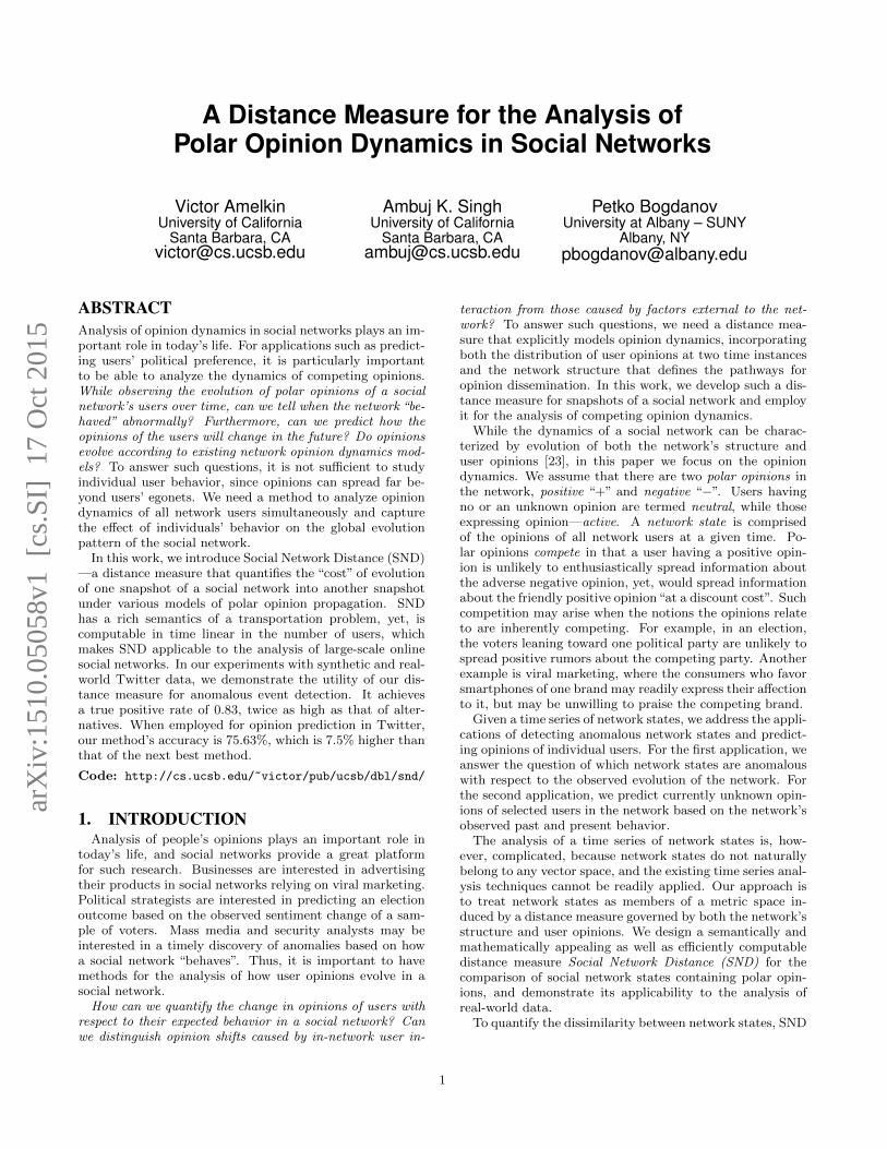
6.2 Detecting Anomalous Network StatesSynthetic Data: In a series of network states, we wantto detect which ones are anomalous. In particular, we areinterested in the anomalies which are hard to detect by ob-serving the summary of the social network (e.g., the numberof new activations). Thus, in experiments with syntheticdata, to simulate an anomaly, we change the values of Pnbrand Pext preserving their sum, thereby, affecting only qual-itatively the process of new users’ activation. In a series ofnetwork states, we compute the distances between the ad-jacent states, normalize these distances by the number ofactive users, and scale. Then, spikes in the resulting seriesof distances are considered anomalies.

A qualitative analysis of anomaly detection on syntheticdata is presented in Fig. 7. For each simulated anomaly,

Network state pair indexD

ista

nce

(sca

led)

0

0.2

0.4

0.6

0.8

1

Distance between adjacent network states

SND hamming walk-dist quad-form simulated anomaly

Figure 7: Anomaly detection on synthetic data. |V | = 20k,scale-free exponent γ = −2.3. A series of 40 network statesis generated using Pnbr = 0.12 and Pext = 0.01 for normaland Pnbr = 0.08 and Pext = 0.05 for anomalous networkstates’ generation.

SND produces a well noticeable spike, while other distancemeasures do not recognize such anomalies.

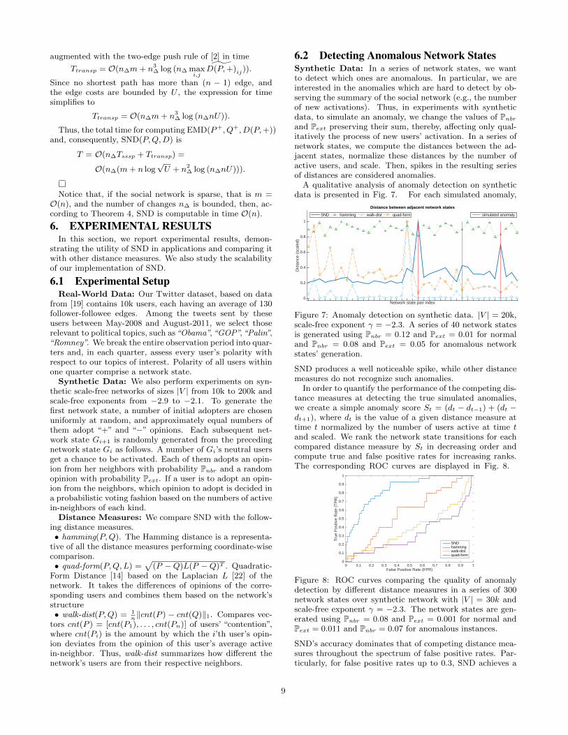
In order to quantify the performance of the competing dis-tance measures at detecting the true simulated anomalies,we create a simple anomaly score St = (dt − dt−1) + (dt −dt+1), where dt is the value of a given distance measure attime t normalized by the number of users active at time tand scaled. We rank the network state transitions for eachcompared distance measure by St in decreasing order andcompute true and false positive rates for increasing ranks.The corresponding ROC curves are displayed in Fig. 8.

0 0.1 0.2 0.3 0.4 0.5 0.6 0.7 0.8 0.9 1False Positive Rate (FPR)

0

0.1

0.2

0.3

0.4

0.5

0.6

0.7

0.8

0.9

1

Tru

e P

ositi

ve R

ate

(TP

R)

SNDhammingwalk-distquad-form

Figure 8: ROC curves comparing the quality of anomalydetection by different distance measures in a series of 300network states over synthetic network with |V | = 30k andscale-free exponent γ = −2.3. The network states are gen-erated using Pnbr = 0.08 and Pext = 0.001 for normal andPext = 0.011 and Pnbr = 0.07 for anomalous instances.

SND’s accuracy dominates that of competing distance mea-sures throughout the spectrum of false positive rates. Par-ticularly, for false positive rates up to 0.3, SND achieves a

9

true positive rate of 0.83, while the next best distance mea-sure (hamming) achieves only 0.4.Twitter Data: To obtain the ground truth for anomalydetection on our Twitter dataset, we collect“search interest”data from Google Trends3 and cross-check this data withAmerican Presidents4 log of important political events inthe US. The anomaly detection results for topic “Obama”are shown in Fig. 9.

05'0

8-11

'08

08'0

8-02

'09

11'0

8-05

'09

02'0

9-08

'09

05'0

9-11

'09

08'0

9-02

'10

11'0

9-05

'10

02'1

0-08

'10

05'1

0-11

'10

08'1

0-02

'11

11'1

0-05

'11

02'1

1-08

'11

Dis

tanc

e (s

cale

d)

0.2

0.4

0.6

0.8

1

1.2

1.4

Distance between adjacent network states (topic "Obama")

SNDhammingwalk-distquad-form

election

Economic Stimulus BillNobel Prize

"Obama Care"Tax plan

bin Laden

inauguration

anomaly interest

Figure 9: Anomaly detection on Twitter data (May’08-Aug’11) for topic “Obama”. The plots for distances betweennetwork states are accompanied by the plot showing GoogleTrends’ (scaled) interest in topic “Obama”. Network statesdetected to be anomalous by at least one distance measureare indicated with red vertical lines.

We can distinguish two types of network states and, hence,events based on SND’s behavior relatively to other distancemeasures. One type is the events corresponding to networkstates where SND agrees with other distance measures. Twoexamples are (i) the first anomaly – Barack Obama’s electionfor the President of the US, and (ii) bin Laden’s death beingthe last spike on the Google Trends curve (even though, alldistance measures noticeably increase their value during thelast quarter, we do not mark this quarter as anomalous, sincewe do not have the distance values for the next quarter.)These events are unlikely to have been perceived differentlyby the US users of Twitter and, hence, probably have notprovoked a polarized response.

The other type of events are those where SND noticeablydisagrees with other distance measures. For example, dur-ing quarters 05’09-11’09, the Economic Stimulus Bill hada highly polarized response in the House of Representa-tives5, with no Republican voting in its favor. Another suchanomaly takes place during quarters 02’10-08’10, when theAffordable Care Act (“Obama Care”) was introduced, andwhich was and still remains a very controversial topic. Thelatter can be seen from the House vote distribution6 andfrom the fact that, according to socialmention.com7, evenin October 2015, “Obama Care” is still perceived equallypositively and negatively in microblogs.

6.3 Predicting User OpinionsGiven a series of states of a social network we want to

predict the unknown opinions of the users in the currentnetwork state G0 based on the observed recent G−t (t ∈ N)and the (incomplete) current network states. For example,

3http://www.google.com/trends/explore

4http://www.american-presidents-history.com

5http://www.nytimes.com/2009/01/29/us/politics/29obama.html

6Democrats – 219 yeas, republicans – 212 nays (http://www.

healthreformvotes.org/congress/roll-call-votes/h165-111.2010)7http://socialmention.com/search?q=%22obama+care%22

if certain Twitter users have not tweeted (enough) in thecurrent quarter, we may want to predict the opinions ofthese users in the current quarter based on the observedopinions of all users of the network. We assume that duringthe periods corresponding to the observed recent networkstates G−t, the social network evolved “smoothly”, that is,the recent states can predict the current state. Under thisassumption, we use a distance measure to compute the dis-tances dist(G−t, G−t+1) between the adjacent past networkstates, then, extrapolate the obtained series to estimate thedistance d∗ from the most recent G−1 to the yet unknowncomplete current network state. Then, we assign differentopinions to the target users in the current network state,trying to make the distance dist(G−1, G

∗0) from the most

recent to the modified current network state as close to es-timate d∗ as possible. The search for the best assignment ofopinions to the target users is randomized — the number ofthe uniformly randomly generated opinion assignments forall target users is considerably lower than the total num-ber of possible assignments (we use 100 random opinion as-signments in each experiment). In each experiment, we uni-formly randomly select 20 active users – with approximatelyequal number of positive and negative users – in the currentnetwork state, predict their opinions and measure the pre-diction accuracy. This procedure is repeated 10 times, andmean accuracies and standard deviations are reported.

The predictions are made using the above distance-basedmethod with SND as well as other distance measures. To putthe prediction performance of these methods in context, weadd into comparison two non-distance-based methods – onebasic, and one state-of-the-art – that make predictions basedon the known quantified opinions of the users and the net-work’s structure. One such method, nhood-voting, derivesthe opinion of each target user based on the opinions of thisuser’s active in-neighbors in a probabilistic voting fashion,or selects it uniformly randomly in the absence of active in-neighbors. Another method, community-lp [9, IV.B] detectscommunities in the network via label propagation and, then,predicts user opinions based on these users’ membership inthe discovered communities.

We experiment on both synthetic and real-world data.For synthetic data, we generate a scale-free network withn = 10k users and scale-free exponent γ = −2.5. A series ofnetwork states is generated using the same algorithm as inthe case with anomaly detection, with probabilities of opin-ion adoption from the neighborhood and from the “externalsource” ranging between 0.001 and 0.2. The number of ini-tial adopters in the first network state is 800. We use 3 mostrecent network states to estimate the distance from the mostrecent to the incomplete current network state.

Results for opinion prediction are summarized in Table 1.There are three important observations:• Firstly, among the distance-based methods, the one that

uses SND always performs best, with an average predic-tion accuracy of 74-75% and a consistently low standarddeviation. This suggests that SND captures more opiniondynamics-specific information than the other distance mea-sures, and should be preferred, particularly, when such sim-ple statistics as the rate of new user activation are uninfor-mative.• Secondly, SND-based prediction method works consider-

ably better than method nhood-voting that bases the opin-ion prediction for each user on the opinions of the user’s

10

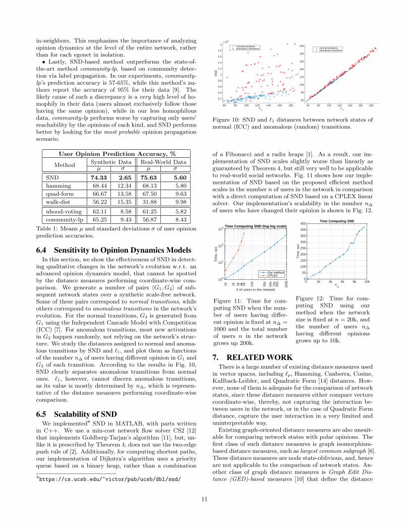
in-neighbors. This emphasizes the importance of analyzingopinion dynamics at the level of the entire network, ratherthan for each egonet in isolation.• Lastly, SND-based method outperforms the state-of-

the-art method community-lp, based on community detec-tion via label propagation. In our experiments, community-lp’s prediction accuracy is 57-65%, while this method’s au-thors report the accuracy of 95% for their data [9]. Thelikely cause of such a discrepancy is a very high level of ho-mophily in their data (users almost exclusively follow thosehaving the same opinion), while in our less homophilousdata, community-lp performs worse by capturing only users’reachability by the opinions of each kind, and SND performsbetter by looking for the most probable opinion propagationscenario.

User Opinion Prediction Accuracy, %

Method Synthetic Data Real-World Dataµ σ µ σ

SND 74.33 2.65 75.63 5.60

hamming 68.44 12.34 68.13 5.80

quad-form 66.67 13.58 67.50 9.63

walk-dist 56.22 15.35 31.88 9.98

nhood-voting 62.11 8.58 61.25 5.82

community-lp 65.25 9.43 56.87 8.43

Table 1: Means µ and standard deviations σ of user opinionprediction accuracies.

6.4 Sensitivity to Opinion Dynamics ModelsIn this section, we show the effectiveness of SND in detect-

ing qualitative changes in the network’s evolution w.r.t. anadvanced opinion dynamics model, that cannot be spottedby the distance measures performing coordinate-wise com-parison. We generate a number of pairs 〈G1, G2〉 of sub-sequent network states over a synthetic scale-free network.Some of these pairs correspond to normal transitions, whileothers correspond to anomalous transitions in the network’sevolution. For the normal transitions, G2 is generated fromG1 using the Independent Cascade Model with Competition(ICC) [7]. For anomalous transitions, most new activationsin G2 happen randomly, not relying on the network’s struc-ture. We study the distances assigned to normal and anoma-lous transitions by SND and `1, and plot them as functionsof the number n∆ of users having different opinion in G1 andG2 of each transition. According to the results in Fig. 10,SND clearly separates anomalous transitions from normalones. `1, however, cannot discern anomalous transitions,as its value is mostly determined by n∆, which is represen-tative of the distance measures performing coordinate-wisecomparison.

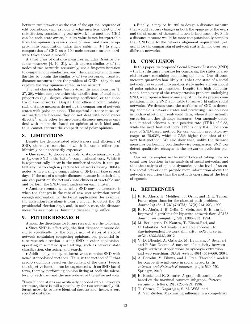
6.5 Scalability of SNDWe implemented8 SND in MATLAB, with parts written

in C++. We use a min-cost network flow solver CS2 [12]that implements Goldberg-Tarjan’s algorithm [11], but, un-like it is prescribed by Theorem 4, does not use the two-edgepush rule of [2]. Additionally, for computing shortest paths,our implementation of Dijkstra’s algorithm uses a priorityqueue based on a binary heap, rather than a combination

8https://cs.ucsb.edu/~victor/pub/ucsb/dbl/snd/

n"

60 80 100 120 140 160 180

SN

D

#104

0.2

0.4

0.6

0.8

1

1.2

1.4

1.6

1.8

2normal transitionsanomalous transitions

n"

60 80 100 120 140 160 180

l 1

60

80

100

120

140

160

180

200normal transitionsanomalous transitions

Figure 10: SND and `1 distances between network states ofnormal (ICC) and anomalous (random) transitions.

of a Fibonacci and a radix heaps [1]. As a result, our im-plementation of SND scales slightly worse than linearly asguaranteed by Theorem 4, but still very well to be applicableto real-world social networks. Fig. 11 shows how our imple-mentation of SND based on the proposed efficient methodscales in the number n of users in the network in comparisonwith a direct computation of SND based on a CPLEX linearsolver. Our implementation’s scalability in the number n∆

of users who have changed their opinion is shown in Fig. 12.

# of users in the network

1k

2k

3k

4k

5k

10k

30k

50k

70k

90k

200k

Tim

e, s

ec

100

101

102

103 Time Computing SND (log-log scale)

Our methodCPLEX

Figure 11: Time for com-puting SND when the num-ber of users having differ-ent opinion is fixed at n∆ =1000 and the total numberof users n in the networkgrows up 200k.

n"

0 2k 4k 6k 8k 10k

Tim

e, s

ec

0

50

100

150

200

250

300

350

400

450Time Computing SND

Figure 12: Time for com-puting SND using ourmethod when the networksize is fixed at n = 20k, andthe number of users n∆

having different opinionsgrows up to 10k.

7. RELATED WORKThere is a large number of existing distance measures used

in vector spaces, including `p, Hamming, Canberra, Cosine,Kullback-Leibler, and Quadratic Form [14] distances. How-ever, none of them is adequate for the comparison of networkstates, since these distance measures either compare vectorscoordinate-wise, thereby, not capturing the interaction be-tween users in the network, or in the case of Quadratic Formdistance, capture the user interaction in a very limited anduninterpretable way.

Existing graph-oriented distance measures are also unsuit-able for comparing network states with polar opinions. Thefirst class of such distance measures is graph isomorphism-based distance measures, such as largest common subgraph [6].These distance measures are node state-oblivious, and, henceare not applicable to the comparison of network states. An-other class of graph distance measures is Graph Edit Dis-tance (GED)-based measures [10] that define the distance

11

between two networks as the cost of the optimal sequence ofedit operations, such as node or edge insertion, deletion, orsubstitution, transforming one network into another. GEDcan be node state-aware, but its value is not interpretablefrom the opinion dynamics point of view, and even its ap-proximate computation takes time cubic in |V | (a singlecomputation of GED on a 10k-node network on our hard-ware takes about a month).

A third class of distance measures includes iterative dis-tance measures [4, 16, 21], which express similarity of thenodes of two networks recursively, use a fix-point iterationto compute node similarities, and, then, aggregate node sim-ilarities to obtain the similarity of two networks. Iterativedistance measures share the problem of GED – they do notcapture the way opinions spread in the network.

The last class includes feature-based distance measures [3,27, 29], which compare either the distributions of local nodeproperties (e.g., degree, clustering coefficient) or the spec-tra of two networks. Despite their efficient computability,such distance measures do not fit the comparison of networkstates with polar opinions. The spectral distance measuresare inadequate because they do not deal with node statesdirectly9, while other feature-based distance measures onlydeal with summaries based on opinion of each kind and,thus, cannot capture the competition of polar opinions.

8. LIMITATIONSDespite the demonstrated effectiveness and efficiency of

SND, there are scenarios in which its use is either pro-hibitively or unnecessarily expensive.• One reason to choose a simpler distance measure, such

as `p, over SND is the latter’s computational cost. While itis asymptotically linear in the number of nodes, it can, po-tentially, be too high in practice for networks having 100M+nodes, where a single computation of SND can take severaldays. If the use of a simpler distance measure is undesirable,one can partition the network into clusters of tractable sizeand perform the SND-based analysis on each cluster.• Another scenario when using SND may be excessive is

when the changes in the rate of new user activation revealenough information for the target application (for example,the activation rate alone is clearly enough to detect the USpresidential election day), and, in such a case, the distancemeasures as simple as Hamming distance may suffice.

9. FUTURE RESEARCHAmong the directions for future research are the following.• Since SND is, effectively, the first distance measure de-

signed specifically for the comparison of states of a socialnetwork containing competing opinions, one potential fu-ture research direction is using SND in other applicationsoperating in a metric space setting, such as network stateclassification, clustering, and search.• Additionally, it may be lucrative to combine SND with

non-distance-based methods. Thus, in the method of [9] thatpredicts opinions based on the content of the users’ tweets,the objective function can be augmented with an SND-basedterm, thereby, performing opinion fitting at both the micro-level of each user and the macro-level of the entire network.

9Even if node states are artificially encoded into a network’sstructure, there is still a possibility for two structurally dif-ferent networks to have identical spectra and, hence, a zerospectral distance.

• Finally, it may be fruitful to design a distance measurethat would capture changes in both the opinions of the usersand the structure of the social network simultaneously. Sucha distance measure would be more computationally complexthan SND due to the network alignment requirement, yet,useful for the comparison of network states defined over verydifferent networks.

10. CONCLUSIONIn this paper, we proposed Social Network Distance (SND)

– the first distance measure for comparing the states of a so-cial network containing competing opinions. Our distancemeasure quantifies how likely it is that one state of a socialnetwork has evolved into another state under a given modelof polar opinion propagation. Despite the high computa-tional complexity of the transportation problem underlyingSND, we propose a linear-time algorithm for its precise com-putation, making SND applicable to real-world online socialnetworks. We demonstrate the usefulness of SND in detect-ing anomalous network states and predicting user opinionsin both synthetic and real-world data, where it consistentlyoutperforms other distance measures. Our anomaly detec-tion method achieves a true positive rate (TPR) of 0.83,while the next best method’s TPR is only 0.4. The accu-racy of SND-based method for user opinion prediction av-erages at 75.63%, which is 7.5% higher than that of thenext best method. We also show that, unlike the distancemeasures performing coordinate-wise comparison, SND candetect qualitative changes in the network’s evolution pat-tern.

Our results emphasize the importance of taking into ac-count user locations in the analysis of social networks, andthat the analysis of opinion dynamics at the level of an en-tire social network can provide more information about thenetwork’s evolution than the methods operating at the levelof egonets.

11. REFERENCES[1] R. K. Ahuja, K. Mehlhorn, J. Orlin, and R. E. Tarjan.

Faster algorithms for the shortest path problem.Journal of the ACM (JACM), 37(2):213–223, 1990.

[2] R. K. Ahuja, J. B. Orlin, C. Stein, and R. E. Tarjan.Improved algorithms for bipartite network flow. SIAMJournal on Computing, 23(5):906–933, 1994.

[3] M. Berlingerio, D. Koutra, T. Eliassi-Rad, andC. Faloutsos. NetSimile: a scalable approach tosize-independent network similarity. arXiv preprintarXiv:1209.2684, 2012.

[4] V. D. Blondel, A. Gajardo, M. Heymans, P. Senellart,and P. Van Dooren. A measure of similarity betweengraph vertices: Applications to synonym extractionand web searching. SIAM review, 46(4):647–666, 2004.

[5] A. Borodin, Y. Filmus, and J. Oren. Threshold modelsfor competitive influence in social networks. InInternet and Network Economics, pages 539–550.Springer, 2010.

[6] H. Bunke and K. Shearer. A graph distance metricbased on the maximal common subgraph. Patternrecognition letters, 19(3):255–259, 1998.

[7] T. Carnes, C. Nagarajan, S. M. Wild, andA. Van Zuylen. Maximizing influence in a competitive

12

social network: a follower’s perspective. EC, pages351–360, 2007.

[8] K. L. Clarkson. Nearest-neighbor searching and metricspace dimensions. Nearest-neighbor methods forlearning and vision: theory and practice, pages 15–59,2006.

[9] M. D. Conover, B. Goncalves, J. Ratkiewicz,A. Flammini, and F. Menczer. Predicting the politicalalignment of Twitter users. In SocialCom. IEEE, 2011.

[10] X. Gao, B. Xiao, D. Tao, and X. Li. A survey ofGraph Edit Distance. Pattern Analysis andapplications, 13(1):113–129, 2010.

[11] A. Goldberg and R. Tarjan. Solving minimum-costflow problems by successive approximation. InProceedings of the nineteenth annual ACM symposiumon Theory of computing, pages 7–18. ACM, 1987.

[12] A. V. Goldberg. An efficient implementation of ascaling minimum-cost flow algorithm. Journal ofalgorithms, 22(1):1–29, 1997.

[13] A. Goyal, F. Bonchi, and L. V. Lakshmanan. Learninginfluence probabilities in social networks. WSDM,pages 241–250, 2010.

[14] J. Hafner, H. S. Sawhney, W. Equitz, M. Flickner, andW. Niblack. Efficient color histogram indexing forquadratic form distance functions. Pattern Analysisand Machine Intelligence, IEEE Transactions on,17(7):729–736, 1995.

[15] D. B. Johnson. Efficient algorithms for shortest pathsin sparse networks. Journal of the ACM (JACM),24(1):1–13, 1977.

[16] E. Leicht, P. Holme, and M. Newman. Vertexsimilarity in networks. Physical Review E,73(2):026120, 2006.

[17] L. Li, M. Ma, P. Lei, X. Wang, and X. Chen. A linearapproximate algorithm for Earth Mover’s Distancewith thresholded ground distance. MathematicalProblems in Engineering, 2014.

[18] V. Ljosa, A. Bhattacharya, and A. K. Singh. Indexingspatially sensitive distance measures usingmulti-resolution lower bounds. EDBT, pages 865–883,2006.

[19] K. Macropol, P. Bogdanov, A. K. Singh, L. Petzold,and X. Yan. I act, therefore I judge: Networksentiment dynamics based on user activity change.ACM ASONAM, pages 396–402, 2013.

[20] A. McGregor and D. Stubbs. Sketching earth-moverdistance on graph metrics. In Approximation,Randomization, and Combinatorial Optimization.Algorithms and Techniques, pages 274–286. Springer,2013.

[21] S. Melnik, H. Garcia-Molina, and E. Rahm. Similarityflooding: A versatile graph matching algorithm and itsapplication to schema matching. In Data Engineering,2002. Proceedings., pages 117–128. IEEE, 2002.

[22] R. Merris. Laplacian matrices of graphs: a survey.Linear algebra and its applications, 197:143–176, 1994.

[23] S. A. Myers and J. Leskovec. The bursty dynamics ofthe Twitter information network. In Proceedings of the23rd international conference on World wide web,pages 913–924. ACM, 2014.

[24] O. Pele and M. Werman. A linear time histogram

metric for improved SIFT matching. In ComputerVision–ECCV 2008, pages 495–508. Springer, 2008.

[25] Y. Rubner, C. Tomasi, and L. J. Guibas. The EarthMover’s Distance as a metric for image retrieval.International Journal of Computer Vision,40(2):99–121, 2000.

[26] Y. Tang, U. Leong Hou, Y. Cai, N. Mamoulis, andR. Cheng. Earth Mover’s Distance based similaritysearch at scale. Proceedings of the VLDB Endowment,7(4):313–324, 2013.

[27] R. C. Wilson, E. R. Hancock, and B. Luo. Patternvectors from algebraic graph theory. Pattern Analysisand Machine Intelligence, IEEE Transactions on,27(7):1112–1124, 2005.

[28] E. Yildiz, D. Acemoglu, A. E. Ozdaglar, A. Saberi,and A. Scaglione. Discrete opinion dynamics withstubborn agents. Available at SSRN 1744113, 2011.

[29] P. Zhu and R. C. Wilson. A study of graph spectra forcomparing graphs. In BMVC, 2005.

13