THE FUTURE OF INDIAN COTTON SUPPLY AND DEMAND:

IMPLICATIONS FOR THE U.S. COTTON INDUSTRY

by

JAGADANAND CHAUDHARY, M.Sc.

A DISSERTATION

IN

AGRICULTURAL AND APPLIED ECONOMICS

Submitted to the Graduate Faculty of Texas Tech University in

Partial Fulfillment of the Requirements for

the Degree of

DOCTOR OF PHILOSOPHY

Approved

Samarendu Mohanty Co-Chairperson of the Committee

Sukant Misra Co-Chairperson of the Committee

Jaime Malaga

Robert Paige

Accepted

John Borrelli

Dean of the Graduate School

AUGUST, 2005

ACKNOWLEDGEMENTS

I would like to express my gratitude to my committee co-chairmen Dr.

Samarendu Mohanty and Dr. Sukant Misra for their advice, guidance and patience in the

completion of this work. I would also like to thank my committee members Dr. Jaime

Malaga and Dr. Robert Paige for their suggestions and time on this project. In addition I

want to thank Dr. Don E. Ethridge for the financial assistance provided by him. I wish to

express my appreciation to Dr. Eduardo Segarra for his advice, encouragement and help

throughout the study period. I would also like to thank Dr. Suwen Pan for his expertise

and time on this project. I am grateful to the faculty, staff and colleagues of Agricultural

and Applied Economics Department for their kind support.

Finally, I appreciate my family for their support and sacrifices throughout the

study period. Without their support, I could not have been able to complete the work.

ii

TABLE OF CONTENTS

ACKNOWLEDGEMENTS ii

LIST OF TABLES v LIST OF FIGURES vii

I. INTRODUCTION 1

1.1. General Problem 6 1.2. Specific Problem 8 1.3. General Objective 9 1.4. Specific Objectives 9

II. LITERATURE REVIEW 11

2.1. Partial Equilibrium Cotton Models 11

2.2. Studies Related to Cotton Supply Estimation 20 2.3. Studies Related to Cotton Demand Estimation 23 2.4. Studies Examining Competitiveness of Cotton 30 2.5. Summary 32

III. CONCEPTUAL FRAMEWORK 34

3.1. Supply Response 38 3.1.1. Cotton Acreage and Yield Response 41 3.1.2. Man-made Fiber Production Response 44 3.2. Demand Specifications 46 3.2.1. Demand for Textile Products 49 3.2.2. Cotton Demand 50 3.3. Competitiveness of U.S. Cotton 57

3.3.1. Cotton Import Demand 59 3.4. Summary 59

IV. METHODS AND PROCEDURES 61 4.1. Model Specification 64 4.1.1. Fiber Supply Estimation 64 4.1.1.1. Cotton Supply Model 64 4.1.1.2. Man-made Fiber Supply Model 66 4.1.2. Fiber Demand Estimation 67

iii

4.1.3. Cotton Ending Stocks and Trade Equations 69 4.1.4. Market Clearing Condition 70 4.2. Policy Simulations 72 4.3. Competitiveness of U.S. Cotton 73 4.4. Model Validation 74 4.5. Data Requirements 78 4.6. Summary 80 V. RESULTS AND DISCUSSIONS 82 5.1. Fiber Supply Model 82 5.1.1. Cotton Acreage Model 82 5.1.2. Cotton Yield Model 87 5.1.3. Man-made Fiber Supply Model 90 5.2. Fiber Demand Models 92 5.2.1. Per Capita Textile Consumption 92 5.2.2. Fiber Demand 94 5.3. Fiber Trade and Cotton Ending Stocks Equations 99 5.4. Model Validation 105 5.5. Policy Simulation 107 5.5.1. Baseline Projections 109 5.5.2. Simulation Results 113 5.6. Competitiveness of U.S. Cotton 124

VI. SUMMARY AND CONCLUSIONS 132

6.1. Summary of the Results 132 6.2. Conclusions 138 6.3. Limitations of the Study 140 REFERENCES 142 APPENDIX: List of Variables and their Unit of Measurement 145

iv

LIST OF TABLES

5.1. Regression Results of Indian Regional Cotton Acreage Models 83 5.2. Elasticities of Indian Regional Cotton Acreage Model at mean level 86

5.3: Regression Results of Indian Regional Cotton Yield Models 88

5.4. Regression Results of Manmade Fiber Capacity and Utilization 91

5.5. Regression Results of Per Capita Textile Consumption 93

5.6. Regression Results of Fiber Demand System 96

5.7. Estimated Uncompensated Fiber Price and Income Elasticities 97

5.8. Estimated Compensated Fibers Price Elasticities 98

5.9. Regression Results of Cotton Trade Equations 100

5.10. Regression Results of Man-made Fiber Net Trade 103

5.11. Regression Results of Cotton Ending Stocks 104

5.12. Model Validation Statistics 106 5.13. Summary of Baseline Projections for Fiber Demand, Cotton Price, Polyester Price, Fiber Production, and Fiber Trade in India, 2004/05-2014/15. 112 5.14. Effects of MFA Quota Elimination on Indian Fiber Consumption and Domestic Fiber Prices 115 5.15. Effects of MFA Quota Elimination on Indian Cotton Area 116 5.16. Effects of MFA Quota Elimination on Indian Cotton Yield 117 5.17. Effects of MFA Quota Elimination on Indian Fiber Supply 118 5.18. Effects of MFA Quota Elimination on Fiber Trade and World Price 119 5.19. Wald Chi-Square Statistic test for the Results of Unrestricted and Restricted Models 125

v

5.20. Estimated Coefficients of the Restricted AIDS model 126 5.21. Estimated Uncompensated Elasticities of the Restricted Model 127 5.22. Estimated Compensated Elasticities of the Restricted Model 129

vi

LIST OF FIGURES

1.1. Market Shares of the United States in the Indian Cotton Market 2 3.1. Impacts of MFA Quota Elimination on World Cotton and Indian Textile Markets 35 4.1. Schematic Representation of the Indian Fiber Model 62 5.1. Baseline Projections for Textile Consumption in India 110 5.2. Baseline Projections of the Domestic Fiber Prices 111 5.3. Baseline Fiber Net Trade Projections 114 5.4. Indian Man-made Fiber Net Trade Projections (Baseline vs. Scenario) 122

vii

CHAPTER I

INTRODUCTION

India has the largest cotton-producing area in the world, accounting for 25 percent

of the world acreage, but contributes only 14 percent to the world production. China and

the United States produce more cotton than India with substantially less area. In the last

decade (between 1993/94 and 2002/03), Indian cotton production has increased by only 8

percent (average annual growth of less than one percent). Consumption in India,

however, has grown by around 35 percent during the same period, primarily fueled by

rapid expansion in textile consumption and exports. Currently, India is the second largest

textile producer in the world after China, accounting for about 15 percent of world

production, with export exceeding 12 billion U.S. dollars.

Disparity of growth in cotton production and consumption in the last decade has

transformed India from a net exporter to a net importer of cotton. As recently as 1996,

India exported more than 4 percent of world's cotton. Since 1999, India has instead

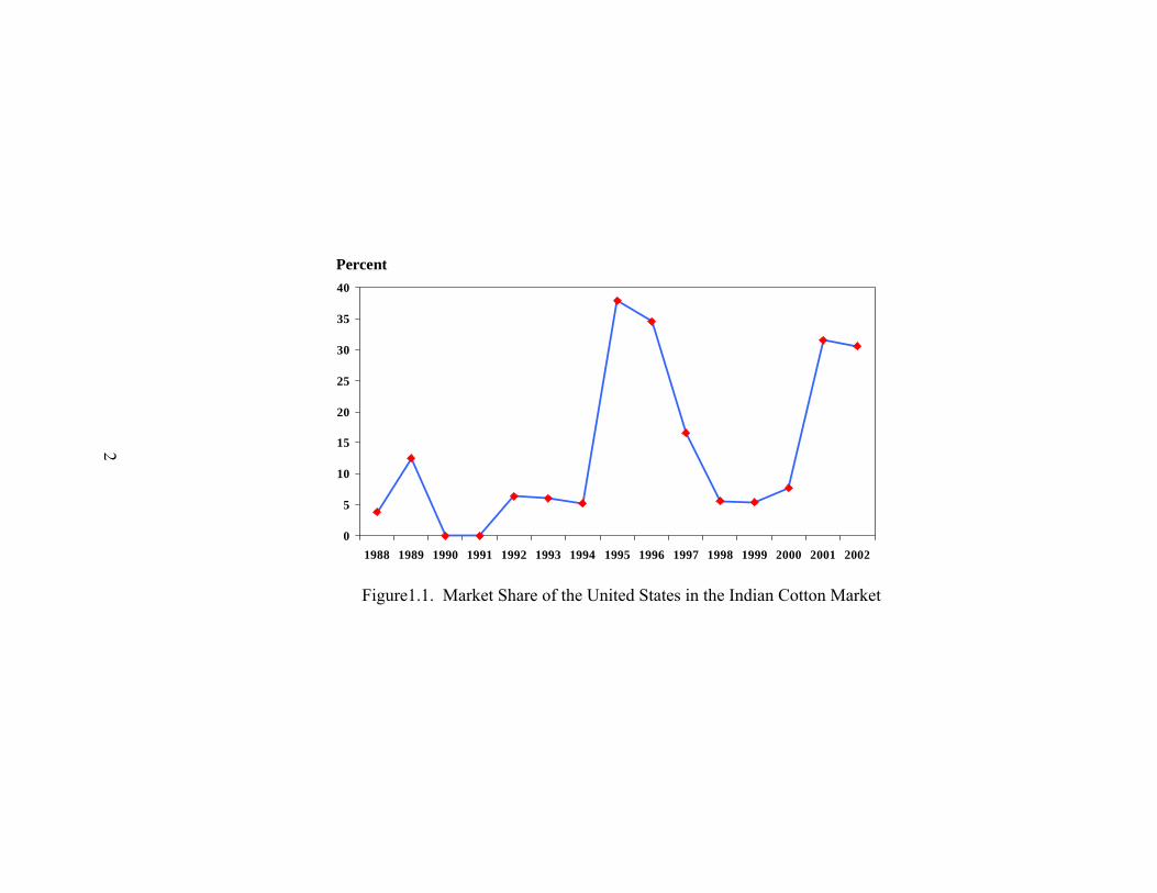
accounted for about 6 percent of world imports with the record amount of 480 thousand

metric tons in 1999/00. The U.S. share of India’s cotton market, however, remains

highly unstable. For example, the U.S. share of the total Indian cotton imports has

decreased from 30 percent in 1995 and 1996 to about 5 percent in 2000 (Figure 1.1).

Since then, the U.S. exports to India have recovered accounting for around 30 percent of

the market share in 2001 and 2002. While the U.S. has emerged as an important supplier

over the last two seasons, prices will have to remain competitive in order to offset the

1

0

5

10

15

20

25

30

35

40

1988 1989 1990 1991 1992 1993 1994 1995 1996 1997 1998 1999 2000 2001 2002

Percent

2

Figure1.1. Market Share of the United States in the Indian Cotton Market

lower freight and shorter delivery periods offered to Indian buyers by Egypt, West

Africa, and Australia.

India’s reemergence as a major cotton importer has occurred mainly because of

external and internal constraints. The external constraint was the Multi-Fiber

Arrangement (MFA), which provided a framework under which developed countries

abided by a quota on the export of yarn, textiles and apparel from the developing

countries. The history of quantitative restrictions goes back to 1930’s when it was first

imposed by developed countries against the increasingly competitive Japanese cotton

textile industries. Later on, it expanded into a system of voluntary export restrictions on

almost all significant suppliers of textiles or clothing. The Long Term Cotton

Arrangement governed the period 1962-1973 and the MFA was established for the period

1974-1994. Gradually, many importing countries (Sweden, Switzerland, and Australia

among them) left the MFA. By 1994, the MFA included only four importers (the US, the

EU, Canada, and Norway) and some 30 developing exporting countries with a total of

1,300 bilateral quotas on textiles and clothing.

Quotas are applied typically on a bilateral basis, under the threat of unilateral

restraints to be imposed by the importing country. The quotas are determined through

bilateral negotiations and are specific to particular product categories, as defined by fiber

and by function. The MFA allowed for discrimination not only against specific fibers

and products, but also among exporting countries. The quotas for apparel exports were

announced for three-year periods and were subject to specific criteria.

The MFA system is a departure from two of the most fundamental principles of

3

the multilateral trading system. These are: (i) the ban on quantitative restrictions, and (ii)

the prohibition of discrimination between suppliers of textiles and apparels. In the

Uruguay Round of the General Agreement on Tariffs and Trade (GATT), the Agreement

on Textiles and Clothing (ATC) negotiated the phase-out of the MFA over a ten-year

period beginning in 1995. The ATC stipulated liberalization to occur in four stages and

in two forms: (i.) integration, and (ii.) an acceleration of quota growth. At the end of

fourth and the final stage, i.e., by January 1, 2005, all bilateral quotas between developing

exporters and developed importers ceased to exist.

Internal constraints included a mandate to sustain the small-scale traditional

handloom sector, export constraints on yarn, government fixing of cotton ginning and

pressing fees, subsidization of raw cotton production, and an overvalued exchange rate.

These policies have generally kept domestic cotton producer prices well below the world

prices. Cotton production policies in India historically have been oriented towards

promoting and supporting the textile industry. Government of India (GOI) announces

minimum support prices for cotton every year and the Cotton Corporation of India (CCI),

a government-owned organization, sets the minimum support prices for each cotton

variety. The minimum support price is fixed by the Textile Commissioner for the Fair

Average Quality (FAQ) grade of each variety of seed cotton on the basis of

recommendations from the Commission for Agricultural Costs and Prices (CACP). The

CCI is responsible for procuring cotton from the free market to support these prices. In

addition, the GOI also heavily subsidizes fertilizers, electricity, and water to producers.

This is illustrated by the increase in the fertilizer subsidy from 60 billion rupees in

4

1992/93 to 140 billion in 2001/02 (Mohanty et al., 2002). The food and input subsidies

have accounted for approximately 5 percent of all government expenditures in 2002,

exceeding more than $12 billion dollars (Landes, 2004).

The GOI also intervenes in the cotton market from storage, movement and credit

controls, to the fixing of ginning fees, and restrictions on the scale of operations in the

ginning sector. On the trade front, the GOI controls cotton exports to provide cheap

cotton to the textile mills by announcing an annual export quota. Historically, the quota

has ranged from 8,000 Metric Tons (MT) to 303,600 MT depending on the local supply

and demand situation (World Bank, 1999).

India’s internally-imposed constraints extend across its entire development policy,

which until the 1990’s looked to internal markets and investment, spurning the

opportunities for transformation offered by foreign investment and competition. In 1991,

the GOI initiated significant economic reforms and structural adjustment polices. The

policies were targeted primarily at industry and the international trade regime, affecting

agriculture only indirectly through reductions in input subsidies. More recently, the GOI

announced its intent to reform the cotton and textile sector, but there were no specifics as

to what would be done or when. These reforms also included research, education,

irrigation development programs, an institutional framework for land ownership, and

plans to improve technology (Worden and Heitzman, 1999). In addition to these

unilateral reforms, India, as a member of World Trade Organization (WTO), is

committed to open its agriculture market to the world market. However, in the early

years of GATT, India under Article XVIII-B imposed quantitative restrictions on imports

5

because of problems in the Balance of Payments (BOP) account. Since 1997, India has

been removing many import licensing and quota restrictions and replacing them with

high tariffs as part of its WTO commitments (Gulati and Kelly, 2000).

Although the GOI, under pressure from trading partners, has removed quantitative

restrictions such as licensing and quota restrictions on imports of most agricultural

products, higher tariffs and other non-tariff barriers continue to shield the farm sector.

For example, wheat, cotton, and corn, which formerly carried no duty, are now subject to

tariffs, while the tariffs on edible oils, wine, poultry, and sugar have been sharply

increased (USDA, 2001).

1.1. General Problem

The effects of India’s unilateral liberalization on its cotton industry have been

significant. As the invigoration (revitalization) of textile exports drove cotton

consumption well above the pace of the rest of the world, India’s share of world

consumption has increased from 10 percent in 1990/91 to 15 percent in 1999/2000.

Virtually, all of the 50 percent increase in India’s cotton consumption to date has been

met through increased production. India’s cotton area was already the world’s largest by

a significant margin in 1990, but by 1997 India’s cotton area has increased by another 2

million hectares; with increase occurring in each of India’s three main growing regions1.

1 The regions include: (i) the northern zone (Haryana, Punjab, and Rajasthan); (ii)

the central zone (Maharashtra, Gujarat, and Madhya Pradesh); and (iii) the southern zone (Karnataka, Tamil Nadu and Andhra Pradesh). The northern region primarily grows short and medium staple cotton while the southern states primarily grow long staples. The central zone grows mostly medium and long staples cotton (Mohanty, et al., 2002).

6

Even with the increase in area and yield, India has emerged as a growing net importer of

cotton in recent years, and it is unclear how successfully India’s cotton sector will keep

pace with its burgeoning textile industry.

In the next few years, state interventions will be eliminated, and the external trade

constraints originally imposed under the MFA have already been eliminated.

Consequently, textiles and apparel were incorporated into the WTO structure that governs

world trade in general. As the world moves into the post-MFA era, a number of

questions arise about how the various segments of India’s textile industry will be

impacted, given that global competitors including China, Pakistan, and Southeast Asia

would no longer be constrained by quotas. India is also in the process of removing its

own import restrictions in order to meet its WTO obligations, which would likely further

impact cotton and textile production and trade patterns in both India and the rest of the

world.

In addition, India itself is a growing market for textile consumption. Following

the liberalization of 1991, India’s one billion consumers have increased their purchase of

apparel and textiles produced both domestically and abroad, with increasing implications

for the world market.

The overall picture of the textile and apparel sectors in India is one of great

potential with many unknowns. This potential is particularly important in light of the

liberalization in textiles and apparel trade foreseen under the Uruguay Round agreement

of the GATT, as well as ambitious export-led growth and liberalization programs

7

undertaken by the Indian Government since 1991 (Bhide et al., 1996). Full

implementation of the Uruguay Round Agreement and recent developments in the global

economy will also expose India’s textile and clothing sectors to more intense

competition, both at home from synthetics, and abroad from other major exporters such

as China. However, India has launched a series of initiatives such as further

liberalization of foreign investment restrictions on textiles, easy credit availability to

upgrade textile facilities, and the launch of a cotton technology initiative to respond to

upcoming challenges and opportunities. The ability of the cotton industry in India to

keep pace with changes in the textile industry will determine whether India would once

again become an important raw cotton exporter, or would remain a major source of world

import demand.

1.2. Specific Problem

Many studies project that India will be a major beneficiary of MFA textile quota

eliminations, with textile exports expanding by as much as 25 percent. In addition,

domestic textile consumption is also expected to increase rapidly in the future insofar as

the International Monetary Fund (IMF) and the World Bank project the Indian economy

to grow at 6-8 percent annually in the medium-term. The projected strong growth in

textile exports and domestic consumption would lead to the expansion of mill demand for

cotton, necessitating an increase in cotton production at a much faster pace than the

historical rate of less than one percent annually. Since cotton acreage is unlikely to

expand in the future, production growth will have to come through yield improvements.

8

Very few studies have examined the future of the Indian cotton market under the

scenario of MFA quota elimination and its effects on the world fiber market. However,

these studies have either failed to take into account substitutability between cotton and

man-made fibers, or appropriate linkage between cotton and textiles, thus producing

incomplete assessment of the elimination of MFA quota on the Indian cotton market and

the world fiber market. More specifically, a clear understanding of the effects of MFA

quota elimination on India’s cotton and apparel trade, and the subsequent competitiveness

of the U.S. cotton in the Indian market is still lacking.

1.3. General Objective

The general objective of this study is to analyze the demand for and the supply of

cotton in India in the Post-MFA era and its effects on the world fiber market, including

the United States.

1.4. Specific Objectives

The specific objectives are to:

1. Develop an empirical framework that incorporates regional supply response,

substitutability between cotton and man-made fibers, and appropriate linkage

between cotton and textile sectors to quantify demand, supply, and prices of

cotton and manmade fibers in India.

2. Assess the impacts of MFA textile quota elimination on the Indian and world

cotton market.

9

3. Identify factors influencing the competitiveness of U.S. cotton in the Indian

market.

10

CHAPTER II

LITERATURE REVIEW

This chapter reviews previous studies in the areas of cotton demand and supply

and is divided into four sections. The first section deals with the estimation of demand

and supply of cotton in a partial equilibrium framework. Studies related to cotton

demand estimation are dealt with in the next section, followed by crop supply response,

and competitiveness of U.S. cotton.

2.1. Partial Equilibrium Cotton Models

Hitchings (1984) developed an integrated supply-demand model in India to

analyze various policy issues relating to the cotton industry. The model consisted of

three stochastic equations – one for supply of lint, another for mill consumption of lint,

and a third for cotton textile consumption, as well as two identities to account for

adjusted trade and utilization balance, for cotton and for cotton textiles.

Cotton lint production was specified as a function of the lagged real lint and food

grain price indices, and the lagged proportion of cotton area under irrigation. Cotton mill

consumption was specified as the function of current and lagged real lint prices, lagged

real cotton textile price, and a time trend. Cotton textile consumption was dependent on

real textile prices and income. The difference between cotton production and lint

consumption captures the changes in the cotton ending stocks and net trade. Similarly,

the difference between cotton textile production (cotton mill consumption converted to a

11

cloth equivalent) and cotton textile consumption represents the cotton textile net trade

and the change in the ending stocks. The five-equation simultaneous model included lint

production, mill consumption of lint, textile consumption, the real lint price index, and

the real textile price index as the five current endogenous variables. The other nine non-

stochastic variables are exogenous, lagged endogenous, or constant and trend variables.

The elasticities of the structural form were derived from the reduced-form

coefficients. The production elasticities with respect to lagged real lint price, lagged real

food grain price, and lagged irrigation proportion were estimated to be 0.074, -0.567, and

0.421, respectively. Elasticities of cotton mill demand with respect to the lint and textile

prices were estimated to be -0.449 and 0.893 respectively. Similarly, cotton textile

consumption was found to be price inelastic with estimated elasticity of -0.69. On the

other hand, the income elasticity of cotton textile consumption was found to be 0.4,

implying the income inelastic nature of textile consumption.

This study is important for current research because it provides supply and

demand elasticities for both cotton and textile markets in India. However, it fails to take

into account the possible effects of other fibers such as man-made fibers on cotton

demand and prices. In addition, cotton production is estimated at the national level, and

thus fails to reflect and capture the regional differences in cotton production.

Naik and Jain (1999) developed a detailed econometric simulation of the Indian

cotton textile sector, with proper linkages between cotton lint, yarn and fabrics, to help

understand and quantify the magnitudes of relationships between major variables. Cotton

lint production was specified as the function of the lagged real price of cotton, percentage

12

area under hybrid cotton, real price of fertilizers, and the trend variable. All the variables

were statistically significant and had the expected signs. Supply of cotton lint was

specified as the sum of the cotton lint production, lint imports, and the beginning stocks.

Both imports and ending stocks were treated as exogenous variables in the model.

The model included the behavioral equations for cotton yarn production, exports

and ending stocks. Production of cotton yarn was specified as the function of cotton

price, yarn price, and lagged yarn production. The yarn model was closed with domestic

consumption of cotton yarn as the difference between the supply of cotton yarn and the

sum of ending stocks and exports. The ending stocks of cotton yarn were exogenous in

the model. All the variables except price of cotton yarn were statistically significant.

For the weaving sector, the authors estimated demand, exports, and production of

cotton fabrics at the mill level. Price of cotton fabrics (inverse demand function) was

specified as the function of quantity demanded for mill cotton fabrics, one year lagged

price of mill cotton fabrics, and price of blended and mixed nylon fabrics. The R-squared

value for this equation was found to be 0.92 and only the lagged price of mill cotton

fabrics variable was statistically significant. Cotton fabric exports were specified as the

function of world income, price of fabrics, and a time trend. The use of world per capita

income in the logarithmic form, instead of its level form, was for the purpose of avoiding

multicollinearity among the variables in the equation. All variables except export price

of mill cotton were found to be statistically significant.

The estimated model was used to conduct various policy analyses. One of the

simulations included the effects of five and 10 percent increases in the hybrid cotton

13

acreage. The simulation results showed that an increase in area under hybrid cotton

would have positive impacts on all endogenous variables of cotton farming, spinning

sectors, and decentralized weaving sectors (power looms and handlooms), while

endogenous variables of mill weaving units are unchanged.

The simulation that increased cotton exports by one-half of a million to one

million bales of cotton revealed insignificant changes in the weaving sector. At the same

time, minimal changes were noticed in the spinning and cotton sectors. However,

increase in yarn exports were found to have statistically significant impacts on cotton and

spinning sectors. The consumption and production of cotton fabrics would go down but

prices of cotton, cotton yarn, and cotton fabrics would increase. The final simulation that

increased fertilizer price by 10 percent was found to have no effect both on the spinning

and the weaving sectors. As expected, the rise in fertilizer price decreased cotton

production by less than one percent on average.

The main shortcoming of this study was the failure to allow for inter-fiber

competition at the mill level. In addition, the study did not incorporate regional

differences in cotton production in India. Finally, the estimated supply and demand

elasticities of cotton lint, cotton yarn, and cotton fabrics were not provided to assess the

accuracy of the simulation results. However, this study provides useful information on

proper linkages among cotton lint, yarn and fabric sectors in India.

A study by Kondo (1997) examined the political economy of cotton and textile

export policy in India by developing a multi-market simulation. The author advocated

the use of a multi-market model approach over the partial equilibrium model, because in

14

the latter, income changes of suppliers and consumers in the cotton markets, yarn

markets, and textile markets are estimated independently. As a result, there was no

linkage among the three markets. These three markets are related, however, to each other

in the sense that cotton is consumed by the cotton yarn market and cotton yarn is

processed in the cotton textile market. Cotton spinning mills, for example, are consumers

in the cotton market and suppliers in the yarn market. Similarly, cotton textile weavers

are consumers in the yarn market and are suppliers in the textile market. Consequently,

the effects of liberalization policies in India cannot be measured correctly without

considering the linkages among these three markets.

The simulation model consisted of six interrelated markets - cotton, cotton yarn,

and cotton textile, for India as well as for the rest of the world. Each market had a supply

and a demand function, and the equilibrium flows depended on initial quantities, initial

prices, and price elasticities in the market. For example, cotton lint and yarn supply were

specified as the function of their respective producer prices, whereas cotton textiles

depended on both yarn and textile prices. On the demand side, cotton demand included

cotton mill price and yarn producer price, cotton yarn included yarn retail price and

textile producer price, while textile demand included only textile consumer price.

Due to the vertical integration nature of the cotton sector markets, elasticities

were computed endogenously. The author argued that there should be a linkage between

the demand elasticity of cotton in the cotton market and the supply elasticity of yarn in

the yarn market, because both of the elasticities depend on the behavior of the mill

industry. In addition, simulations were carried out for both short-run and long-run

15

periods using different sets of price elasticities. The short-term elasticities were

determined from long-run elasticities, assuming that capital is a fixed cost in the short-run

(i.e., capital is treated as an exogenous value, which cannot be changed by the

manufacturers) and variable (i.e., capital becomes endogenous) in the long-run. A total

of 20 short-run and long-run elasticities were estimated for supply and demand of cotton

fiber, yarn, and textiles with respect to cotton, yarn and textile prices. The estimated

elasticities for these interrelated sectors are extremely useful for this study for the

purpose of comparison.

Coleman and Thigpen (1991) developed an econometric model of the world

cotton and non-cellulosic fibers markets to forecast fiber production, consumption and

prices for major world players. The representative country model included standard

supply estimation through acreage and yield, and fiber demand estimation using a two-

step process. The first step included the estimation of per capital fiber consumption, and

the second step included the estimation of the share of each fiber at the mill level. Cotton

acreage was estimated as the function of cotton and competing crop prices, whereas

cotton yield was explained by rainfall, temperature, fertilizer price and technology. Per

capita textile fiber consumption was estimated as the function of per capita income and

textile and food price indices. In the next step, shares of each of the fibers were

dependent on relative fiber prices.

Li (2003) developed a partial equilibrium structural econometric model of

Chinese fiber markets to analyze the effects of MFA elimination on the Chinese and

world cotton markets. The model included behavioral equations of supply, demand, and

16

trade for cotton and man-made fibers. One of the unique characteristics of this study is

the use of a two-step approach to estimate fiber demand and specifically connecting

textile outputs with fiber inputs. In the first step, total textile production is estimated

after incorporating textile imports and exports into textile consumption. Cotton, wool,

and man-made fibers’ shares are estimated from the textile production depending upon

their relative prices in the second step. Moreover, the use of a translog model system to

interpret the relationship between textile consumption and fiber demand is unique.

On the supply side, cotton production is estimated in a regional framework to

capture the heterogeneity in growing conditions arising out of climatic differences,

availability of water, and other natural resources that influence the mix of crops in each

of the regions. The four regions include the Xinjiang, the Yellow River valley, the

Yangtze River valley, and the rest of China. In the acreage equations, the coefficient for

the cotton net return variable was statistically significant with positive sign implying that

cotton area increased with the increase in its net return. For competing crops, inverse

relationships between acreage and competing crops net return were observed for all the

regions. Similarly, regional cotton yields were explained by lagged net return of cotton

and time trend to capture technological development. Interestingly, cotton return was

found to be statistically significant in explaining yield only for Xinjiang region.

Man-made fiber production was also modeled by estimating production capacity

and utilization. Man-made fiber production capacity was dependent on previous years’

capacity and 3 to 7 years lagged prices of polyester and crude oil. Length of lag to be

included was determined using Akaike Information Criterion (AIC). The coefficients for

17

the prices of polyester and crude oil variables were not statistically significant in

explaining production capacity of man-made fiber implying that the factors of input and

output prices play lesser role in capacity building. Man-made fiber capacity utilization,

on the other hand, was explained by previous year’s utilization and the ratio of polyester

to oil prices. The coefficients for the ratio of polyester to oil prices was statistically

significant with a positive sign, which indicates that as the ratio of polyester to oil prices

increases, the utilization rate also increases due to higher profit margins. However, the

coefficient of this variable was not significant.

On the demand side, per capita textile demand was explained by income, textile

and food price indices. The estimated parameter for income was found to be positive and

statistically significant at 5 percent level. Neither of the price indices was statistically

significant in explaining per capita textile demand. Fiber demands for cotton, man-made

fibers, and wool were estimated using a non-linear seemingly unrelated regression

method with symmetry and homogeneity restrictions imposed. All the estimated

parameters were statistically significant. The sign associated with textile output for

cotton was negative, while that for man-made fiber and wool was positive. Own-price

elasticities at the sample mean level ranged from -0.07 to -0.33, the highest for cotton and

the lowest for wool. Cross-price elasticities between cotton and wool were negative,

suggesting both fibers to be complement; in contrast, those between man-made fibers and

cotton and man-made fibers and wool were positive indicating them to be substitutes.

18

Cotton exports and imports were estimated separately in the model. Import

demand was explained by variables such as per capita rest of the world income, and

current and past ratios of domestic to imported cotton prices. Cotton exports, on the

other hand, were estimated using the ratio of current domestic to world cotton prices.

The price ratio variable was found to be statistically significant with a negative sign

suggesting that either higher domestic price or lower world price would cause the export

to decline. In case of man-made fibers, because of the non-availability of data, net trade

was estimated instead of separate import and export equations. Finally the ending stocks

equation was estimated as the function of beginning stocks, production, and cotton farm

price. All the parameters were statistically significant and had the expected signs.

The estimated model was used to simulate the effects of MFA eliminations on

Chinese and world fiber markets. The simulation results indicated that the rise in textile

exports due to quota eliminations as part of ATC would increase domestic mill use of

cotton and man-made fibers. A rise in fiber mill use increased domestic fiber prices, with

cotton and man-made fiber prices rising by an average of 4 and 7 percent per year,

respectively. Since domestic fiber production, particularly cotton, was projected to grow

at a slower pace than demand, the excess demand was met by higher imports. In the case

of cotton, imports were expected to be approximately 50 to 60 percent higher than the

baseline level, whereas man-made fiber imports were projected to rise by 8 to 13 percent

due to textile quota eliminations.

Although this study deals with the Chinese fiber model, it is very important for

the current study in the sense that the model specification and estimation methods in the

19

current research will be borrowed from this study. The study deals with the partial

equilibrium model of cotton demand and supply, allowing inter-fiber competition in the

model and reasonable elasticity estimates. The only weakness of this study is that

separate export and import trade equations were not specified for the man-made fiber;

the use of a single net trade equation for man-made fibers may have distorted results

because exports and imports are not generally believed to be explained by the same

variables.

2.2. Studies Related to Cotton Supply Estimation

Coleman and Thigpen (1991) estimated cotton production by specifying a

separate behavioral equation for yield and another for acreage to avoid loss of important

information. An analysis of cotton data from1964 to 1988 provided justification for this

argument because while yield increased from 338 kilogram/hectare (kg/ha) to 545 kg/ha

during that time period, the area planted remained almost constant at about 30 million

hectares. The countries included in the study were Argentina, Australia, Brazil, Central

Africa, EEC, Egypt, India, Japan, Korea, Mexico, Pakistan, Peoples’ Republic of China,

USSR, and The United States.

Coleman and Thigpen estimated cotton yield and cotton area equations using the

Ordinary Least Squares (OLS) method for the period 1964-1988. In India, cotton is

produced in three different regions, northern, southern and western India. Cotton farmers

in each region get different prices and have different choices of alternate crops (rice,

jowar, bajra, maize, and groundnut). Climatic conditions, rainfall and temperature, also

20

varies from region to region, resulting in varying yields across regions. Therefore, to

capture the variability of these factors the authors used a regional disaggregated model in

this study.

Cotton yields in southern and northern India were specified and estimated as the

function of the planted acreage, rainfall, and time. The time variable was in logarithmic

form because the rate of increase declined over the study period (1964-88). Estimated

results showed that the explanatory variables in the northern and southern regions yield

equations accounted for 86 and 94 percent of the variation in yield, respectively. The

coefficient for the acreage variable was statistically significant and negative in both the

regions, indicating that it captured the decline in average yields as production expanded

to marginal land. The coefficient for the annual rainfall variable was statistically

significant implying that cotton yield depends on rainfall. Prices were not found to have

a statistically significant effect on yield in either region. However, the cotton yield in

western India was explained by a time trend and rainfall in the summer months and a

dummy variable for 1983 that accounted for the severe pest damage that was experienced

that year. These explanatory variables combined explained about 88 percent of the total

variation in cotton yield of the region.

The study specified cotton acreage in each region as the function of producer

prices of cotton and competing crops. In addition, northern and southern acreage

equations included lagged area and time, respectively. Estimated coefficients of all the

variables except for competing crop prices were found to be statistically significant in

21

each of the regional acreage equations. The estimated price elasticities ranged between

0.07 and 0.17, which indicated that planted acreage were price inelastic in the short run.

This study is very useful for this research because it provides theoretical and

procedural insights regarding the use of estimation methods and explanatory variables in

the disaggregated area and yield equations. This study provides the basis for estimating

the regional cotton production models using disaggregated data.

Reddy and Bathaiah (1990) estimated the supply response of major agricultural

crops such as rice, groundnut, sugarcane and cotton for Andhra Pradesh, a southern state

in India. The objectives of the paper were twofold. The first objective was to develop

the relationships between the agricultural output and prices, as well as some important

non-price variables affecting supply response. The second objective was to explore the

relative impacts of various factors on crop output and to examine whether any particular

pattern exists in planting methods among producers.

The supply model was dependent on acreage, expected prices of own and

competing crops, and rainfall. The expected price was used instead of actual observed

price because it was hypothesized that farmers base their production decision in a given

year upon the prices they expect to receive in that year, rather than by the past year’s

price. The output equation was estimated in linear as well as logarithmic forms using

data for the period of 1963/64 to 1982/83. The estimated parameter for acreage and

relative prices were statistically significant in the output equation, but rainfall was not

found to be statistically significant. This study is relevant for the current research as it

provides estimates of supply elasticities, which can be used as a basis for comparison.

22

Kaul (1967) conducted a study to estimate short- and long-run supply responses

for various crops in the northern state of Punjab. The objective of that study was to

measure the effects of price changes on the farmers’ decision to allocate land to different

crops. To get a better understanding of the reaction of farmers to price changes, the study

was conducted at the district level, and each district was further divided into irrigated and

non-irrigated zones using two cotton varieties: native cotton and American cotton.

Kaul used the Nerlove’s adjustment model and regressed the acreages under each

crop against the price of the crop (lagged by one year and deflated by the indices of

competing crop prices), lagged yield, lagged acreage and a time trend. R-squared values

were found to be 0.73 for native cotton and 0.85 for American cotton. In terms of

elasticities, American cotton was more price elastic than native cotton. The short-run and

long-run elasticities were estimated to be 0.34 and 2.84 for the American cotton and 0.29

and 1.19 for native cotton, respectively. The trend variable revealed a statistically

significant positive trend in acreage, as this is likely due to the expansion of canal

irrigation in the districts.

2.3. Studies Related to Cotton Demand Estimation

Coleman and Thigpen (1991) argued that modeling cotton demand is different

from that of other agricultural products because the demand for cotton is a derived

demand. First, raw cotton is demanded by the processors (mills and others), and then

finished textile products are demanded by the final consumers. Therefore, the authors

23

used two behavioral equations and an identity to estimate regional demand for cotton in

India.

The first behavioral equation was the cotton share of total fiber use in India and

was expressed as the function of cotton and polyester price ratio and a lagged dependent

variable. Ratio of cotton and polyester prices was used instead of two independent price

variables to avoid multicollinearity between these two prices. A double-log functional

form was found to fit the data better than the linear form. Data used in the model were

for the period 1964 to 1986, and were obtained from World Apparel Fiber Consumption

Survey, Food and Agricultural Organization (FAO).

A two-stage least squares procedure was used to estimate the cotton share

equation because the current endogenous variable appears on the right-hand side. The R-

squared value was found to be 0.95, stating that 95 percent of the variation in the cotton

share of total fiber use is explained by the explanatory variables. The coefficient for the

lagged cotton share variable was statistically significant with a positive sign implying

asset fixity in cotton milling. The calculated price elasticity of demand was - 0.016,

which suggests that cotton mill use was not very responsive to price changes.

The second behavioral equation estimated by Coleman and Thigpen (1991) was

the per capita textile fiber consumption and was specified as the function of per capita

deflated gross domestic product, a time trend, and a binary dummy variable for 1982. All

estimated parameters were found to be statistically significant. Income elasticity of

demand for textile was estimated to be 0.28.

24

The major weakness of this study was that it did not impose the theoretical

restrictions of homogeneity, symmetry and adding up in the demand estimation.

Additionally, wool price was not included in the cotton share equation and the reasons for

including dummies for specific years in both of the behavioral equations were not

discussed. This study, however, is extremely relevant for the proposed research because

it provides useful procedural insights regarding the use of two-step estimation method for

estimating cotton demand.

Meyer (2002) conducted a study with the objective of analyzing inter-fiber

competition in the United States and the three major textile producing countries in Asia –

China, Japan and Taiwan. For that purpose, detailed models of the textile markets such

as fiber production, intermediate textile trade, and finished textile goods markets were

constructed for the United States, followed by less detailed models for the three Asian

countries. For the three Asian countries, one or more of the textile markets (mostly

intermediate textile trade) were not considered in the model. Only the cotton market was

modeled for the rest of the regions of the world including India.

The model for the United States included cotton and synthetic as well as minor

fibers (cellulosics and wool) in order to determine the supply and demand for aggregate

fiber categories. Domestic finished textile goods markets were also incorporated into the

model to estimate fiber demand by types. This study estimated the effect on world and

U.S. textile and fibers markets of changes in income and exchange rate, as well as the

liberalization of textile quotas.

25

The structure of the Indian cotton model was not demonstrated in Meyer’s study.

However, Japanese and Taiwanese, as well as Chinese fiber model structure flow

diagrams were developed, followed by graphical representation of their synthetics and

cellulosics equations in a price and quantity space. In their fiber models, competing fiber

prices entered the consumption equations with the cross price weighted by consumption

to create a cross price index. The graphical model demonstrated the variables that caused

the demand and supply curves to shift. The fiber models of the United States were

explained at the most disaggregated level. Separate models were developed for man-

made fibers, wool fibers, cotton fibers and finished goods.

The world cotton model was constructed by considering cotton fiber of only

nineteen countries (including India) other than United States, China, Japan and Taiwan.

The model endogenously solved A-Index price (adjusted for exchange rates) by

balancing world trade, i.e. equating world exports with world imports. The net trade for

all these countries and regions was then added to the net trade positions of the United

States, China, Japan and Taiwan, and was constrained by an identity to clear world trade

markets.

The Indian cotton model in this study consisted of three behavioral equations

(cotton area harvested, per capita cotton domestic consumption, and ending stocks) and

two identities, one for cotton production and another for supply and total demand. In the

first equation, cotton area harvested in India was explained by oil price, A-Index price,

wheat price, and lagged cotton acreage. All the prices were deflated by Gross Domestic

Price (GDP) deflator. All the estimated coefficients were statistically significant at the 5

26

percent level, except for the A-Index price. This suggests that the extent of cotton

acreage in India is not considerably influenced by international price fluctuations. The

elasticities of cotton acreage with respect to oil price, A-Index price and wheat price

were estimated to be -0.0967, 0.416, and -0.122, respectively.

Per capita cotton consumption was estimated directly as a function of cotton

price, polyester price, per capita income, and lagged per capita consumption. All the

coefficients except for the fiber price ratio were statistically significant at the 5 percent

level. The demand elasticities with respect to price and income were found to be -0.106

and 0.221, respectively.

The model structures used in this study should provide some insight for

developing an Indian fiber model. However, these models estimated mill demand for

cotton as a final consumer product rather than an input for the finished product. More

important, inter- fiber substitution at the mill level was not accounted for in the cotton

demand equation. However, the study is recent and the variables used in the equations

are useful for the proposed research.

Clements and Lan (2001) estimated fiber demand for major consuming countries

to examine the effects of consumers’ income and prices on international consumption

patterns of fibers. They used disaggregated data for three fibers - cotton, wool, and

chemical fiber for the ten largest fiber-consuming countries in the world at two points in

time, 1974 and 1992. The use of a system-wide approach, cross-country data, and pure

numbers (without any units) to avoid exchange rate conversion problems were some of

the important features of their studies. The system-wide approach captured the

27

interrelationship between fibers in conformity with the theory. Cross-country data are

more variable than time-series data, and as a result, demand equations using this data

could be estimated more precisely. With the international data, however, problems arise

in expressing them in common currency. This has been handled by using logarithmic

changes over time and consumption shares, thus divesting them of currency units and

making them comparable across countries.

Prior to estimating the systems of equations, per capita quantity data was

converted to annual log-change form, which represented the long-run trends in

consumption. A divisia volume index was then created as the quantity-share-weighted

average of the growth in all the individual fiber. The divisia volume index can be defined

as the growth in the volume of per capita fiber consumption as a whole. Since domestic

prices were not available for cotton and wool, international prices were used in the

demand equations. Like other demand models, separability of preferences was the

necessary condition, and accordingly, it was assumed that the three fibers form a different

group from all other goods.

The Rotterdam model, Working model and E.A. Selvanathan’s model were used

to estimate the fiber demand. All the equations were estimated using maximum

likelihood estimation methods, where disturbances were assumed to be normally

distributed and the covariance matrix to be constant. In addition to the above three

models, two more composite models, Working’s and Selvanathan’s model with income

coefficients suppressed and Working’s and Selvanathan’s with intercept only, were

estimated in this study. Stress test was done in order to assess the performance of these

28

five models in terms of their ability to predict the consumption shares. Three out of five

models predicted negative shares for the richest and poorest countries and thus failed the

test and were therefore discarded. The two models to pass the stress test were the

Rotterdam and the combination of Working’s and Selvanathan’s with intercept. The

Strobel test was performed to detect outliers (information inaccuracy) in the data, and the

test results showed that data from the former USSR were suspicious and were therefore

dropped from the study.

The coefficients estimated from the nine countries were used to project the

consumption shares of the 63 out-of-sample countries. Further, Clements and Lan (2001)

formulated a composite model, which differed from the Rotterdam model in the sense

that the share in the former was the weighted average of the shares from the latter plus

the no-change extrapolation of the quantity shares. The no-change extrapolation was a

naïve approach, which assumed that fiber shares remained unchanged for the estimated

points of time, 1974 and 1992. It was found that the quality of predictions was improved

with the use of the composite model. The estimated conditional income elasticities for

cotton, wool and chemical fibers were found to be 0.8, 0.5, and 1.3, respectively,

implying that first two goods are necessity and the third is a luxury. The conditional

own-price elasticities are -0.14, -0.02, and -0.16 for cotton, wool, and chemical fibers,

respectively, indicating that all fibers are price inelastic.

The major weakness of this study is the use of international prices of cotton and

wool rather than domestic prices in estimating fiber share equations. Despite this

shortcoming, the study provides a unique approach for estimating fiber demand.

29

2.4. Studies Examining Competitiveness of Cotton

Chang and Nguyen (2002) examined the competitive position of Australian cotton

in the Japanese markets. Since Australia and the United States were the major cotton

suppliers to the Japanese market, the study primarily analyzed the factors that could

provide an edge to Australian cotton relative to U.S. cotton. In recent years, the Japanese

textile industry has been facing fierce competition from other Asian countries such as

China, India, Pakistan, and Indonesia. This has led to a decline in Japanese cotton

imports both from Australia and the United States. This study employed a non linear

version of the Almost Ideal Demand System (AIDS) model developed by Deaton and

Muellbauer to estimate import demand for cotton in Japan by country of origin.

They developed the model on the assumption that decisions on imports by the

Japanese textile industry are based on a two-stage budgeting process. Total expenditures

are allocated to a broad group of commodities such as cotton, wool and synthetics in the

first stage. In the second, expenditure on cotton is allocated over individual commodities

(countries in this case) such as cotton from United States, Australia, and other sources.

The results suggested that Australian cotton is an inferior good while U.S. cotton

is a normal good. Australian cotton was also found to be a strong substitute for U.S.

cotton. The study concluded that the U.S. had a relatively strong market position and

suggested that Australia needs to improve its cost competitiveness and quality image to

better its market standing.

Similarly, Alston et al. (1990) estimated import demand elasticities using the

Armington Trade Model. Import demand elasticites were used mainly to estimate the

30

effects of trade barriers and to examine trade policy options. The Armington Trade

Model is a disaggregate model, which differentiates commodities by country of origin

with import demand estimated in a separable two-step procedure. In the first stage of the

two-stage budgeting process, the importer decides how much to import. In the second

stage, given the total amount imported, the importer decides how much to import from

each supplier. The Armington model states that in the second stage of budget allocation,

market shares do not vary with expenditures and different import sources are separable as

well. Assumptions used for this model were homotheticity and separability, which

ensures restrictions on demand. The restrictions state that trade patterns within a market

change only with changes in relative prices, and the elasticities of substitution between all

pairs of products are identical and constant.

They argue that ease of use and flexibility are the two important reasons to use

this model in international agricultural markets. France, Italy, Japan, Taiwan, and Hong-

Kong were the five leading cotton importing countries chosen for the cotton import

analysis. Together they accounted for 37% of total cotton import in 1983/84. Three

approaches were used for the empirical analysis considering restrictions on the second

stage of a two-stage budgeting process. The first approach was the nonparametric

method, which tested whether data are consistent with a stable system or well behaved

demand equations, and whether Armington restrictions hold. The Armington model was

the second approach which was estimated and tested as a nested model. This model was

explained by a set of parametric restrictions on a double-log import demand model,

31

which incorporated the complete set of relative prices. AIDS was the third approach used

to estimate the parameter of the import demand equations.

The test of the Armington trade model’s assumptions in the context of cotton

revealed that this model is comprehensively rejected with data from the five leading

importing countries. This suggests that the Armington model should not be applied in the

analysis of import demand for cotton.

2.5. Summary

This chapter reviews literature that is most relevant to the proposed research and

is pertinent to the studies of Indian cotton supply and demand and the competitiveness of

the U.S. cotton. Hitchings (1984), Naik and Jain (1999), and Li (2003) estimated supply

and demand of cotton in a partial equilibrium framework, while Kondo (1998) developed

a multi-market model for cotton and textile markets. All these studies modeled India’s

cotton market independent of the effects of important fibers like man-made fiber and

wool, thus ignoring the effect of inter-fiber competition at the mill level. On the supply

side, these studies failed to incorporate regional differences in cotton production. The

proposed research attempts to address all these shortcomings of modeling cotton in a

partial equilibrium framework and proposes to develop a robust model consistent with the

economic theory.

In the current study, the partial equilibrium structural econometric model of the

Indian fiber sector is developed after taking into account the shortcomings of the existing

literature. Cotton supply response is estimated in a regional framework to account for

32

heterogeneity in growing conditions arising out of climatic differences and availability of

water and other natural resources that influence the mix of crops in each of the regions.

Similarly, man-made fiber production is modeled separately as production capacity and

utilization rate. Unlike most of the past studies, mill demand for cotton and other fibers

are modeled as an input for the finished product rather than a final consumer product.

33

CHAPTER III

CONCEPTUAL FRAMEWORK

This chapter focuses on the theoretical construction of various components of the

Indian cotton model that are critical to a conceptual analysis of the evaluation of the

elimination of MFA. The first section of this chapter includes a graphical representation

of the potential impacts of the MFA quota elimination on the Indian and world cotton

markets. In the next section, theoretical constructs for the supply and demand response

functions of cotton and man-made fibers are developed. Following this, theoretical

derivation of measuring competitiveness is presented.

The graphical analysis presented in Figure 3.1 shows the expected directional

changes to the Indian and world cotton markets, in a price-quantity space, due to MFA

quota elimination. As shown in Figure 3.1, panels (a) and (b) represent Indian textile and

cotton markets, respectively. Panel (d) represents the rest of the world cotton market, and

panel (c) shows the market clearing mechanism at the world level by equating excess

supply with excess demand. Transportation cost effects are ignored for simplicity.

Indian cotton demand is derived from the textile market in panel (a). AGBI and

HCDEI are the export demand and total demand for Indian textiles, where total demand is

a horizontal summation of export demand and domestic demand (HCF). As shown in the

diagram, export demand for textiles is zero at or above the price PT. In this range, total

textile demand is same as the domestic consumption. However, as the price falls below

34

S

a. Textile Market in India

b. Cotton Market in India c. World Cotton Market d. Rest-of-the-World Cotton Market

ES

ED

A

B

CD

EF

I

J

K

price

Quantity

Quantity

price price price

Quantity Quantity

INS

G

INX IINX INY I

INY WX IWX

IED

RWDR WS

IRWY RWY RWX I

RWX

IE

IB

IWP

IK

H

WP

PT

PRW

PIN

IINP

35

Figure 3.1. Impacts of MFA Quota Elimination on World Cotton and Indian Textile Markets

PT, export demand becomes positive and is added to the domestic demand; thus the total

textile demand curve is kinked and is represented by HCDEI.

The presence of MFA quotas limit textile exports to certain markets causing the

textile export demand kinked at G to become AGB. This, in turn, results in a kinked total

textile demand, HCDE. Since the domestic cotton demand in panel (b) is derived from

the total textile demand and the latter is kinked, this results in a kinked cotton demand

curve represented by IJK. Supply function of cotton for India is represented by SIN in the

same panel. Recent studies show that India is a net cotton importing country, implying

that domestic demand of cotton is more than production potential. In the absence of

trade, domestic price of cotton in India would be PIN. For prices below PIN India would

demand more cotton than producers produce. However, above price PIN, India would be

an exporter. As price falls below PIN, the difference between cotton supply and demand

would expand, thus, excess demand function, ED, is drawn as shown in panel (c). The

excess demand function is the demand function for imports from the world market.

Contrary to India, rest of the world in panel (d) is assumed to be cotton exporting

country. In the absence of trade, its domestic price would be PRW. For price above PRW,

quantity supplied in rest of the world would exceed quantity demanded. As the price

rises, this difference would expand, thus tracing out an excess supply function, ES, in

panel (c). However, for price below PRW, rest of the world would be an importer.

36

Panel (c) displays the world market equilibrium with excess supply, ES, derived

from the rest of the world in panel (d), and excess demand, ED, from the Indian cotton

market in panel (b). Equilibrium in the world market exists where excess demand, ED is

equal to excess supply, ES, yielding a world cotton price of Pw. At this world price,

India’s cotton imports are (YIN-XIN), and rest of the world cotton exports are (XRW-YRW),

and both are equal to XW, the volume traded in world cotton market.

With the elimination of MFA, the textile export demand shifts to AGBI in panel

(a), an increase in export demand, resulting in an outward shift in the total textile demand

from HCDE to HCDEI. The rise in textile demand, in turn, increases the mill demand for

cotton in India with the cotton demand curve shifting from IJK to IJKI in panel (b). Due

to the increase in demand, the domestic cotton price in India rises to (panel b). The

rise in cotton demand in India causes excess demand for cotton derived from panel (b) to

shift from ED to EDI (panel c). This results in an increase in the world cotton price from

PW to , and an increase in the volume of world cotton trade to . Price rise in rest

of the world results in declining cotton consumption, increasing cotton production, and

therefore, widening exports to ( - ), (panel d). Higher prices results in an

expansion of cotton production in India from to ; however, due to increase in

textile consumption cotton demand increases more than its production, thus, cotton

imports expands to ( - ), (panel b).

IINP

I I

IX IY

I

I I

WP WX

RW RW

INX INX

INY INX

If the representation of the markets depicted in Figure 3.1 is reasonably accurate

then the expected effects of textile quota elimination would be to increase Indian textile

37

exports, increase Indian cotton imports, increase world price, and increase production and

exports in the rest of the world. However, the conceptual analysis does not, and cannot,

reveal the magnitude of these expected effects. The magnitudes, however, can be

determined by the various supply and demand elasticities in these markets. Slopes of the

excess supply and demand functions in panel (c) depend upon the slopes of the domestic

supply and demand functions. For example, if the domestic cotton demand in India is

perfectly inelastic, then the slope of the new excess demand function is equal to the

negative of the slope of Indian cotton supply function. Similarly, if domestic cotton

supply in rest of the world is perfectly inelastic, then the slope of the excess supply

function in panel (c) is equal to the absolute value of the slope of the rest of the world

cotton demand function. For this research, an econometric model of the Indian fiber

market is developed and linked to an existing world fiber model developed by Pan et al.

(2004) in order to endogenize world fiber prices. The theoretical analysis begins with a

derivation of a fiber supply response model followed by fiber demand derivations.

3.1. Fiber Supply Response

Following Henderson and Quandt (1980), a generalized production function for a

firm can be expressed implicitly as:

1 s 1 nF(q ......q , x ...x ) = 0

s n

, (3.1)

where qi ( ),1q ...q and xi ( ) represent output and input (fixed and variable both)

use in the production process respectively. The function in (3.1) is single valued,

continuous, twice differentiable, and defined only for non-negative inputs and outputs.

1x ...x

38

The producers maximize their profit by processing the inputs into finished goods. The

output price pi and input price wj are exogenous because the producers encounter

perfectly competitive input and output markets and therefore cannot influence prices, and

as such, use prices as given. The profit function of the firm is explained as:

, (3.2) s n

i i j ji =1 j =1

π = p q - w x∑ ∑

The profit function is assumed to be non-negative, monotonically increasing in

prices of output, pi, and decreasing in prices of inputs, wj, convex, and homogenous of

degree zero in pi and wj. The profit function is maximized subject to the production

function constraint given by (3.1). The associated Lagrangian for the constrained profit

maximization problem is depicted as:

n

s n

i i j j 1 s 1i =1 j =1

L = p q - w x - λF(q ...q , x ...x )∑ ∑ , (3.3)

Taking the partial derivatives of (3.3) with respect to each input (x1…xn), each output

(q1…qs), and the Lagrangian multiplier (λ), and setting them equal to zero ensures a local

extremum.

i ii

δL = p + λF = 0δq

, (3.4)

j jj

δL = w + λF = 0δx

, (3.5)

1 s 1 nδL = F(q ,...,q ,x ,...,x ) = 0δλ

, (3.6)

39

Solving (3.4), (3.5) and (3.6) simultaneously yield a system of optimum

Marshallian output supply and factor demand functions that ensure a local maximum and

have output and input prices as arguments. These are expressed as follows.

*i i 1 s 1 nq = f (p ...p , w ...w ) , (3.7)

*j j 1 s 1 nx = f (p ...p , w ...w ) , (3.8)

However, this is only a necessary condition for profit maximization. To ensure

that the local extremum is a maximum, second order conditions require that the relevant

bordered Hessian determinants alternate in sign. This is the sufficient condition for profit

maximization.

11 1n+s 111 12 1

n+s21 22 2

n+s1 n+s, n+s n+s1 2

1 n+s

λF λF FλF λF F

λF λF F > 0,...(-1) > 0λF λF F

F F 0F F 0

, (3.9)

The necessary and sufficient conditions when satisfied yield a solution, which

ensures profit maximization. The output supply equation (3.7) is determined by input

costs, cotton and competing crops prices, and output supply is the products of optimal

acreage of crop i and their yields, which can be mathematically stated as:

, (3.10) * *i iq = A .Y*

i

where is the optimum area and represents the optimum yield. *iA *

iY

As in the output supply quantity equation, the acreage planted and the yield both

have cotton price, competing crop prices, and input prices in the arguments, implying

both depend on these variables. For theoretical purposes, yield and area will be modeled

40

separately to avoid information loss. The reason for this is that India’s increased

production in previous years is mainly due to yield, while area remains almost constant.

3.1.1. Cotton Acreage and Yield Response:

Most supply constructs, including the one mentioned above oversimplify the

complex micro-level decision framework, and do not include important features such as

risk aversion, imperfect markets, incomplete information, dynamic adjustments, and

sequential decision making (Sadoulet and Janvry, 1995). According to Nerlove (1956,

1958), two problems emerge when estimating a supply response equation. First, the

observed prices, which are either market or farm-gate prices, are realized only after

harvesting, while farmers make planting decisions based on their expectation of prices to

be received after harvesting. Thus a time lag occurs in agricultural production which

makes the modeling of formation of expectations a key issue in the area of agricultural

supply response analysis. Second, the observed acreage and desired acreage differ

because of adjustment lags in the reallocation of variable factors. It may take several

years for farmers to reach their desired acreage level once the price changes. Therefore,

specifying adjustment lags clearly becomes necessary in the model.

In order to address these two dynamic processes, Nerlovian supply models are

used in the analysis of the Indian acreage model. The reason for using Nerlovian model

is that it assumes a more realistic farmer’s adjustment behavior. Nerlove (1956, 1958)

argued that the dynamic approach explains the data better, coefficients are more

reasonable in sign and magnitude, and the residuals indicate a lesser degree of serial

41

correlation than in the static approach. The reason for this can be attributed to the fact

that actual acreage cannot adjust immediately to the desired or planned level due to the

fixity of land assets.

The desired area to be allocated to cotton in period t in the Nerlovian model (also

called partial adjustment model) is specified as a function of expected relative prices:

, (3.11) * et 0 1 tA = α + α P + Ut

where is the desired cultivated area, and is the expected price, in general it can be

said to be a vector of relative prices including the cotton price and prices of competing

crops, is the error term capturing the effects of variables not accounted for in the

model but affecting the area under cultivation, and has an expected value of zero, and

is the coefficient associated with the expected price.

*tA e

tP

tU

1α

As discussed earlier, farmers cannot observe the actual price at harvest time.

Therefore, expectations are formed in which expected price is represented by a weighted

moving average of past prices. Based on this, Nerlove hypothesized that each year

farmers adjust their expectations as a fraction γ of the magnitude of the mistake they

made in the previous year, i.e. of the difference between the actual price and expected

price in period t-1. The hypothesis can be stated mathematically as:

e e et t-1 t-1 t-1P - P = γ( P - P ), 0 γ 1≤ ≤ , (3.12)

where is the price expected this year, is the price expected last year, and is the

actual price last year.

etP e

t-1P t-1P

42

Because of techno-economic and socio-institutional constraints confronted by the

farmers in India, full adjustment to the desired allocation of land may not be possible in

the short run. Consequently, the actual adjustment in area will be only a fraction δ of the

desired adjustment. That means the process of realizing desired change may be spread

over a number of years. This is also called the Nerlovian partial adjustment model, and

can be mathematically expressed as:

*t t-1 t t-1A - A = δ(A - A ), 0 δ 1≤ ≤ , (3.13)

where is actual change in acreage, is desired change in acreage and δ

is the coefficient of adjustment. The value of δ near to one implies that farmers have no

constraint in adjusting their acreage to the desired level in the short term. However, if

this value is close to zero then it suggests that acreage level will take a long time to

adjust.

t tA - A -1 -1*t tA - A

Substituting equation (3.11) into equation (3.13) and rearrangement gives the

reduced form:

, (3.14) t 0 1 t-1 2 t-1 tA = b + b P + b A + V

where 0b = 0α δ

1b = 1α δ

2b = (1-δ)

= tV tδU

Cotton yield and cotton acreage both are derived from the same cotton supply

response function. Therefore, cotton yield, like cotton acreage, depends upon expected

43

prices of cotton and competing crops, as well as input prices. Additionally, the previous

studies, for example by Coleman and Thigpen (1991), and Reddy and Bathaiah (1990),

show that cotton yield in India is influenced not only by economic factors but also by

non-economic variables such as rainfall, and percentage of area under irrigation.

Therefore, these variables are also incorporated in the cotton yield model.

3.1.2. Man-made Fiber Production Response:

In the case of man-made fiber, the total productive capacity is almost fixed in the

short period. It may take several years to expand the current capacity, which is affected

by the expectations of market price for several periods before construction actually

begins (Meyer, 2002). Following Li (2003), this study separately conceptualizes the

production capacity and capacity utilization components of the man-made fiber

production. The output level associated with the tangent point of short-run average cost,

and long-run average cost which occurs at the minimum of the average cost curve, is

defined as capacity.

Supply of man-made fiber will be examined using cost function in general form

as:

, (3.15) c (W,y) = WX (W,y)

where c (W,y is the cost function, X is the vector of input factors, W is the vector of

input prices and y is the output. The cost function is assumed to be concave, continuous,

non-decreasing, and homogeneous of degree one in input prices, W. The theory

pertaining to total cost is used for analytical purposes instead of that of the average cost.

)

44

The reason for this is that if the short-run and long-run total cost curves are tangent to

each other then average costs in short-run and long-run will also be tangent. If Xf is the

vector of fixed factors then the short-run and long-run cost functions can be expressed as:

, (3.16) fSRTC = c (W, y, X )

, (3.17) LRTC = c (W, y)

where SRTC and LRTC are sort-run and long-run total costs respectively. The envelope

theorem states that as the short-run cost minimization problem is the constrained version

of the long-run cost minimization problem, the short-run and the long-run cost curves

must be tangent at the cost minimizing output yc. This suggests that solution for the

equation (3.18) exists. Output yc is the capacity which satisfies its definition given

earlier.

fc (W, y, X ) c (W, y) =

y yδ δ

δ δ, (3.18)

, c cy = y (W, X)

Capacity utilization was theoretically conceptualized in two ways (Li, 2003).

First, the optimal output y* was determined by solving the Lagrangian for profit

maximization problem constraining with input limitation. The Lagrangian can be stated

as:

(3.19) Lπ = py + λ(C-WX)

Second, the capacity utilization rate (CU) was specified as the ratio of optimal

output and capacity.

45

c

y*CU = y

, (3.20)

Equations (3.19) and (3.20) provide structure which can be used to estimate man-made

fiber capacity and the utilization rate being explained by the input price and output price.

3.2. Demand Specifications

Unlike other agricultural products, consumer demand for cotton cannot be

estimated directly because raw cotton as such is not used directly by the consumer. Raw

cotton is demanded by the processors in response to final consumer demand for apparel

and other manufactured textile products. Therefore, cotton demand is derived using a

two-step process - first the fiber equivalent quantity of the textile is conceptualized

followed by the cotton demand in the second stage

Assumptions about consumer behavior are presented through the specification of

a utility function. The utility function is expressed as:

, (3.21) 1 nu = u (x ,..., x )

nwhere 1x ,..., x is an n-element vector of the commodities consumed per unit of time.

The utility function is assumed to be strictly increasing, strictly quasi-concave,

continuous, and twice differentiable. These conditions all imply behavioral consistency

of choice by the consumer they represent (Johnson, Hassan, and Green, 1984).

The utility function (3.21) is maximized subject to a budget constraint, which

specifies that available income is exactly spent:

46

, (3.22) n

i ii =1

p x = y∑

where is the price of iip th commodity and y is consumer income. p and y both are

assumed to be positive and consumers take it as given. Maximization of the utility

function (3.21) subject to the budget constraint (3.22) applying Lagrangian method can

be expressed as:

n

1 n i ii =1

L(x, λ) = u (x ,..., x ) - λ( p x - y)∑ , (3.23)

where is the Lagrangian multiplier representing the marginal utility of income which

depends upon commodity prices and the existing income. Differentiating the Lagrangian

equation (3.23) with respect to each of the arguments, x

λ

i and λ , and solving uniquely for

x1,…, xn and in terms of prices and income yield the system: λ

i i i nx = x (p ,..., p , y)

, (3.24)

1 n λ = λ(p ,..., p , y) , (3.25)

The demand function xi also known as unconditional demand function, or

Marshallian demand function indicates how the consumer will behave when confronted

with alternative sets of prices and a particular income. According to Deaton and

Muellbauer (1980a), these demand functions add up, are homogeneous of degree zero,

symmetric, and show negativity. The former two properties appear due to linear budget

constraint, while the latter two are derived from the presence of consistent preferences.

The Marshallian demand system can also be obtained via another approach.

Using duality theory, the consumer’s problem of maximizing utility for a given budget or

47

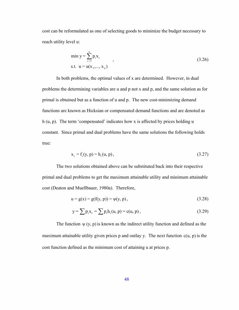
cost can be reformulated as one of selecting goods to minimize the budget necessary to

reach utility level u:

, (3.26)

n

i ii =1

1 n

min y = p x

s.t. u = u(x ,..., x )

∑

In both problems, the optimal values of x are determined. However, in dual

problems the determining variables are u and p not x and p, and the same solution as for

primal is obtained but as a function of u and p. The new cost-minimizing demand

functions are known as Hicksian or compensated demand functions and are denoted as

h (u, p). The term ‘compensated’ indicates how x is affected by prices holding u

constant. Since primal and dual problems have the same solutions the following holds

true:

, (3.27) i i ix = f (y, p) = h (u, p)

The two solutions obtained above can be substituted back into their respective

primal and dual problems to get the maximum attainable utility and minimum attainable

cost (Deaton and Muellbauer, 1980a). Therefore,

, (3.28) u = g(x) = g(f(y, p)) = ψ(y, p)

, (3.29) i i i i y = p x = p h (u, p) = c(u, p)∑ ∑

The function is known as the indirect utility function and defined as the

maximum attainable utility given prices p and outlay y. The next function is the

cost function defined as the minimum cost of attaining u at prices p.

ψ (y, p)

c(u, p)

48

3.2.1 Demand of Textile Products

This and the following sections of the study are adapted from Li (2003). The

theory of maximizing consumers’ utility subject to the budget constraint as discussed

earlier is applied to analyze the fiber equivalent demand. Under the separability

assumption, the fiber equivalent as a group is distinct from all other goods, thus two

groups of consumption goods are available: fiber equivalent and other products

equivalent. The consumption function of an individual can be expressed as:

, (3.30) F NF

F F NF NF

max U = f (X , X )

subject to P ×X + P ×X = I

where

U = total utility

FX = the fiber equivalent available to the individual

NFX = other products equivalents available to the same individual

FP = price of fiber equivalent

NFP = price of other products equivalents.

The budget constraint is the sum of expenditure on textile and non textile products

and is equal to real personal disposable income (I).

The utility function with the budget constraint, expressed in equation (3.23) may

be re-written as:

49

2

F NF i ii =1

φ = U (X , X ) + λ (I - p q )∑ , (3. 31)

solving for the per capita fiber equivalent demand ( ): Fq

, (3.32) F Fq = f (P , P , I)NF

OP , (3.33) F FQ = q * P

where

QF = total fiber equivalent demand

POP = population

Since it is assumed that textile products in India operate in a perfectly competitive

market, an individual’s consumption is hypothesized to be not influenced by another.

Therefore, it is assumed that the total domestic demand for fiber equivalents is the sum of

each individual’s demand given a specific price level.

3.2.2. Cotton Demand

An important assumption in estimating cotton demand is that the fiber mill

demand is greater than or at least equal to the amount of textile products (total fiber

equivalent demand) derived from the first step. The mill’s broad group allocation

problem can thus be expressed as:

50

n

F F i ii =1

F 1 n

Max π = P Q - p q

s.t. Q = f(q ,.., q ) i = 1,..., n

∑ , (3.34)

where

ip = price of ith fiber

= quantity demanded of the iiq th fiber

QF = total fiber equivalent demand

PF = price of fiber equivalent

The solution for (3.34) yields group input demands that have the general form:

* *i i F i jq = q (P , p , p ) i = 1...n, j=1,...,n i j≠ . (3.35)

The share of cotton, wool and man-made fibers among total textile consumption is

estimated using LA/AIDS model.

The Indian fiber market is mainly made up of cotton, wool and man-made fibers,

and textile products are distinct from all other goods indicating that the textile cost

function is weakly separable into two sub-cost functions:

, (3.36) F F NF NFc (W, X) = c (X, c (W , X), c (W , X))

where c (.) is cost function, W denotes the vector of input prices, X the vector of inputs, F

refers to fibers, and NF denotes non-fibers. Applying Shephard’s lemma to the sub-cost

function provides the demand function for a particular fiber. For example, cotton, which

51

itself is a function of total textile production and fiber prices can be expressed by this

equation:

F F

Fcot

cot

δc (W , X) = q (W , X)δW

, (3.37)

LA/AIDS (Linear Approximation/ Almost Ideal Demand System) specified by

Deaton and Muellbauer (1980b) is used to represent the sub-cost function for fibers, and

differentiation of which yield a set of cost-minimizing factors demands. This model

presents a first-order approximation to an arbitrary demand system and uses Price

Independent Generalized Logarithmic (PIGLOG) preferences. Since these preferences

allow exact aggregation across consumers, they represent market demands reflecting the

decisions made by a rational representative consumer. PIGLOG preferences are

represented through the cost or expenditure function, which states the minimum

expenditure necessary to attain a specific utility level at given prices (Deaton and

Muellbauer, 1980b). This cost function is denoted by c (u, p), and PIGLOG is defined by

log c(u, p) = (1 - u) log {a(p)} + u log {b(p)}. , (3.38)

u lies between 0 (subsistence) and 1 (bliss) so that the positive linearly homogeneous

functions of a (p) and b (p) can be regarded as the cost of subsistence and bliss,

respectively. The functional forms for log a (p) and log b (p) are given as,

*0 k k kj k

k k j

1log a (p) = a + α logp + γ logp logp2∑ ∑∑ j , (3.39)

kβ0 kk

log b(p) = log a (p) + β Π p , (3.40)

and, thus AIDS cost function is written as

52

kβ*0 k k kj k j 0 kk k j

1log c (u, p) = α α logp + γ logp logp + uβ Π p2

+∑ ∑∑ k , (3.41)

where , and iα iβ*kjγ are parameters. It can be shown that c (u, p) is linearly

homogeneous in p, which shows it to be a valid representation of preferences. The

demand functions can be derived directly from equation (3.41). The price derivative of

any cost function gives quantity demanded i.e. ii

δc(u,p) = qδp

. Multiplying both sides by

ipc(u,p)

, we get

i ii

i

p qlogc(u,p) = = wlogp c(u,p)

δδ

, (3.42)

wi is the budget share of good i. Logarithmic differentiation of (3.41) provides the

budget shares as a function of prices and utility:

kβi i ij j i 0 kj

w = α + γ logp + β uβ Π p∑ k , (3.43)

where * *ij ij ji

1γ = (γ + γ )2

, (3.44)

Combining these gives Hicksian demand (demand in terms of utility rather than the

income),

kβi i ij j i 0 kji

c(u,p) q = α + γ logp + β uβ Πpp

⎛ ⎞⎜⎝ ⎠

∑ k ⎟ , (3.45)

Inverting the cost function and expressing u as a function of p and y, and the fact that

income is equal to expenditure gives

53

kβ*0 k k ij k j 0 i kk k j

1log y = α + α logp + γ logp logp + uβ β Π p2∑ ∑∑ k , (3.46)

k k

*0 k k ij k

k k jβ β

0 k 0 kk k

1α + α logp + γ logp logp2logyu = -

β Π p β Π p

∑ ∑∑ j

, (3.47)

Substitution of u into the share equations allows the expenditure shares to appear as a

function of income and all prices. This is also the equation that is usually estimated.

k

k k

*0 k k ij k j

k k jβi i ij j 0 i k β βkj 0 k 0 kk k

1α + α logp + γ logp logp2logyw = α + γ logp + β β Π p -

β Π p β Π p

⎛ ⎞⎜ ⎟⎜ ⎟⎜ ⎟⎜ ⎟⎝ ⎠

∑ ∑∑∑ ,

(3.48)

AIDS demand function in the budget share form can thus be written as

i i ij j ij

w = α + γ logp + β log{y/p}∑ , (3.49)

where p is a price index defined by

*0 k k kj k

k j k

1log p = α + α logp + γ logp logp2∑ ∑∑ j

k

, (3.50)

If p is approximated by the Stone geometric price index p*,

, (3.51) kk

log p* = w logp∑

The model that uses Stone’s price index is known as the “Linear Approximate AIDS”

(LA/AIDS) (Green and Alston, 1990). From equation (3.49) we get the share of cotton,

54

man-made and wool fiber. To represent a system of demand equation, equation (3.49)

must hold the following restrictions:

Adding up: , (3.52) n n n

i ij ii =1 i =1 i =1α = 1 γ = 0 β = 0∑ ∑ ∑

Homogeneity: , (3.53) ijjγ = 0∑

Symmetry: , (3.54) ij jiγ = γ

Adding-up and homogeneity restrictions show that the demand equation follows a

linear budget constraint. Symmetry is a guarantee of and a test of the consumer’s

consistency of choice. Inconsistent choices are made in the absence of symmetry.

Following Green and Alston (1990), the Marshallian (uncompensated) and the

Hicksian (compensated) elasticities, as well as the expenditure elasticities in the

LA/AIDS model can be computed from the estimated coefficients as follows.

Uncompensated elasticities:

The Almost Ideal Demand System (AIDS) is derived in budget share form as:

( )i ii ij j i

j

p q = α + γ logp + β log y/Py ∑ ,

Own-price elasticities:

Rearranging the above equation, keeping only qi on the left side and then taking partial

derivative with respect to pi:

( ) jii ij j i ii i2 2

ji i i

ywq y y = - α + γ logp + β log y/P + γ - βp p p p

⎛ ⎞∂⎜ ⎟∂ ⎝ ⎠

∑ 2i

, and

55

iiii i

i

γη = -1 + - β ,w

(3.55)

Cross-price elasticities:

jiii i

i j i j

wq y 1 y = γ - βpj p p p p

⎛ ⎞∂⎜ ⎟⎜ ⎟∂ ⎝ ⎠

ij i jij

i i

γ β wη = - ,

w w (3.56)

Expenditure elasticities:

( )i ii ij j i

ji i

q β p q β1 1 = α + γ logp + β log y/P + = + p py⎛ ⎞ ⎛ ⎞∂⎜ ⎟ ⎜ ⎟∂ ⎝ ⎠⎝ ⎠

∑ i i i

i ip y p,

ii

i

βη = 1 + w

, (3.57)

Hicksian elasticities:

Own-price elasticities:

, (3.58) *ii ii i iη = η +w η

Cross-price elasticities:

, (3.59) *ij ij j iη = η + w η

A good can be categorized according to the signs and magnitudes of the

elasticities. If the absolute value of the own price elasticity is less than 1, the demand of

that commodity is inelastic, while if it is greater than 1, the demand is elastic. On the

other hand, the own price elasticity is positive for the Giffen good. Positive cross price

elasticity suggests that the commodities are substitutes, while the commodities are

complements if it is negative. Similarly, the commodity is said to be normal when the

56

expenditure elasticity is positive, while the commodity is inferior if it is negative. The

normal good is said to be a luxury when expenditure elasticity is more than one and a

necessity when it is between zero and one.

3.3. Competitiveness of U.S. Cotton

It could be conceptualized that the demand for U.S. cotton in the Indian market is

price inelastic because of quality differential between cotton imported from the United

States and Australia/rest of the world. India primarily imports the extra long staple (ELS)

cotton from the United States, which is a premium cotton and is preferred for apparel.

On the other hand, the demand for cotton from Australia/rest of the world are likely to be

price elastic because cotton imported from Australia and the rest of the world are

medium/short staple, which is preferred for denim manufacturing and can be substituted

with domestic cotton. Thus, it is hypothesized that import demand for the U.S. cotton

will be expenditure elastic, implying that U.S. market share in the Indian market will go

up as the import demand for cotton in India increases.

The model used for this study is based on the assumption that decisions on

imports by the Indian textile industry are made based upon a two-stage budgeting

process. In the first stage, the importer (India) decides how much cotton to import. In

the second stage, given the total amount imported, the importer decides how much to

import from each supplier (U.S., Australia, and the rest of the world).

57

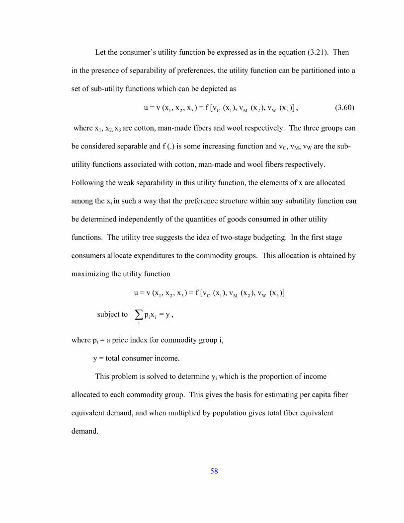
Let the consumer’s utility function be expressed as in the equation (3.21). Then

in the presence of separability of preferences, the utility function can be partitioned into a

set of sub-utility functions which can be depicted as

1 2 3 C 1 M 2 W 3u = v (x , x , x ) = f [v (x ), v (x ), v (x )] , (3.60)

where x1, x2, x3 are cotton, man-made fibers and wool respectively. The three groups can

be considered separable and f (.) is some increasing function and vC, vM, vW are the sub-

utility functions associated with cotton, man-made and wool fibers respectively.

Following the weak separability in this utility function, the elements of x are allocated

among the xi in such a way that the preference structure within any subutility function can

be determined independently of the quantities of goods consumed in other utility

functions. The utility tree suggests the idea of two-stage budgeting. In the first stage

consumers allocate expenditures to the commodity groups. This allocation is obtained by

maximizing the utility function

subject to ,

1 2 3 C 1 M 2 W 3u = v (x , x , x ) = f [v (x ), v (x ), v (x )]

i ii

p x = y∑

where pi = a price index for commodity group i,

y = total consumer income.

This problem is solved to determine yi which is the proportion of income

allocated to each commodity group. This gives the basis for estimating per capita fiber

equivalent demand, and when multiplied by population gives total fiber equivalent

demand.

58

3.3.1. Cotton Import Demand

In the second stage, consumers’ group expenditures are allocated to the individual

commodities (in this study the U.S., Australia and ROW). This is done by maximizing

sub-utility function for each group subject to the amount of expenditure determined in the

first stage of budget allocation (Colmen and Thigpen, 1991). This is given by,

Max i iv (x )

Subject to i i ii

p x = y∑ ,

where pi is a vector of individual commodity prices associated with xi. The solution to

this problem gives the demand function for each element of xi, in this case, the demand

for U.S., Australia and the ROW which can be shown as:

i i i ix = x (p , y ) , (3.61)

3.4. Summary

This chapter graphically presents the effects of the MFA quota elimination on

Indian and world cotton markets. The analysis provides the directional change of the

effects and suggests that the expected effects of textile quota elimination would be to

increase Indian textile exports, increase Indian cotton imports, increase world price,

increase rest of the world production, and exports. Cotton supply response

conceptualizes two dynamic processes. First, farmers make planting decision based on

their expectation of prices to be received after harvesting, which occurs several months

after planting. Thus, a time lag occurs in agricultural production, which makes the

59

modeling of expectations formation a key issue in the area of agricultural supply response

analysis. Second, the observed acreage and desired acreage differ because of adjustment

lags in the reallocation of variable factors. It may take several years for farmers to reach

their desired acreage level once the price changes. Therefore, specifying adjustment lags

clearly becomes necessary in the model. This dynamic behavior has been captured by the

Nerlovian model where desired acreage is conceptualized to depend upon expected

prices.

Man-made fiber capacity is determined at the point where short-run and long-run

cost functions are tangent to each other. Optimal output for man-made fiber, on the other

hand, is determined by solving the Lagrangian for the profit-maximization constrained by

input limits. Man-made fiber capacity utilization is obtained as the ratio of optimal

output and man-made fiber capacity.

Cotton demand is derived using a two-step process - first the fiber equivalent

quantity of the textile is conceptualized, followed by the cotton demand in the second

stage. Similarly, competitiveness of U.S. cotton is conceptualized on the assumption of

two-stage budgeting procedures, where the importer (India) decides how much cotton to

import in the first stage, while in the second, given the total amount imported, the

importer decides how much to import from each supplier.

60

CHAPTER IV

METHODS AND PROCEDURES

For the purpose of this study, a partial equilibrium structural econometric model

of Indian fiber markets was developed to measure the effects of MFA quota elimination

on Indian cotton trade. Schematic representation of the Indian fiber model, which depicts

the relationships among different components of the model, is presented in figure 4.1.

The framework includes supply, demand, and price linkages equations for cotton and

man-made fibers.

The discussion of the conceptual framework in the beginning of the last chapter

revealed that the expected effects of MFA quota elimination would be to increase Textile

exports, cotton imports, world price, and cotton production. However, the analysis only

revealed the directional change; the change in magnitudes will be determined by the

demand and supply elasticities for which econometric model of the Indian fiber is

developed, which is depicted in Figure 4.1. As shown in the diagram, acreage and yield

levels contribute to cotton production, which builds up total domestic supply after

incorporating beginning stocks and imports. Indian cotton supply responses are

estimated in a regional framework. Cotton-producing area in India is segregated into four

regions in order to account for heterogeneity in growing conditions arising out of climatic

differences, availability of water, and other natural resources that influence the mix of

crops in each of the regions. This is important because liberalization of domestic

agricultural policies is likely to have varying effects on the different cotton-producing

61

Cotton Area

CottonYield

Cotton Production

BeginningStocks

Cotton ImportsA-Index

Domestic Cotton Supply

Cotton Consumption

MarketEquilibrium

CottonExports

Cotton EndingStocks

Apparel Demand

IndustrialDemand

Total Fiber Consumption

Cotton Mill Use Wool Mill

UseMan-madeFiber Mill

Use

Polyester Price

Textile Trade

MarketEquilibrium

Man-madeFiber

Utilization

Man-made Fiber

Capacity

Man-madeFiber

Production

A-Index

Domestic CottonPrice

Man Made Fiber Net Trade

Exogenous Variable

Endogenous Variable

62

Figure 4.1. Schematic Representation of the Indian Fiber Model

regions. Thus, the disaggregated supply model, i.e., four regional models, will avoid the

aggregation bias. The four regions are comprised of northern, central, southern, and rest

of India.

The structural Indian fiber model also takes into account inter-fiber competition

among cotton, wool, and man-made fibers at the mill level. This allows for substitution

between cotton and man-made fibers based on their relative prices. Mill utilization of

each fiber is estimated in two steps (Figure 4.1): (1) total textile consumption, and (2)

allocation of textile consumption among various fibers such as cotton, man-made fibers,

and other fibers based on the relative prices. Thus, the second step yields domestic mill

use demands of cotton, wool, and man-made fiber in the Indian fiber model. Cotton

ending stocks and cotton trade must also be taken into account in the cotton component in

order to close the model. Total cotton supply and total cotton demand in equilibrium

determine the domestic cotton price. Total cotton demand includes domestic cotton mill

utilization, ending stocks, and exports.

Similarly, man-made fiber production (Figure 4.1) is estimated as the product of

capacity and utilization rate. Man-made fiber production and man-made fiber demand,

domestic mill use and net trade combined, determine market clearing conditions for the

man-made fiber sector. This enables to solve the man-made fiber price endogenously in

the model to allow inter-fiber substitution at the mill level. Finally, world cotton price

(A-Index Price) enters into the model through cotton trade equations.

63

After choosing the appropriate framework according to the stated objectives, the

next step is the specification and estimation of cotton, man-made fiber and textile supply,

demand, and trade equations. The specified equations are estimated using ordinary least

squares (OLS), two-stage least squares (2SLS), and seemingly unrelated regression

(SUR), as appropriate. Policy simulation is discussed next, followed by competitiveness

of U.S. cotton. The next section discuss the validation, where the models are evaluated

using signs and magnitude of the parameters, and are also tested for their statistical

validity using t-test, F-test, R-squared value, Theil’s inequality coefficients, and

decompositions of mean squared errors. Finally, data sources are discussed; and the

chapter ends with a summary.

4.1. Model Specification

In this section, each behavioral equation is specified based on the conceptual

framework developed in the previous chapter. In addition, proper functional forms and

appropriate lag structure of the variables, which provide a good fit as well as reasonable

elasticity measures, are chosen.

4.1.1. Fiber Supply Estimation:

4.1.1.1. Cotton Supply Model:

In this study, the Indian cotton-producing area is segregated into four regions in

order to account for heterogeneity in growing conditions arising out of climatic

differences, availability of water, and other natural resources that influence the mix of

64

crops in each of the regions. The four regions include north, central, south and the rest of

India. The ith region acreage response is specified as:

, (4.1) i t i, t i, t i, t-1AC = f(EPC , EPCM , AC )

where i=north, central, south, and the others regions in India. is the cotton acreage

in i

i tAC

th region in time t; represents expected cotton price in ii, tEPC th region in time t;

are the expected prices of competing crops in the ii, tEPCM th region in time t.

Competing crops for the northern region include wheat, rice and rapeseed; for the

central region, include sugarcane, groundnut, rapeseed, and wheat, while groundnut,

corn, sugarcane, and rice are the competing crops for the southern region. The area

devoted to cotton is expected to be positively related to the price of cotton and negatively

related to the prices of competing crops. Expected prices are calculated as the weighted

average of the current year’s minimum support price and last year’s average market

prices for the corresponding crops. Weight for the support price is based on the

proportion of cotton procured by the government (e.g., 18.8 and 19.5 percent in 2002, and

in 2003).

Cotton yield is specified as follows.

, (4.2) i t i, t i, t-1 t t tYC = f (EPC , YC , RF , FA , T )

where represents cotton yield in the ii tYC th region; is cotton yield lagged one year

in the i

i, t-1YC

th region; represents rainfall in millimeter; and is the fertilizer application

in Kilogram/Hectare. Cotton is very sensitive to rainfall. Heavy or scanty rainfall at

tRF tFA

65

critical times of the growth period may cause decline in yield. Additionally, an optimum

application of fertilizer may increase the yield.

Once cotton area and yield have been estimated, cotton production can be

calculated by multiplying area by yield and sum over all four regions:

, (4.3) 4

t i t i=1

CPR = AC *YC∑ i t

where represents total cotton production in India in time period t. tCPR

4.1.1.2. Man-made Fiber Supply Model:

In this model, man-made fiber mill use, the components of man-made fiber

production, man-made fiber capacity, and utilization, are all determined endogenously.

The specifications of man-made fiber production capacity, utilization, and net trade

equations are similar to Li (2003). Following the conceptual framework (3.1.2) derived

in the previous chapter, man-made fiber production capacity is specified as a function of

polyester and crude oil prices lagged three to six years, and man-made fiber production

capacity lagged one year.

, (4.4) t t - k t - k t-1MMPC = f (PP , PO , MMPC )

where represents the man-made fiber productive capacity at time t; is the

lagged price of polyester; is the lagged price of petroleum crude oil;

represents the man-made fiber productive capacity at time t-1, and k = 3, …, 6.

tMMPC t - kPP

t - kPO t-1MMPC

Man-made fiber capacity utilization is specified as the function of polyester and

crude oil prices, and utilization rate lagged one year:

66

, (4.5) t t t t-1MMCUZ = f (PP , PO , MMCUZ , T)

where MMCUZt is the man-made fiber capacity utilization in period t.

4.1.2. Fiber Demand Estimation:

As discussed in the conceptual framework, fiber demand is derived using a two-

step process. In the first step, consumers allocate expenditures to a broad group of

commodities, i.e., per capita textile consumption in fiber equivalent in India is estimated

and then allocated among various fibers in the second stage.

Textile consumption (per capita textile demand in fiber equivalent) is specified as

the function of textile price index, food price index, per capita real income, and time

trend:

t t t tTXPC = f (PTX , PFD , I , T) , (4.6)

where TXPCt is the per capita textile demand in fiber equivalent in time t; is the

textile price index; is the food price index; represents per capita income, and T

represents time trend. Because of economic expansion, consumers will have higher

disposable income resulting in elevated purchasing power, and higher demand for various

products, including textiles and clothing. Thus, textile consumption is hypothesized to be

positively related to income. In addition, economic theory suggests that consumption of

a good is inversely related to its own price and positively related to the prices of

competing goods. Thus, textile consumption is expected to have an inverse relationship

with the textile price index and a direct relationship with the food price index. Equation

(4.6) is estimated by using the OLS method.

tPTX

tPFD tI

67

In the second stage, the share of each of the fibers in the textile consumption

framework is estimated using a LA/AIDS model. The empirical LA/AIDS model for the

cotton, man-made fiber, and wool shares for Indian textiles is specified as follows:

t 1 11 t 12 t 13 t 1 1tYSC =α + γ log(PC ) + γ log(PMF ) + γ log(PW ) + β log + uP*

⎛ ⎞⎜ ⎟⎝ ⎠

, (4.7)

t 2 21 t 22 t 23 t 2 2 tYSMF = α + γ log(PC ) + γ log(PMF ) + γ log(PW ) +β log + uP*

⎛ ⎞⎜ ⎟⎝ ⎠

, (4.8)

t 3 31 t 32 t 33 t 3 3 tYSW = α + γ log(PC ) + γ log(PMF ) + γ log(PW ) + β log + uP*

⎛ ⎞⎜ ⎟⎝ ⎠

, (4.9)

where is the price of cotton; is the price of man-made fiber; is the price of

wool; Y is the total fiber expenditure; is the stone price index; is the share of

cotton fiber in the textile; is the share of manmade fiber, and represents the

share of wool.

tPC tPMF tPW

P* tSC

tSMF tSW

Total Mill demand of the individual fiber in India can be estimated by multiplying

respective fiber shares with total textile consumption and population as

, (4.10) t t tDC = TXPC *SC *PO tP

t

tP

t t tDMF = TXPC *SMF *POP , (4.11)

t t tDW = TXPC *SW *PO , (4.12)

where , , are the total mill demand of cotton, man-made fiber, and

wool, respectively, and POP

tDC tDMF tDW

t represents the total population of India in time t.

68

4.1.3. Cotton Ending Stocks and Trade Equations:

Cotton ending stocks can be specified as the function of domestic cotton price,

cotton production, and beginning stock.

, (4.13) t t t-1CES = f(PC , CES , CPR )t

t

where is the cotton ending stocks. Both beginning stocks and cotton production

variables are expected to have a direct relationship with ending stocks; at the same time,

the cotton market price is expected to have an inverse relationship with ending stocks.

Equation (4.13) is estimated using the OLS method.

tCES

Cotton export in India is specified to depend on relative prices between domestic

and world markets, and cotton supply. The exchange rate is not modeled explicitly here

but it is captured in the model by expressing international price in domestic currency after

adjusting for export tax:

, (4.14) t t t t tCEX = f (PC , PA * (1 - ET )*XR , CSU )

where is the export of cotton; PAtCEX t is the international cotton price represented by

A-Index c.i.f. North Europe; is the cotton supply; the export tax on cotton in

percentage, and is the exchange rate of U.S. dollars into Indian currency. Cotton

exports should increase with a rise in international cotton prices relative to domestic price

and vice-versa. In addition, a greater supply of cotton means that more cotton can be

exported owing to high international price, thus a direct relationship is hypothesized

between supply of cotton and export of cotton. The cotton export equation is estimated

using the OLS method.

tCSU tET

tXR

69

The cotton import equation is specified as the function of the relative domestic

price of cotton with respect to the international price adjusted for the import tariff, and

Income.

t t t t tCIM = f (PC , PA *(1+IT )*XR , I )t , (4.15)

where CIMt is the import of cotton at time t; is the import tariff rate in India in

percentage, and gross domestic product represents the proxy for income ( ) in India. It

is assumed that as increases and the international prices of cotton relative to domestic

price decreases, cotton import demand should increases; that is, more cotton fiber will be

imported. The cotton import equation is estimated by the OLS method.

tIT

tI

tI

4.1.4. Market Clearing Condition:

Finally, an identity equation is added to solve the system of demand and supply

equations for equilibrium prices and quantities of cotton. The equilibrium condition

exists at the point where total cotton consumption is equal to total cotton supply in India.

This can be specified as in the following equation:

t t-1 t t tCPR + CES + CIM = DC + CES + CEX . t

tR

(4.16)

Similarly, the man-made fiber market clearing condition includes production,

consumption, and net trade. Since ending stocks data is not available, it is assumed that

stock does not change from year to year.

, (4.17) t tMMPR = DMF + MMT

70

where represents man-made fiber production, which is obtained through

multiplying man-made fiber capacity utilization with its capacity; is the man-made

fiber consumption, and is the man-made fiber net trade (exports - imports).

tMMPR

tDMF

tMMTR

All the above equations except those of LA/AIDS models are estimated using

OLS. A battery of statistical methods is used to test whether the assumptions of normal,

independent, and identically distributed (NIID) error terms are violated and whether these

violations cause a bias in their estimators. The assumption of homoskedastic conditional

variance is tested using the White’s test and Cook-Weisburbg test. For testing whether

the errors are linear with respect to the conditioning variables, the Respecification Error

Test (RESET) developed by Ramsey is used. To test the assumption of a normal

conditional distribution, the skewness-kurtosis (SK) test, the Shapiro-Wilk (SW) test, and

a graph of the conditional distribution with a normal curve overlay are used. If

heteroskedasticity, autocorrelation, and non-normality are detected, these are corrected

before estimation.

The LA/AIDS model for share of fiber is estimated first without any restrictions

and later, imposing adding-up, homogeneity and symmetry restrictions combined. The

error terms across the equations in LA/AIDS models are correlated by the fact that the

dependent variables need to satisfy the budget constraint. Consequently, the OLS

estimates of these equations would be inconsistent and biased. Therefore, Seemingly

Unrelated Regressions (SUR), which provide more efficient estimates are used instead.

In the first stage, OLS is used to estimate the variance-covariance matrix among the

residuals, while in the second stage, the estimated matrix is used in a generalized least

71

squares estimation. Imposing of the adding-up restriction makes the variance-covariance

matrix for the disturbances singular, thus, non-singularity is maintained by deleting the

equation of Rest of the World (ROW) from the fiber share empirical LA/AIDS model.

The parameters associated with the omitted demand equation are recovered later on by

making use of the restrictions. Correction for autocorrelation is done in the estimation of

parameters, and a non-linear algorithm is used for the estimation of the LA/AIDS model.

All the equations are estimated using SAS (SAS Version 9.1, 2002-2003).

4.2. Policy Simulations

In this study, the results of the estimated econometric model were used to

develop baseline projections for supply, demand, and prices of cotton, man-made fibers,

and textiles, assuming the continuation of the current policies including MFA quotas in

textile and apparel exports. Projections for macroeconomic variables such as real GDP,

consumer price index (CPI), exchange rates, and population were obtained from the 2004

World and U.S. Agricultural Outlook published by Food and Agricultural Policy

Research Institute (FAPRI). The baseline projections for India and the world cotton

market were developed for a span of ten years ranging from 2004/05 to 2014/15 by

linking the Indian fiber model to the existing world fibers model at Texas Tech

University. Linking the Indian model with the world model allowed the world cotton and

man-made fiber prices to be determined endogenously.

Once the baseline projections were developed, scenario projections were

generated by removing MFA quotas. Three scenarios were performed, and these were

72

10, 20, and 30 percent increase in textile exports from India. In the baseline projection,

all the exogenous variables were assumed to be constant, whereas scenario projections

were run by changing exogenous variables of interest (textile exports) in the model. In

both projections, simulation was done until the values of endogenous variables do not

change any more. The policy effects are measured by comparing the differences between

the scenario and the baseline projections.

4.3. Competitiveness of U.S. cotton

After measuring the effects of MFA quota eliminations on the Indian cotton market,

particularly on its cotton imports, the next step was to determine whether U.S. cotton is

competitive enough to capture additional market shares. Competitiveness of U.S. cotton

in Indian market was determined by estimating Indian cotton import demand by origin

using a LA/AIDS model. The LA/AIDS model was estimated first without any

restrictions and later imposing adding-up, homogeneity, and symmetry restrictions

combined. The empirical LA/AIDS model for the USA, Australian and the rest of the

world cotton import demand was specified as follows and are estimated using SHAZAM

(SHAZAM, 2002):

vUSA 1 11 USA 12 AUS 13 ROW 1 1t

v

YW = µ + δ log(P ) + δ log(P ) + δ log(P ) + λ log + uP *

⎛ ⎞⎜ ⎟⎝ ⎠

(4.18)

vAUS 2 21 USA 22 AUS 23 ROW 2 2t

v

YW = µ + δ log(P ) + δ log(P ) + δ log(P ) + λ log + uP *

⎛ ⎞⎜ ⎟⎝ ⎠

(4.19)

vROW 3 31 USA 32 AUS 33 ROW 3 3t

v

YW = µ + δ log(P ) + δ log(P ) + δ log(P ) + λ log + uP *

⎛ ⎞⎜ ⎟⎝ ⎠

(4.20)

73

where are, respectively, the value of market share of the United

States, Australia, and the rest of the world, while are the unit import

values of cotton from the United States, Australia, and the Rest of the World,

respectively. is the Stone price index, is the value of total cotton imports in

India, and are the error terms, associated with the share equations for the

USA, Australia, and the rest of the world, respectively. The error terms,

are assumed to be normally distributed with constant means and

variances, and may be contemporaneously correlated.

USAW , AUSW , ROWW

USAP , AUSP , ROWP

vP * vY

1tu , 2 tu , 3tu

21t 2t 3tu , u , u ~N(µ, σ )

The estimated import demand elasticities of Indian cotton will be used to

determine whether U.S. cotton is competitive enough to capture additional market shares

when situations arise. Own-price, cross-price, and expenditure elasticities for the U.S.

will be compared with that of Australia and the rest of the world. Positive cross-price

elasticities indicate that cotton is substitute for those countries, while negative value

implies it is complement. Large expenditure elasticity suggests the cotton of that country

is of premium quality and is preferred for apparel.

4.4. Model Validation

Model validation is undertaken by using the standard t-tests, F-tests, and R2

procedures where applicable in this analysis. Mean Squared Error (MSE) and Theil’s

inequality coefficient techniques are applied to assess the overall reliability of each

74

model. Theil’s inequality coefficient test is formulated and discussed as follows

(Pindyck and Rubinfeld, 1998):

( )

( ) ( )

T 2s at t

i=1

T T2 2s at t

i=1 i=1

1 Y -YTU =

1 1Y + YT T

∑

∑ ∑, (4.21)

The numerator of the U-statistic is the Root-Mean-Squared Error (RMSE). However, the

denominator is scaled in such a way that U is always between 0 and 1. U = 0 indicates a

perfect fit because = for all t, while U = 1 suggests the model is a poor fit. Thus

the Theil’s inequality coefficient measures the RMSE in relative terms.

stY a

tY

The MSE measures the mean of the squared deviation between simulated and

actual variables, and is expressed as:

T

s at t

t=1

1MSE = (Y -Y )T∑

2 , (4.22)

Where Yst = simulated value of the endogenous variable at time t,

Yat = actual value of the endogenous variable at time t, and

T = number of periods in the simulation.

MSE depends upon the units in which the variable is expressed. The magnitude of the

error does not give any indication of how large the error is, therefore, this error can be

assessed only by comparing it with the average size of the variable in question.

However, the main advantage of MSE is that it can be decomposed into various

components, which show the deviation between the simulated and actual values. Two

methods of decomposition exist: first, by Theil, and second, by Maddala.

75

Pindyck and Rubinfeld (1998) mention the Theil’s decomposition of MSE as

follows:

( ) ( ) ( ) ( )2 2 2s a s a

t t s a s a1 Y -Y = Y -Y + σ -σ + 2 1-ρ σ σT∑ , (4.23)

where sY , are the mean and standard deviation of the series ; and sσstY aY , are the

mean and standard deviation of the series ; and ρ is the correlation coefficient for the

two series. Rearranging, equation 4.23 can be written as,

aσ

atY

( )( )

( )

( )( )

( )

2 2s as a s a

2 2s a s a s at t t t t t

Y -Y σ -σ 2 1-ρ σ σ1 + + 1 1 1Y -Y Y -Y Y -Y

T T T

=∑ ∑ ∑

2 (4.24)

where

( )( )

2s a

2s at t

Y -YUM = 1 Y -Y

T∑, (4.25)

( )

( )

2s a

2s at t

σ -σUS = 1 Y -Y

T∑ , (4.26)

( )

( )s a

2s at t

2 1-ρ σ σUC = 1 Y -Y

T∑ , (4.27)

where , , are the bias, variance and covariance proportions of U,

respectively; and the sum of these three is equal to one.

UM US UC

The represents the systematic error and it is expected to be equal to zero. A

larger value of (above 0.1 or 0.2) suggests the presence of systematic bias. A large

value of US , which is the variance proportion, implies that the actual series has more

UM

UM

76

fluctuation than the simulated series or vice versa, and thus it becomes necessary to

revise the model. Finally, the covariance proportion, , measures the unsystematic

error and is less worrisome than the other two.

UC

According to Coleman and Thigpen (1991), the second decomposition of MSE by

Maddala, consists of bias (UM), regression (UR), and disturbance (UD) terms, and they

are derived as follows:

( ) ( ) ( ) ( )2 2 2s a s a 2t t s a

1 Y -Y = Y -Y + σ -ρσ + 1-ρ σT∑

2a (4.28)

Equation 4.28, after rearrangement, can be written as:

( )( )

( )

( )( )( )

2 2s a 2 2as a

2 2s a s a s at t t t t t

Y -Y 1-ρ σσ -ρσ 1= + + 1 1 1Y -Y Y -Y Y -Y

T T T∑ ∑ ∑2

(4.29)

where

( )( )

2s a

2s at t

Y -Y UM = 1 Y -Y

T∑ (4.30)

( )

( )

2s a

2s at t

σ -ρσ UR = 1 Y -Y

T∑ (4.31)

( )( )

2 2a

2s at t

1-ρ σ UD = 1 Y -Y

T∑ (4.32)

where UM, UR, UD are the bias, regression, and disturbance components of U. The

sum of UM, UR, and UD equals one. The UM and UR components capture the

systematic divergence of the prediction from actual values. Therefore, for a model that

77

fits the data well, the proportion of UM and UR should approach zero. The UD

component, which captures the random divergence of the prediction from the actual

values should approach one.

4.5. Data Requirements

Data were collected from various sources. Macroeconomic variables for India

such as GDP, population, exchange rate, GDP deflator and the average spot price of

crude oil were obtained from “International Financial Statistics” published by the

International Monetary Fund (IMF). Cotton A-Index price, US 1.5 denier polyester price,

and US farm price sheer wool (greasy basis) were collected from Cotton and Wool

Yearbook of Economic Research Service, United States Department of Agriculture (ERS,

USDA). Prices of polyester staple fiber and cotton fiber, and cotton tariff/duty in India

were obtained from Foreign Agricultural Service, USDA and the Textile Commissioner’s

Office, Government of India (GOI). Minimum Support Price for cotton and competing

crops were obtained from the web site of India’s Ministry of Agriculture (available on-

line at http:// agricoop.nic.in/statistics/). The Textile Price Index was gathered from the

Handbook of Industrial Policy and Statistics 2001, India; at the same time, Wholesale

Price Index for food was obtained from the Handbook of Statistics on Indian Economy,

2001 on CD-ROM. Both indices were originally available on 1970/71 and 1981/82 base

years, which were converted to1993/94 base year for consistency. The Textile Price

Index for the year 1982-84 was missing and had to be interpolated. The producer price

for cotton and competing crops was obtained from the data base of Food and Agricultural

78

Organization (FAO). The Consumer Price Index was gathered from the Ministry of

Finance, GOI. Total fiber consumption, total cotton consumption, and total manmade

fiber consumption were obtained from the Foreign Agricultural Services of the United

States Department of Agriculture (FAS/USDA), and the Textile Commissioner’s Office,

GOI. Wool and other fiber consumption were calculated by subtracting cotton and man-

made from total fiber consumption. Similarly, man-made fiber capacity, utilization and

man-made fiber production were also collected from the same sources.

Data for cotton supply and demand was obtained from the FAS/USDA. The

database consists of cotton area, yield, production, imports, exports, ending stocks, and

total domestic consumption. The area, yield, and production data for cotton at the state

level were obtained from the FAS/USDA, Indiastat.com and the Ministry of Agriculture,

India on-line. The yield data for competing crops at the state level were gathered from

the Centre for Monitoring Indian Economy, and the Directory of Indian Agriculture,

1997. Fertilizer consumption was obtained from the Centre for Monitoring Indian

Economy. The percentage of coverage under irrigation was collected from the

Department of Agriculture and Cooperatives, India (available on-line at

http://agricoop.nic.in/statistics/), while rainfall data was collected from Indiastat.com.

Although the data were obtained from various sources, these were cross-checked for

consistency.

Data used in the study of the competitiveness of United States cotton in India

are the annual data for import value and net weight for the period of 1988 to 2002. Data

for the United States, Australia, and the other countries, which are consistent and major

79

suppliers of raw cotton to India, were collected from the website of “Commodity Trade

Statistics” published by the United Nations. The unit import values (equivalent to c.i.f.

prices) were calculated by dividing the total import value by total import volume (net

weight) for each country. Average cotton market shares (in value terms) during the study

period of 1988-2002 are 13.61 percent, 11.56 percent, and 74.83 percent for the United

States, Australia, and the rest of the world, respectively.

4.6. Summary

Supply, demand, and trade equations are specified for cotton and manmade fibers

based on the conceptual analysis developed in the previous chapter. An identity equating

cotton supply with cotton demand cleared the cotton market and determined the cotton

price endogenously. The man-made fiber markets were closed with an identity, which

determines man-made fiber net trade. An expected price was used in the area equation of

cotton in line with the Nerlovian model. This expected price was expressed as the

weighted average of the current year’s minimum support price and the last year’s market

prices for the corresponding crops. Similarly, to estimate individual fiber share in the

textile, textile consumption was estimated in the first stage, whereas individual fiber

share was estimated from textile consumption in the second stage using the LA/AIDS

model. Per capita fiber demand was calculated as the product of textile consumption

with individual fiber share.

A battery of statistical methods were used to test whether the assumptions of

normal, independent, and identically distributed (N.I.I.D.) of error term are violated and

80

whether these violations cause a bias in their estimators. All the equations except those

of the LA/AIDS models were estimated using OLS.

The estimated model was used to develop ten-year (2004-2014) baseline

projection for supply, demand, prices, and trade flows of cotton and man-made fibers. In

the next step, a MFA elimination scenario was developed and compared with the baseline

projections to measure the policy effects. Projections for exogenous parameters were

taken from the study of FAPRI, 2004.

The competitiveness of U.S. cotton in the Indian market was specified and

estimated to determine whether U.S. cotton was competitive enough to capture additional

market shares. Validation of the models was done to assess the overall reliability of each

model using MSE and Theil’s inequality coefficient. Various prices and income data

were deflated using appropriate deflators and were adjusted for exchange rates before

estimation. As data were collected from various sources, they were tested for

consistency.

81

CHAPTER V

RESULTS AND DISCUSSIONS

The results of the various components of the partial equilibrium model along with

simulation results are presented and discussed in this chapter. It opens with the reporting

and discussion of the estimated parameters of supply, demand, and trade equations as

well as model validation statistics. The chapter then proceeds with the discussion of

macroeconomic assumptions required for developing ten-year baseline projections for the

period of 2004/05 to 2014/15. The baseline model is then used to conduct policy

simulation by removing textile quotas. This section provides the comparison of the

baseline and scenario results and highlights the effects of MFA quota eliminations.

Finally, competitiveness of the U.S. cotton in the Indian market is reported, and policy

implications are discussed.

5.1. Fiber Supply Model

5.1.1. Cotton Acreage Model:

The regional cotton acreage models were estimated using OLS for the period

1970-2003. The adjusted R2 for the cotton acreage models for northern, central, and

southern regions are 0.73, 0.62 and 0.49, respectively. This implies that 73, 62 and 49

percent of variations in the acreage in the respective regions are explained by the

explanatory variables included in the equations. The estimated parameters along with the

diagnostic statistics are presented in Table 5.1. The cotton acreage was specified as the

82

Table 5.1: Regression Results of Indian Regional Cotton Acreage Models Northern Central Southern

Intercept 587.06* (289.98)

4115.38*** (593.03)

1431.15*** (185.73)

EPC 0.88* (0.46)

2.04** (0.92)

1.71*** (0.53)

EPCM1 -6.97* (3.91)

-7.94** (3.77)

EPCM2 -19.71*** (5.83)

T 27.34* (15.38)

LAC1 0.64*** (0.14)

LYC2 4102.86** (1911.69)

D02 -309.94** (133.11)

D86

-604.96*** (166.81)

DW Statistic

1.70 2.15

DH Statistic

1.92

Adj. R2 0.73

0.62 0.49

F-Stat 17.44***

10.22*** 8.97***

Notes: Standard errors are reported in the parentheses below the coefficients. * indicates significance at the 10 percent level, ** indicates significance at the 5 percent level, and *** indicates significance at the 1 percent level.

83

function of the expected prices of cotton, expected prices of competing crops, and lagged

acreage.

For the northern region, in addition to expected price of cotton (EPC), expected

price of rice (EPCM1) as the competing crop, and lagged cotton acreage (LAC1), a

dummy variable (D02) was included to represent drought in 2002. The estimated

coefficients of own and competing crop price (rice) have the expected signs and are

statistically significant at the 10 percent significance level, implying that cotton acreage

tends to increase with an increase in the expected price of cotton and cotton acreage tends

to decrease with an increase in the price of rice. The statistically significant coefficient

on the lagged cotton acreage (LAC1) demonstrates fixity in cotton production. Farming

in the northern region is highly mechanized relative to the other parts of India. Since

cotton is a capital intensive crop, it makes it difficult for the producers to switch to other

crops in the short-run based on relative returns. The dummy variable D02 captured the

decline in cotton acreage due to severe drought in 2002.

Similarly, cotton acreage for central region was specified as the function of

expected price of cotton, price of groundnut (EPCM2), a time trend (T), and previous

year’s cotton yield (LYC2). The coefficients of expected prices of cotton and groundnut

are statistically significant with hypothesized signs. The estimated coefficients for lagged

yield is found to be statistically significant with a positive sign, which suggests that

producers in the central region base their cotton acreage decision on yield realized in the

previous year in addition to other economic variables. The negative coefficient on time

84

trend captures the shift in acreage from cotton to more drought resistant oilseeds crops

such as groundnut and soybean.

The specification of cotton acreage in southern region includes the expected

prices of cotton and rice and a dummy variable for 1986 (D86). The coefficients for the

expected prices of cotton and rice are statistically significant and have the expected signs.

The dummy variable was included to account for the drought that was experienced in that

region in 1986.

To obtain further insight, the point estimates for own and cross prices were

converted into elasticities at the sample means and the standard errors associated with the

corresponding elasticities were estimated using the delta method2. The estimates for

regional own- and cross-price acreage elasticities are reported in Table 5.2. As expected,

all the own-price elasticities are found to be positive and range from 0.15 to 0.36, with

the highest for the southern region and the lowest for the central region. These

elasticities are comparable with the own-price elasticities estimated by Coleman and

Thigpen (1991), which ranged from 0.07 to 0.17 for the same three regions. The

estimated own-price elasticity of the northern region is also comparable with the

εε

2 Delta method is a statistical procedure used to quantify the uncertainty associated with estimates obtained from a model. Delta method quantifies how the variance transfers from the parameters (β ) that are estimated directly by the statistical model and those parameters ( ) that are derived from the application of mathematical formulations. In this case,β ’s are the estimated parameters for the price variables, and ’s are the own- and cross-price elasticities. Mathematically, it can be expressed as:

2

XVariance(ε )= Variance(β ) Y

∧ ∧⎛ ⎞⎜ ⎟⎝ ⎠

85

Table 5.2: Elasticities of Indian Regional Cotton Acreage Model at Sample Mean Region Acreage Elasticities with respect to the Expected Price of

Cotton Rice Groundnut Northern

0.20 (0.10)

-0.21 (0.11)

Central 0.15 (0.07)

-0.35 (0.10)

Southern 0.36 (0.11)

-0.22 (0.10)

Notes: Standard errors are reported in the parentheses below the coefficients.

86

findings of Kaul (1967), who reported the own-price elasticity of 0.29 for the northern

state of Punjab. Generally, the estimated own-price acreage elasticities in Table 5.2

suggest that a 1 percent increase in the price of cotton will result in an increase in 0.2,

0.15 and 0.36 percent increases in the acreage of cotton in the northern, central and

southern regions, respectively. On the other hand, the estimated cross-price acreage

elasticities in the same table indicate that a 1 percent increase in the price of rice will

result in the 0.21 and 0.22 percent decline in the acreage planted of cotton in northern and

southern regions, respectively. A 1 percent increase in the price of groundnut will result

in a 0.35 percent decrease in the cotton planted acreage in the central region.

5.1.2. Cotton Yield Model:

The estimated parameters for regional cotton yield equations are reported in Table

5.3. The yield equations were specified as the function of expected prices of cotton and

time trends. Since cotton in the northern region is mostly irrigated, the percentage of area

under irrigation (PERCVIRG) was also included as an explanatory variable for the

northern region yield model. In addition, lagged cotton acreage (LAC1) was included in

the northern yield equation to capture the effects of rising cotton acreage on average

yield. Lagged yield was also included in the northern and southern region yield models,

suggesting that yield realized in the previous year influences the current cotton yields in

these regions. A dummy variable (D01) was included in the central region yield model to

capture the effect of sudden decrease in yield in the 2001 crop season. The adjusted R2

87

Table 5.3: Regression Results of Indian Regional Cotton Yield Models Northern Central Southern

Intercept 0.098 (0.058)

-0.083 (0.048)

0.019* (0.105)

EPC 0.0002* (0.0001)

PERCVIRG 0.006* (0.003)

LAC1 -0.0001* (0.0000)

T 0.006*** (0.001)

0.004*** (0.001)

LYC1 0.649*** (0.159)

LYC3 0.493*** (0.138)

D01

0.062* (0.031)

DW Statistic 1.383 DH Statistic

-2.345

-1.28

Adj. R2 0.371

0.723 0.911

F-Stat 7.68***

22.85*** 200.76***

Notes: Standard errors are reported in the parentheses below the coefficients. * indicates significance at the 10 percent level, ** indicates significance at the 5 percent level, and *** indicates significance at the 1 percent level.

88

values range from 0.37 to 0.91, with the highest for the southern region and the lowest for

the northern region. The possible cause of the low Adjusted R2 value in the northern

region may be that weather variability is more severe, and monsoon rainfall is erratic,

which are not being captured by the model.

The coefficient of expected price of cotton was found to be positive and

statistically significant only for the central region. For the other two regions, results

suggest a lesser role of price in influencing the yield level. For the northern region, the

percentage of the irrigated cotton acreage was found to have a statistically significant and

positive effect on yield. The coefficient for the lagged cotton acreage in the northern

region yield equation was found to be negative and statistically significant. This might

suggest that the average yield in the northern region has declined as the marginal lands

were brought into the cotton production. The strong upward trend in yield in the northern

region is evident from statistically significant positive coefficient for lagged cotton yield

(LYC1) variable.

In addition to the expected price of cotton, a time trend (T) and dummy variable

for 2001 (D01) were also included in the cotton yield equation for central region. The

estimated coefficient on time trend (T) is statistically significant and positive, implying

that yields have increased over time and it is likely due to varietal and technological

improvements in the central region. D01 captures the effect of sudden decrease in yields

in the 2001 crop season in the central region.

Similarly, cotton yield equation in the southern region included time trend (T),

and yield lagged one year (LYC3). The coefficients on the both these variables are

89

statistically significant with positive signs, which imply that improved technology and

yield realized in the previous year influence the current cotton yields in this region.

5.1.3. Man-made Fiber Supply Model

Man-made fiber production is calculated as the product of production capacity

and utilization rate. The man-made fiber production capacity is specified as the function

of the ratio of three to six year lagged prices of polyester and crude oil (LDEFF) and

production capacity lagged one year (LLMMPC). Similarly, the man-made fiber

capacity utilization rate is explained by the ratio of prices of polyester and crude oil

(PRPET), as well as one year lagged capacity utilization (LMMCUZ). The lag structure

in the production capacity equation was determined using Akaike Information Criterion

(AIC). The estimated parameters along with the diagnostic statistics are reported in

Table 5.4.

The lagged dependent variables (LLMMPC for capacity and LMMCUZ for

utilization rate) are found to be statistically significant in both of these equations,

implying high degree of fixity in man-made fiber production process. The coefficient for

the time trend (T) variable in the capacity utilization equation is statistically significant

with negative sign, which captures the slightly declining trend of the utilization rate over

the study period. This seems plausible because plant size and levels of modernization in

man-made fiber sector are still below the international standards and therefore utilization

rate has been declining over time. The dummy variable for 2002 and 2003 (D0302) was

included in the production capacity equation to capture the sudden decline of capacity

90

Table 5.4: Regression Results of Manmade Fiber Capacity and Utilization Capacity Utilization Rate

Intercept 2.915*** (0.938)

0.857*** (0.277)

LDEFF -0.942** (0.433)

LLMMPC 0.616*** (0.127)

PRPET 0.619** (0.286)

LMMCUZ 0.356* (0.185)

T -0.008** (0.004)

D0302 -0.359* (0.187)

DH Statistic -0.304

-0.630

Adj. R2 0.937

0.443

F-Stat 94.85*** 7.09***

Notes: Standard errors are reported in the parentheses below the coefficients. * indicates significance at the 10 percent level, ** indicates significance at the 5 percent level, and *** indicates significance at the 1 percent level.

91

during those years. The adjusted R2 value for the capacity equation is 0.94, suggesting

that most of the variation in the capacity is explained by the variables included in the

equation. The low R2 value for capacity utilization equation suggests that capacity

utilization is mostly determined by non-market forces and the reasons for these are not

clearly understood.

5.2. Fiber Demand Models

As explained in the previous chapter, the fiber demand was derived using a two-

step process. In the first step, Indian per capita textile consumption in fiber equivalent

was estimated, and then it was allocated among the raw fibers in the second stage to

derive the mill use of individual fibers.

5.2.1. Per Capita Textile Consumption

The per capita textile consumption was estimated using OLS for the period 1970-

2003. The consumption equation was specified as the function of per capita real GDP

(GDPIND), the ratio of food price index to textile price index (CTWH1), and a time trend

variable (T). Time trend variable was added in the equation to capture the rise in textile

consumption over time. The estimated parameters along with the diagnostic statistics are

presented in Table 5.5. The adjusted R2 for the per capita textile consumption equation is

0.96, suggesting that 96 percent variations in textile consumption is explained by the

explanatory variables included in the equation. Although the DW statistic signaled the

problem of autocorrelation, no corrective measures were undertaken.

92

Table 5.5: Regression Results of Per Capita Textile Consumption Per Capita Textile Consumption

Intercept 0.846*** (0.276)

CTWH1 5.238*** (1.263)

GDPIND 0.215*** (0.069)

T 0.077** (0.030)

DW Statistic 1.286

Adj. R2 0.959

F-Statistic 197.48***

Notes: Standard errors are reported in the parentheses below the coefficients. * indicates significance at the 10 percent level, ** indicates significance at the 5 percent level, and *** indicates significance at the 1 percent level.

93

The coefficient for the GDPIND variable is found to be statistically significant at

the one percent level with the hypothesized sign. This suggests that textile consumption

increases with the rise in standard of living and vice-versa. In order to avoid

multicollinearity between textile and food price indices, the ratio of food price to textile

price was included in the equation rather than individual variables. The coefficient for

the price ratio is statistically significant with positive sign, suggesting that an increase in

the ratio, either due to rise in food price index or decline in textile price index increases

textile consumption and vice-versa.

In addition, the coefficient for the trend variable (T) is found to be statistically

significant with a positive sign. This may suggest that part of the increase in textile

consumption can be attributed to factors other than income and population. Some

possible factors may include greater choices of textile products and brand names

availability because of textile and apparel trade liberalizations, and shift in consumer

preferences in India.

5.2.2. Fiber Demand

In the second stage, total textile demand was allocated among competing fibers,

i.e. cotton, wool, and man-made fibers using the AIDS demand system. The share

equation for individual fiber is specified as the function of prices of cotton, man-made

fiber, and wool, as well as total fiber expenditure. The demand system was estimated

using non-linear SUR with symmetry and homogeneity imposed. The wool equation was

omitted from the estimated system and was later obtained through the adding-up

94

constraint. The estimated parameters along with standard errors are presented in Table

5.6. All the estimated parameters are statistically significant at the 1 percent level.

The coefficients for the estimated parameters of the total fiber expenditures are

found to be negative for cotton and wool, and positive for man-made fibers. This implies

that an increase in total fiber expenditure results in the decline of cotton and wool shares

in textile but causes an increase in the share of man-made fiber. The estimated

parameters converted into elasticities are discussed below.

The estimated parameters were converted into price and expenditure elasticities at

the sample mean and are reported in Tables 5.7 and 5.8. As expected, all the expenditure

elasticities are positive and range between 0.47 and 1.39. Interestingly, expenditure

elasticity for man-made fiber was found to be highly elastic as compared to cotton and

wool. This suggests that one percent increase in total expenditure at the mill level will

increase the demand for man-made fibers by 1.39 percent, for cotton by 0.82 percent, and

for wool by 0.47 percent. The expenditure elasticity of 0.82 for cotton is higher than that

of Meyer (2002), who used the income elasticity of 0.22 for cotton.

All uncompensated own-price elasticities are found to be negative and range from

-0.04 to -0.63, with the lowest for wool and the highest for the man-made fibers (Table

5.7). Own price elasticity of cotton is more or less the same as that of man-made fiber.

On the other hand, Hicksian own price elasticities in Table 5.8 are much smaller in

magnitude, and range between -0.03 and -0.18. The estimated own price elasticity for

cotton in this study is comparable with the findings of Meyer (2002) who estimated it to

95

Table 5.6: Regression Results of Fiber Demand System Share Intercept

( ) iαCotton Price

( i1γ ) Man-made Fibers

Price ( i2γ ) Wool Price

( ) i3γExpenditures

( ) iβ

Cotton ( ) tSC

2.307*** (0.299)

0.157*** (0.0148)

-0.144*** (0.0148)

-0.013 -0.118*** (0.021)

Manmade Fibers ( tSMF )

-1.44*** (0.30)

-0.144*** (0.0148)

0.147*** (0.015)

-0.003 0.127*** (0.022)

Wool ( ) tSW 0.133 0.133

-0.013 -0.12

-0.009

Notes: Standard errors are reported in the parentheses below the coefficients. * indicates significance at the 10 percent level, ** indicates significance at the 5 percent level, and *** indicates significance at the 1 percent level.

96

Table 5.7: Estimated Uncompensated Fiber Price and Income Elasticities Demand Elasticities with respect to the Price of

Expenditure Elasticities

Cotton Man-made Fibers

Wool

Cotton -0.63

-0.18 -0.02 0.82

Man-made Fibers -0.73

-0.63 -0.02 1.39

Wool -0.36

-0.08 -0.04 0.47

97

Table 5.8: Estimated Compensated Fibers Price Elasticities Demand Elasticities with respect to the Price of

Cotton Man-made Fibers Wool

Cotton -0.09 0.09 -0.01

Man-made Fibers 0.18

-0.18 0.01

Wool -0.05 0.08 -0.03

98

be -0.11. The positive compensated cross price elasticities between cotton and man-made

fibers demonstrate that they are net substitute at the mill level. Similarly, cross-price

elasticities between man-made fibers and wool are found to be positive and small,

suggesting weaker substitutional relationship between these two fibers at the mill level.

However, compensated cross-price elasticities between cotton and wool, and wool and

cotton are small and negative, implying weaker complementary relationship between

cotton and wool at the mill level.

5.3. Fiber Trade and Ending Stocks Equations

The equations for cotton exports and imports were estimated separately using

OLS. Both of these equations were specified as the function of domestic and

international cotton prices. In addition, cotton supply was also included as an

explanatory variable in the cotton exports equation to account for the government

restrictions on the cotton exports. Historically, the Indian government has allowed cotton

exports in the surplus years and restricts exports in the years when the supply is tight.

The world cotton price, represented by the A-index price, was converted into the local

currency using the market exchange rate, and the import/export tariffs were added to the

international prices. In order to avoid multicollinearity between the domestic and the

international prices, the ratio of domestic to world price was included as the explanatory

variable rather than individual prices. The regression results along with the diagnostic

statistics are reported in Table 5.9. The low R2 values for both the cotton imports and

cotton exports equations suggest the role of excluded variables in determining the level of

99

Table 5.9: Regression Results of Cotton Trade Equations Cotton Exports Cotton Imports

Intercept 174188** (76321)

52489 (44954)

CSU 0.011 (0.014)

WW -145900** (67850)

PRCTAI 27854 (25953)

D9901 96421*** (16840)

DW Statistic 1.826

1.834

Adj. R2 0.113

0.590

F-Stat 2.970*

15.640***

Notes: Standard errors are reported in the parentheses below the coefficients. * indicates significance at the 10 percent level, ** indicates significance at the 5 percent level, and *** indicates significance at the 1 percent level.

100

imports and exports. The excluded variables may include competition from man-made

fibers, lack of modernization of spinning and weaving sectors, low quality and

contamination of cotton, slow transportation and handling facilities, and oligopolistic

influence on trade and price of cotton trading companies.

As would be expected, the coefficient on the domestic to A-Index price ratio

(WW) was found to be negative and statistically significant in the cotton exports

equation. This implies that the cotton exports from India would increase as the domestic

price of cotton decreases relative to the world price and vice-versa. However, the

estimated coefficient for the cotton supply variable (CSU) was not statistically different

from zero, indicating a lesser role of domestic supply in determining export level.

Cotton imports in India are explained by the ratio of domestic cotton market price

to the world cotton price (PRCTAI) and a binary variable for 1999 and 2001 (D9901)

jointly to capture the effects of change in trade policy and price effects. In constructing

the PRCTAI variable, A-index price (international cotton price) was converted into the

local currency using the market exchange rate, and the import tariffs were added to the

international price; while in the WW variable in the cotton exports equation, no tariffs

were added because of zero export tax on cotton exports from India. In the initial

regression results, the coefficient on PRCTAI was found to be negative. However, after

correcting for first order autocorrelation using maximum likelihood estimation, the sign

of the coefficient for PRCTAI changed to positive and DW statistic and adjusted R2 value

also comparatively improved. The coefficient on PRCTAI, is however, not statistically

significantly different from zero but has the hypothesized positive sign. The binary

101

variable D9901 captures the effects of change in trade policy on cotton imports for 1999

and 2001.

In the case of man-made fibers, the net trade equation was estimated rather than

separate equations for exports and imports, primarily because of non-availability of data.

For the estimation period, the net trade data was calculated by taking the difference

between production and consumption of man-made fibers. The man-made fiber net trade

equation was specified as the function of the international price represented by the U.S.

1.5 denier polyester price (DUSPP), domestic polyester price (DPP), and man-made fiber

net trade lagged one year (LMMTR). Since the share of cellulosic fiber is negligible, the

polyester price was used as the representative price for the man-made fibers. The

regression results reported in Table 5.10 indicate that the coefficient for DUSPP is

positive and statistically significant, while that for DPP is not statistically significantly

different from zero but has the expected negative sign. This implies the importance of

the international price rather than the domestic price in determining the man-made fiber

trade level. The coefficient for the lagged man-made fiber net trade (LMMTR) is

statistically significant with positive sign, which indicates that man-made fiber net trade

in the previous year influences the current man-made fiber net trade in India. The

Adjusted R2 value of 0.88 suggests that majority of the variation in man-made fiber net

trade is explained by the explanatory variables included in the equation.

Finally, the estimated parameters and the diagnostic statistics for the cotton

ending stocks equation are reported in Table 5.11. The ending stocks was explained by

cotton price (DPC), beginning stock (LCES), and a dummy variable for 1995 (D95) to

102

Table 5.10: Regression Results of Manmade Fiber Net Trade Manmade Fiber Net Trade

Intercept -166.386 (160.293)

DUSPP 457.850** (208.362)

DPP -13.646 (65.765)

LMMTR 0.916*** (0.158)

DH Statistic 1.222

Adj. R2 0.882

F-Stat 58.35***

Notes: Standard errors are reported in the parentheses below the coefficients. * indicates significance at the 10 percent level, ** indicates significance at the 5 percent level, and *** indicates significance at the 1 percent level.

103

Table 5.11: Regression Results of Cotton Ending Stocks Cotton Ending Stocks

Intercept 636077*** (208293)

DPC -511311 (308920)

LCES 0.399** (0.153)

D95 505539** (176136)

DW Statistic 1.795

Adj. R2 0.396

F-Stat 7.78***

Notes: Standard errors are reported in the parentheses below the coefficients. * indicates significance at the 10 percent level, ** indicates significance at the 5 percent level, and *** indicates significance at the 1 percent level.

104

capture the effect of sudden rise in stocks in 1995. The coefficient for DPC is found to

be negative and statistically significant at the 10 percent level, suggesting an inverse

relationship between price and carryover stock. As hypothesized, the LCES is

statistically significant and directly related with the cotton ending stocks. D95 captures

the effect of sudden rise in stocks in 1995. The low R2 value for the cotton ending stocks

equation is not surprising in the presence of the government procurement program.

Historically, more than half of the carryover stock is held by the government.

5.4. Model Validation

After estimating all the equations, the model was solved simultaneously in a

simulation program using SAS (Statistical Analysis System). Historical simulation of the

model’s equations was used to validate the estimated model using the components of the

Mean Squared Error (MSE) and the Theil inequality coefficients. Table 5.12 presents the

decomposition of the MSE and Theil U coefficient. The decomposition of MSE provides

two sets of statistics. The first decomposition suggested by Theil gives bias (UM),

variance (US), and covariance (UC) statistics. The second decomposition, as suggested

by Maddala, consists of bias (UM), regression (UR), and disturbance (UD) components.

An adequate model produces projections in which UM approaches zero, i.e. the model is

without consistent bias; US approaches zero, implying variability of the predicted series

closely resembles the variability of the actual series; and the random deviation (UC) is a

large number. In the second decomposition, the bias and regression components capture

the systematic divergence of the prediction from actual values. Therefore, for a model

105

Table 5.12: Model Validation Statistics Variable Bias

(UM) Reg (UR)

Dist (UD)

Var (US)

Covar (UC)

U

AC1 0.00

0.05 0.95 0.35 0.65 0.05

AC2 0.01

0.07 0.93 0.05 0.94 0.02

AC3 0.11

0.01 0.88 0.14 0.75 0.05

YC1 0.12

0.00 0.88 0.44 0.44 0.09

YC2 0.01

0.02 0.98 0.39 0.61 0.08

YC3 0.44

0.12 0.44 0.32 0.23 0.13

TXPC 0.04

0.17 0.79 0.05 0.91 0.02

CES 0.66

0.12 0.23 0.00 0.34 0.12

CIM 0.41

0.22 0.36 0.49 0.10 0.53

MMPC 0.84

0.01 0.16 0.05 0.12 0.13

MMCUZ 0.87

0.00 0.12 0.11 0.01 0.07

PC 0.68

0.22 0.10 0.04 0.28 0.21

PP 0.03

0.16 0.82 0.08 0.89 0.17

DC 0.00

0.68 0.32 0.22 0.78 0.05

DMF 0.65

0.16 0.19 0.18 0.17 0.03

MMTR 0.39

0.02 0.59 0.53 0.08 0.16

AC 0.06

0.00 0.94 0.16 0.78 0.02

CPR 0.13

0.38 0.49 0.04 0.83 0.05

EXPEND1 0.02

0.68 0.30 0.36 0.62 0.14

106

that fits the data well, the proportion of UM and UR should approach zero. The UD

component, which captures the random divergence of the prediction from the actual

values, should approach one. The Theil U coefficient should approach zero when the

predicted series is close to the actual series.

The MSE and its decomposition reported in Table 5.12 show that the majority of

the UM and UR values are close to zero. This suggests that those simulated values are

close to their actual values. However, the UM values for a few variables, such as cotton

ending stocks, man-made fiber production capacity, capacity utilization, and consumption

are quite high. Consequently, disturbance terms are low, which implies that errors of

these simulated variables are not captured by the randomness contained in the actual data

series. Contrary to UM and UD, most of the UR values are close to zero. In the second

decomposition, US component performs well; however, UC values in some instances are

fairly low. Compared to the decomposition of MSE statistic, almost all the Theil’s U-

Statistic are close to zero for the endogenous variables for the model. The only variable

whose value is high is the cotton import variable. This suggests that overall the

simulation model has reasonably good forecasting ability.

5.5. Policy Simulations

Once the specified model was estimated, the next step was to use the estimated

model to develop baseline projections for Indian fiber demand, supply, and prices for ten-

year period under a set of assumptions for exogenous variables. Some of the exogenous

variables include per capita GDP, exchange rate, consumer price index, crude oil price,

107

and population. Projections for macro economic variables such as real GDP, consumer

price index (CPI), exchange rates, and population were obtained from the 2004 World

and U.S. Agricultural Outlook published by the Food and Agricultural Policy Research

Institute (FAPRI). The GDP is projected to grow at an annual rate of 5.5 percent between

2003 and 2015. During the next ten years, the exchange rate is projected to appreciate in

the initial years and depreciate towards the later period. The population growth is

projected to decline from 1.50 percent in 2003 to 1.23 in 2014. Projections for

international prices for crude oil, wheat, rice, corn, and groundnut were also taken from

the same source. Projections for competing crop prices were obtained by regressing

domestic prices on their respective international prices. Projections for textile and food

price indices were obtained by the regression of these indices on consumer price index.

Baseline projections generally assume the continuation of the current policies including

MFA quotas in textile and apparel exports.

The baseline projections were developed by linking the India model to the world

fiber model of Texas Tech University (Pan et al., 2004). The fiber trade from the India

model was used in the world model to solve for world fiber prices, and the world fiber

prices entered the India model through the trade equations. Once the baseline projections

for fiber demand, supply, and prices were developed, policy simulations were conducted

by running the baseline model at different levels of textile exports to measure the effects

of MFA quota elimination on the Indian cotton market. Since the effects of MFA quota

elimination on the Indian textile exports are not known, three scenarios were conducted

by increasing textile exports 10, 20, and 30 percent, above the baseline level.

108

5.5.1. Baseline Projections:

As shown in Figure 5.1, the total textile consumption is projected to rise by 30

percent from 4803.45 thousand metric tons (TMT) in 2004 to 6224.36 TMT in 2014,

partly due to rising per capita consumption. Per capita textile consumption is projected to

increase by about 14 percent in the next ten years, primarily driven by strong income

growth. Rising textile consumption will result in higher mill use of raw fiber, with cotton

and man-made fiber mill use increasing by 13 and 72 percent, respectively (Table 5.13).

During the baseline period, the domestic fiber prices are projected to rise steadily.

As shown in Figure 5.2 and in Table 5.13 the cotton price is expected to rise from 52.50

rupees per kilogram in 2004/05 to 64.65 rupees per kilogram in 2014/15, whereas the

polyester price increases from 77.78 rupees per kilogram to 88.25 rupees per kilogram

during the same period. The cotton production, on the other hand, is projected to rise by

19 percent from 3,180 TMT in 2004/05 to 3,778 TMT in 2014/15 ( Table 5.13). As

expected, most of the production growth is projected to come from yield improvements

rather than area expansion. Although total cotton area is projected to be flat in the next

decade, shift in the cotton area among the regions is likely to happen based on relative

profitability among crops. An increase in cotton area in the central region is projected to

be offset by decline in area in the other two regions.

Average cotton yield, one of the lowest in the world, is projected to increase by

around 18 percent in the next decade, primarily because of expected adoption of Bt

(Bacillus thuringiensis) cotton at a larger scale. This is fairly conservative considering

the findings of ICAC (2004), which concluded that Bt cotton adoption could increase

109

2000

2500

3000

3500

4000

4500

5000

5500

6000

6500

2004/05 2005/06 2006/07 2007/08 2008/09 2009/10 2010/11 2011/12 2012/13 2013/14 2014/15

000 MT

110

Figure 5.1. Baseline Projections for Textile Consumption in India

30

40

50

60

70

80

90

100

2004/05 2005/06 2006/07 2007/08 2008/09 2009/10 2010/11 2011/12 2012/13 2013/14 2014/15

Cotton Man-made Fiber

Rupees per Kilogram

111

Figure 5.2. Baseline Projections for Domestic Fiber Prices

Table 5.13: Summary of Baseline Projections for Fiber Demand, Cotton Price, Polyester Price, Fiber Production, and Fiber Trade in India, 2004/05-2014/15. 2004/05 2009/10 2014/15 Cotton Consumption at the mill (000 Metric Ton)

3397.16 3575.55 (5%)

3849.48 (13%)

Man-made Fiber Consumption (000 Metric Ton)

1348.15 1952.73 (45%)

2316.72 (72%)

Price of Cotton (Rupees/Kilogram)

52.50 60.59 (15%)

64.45 (23%)

Price of Polyester (Rupees/Kilogram)

77.78 77.34 (-0.6%)

88.25 (13%)

Cotton Production (000 Metric Ton)

3180.48 3499.42 (10%)

3777.90 (19%)

Man-made Fiber Production (000 Metric Ton)

1640.02 2174.96 (33%)

2537.98 (55%)

Cotton Acreage (000 Hectare)

7932.50 8045.15 (1%)

8064.59 (2%)

Cotton Yield (Metric Ton/Hectare)

0.40 0.43 (8%)

0.47 (18%)

Net Import of Cotton (000 Metric Ton)

155.62 167.95 (8%)

197.06 (27%)

Net Export of Man-made Fiber (000 Metric Ton)

291.88 222.22 (-24%)

221.26 (-24%)

* Notes: Figures in parenthesis indicate percentage change compared to 2004/05.

112

yield as much as 50 percent. However, the Government of India has approved

commercial planting of only four genetically engineered Bt varieties for the central and

southern states, and currently less than 10 percent of total planted cotton area is under Bt

cotton (USDA/FAS, 2004).

Currently, India is a net importer of cotton and net exporter of man-made fibers.

Strong domestic fiber demand in the future, fueled by rising textile exports, is likely to

make India a growing net importer of cotton and a declining net exporter of man-made

fibers. Cotton net imports are projected to rise by 27 percent from 156 TMT in 2004/05

to 197 TMT in 2014/15 (Table 5.13). Similarly, man-made fibers’ net exports are

projected to decline by 24 percent from 292 TMT to 221 TMT during the same period

(Figure 5.3).

5.5.2. Simulation Results

After developing the baseline, alternate scenarios were performed for three

different levels of textile exports at 10, 20, and 30 percent above the baseline level.

Scenarios 1, 2, and 3 refer to 10, 20, and 30 percent increases in textile exports,

respectively, due to MFA quota elimination. Simulation results, expressed as a

percentage change from each year’s baseline level, are summarized in Tables 5.14-5.18.

As shown in Table 5.14, the increase in textile exports due to quota eliminations

raises the domestic mill use of raw fibers in India. Cotton and man-made fiber mill use

are projected to increase each year by an average of 1.2 and 5.1 percent, respectively,

113

-200

-150

-100

-50

0

50

100

150

200

250

300

2004/05 2005/06 2006/07 2007/08 2008/09 2009/10 2010/11 2011/12 2012/13 2013/14 2014/15

Cotton Man-made Fiber

000 MT

114

Figure 5.3. Baseline Fiber Net Trade Projections

Table 5.14: Effects of MFA Quota Elimination on Indian Fiber Consumption and Domestic Fiber Prices

2004/05 2005/06 2006/07 2007/08 2008/09 2009/10 2010/11 2011/12 2012/13 2013/14 2014/15 AverageCotton Consumption Thousand Metric Tons

Baseline 3397.16

3459.06

3453.83 3506.99 3544.42 3575.55 3609.59 3677.39 3729.88 3786.31

3849.48 3599.06Percentage Change

Scenario 1 0.15 1.79 1.41 1.43 1.36 1.20 1.18 1.15 1.15 0.97 1.09 1.17Scenario 2 0.19 2.37 1.78 1.67 2.32 2.62 2.69 2.77 2.55 2.57 2.70 2.20Scenario 3

0.36 3.35 2.62 2.49 2.41 2.60 2.70 3.53 3.76 3.20 3.43 2.77

MMF Consumption

Thousand Metric Tons Baseline 1348.15 1511.23 1635.70 1759.64 1863.98 1952.73 2076.35 2148.92 2210.48 2259.29

2316.72 1916.65

Percentage Change Scenario 1 8.53 4.23 4.89 4.71 4.74 4.95 4.86 4.87 4.84 5.13 4.90 5.15

Scenario 2 17.34 11.22 11.98 11.79 10.25 9.51 9.16 8.95 9.26 9.20 8.94 10.69Scenario 3

25.81 17.29 18.08 17.73 17.41 16.69 16.06 14.50 14.01 14.90 14.45 16.99

Indian Cotton Price

Rupees per Kilogram Baseline 52.50 56.58 59.26 60.07 60.54 60.59 61.75 62.75 63.96 64.55

64.65 60.65

Percentage Change Scenario 1 7.99 5.07 5.52 5.55 5.17 5.44 5.53 5.76 4.81 5.71 6.85 5.76

Scenario 2 10.77 6.58 6.33 9.84 11.68 12.53 13.63 12.82 13.31 14.52 15.59 11.60Scenario 3

15.13 10.04 9.93 9.95 11.74 12.49 17.41 19.13 16.30 18.32 21.70 14.74

Indian Polyester Price

Rupees Per Kilogram Baseline 77.78 80.34 84.48 83.89 81.41 77.34 77.20 81.13 85.46 87.93

88.25 82.29

Percentage Change Scenario 1 14.63 12.34 8.43 8.58 10.02 13.74 13.95 14.55 15.73 15.82 16.01 13.07

Scenario 2 18.98 16.53 11.96 17.28 21.74 29.72 31.25 30.36 24.57 22.64 23.11 22.56Scenario 3 25.35 25.70 20.82 22.07 25.91 30.51 34.63 35.86 36.53 39.34 42.50 30.84

115

Notes: Scenario 1 indicates a 10 percent increase in textile exports, scenario 2 indicates a 20 percent increase in textile exports, and scenario 3 indicates a 30 percent increase in textile exports.

Table 5.15: Effects of MFA Quota Elimination on Indian Cotton Area

2004/05 2005/06 2006/07 2007/08 2008/09 2009/10 2010/11 2011/12 2012/13 2013/14 2014/15 AverageNorthern Region Thousand Hectares

Baseline 1303.59

1328.22

1350.50 1365.07 1366.76 1358.87 1343.57 1327.76 1311.43 1295.89

1279.18 1330.08Percentage Change

Scenario 1 0.00 1.45 1.90 2.28 2.51 2.59 2.67 2.73 2.79 2.67 2.72 2.21Scenario 2 0.00 1.96 2.51 2.83 3.64 4.46 5.11 5.71 5.96 6.19 6.51 4.08Scenario 3

0.00 2.75 3.68 4.27 4.63 5.15 5.58 6.64 7.60 7.79 8.19 5.12

Central Region

Thousand Hectares Baseline 5021.77 5069.67 5076.31 5127.70 5158.05 5182.99 5205.51 5238.57 5273.41 5310.98

5345.00 5182.72

Percentage Change Scenario 1 0.00 0.91 0.77 0.75 0.74 0.67 0.65 0.65 0.65 0.55 0.59 0.63

Scenario 2 0.00 1.23 1.01 0.88 1.23 1.45 1.50 1.58 1.47 1.46 1.52 1.21Scenario 3

0.00 1.73 1.51 1.37 1.32 1.46 1.50 1.95 2.14 1.85 1.91 1.52

Southern Region

Thousand Hectares Baseline 1526.13 1546.98 1457.96 1456.73 1440.32 1422.29 1402.49 1391.69 1380.55 1371.69

1359.42 1432.39

Percentage Change Scenario 1 0.00 2.49 1.71 1.86 1.83 1.66 1.69 1.69 1.73 1.42 1.65 1.61

Scenario 2 0.00 3.35 2.22 2.13 3.24 3.74 3.89 4.16 3.84 3.93 4.19 3.15Scenario 3

0.00 4.71 3.39 3.34 3.28 3.76 3.88 5.32 5.73 4.81 5.29 3.96

Total Acreage

Thousand Hectares Baseline 7932.50 8025.87

7965.77 8030.50 8046.13 8045.15 8032.56 8039.02 8046.40 8059.57

8064.59 8026.19

Percentage Change Scenario 1 0.00 1.30 1.13 1.20 1.23 1.16 1.17 1.16 1.18 1.03 1.10 1.06

Scenario 2 0.00 1.75 1.47 1.43 1.99 2.35 2.51 2.69 2.59 2.62 2.75 2.01Scenario 3 0.00 2.46 2.20 2.21 2.22 2.47 2.58 3.28 3.62 3.29 3.46 2.53

116

Table 5.16: Effects of MFA Quota Elimination on Indian Cotton Yield

2004/05 2005/06 2006/07 2007/08 2008/09 2009/10 2010/11 2011/12 2012/13 2013/14 2014/15 AverageNorthern Region Metric Tons Per Hectare

Baseline 0.33

0.34 0.34 0.35 0.35 0.35 0.35 0.35 0.36 0.36

0.36 0.35Percentage Change

Scenario 1 0.00 -0.62 -1.22 -1.78 -2.25 -2.57 -2.78 -2.91 -2.99 -2.97 -2.95 -2.09Scenario 2 0.00 -0.84 -1.63 -2.28 -3.06 -3.90 -4.67 -5.36 -5.85 -6.19 -6.46 -3.66Scenario 3

0.00 -1.18 -2.35 -3.38 -4.20 -4.93 -5.53 -6.30 -7.11 -7.63 -8.03 -4.60

Central Region

Metric Tons Per Hectare Baseline 0.35 0.35 0.36 0.36 0.37 0.38 0.38 0.39 0.39 0.40 0.40 0.38

Percentage Change0.39 0.39 Scenario 1

Scenario 20.00 0.68 0.44 0.46 0.44 0.38 0.38 0.31 0.35 0.380.00 0.92 0.56 0.53 0.79 0.89 0.90 0.94 0.85 0.85 0.88 0.74

Scenario 3

0.00 1.30 0.86 0.83 0.80 0.89 0.89 1.20 1.26 1.04 1.11 0.93

Southern Region

Metric Tons Per Hectare Baseline 0.58 0.60 0.62 0.64 0.66 0.68 0.70 0.71 0.73 0.74 0.76 0.68

Percentage Change Scenario 1 0.00 0.00 0.00 0.00 0.00 0.00 0.00 0.00 0.00 0.00 0.00 0.00

Scenario 2 0.00 0.00 0.00 0.00 0.00 0.00 0.00 0.00 0.00 0.00 0.00 0.00Scenario 3

0.00 0.00 0.00 0.00 0.00 0.00 0.00 0.00 0.00 0.00 0.00 0.00

Average Yield

Metric Tons Per Hectare Baseline 0.40 0.41 0.42 0.42 0.43 0.43 0.44 0.45 0.45 0.46

0.47 0.44

Percentage Change Scenario 1 0.00 0.00 0.00 0.00 0.00 0.00 0.00 0.00 0.00 0.00 0.00 0.00

Scenario 2 0.00 0.01 0.00 0.00 0.00 0.00 0.00 0.00 0.00 0.00 0.00 0.00Scenario 3 0.00 0.01 0.00 0.00 0.00 0.00 0.00 0.00 0.00 0.00 0.00 0.00

117

Table 5.17: Effects of MFA Quota Elimination on Indian Fiber Supply 2004/05 2005/06 2006/07 2007/08 2008/09 2009/10 2010/11 2011/12 2012/13 2013/14 2014/15 Average Cotton Production Thousand Metric Tons Baseline 3180.48 3284.97

3310.70 3394.68 3450.53 3499.42 3543.77 3601.48 3659.62 3721.51

3777.90

3493.19Percentage Change

Scenario 1 0.00 1.69 1.23 1.25 1.19 1.04 1.03 1.01 1.02 0.83 0.95 1.02Scenario 2 0.00 2.28 1.59 1.43 2.08 2.39 2.45 2.57 2.34 2.35 2.48 2.00Scenario 3

0.00 3.20 2.41 2.25 2.11 2.34 2.38 3.23 3.50 2.91 3.12 2.50

MMF Production

Thousand Metric Tons Baseline 1640.02 1747.94

1847.88 1963.02 2093.28 2174.96 2296.19 2361.13 2423.02 2481.92

2537.98

2142.49Percentage Change

Scenario 1 2.56 2.25 1.93 1.57 1.16 0.83 0.50 1.49 0.12 0.43 0.65 1.23Scenario 2 2.56 2.25 2.34 2.66 2.16 1.77 1.38 2.35 2.08 1.84 2.90 2.21Scenario 3 3.80 3.75 4.40 4.60 3.53 4.98 4.33 4.16 4.17 4.28 4.44 4.22 118

Notes: Scenario 1 indicates a 10 percent increase in textile exports, scenario 2 indicates a 20 percent increase in textile exports, and scenario 3 indicates a 30 percent increase in textile exports.

Table 5.18: Effects of MFA Quota Elimination on Fiber Trade and World Prices 2004/05 2005/06 2006/07 2007/08 2008/09 2009/10 2010/11 2011/12 2012/13 2013/14 2014/15 Average

Cotton Net Imports Thousand Metric Tons Baseline 155.62

167.88 169.11 169.00 168.56 167.95 167.65 187.32 187.24 187.15

197.06 174.96Percentage Change

Scenario 1 3.20 3.81 4.78 4.71 4.30 3.96 3.78 3.23 2.95 3.11 3.17 3.73Scenario 2 3.96 4.24 5.02 5.98 6.19 5.98 6.06 4.98 5.05 5.28 5.20 5.27Scenario 3

7.73 6.41 6.09 6.60 7.40 6.56 7.72 7.08 6.32 6.75 7.13 6.89

MMF Net Exports

Thousand Metric Tons Baseline 291.88 236.71 212.19 203.38 229.31 222.22 219.84 212.21 212.54 222.62

221.26 225.83

Percentage Change Scenario 1 -24.98 -10.39 -20.85 -25.63 -27.96 -35.37 -40.71 -32.71 -48.97 -47.31 -43.84 -32.61

Scenario 2 -65.69 -55.01 -71.97 -76.34 -63.61 -66.27 -72.08 -64.49 -72.57 -72.87 -60.40 -67.39Scenario 3

-97.87 -82.66 -101.03 -108.97 -109.28 -97.90 -106.47 -100.61 -98.19 -103.51 -100.30 -100.62

A-Index Price

Cents per pound Baseline 64.40 63.09 61.94 61.86 62.44 63.22 64.51 65.91 66.94 67.46

67.46 64.47

Percentage Change Scenario 1 0.28 0.05 0.04 0.04 0.03 0.03 0.03 0.02 0.02 0.02 0.02 0.05

Scenario 2 0.52 0.08 0.07 0.07 0.06 0.05 0.04 0.04 0.04 0.04 0.03 0.09Scenario 3 0.58 0.08 0.08 0.07 0.07 0.06 0.05 0.04 0.04 0.04 0.04 0.10

119

Notes: Scenario 1 indicates a 10 percent increase in textile exports, scenario 2 indicates a 20 percent increase in textile exports, and scenario 3 indicates a 30 percent increase in textile exports.

over their respective bases in scenario 1(10 percent increase in textile exports). In the

case of a 30 percent increase in textile exports (scenario 3), cotton and man-made fiber

mill use are projected to rise each year by an average of 2.8 and 17 percent, respectively,

relative to the baseline levels. Expansion in the mill demand for fibers should increase

fiber prices, with cotton and polyester prices rising as much as 22 and 43 percent,

respectively. In the case of scenario 1, cotton and man-fiber prices are projected to be

higher each year by an average of 5.8 and 13.1 percent, respectively, over their respective

bases. The effects on fiber prices are much higher (an average of 14.7 percent for cotton

and 30.8 percent for man-made fibers each year relative to their baseline levels) for

scenario 3, where textile exports increase by 30 percent.

An increase in fiber prices should induce higher production levels of cotton and

man-made fibers. As shown in Table 5.17, cotton production is projected to increase

each year by an average of 1, 2, and 2.5 percent above the baseline level in scenario 1, 2,

and 3, respectively. Almost all the production growth is projected to come from the

cotton acreage expansion (Table 5.15) in response to higher prices, with little to no

change in yield (Table 5.16). The northern region accounts for most of the increase in

cotton acreage followed by the southern and central regions. The cotton area in the

northern region is projected to increase each year by an average of 2.2 to 5.1 percent over

their respective bases depending on the different levels of textile exports. Some acreage

expansion is also projected in the southern region, with an average increase of 1.6 to 3.96

percent each year compared to the baseline level.

120

In the case of man-made fiber, production is projected to be higher each year

between 1 and 4 percent (Table 5.17), depending on the level of textile exports. In

scenario 1, the average annual production increase each year is estimated to be 1.2

percent as compared to 4.2 percent over their respective bases in scenario 3. Most of the

increases in man-made fiber production in the initial years come from a higher utilization

of existing capacity rather than building additional capacity. However, capacity is

projected to rise towards the second half of the projection period, contributing to higher

man-made fiber production.

Since the expansion in domestic cotton production is not enough to meet the

rising mill demand, imports are projected to be higher than the baseline level. Cotton

imports in scenario 1 are estimated to be approximately 3 to 5 percent higher than the

baseline level with an average increase of 3.7 percent each year over its respective base

(Table 5.18). Similarly, higher textile exports are likely to result in higher cotton

imports. In scenario 3, cotton imports are projected to rise around 6 to 8 percent above

the baseline level. Unlike cotton, India is a net exporter of man-made fibers and with

rising mill use, its exports are projected to be lower in the scenarios (Table 5.18). In

scenario 1, man-made fiber net exports are projected to decline by as much as 50 percent,

with an average decline of 33 percent each year relative to the baseline level. Similarly,

in scenario two (20 percent increase in textile exports), man-made fiber net exports are

projected to decline each year by an average of 67 percent compared to its baseline level

during the period 2004/05 to 2014/15. As shown in Figure 5.4, India is projected to

121

-50

0

50

100

150

200

250

300

2004/05 2005/06 2006/07 2007/08 2008/09 2009/10 2010/11 2011/12 2012/13 2013/14 2014/15

Baseline Scenario 1 Scenario 3

000 MT

122

Figure 5.4. Indian Man-made Fiber Net Trade Projections (Baseline vs. Scenario)

transform from a net exporter to a small net importer of man-made fibers, with the 30

percent increase in textile exports.

The world cotton price is estimated to increase by one-half of a percent in the first

year of simulation for scenario 2 (Table 5.18). However, adjustment by the competitors,

who boost production, takes away most of the price increase after the initial year. For the

remaining period, the world price is projected to increase by less than 0.05 percent. The

effects on world prices are similar for scenarios one and three.

Overall, the simulation results suggest that elimination of MFA quotas are likely

to lead to higher cotton imports by India. In addition, man-made fiber exports from India

are projected to decline significantly with the opening of textile markets in the developed

countries. Higher domestic cotton prices encourage acreage expansion in cotton in all

three regions but not enough to meet rising mill demand under the scenarios of higher

textile exports. Rise in cotton imports from India appears to have little effect on world

cotton prices. Most of the increase in world price is expected in the years immediately

after quota elimination. However, the effects die out as the other countries increase their

cotton production.

From the discussion of the simulation results at various levels of textile exports, it

becomes evident that India is and will continue to be a growing importer of cotton in the

future. However, it is not known if the U.S. is well positioned to capture the additional

market share when it arises. In the following section, the competitiveness of U.S. cotton

in the Indian market was examined by estimating own-, cross-price and expenditure

elasticities of imported cotton by country of origin.

123

5.6. Competitiveness of U.S. cotton

The LA/AIDS model was used to estimate the import demand elasticities of

Indian cotton in order to examine the competitiveness of U.S. cotton in the Indian market.

First, the theoretical restrictions of homogeneity and symmetry were tested

simultaneously. The unrestricted model with adding up constraint was estimated first,

and then the restricted model with homogeneity and symmetry was estimated. The

calculated Wald Chi-Square statistic of the unrestricted LA/AIDS model with adding-up

constraints, as shown in Table 5.19, has a p-value of 0.39492 and that of the restricted

model with homogeneity and symmetry restrictions has a p-value of 0.13492, which

imply that homogeneity and symmetry restrictions are not rejected even at a 10 percent

level. Therefore, all these restrictions, either individually or jointly, are in conformity

with the theory.

The demand system was estimated using Seemingly Unrelated Regression (SUR)

with symmetry and homogeneity imposed. After estimating the demand system, the

coefficients of the deleted equation were retrieved using the adding up constraint. Table

5.20 presents the estimated coefficients and standard errors associated with them.

Estimated coefficients were converted to their respective price and expenditure

elasticities using the average value from 1990 to 2000. The estimated uncompensated

(Marshallian) price and expenditure elasticities are reported in Table 5.21. The

expenditure elasticities of cotton from the United States, Australia, and the rest of the

world are 1.19, 0.93, and 0.98 respectively. This suggests that if total expenditure on the

124

Table 5.19: Wald Chi-Square Statistic Test for the Results of Unrestricted and Restricted Models Models No. of parameters Calculated χ2 P-Value

Unrestricted 10 0.723745184 0.39492

Restricted 8 2.2349402 0.13492

125

Table 5.20: Estimated Coefficients of the Restricted AIDS Model Market Share of cotton

Intercept U.S. Price of cotton

Australia Price of cotton

ROW Price of cotton

Expenditures

U.S. -0.318 (0.235)

0.020 (0.108)

-0.434 (0.104)

0.414 0.025 (0.013)

Australia 0.260 (0.213)

-0.102 (0.109)

-0.179 (0.091)

0.282 -0.008 (0.012)

ROW 1.058 0.082

0.614 -0.696 -0.018 (0.012)

Notes: Standard errors are reported in the parentheses below the coefficients.

126

Table 5.21: Estimated Uncompensated Elasticities of the Restricted Model Source Import Demand Elasticities with respect to the Cotton

Price of

Expenditure Elasticities

US Australia

ROW

US -0.876 (0.056)

-3.212 (0.051)

0.463

1.186 (0.012)

Australia -0.875

(0.024) -2.545 (0.019)

5.360

0.932 (0.009)

Rest of the world

0.113

0.823

-1.947

0.976 (0.009)

Notes: Standard errors are reported in the parentheses below the coefficients.

127

cotton imports in India increases by one percent, ceteris paribus, the quantity demanded

of U.S., Australian, and the rest of the world cotton will increase by 1.19 percent, 0.93

percent, and 0.98 percent, respectively. Based on Chang and Nguyen (2002), who found

that income elasticities associated with best or preferred grade are higher than the smaller

or lower grades, U.S. cotton may be classified as the preferred/premium cotton in the

Indian market.

The compensated or Hicksian own-price elasticities for the U.S., Australia and the

rest of the world cotton in the Indian market are -0.72, -2.44 and -1.22, respectively

(Table 5.22). This suggests that a one percent increase in U.S. cotton price will result in

a 0.72 percent decrease in U.S. cotton export to India, whereas the same increase in the

Australian cotton price will trigger a 2.44 percent decrease in Australian cotton exports to

India. Similarly, a one percent increase in the rest of the world’s cotton price will result

in a 1.22 percent decrease in cotton imports from the rest of the world. The inelastic

demand of U.S. cotton in the Indian market may be due to the quality differential

between cotton imported from the United States and Australia/rest of the world. India

primarily imports the extra long staple (ELS) cotton from the United States, which is a

premium cotton and is preferred for apparel, whereas cotton imported from Australia and

the rest of the world are medium staple and can be substituted with domestic cotton. In

addition, U.S. cotton has been preferred by the Indian mills because of its higher quality

in terms of less trash, uniform lots, and higher ginning out turn compared to cotton from

other origins.

128

Table 5.22: Estimated Compensated Elasticities of the Restricted Model Source Import Demand Elasticities with respect to the Cotton Price of

US

Australia

ROW US -0.715

-3.075

1.351

Australia -0.748

-2.437

6.058

ROW 0.246

0.936

-1.217

129

The positive Hicksian cross price elasticities of the U.S. and Australian cotton

with respect to the rest of the world’s price suggest that an increase in the price of cotton

from the rest of the world will raise the demand for U.S. and Australian cotton in the

Indian market, and vice-versa. However, U.S. cross-price elasticity with respect to the

rest of the world cotton price is found to be much smaller than Australian cross price

elasticity (1.35 vs 6.06). The unequal response of U.S. and Australian cotton in response

to change in rest of the world cotton price indicates a quality differential between cotton

from these two countries. In addition, the cross price elasticity of U.S. cotton with

respect to the price of rest of the world cotton (1.35) is found to be much higher than the

cross price elasticity of rest of the world cotton with respect to the U.S. price (0.25). This

suggests that a one percent increase in the rest of the world cotton price would increase

U.S. cotton imports by 1.35 percent, whereas a similar increase in the U.S. cotton price

will increase rest of the world cotton imports by only 0.25 percent. Similar cross price

responses are found between Australian and rest of the world cotton. These results

confirm that rest of the world cotton is least preferred in the Indian market as compared

to the cotton from the United States and Australia.

Interestingly, U.S. cotton and Australian cotton are found to have complementary

relationship in the Indian market, as suggested by negative Hicksian cross price

elasticities between them. In other words, this suggests that an increase in the price of

one will reduce the demand for the other and vice-versa. This is plausible under the

assumption that textile mills in India are blending high quality U.S. cotton with the

medium quality Australian cotton as a way to cut costs.

130

Overall, the results suggest that the demand for U.S. cotton in the Indian market is

price inelastic and that is likely due to higher quality and consistency of the U.S. cotton.

Based on the estimated expenditure elasticities, it may be inferred that the U.S. market

share in the Indian market is likely to go up in the future as the import demand for cotton

increases. However, the U.S. has to develop a differentiated market for its own cotton to

counter the freight advantages and shorter delivery periods enjoyed by Egypt, Australia,

Uzbekistan, and West Africa due to their geographical proximity to India. Recent trade

servicing missions by Cotton International have been helpful in developing better

appreciation for U.S. cotton by Indian mills. In the future, efforts should be directed to

raising awareness of U.S. cotton among the billion plus Indian consumers.

131

CHAPTER VI

SUMMARY AND CONCLUSIONS

6.1. Summary of the Results

India has the largest cotton-producing area in the world, accounting for 25 percent

of the world acreage. However, India’s contribution to the world production is estimated

to be around 14 percent, primarily because of low yield. In the last decade, cotton

production in India has increased only 8 percent, whereas consumption has risen by more

than 35 percent. The increase in cotton consumption is primarily driven by strong textile

consumption and exports. The textile exports during this period increased on an average

of 19 percent per annum. The disparity between the cotton production and consumption

turned India from a net exporter into a net importer of cotton. Since 1999, India has

accounted for 6 percent of the world cotton imports.

India’s reemergence as a major cotton importer has occurred under the constraint

of textile export quotas imposed by developed countries as part of the Multi-Fiber

Arrangement. These bilateral quotas have restricted Indian exports of cotton textile

products in which it has a strong comparative advantage. Bilateral textile quotas were

eliminated in the beginning of 2005, with India and other developing textile exporters

having access to major markets including the United States, the European Union, and

Canada. Researchers are more or less in agreement that quota elimination will increase

textile exports from developing to developed countries, with China, India, and Pakistan

as the major beneficiaries. In addition to an increase in Indian textile exports due to

132

greater market access, domestic textile consumption has been rising since the early 90s

and is expected to grow in the future due to strong economic growth.

In the face of a potential increase in rising textile exports due to MFA quota

elimination, it is critical to develop a better understanding of the effects of MFA quota

elimination on Indian and world fiber markets. The main objective of this study was to

measure the effects of MFA quota eliminations on the fiber markets by developing a

partial equilibrium structural econometric model of Indian fiber markets and to link it to a

world fiber model. Furthermore, the study provides an empirical assessment of the

competitiveness of the U.S. cotton in the Indian market.

The partial equilibrium Indian fiber model was developed using a theoretically

consistent framework and incorporated regional supply response, substitutability between

cotton and man-made fibers, and appropriate linkage between cotton and textile sectors.

The regional supply estimation was employed to avoid aggregation bias by allowing

different crop mix for each regions arising out of heterogeneity in growing conditions. A

two-step estimation of fiber demand was chosen to provide appropriate linkages between

cotton and textile sectors.

The major components of the Indian fiber model included a supply sector, a

demand sector, and price linkage equations for both cotton and man-made fibers. All of

these structural equations were econometrically estimated using historical data. On the

supply side, a detailed regional model of the annual cotton production was estimated. A

regional modeling framework, consisting of three cotton regions, was chosen because of

climatic differences and regional heterogeneity in availability of water and other natural

133

resources that influence the mix of crops in various parts of the country. The fiber

demand was estimated in two stages. In the first stage, total textile consumption was

estimated and then allocated among various fibers such as cotton, wool, and man-made

fibers based on relative prices. Finally, the model was closed with ending stocks and

trade equations, and domestic fiber prices were endogenously solved in the model.

The estimated models were validated using Theil’s inequality coefficient and

decomposition of mean squared error. Theil’s inequality coefficient statistic showed that

the model was performing well. The estimated econometric model was used to develop

baseline projections for supply, demand, and prices of cotton, man-made fibers, and

textiles under a set of exogenous assumptions. The projections for macroeconomic

variables were borrowed mostly from Food and Agricultural Policy Research Institute

(FAPRI). After the baseline projections were developed, three scenarios, 10, 20, and 30

percent increases in textile trade, were hypothesized to assess the impact of MFA quota

elimination on Indian fiber sectors.

The estimated regional own-price acreage elasticities were found to be positive

and ranged from 0.15 to 0.36, with the highest for the southern region and the lowest for

the central region. Further, the cross-price supply elasticities ranged between -0.205 and

-0.347. The results for both own- and cross-price elasticities revealed the inelastic nature

of the crop supply response in India. The own-price elasticities indicated that southern

region cotton acreage is more sensitive to its own price than the other two regions.

134

Man-made fiber production was calculated as the product of production capacity

and utilization rate. The man-made fiber production capacity was specified as the

function of the ratio of three to six year lagged prices of polyester and crude oil, and of

production capacity lagged one year. Similarly, utilization rate was explained by the

ratio of the prices of polyester and crude oil, and by the utilization rate lagged one year.

All the estimated coefficients were statistically significant, implying that utilization rate

is determined by the relative prices of input (crude oil) and output (polyester). This

means that an increase in polyester price or a decrease in crude oil price is associated

with an increase in man-made fiber capacity utilization rate. The statistically significant

coefficients of lagged dependent variables in both man-made fiber production capacity

and utilization rate suggest high degree of asset fixity in man-made fiber production

process.

In the first stage of fiber demand estimation, income was found to be a major

determinant of textile consumption, implying that future growth in income may

significantly influence the level of textile consumption. At the same time, estimated

coefficient of the ratio of food price to textile price indices was found to be statistically

significant and directly related with per capita textile consumption, suggesting that textile

consumption rises with the increase in food price index and decreases with an increase in

textile price index. The statistically significant and positive coefficient for the trend

variable indicates that part of the increase in textile consumption can be attributed to

factors other than income and price, such as availability of greater choices and brand

135

names of textile products following textile and apparel trade liberalizations; representing

a shift in consumer preferences in India.

The second stage of fiber demand estimation included a demand system to

allocate textile consumption among the raw fibers. The demand system was estimated

using the non-linear SUR, with symmetry and homogeneity imposed. Own-price

elasticities of raw fibers were found to be negative and ranging from -0.04 to -0.63, with

the lowest for wool and the highest for man-made fiber. Demand for all the fibers were

found to be price inelastic; a comparison of these elasticities show that man-made fiber is

more sensitive to price changes than cotton and wool. The negative values of

compensated cross-price elasticities between cotton and wool exhibit a complementary

relationship among cotton and wool at the mill level. This means an increase in the price

of wool is associated with the decrease in the demand of cotton and vice-versa. On the

other hand, the Hicksian cross-price elasticities showed that cotton and man-made fibers

and man-made fibers and wool are net substitutes at the mill level. This suggests that

increase in the price of a fiber results in an increase in the demand of the other fibers. For

example, if the price of cotton rises, then the textile mill will substitute cotton with the

man-made fibers, which become relatively cheaper.

The baseline projections, assuming status quo in MFA quota system, show that

the textile consumption would increase by 30 percent in India during the baseline period.

Fuelled by textile demand, cotton and man-made fiber demand at the mill level is likely

to go up by 13 and 72 percent, respectively. Furthermore, prices of cotton and polyester

are projected to rise by 23 and 13 percent, respectively. Cotton production, on the other

136

hand, is expected to increase by 19 percent. Overall, the baseline suggests increase in

cotton imports by the Indian textile mills in the next ten years.

The effects of MFA textile quota eliminations were introduced into the model

through higher textile exports. Since the exact impacts on textile exports are not known,

three scenarios were hypothesized- - an increase in textile exports by 10, 20, and 30

percent from the baseline level-- to provide a range of possible impacts.

Overall, the results suggest that elimination of MFA quotas are likely to result in

even higher cotton imports by India. On average, cotton imports are projected to rise by

4 to 8 percent annually. In addition, the man-made fiber exports from India are projected

to decline significantly from more than 30 percent to 100 percent annually with the

opening of textile markets in the developed countries. The results suggest higher

domestic cotton prices ( as much as 22 percent) and acreage expansion of cotton (from

around 1 percent to 5 percent) in all the three regions, but the supply increase does not

appear to be enough to meet rising mill demand under the scenarios of higher textile

exports. The rise in cotton imports from India appears to have little effect on world

cotton prices. Most of the increase in world price is expected in the years immediately

(2004/05 -2007/08) after quota eliminations. However, the effects should die out as other

countries increase their production.

Finally, the competitiveness of U.S. cotton in the Indian market was examined by

estimating own-, cross-price and expenditure elasticities of cotton by country of origin.

The estimated expenditure elasticity suggests that U.S. market share in the Indian market

is likely to rise in the future as the import demand for cotton in India increases. Further,

137

the results suggest that demand for U.S. cotton in Indian market is relatively more price

inelastic than cotton from other major cotton importing countries.

6.2. Conclusions

It is evident from this analysis that even under the existing bilateral quota

restrictions, India is now in a position to become an increasingly important player in the

international cotton market. Both the cotton and man-made fiber consumption and

production are expected to increase significantly during the next ten years. Most of the

cotton production growth in India is expected to result from yield improvements rather

than area expansion. Total cotton acreage is expected to remain almost constant in the

next decade (2004/05-2014/15), though shift in the cotton acreage among the three

regions is likely based on relative profitability among crops. Increase in cotton acreage

in the northern region is projected to be offset by decline in acreage in the central and

southern regions. However, the cotton supply response being price-inelastic in India and

given that yield is expected to increase only marginally during the next decade, increase

in cotton production is not expected to be sufficient to meet the rising demand. Thus, it is

likely that India would continue to rely heavily on cotton imported from other countries.

Results of the study also suggest that man-made fiber production in India would be

increasing over the next decade. Currently, India is a net exporter of man-made fibers.

Strong domestic fiber demand in the future, fueled by rising textile exports, is likely to

make India a declining net exporter of man-made fibers.

138

From Indian perspective, the results provide important insight into course of

action that could potentially prevent India from becoming a net importer of cotton. In

India, production of cotton needs to grow at a much faster pace than the historical rate to

be able to meet domestic demand in the future. Since production increase through area

expansion is limited, policies should be directed to improving productivity and quality.

In order to achieve this, management practices encouraging widespread adoption of high

yielding varieties of cotton and new technologies must be promoted. In addition,

improvement in fiber quality is also essential to meet the demand of high quality cotton

by export-oriented textile mills.

The results of the simulation performed at the different levels of textile exports

suggest that MFA quota elimination would further increase cotton imports by India. In

addition, man-made fiber exports from India are projected to decline significantly with

the opening of textile markets in the developed countries. Higher domestic cotton prices

should further stimulate acreage expansion in cotton in all three regions, but not enough

to meet rising mill demand under the scenarios of higher textile exports.

Most of the increases in man-made fiber production in the initial years should

come from a higher utilization of existing capacity rather than building of additional

capacity. However, capacity is projected to rise towards the second half of the projection

period, contributing to higher man-made fiber production. Rise in cotton imports from

India, however, appears to have little effect on world cotton prices. Most of the increase

in world price is expected in the years immediately after quota elimination, which should

die out as the other countries increase their cotton production.

139

Results of the study clearly suggest that the U.S. market share of cotton in the

Indian market is likely to increase with the elimination of MFA quota. The higher quality

and consistency of cotton imported from the U.S. make it more desirable by the Indian

textile mills. However, there are reasons to believe that the U.S. exporters need to

develop strategies to counter the freight advantages and shorter delivery periods enjoyed

by Egypt, Australia, Uzbekistan, and West Africa due to their geographical proximity to

India.

6.3. Limitations of the Study

The Indian fiber model developed in this study can be improved in many ways.

The original model structure had to be simplified due to non-availability of data for many

of the relevant variables. For example, use of the regional net returns for cotton and

competing crops would have been more accurate in the acreage model, but farm gate

prices had to be used instead because of difficulty in finding the regional cost of

production data for a continuous period of time. Similarly, a net trade equation for man-

made fiber had to be estimated instead of separate exports and imports equations because

of data problems.

Another shortcoming of this study is the use of a static AIDS model in analyzing

import behavior of Indian mills. Static demand specifications are unlikely to capture the

behavior of textile mills because it is difficult to adjust fully to any changes in the market

condition, including price changes, in one season. Several factors account for this

incomplete adjustment on the part of textile mills. Habit formation can generate delayed

140

responses (Pollak and Wales, 1969). This is particularly true for cotton because the

mill’s preference for a specific type of cotton depends on its end use. For example, ELS

cotton is preferred for apparel manufacturing, whereas medium/short staple cotton is

preferred for denim manufacturing. Thus, a textile mill that manufactures apparel will

still demand ELS cotton even if the ELS price increases relative to the other types of

cotton. But in a longer time period, demand might shift because of changes in

consumption patterns or because technological development might enable millers to

blend cheaper cotton to obtain the preferred characteristics. This study can be further

strengthened by incorporating dynamic AIDS model that can capture the short-run and

long-run behavior of textile mills in India.

In addition, it is recognized that this study does not fully capture the domestic and

international agricultural and trade policy environments concerning fiber and textile

sectors. Thus, attempts to infer implication of the elimination of MFA quota should be

done with caution.

141

REFERENCES Alston, J.M., C.A. Carter, R. Green, and D. Pick. 1990. “Whither Armington Trade Models?.” American Journal of Agricultural Economics 72: 455-67. Bhide, S., R. Chadha, S. Pohit, R.M. Stern, A.V.Deardorff, and D. Brown. 1996.

“The Impact of Trade and Domestic Policy Reforms in India: A CGE Modelling Approach.” National Council of Applied Economic Research, New Delhi, India and University of Michigan, Ann Arbor.

Chang, Hui-Shung, and C. Nguyen. 2002. “Elasticity of Demand for Australian Cotton in Japan.” The Australian Journal of Agricultural and Resource Economics 46: 99- 113. Clements, W. K., and Y. Lan. 2001. “World Fiber Demand.” Journal of Agricultural and Applied Economics 33(1): 1-23. Coleman, J., and M.E. Thigpen. 1991. An Econometric Model of the World Cotton and Non-Cellulosic Fiber Markets. World Bank Staff Working Papers No.24, Washington D.C. Deaton, A. and J. Muellbauer. 1980a. Economics and Consumer Behavior. Cambridge: Cambridge University Press. Deaton, A. and J. Muellbauer. 1980b. “An Almost Ideal Demand System.” American Economic Review 70: 312-326. Department of Agricultural and Cooperatives, India. 2004. Agricultural Statistics. Available on-line at http:// agricoop.nic.in/statistics/. Food and Agricultural Organization. 2004. FAOSTAT Database Collections. Available at http://faostat.fao.org/faostat/collections?version=ext&hasbulk=0&subset=agricult. Food and Agricultural Policy Research Institute. 2004. FAPRI 2004 U.S. and World Agricultural Outlook. Staff Report 1-04, Center for Agricultural and Rural Development, Iowa State University, Ames, Iowa. Green, R. and J. M. Alston.1990. “Elasticities in AIDS Model.” American Journal of Agricultural Economics 72: 442-45. Gulati, A., and T. Kelly. 2000. Trade Liberalization & Indian Agriculture. New Delhi: Oxford University Press.

142

Henderson, J. M., and R. E. Quandt. 1980. Microeconomic Theory: A Mathematical Approach. Third Edition, McGraw-Hill, New York. Hitchings, J.A. 1984. The Economics of Cotton Cultivation in India: Supply and Demand for 1980-90. World Bank Staff Working Papers No. 618. Washington D.C. International Cotton Advisory Committee (ICAC). 2004. Report of the Second Export Panel on Biotechnology of Cotton. Washington, D.C. International Monetary Fund. International Financial Statistics. Washington , D.C., Various issues. Johnson, S.R., Z.Z. Hassan, and R.D.Green. 1984. Demand System Estimation: Methods and Applications. The Iowa State University Press, Ames, Iowa. Kaul, J. L. 1967. “A Study of Price on Livestock Population over the Last Decade.” Indian Journal of Economics XLVIII: 25-40. Kondo, M. 1997. “The Political Economy of Cotton and Textile Export Policy in

India.” Ph.D. dissertation, Stanford University. Landes, M. R. 2004. “The Elephant is Jogging: New Pressures for Agricultural Reforms in India.” Amber Waves. February, Economic Research Service, USDA. Li, H. 2003. “The Policy Simulation Model of the Chinese Fiber Markets.” Masters Thesis, Texas Tech University, Lubbock, TX. Meyer, S. D. 2002. “A Model of Textile Fiber Supply and Inter-Fiber Competition with Emphasis on the United States of America.” Ph.D. Dissertation, University of Missouri, Columbia, Missouri. Mohanty, S., C. Fang, and J. Chaudhary. 2003. “Assessing the Competitiveness

of Indian Cotton Production: A Policy Analysis Matrix Approach.” The Journal of Cotton Science 7(3): 65-74.

Naik, G., and S. K. Jain. 1999. “Econometric Modeling of the Indian Cotton Industry for Forecasting and Policy Simulations.” Indian Journal of Agricultural Economics 54(2): 185-200. Nerlove, M. 1956. “Estimates of the Elasticities of Supply of Selected Agricultural Commodities.” Journal of Farm Economics 38: 496-509. Nerlove, M. 1958. The Dynamics of Supply: Estimation of Farmers’ Response to Price. Baltimore: John Hopkins University Press.

143

Pan, S., S. Mohanty, D. Ethridge, and M. Fadiga. 2004. “Effects of Chinese Currency Appreciation on the World Fiber Markets.” Cotton Economics Research Institute, Department of Agricultural and Applied Economics, Texas Tech University, Lubbock, Texas. Pindyck, R. S., and D. L. Rubinfeld. 1997. Econometric Models and Economic Forecasts. Fourth Edition. New York: McGraw-Hill. Pollack, R. A. and T. J .Wales. 1969. “The Estimation of the Linear Expenditure System.” Econometrica 37: 611-28. Reddy, K.S., and D. Bathaiah. 1990. “An Econometric Analysis of Output of Major Crops in Andhra Pradesh.” Agricultural Situation in India 45(9): 585-88. Reserve Bank of India. 2001. Handbook of Statistics on Indian Economy. CD-ROM database. Sadoulet, E., and A. de Janvry. 1995. Quantitative Development Policy Analysis. Baltimore: John Hopkins University Press. SAS. 2002-2003. Version 9.1. SAS Institute Inc., Cary, NC, USA. SHAZAM. 2002. SHAZAM for Windows – Professional Edition. Version 9.0. Textile Commissioner’s Office. Prices of various fibers (2003). Accessed on-line at http://texmin.nic.in/ermiudel/stat.htm. United States Department of Agriculture. “Cotton and Wool: Situation and Outlook Yearbook.” Washington, D.C., Various issues. United States Department of Agriculture. 2001. “Foreign Agricultural Trade of the United States.” Washington, D.C. United States Department of Agriculture. 2004. “Foreign Agricultural Service.” Washington, D.C. World Bank. 1999 “Cotton and Textile Industries: Reforming to Compete.” Vol I, II, Rural Development Sector Unit: South Asia Region, World Bank. Report No. 16347- IN., Washington, D.C. Worden, R., and J. Heitzman. 1999. “The Environmental Outlook for India.” A Report Prepared under the Interagency Agreement for the Director of Central Intelligence Environmental Center.

144

APPENDIX Table 1. List of Variables and their Unit of Measurement Variables Name Variable Definition Unit of MeasurementAC Regional Cotton Acreage Thousand Hectare AC1 Northern India Cotton Acreage Thousand Hectare AC2 Central India Cotton Acreage Thousand Hectare AC3 Southern India Cotton Acreage Thousand Hectare CES Cotton Ending Stocks Metric Ton CEX Cotton Exports Metric Ton CIM Cotton Imports Metric Ton CPR Total Cotton Production Metric Ton CSU Total Cotton Supply Metric Ton CTWH1 Food Price Index/Textile Price Index D01 Dummy Variable for 2001 D02 Dummy Variable for 2002 D0302 Dummy 2003+Dummy 2002 D86 Dummy Variable for 1986 D95 Dummy Variable for 1995 D9901 Dummy 1999+Dummy 2001 DC Total Mill Demand of Cotton Metric Ton DMF Total Mill Demand of Man-Made Fiber 1000 Metric Ton DMF Man-made Fiber Consumption 1000 Metric Ton DPC Deflated Domestic Price of Cotton Rupees per Kilogram DPP Deflated Domestic Polyester Price Rupees per Kilogram DUSPP Deflated US 1.5 Denier Polyester Price Cents per Pound DW Total Mill Demand of Wool Metric Ton EPC Expected Price of Cotton Rupees per Kilogram EPCM Expected Price of Competing Crops Rupees per Kilogram EPCM1 Expected Price of Rice Rupees per Kilogram EPCM2 Expected Price of Groundnut Rupees per Kilogram ET Export Tax on Cotton Percentage Expend1 Total Expenditure (Using Indian cotton,

Polyester Price, and U.S. Wool Price) Rupees

FA Fertilizer Application Kilogram per Hectare

GDP Gross Domestic Product Billion Rupees GDPIND Per Capita GDP Rupees I Per Capita Income Rupees

145

Table 1.(Contd.) Variable Name Variable Definition Unit of MeasurementIT Import Tariff Rate in India Percentage LAC1 Northern India Cotton Acreage Lagged One

Year Thousand Hectare

LCES Cotton Endings Stocks Lagged One Year Metric Ton LDEFF Log of Polyester Price Lagged 3 to 6Years/

Log of Crude Oil Price Lagged 3 to 6 Years

LLMMPC Log of Man-made Fiber Production Capacity Lagged One Year

Thousand Metric Ton

LMMCUZ Man-made Fiber Capacity Utilization Lagged One Year

Percentage

LMMTR Manmade Fiber Trade Lagged One Year 1000 Metric Ton LRTC Long-Run Total Costs LYC1 Northern India Cotton Yield Lagged One

Year Metric Ton /Hectare

LYC2 Central India Cotton Yield Lagged One Year Metric Ton/ Hectare LYC3 Southern India Cotton Yield Lagged One

Year Metric Ton /Hectare

MMCUZ Man-made Fiber Capacity Utilization Percentage MMPC Man-made Fiber Production Capacity 1000 Metric Ton MMPR Man-made Fiber Production 1000 Metric Ton MMTR Man-made Fiber Net Trade 1000 Metric Ton PA A-Index Price of Cotton Cents per Pound PAUS Unit Import Values of Cotton from Australia Dollar per Kilogram PC Market Price of Cotton Rupees per Kilogram PERCVIRG Percentage Area Covered Under Irrigation Percentage PFD Food Price Index PMF Market Price of Man-made Fiber Rupees per Kilogram PO Price of Petroleum Crude Oil Dollar per barrel POP Population in India 1000 Million PP Polyester Price Rupees per Kilogram PRCTAI Deflated Domestic Price of Cotton/

Deflated and Adjusted A-Index Price for Tariff and Exchange Rate

PROW Unit Import Values of Cotton from ROW Dollar per Kilogram PRPET Polyester Price/ Crude Oil Price PTX Textile Price Index

146

Table 1. (Contd.) Variable Name Variable Definition Unit of Measurement PUSA Unit Import Values of Cotton from U.S. Dollar per Kilogram PW Market Price of Wool Cents per Pound RF Rainfall Millimeter SC Share of Cotton in Textile SMF Share of Man-made Fiber in Textile SW Share of Wool in Textile T Time Trend Year TXPC Per Capita Textile Demand Kilogram WAUS Value of Market Shares of Australia WROW Value of Market Shares of rest of world WUSA Value of Market Shares of the U.S. WW Deflated Domestic Price of Cotton/

Deflated and Adjusted A-Index Price

XR Exchange Rate Rupees per Dollar Y Total Fiber Expenditure Rupees YC Cotton Yield Metric Ton /Hectare YC1 Northern India Cotton Yield Metric Ton /Hectare YC2 Central India Cotton Yield Metric Ton /Hectare YC3 Southern India Cotton Yield Metric Ton /Hectare YV Value of Total Cotton Imports in India Dollar

147