
A Dissertation - apps.dtic.mil · Results of the between-subjects tests from the 2x2x2 mixed-model...
104
Transcript of A Dissertation - apps.dtic.mil · Results of the between-subjects tests from the 2x2x2 mixed-model...

A Dissertation
Efficacy of Real-Time Functional Magnetic Resonance Imaging Neurofeedback Training (fMRI-
NFT) in the Treatment of Tinnitus
By: Matthew S. Sherwood
Ph.D. Candidate
Department of Biomedical, Industrial and Human Factors Engineering
Wright State University, Dayton, OH 45435
Submitted to:
Subhashini Ganapathy
Frank Ciarallo
Jaime Ramirez-Vick
Curtis Tatsuoka
Jason Parker
Submitted on:
Submitted in Partial Fulfillment for the Degree of Doctor of Philosophy
1126539424E
Typewritten Text
Approved for public release. Distribution is unlimited.
1126539424E
Typewritten Text

i
Table of Contents
Executive Summary ......................................................................................................... 1
Background ...................................................................................................................... 3
A. Auditory System .................................................................................................................... 3
B. Tinnitus ............................................................................................................................... 10
C. Biomarkers of Tinnitus ....................................................................................................... 12
1. Brain Activity .............................................................................................................................. 12
a. Background on Functional Magnetic Resonance Imaging ...................................................... 13
i. Physics ................................................................................................................................ 13
ii. Neurophysiology ................................................................................................................. 16
b. FMRI-based Correlates of Tinnitus ......................................................................................... 18
i. Assessment of Tinnitus from Continuous Noise Stimulation ............................................. 18
ii. Other Methods to Assess Tinnitus-related Abnormalities ................................................... 19
iii. Summary ............................................................................................................................. 20
2. Resting-State Networks ............................................................................................................... 20
a. Background on Resting-State fMRI ........................................................................................ 20
b. Resting-State fMRI Correlates of Tinnitus .............................................................................. 21
i. Assessment of Functional Connectivity from Resting-State fMRI ..................................... 21
ii. Summary ............................................................................................................................. 22
3. Steady-State Perfusion ................................................................................................................. 23
a. Arterial Spin Labeling ............................................................................................................. 23
i. Background ......................................................................................................................... 23
ii. Quantification of CBF ......................................................................................................... 24
b. ASL Correlates of Tinnitus...................................................................................................... 25
c. Summary ................................................................................................................................. 27
Methods ......................................................................................................................... 27

ii
A. Participants ........................................................................................................................ 27
B. Experimental Design .......................................................................................................... 28
1. FMRI-NFT ................................................................................................................................... 29
a. Binaural Auditory Stimulation ................................................................................................ 30
b. ROI Selection .......................................................................................................................... 31
c. Closed-Loop Neuromodulation ............................................................................................... 31
2. Behavioral Assessment ................................................................................................................ 32
a. Attentional Control Scale ........................................................................................................ 32
b. Attention to Emotion ............................................................................................................... 33
c. Continuous Performance Test ................................................................................................. 33
3. Neural Measures .......................................................................................................................... 33
a. A1 Response to Auditory Stimulation ..................................................................................... 34
b. Resting-State Networks ........................................................................................................... 34
c. Steady-State Perfusion ............................................................................................................. 34
C. Data Analysis ..................................................................................................................... 34
1. A1 Control ................................................................................................................................... 34
2. Behavior ....................................................................................................................................... 35
a. ACS ......................................................................................................................................... 35
b. AE ............................................................................................................................................ 36
c. CPT-X ..................................................................................................................................... 36
3. Neural Measures .......................................................................................................................... 37
a. A1 Response to Auditory Stimulation ..................................................................................... 37
b. Resting-State Activity ............................................................................................................. 38
c. Steady-State Perfusion ............................................................................................................. 39
Results ............................................................................................................................ 39
A. A1 Control .......................................................................................................................... 39
B. Behavior ............................................................................................................................. 44

iii
1. ACS ............................................................................................................................................. 44
2. AE ................................................................................................................................................ 48
3. CPT-X .......................................................................................................................................... 52
C. Neural Measures ................................................................................................................ 56
1. A1 Response to Auditory Stimulation ......................................................................................... 56
2. Resting-State Activity .................................................................................................................. 58
3. Steady-State Perfusion ................................................................................................................. 62
D. Bivariate Correlation ......................................................................................................... 64
Discussion ...................................................................................................................... 65
Conclusion ..................................................................................................................... 67
Acknowledgements .................................................................................................... 68
References .................................................................................................................. 68
Appendix I. Telephone Screening Form ............................................................................ 78
Appendix II. MRI Screening Form ..................................................................................... 80
Appendix III. Subject Demographic Form ........................................................................... 81
Appendix IV. Medication and Tobacco Screener ................................................................ 82
Appendix V. Caffeine Consumption and Sleep Form ......................................................... 83
Appendix VI. Field Notes .................................................................................................... 84
Appendix VII. Attentional Control Scale ............................................................................. 85
Appendix VIII. Resting CBF Descriptive Statistics ............................................................. 90

iv
List of Figures
Figure 1. The ear .............................................................................................................................. 4
Figure 2. The middle ear .................................................................................................................. 5
Figure 3. The cochlea ....................................................................................................................... 6
Figure 4. Hair cells in the organ of Corti ......................................................................................... 7
Figure 5. Motion of stereocilia ......................................................................................................... 7
Figure 6. Auditory nerve cells ......................................................................................................... 9
Figure 7. Different divisions of the frontal and temporal lobes ..................................................... 10
Figure 8. T1 recovery ..................................................................................................................... 14
Figure 9. Spins inside of a magnetic field ...................................................................................... 14
Figure 10. T2 decay ....................................................................................................................... 15
Figure 11. Magnetic field gradients alter the precession frequency .............................................. 16
Figure 12. Group average HRFs .................................................................................................... 17
Figure 13. Experimental design overview ..................................................................................... 29
Figure 14. Overview of fMRI-NFT ............................................................................................... 30
Figure 15. A1 Control averaged across groups and runs for each session ..................................... 42
Figure 16. A1 control averaged across runs separated by group and session ................................ 43
Figure 17. ACS total score averaged across participants for each group and session ................... 46
Figure 18. ACS total score averaged across participants for each group and session ................... 48
Figure 19. ΔAE mean latency averaged across participants for each session and group ............... 50
Figure 20. ΔAE mean latency averaged across participants for each session and group ............... 52
Figure 21. CPT-X sensitivity (d’) averaged across participants for each group and session ......... 54
Figure 22. CPT-X sensitivity averaged across participants for each group and session ................ 56
Figure 23. A1 activity in response to continuous noise stimulation .............................................. 57

v
Figure 24. Resting auditory network.............................................................................................. 58
Figure 25. Default mode network .................................................................................................. 59
Figure 26. Resting executive control network ............................................................................... 60
Figure 27. Effect of session in the resting auditory network ......................................................... 61
Figure 28. Effect of session in the DMN ....................................................................................... 62
Figure 29. Bivariate correlation results .......................................................................................... 65

vi
List of Tables
Table 1. Advantages and disadvantages of functional brain imaging modalities .......................... 13
Table 2. Inclusion and exclusion ................................................................................................... 28
Table 3. Descriptive statistics for A1 control ................................................................................ 40
Table 4. Results of the between-subjects tests from the mixed-model ANOVA. Power is
computed using an alpha of 0.05. .................................................................................................. 40
Table 5. The results of Mauchly's test of sphericity. ..................................................................... 41
Table 6. Results of the within-subjects tests from the mixed-model ANOVA. Power is computed
using an alpha of 0.05. ................................................................................................................... 41
Table 7. Results of the post hoc pairwise comparisons for the session interaction with group.
Confidence intervals and statistical significance was computed using Bonferroni correction for
multiple comparisons. Statistical significance reported is one-tailed due to the a priori hypotheses.
....................................................................................................................................................... 44
Table 8. Descriptive statistics for ACS total score for sessions 1 and 5 separated by group. ........ 45
Table 9. Results of the between-subjects tests from the 2x2 mixed-model ANOVA. Power is
computed using an alpha of 0.05. .................................................................................................. 45
Table 10. Results of the within-subjects tests from the 2x2 mixed-model ANOVA. Power is
computed using an alpha of 0.05. .................................................................................................. 45
Table 11. Descriptive statistics for ACS total score for sessions 1, 5, and the follow-up separated
group. ............................................................................................................................................. 47
Table 12. Results of the between-subjects tests from the 2x3 mixed-model ANOVA. Power is
computed using an alpha of 0.05. .................................................................................................. 47
Table 13. The results of Mauchly's test of sphericity. ................................................................... 47
Table 14. Results of the within-subjects tests from the 2x3 mixed-model ANOVA. Power is
computed using an alpha of 0.05. .................................................................................................. 47
Table 15. Descriptive statistics for ΔAE mean latency for sessions 1 and 5 separated by group and
emotion. ......................................................................................................................................... 49
Table 16. Results of the between-subjects tests from the 2x2 mixed-model ANOVA. Power is
computed using an alpha of 0.05. .................................................................................................. 49
vii
Table 17. Results of the within-subjects tests from the 2x2 mixed-model ANOVA. Power is
computed using an alpha of 0.05. .................................................................................................. 49
Table 18. Descriptive statistics for ΔAE mean latency for sessions 1, 5, and the follow-up
separated by group and emotion. ................................................................................................... 51
Table 19. Results of the between-subjects tests from the 2x3 ANOVA. Power is computed using
an alpha of 0.05. ............................................................................................................................. 51
Table 20. The results of Mauchly's test of sphericity for the 2x3 ANOVA. .................................. 51
Table 21. Results of the within-subjects tests from the 2x3 ANOVA. Power is computed using an
alpha of 0.05. ................................................................................................................................. 51
Table 22. Descriptive statistics for CPT-X d’ for sessions 1 and 5 separated by group. ............... 53
Table 23. Results of the between-subjects tests from the 2x2 mixed-model ANOVA. Power is
computed using an alpha of 0.05. .................................................................................................. 53
Table 24. Results of the within-subjects tests from the 2x2 mixed-model ANOVA. Power is
computed using an alpha of 0.05. .................................................................................................. 53
Table 25. Descriptive statistics for CPT-X sensitivity for sessions 1, 5, and the follow-up
separated group. ............................................................................................................................. 55
Table 26. Results of the between-subjects tests from the 2x3 mixed-model ANOVA. Power is
computed using an alpha of 0.05. .................................................................................................. 55
Table 27. The results of Mauchly's test of sphericity. ................................................................... 55
Table 28. Results of the within-subjects tests from the 2x3 mixed-model ANOVA. Power is
computed using an alpha of 0.05. .................................................................................................. 55
Table 29. Results of the between-subjects tests from the 2x2x2 mixed-model ANOVA for A1
activity during continuous noise stimulation. Power is computed using an alpha of 0.05. ........... 57
Table 30. Results of the within-subjects tests from the 2x2 mixed-model ANOVA. Power is
computed using an alpha of 0.05. .................................................................................................. 57
Table 31. Results of the between-subjects tests from the 2x2x2 mixed-model ANOVAs for each
ROI. Power is computed using an alpha of 0.05. ........................................................................... 63
Table 32. Results of the within-subjects tests from the 2x2x2 mixed-model ANOVAs for each
ROI. Power is computed using an alpha of 0.05. ........................................................................... 64
Table 33. Results of the bivariate correlation analysis. ................................................................. 65

viii
List of Abbreviations
1H Hydrogen
A1 Primary Auditory Cortex
A2 Secondary Auditory Cortex
ACC Anterior Cingulate Cortex
ACS Attentional Control Scale
ADP Adenosine Diphosphate
AE Attention to Emotion Task
ASL Arterial Spin Labeling
ATP Adenosine Triphosphate
BA Brodmann Area
BOLD Blood Oxygen Level-Dependent
BRAVO Brain Volume Imaging
CBF Cerebral Blood Flow
cm Centimeters
CON Control Group
CPT Continuous Performance Task
CPT-X Continuous Performance Task Vigilance Variant
dB Decibels
DMN Default Mode Network
EEG Electroencephalography
EPI Echo Planar Imaging
EV Explanatory Variable
EXP Experimental Group
FDG 18F-Deoxyglucose

ix
fMRI Functional Magnetic Resonance Imaging
fMRI-NFT Real-Time fMRI Neurofeedback Training
fNIRS Functional Near-Infrared Spectroscopy
FSL FMRIB Software Library
FSPGR Fast Spoiled Gradient-Echo
FWHM Full-Width Half-Maximum
GLM General Linear Model
GRE Gradient Recalled Echo
HRF Hemodynamic Response Function
Hz Hertz
IC Inferior Colliculus
ICA Independent Component Analysis
IRB Institutional Review Board
ITI Inter-Trial Interval
LTP Long Term Potentiation
MeFG Medial Frontal Gyrus
MEG Magnetoencephalography
min Minute
mm Millimeters
MRI Magnetic Resonance Imaging
ms Milliseconds
NADH Nicotinamide Adenine Dinucleotide
NFT Neurofeedback Training
NMR Nuclear Magnetic Resonance
PET Positron Emission Tomography
ppm Parts Per Million

x
RF Radio Frequency
ROI Region of Interest
rTMS repetitive Transcranial Magnetic Stimulation
s Seconds
SDT Signal Detection Theory
SLF Spontaneous Low-Frequency Signal Fluctuations
SLT Sound Level Tolerance
STG Superior Temporal Gyrus
T Tesla
TE Echo Time
TFCE Threshold-Free Cluster Enhancement
TI Inversion Time
vmPFC ventro-medial Prefrontal Cortex

1
Executive Summary
There is a growing interest in the application of real-time (fMRI) with neurofeedback training
(NFT) to the treatment of disorders associated with abnormal brain function. Chronic tinnitus is
one such disorder that is often characterized by hyperactivity of the primary auditory cortex (A1)
and decreased activity of the ventromedial prefrontal cortex (vmPFC). The overall objective of
the proposed study is to determine the efficacy of fMRI-NFT for the treatment of tinnitus with the
following hypotheses:
Hypothesis 1: The experimental group will achieve significantly greater control over the
region targeted for neurofeedback training, measured as deactivation magnitude during
neurofeedback, than the control group.
Hypothesis 2: Behavioral measures of attentional control, measured from self-report
questionnaires and simple laboratory tasks, will show significantly greater improvement
in the experimental group.
Hypothesis 3: A1 activity, measured as the activation in response to auditory stimulation,
will show a significantly greater reduction following fMRI-NFT for the experimental
group compared to the control group.
Hypothesis 4: Functional connectivity between the auditory and limbic regions, measured
as resting-state connectivity, will be reduced significantly more in the experimental group
than the control group.
Hypothesis 5: Steady-state perfusion, measured as interhemispheric asymmetry in
cerebral blood flow (CBF; mL/100 mg/min), will decrease significantly more in the
experimental group when compared with the control group.
Healthy participants were separated into two groups: the experimental group received real
feedback regarding activity in the A1 while control group was supplied sham feedback yoked
from a random participant in the experimental group and matched for fMRI-NFT experience.
Twenty-seven healthy volunteers with normal hearing (defined as no more than 1 frequency < -40
dB on a standard audiogram) underwent five fMRI-NFT sessions, each consisting of 1 auditory
fMRI to functionally localize the A1, and 2 closed-loop neuromodulation runs using feedback
from A1. FMRI data were acquired at 3T using 2D, single-shot echo planar imaging (EPI) during
all three runs. The auditory fMRI was comprised of alternating blocks without and with auditory
stimulation (continuous white noise delivered at 90 dB via in-ear headphones). During each
closed-loop neuromodulation run, subjects completed alternating blocks identified as a “relax”
period (i.e., watch the bar) or a “lower” period (i.e., lower the bar). Auditory stimulation (same as
for the auditory fMRI) was supplied during both sets of blocks. A1 activity was continuously
presented using a simple bar plot during the closed-loop neuromodulation runs and updated with
each EPI volume. A set of 4 simple directed attention strategies were suggested before each scan
session to provide examples of brain control techniques to lower the bar, but the subjects were
explicitly instructed to use any mental strategy they preferred. Average A1 deactivation was
extracted from each closed-loop neuromodulation run and used to quantify the control over A1
(A1 control). Additionally, behavioral testing was completed outside of the MRI on sessions 1
and 5, and at a 2-week follow-up. This consisted of a subjective questionnaire to assess

2
attentional control (attentional control scale; ACS) and two quantitative tests: the attention to
emotion task (AE) and a vigilance variant of the continuous performance task (CPT-X). The ACS
total was computed according to the associated literature. The AE task was assessed for the
impact of emotion on attention by computing the percentage change between the average latency
for emotional and neutral trials. A sensitivity index (d’) was computed from the CPT-X using
signal detection theory. In this work, we investigated the use of fMRI-NFT to teach self-
regulation of A1 using directed attention strategies. A 2x5x2 (group by session and run) mixed-
model ANOVA was performed on A1 control followed by post hoc, Bonferroni-corrected
pairwise comparisons the evaluate the session by group interaction. It was determined that A1
control improved with training (p = ), and that sessions 5 and 2 were significantly increased
compared to session 1 only for the experimental group (p = , p = , respectively). Behavior was
assessed by 2x2 and 2x3 (group by session) mixed-model ANOVAs were conducted on each test
score to assess the effects. Separate ANOVAs were conducted due to three participants that did
not complete the follow-up behavioral assessment. The control group showed a markedly reduced
impact of emotion on attention on average (p = ). However, no other effects were observed.
Additionally, the change in A1 deactivation and the impact of emotion on attention were
negatively correlated (r = , p = ). A neural assessment consisting of measures of brain activity in
response to auditory stimulation, resting-state networks, and steady-state perfusion was also
conducted on sessions 1 and 5 inside the MRI. Average activation was extracted from the A1
during the auditory fMRI. Auditory, default mode, and executive control networks were assessed
from resting-state fMRI. Average CBF was extracted from the auditory cortex (A1 and superior
temporal gyrus) and attentional regions (anterior cingulate cortex and medial frontal gyrus).
Averaging across groups, A1 activity in response to continuous noise stimulation across training
(p = ) and functional reorganization in the auditory and default mode networks were observed in
brain regions implicated in auditory processing, sustained attention, and executive functions.
This work suggests that fMRI-NFT can be used to teach control over A1 and that this enhanced
control can reduce the impact of emotion on attention. However, there were improvements
observed across training when averaging across groups which implies attempted A1 control may
be effective at producing behavioral and neural effects. This may be useful in translating a
therapy outside of the MRI and to home-based solutions. Furthermore, the effects of emotion and
attention may be useful in developing therapies for other neurologic disorders with abnormal
attentional and emotional states such as chronic pain.

3
Background
Humans have five traditional senses: sight, sound, smell, taste and touch. Each of these senses
begin with receptor cells sensitive to particular stimuli. These receptor cells send signals to the
brain which translates and interprets the signals, resulting in perceptions of the world. The
sensory pathway from these receptor cells to the cerebral cortex is unique to each sense and
fundamental in the study of perception.
Psychophysical analysis, the correlation of aspects of physical stimuli with the evoked sensation,
has led to the basic understanding of the alteration of brain activity from various stimuli. Specific
neurons within the sensory system encode the critical attributes of stimuli. Populations of sensory
neurons encode other attributes through patterns of activity. Aspects of perception may be carried
and processed in parallel by different components of the particular sensory system. Abstracts of
perception are represented in pathways and central regions through feature detection and pattern
of firing. These central regions then interact to reconstruct the components into a perception
(Kandel, Schwartz, & Jessell, 1991).
A. Auditory System
The auditory system is responsible for the sense of sound. In short, sounds are produced by
vibrations. Vibrations produce alternating compression and rarefaction of the surrounding air
radiating outward from the source. The frequency of these pressure waves determines the pitch of
the sound produced. The human ear can sense a range of frequencies from 20 to 20,000 Hz. The
amplitude of the wave, measured in decibels (dB), determines the loudness of the sound:
ⅆ𝐵 = 20 ⋅ 𝑙𝑜𝑔10𝑃𝑡
𝑃𝑇 ( 1 )
where Pt is the test pressure and PT is a reference pressure (20 µN/m2). Alexander Graham Bell
devised this scale as he found that the Weber-Fechner law, which describes the sensation
intensity as proportional to the logarithm of the ration of the stimulus to a threshold (Kelly, 1991),
applies to hearing. Sound pressures greater than 100 dB can result in damage to the human
auditory system, depending upon the intensity, frequency and duration of the sound (Kelly,
1991).
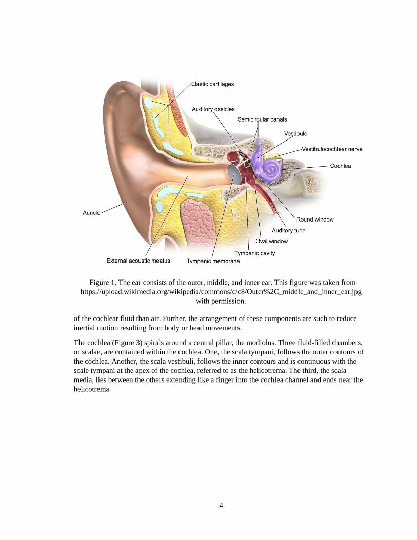
Sound pressure waves reaching the ear may be perceived. The ear consists of three parts: outer,
middle, and inner ear (Figure 1). The inner ear contains the cochlea, a spiral bony canal that is
filled with fluid. The cochlea also contains the organ of Corti, the sensory transduction apparatus.
Sound travels through the external ear canal, or external auditory meatus, continuing to the
middle ear (Figure 1). The pressure waves reaching the middle ear cause the tympanic membrane
to vibrate. This vibration is transferred through the middle ear to the inner ear by three small
bones (ossicles; Figure 2). A single ossicle, the malleus, is physically attached to the tympanic
membrane. The vibration is then transmitted to an opening in the cochlea, the oval window, by
the other two ossicles (the incus and stapes). This process is required to ensure efficient
transmission to the cochlea. Without this process, the sound would be reflected and not sensed
due to the higher acoustic impedance
4
Figure 1. The ear consists of the outer, middle, and inner ear. This figure was taken from
https://upload.wikimedia.org/wikipedia/commons/c/c8/Outer%2C_middle_and_inner_ear.jpg
with permission.
of the cochlear fluid than air. Further, the arrangement of these components are such to reduce
inertial motion resulting from body or head movements.
The cochlea (Figure 3) spirals around a central pillar, the modiolus. Three fluid-filled chambers,
or scalae, are contained within the cochlea. One, the scala tympani, follows the outer contours of
the cochlea. Another, the scala vestibuli, follows the inner contours and is continuous with the
scale tympani at the apex of the cochlea, referred to as the helicotrema. The third, the scala
media, lies between the others extending like a finger into the cochlea channel and ends near the
helicotrema.

5
Figure 2. The middle ear contains three small bones (ossicles) which transfers sound pressure
waves vibrating the tympanic membrane to an opening in the cochlea. This figure was taken with
permission from
https://commons.wikimedia.org/wiki/File:Blausen_0330_EarAnatomy_MiddleEar.png.

6
Figure 3. The cochlea contains the organ of Corti, the sensory transduction apparatus. The
cochlea contains three fluid-filled chambers which are used to transmit oscillations of the stapes.
This figure was taken with permission from
https://commons.wikimedia.org/wiki/File:1406_Cochlea.jpg.
Energy from the vibrating stapes is transmitted to the fluid in the scala vestibuli (perilymph). The
stapes pushes in and out of the cochlea as it oscillates, applying variable pressure on the
perilymph. The incompressible nature of the perilymph causes an alternating outward and inward
movement of the round window membrane of the scala tympani, located near the middle ear
cavity. The differential pressure between the scala vestibuli and scala tympani are converted into
oscillating movements of the fluid within scala media (endolymph). The movement of the
endolymph will stimulate movement of the basilar membrane in which the organ of Corti, the
sensory transducer in the scala media, rests. This movement results in slight vibrations in the
tectorial membrane of the organ of Corti. The differential movement between the tectorial and
basilar membranes excite and inhibit the sensory receptor cells in the organ of Corti.
The sensory receptor cells of the inner ear, residing in the organ of Corti, are called hair cells
(Figure 4). On the apical surface of each hair cell is a bundle of stereocilia, filled with stiff
parallel arrays of cross-bridged actin filaments. The stereocilia project into the overlying tectorial
membrane. The stereocilia will be displaced if the tectorial membrane and the basilar membrane
move with respect to one another. This occurs when the basilar membrane vibrates moving the
body of the hair cell causing the stereocilia to bend in relation to the hair cell body.
The motion of the stereocilia in one direction depolarizes the cell by opening K+ channels
producing an inward current (Figure 5). This inward current activates voltage-sensitive Ca2+ ion
channels. Motion in the opposite direction hyperpolarizes the cell by closing the K+ channels.
Thus, oscillations of the basilar membrane produce back-and-forth angular displacements of the
stereocilia resulting in sinusoidal potential changes at the frequency of the sound.

7
Figure 4. Hair cells reside in the organ of Corti. Hair cells are sensory receptors of the inner ear.
This figure was taken with permission from
https://commons.wikimedia.org/wiki/File:Gray931.png.
Figure 5. Motion of stereocilia can cause depolarization or hyperpolarization of hair cells by
opening or closing K+ channels. This figure was taken with permission from
https://commons.wikimedia.org/wiki/File:HairCell_Transduction.svg.
Hair cells also are capable of releasing chemical transmitters at their basal end. At the basal end,
hair cells are contacted by peripheral branches of bipolar neuron axons. A single auditory nerve

8
cell will only innervate a single inner hair cell. Each inner hair cell is innervated by
approximately 10 auditory nerves. Some auditory nerve fibers innervate many outer hair cells.
The cell bodies of these auditory neurons lie in the spiral ganglion and the central axons
constitute the auditory nerve. A neurotransmitter (glutamate) is released at the base of hair cells
when depolarized as a product of the increase in intracellular Ca2+, exciting the peripheral
terminal of the sensory neuron. Summation of sensory neuron excitation can result in action
potentials initiated in the auditory nerve cell’s central axon. The oscillation in the potential of the
hair cell causes oscillatory release of neurotransmitters and alternating the firing of axons in the
auditory nerve.
Auditory nerve cells enter the brain stem just under the cerebellum, and terminate in the cochlear
nucleus of the brain stem (Figure 6). Most axons of cochlear nucleus cells cross to the
contralateral side of the brain; the majority of auditory information processed by one half of the
brain comes from the ear on the opposite side of the head. Ventral cochlear nuclei project to the
superior olivary complex located in the brainstem. The superior olivary complex receives axons
that both cross and do not cross the midline. It is the first location in the ascending auditory
system which receives inputs from both ears (although the majority come from the contralateral
ear). Fibers leaving the superior olivary complex project along two pathways. Some synapse in
the nucleus of the lateral lemniscus while the majority travel to the inferior colliculus (IC)
directly. The central cochlear nuclei axons projecting to the superior olivary complex is thought
to play a role in localizing sound.
In contrast to the ventral pathway, dorsal cochlear nuclei project directly to the contralateral IC.
Both direct ventral and dorsal pathways to the IC are important in other aspects of auditory
perception. A major pathway in the IC allows information to cross the midline, enabling
information from both ears to be almost equally represented in both hemispheres of the brain in
further ascending pathways. Axons leaving the IC project to the medial geniculate nucleus
located in the thalamus. Medial geniculate fibers project to the primary auditory cortex (A1) in
the superior temporal gyrus (STG). Most cells within the auditory cortex receive input from both
ears. These cells are ordered in such a way that

9
Figure 6. Auditory nerve cells terminate in a small portion of the brain stem. This figure was
replicated with permission from https://commons.wikimedia.org/wiki/File:Gray691.png.
a relationship exists between the spatial position of the cells within the cortex and the frequencies
of sounds which they are sensitive. A1 is surrounded by higher order cortical auditory areas
located on both superior and lateral surfaces of the temporal lobe in the STG. The left cerebral
hemisphere, which has a longer lateral sulcus, is specialized for linguistic function and
interpretive speech mechanisms. The right hemisphere is involved in non-linguistic function such
as motor speech.
A1 contains several distinct tonotopic maps of the frequency spectrum. Different layers within the
auditory cortex form connections with other cortical areas and are functionally organized into
columns. Binaural cells are clustered into two alternating columnar groups, summation and
suppression columns, running from the pial surface to the underlying white matter. Summation

10
columns respond greater to binaural input than monaural while suppression columns respond the
greatest to monaural input. Functional divisions (Figure 7) in the frontal and temporal lobes are
utilized for the perception of speech sounds (Broca’s area and Wernicke’s area). Separate areas
are also utilized to map the timing, intensity, and frequency of the sound to generate a perception
of location, loudness, and pitch.
Figure 7. Different divisions of the frontal and temporal lobes are utilized in the perception of
sound. Angular Gyrus, orange; Supramarginal Gyrus, yellow; Broca’s area, blue; Wernicke’s
area, green; and A1, pink. This figure was replicated with permission from
https://commons.wikimedia.org/wiki/File:Brain_Surface_Gyri.SVG.
B. Tinnitus
There are two main categories of hearing loss. The first is caused by inner ear damage, usually
resulting in permanent deficits. The second results when sound waves do not traverse to the inner
ear, the effects of which are most likely reversible. In 2012, the World Health Organization
estimated 360 million people (5.3% of the world population) suffered from disabling hearing loss
(World Health Organization, 2012). Certain conditions such as age, illness, and genetics may
contribute to hearing loss, although the most common cause is repeated exposure to loud noises
(Vio & Holme, 2005). Noise-induced hearing loss is thought to cost between 0.2 and 2 percent
GDP (Vio & Holme, 2005).
Tinnitus, formally known as chronic subjective tinnitus, is the phantom perception of sound (e.g.
ringing, buzzing, roaring, clicking, or hissing): individuals perceive sound in the absence of a
physical sound wave. Tinnitus is not a condition itself but rather a symptom of an underlying
condition such as age-related hearing loss, ear injury, or a circulatory system disorder. Tinnitus is
one of the first signs of damage to the auditory system (Vio & Holme, 2005). The phantom noise
is highly variable in both pitch and intensity across individuals. Further, the phantom noise can
manifest itself laterally, appearing dominant in the left or right, or bilaterally, appearing as if
perceived both ears.

11
It has been reported that tinnitus affects 5-30% of the population (Axelsson & Ringdahl, 1989; de
Ridder et al., 2007; Fabijanska, Rogowski, Bartnik, & Skarzynski, 1999; Heller, 2003; Henry,
Dennis, & Schechter, 2005; Mühlnickel, Lutzenberger, & Flor, 1999; Vio & Holme, 2005;
Weissman & Hirsch, 2000; Wunderlich et al., 2010). In a recent study by the U.S. Centers for
Disease Control, 7.3% of the 9364 people questioned reported they have been bothered by
ringing, roaring, or buzzing for more than five minutes within the previous year. 41.4% of these
individuals reported the ringing, roaring, or buzzing has been perceived for more than five years,
and 67.3% reported more than one year (U.S. Centers for Disease Control, 2013).
It was previously reported that 6-25% report interference with their daily lives causing
considerable distress (Baguley, 2002; Eggermont & Roberts, 2004; Heller, 2003; Smits et al.,
2007), and that tinnitus causes severe disabilities in 0.2-1% of the population which restrict the
performance of daily functions (Andersson & Kaldo, 2004; Axelsson & Ringdahl, 1989; Coles,
1984; Davis & Rafaie, 2000; de Ridder et al., 2007; Leske, 1981; Meyershoff, 1992; Mühlnickel
et al., 1999; Vio & Holme, 2005). From the same U.S. Centers for Disease Control study, 16.8%
of those reporting a tinnitus percept indicated that it was bothersome. Further, 3.3% classified the
tinnitus percept as being a very big problem, and 30.6% indicated it was a moderate problem or
worse (U.S. Centers for Disease Control, 2013). An American Tinnitus Association report
suggests approximately 20 million people are dealing with burdensome tinnitus on a regular
basis. More importantly, nearly 2 million people struggle with severe, potentially debilitating,
tinnitus (American Tinnitus Association, 2015).
In the majority of tinnitus cases, there is no obvious source (i.e. blood vessel problems, an inner
ear bone condition, or muscle contractions) for the phantom sound (Fowler, 1944; Penner, 1990;
Sismanis & Smoker, 1994). It can interfere with everyday tasks by decreasing concentration or
interfering with the perception of actual sound. Furthermore, individuals affected by tinnitus may
also experience fatigue, stress, sleep problems, memory problems, depression, anxiety, and
irritability (Vanneste et al., 2010). Interestingly, psychometric quantities cannot accurately predict
the distress one may encounter (Golm, Schmidt-Samoa, Dechent, & Kröner-Herwig, 2013). The
Neurophysiological Model (Jastreboff, Gray, & Gold, 1996) proposes distress emerges if initial
perception is associated with a negative evaluation.
In the U.S. military, tinnitus is the number one service-connected disability in Gulf War Era
(1990 – present) veterans. In 2014, almost half of new compensation recipients of service-
connected disability payments had tinnitus, and almost 1.3 million veterans received
compensation for service-connected tinnitus disability. This was the most prevalent disability
among new compensation recipients and all recipients, with more than 300,000 more cases than
hearing loss and more than 500,000 cases than post-traumatic stress disorder. Almost half of new
and a third of total compensation recipients receive disability for tinnitus, representing 9.5% and
7.2% of total disabilities, respectively. Both proportions are higher than any other disability. With
an average annual payout of $13,732, service-connected tinnitus disability payments are
estimated at $3.9 billion. Although the average recipient has 4.5 disabilities (U.S. Department of
Veterans Affairs, 2014), the cost due solely to tinnitus is difficult to determine. The delivery of
tinnitus-related healthcare services to these individuals is estimated to be much higher (American
Tinnitus Association, 2015). In summation, tinnitus has a major impact in the effectiveness of the
U.S. military, from personnel issues to degraded mission success rates caused by lower situational
12
awareness or reduced performance (Hearing Center of Excellence, 2013), and major economic
and social impacts.
C. Biomarkers of Tinnitus
The neural underpinnings of tinnitus are currently unknown. With tinnitus being a symptom of an
underlying condition, it is difficult to study and isolate the causes and effects due to tinnitus.
However, evidence supports a central mechanism for the tinnitus percept, as it remains following
complete dissection of the auditory nerve (Folmer, Griest, & Martin, 2001). In the following
sections, the current state of the art in the study of tinnitus using MR methods will be presented.
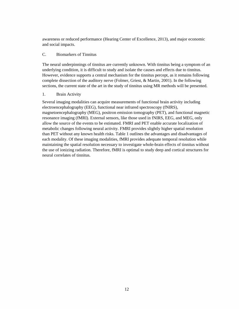
1. Brain Activity
Several imaging modalities can acquire measurements of functional brain activity including
electroencephalography (EEG), functional near infrared spectroscopy (fNIRS),
magnetoencephalography (MEG), positron emission tomography (PET), and functional magnetic
resonance imaging (fMRI). External sensors, like those used in fNIRS, EEG, and MEG, only
allow the source of the events to be estimated. FMRI and PET enable accurate localization of
metabolic changes following neural activity. FMRI provides slightly higher spatial resolution
than PET without any known health risks. Table 1 outlines the advantages and disadvantages of
each modality. Of these imaging modalities, fMRI provides adequate temporal resolution while
maintaining the spatial resolution necessary to investigate whole-brain effects of tinnitus without
the use of ionizing radiation. Therefore, fMRI is optimal to study deep and cortical structures for
neural correlates of tinnitus.

13
Table 1. Advantages and disadvantages of functional brain imaging modalities.
Technology Advantages Disadvantages
Magnetoencephalography
• Direct measure of neural
activity
• Non-invasive
• No side effects
• Expensive
• Low availability
• Low spatial resolution
• Limited to cortical activity
Positron Emission
Tomography • High spatial resolution
• Requires radioactive
nuclei
• Low temporal resolution
• High cost
• Indirect measure of neural
activity
Electroencephalography
• Direct measure of neural
activity
• High temporal resolution
• Low cost
• Non-invasive
• No side effects
• Small signal-to-noise ratio
• Low spatial resolution
• Signal can contain
artifacts from muscle
activity, eye movements,
and blinking
• Long set-up time
Functional Magnetic
Resonance Imaging
• High spatial resolution
• No side effects
• Non-invasive
• High cost
• Low temporal resolution
• Indirect measure of neural
activity
Functional Near-Infrared
Spectroscopy
• High temporal resolution
• Non-invasive
• No side effects
• Low cost
• Low spatial resolution
• Indirect measure of neural
activity
a. Background on Functional Magnetic Resonance Imaging
i. Physics
FMRI was developed from nuclear magnetic resonance (NMR). NMR exploits the magnetic
properties of atomic nuclei to measure signals from protons and neutrons of atomic nuclei.
Protons and neutrons possess an intrinsic angular momentum referred to as the “spin”. This
angular momentum cannot be changed, but the axis of spin can be manipulated. When a nucleus
has an even number of protons and neutrons, the nucleus has no net spin and is not magnetic (i.e.
cannot be detected using NMR). However, when a nucleus has an odd number, there is a net spin
and NMR can be used to alter the spins.
Along with an angular momentum, each spin has a magnetic dipole moment. This allows a
magnetic field to exert a torque on protons capable of rotating the dipole into alignment with the
field. During this rotation, the angular moment causes the spins to precess around the field axis.
The frequency of precession, referred to as the Larmor frequency, is unique to every atom. This
frequency is directly proportional to the strength of the magnetic field:
𝜔 = −𝛾𝛽0 ( 2 )
where β0 is the strength of the magnetic field and γ is the magnetogyro ratio represented as a
function of the magnetic moment µ and spin angular momentum J:
14
𝛾 = 𝜇/𝐽. ( 3 )
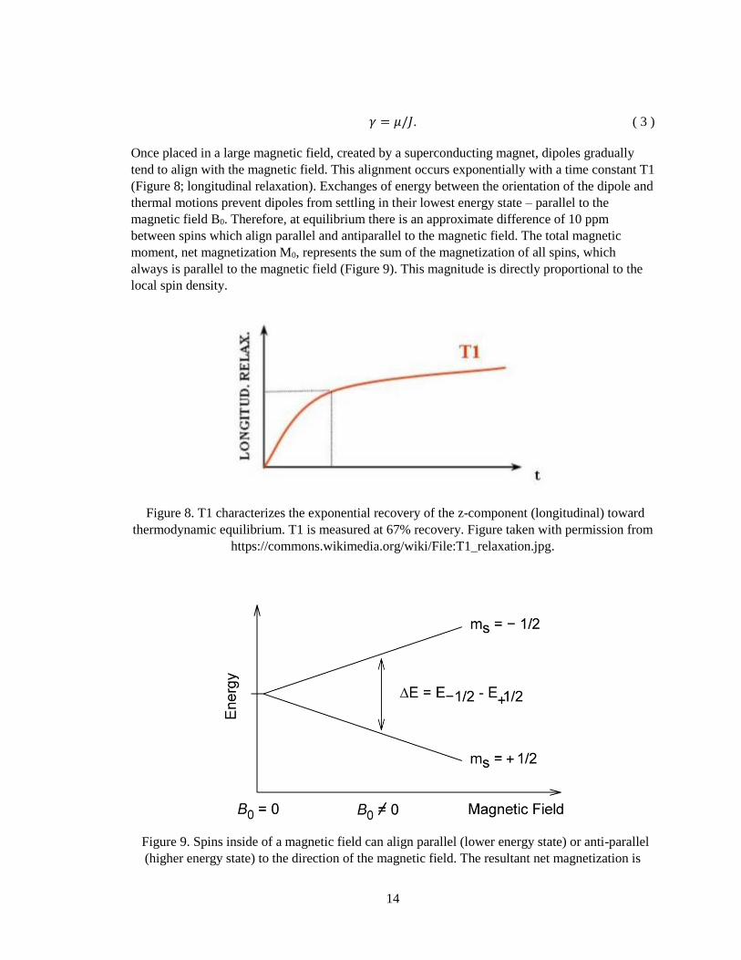
Once placed in a large magnetic field, created by a superconducting magnet, dipoles gradually
tend to align with the magnetic field. This alignment occurs exponentially with a time constant T1
(Figure 8; longitudinal relaxation). Exchanges of energy between the orientation of the dipole and
thermal motions prevent dipoles from settling in their lowest energy state – parallel to the
magnetic field B0. Therefore, at equilibrium there is an approximate difference of 10 ppm
between spins which align parallel and antiparallel to the magnetic field. The total magnetic
moment, net magnetization M0, represents the sum of the magnetization of all spins, which
always is parallel to the magnetic field (Figure 9). This magnitude is directly proportional to the
local spin density.
Figure 8. T1 characterizes the exponential recovery of the z-component (longitudinal) toward
thermodynamic equilibrium. T1 is measured at 67% recovery. Figure taken with permission from
https://commons.wikimedia.org/wiki/File:T1_relaxation.jpg.
Figure 9. Spins inside of a magnetic field can align parallel (lower energy state) or anti-parallel
(higher energy state) to the direction of the magnetic field. The resultant net magnetization is

15
aligned with the magnetic field. This figure was replication with permission from
https://commons.wikimedia.org/wiki/File:NMR_splitting.gif.
A measurable, transient signal can be produced by using a radiofrequency (RF) pulse to tip the
dipoles which contribute to M0. The RF pulse is delivered by passing a current through a coil
perpendicular to the magnetic field. The RF pulse sends electromagnetic waves which resonate at
particular frequencies. These pulses perturb the equilibrium state which exists inside the magnetic
field. A specific RF can be selected to match a Larmor frequency to excite specific spins. The
target spins absorb the energy in the electromagnetic wave, energy that is released when the RF
pulse is turned off. Current is induced from the energy released from the excited spins in the coils
which produce the RF pulse. The measured current is proportional to the magnitude of the
precessing magnetization. Once the RF pulse ends, the net precession magnetization decays
exponentially with a time constant T2 (Figure 10; transverse relaxation). This delay occurs as the
phase between precessions across spins increases and no longer add coherently. Both T1 and T2
vary between tissue types, developing contrast between various tissues in the constructed images.
Figure 10. T2 characterizes the exponential decay of the transverse component of the
magnetization vector, measured at 37%. Figure taken with permission from
https://commons.wikimedia.org/wiki/File:T2_relaxation.svg.
Images can be created by applying gradients to the magnetic field. Three orthogonal coils are
used to create linear gradients in each dimension. Equation 2 specifies the resonant frequency of
protons is directly proportional to the magnetic field. Therefore, once a gradient is created,
protons in different spatial locations will resonate at different frequencies. The strength of these
gradients are small compared to B0, and are usually expressed in units of the resonant frequency
change they produce per unit length (cm). RF pulses are shaped to produce only a narrow band of
frequencies centered on a particular frequency. Only the protons resonating within this band will
be excited by the RF pulse, and these protons should reside in a specific, known slice relative to
the magnetic field gradient (Figure 11). Information can be encoded about the remaining two
dimensions of each signal allowing the image of the distribution in this plane to be reconstructed
(Buxton, 2009; Hendee & Ritenour, 2002; Huettel, Song, & McCarthy, 2004).

16
Figure 11. Gradients in the magnetic field cause the frequency of precession to vary throughout
the field. The input RF frequency can be tuned to target spins from a specific location in the
gradient field and, therefore, specific spatial locations. This figure was taken from with
permission from
https://commons.wikimedia.org/wiki/File:Tomographic_imaging_slice_selection.jpg.
ii. Neurophysiology
The physical laws of thermodynamics state any chemical system that is not at equilibrium has the
capacity to do “work”. The capacity is called the free energy of the system. Neurons at steady-
state are not in equilibrium due to an imbalance between intra- and extra-cellular ionic
concentrations and, therefore, have the ability to do work. This work is referred to as an action
potential: the opening and closing of ion channels along the axon which produces a current along
the cell membrane and the release of neurotransmitters at the synapse. The available free energy
of neurons is reduced with each action potential and neurotransmitter release. Energy metabolism
is required to restore the free energy and return the neuron to its state prior to the action potential.
This process involves the conversion of adenosine triphosphate (ATP) to adenosine diphosphate
(ADP) coupled to other reactions referred to as ATPase (Buxton, 2009). Glucose and oxygen are
used to restore the ATP/ADP ratio following the free energy recovery.
The mechanism for free energy recovery from glucose and oxygen is completed in four stages. In
the first stage, glycolysis, glucose is broken down into two pyruvate molecules. Next, the citric
acid cycle (Kreb’s cycle) breaks pyruvate down to form carbon dioxide in the mitochondria.
Energy is stored in the form of reduced nicotinamide adenine dinucleotide (NADH). In the third
stage, the electron transfer chain in the mitochondria transfers electrons from NADH to oxygen to
form water. Coupled with this is the pumping of H+ across the inner membrane of mitochondria
against is gradient, thus storing energy. The final stage moves H+ across the gradient coupled
with the combination of ADP and pyruvate form ATP. The product of this metabolism is carbon
dioxide and heat, which is carried away by venous blood.
The human brain requires a high level of energy metabolism. To fuel the brain, it is supplied with
approximately 15% of total cardiac output (Buxton, 2009). Blood flow is used to deliver glucose
and oxygen to the brain, which requires a continuous supply of glucose and oxygen as it contains
virtually no reserve storage of oxygen. Glucose diffuses out of the blood down its gradient
through channels in the capillary wall. Directional preference does not exist for these channels;
therefore, this method is also used to return unmetabolized glucose to the blood stream. Glucose

17
is delivered in excess to the required amount at rest. Approximately 15% of glucose delivered to
the capillary bed is metabolized (Buxton, 2009).
Oxygen, however, is carried in the blood by hemoglobin but a small fraction exists as dissolved
gas in the plasma. Oxygen is transported down a concentration gradient between dissolved gas in
capillary plasma and dissolved gas in tissue. When oxygen diffuses out of the capillary it is
replenished by the release of oxygen bound to hemoglobin, or oxyhemoglobin. Hemoglobin
which loses the oxygen it carries becomes deoxyhemoglobin, and the magnetic properties change
in a subtle way. These changes alter the NMR signal slightly: the magnitude of the signal from
protons within oxyhemoglobin is slightly higher than that from deoxyhemoglobin. When an area
of the brain becomes active, blood flow to this area increases much more than the oxygen
metabolic rate leading to a reduction in the oxygen extraction fraction – the fraction of oxygen
leaving the blood and metabolized in cells. These two phenomena sum to create local, measurable
increases in the NMR signal called the blood oxygen-level dependent (BOLD) effect. The
hemodynamic response function (HRF) describes how the BOLD effect responds to neural
activation (Figure 12).
Figure 12. Group average HRFs. HRFs were the averaged BOLD signal from the 10 voxels
which responded most robustly to a flashing monochrome checkerboard stimulus. The HRFs
were then averaged across individuals and trials. The blue line indicates children (aged 7 to 20),
the green line indicates young adults (aged 21 to 27), and the yellow line indicated older adults
(aged 30+). Reprinted from Richter and Richter (2003) with permission from Elsevier.
The classical understanding of the relationship between neural activity and changes in blood flow
is described with a chain of events. First, neural activity increases the local rate of energy
metabolism. To fuel the metabolism, blood flow must be increased to deliver glucose and oxygen
to the active area. However, recent views seem to contradict this classical theory. New principles
hypothesize changes in blood flow are driven directly by aspects of neuronal activity. Multiple
neuronal signaling pathways seem to drive modifications of blood flow. Astrocytes, which make
contact with blood vessels and neurons, have a complex signaling method and may create a
bridge between neuronal signaling and changes in blood flow. Therefore, these astrocytes may
play an important role in driving changes in blood flow following neural activity (Buxton, 2009).
In either case, changes in blood flow are a correlate of neural activity.

18
b. FMRI-based Correlates of Tinnitus
A growing theory, the Global Brain Model (Schlee et al., 2011), builds upon the
Neurophysiological Model describing tinnitus as a result from abnormal brain activity arising at
points along the auditory pathway. Reduced sensory input due to a damaged hearing system
decreases inhibitory mechanisms in the central auditory system and enhances excitability of the
auditory cortices. This aberrant activity creates the perception of a sound although no sound is
present (Eggermont & Roberts, 2004; Giraud et al., 1999; Jastreboff, 1990). Such neural
correlates of tinnitus may arise due to neuroplastic mechanisms engaged in response to total or
partial deafferentation somewhere in the auditory tract (de Ridder et al., 2004; Kaltenbach, 2000;
Mühlnickel, Elbert, Taub, & Flor, 1998). It has been suggested that these changes may be driven
by a compensatory mechanism to enhance excitability of auditory cortices in response to reduced
sensory input caused by damage to the mechanical system of the ear (Golm et al., 2013).
i. Assessment of Tinnitus from Continuous Noise Stimulation
In most individuals, the tinnitus percept can be masked by an acoustic stimulus (Feldmann, 1971;
Fowler, 1944; Penner, Brauth, & Hood, 1981). Melcher, Sigalovsky, Guinan, & Levine. (2000)
proposed auditory stimulation (continuous, broadband noise) in a block design1 will alternate the
loudness of the tinnitus percept, thus revealing tinnitus-related abnormalities. Participants were
separated into subpopulations experiencing either lateralized or non-lateralized tinnitus, and
compared to a group of healthy individuals who do not have tinnitus or whose tinnitus was
masked completely by the acoustic noise in the imaging environment. Four of the thirteen
participants had some hearing loss, two from the non-lateralized group and two from the healthy
controls. Auditory stimulation was performed binaurally or monaurally, dependent upon the run,
at 55 dB sensation level, established inside the MRI, except in the first four experiments which
used 35, 40, or 60 dB. The noise was alternated with periods with no stimulation. Activity in the
IC was assessed using fMRI. IC activity did not significantly vary between the control and non-
lateralized groups, and were grouped into a single reference group. For this reference group,
binaural noise produced comparable levels of activation in the left and right IC. In lateralized
tinnitus participants, binaural noise produced abnormally low activation in the IC contralateral to
the tinnitus percept. Activity in the IC ipsilateral to the tinnitus percept did not significantly vary
from the reference group. Monaural noise produced greater activation in the IC contralateral to
the stimulus in the reference group. Left stimulation in the IC contralateral to the tinnitus percept
resulted in decreased activity in the lateralized tinnitus group than the reference group. Further,
activation in the left IC for right stimulation was less than activation in the right IC for left
stimulation for all lateralized tinnitus participants. These phenomena only appeared in 2 of the 6
in the reference participants.
Gu, Halpin, Nam, Levine, & Melcher (2010) explained that hyperacusis, increased perception of
sound loudness, can accompany tinnitus. Hyperacusis, like tinnitus, is thought to arise from
abnormal gain in the auditory pathway (Levine & Kiang, 1995; Salvi, Wang, & Ding, 2000).
They suggest that hyperacusis must be controlled in the experimental population to determine if
1 In block design experiments, two or more conditions are alternated in distinct blocks only useful for
determining which voxels show differential signals between conditions.

19
the previously observed abnormal activity (e.g. Melcher et al., 2000) were attributable solely to
tinnitus. In their study, sound-level tolerance (SLT) was measured from each participant to
address whether tinnitus, abnormal SLT, or both contribute to aberrant brain activity. During
fMRI acquisition broadband noise was delivered binaurally at 50, 70, and 80 dB sound pressure
level alternated periods of no auditory stimulation. Their region of interest (ROI) based analysis
revealed elevated activity in the auditory midbrain, thalamus, and A1 in participants with
hyperacusis. They did not report any subcortical region with abnormal activity in participants
with tinnitus, however, elevated activity in A1 was observed. This elevated activity was more
prominent with the 50 dB stimulation than the 70 dB. The lack of subcortical hyperactivity in
tinnitus patients leads to the hypothesis that elevations of activity in cortical structures (e.g. A1)
may be driven by attention drawn to the auditory system as subcortical activity is less likely
modulated by attentional state, although their analysis did not include any attentional regions
which could have supported this theory.
Seydell-Greenwald et al. (2012) add to this body of research. Their study involved auditory
stimulation of tinnitus patients and age/sex matched controls. Binaural stimulation consisted of
trains of short noise bursts centered around 375, 1500, and 6000 Hz. For each tinnitus patient, the
noise nearest the tinnitus frequency, determined through subjective pitch and tone matching, was
replaced with a stimulus centered at the tinnitus frequency. Stimuli were delivered at a constant
level 15 to 30 dB above SLT, determined inside the scanner, depending upon the highest intensity
that did not induce sound artifacts. In a whole-brain analysis, two clusters were identified with a
significant group difference between tinnitus patients and healthy controls for trials with
stimulation at the tinnitus frequency compared to trials without auditory stimulation. These
clusters were centered in the right ventro-medial prefrontal cortex (vmPFC) and right STG. They
did not find any significant group differences with stimulation of frequencies which were not near
the tinnitus frequency compared to trials without auditory stimulation. For the group of tinnitus
patients, the BOLD response in the vmPFC was strongly correlated with subjective measures of
tinnitus: general loudness ratings and tinnitus awareness. These correlations were strongest on
trials with stimulation at the tinnitus frequency. They propose the vmPFC provides input for a
thalamic auditory gating mechanism that can suppress the tinnitus percept. Tinnitus patients
likely engaged their inhibitory gating mechanism to drive attention away from the tinnitus percept
while control participants were not likely engaging this system.
ii. Other Methods to Assess Tinnitus-related Abnormalities
Alternative methods have been proposed for the investigation of tinnitus-related abnormalities in
brain activity. These methods are based upon assessing the interaction between activity and
external stimuli such as sound, instead of the aforementioned method which attempts to alter the
tinnitus percept. Smits, Kovacs, de Ridder, Peeters, van Hecke, & Sunaert (2007) binaurally
presented lyrical pop music to lateralized and non-lateralized tinnitus patients in addition to
healthy volunteers. Asymmetrical activation was observed in the auditory cortices (A1, IC, and
medial geniculate body) in patients with lateralized tinnitus, with reduced activity in cortices
contralateral to the tinnitus percept. Although it is possible the stimuli masked the tinnitus percept
which could lead to lower activity on the affected side. For those with non-lateralized tinnitus this
activation was symmetrical. Activation was also symmetrical for healthy controls for auditory
cortices, except A1 which was left-lateralized as anticipated for linguistic and nonlinguistic

20
stimuli. The researchers suggest this indicates increased spontaneous activity of the affected brain
areas in tinnitus patients during rest.
Wunderlich et al. (2010) recruited tinnitus patients and healthy controls to perform a pitch
discrimination task. Activation in the caudate nucleus, superior frontal gyrus, and cingulate cortex
was increased in the tinnitus patients when compared to healthy controls. This suggests tinnitus
enhances the emotional response to auditory stimuli. Using the theory that distress heightens
tinnitus perception and attentional focus on the percept, Golm, Schmidt-Samoa, Dechent, &
Kröner-Herwig (2013) used an emotional sentence task to evaluate high- and low-distressed
tinnitus patients in addition to healthy controls. High-distressed tinnitus patients showed stronger
activity compared to healthy controls in parts of the cingulate gyrus, insula, dorsolateral
prefrontal cortex, orbitofrontal cortex, and left middle frontal gyrus when contrasting tinnitus-
related sentences to neutral ones. Activity in the left middle frontal gyrus was also enhanced in
the high-distressed group compared with the low-distressed. Correlations between a seed region
of the left middle frontal gyrus and limbic, frontal, and parietal regions were stronger for the
high-distressed group.
iii. Summary
Several different paradigms utilizing various designs have reported variations between healthy
individuals and those affected by tinnitus. This evidence supports a central mechanism for the
tinnitus percept and not the subcortical structures originally identified, but suggests this effect
further extends to areas involved in the processing of emotion and attentional state. Variations in
activity between tinnitus patients and healthy counterparts were described. Also, differences in
lateralized and non-lateralized tinnitus patients as well as between low- and high-distressed
groups were reported.
2. Resting-State Networks
Neural networks can be described in two ways: anatomical and functional. Anatomical networks
define the physical connections between brain regions made by single axons or white matter
tracts. In contrast, functional networks are defined by the interactions between brain regions in
the execution of cognitive functions. The fundamental principle of functional connectivity is that
individual regions within the network have activity which temporally co-vary, allowing for
emergent functions and cognitive processing (Guo & Blumenfeld, 2014).
a. Background on Resting-State fMRI
Functional networks are characterized by systematic, spontaneous low-frequency (<0.1 Hz)
signal fluctuations (SLFs). SLFs from regions which are functionally connected appear to
fluctuate synchronously. FMRI is well-suited to derive measures functional connectivity given its
good spatial resolution and temporal resolution fair enough to capture SLFs. In traditional fMRI,
specific variables are intentionally modulated to detect corresponding changes in the measured
BOLD signal. To detect SLFs, fMRI data is acquired when individuals are at rest (i.e. resting-
state fMRI), diverging from the traditional methods of fMRI. Biswal, Zerrin Yetkin, Haughton, &
Hyde (1995) first applied resting-state fMRI to study functional connectivity in individuals at
rest. They found a high degree of correlation between SLFs of regions associated with motor
function. This is the first demonstration that SLFs measured at rest from functionally-related
regions are correlated and detectable by fMRI.

21
Biswal et al. (1995) used a seed region in the left somatosensory cortex to derive correlation
coefficients, which defined the measure of functional connectivity. In this type of analysis, a seed
region is selected by the researcher and correlations between the time-course of this seed region
and other regions (or voxels) is computed. This approach is straightforward, but is highly
susceptible to bias as the results are dependent upon the chosen seed regions. In comparison,
independent component analyses (ICAs) are primarily data driven and, therefore, do not require a
priori hypotheses. In this method, components are produced from the time-courses. Common
components across voxels represent regions with common temporal covariation. However, the
results from an ICA approach are not as straightforward to interpret at the seed region approach
but are less susceptible to bias.
b. Resting-State fMRI Correlates of Tinnitus
FMRI studies indicate that the persistence of this phantom perception is associated with interplay
between the auditory and cognitive-emotional brain networks (see Section II.C.1.b above). This
disruption causes impariement in subsequent conditioned emotional reactions to tinnitus (Mirz et
al., 1999; Wunderlich et al., 2010). The use of a diverse set of networks to perform auditory
processing has been shown in normal hearing, healthy adults (Langers & Melcher, 2011).
Evidence of these plastic changes suggests the possible functional reorganization of the networks
which exist between auditory and cognitive-emotional brain regions, changes which may
correlate with the appearance of tinnitus.
i. Assessment of Functional Connectivity from Resting-State fMRI
Subjective tinnitus2 can easily be studied using resting-state fMRI where it is not necessary to
perform task-based modulations, although this is possible (see Section II.C.1.b above). However,
it may be plausible that the continuous perception of a chronic internal noise restricts an
individual from truly achieving a resting state; they may be in a continuous task-based state. This
steady task-based state is thought to be cause detectable alterations in networks, such as the
default mode network (DMN), when compared to healthy humans. Contrary to other networks,
the DMN shows enhanced activity at rest and reduced activity when individuals enter a task-
based state (Shulman et al., 1997). Therefore, it would be expected to observe reduced DMN in
tinnitus patients compared to healthy controls.
Kim et al. (2012) conducted one of the first studies to investigate altered functional connectivity
in tinnitus patients using fMRI. They compared connectivity of auditory cortices from four
patients to six age-matched healthy controls. Using an ICA approach, they found increased
connectivity between the auditory cortex and the limbic system in tinnitus patients. This supports
Gu et al.’s (2010) postulation that elevated A1 activity may be driven by attention drawn to the
auditory. In a ROI analysis, correlations were computed between four seed regions comprised of
the left and right primary and secondary auditory cortices. Connectivity scores were computed
from each of these regions. They identified a decreased connectivity between left and right
2 This project will only consider subjective tinnitus, a form of tinnitus where the cause of the tinnitus
percept cannot be linked to something physical. In the few cases where the tinnitus percept can be
objectively heard by others (e.g. through the use of a stethoscope), the phantom sound arises from a
physical phenomenon (e.g. muscle contractions, blood flow).

22
auditory cortical regions. Further, they revealed increased connectivity in the left amygdala and
the dorsomedial prefrontal cortex in tinnitus patients compared to healthy controls. Their
evidence suggests elevated intrinsic brain connectivity between auditory networks and regions
involved in emotion processing and cognitive control. Additionally, their evidence supports the
hypothesis that tinnitus may be related to a reduction in the balance of excitatory and inhibitory
inputs to the central auditory system. This imbalance is observed through the reduced
interhemispheric coherence, where equilibrium is important for optimal function (Diesch,
Andermann, Flor, & Rupp, 2010).
Maudoux et al. (2012) compared resting-state functional connectivity, measured from fMRI, on
two groups. They selected auditory ROIs from the first group of twelve healthy individuals. Data
from a second group of thirteen patients with chronic tinnitus was compared to the first group. In
the second group, patients with hyperacusis and phonophobia were excluded. The identified
auditory network in healthy controls included bilateral primary and associative auditory cortices,
insula, prefrontal, sensorimotor, anterior cingulate (ACC), and left occipital cortices. The group
of tinnitus patients showed a similar network, excluding the ACC. In this group, the identified
auditory network also included regions of the brainstem, thalamus, nucleus accumbens, isthmus
of cingulate gyrus, right occipital, parietal, and prefrontal cortices. Further, for the tinnitus
patients, increased connectivity was identified in deeper brain structures (brainstem, cerebellum,
right basal ganglia/nucleus accumbens), right frontal and parietal, and left sensorimotor and
superior temporal regions. Finally, the tinnitus patients showed lower connectivity in the right
A1, left fusiform gyrus, and left frontal and bilateral occipital regions.
Davies, Gander, Andrews, & Hall (2014) conducted a comparison of resting-state functional
connectivity between twelve tinnitus patients and eleven age-matched healthy controls. Resting-
state fMRI were collected and analyzed using ICA to extract auditory components of interest. In
an ROI analysis, similar to Kim et al. (2012), when corrected for family-wise error the two
groups did not appear to have differences in functional connectivity. This study contradicts earlier
reports of disturbed connectivity (Kim et al., 2012; Maudoux et al., 2012), however this may be
due to methodological differences. Tinnitus symptoms are variable (e.g. lateralized, non-
lateralized) and is often accompanied by other disorders such as hearing loss. While Kim et al.
(2012) studied patients with lateralized tinnitus, Davies et al. (2014) used a cohort of patients
experiencing bilateral tinnitus. Further, Kim et al. (2012) did not account for high frequency
hearing loss in their control group while Davies et al. (2014) did.
ii. Summary
Few studies have explored tinnitus physiopathology through resting-state functional connectivity
using fMRI. The results from two studies suggested detectable differences in resting-state
functional connectivity, aligning with the Neurophysiological Model which suggests non-auditory
tinnitus physiopathology. Both of these studies indicated increased input from the limbic system
which coincide with postulations made in previous auditory stimulation fMRI studies. This effect
is proposed in the Neurophysiological Model, suggesting the limbic system plays a role in
negative reinforcement and draws more attention to the auditory system causing the tinnitus
signal to be perceived. Furthermore, these studies indicate altered connectivity in the nucleus
accumbens and associated paralimbic regions in the medial prefrontal cortex when compared to
healthy controls. These regions have been implicated to play a role in an inhibitory feedback loop
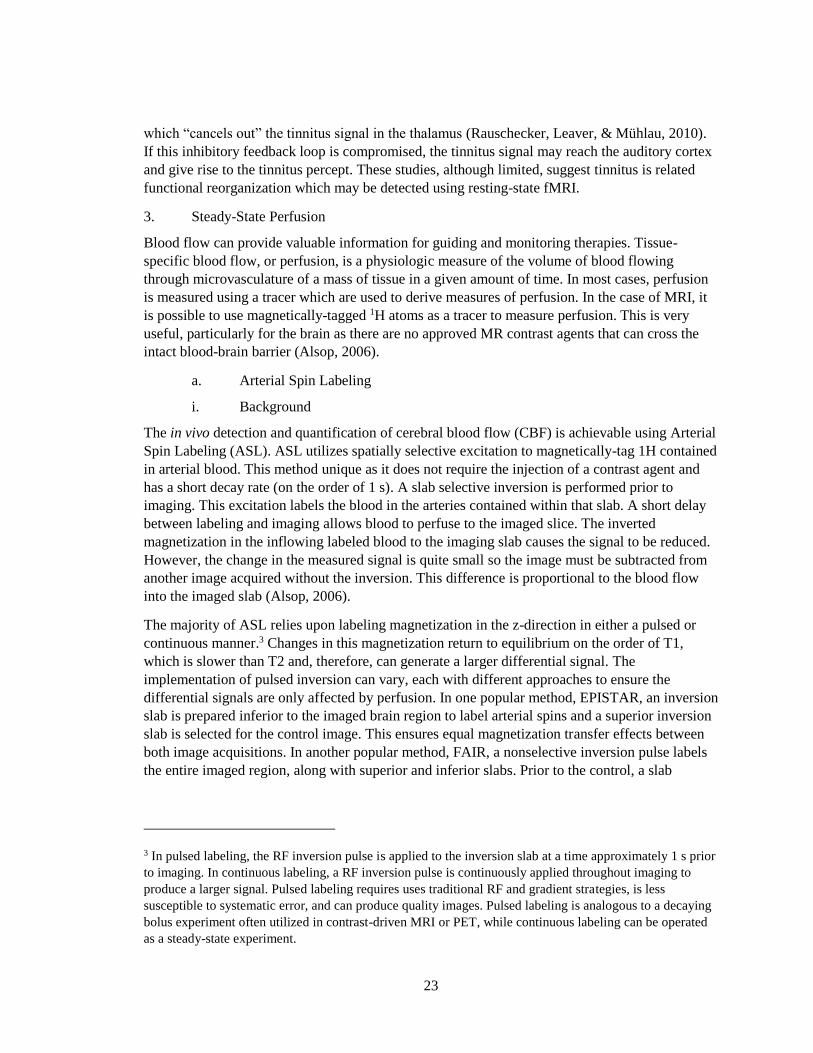
23
which “cancels out” the tinnitus signal in the thalamus (Rauschecker, Leaver, & Mühlau, 2010).
If this inhibitory feedback loop is compromised, the tinnitus signal may reach the auditory cortex
and give rise to the tinnitus percept. These studies, although limited, suggest tinnitus is related
functional reorganization which may be detected using resting-state fMRI.
3. Steady-State Perfusion
Blood flow can provide valuable information for guiding and monitoring therapies. Tissue-
specific blood flow, or perfusion, is a physiologic measure of the volume of blood flowing
through microvasculature of a mass of tissue in a given amount of time. In most cases, perfusion
is measured using a tracer which are used to derive measures of perfusion. In the case of MRI, it
is possible to use magnetically-tagged 1H atoms as a tracer to measure perfusion. This is very
useful, particularly for the brain as there are no approved MR contrast agents that can cross the
intact blood-brain barrier (Alsop, 2006).
a. Arterial Spin Labeling
i. Background
The in vivo detection and quantification of cerebral blood flow (CBF) is achievable using Arterial
Spin Labeling (ASL). ASL utilizes spatially selective excitation to magnetically-tag 1H contained
in arterial blood. This method unique as it does not require the injection of a contrast agent and
has a short decay rate (on the order of 1 s). A slab selective inversion is performed prior to
imaging. This excitation labels the blood in the arteries contained within that slab. A short delay
between labeling and imaging allows blood to perfuse to the imaged slice. The inverted
magnetization in the inflowing labeled blood to the imaging slab causes the signal to be reduced.
However, the change in the measured signal is quite small so the image must be subtracted from
another image acquired without the inversion. This difference is proportional to the blood flow
into the imaged slab (Alsop, 2006).
The majority of ASL relies upon labeling magnetization in the z-direction in either a pulsed or
continuous manner.3 Changes in this magnetization return to equilibrium on the order of T1,
which is slower than T2 and, therefore, can generate a larger differential signal. The
implementation of pulsed inversion can vary, each with different approaches to ensure the
differential signals are only affected by perfusion. In one popular method, EPISTAR, an inversion
slab is prepared inferior to the imaged brain region to label arterial spins and a superior inversion
slab is selected for the control image. This ensures equal magnetization transfer effects between
both image acquisitions. In another popular method, FAIR, a nonselective inversion pulse labels
the entire imaged region, along with superior and inferior slabs. Prior to the control, a slab
3 In pulsed labeling, the RF inversion pulse is applied to the inversion slab at a time approximately 1 s prior
to imaging. In continuous labeling, a RF inversion pulse is continuously applied throughout imaging to
produce a larger signal. Pulsed labeling requires uses traditional RF and gradient strategies, is less
susceptible to systematic error, and can produce quality images. Pulsed labeling is analogous to a decaying
bolus experiment often utilized in contrast-driven MRI or PET, while continuous labeling can be operated
as a steady-state experiment.

24
selective inversion is applied to only the entire imaged region. In this technique, the spins are
always inverted rather than left unaffected in the control as in the EPISTAR method.
ii. Quantification of CBF
The simple subtraction image from ASL is reflective of relative blood flow but quantitative
measurements can be very useful, specifically in clinical applications. Magnetization in the z-
direction behaves according to the Bloch equation, assuming no flow or RF pulses:
𝜕𝑀𝑧
𝜕𝑡 = −
𝑀𝑧−𝑀𝑧0
𝑇1, ( 4 )
where Mz represents the net magnetization in the z-direction at time t and M0z represents the net
magnetization in the z-direction at time 0. When blood flow occurs, inflowing spins from arteries
add their magnetization to the voxel and magnetization from outflowing spins subtract from the
voxel. The Bloch equation can be modified to account for flow:
𝜕𝑀𝑧
𝜕𝑡 = −
𝑀𝑧−𝑀𝑧0
𝑇1+ 𝜌𝑏𝑓(𝑀𝑎 − 𝑀𝑣), ( 5 )
where f is the blood flow (perfusion), ρb is the tissue density, Ma is the magnetization in the
inflowing spins, and Mv is the magnetization in outflowing spins. One can assume complete free
diffusion into the tissue, meaning Mv equals Mz at the capillary level.
From the flow-modified Bloch equation, it is apparent the ASL signal represents a competition
between T1 decay and inflow of labeled spins. Using this modified equation, the image intensity
due to ASL is approximately f*T1. The T1 decay of blood is often taken from literature, but
attempts have been made to measure it in vivo. Also, T1 of tissue can vary from blood and across
various types of tissue.
Assuming tissue and blood T1s are the same, an inversion that creates a bolus of labeled spins of
duration tb, and a time TI between labeling and imaging, the labeled signal will be the perfusion
times tb times a decay factor for T1 decay over time TI:
𝑀𝑙𝑎𝑏𝑒𝑙 = 2𝜌𝑏𝑓𝑀𝑏𝑙𝑜𝑜𝑑𝑡𝑏𝑒−𝑇𝐼
𝑇1, ( 6 )
where Mlabel and Mblood are the magnetic moments of tissue and blood, respectively. This equation
can be rewritten as follows to solve for perfusion (f):
𝑓 =𝑀𝑙𝑎𝑏𝑒𝑙𝑒
−𝑇𝐼𝑇1
2𝜌𝑏𝑓𝑀𝑏𝑙𝑜𝑜𝑑𝑡𝑏. ( 7 )
In pulsed ASL, tb is unknown as the inversion pulse inverts a thickness of tissue containing
arteries. To account for this, a saturation pulse may be applied to the inversion slab to eliminate
any labeled blood still remaining within this volume. Using this method, tb is equal to TI – Tsat
where Tsat is the time delay between the saturation pulse and the inversion pulse.
The above equations are reliant upon measurements of magnetic moments (M) of the tissue,
quantities that are not measured directly but through signal intensities in arbitrary units. A proton

25
density-weighted image can serve to compute magnetic moments, as the signal is proportional to
M. This image can serve as a voxel-wise reference approach:
𝑀𝑙𝑎𝑏𝑒𝑙
𝑀𝑏𝑙𝑜𝑜𝑑=
(𝑀𝑙𝑎𝑏𝑒𝑙𝑀𝑣𝑜𝑥𝑒𝑙
)
(𝑀𝑏𝑙𝑜𝑜𝑑𝑀𝑣𝑜𝑥𝑒𝑙
)=
(𝐴𝑆𝐿𝑠𝑖𝑔𝑛𝑎𝑙
𝑃𝐷𝑠𝑖𝑔𝑛𝑎𝑙)
𝜌𝑏𝜆𝑏𝑙𝑜𝑜𝑑/𝑡𝑖𝑠𝑠𝑢𝑒, ( 8 )
where ASLsignal and PDsignal represent the ASL and proton density-weighted image intensities, λ is
the blood-brain partition coefficient (usually taken from the literature for gray matter and white
matter). Alternatively, a reference intensity could be selected from somewhere in the image such
as CSF within a ventricle which has almost the same magnetic moment as pure water.
Adding to the complexity, perfect inversion of labeled blood does not occur in practice.
Therefore, a correction factor for imperfect efficiency, α, is included in the quantification
equations. The efficiency can either be estimated from simulations or measured in vivo.
3D acquisition techniques enable the collection of signals from all slices at exactly the same time
after labeling. In 3D scans, motion-related phase errors can cause ghosting and other artifacts,
which can be reduced using background suppression techniques.
b. ASL Correlates of Tinnitus
To date, there have not been any studies which have investigated the neural correlates of tinnitus
using ASL. However, there have been a limited number of studies that researched steady-state
metabolism associated with tinnitus using F18-deoxyglucose (FDG; F18-tagged glucose) PET.
Although ASL does not offer a direct measure of metabolism like FDG, perfusion is a correlate of
metabolism (see Section II.C.1.a.ii above). In the case of FDG PET imaging, increases in neural
activity causes regional increases in blood flow in response to oxygen and glucose consumption
(demand). This causes an accumulation of FDG in cells which is proportional to the metabolic
rate for glucose. Increased FDG leads to higher signals when imaged in PET.4
Wang et al. (2001) conducted one of the first studies to investigate tinnitus using FDG PET. They
studied eleven patients with chronic disabling tinnitus, some with unilateral (left or right) and
some with bilateral tinnitus, and ten healthy normal individuals. FDG PET was acquired while
participants rested in bed, but maintained conscious. Measures were taken to control visual and
auditory input. Imaging data was analyzed from circular ROIs placed on the left and right
temporal superior and transversal gyri. All eleven tinnitus patients had metabolic hyperactivity in
the left temporal superior and transversal gyri. Furthermore, an asymmetry index indicated
tinnitus patients had significantly greater asymmetry than healthy controls:
(𝐿−𝑅)∙100
𝐿+𝑅
2
( 9 )
4 Photons are emitted when radioactive tracers such as FDG undergo radioactive decay when the tagged
molecule is consumed. Specifically, F18 decays to O18 by electron capture (3%) and positron (β+; 97%)
emission (Cherry, Sorenson, & Phelps, 2012).

26
where L and R indicates the hemisphere containing the ROI (left or right, respectively).
Langguth et al. (2006) did not perform a controlled study but instead investigated relationships
between steady-state glucose metabolism, measured using FDG PET, and changes in tinnitus
symptoms and severity following repetitive transcranial magnetic stimulation (rTMS) of the
temporal transversal gyrus. Twenty patients suffering from unilateral or bilateral tinnitus were
treated with low-frequency rTMS across a period of five days (2000 stimuli per day at 110%
motor threshold). Targeted rTMS was delivered to the area of increased metabolic activity in the
temporal transversal gyrus, measured from FDG PET prior to any stimulation. The asymmetry
index (modified form of Equation 9), was computed from the FDG PET imaging data of the left
and right temporal transversal gyri prior to the rTMS protocol:
(𝑅𝑂𝐼1−𝑅𝑂𝐼2)∙100
𝑅𝑂𝐼1+𝑅𝑂𝐼22
( 10 )
where ROI1 represents the higher activated area (left or right temporal transversal gyrus) and
ROI2 represents the lesser activated area. ROI1 was selected as the target for rTMS. Additionally,
the activity of ROI1 was normalized to the activity of the corresponding slice (ROI1/slice). In
seventeen patients, the left temporal transversal gyrus was metabolically hyperactive prior to
rTMS. For the remaining three patients, the right temporal transversal gyrus was metabolically
hyperactive. These results were independent of handedness and tinnitus laterality. Improvement
in tinnitus behavior and the metabolic activity of the stimulated area was significantly correlated.
No other correlations passed significance, but it was noted that the asymmetry index was
significantly more pronounced in left-handed patients.
Schecklmann et al. (2013) studied 91 patients with tinnitus: 30 predominately left, 23
predominately right, and 38 bilateral. FDG PET data were acquired during rest (eyes closed).
Tinnitus duration and glucose metabolism in the right inferior frontal cortex were significantly
correlated. Tinnitus distress was significantly correlated with the metabolic activity in the
bilateral posterior inferior temporal gyrus and posterior parahippocampal-hippocampal interface.
A significant main effect of hemisphere was observed in the metabolic activity of A1 with higher
activity in the left hemisphere. The asymmetry was independent of tinnitus laterality as there was
no significant interaction between hemisphere and laterality was revealed.
Although the work of Schecklmann et al. (2013) included a large number of patients, no control
population was used. Geven, de Kleine, Willemsen, & van Dijk (2014) expanded upon the
previous work which demonstrated an increase in glucose metabolism in the left A1 when
compared to the right (Schecklmann et al., 2013), and that this asymmetry was abnormal when
compared to healthy controls (Wang et al., 2001). In their study of twenty right-handed patients
suffering from bilateral tinnitus and nineteen healthy right-handed controls. Participants rested in
a quiet, dark room during FDG PET acquisition. In a voxel-wise analysis, no areas of significant
difference between patients and controls were found when corrected for multiple comparisons;
however, two clusters appeared when a correction for multiple comparisons was not applied (left
middle frontal gyrus and left STG). It is unclear if this result is due to tinnitus or hearing loss as
the patients had significantly more hearing loss than the healthy controls. In a ROI analysis, no
difference was found between left or right A1, secondary auditory cortex (A2), Brodmann area
(BA) 22, or IC in the patients versus controls. A significant difference in A1 metabolic

27
asymmetry was not found between patients and controls. Furthermore, significant differences in
asymmetry of the other ROIs were not found. These results conflict with the previous reports
from Wang et al. (2001), although the asymmetry index varied between the two studies.
c. Summary
To date, no studies have investigated tinnitus using ASL although there have been a handful of
studies that have used PET. Only a subset of these studies have explored tinnitus during steady-
state, achieved using FDG PET. The results from most of these studies suggest detectable
differences in steady-state metabolism in auditory cortices, manifesting mainly as abnormal
asymmetry between the left and right hemispheres. Despite these results, only two of the studies
presented utilized healthy control groups and most only explored auditory cortices. Regardless, it
is unclear if these differences are attributable to tinnitus or other disorders (e.g. hearing loss or
hyperacusis) and if they can be detected using ASL. However, the physiology between glucose
metabolism and CBF would suggest these differences can be measured using ASL.
Methods
The purpose of the proposed study is to determine the efficacy of fMRI-NFT for the treatment of
tinnitus. We will randomly assign healthy participants to one of two groups. During closed-loop
neuromodulation, we will provide the experimental group with real feedback regarding activity in
the primary auditory cortex (A1) while the control group will receive sham feedback yoked from
a participant in the experimental group. The participants will be blinded to the group assignments.
Activity from A1 during closed-loop neuromodulation will be quantified for each individual.
Additionally, behavioral measures of attentional control will be assessed prior to and following
fMRI-NFT. Neural measures will be collected before and after training to quantify A1 response
to auditory stimulation, resting-state networks, and steady-state perfusion in auditory and
attentional regions.
A. Participants
Healthy volunteers were recruited from Wright State University and the surrounding community.
Prior to being enrolled, each potential participant completed a telephone screening to qualify for
the study (Appendix I). Forty-seven (47) participants meeting the inclusion/exclusion criteria
(Table 2) were recruited for the study. These participants were selected at random from the
qualifying group. The study was approved by Wright State University’s Institutional Review
Board (IRB) and the Air Force Medical Support Agency Surgeon General’s Research Oversight
Committee5, and informed consent was obtained prior to the execution of any experimental
procedures. Participants eligible6 for compensation will receive equal remuneration.
5 Approval for this study was been obtained by Wright State University’s IRB SC #5848 and the Air Force
Medical Support Agency Surgeon General’s Research Oversight Committee FSG20150041H.
6 On-duty Federal personnel are ineligible for compensation for research participation (other than blood
draws) under DoDI 3216.02, Enclosure 3, Paragraph 11.

28
Table 2. Inclusion and exclusion criteria establishing participant eligibility for the experiment.
Inclusion Criteria Exclusion Criteria
• Between the age of 18 and 50
inclusive
• Able to read and write in English
• Right handed
• Able to lay supine for up to an hour
• Able to hold still during MRI
• Normal or corrected to normal
vision
• Have signed the consent form for the
study
• Able to complete all training
sessions within three consecutive
weeks
• Conditions that would preclude the
completion of an MRI such as
claustrophobia, pacemaker, metal
objects in the body, and/or
pregnancy
• Serious unstable medical or mental
illness
• History of brain cancer or other
brain disease
• Medical contraindication to any
element of the study procedure
• Have not read and signed the
informed consent form, or do not
understand its contents
• Hearing loss > 40 dB
Participants were randomly assigned to one of two groups and were blinded to the assigned
group. The experimental group (EXP) received real feedback regarding activity in A1 during
closed-loop neuromodulation. The control group (CON) was supplied with sham feedback yoked
from a participant in the experimental group. Activity from A1 during closed-loop
neuromodulation will be quantified for everyone. Additionally, behavioral measures of attentional
control will be assessed prior to and following neurofeedback training, as well as approximately 2
weeks following the final fMRI-NFT session. Further, neural measures of tinnitus will be
collected before and after training. These measures will quantify brain activity, resting-state
network activity, and steady-state perfusion. Nineteen (19) participants voluntarily withdrew or
were withdrawn from the study due to excessive motion, absenteeism/tardiness, or
software/hardware issues limiting the completion of study procedures. The MRI data for a single
participant was corrupted. This resulted in a final group of eighteen (18) EXP and nine (9) CON
participants. Three (3) EXP participants did not complete follow-up sessions, therefore analysis
including the follow-up data represent fifteen (15) EXP and nine (9) CON participants.
B. Experimental Design
An overview of the experimental procedure is shown in Figure 13. A consent visit was completed
before the first session of the experimental procedure. At the consent visit and prior to performing
any study-related tasks, all participants signed informed consent documents detailing the
requirements of participation. At the time of informed consent but after obtaining consent, the
participants completed a MRI screening form (Appendix II) and other forms (Appendix III and
Appendix IV). Next, a short hearing test was conducted to verify normal hearing (no frequency >
40 dB on a standard audiogram; Shoebox Audiometry, Ontario, Canada). This test is a simple
self-applied test that has been clinically validated (Saliba et al., 2017; Thompson, Sladen, Borst,
& Still, 2015). Finally, participants received short (< 3 min) training on the CPT-X and Attention
to Emotion tasks. Following the consent visit, the subjects completed five fMRI-NFT sessions
and a 2 week follow up. The first session will begin with a pre-NFT behavioral assessment

29
followed by an assessment of neural measures and neurofeedback training. The second, third, and
fourth sessions only consisted of fMRI-NFT. The fifth session began with fMRI-NFT, followed
by a post-NFT assessment of neural measures and a behavioral assessment. All neural
assessments and NFT procedures were performed inside the MRI while the behavioral
assessments were completed outside of the MRI. All MRI procedures were conducted on a 3
Tesla (T) MRI (Discovery 750W, GE Healthcare, Madison, WI) using a 24-channel head coil.
These five sessions were executed within 21 days with no more than one per day. A follow-up
behavioral assessment was performed 12 to 16 days following the final fMRI-NFT session.
Figure 13. Experimental design overview. The first session began with an initial assessment of
behavior and neural measures followed by fMRI-NFT. The second, third, and fourth sessions
consisted of only fMRI-NFT. The final session started with fMRI-NFT followed by a second
assessment of neural measures and behavior. A follow-up behavioral assessment will be
completed approximately 2 weeks after the fifth fMRI-NFT session. Behavioral assessments were
conducted outside of the MRI.
1. FMRI-NFT
To achieve the overall objective, fMRI-NFT was performed across five sessions. Prior to entering
the MRI environment, MRI screening forms were reviewed by a registered MRI technician.
Female participants were required to take a urine dipstick pregnancy test. All participants
completed the caffeine consumption and sleep form (Appendix V). Once entering the MRI, the
participants first inserted MRI-compatible ear plugs (MagnaCoil, Magnacoustics Inc., Atlantic
Beach, NY) capable of providing communication and auditory stimulation (Genesis Ultra,
Magnacoustics Inc., Atlantic Beach, NY). Next, the participants were positioned supine on the
MRI table, their head was padded to restrict motion, and the upper part of the 24-channel head
coil was attached. Using a laser, the nasion was landmarked relative to the MRI. The landmarked
position was moved to the center of the MRI bore.
Once positioned, the MRI procedures began. Each fMRI-NFT session consisted of a single run of
bilateral auditory stimulation which was used to individually and functionally localize A1. This
scan is referred to as the “functional localizer”, followed by two runs of closed-loop
neuromodulation (Figure 14). Between the functional localizer and the closed-loop
neuromodulation runs, a structural MRI was acquired using an 3D brain volume imaging
(BRAVO) pulse sequence which acquires images using an inversion recovery prepared fast
spoiled gradient-echo (FSPGR). The structural images were acquired using a 256 x 256 element

30
matrix, 172 slices oriented in the same plane as the functional scans, 1 mm3 isotropic voxels, 0.8
phase field of view factor, TI/TE = 450/3.224 ms, a flip angle of 13°, and an auto-calibrated
reconstruction for cartesian sampling with a phase acceleration factor of 2.0.
Figure 14. Overview of fMRI-NFT. Each fMRI-NFT session began with binaural continuous
noise stimulation. The bilateral A1 was selected from voxels robustly activated during auditory
stimulation. Lastly, two runs of closed-loop neuromodulation were completed.
a. Binaural Auditory Stimulation
To identify A1, a single run of standard binaural auditory stimulation was executed in a boxcar
design with eight (8) repetitions of OFF and ON blocks. The duration of each block was 20 s, and
the first block began after the acquisition of four (4) dummy volumes and one (1) software
preparation volume. Binaural auditory stimulation will be delivered via the headphones only
during ON blocks and controlled via a stimulus presentation software (Presentation,
Neurobehavioral Systems, Inc., Berkeley, CA). Auditory stimulation consisted of 10 kHz lowpass
filtered white noise presented at 90 dB, previously shown to be effective at producing a BOLD
response (Haller, Birbaumer, & Veit, 2010). The participants were not required to respond in any
way during the scan, however they were instructed to remain awake and to focus on a round
fixation dot presented in gray with a black background on a MRI-compatible display (SensaVue,
Invivo, Gainesville, FL). FMRI data were acquired using a gradient-recalled-echo (GRE)
sequence sensitive to the BOLD signal. This sequence acquired data using the following
parameters: 64 x 64 element matrix, 41 slices oriented parallel to the AC-PC plane, 3.5 x 3.5 x 3
mm3 voxels size, 0.5 mm slice gap, TR/TE = 2000/20 ms, and a flip angle of 90° with fat
suppression enabled. In previous data collections, these parameters have been shown to reduce
susceptibility artifacts which can be significant at high field strengths such as 3T.7
7 In previous data collections, significant susceptibility artifacts were apparent in the majority of cases.
Personal communications between Mr. Sherwood and GE Healthcare led Mr. Sherwood to Dr. Glover
(Stanford University) who helped greatly in refining the imaging parameters for fMRI data acquisition.

31
b. ROI Selection
Immediately following acquisition, the BOLD data were pre-processed using custom MATLAB
and C++ software. The pre-processing included standard spatial filtering (3D, 5-point Gaussian
low-pass kernel, full-width half-maximum of 7 mm), motion correction (corrected to the first
volume using a rigid-body 3-parameter model) and temporal filtering (5-point Gaussian low-pass
kernel, sigma of 3 s) processing functions (Friston et al., 1995).
An activation map was created by defining a single explanatory variable (EV) by convolving a
boxcar model containing 20 s control and task conditions with a pre-defined HRF (Ashby, 2011).
Next, the BOLD data at each voxel was fit to the model using a general linear model (GLM) by
applying a weight of +1 to the EV, representative of activation (positive correlation to the model).
The resulting β parameter maps were converted to t statistic maps (activation maps) using
standard statistical transforms. The region in A1 in which the feedback signal for the subsequent
closed-loop neuromodulation runs was derived from this activation map. Voxels were added to
the A1 ROI by first locating the axial slice in which the inferior surface of the anterior ventricle
horns are visible. Finally, activation patterns on the left and right hemispheres near the posterior
end of the lateral sulci were observed. Voxels within this region responding robustly to binaural
auditory stimulation were added to the ROI to complete the determination of the functional
localizer.
c. Closed-Loop Neuromodulation
Following the functional localizer, two runs of closed-loop neuromodulation were completed.
BOLD data was acquired using the same scan parameters as described for the functional localizer
(see Section III.B.1.a above). Four (4) dummy volumes and one (1) software preparation volume
were acquired first. Then, eight (8) volumes were acquired to determine a baseline BOLD signal
value for the selected A1 ROI. During the acquisition of the baseline volumes, a countdown was
displayed on the screen, however there was no auditory stimulation during either the eight
baseline volumes or the five preparatory volumes. In the subsequent scanning for the
experimental group, a feedback signal was computed and displayed to the participants from real-
time analysis of BOLD data. This real-time analysis was implemented in custom MATLAB and
C++ software and included standard spatial filtering (3D, 5-point Gaussian low-pass kernel, full-
width half-maximum of 7 mm) and motion-correction (corrected to the first volume of the
functional localizer using a rigid-body 3-parameter model) processing functions (Friston et al.,
1995). This custom software further compared the average BOLD signal in the voxels selected
from the functional localizer at baseline to that of the current volume to derive the percent signal
change. The current feedback signal was determined by temporally-filtering (5-point Gaussian
low-pass kernel consisting of only past components, sigma of 3 s) the percent BOLD signal
change with the feedback signals from previous volumes. This feedback signal was presented to
the participants using a thermometer-style bar plot. The thermometer plot will contain a running
average of the previous four (4) values and a running task minimum. For participants in the
control group, the feedback signal was yoked from a random EXP participant with experimental
These parameters were used in a previous, unrelated study in which susceptibility artifacts did not impede
the results.

32
progress matched. Both runs from each session were duplicated from the same EXP participant
but the EXP participant was selected randomly each session.
After baseline, six repetitions of 30 s relax and lower blocks were completed in a boxcar-design.
Both blocks were accompanied with binaural auditory stimulation using the same continuous
noise from the functional localizer. During relax, every participant was instructed to relax and
clear their mind, resulting in an increase in the feedback signal.8 They were also instructed to
keep their eyes open. Participants were instructed to lower the feedback signal during lower
blocks by performing a mindfulness task wherein they should decrease brain activity associated
with auditory input. A list of four example mindfulness tasks were provided, giving the
participants a few starting points. Through training, participants learned mindfulness tasks that
are most successful in regulating A1. Task instructions indicating the current block (rest or task)
were supplied above the thermometer plot.
Participants were then removed from the MRI and escorted out of the MRI room. Participants
were then informally interviewed by the experimenter (Appendix VI), then escorted to a
bathroom to change back into their clothes.
2. Behavioral Assessment
To achieve the overall objective, we collected behavioral measures of attentional control using
one questionnaire and two computerized tasks. These tasks were conducted using a laptop outside
of the MRI. The participants wore active noise-cancelling headphones (, Samsung Electronics
America, Ridgefield Park, NJ) to mitigate distracting sounds during the tasks. The questionnaire
provided subjective measures of attentional control while the computerized tasks provide
objective measures. The results of these tests were compared across groups to assess Hypothesis
2.
a. Attentional Control Scale
The attentional control scale (ACS; Appendix VII; Derryberry & Reed, 2002) was created to
combine attentional focusing and shifting scales to measure attentional control. The ACS is a 20-
item self-report questionnaire. Items are scored on a 4-point scale: 1) almost never, 2) sometimes,
3) often, and 4) always; with eleven of the twenty items reverse-scored. The scale was found as a
measure of the general capacity for attentional control. Subfactors were found to be related to the
abilities to focus attention, shift attention between tasks, and flexibly control thought. The
measure is internally consistent (α = 0.88), and is positively related to indices of positive
emotionality (r = 0.4) and inversely proportional to aspects of negative emotionality (r = -0.55;
Derryberry & Reed, 2002).
The ACS was completed at a computer using a digitized version (Qualtrics, Provo, UT). Written
instructions for this test were consistent with the following:
8 An increase in A1 was anticipated due to the auditory stimulation being provided during the relax
condition but not during the baseline acquisition, thereby increasing the BOLD signal relative to baseline.

33
" The purpose of this questionnaire is to assess your concentration and attention during normal
activities. Please select the answer that applies to you for each statement."
b. Attention to Emotion
The attention to emotion (AE; Harris & Pashler, 2004) is a task used to test the impact of emotion
on attentional performance. The test was developed from the theory that a person’s own name or
emotionally-charged stimuli attract attention involuntarily. In this test, participants are asked to
make a speedy judgement about the parity of two digits separated by a word. In a limited number
of scattered trials, response times are significantly slowed when the word is the participant’s own
name. This task was implemented to determine the influence of, if any, fMRI-NFT on how
emotion impacts attention.
The task contained 130 trials. Each trial began with a gray fixation point presented for 500ms.
The stimuli followed the fixation. This consisted of two digits (1-9) in gray flanking a word
presented in green. The stimuli were presented for 150ms. 100 trials contained neutral words and
30 contained the participant’s name. No neutral words were repeated within a single session.
After the stimulus, there was a feedback period with a duration dependent upon the response
time. The feedback period was limited to a minimum of 500ms and maximum of 5000ms.
Participants were to use this time to indicate using the keyboard whether the digits present were
both even or odd (left control button) or mismatched (right control button). Half of the name and
half of the neutral trials mismatched, the other half matched. The trials were randomized apart
from the first fifteen (15) trials which contained neutral trials. Finally, a 1000ms inter-trial
interval (ITI) separated the start of the next trial from the response both of which contained no
stimuli. The background for the entire task was black.
c. Continuous Performance Test
The continuous performance test (CPT) was developed to measure deficits in sustained attention
(Chen, Hsiao, Hsiao, & Hwu, 1998). The CPT-X was developed as a simultaneous discrimination
vigilance task. The CPT-X uses a single character or number as a target. Participants are asked to
inhibit responses when the stimulus infrequently matches the target, but respond whenever the
stimulus does not match the target. This task was implemented to measure sustained attention and
vigilance.
The task contained 300 trials separated even across four (4) continuous blocks. Each block
contained fifteen (15) matching trials and 60 non-matching trials. The order of the stimuli was
randomized within each block. The stimuli consisted of capitalized letters from the English
alphabet with ‘X’ being the target. Participants were instructed to press the right control button
when the stimulus did not match the target and inhibit the response when the stimulus matched
the target. The stimulus was presented for 500 ms in gray upon a black background. An ITI
randomly sampled from 500, 700, and 900 ms separated each stimulus to prevent participants
from predicting the presentation of stimuli. During this period, a gray fixation point was
presented on a black background.
3. Neural Measures
We collected neural measures of tinnitus using three MRI sequences. The results of these neural
measures were compared across groups to assess Hypotheses 3, 4, and 5.

34
a. A1 Response to Auditory Stimulation
Measures of brain activity during binaural auditory stimulation will be collected from each
neurofeedback training session prior to neurofeedback (i.e., functional localizer). Additionally, a
final acquisition will be performed after neurofeedback on the fifth neurofeedback session. FMRI
data was acquired during binaural auditory stimulation as described in Section III.B.1.a above.
b. Resting-State Networks
Baseline measures of resting-state network activity will be collected during the first fMRI-NFT
session prior to neurofeedback training. FMRI data was be collected using the same parameters
described previously (see Section III.B.1.a above) and an initial four (4) dummy volumes. A final
measure of resting-state network activity will be acquired during the last fMRI-NFT session after
neurofeedback. During the scan which lasted 5 min 8 s, participants were instructed to remain
awake and focus on a fixation dot presented on the display. This condition has demonstrated
significantly greater reliability across all within-network connections, as well as within default-
mode, attention, and auditory networks when compared to eyes open (no specified fixation) and
closed methods (Patriat et al., 2013).
c. Steady-State Perfusion
Baseline measures of steady-state perfusion were acquired during the first fMRI-NFT session
prior to neurofeedback. A second measure of steady-state perfusion was collected during the last
fMRI-NFT session after neurofeedback. CBF was measuring using an ASL pulse sequence
implementing a pseudo-continuous labeling technique (Dai, Garcia, de Bazelaire, & Alsop,
2008). T1-weighted images were acquired with a 3D Fast Spin Echo sequence with background
suppression and inferior saturation pulses applied to suppress the inflowing arterial blood spins
after labeling is completed. A continuous pulse scheme was employed with a labeling duration of
1 s. Other acquisition parameters included 128 x 128 element matrix, 42 slices oriented in true
axial plane, 1.875 x 1.875 x 4.0 mm3, 4 mm slice gap, TR = 4895 ms, TE =10.704 ms, flip angle
=111°, post-label delay = 2025 ms, and number of excitations = 3. During the scan, participants
was instructed to remain awake and to focus on the focal point placed above their eyes.
C. Data Analysis
1. A1 Control
The BOLD data acquired from each closed-loop neuromodulation run was processed using the
FMRIB Software Library (FSL; Smith et al., 2004; Woolrich et al., 2009). First, individual (first-
level) analyses were conducted on each of the 4D fMRI data sets. Prior to the individual analyses,
t pre-processing was performed using standard techniques. These consisted of applying a high-
pass temporal filter (Gaussian-weighted least-squares straight line fitting, cut-off = 60 s) to each
voxel, correcting for motion by registering each volume to the center volume of the data set
(rigid-body 12-parameter model; Jenkinson, Bannister, Brady, & Smith, 2002), creating a brain
mask from the first volume and applying to each subsequent volume (Smith, 2002), spatial
filtering on each volume using Gaussian convolution (full-width half-maximum of 5.625 mm),
and removing low-frequency trends using a local fit of a straight line across time at each voxel
with Gaussian weighting within the line to create a smooth response.

35
Next, individual analyses were conducted on each of the 4D fMRI data sets. A single EV will be
defined by convolving a boxcar model containing 30 s rest and task conditions with a HRF
(modeled by a gamma function; phase offset = 0 s, standard deviation = 3 s, mean lag = 6 s). The
temporal derivative of the original waveform will be added to the result. The temporal filter used
in pre-processing will applied to the model. The data set will be fit to the model using a GLM
with prewhitening by applying a weight of -1 to the EV, representative of deactivation during
closed-loop neuromodulation (negative correlation with the model). Z statistic maps will be
created using standard statistical transforms to convert the β parameter maps. A clustering method
will allow us to account for false positives due to multiple comparisons. This method considers
adjacent voxels with a z statistic of 2.3 or greater to be a cluster. The significance of each cluster
will be estimated and compared to a threshold of p < 0.05 using Gaussian Random Field theory.
Voxels that either do not pass the significance level threshold or do not belong to a cluster will be
set to zero. A mean image of the data set will be registered to the individual’s high-resolution
structural image by estimating motion from a boundary-based registration method including a
fieldmap-based distortion correction (Greve & Fischl, 2009), then will be further registered to the
MNI-152 T1-weighted 2 mm template provided in FSL (Collins, Holmes, Peters, & Evans, 1995;
Mazziotta et al., 2001) using a 12-parameter model. The z statistic maps will be converted to
standard space using the transform responsible for morphing the mean image of each data set to
the template to co-register all volumes.
The target ROI coordinates using in each fMRI-NFT session were converted to a binary mask.
Since the ROI was determined from the first volume of the functional localizer, motion was
corrected in the functional localizer data by registering each volume to the first volume using the
method described above and a mean image was created. Next, the mean image of each
neuromodulation run was registered to the mean image of the associated functional localizer
using a rigid-body 12-parameter model. The transform responsible for morphing the mean image
of each neuromodulation run was applied to the associated ROI mask. A1 control was assessed in
both groups by masking the deactivation map from above with the registered ROI mask. A
mixed-model ANOVA (between-subjects factor: group; within-subjects factors: session and run)
was performed on the neuromodulation performance metric using SPSS (IBM SPSS statistics
version 24.0, IBM Corp., Amonk, New York).
2. Behavior
a. ACS
The total score was computed for each participant/session by summing the scores from the
responses.9 A 2x2 mixed-model ANOVA (between-subjects factor: group; within-subjects factor:
session) was completed on the ACS total score to assess changes across pre- and post-training
assessments. Post hoc, Bonferroni-corrected pairwise comparisons will be conducted on
significant interaction effects. These analyses were completed using SPSS.
9 Eleven (11) items were reverse-scored (4-1) while the other nine (9) items were normally scored (1-4).
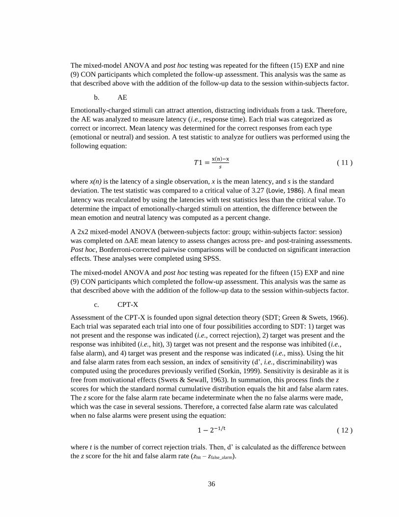
36
The mixed-model ANOVA and post hoc testing was repeated for the fifteen (15) EXP and nine
(9) CON participants which completed the follow-up assessment. This analysis was the same as
that described above with the addition of the follow-up data to the session within-subjects factor.
b. AE
Emotionally-charged stimuli can attract attention, distracting individuals from a task. Therefore,
the AE was analyzed to measure latency (i.e., response time). Each trial was categorized as
correct or incorrect. Mean latency was determined for the correct responses from each type
(emotional or neutral) and session. A test statistic to analyze for outliers was performed using the
following equation:
𝑇1 =x(n)−x
𝑠 ( 11 )
where x(n) is the latency of a single observation, x is the mean latency, and s is the standard
deviation. The test statistic was compared to a critical value of 3.27 (Lovie, 1986). A final mean
latency was recalculated by using the latencies with test statistics less than the critical value. To
determine the impact of emotionally-charged stimuli on attention, the difference between the
mean emotion and neutral latency was computed as a percent change.
A 2x2 mixed-model ANOVA (between-subjects factor: group; within-subjects factor: session)
was completed on ΔAE mean latency to assess changes across pre- and post-training assessments.
Post hoc, Bonferroni-corrected pairwise comparisons will be conducted on significant interaction
effects. These analyses were completed using SPSS.
The mixed-model ANOVA and post hoc testing was repeated for the fifteen (15) EXP and nine
(9) CON participants which completed the follow-up assessment. This analysis was the same as
that described above with the addition of the follow-up data to the session within-subjects factor.
c. CPT-X
Assessment of the CPT-X is founded upon signal detection theory (SDT; Green & Swets, 1966).
Each trial was separated each trial into one of four possibilities according to SDT: 1) target was
not present and the response was indicated (i.e., correct rejection), 2) target was present and the
response was inhibited (i.e., hit), 3) target was not present and the response was inhibited (i.e.,
false alarm), and 4) target was present and the response was indicated (i.e., miss). Using the hit
and false alarm rates from each session, an index of sensitivity (d’, i.e., discriminability) was
computed using the procedures previously verified (Sorkin, 1999). Sensitivity is desirable as it is
free from motivational effects (Swets & Sewall, 1963). In summation, this process finds the z
scores for which the standard normal cumulative distribution equals the hit and false alarm rates.
The z score for the false alarm rate became indeterminate when the no false alarms were made,
which was the case in several sessions. Therefore, a corrected false alarm rate was calculated
when no false alarms were present using the equation:
1 − 2−1/t ( 12 )
where t is the number of correct rejection trials. Then, d’ is calculated as the difference between
the z score for the hit and false alarm rate (zhit – zfalse_alarm).

37
A 2x2 mixed-model ANOVA (between-subjects factor: group; within-subjects factor: session)
was completed on CPT-X d’ to assess changes across pre- and post-training assessments. Post
hoc, Bonferroni-corrected pairwise comparisons will be conducted on significant interaction
effects. These analyses were completed using SPSS.
The mixed-model ANOVA and post hoc testing was repeated for the fifteen (15) EXP and nine
(9) CON participants which completed the follow-up assessment. This analysis was the same as
that described above with the addition of the follow-up data to the session within-subjects factor.
3. Neural Measures
a. A1 Response to Auditory Stimulation
The BOLD data acquired from each functional localizer was processed using FSL. First,
individual (first-level) analyses will be conducted on each of the 4D fMRI data sets. Prior to the
individual analyses, the data sets will be pre-processed in the same manner as that described in
Section III.C.1 above except for the high-pass filter had a cutoff of 40 s. After pre-processing, a
single EV will be defined by convolving a boxcar model containing 20 s rest and task conditions
with a HRF (modeled by a gamma function; phase offset = 0 s, standard deviation = 3 s, mean lag
= 6 s). The temporal derivative of the original waveform will be added to the result, accounting
for small shifts in phase potentially improving the model fit. The temporal filter described above
will be applied to the model, mimicking the pre-processing conducted on the measured data. The
data set will be fit to the model using a GLM with prewhitening by applying a weight of +1 to the
EV. This will be representative of activation during the task (positive correlation with the model).
Z statistic maps will be created using standard statistical transforms to convert the β parameter
maps. A clustering method will allow us to account for false positives due to multiple
comparisons. This method considers adjacent voxels with a z statistic of 2.3 or greater to be a
cluster. The significance of each cluster will be estimated and compared to a threshold of p < 0.05
using Gaussian Random Field theory. Voxels that either do not pass the significance level
threshold or do not belong to a cluster will be set to zero. A mean image of the data set will be
registered to the individual’s high-resolution structural image by estimating motion from a
boundary-based registration method including a fieldmap-based distortion correction (Greve &
Fischl, 2009), then will be further registered to the MNI-152 T1-weighted 2 mm template
provided in FSL using a 12-parameter model. The z statistic maps will be converted to standard
space using the transform responsible for morphing the mean image of each data set to the
template to co-register all volumes.
ROIs for the left and right A1 will be created from the Talairach atlas (Talairach & Tournoux,
1988). Indices for each region will be extracted and transformed to the Montreal Neurological
Institute (MNI) space using the Talairach-to-ICBM transform (Lancaster et al., 2007). Resulting
MNI coordinates will be will be translated into image indices (including rounding to the next
highest integer). Binary masks representing each ROI will be created by setting the value of each
index to 1 and all others to 0. Average activation in each ROI will be computed from the voxels
which survived the cluster-based correction for multiple comparisons and whose value are above
a threshold of Z = 2.3. A 2x2x2 (between-subjects factor: group, within-subjects factors: session
and hemisphere) mixed-model ANOVA will be conducted on the left and right A1 average
activity using SPSS. A significant session by group or session by group and hemisphere
interaction will indicate differential changes in A1 activity across groups and training, supportive

38
of Hypothesis 3. Post hoc, pairwise, Bonferroni-corrected comparisons will be conducted in SPSS
to compare A1 activity between groups at session 1 and 5 separately. We anticipate similar
activity across groups at session 1, while a significant difference at session 5, with the
experimental group showing reduced activity which will further support Hypothesis 3.
b. Resting-State Activity
The BOLD data acquired from the pre- and post-training resting-state fMRI was processed using
FSL. Prior to the analysis, the data sets were pre-processed in the same manner as that described
in Section III.C.1 except for the high-pass filter had a cutoff of 30 s. ICA was conducted on the
pre-processed data. The MELODIC software of FSL will conduct a probabilistic ICA (Beckmann
& Smith, 2004) using multisession temporal concatenation to create standard-order IC maps (the
number of ICs will be approximately 1/4 to 1/6 of the total volumes acquired). Resulting IC maps
were thresholded using an alternative hypothesis based on the fit of a Gaussian/gamma mixture
model to the distribution of voxel intensities within the spatial maps (Beckmann, DeLuca, Devlin,
& Smith, 2005) and a p < 0.05.
In a group analysis, voxel-based comparisons were made between groups and sessions using a
dual-regression technique (Filippini et al., 2009; Littow et al., 2010; Veer et al., 2010). This
technique performs multiple linear regression of the z statistic group IC maps against the
individual pre-processed BOLD data to produce subject-variance normalized time courses for
each component. Multiple linear regression of these time courses was then carried out against the
pre-processed individual data sets to create subject-specific spatial maps. Non-parametric
statistical differences were determined using permutation testing implemented using FSL
Randomize incorporating threshold-free cluster enhancement (TFCE; Smith & Nichols, 2009).
Null t distributions for a contrasts representative of the main effect of session and the interaction
of session by group were derived by performing 1000 random permutations (Nichols & Holmes,
2002). Resultant z statistic difference maps were thresholded at p < 0.05 (corrected for family-
wise error using TFCE) and resampled into standard space. The difference maps from the
component representing the auditory network10 were assessed. In the resulting 1-p images, voxels
identified in the interaction effect of session by group at session 5 will indicate regions of the
auditory network responding to fMRI-NFT11, supportive of Hypothesis 4.
In an exploratory analysis, the IC maps from the components representing the default mode and
executive control networks12 were assessed in the same manner described above. In the resulting
1-p images, voxels identified in the effect of group at session 5 will indicate network nodes
responding to fMRI-NFT.
10 The component representing this network was determined from visual inspection of all the IC maps
generated from the group multisession temporal concatenation ICA processing.
11 In the 1-p images, voxels with a value between 0.95 and 1.0 (one-tailed) will indicate significant results
when assessing only a single component.
12 The components representing these networks will be determined from visual inspection of all the IC
maps generated from the group multisession temporal concatenation ICA processing.

39
c. Steady-State Perfusion
Steady-state perfusion was assessed from ASL to quantify CBF. CBF was measured in units of
mL/100 mg/min. Data was extracted from ROIs encompassing the left and right A1, ACC, medial
frontal gyrus (MeFG), and STG using the Talairach atlas (Talairach & Tournoux, 1988). ROIs
were generated in the same manner as described in Section Error! Reference source not found..
The proton density-weighted images acquired were registered to the individual’s high-resolution
structural image by estimating motion from a boundary-based registration method including a
fieldmap-based distortion correction (Greve & Fischl, 2009), then further registered to the MNI-
152 T1-weighted 2 mm template provided in FSL (Collins et al., 1995; Mazziotta et al., 2001)
using a 12-parameter model (Jenkinson & Smith, 2001; Jenkinson et al., 2002). The CBF maps
were converted to standard space using the transform responsible for morphing the proton
density-weighted image of each data set to the template in order to co-register all volumes. Data
from two (2) participants (1 CON, 1 EXP) was corrupted, therefore the analysis includes the
remaining 8 CON and 17 EXP participants. 2x2x2 (between-subjects factor: group; within-
subjects factors: session and hemisphere) mixed-model ANOVAs were carried out for each ROI.
A significant session by group interaction, with the experimental group showing a greater
reduction in perfusion will provide evidence for Hypothesis 5.
Results
A. A1 Control
A mixed-model ANOVA evaluated the effects of group, session, and run on A1 activity during
closed-loop neuromodulation. A1 activity is representative of an individual’s ability to self-
regulate brain activity of A1 (i.e., A1 control). The descriptive statistics for this data is presented
in Table 3. The results of the tests of between-subjects effects (Table 4) revealed a significant
main effect of group (p = 0.029, one-tailed). One-tailed statistics are reported as the a priori
hypothesis that A1 control would be greater in the EXP group. The ANOVA analysis included
Mauchly’s Test of Sphericity (Table 5) which determined that the variances of the differences
between all possible pairs of within-subject conditions were not significant for the main effect of
session (p = 0.160, two-tailed) or the interaction of session and run (p = 0.776, two-tailed). This
test could not be conducted on the main effect of run because there is only a single difference to
compute and, therefore, no comparison to be made. These results validate the assumption of
sphericity, which will be used to assess the results of the within-subjects tests henceforth. The
results of the within-subjects testing (Table 6) identify a significant main effect of session (Figure
15; p = 0.0175, one-tailed). One-tailed statistics are reported as our a priori hypothesis that A1
control would increase with training. The main effect of run was not significant (p > 0.05). The
interaction effects of session by group, run by group, session by run, and session by group and
run are not significant (p > 0.05).

40
Table 3. Descriptive statistics for A1 control measures separated by factors session, run, and
group.
Session Run Group
Mean A1 Control
(z statistic) Std. Deviation N
1
1
CON -.513575 1.8176834 9
EXP -.109704 1.5335134 18
Total -.244328 1.6099299 27
2
CON -.364050 1.0258848 9
EXP 1.009057 2.0692044 18
Total .551354 1.8863820 27
2
1
CON .328114 2.5873677 9
EXP 1.842709 2.7490086 18
Total 1.337844 2.7441516 27
2
CON -.079995 2.7550314 9
EXP 2.047707 2.1369636 18
Total 1.338473 2.5230988 27
3
1
CON .967520 3.1121580 9
EXP 1.605297 2.7123791 18
Total 1.392705 2.8079132 27
2
CON .203470 2.1023534 9
EXP 1.971905 3.1324199 18
Total 1.382427 2.9150025 27
4
1
CON .587748 2.6300614 9
EXP 1.979438 2.5839438 18
Total 1.515541 2.6345602 27
2
CON .431830 2.2720221 9
EXP 1.658697 2.8785080 18
Total 1.249741 2.7117029 27
5
1
CON .391666 2.6307519 9
EXP 3.201307 3.0964049 18
Total 2.264760 3.1968894 27
2
CON -.075156 2.5194464 9
EXP 2.229866 3.4949272 18
Total 1.461525 3.3415013 27
Table 4. Results of the between-subjects tests from the mixed-model ANOVA. Power is
computed using an alpha of 0.05.
Source
Type III Sum
of Squares df
Mean
Square F
Sig.
(one-tailed)
Partial Eta
Squared
Observed
Power
Intercept 22.381 1 22.381 6.073 .011 .195 .659
Group 14.524 1 14.524 3.941 .029 .136 .480
Error 92.135 25 3.685
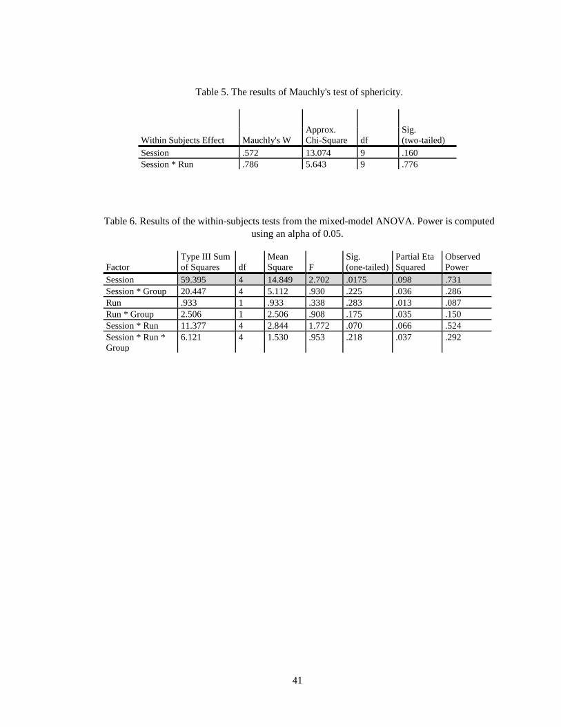
41
Table 5. The results of Mauchly's test of sphericity.
Within Subjects Effect Mauchly's W
Approx.
Chi-Square df
Sig.
(two-tailed)
Session .572 13.074 9 .160
Session * Run .786 5.643 9 .776
Table 6. Results of the within-subjects tests from the mixed-model ANOVA. Power is computed
using an alpha of 0.05.
Factor
Type III Sum
of Squares df
Mean
Square F
Sig.
(one-tailed)
Partial Eta
Squared
Observed
Power
Session 59.395 4 14.849 2.702 .0175 .098 .731
Session * Group 20.447 4 5.112 .930 .225 .036 .286
Run .933 1 .933 .338 .283 .013 .087
Run * Group 2.506 1 2.506 .908 .175 .035 .150
Session * Run 11.377 4 2.844 1.772 .070 .066 .524
Session * Run *
Group
6.121 4 1.530 .953 .218 .037 .292

42
Figure 15. A1 Control averaged across groups and runs for each session. The main effect of
session was found to be significant (p = 0.0175, one-tailed, sphericity assumed).
Post hoc Bonferroni-corrected pairwise comparisons were conducted on the session by group
interaction (Table 7). These results revealed no significant difference between session 1 and 5 for
the CON group (p > 0.05) however a significant difference between these sessions were identified
in the EXP group (p = 0.0165, one-tailed). Furthermore, there was a significant difference
between sessions 1 and 2 for the EXP group (p = 0.038, one-tailed).

43
Figure 16. A1 control averaged across runs separated by group and session. The post hoc
pairwise comparisons did not reveal any significant differences for the CON group, however
sessions 2 (p = 0.038, one-tailed, Bonferroni-corrected) and 5 (p = 0.0165, one-tailed, Bonferroni-
corrected) were found to be significantly greater than session 1 for the EXP group.

44
Table 7. Results of the post hoc pairwise comparisons for the session interaction with group.
Confidence intervals and statistical significance was computed using Bonferroni correction for
multiple comparisons. Statistical significance reported is one-tailed due to the a priori
hypotheses.
Group
(I)
Session
(J)
Session
Mean
Difference (I-J) Std. Error Sig.
95% Confidence Interval for
Difference
Lower Bound Upper Bound
CON
1
2 -.563 .730 1.000 -2.808 1.683
3 -1.024 .802 1.000 -3.494 1.446
4 -.949 .813 1.000 -3.451 1.554
5 -.597 .978 1.000 -3.607 2.413
2
3 -.461 .719 1.000 -2.676 1.753
4 -.386 .828 1.000 -2.935 2.163
5 -.034 .829 1.000 -2.586 2.518
3 4 .076 .742 1.000 -2.208 2.360
5 .427 .739 1.000 -1.848 2.702
4 5 .352 .571 1.000 -1.407 2.110
EXP
1
2 -1.496 .516 .038 -3.083 .092
3 -1.339 .567 .132 -3.086 .408
4 -1.369 .575 .125 -3.139 .400
5 -2.266 .692 .0165 -4.395 -.137
2
3 .157 .509 1.000 -1.409 1.722
4 .126 .586 1.000 -1.676 1.928
5 -.770 .586 1.000 -2.575 1.034
3 4 -.030 .525 1.000 -1.646 1.585
5 -.927 .523 .441 -2.535 .682
4 5 -.897 .404 .178 -2.140 .347
B. Behavior
1. ACS
Mixed-model ANOVAs evaluated the effects of group and session on ACS total score. The ACS
total score is a subjective measure of attentional control. First are presented the results of the
ANOVA which evaluated the ACS scores for sessions 1 and 5 (Table 8). The results of the tests
of between-subjects effects revealed main effect of group was not significant (Table 9; p > 0.05,
one-tailed). One-tailed statistics are reported as the a priori hypothesis that ACS total score
would be greater in the EXP group. Mauchly’s Test of Sphericity could not be conducted on the
within-subjects factors because there is only a single difference to compute and, therefore, no
comparison to be made. However, this test was conducted and significant on the 2x3 ANOVA
(analysis and results below), therefore the assumption of sphericity is not validated and
Greenhouse-Geisser correction will be applied. The results of the within-subjects testing (Table
10) identified the main effect of session was not significant (Figure 17; p > 0.05, one-tailed).
One-tailed statistics are reported as our a priori hypothesis that ACS total score would increase
with training. The interaction effect of session and group was not significant (p > 0.05), therefore
no post hoc testing was performed.

45
Table 8. Descriptive statistics for ACS total score for sessions 1 and 5 separated by group.
Session Group Mean ACS total score Std. Deviation N
1
CON 49.3333 8.70345 9
EXP 49.6667 9.39336 18
Total 49.5556 9.00142 27
5
CON 48.8889 8.63777 9
EXP 49.8889 11.51924 18
Total 49.5556 10.48564 27
Table 9. Results of the between-subjects tests from the 2x2 mixed-model ANOVA. Power is
computed using an alpha of 0.05.
Source
Type III Sum
of Squares df
Mean
Square F
Sig.
(one-tailed)
Partial Eta
Squared
Observed
Power
Intercept 58674.074 1 58674.074 632.536 < .001 .962 1.000
Group 2.667 1 2.667 .029 .433 .001 .053
Error 2319.000 25 92.760
Table 10. Results of the within-subjects tests from the 2x2 mixed-model ANOVA. Power is
computed using an alpha of 0.05.
Factor
Type III Sum
of Squares df
Mean
Square F
Sig.
(one-tailed)
Partial Eta
Squared
Observed
Power
Session .148 1 .148 .012 .457 .000 .051
Session * Group 1.333 1 1.333 .104 .375 .004 .061

46
Figure 17. ACS total score averaged across participants for each group and session. No
significant main effects or interactions were found.
Next are the results from the 2x3 mixed-model ANOVA which evaluated the ACS scores for
sessions 1, 5, and the follow-up (Table 11). The results of the tests of between-subjects effects
revealed main effect of group was not significant (Table 12; p > 0.05, one-tailed). One-tailed
statistics are reported as the a priori hypothesis that ACS total score would be greater in the EXP
group. Mauchly’s Test of Sphericity was significant (Table 13; p = 0.02, two-tailed), therefore the
assumption of sphericity is not validated and Greenhouse-Geisser correction will be applied. The
results of the within-subjects testing (Table 14) identified the main effect of session was not
significant (Figure 18; p > 0.05, one-tailed). One-tailed statistics are reported as our a priori
hypothesis that ACS total score would increase with training. The interaction effect of session
and group was not significant (p > 0.05), therefore no post hoc testing was performed.

47
Table 11. Descriptive statistics for ACS total score for sessions 1, 5, and the follow-up separated
group.
Session Group Mean ACS total score Std. Deviation N
1
CON 49.3333 8.70345 9
EXP 49.5333 9.73115 15
Total 49.4583 9.16505 24
5
CON 48.8889 8.63777 9
EXP 50.2000 12.07832 15
Total 49.7083 10.73183 24
Follow-Up
CON 49.3333 11.55422 9
EXP 49.8667 12.64836 15
Total 49.6667 11.99517 24
Table 12. Results of the between-subjects tests from the 2x3 mixed-model ANOVA. Power is
computed using an alpha of 0.05.
Source
Type III Sum
of Squares df
Mean
Square F
Sig.
(one-tailed)
Partial Eta
Squared
Observed
Power
Intercept 55188.390 1 55188.390 516.320 < .001 .959 1.000
Group 2.612 1 2.612 .024 .438 .001 .053
Error 2351.536 22 106.888
Table 13. The results of Mauchly's test of sphericity.
Within-Subjects Effect Mauchly's W
Approx.
Chi-Square df
Sig.
(two-tailed)
Session .689 7.836 2 .020
Table 14. Results of the within-subjects tests from the 2x3 mixed-model ANOVA. Power is
computed using an alpha of 0.05.
Factor
Type III Sum
of Squares df
Mean
Square F
Sig.
(one-tailed)
Partial Eta
Squared
Observed
Power
Session .324 1.525 .212 .009 .488 .000 .051
Session * Group 3.657 1.525 2.398 .098 .428 .004 .062

48
Figure 18. ACS total score averaged across participants for each group and session. No
significant main effects or interactions were found.
2. AE
Mixed-model ANOVAs evaluated the effects of group and session on ΔAE mean latency. First
are the results of the ANOVA which evaluated sessions 1 and 5 (Table 15). The results of the
tests of between-subjects effects (Table 16) revealed the main effect of group was significant (p =
0.042, one-tailed), with a larger impact of emotionally-charged stimuli on attention in the EXP
group. Mauchly’s Test of Sphericity could not be conducted on the within-subjects factors
because there is only a single difference to compute and, therefore, no comparison to be made.
However, this test was conducted on the 2x3 ANOVA (analysis and results below) but was not
significant for the main effect of session (p > 0.05). Therefore, the assumption of sphericity is
valid. The results of the within-subjects testing (Table 17) identified the main effect of session
and the session by group interaction effect were not significant (Figure 19; p > 0.05). One-tailed
statistics are reported as our a priori hypothesis that the impact of emotionally-charged stimuli
would decrease with training.

49
Table 15. Descriptive statistics for ΔAE mean latency for sessions 1 and 5 separated by group
and emotion.
Session Group ΔAE Mean Latency (%) Std. Deviation (ms) N
1
CON .3178 5.07895 9
EXP 3.5611 6.42796 18
Total 2.4800 6.11397 27
5
CON 1.0833 6.68607 9
EXP 3.9639 4.94246 18
Total 3.0037 5.62511 27
Table 16. Results of the between-subjects tests from the 2x2 mixed-model ANOVA. Power is
computed using an alpha of 0.05.
Source
Type III Sum of
Squares df Mean Square F
Sig.
(one-tailed)
Partial Eta
Squared
Observed
Power
Intercept 119.513 1 119.513 6.940 .007 .217 .716
Group 56.253 1 56.253 3.267 .042 .116 .412
Error 430.527 25 17.221
Table 17. Results of the within-subjects tests from the 2x2 mixed-model ANOVA. Power is
computed using an alpha of 0.05.
Factor
Type III Sum
of Squares df
Mean
Square F
Sig.
(one-tailed)
Partial Eta
Squared
Observed
Power
Session 4.095 1 4.095 .125 .364 .005 .063
Session * Group .395 1 .395 .012 .457 .000 .051

50
Figure 19. ΔAE mean latency averaged across participants for each session and group. ΔAE
mean latency was found to be significantly greater in the EXP group.
Next are the results from the 2x3 mixed-model ANOVA which evaluated the ΔAE mean latency
for sessions 1, 5, and the follow-up (Table 18). The results of the tests of between-subjects effects
(Table 19) revealed the main effect of group was not significant (p > 0.05, one-tailed). One-tailed
statistics are reported as the a priori hypothesis that AE latency would be lower in the EXP
group. Mauchly’s Test of Sphericity was not significant for the main effect of session (Table 21;
p > 0.05, two-tailed), therefore the assumption of sphericity was validated. The results of the
within-subjects testing (Table 21) identified the main effect of session and the session by group
interaction were not significant (Figure 20; p > 0.05, one-tailed). One-tailed statistics are reported
as our a priori hypothesis that the impact of emotionally-charged stimuli would decrease with
training.

51
Table 18. Descriptive statistics for ΔAE mean latency for sessions 1, 5, and the follow-up
separated by group and emotion.
Session Group ΔAE Mean Latency (%) Std. Deviation (ms) N
1
CON .3178 5.07895 9
EXP 2.9673 6.57527 15
Total 1.9738 6.08323 24
5
CON 1.0833 6.68607 9
EXP 3.9313 5.32265 15
Total 2.8633 5.89724 24
Follow-Up
CON 2.9371 4.57266 9
EXP 1.1399 5.81798 15
Total 1.8138 5.35410 24
Table 19. Results of the between-subjects tests from the 2x3 ANOVA. Power is computed using
an alpha of 0.05.
Source
Type III Sum of
Squares df Mean Square F
Sig.
(one-tailed)
Partial Eta
Squared
Observed
Power
Intercept 95.740 1 95.740 7.626 .006 .257 .752
Group 8.558 1 8.558 .682 .209 .030 .124
Error 276.182 22 12.554
Table 20. The results of Mauchly's test of sphericity for the 2x3 ANOVA.
Within-Subjects Effect Mauchly's W
Approx.
Chi-Square df
Sig.
(two-tailed)
Session .911 1.964 2 .375
Table 21. Results of the within-subjects tests from the 2x3 ANOVA. Power is computed using
an alpha of 0.05.
Factor
Type III Sum
of Squares df
Mean
Square F
Sig.
(one-tailed)
Partial Eta
Squared
Observed
Power
Session 8.433 2 4.217 .135 .437 .006 .069
Session * Group 77.609 2 38.804 1.239 .150 .053 .256
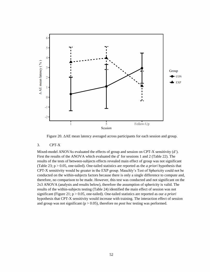
52
Figure 20. ΔAE mean latency averaged across participants for each session and group.
3. CPT-X
Mixed-model ANOVAs evaluated the effects of group and session on CPT-X sensitivity (d’).
First the results of the ANOVA which evaluated the d’ for sessions 1 and 2 (Table 22). The
results of the tests of between-subjects effects revealed main effect of group was not significant
(Table 23; p > 0.05, one-tailed). One-tailed statistics are reported as the a priori hypothesis that
CPT-X sensitivity would be greater in the EXP group. Mauchly’s Test of Sphericity could not be
conducted on the within-subjects factors because there is only a single difference to compute and,
therefore, no comparison to be made. However, this test was conducted and not significant on the
2x3 ANOVA (analysis and results below), therefore the assumption of sphericity is valid. The
results of the within-subjects testing (Table 24) identified the main effect of session was not
significant (Figure 21; p > 0.05, one-tailed). One-tailed statistics are reported as our a priori
hypothesis that CPT-X sensitivity would increase with training. The interaction effect of session
and group was not significant (p > 0.05), therefore no post hoc testing was performed.

53
Table 22. Descriptive statistics for CPT-X d’ for sessions 1 and 5 separated by group.
Session Group Mean CPT-X d’ Std. Deviation N
1
CON 3.5175 .44068 9
EXP 3.4090 .37979 18
Total 3.4452 .39596 27
5
CON 3.6271 .57090 9
EXP 3.4995 .50729 18
Total 3.5420 .52183 27
Table 23. Results of the between-subjects tests from the 2x2 mixed-model ANOVA. Power is
computed using an alpha of 0.05.
Source
Type III Sum
of Squares df
Mean
Square F
Sig.
(one-tailed)
Partial Eta
Squared
Observed
Power
Intercept 296.233 1 296.233 1795.844 < .001 .986 1.000
Group .084 1 .084 .507 .242 .020 .105
Error 4.124 25 .165
Table 24. Results of the within-subjects tests from the 2x2 mixed-model ANOVA. Power is
computed using an alpha of 0.05.
Factor
Type III Sum
of Squares df
Mean
Square F
Sig.
(one-tailed)
Partial Eta
Squared
Observed
Power
Session .120 1 .120 1.095 .153 .042 .172
Session * Group .001 1 .001 .010 .461 .000 .051
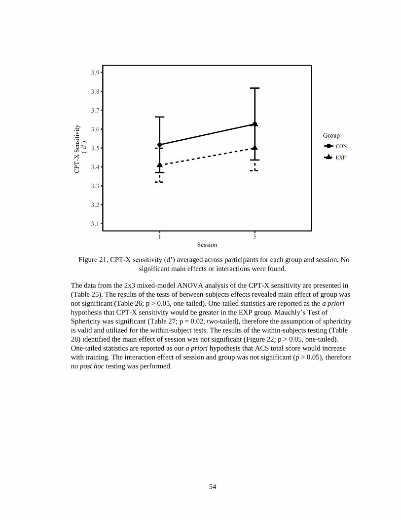
54
Figure 21. CPT-X sensitivity (d’) averaged across participants for each group and session. No
significant main effects or interactions were found.
The data from the 2x3 mixed-model ANOVA analysis of the CPT-X sensitivity are presented in
(Table 25). The results of the tests of between-subjects effects revealed main effect of group was
not significant (Table 26; p > 0.05, one-tailed). One-tailed statistics are reported as the a priori
hypothesis that CPT-X sensitivity would be greater in the EXP group. Mauchly’s Test of
Sphericity was significant (Table 27; p = 0.02, two-tailed), therefore the assumption of sphericity
is valid and utilized for the within-subject tests. The results of the within-subjects testing (Table
28) identified the main effect of session was not significant (Figure 22; p > 0.05, one-tailed).
One-tailed statistics are reported as our a priori hypothesis that ACS total score would increase
with training. The interaction effect of session and group was not significant (p > 0.05), therefore
no post hoc testing was performed.

55
Table 25. Descriptive statistics for CPT-X sensitivity for sessions 1, 5, and the follow-up
separated group.
Session Group Mean CPT-X d’ Std. Deviation N
1
CON 3.5175 .44068 9
EXP 3.3937 .40907 15
Total 3.4402 .41612 24
5
CON 3.6271 .57090 9
EXP 3.4806 .47020 15
Total 3.5356 .50318 24
Follow-Up
CON 3.4909 .47909 9
EXP 3.3489 .63650 15
Total 3.4022 .57565 24
Table 26. Results of the between-subjects tests from the 2x3 mixed-model ANOVA. Power is
computed using an alpha of 0.05.
Source
Type III Sum
of Squares df
Mean
Square F
Sig.
(one-tailed)
Partial Eta
Squared
Observed
Power
Intercept 271.931 1 271.931 1375.944 < .001 .984 1.000
Group .106 1 .106 .538 .236 .024 .108
Error 4.348 22 .198
Table 27. The results of Mauchly's test of sphericity.
Within-Subjects Effect Mauchly's W
Approx.
Chi-Square df
Sig.
(two-tailed)
Session .794 4.836 2 .089
Table 28. Results of the within-subjects tests from the 2x3 mixed-model ANOVA. Power is
computed using an alpha of 0.05.
Factor
Type III Sum
of Squares df
Mean
Square F
Sig.
(one-tailed)
Partial Eta
Squared
Observed
Power
Session .217 2 .108 1.172 .159 .051 .244
Session * Group .002 2 .001 .009 .496 .000 .051

56
Figure 22. CPT-X sensitivity averaged across participants for each group and session. No
significant main effects or interactions were found.
C. Neural Measures
1. A1 Response to Auditory Stimulation
A mixed-model ANOVA evaluated the effects of group, session, and hemisphere on A1 activity
during continuous noise stimulation. The results of the test of between-subjects effects revealed
the main effect of group was not significant (Table 29; p > 0.05, one-tailed). One-tailed statistics
are reported as the a priori hypothesis that A1 activity would be lower in the EXP group.
Mauchly’s Test of Sphericity could not be conducted on the within-subjects factors because there
is only a single difference to compute and, therefore, no comparison to be made and sphericity
was assumed. The results of the within-subjects testing (Table 30) identified the main effect of
session was significant (p = 0.0115, one-tailed), with decreased activation in session 5 (Figure
23). One-tailed statistics are reported as our a priori hypothesis that A1 activity induced from
continuous noise stimulation would decrease with training. All other main effects and interactions
were not significant (p > 0.05), therefore no post hoc testing was performed.

57
Table 29. Results of the between-subjects tests from the 2x2x2 mixed-model ANOVA for A1
activity during continuous noise stimulation. Power is computed using an alpha of 0.05.
Source
Type III Sum
of Squares df
Mean
Square F
Sig.
(one-tailed)
Partial Eta
Squared
Observed
Power
Intercept 60.390 1 60.390 60.158 .000 .706 1.000
Group .003 1 .003 .003 .478 .000 .050
Error 25.096 25 1.004
Table 30. Results of the within-subjects tests from the 2x2 mixed-model ANOVA. Power is
computed using an alpha of 0.05.
Factor
Type III Sum
of Squares df
Mean
Square F
Sig.
(one-tailed)
Partial Eta
Squared
Observed
Power
Session 14.184 1 14.184 5.844 0.0115 .189 .642
Session * Group 2.907 1 2.907 1.198 0.142 .046 .183
Hemisphere .550 1 .550 .612 0.2205 .024 .117
Hemisphere * Group .899 1 .899 .999 0.1635 .038 .161
Session * Hemisphere .626 1 .626 1.774 0.0975 .066 .249
Session * Hemisphere
* Group .223 1 .223 .632 0.217 .025 .119
Figure 23. A1 activity in response to continuous noise stimulation. Averaged across groups and
hemispheres, activity during session 5 was significantly lower than session 1.

58
2. Resting-State Activity
Probabilistic ICA resulted in 63 components identified automatically, approximately 1/5 of the
total volumes acquired). From these components, three (3) components were identified each
representing the auditory network (Figure 24), DMN (Figure 25), or the executive control
network (Figure 26).
Figure 24. Resting auditory network. Axial slices are displayed at MNI coordinates z = 2, 10 and
20 mm (left to right). Coronal slices are displayed at MNI coordinates y = 0, 26, and 34 mm (left
to right).

59
Figure 25. Default mode network. Axial slices are displayed at MNI coordinates z = 18, 22, and
42 mm (left to right). Coronal slices are displayed at MNI coordinates y = 32, 48, and 52 mm (left
to right).

60
Figure 26. Resting executive control network. Axial slices are displayed at MNI coordinates z =
0, 4, and 6 mm (left to right). Coronal slices are displayed at MNI coordinates y = 32, 42, and 52
mm (left to right).
A voxel-wise dual-regression technique was carried out to assess the effect of session and session
by group on these three networks. There was no main effect of session within the executive
control network (p > 0.05), however there was a significant main effect of session in the auditory
network and DMN (p < 0.05, one-tailed). Regions in the auditory network were found to have
significantly enhanced connectivity over the course of training were identified as the left STG,
transverse temporal gyrus, and postcentral gyrus (Figure 27). For the DMN, enhanced
connectivity (Figure 28) over training were found predominately in the left hemisphere: BA19,
precuneus, middle frontal gyrus, supramarginal gyrus, and the inferior parietal lobule; but
bilateral effects were observed in the superior frontal gyrus. Additionally, increased connectivity
was observed in the right transverse temporal gyrus. No significant session by group interaction
was found in any of the three networks (p > 0.05, one-tailed).
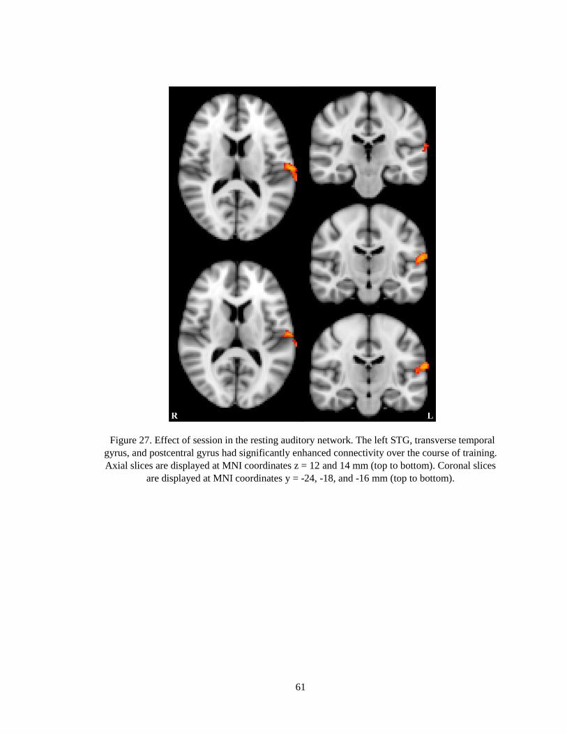
61
Figure 27. Effect of session in the resting auditory network. The left STG, transverse temporal
gyrus, and postcentral gyrus had significantly enhanced connectivity over the course of training.
Axial slices are displayed at MNI coordinates z = 12 and 14 mm (top to bottom). Coronal slices
are displayed at MNI coordinates y = -24, -18, and -16 mm (top to bottom).

62
Figure 28. Effect of session in the DMN. Enhanced connectivity was observed only in the left
hemisphere include BA19, precuneus, middle frontal gyrus, supramarginal gyrus, and the inferior
parietal lobule; while the right transverse temporal gyrus demonstrated increased connectivity.
Bilateral increased connectivity was observed in the superior frontal gyrus. Axial slices are
displayed at MNI coordinates z = 10, 30, 34, 38, and 58 mm (left to right). Coronal slices are
displayed at MNI coordinates y = -56, -40, -18, 22, and 24 mm (top to bottom).
3. Steady-State Perfusion
Mixed-model ANOVAs evaluated the effects of group, session, and hemisphere on CBF from
four ROIs (Appendix I). The results of the tests of between-subjects effects revealed main effect
of group was not significant for all four ROIs (Table 31; p > 0.05, one-tailed). One-tailed
statistics are reported as the a priori hypothesis that resting CBF would be lower in the EXP
group. Mauchly’s Test of Sphericity could not be conducted on the within-subjects factors
because there is only a single difference to compute and, therefore, no comparison to be made and
sphericity was assumed. The results of the within-subjects testing identified the main effect of
hemisphere was significant for all four ROIs (Table 32; p < 0.05, one-tailed). One-tailed statistics
are reported as our a priori hypothesis that resting CBF would decrease with training.
Interestingly, the right hemisphere had greater resting CBF than the left for regions associated
with auditory processing (A1 and STG) while the opposite was found for regions involved in
attentional processes (ACC, MeFG). All other main effects and interactions were not significant
(p > 0.05), therefore no post hoc testing was performed.

63
Table 31. Results of the between-subjects tests from the 2x2x2 mixed-model ANOVAs for each
ROI. Power is computed using an alpha of 0.05.
ROI Source
Type III Sum
of Squares df
Mean
Square F
Sig.
(one-tailed)
Partial Eta
Squared
Observed
Power
A1
Intercept 80669.702 1 80669.7 1294.546 < .001 .983 1.000
Group 60.661 1 60.661 .973 .167 .041 0.157
Error 1433.246 23 62.315
STG
Intercept 67839.499 1 67839.4 1487.024 < .001 .985 1.000
Group 42.684 1 42.684 .936 .172 .039 .153
Error 1049.282 23 45.621
ACC
Intercept 48951.536 1 48951.5 1376.936 < .001 .984 1.000
Group 40.794 1 40.794 1.147 .148 .048 .177
Error 817.675 23 35.551
MeFG
Intercept 57576.836 1 57576.8 1250.924 < .001 .982 1.000
Group 10.228 1 10.228 .222 .321 .010 .074
Error 1058.632 23 46.027

64
Table 32. Results of the within-subjects tests from the 2x2x2 mixed-model ANOVAs for each
ROI. Power is computed using an alpha of 0.05.
ROI Factor
Type III Sum
of Squares df
Mean
Square F
Sig.
(one-tailed)
Partial Eta
Squared
Observed
Power
A1
Session 6.498 1 6.498 .169 .3425 .007 .068
Session * Group 3.845 1 3.845 .100 .3775 .004 .061
Hemisphere 457.388 1 457.388 31.631 < .001 .579 1.000
Hemisphere *
Group .031 1 .031 .002 .4815 .000 .050
Session *
Hemisphere 7.253E-5 1
7.253E-
5 .000 .4985 .000 .050
Session *
Hemisphere *
Group
.002 1 .002 .000 .493 .000 .050
STG
Session 1.540 1 1.540 .052 .411 .002 .055
Session * Group 11.472 1 11.472 .386 .27 .017 .092
Hemisphere 270.734 1 270.734 34.566 < .001 .600 1.000
Hemisphere *
Group .085 1 .085 .011 .459 .000 .051
Session *
Hemisphere 2.160 1 2.160 .732 .2005 .031 .130
Session *
Hemisphere *
Group
7.530 1 7.530 2.551 .062 .100 .334
ACC
Session 21.120 1 21.120 .960 .1685 .040 .156
Session * Group 11.858 1 11.858 .539 .235 .023 .108
Hemisphere 3693.343 1 3693.34 224.74 < .001 .907 1.000
Hemisphere *
Group 5.433 1 5.433 .331 .2855 .014 .085
Session *
Hemisphere 3.208 1 3.208 .884 .1785 .037 .147
Session *
Hemisphere *
Group
.965 1 .965 .266 .3055 .011 .078
MeFG
Session 3.449 1 3.449 .118 .367 .005 .063
Session * Group 12.837 1 12.837 .440 .257 .019 .097
Hemisphere 2289.514 1 2289.51 292.96 < .001 .927 1.000
Hemisphere *
Group 10.120 1 10.120 1.295 .1335 .053 .194
Session *
Hemisphere 1.519 1 1.519 .703 .205 .030 .127
Session *
Hemisphere *
Group
1.115 1 1.115 .516 .24 .022 .106
D. Bivariate Correlation
Changes across training in behavior (session 5 minus session 1) and A1 control (session 5, run 2
minus session 1 run 1) were computed. Bivariate correlations (Table 33) were carried out in SPSS
to evaluate the relationship between these changes in behavior and A1 control under the

65
hypothesis that those individuals with the greatest change in A1 control will have more profound
changes in behavior. The change in A1 control was found to have a significant negative
correlation with the change in ΔAE mean latency (Pearson’s r = -0.323, p = 0.05). The change in
ACS total score and CPT-X sensitivity were not significantly correlated to A1 control.
Table 33. Results of the bivariate correlation analysis.
ACS Total Score
CPT-X Sensitivity
(d’)
ΔAE Mean Latency
(%)
A1 control
Pearson’s r .244 .119 -.323
Significance
(one-tailed) .110 .277 .050
n 27 27 27
Figure 29. Bivariate correlation revealed a significant negative relationship between the change
in A1 control and the change in ΔAE mean latency.
Discussion
The ability to induce and/or control neural plasticity holds the promise of enhancing recovery
from brain injury (Johnston et al., 2011; Veit et al., 2012) and combating brain disorders and
diseases (Hamilton, Glover, Hsu, Johnson, & Gotlib, 2011; Vaughan et al., 2006), as well as
improving human performance in healthy subjects (deCharms et al., 2005; Haller et al., 2010;
Logothetis, Pauls, Augath, Trinath, & Oeltermann, 2001; Sherwood, Kane, Weisend, & Parker,
2016). Of the techniques currently being explored, endogenous neuromodulation techniques (Mak

66
& Wolpaw, 2009; Smith et al., 2004; Sulzer et al., 2013) have the advantages of no known side
effects and may be translated to exercises that could be performed at home without the use of
sophisticated equipment and trained professionals (Caria et al., 2007; Linden et al., 2012). Real-
time functional magnetic resonance imaging (Cox, Jesmanowicz, & Hyde, 1995; Weiskopf et al.,
2007) has seen a dramatic rise in interest since its advent in 1995, with a large portion of research
dedicated to its application for training endogenous neuromodulation. In this technique, termed
closed-loop neuromodulation, the fMRI signal is measured from a specific region of the brain,
processed, and presented to the subject in real-time. Through training, subjects develop self-
directed mental processing techniques that regulate this signal.
The study presented in this work trained self-regulation of A1 using fMRI-NFT. The
experimental group attempted self-regulation with the aid of real information regarding the
current BOLD signals in A1 while the control group was supplied sham feedback yoked from a
random participant in the experimental group and matched for training progress. In both groups,
the bilateral A1 was identified both anatomically and functionally using an activation map
produced during binaural continuous noise stimulation at each of the five training sessions. The
results indicate an overall increase in the ability to volitionally decrease A1 activity across
training (Figure 15), a region known to be hyperactive in chronic tinnitus. Furthermore, self-
control over A1 deactivation between the first and last training session was significantly
increased in the experimental group. There was also a significant increase between the first and
second training session signifying a rapid effect of neurofeedback training on A1 control. These
effects were not observed in the control group.
These results add to a growing body of research that demonstrates the success of fMRI-NFT in
teaching individuals to self-regulate localized brain activity. A previous controlled study indicates
healthy individuals can learn to control the activated cortical volume in the primary and
secondary auditory cortex using fMRI-NFT (Yoo et al., 2006). A second previous study indicated
that control over the magnitude of A1 activation is also achievable however not necessarily
attributable to fMRI-NFT (Haller et al., 2010). The results above add to these previous studies by
indicating fMRI-NFT aids control over the magnitude of A1 activation. In addition, this result
shows that 60 min of distributed fMRI-NFT is adequate to train A1 self-regulation, but significant
observable effects are prevalent after only 24 min of training.
Training self-regulation of brain activity from fMRI-NFT has shown promise in a broad range of
applications such as the improvement of human performance (Scharnowski, Hutton, Josephs,
Weiskopf, & Rees, 2012; Sherwood et al., 2016; Zhang, Yao, Zhang, Long, & Zhao, 2013) and a
variety of medical applications including recovery from stroke (Chiew, LaConte, & Graham,
2012), major depression (Linden et al., 2012; Young et al., 2014), Parkinson’s disease
(Subramanian et al., 2011), and chronic pain (deCharms et al., 2005). However, only one
previous study has investigated fMRI-NFT as a possible treatment for tinnitus (Haller et al.,
2010). In this study, four 4 min closed-loop neuromodulation runs were completed in a single
training session. The behavioral assessments were conducted before and after the single fMRI-
NFT session. This study indicates the promise of fMRI-NFT in treating tinnitus, but they only
studied six participants and did not offer a control group. Furthermore, the researchers did not
perform any statistics on the behavioral data.

67
This research evaluated possible implications for the treatment of tinnitus by utilizing healthy
participants and assessing the impact of fMRI-NFT on attentional processes. It has been
suggested that auditory activity may be elevated by increased attention to the auditory system in
tinnitus patients (Gu et al., 2010). The results of the work presented do not suggest an overall
effect of fMRI-NFT on attentional processes. However, the improved control over auditory
activity did lead to a decreased effect of emotionally-charged stimuli on attention. This suggests
that when successful control over auditory activity is achieved emotional distraction can be
minimized. This may be a useful coping mechanism in the tinnitus population to drive attention
away from the tinnitus percept and to reduce the enhanced emotional response to auditory
stimulation that has been associated with tinnitus patients (Golm et al., 2013; Wunderlich et al.,
2010).
This research also evaluated neural effects of fMRI-NFT. FMRI-NFT has been associated with
long-term potentiation (LTP), plastic changes occurring during associative learning, with some
opinions indicating spike timing-dependent plasticity (Sulzer et al., 2013). Others have indicated
LTP from synaptic plasticity resulting in enhanced synaptic efficiency (Sherwood et al., 2016).
Yet another postulation suggests cellular mechanisms of learning may involve changes in
voltage-dependent membrane conductance which is expressed as a change in neural excitability
(Mozzachiodi & Byrne, 2010). The results presented herein identified a significant reduction in
auditory activity in response to binaural continuous noise stimulation. Due to this effect being
prevalent in across experimental and control groups, it may be a training effect however it is also
plausible that this effect is from attempted control over auditory activity. Unfortunately, this
research lacks the ability to differentiate these effects. Similarly, enhanced connectivity in the
auditory network was observed across the entire participant sample within the left STG,
transverse temporal gyrus, regions implicated in the processing of auditory stimuli (Upadhyay et
al., 2008) and sensory mirror neurons (Cheng, Yang, Lin, Lee, & Decety, 2008; Ebisch et al.,
2008). Moreover, enhanced connectivity in the DMN was found across the participant sample in
the left hemisphere: BA19, precuneus, middle frontal gyrus, supramarginal gyrus, and the inferior
parietal lobule; and bilaterally in the superior frontal gyrus. These regions are indicated in
sustained attention (Le, Pardo, & Hu, 1998), visual mental imagery (Knauff, Mulack, Kassubek,
Salih, & Greenlee, 2002; Platel et al., 1997), recollection of events (Tulving et al., 1994), and
executive function (Rama et al., 2001). Despite these results, changes in resting CBF were not
found. Taken together, these results suggest changes in the response to auditory stimulation and
resting connectivity, but not in steady-state metabolism, which support spike timing-dependent
plasticity and not changes in synaptic efficiency. These results showcase a reduction in the
auditory response to noise stimulation which may be useful in the treatment of tinnitus as increase
auditory activation is a common finding (Gu et al., 2010; Seydell-Greenwald et al., 2012; Smits et
al., 2007), however these effects were found across both groups suggesting these effects may be
generally produced by attempting control of the auditory cortex and not aided by fMRI-NFT. The
efficacy of attempting control over the auditory cortex in the treatment of tinnitus may be aided
by the functional reorganization apparent in both the auditory and default mode networks.
Conclusion
Tinnitus can cause sever impairments and can even limit the ability to perform daily functions.
The financial burden associated with tinnitus is insurmountable. For U.S. veterans alone, the
68
annual cost of service-connected tinnitus disability payments in 2014 was estimated at $3.9
billion while the cost of tinnitus-related healthcare services to these individuals is estimated to be
much higher. The number of individuals receiving service-connected disability for tinnitus
exceeded all other disorders including post-traumatic stress disorder, hearing loss, and major
depression. The tinnitus percept is attributed to a central mechanism as it remains following
complete dissection of the auditory nerve. Furthermore, tinnitus has been associated with
hyperactivity in the auditory cortex which is theorized to cause to the tinnitus percept. Tinnitus is
also associated with reduced attentional control leading to increased attention directed towards
the auditory system. This is exacerbated by enhanced emotional responses to auditory stimuli.
The results presented here suggest attempting control over the auditory cortex may be a possible
treatment for tinnitus by decreasing the emotional response to auditory stimuli. Although fMRI-
NFT aided the ability to control the auditory cortex, the findings were not limited to the group
which received real neurofeedback. These findings support the transition of such a treatment
outside of the MRI to possible home-based therapies which may be provided through mobile
applications or simple to use device. Moreover, these findings support a possible treatment for
other neurologic disorders such as chronic pain which also have reported enhanced emotional
responses and abnormal attentional states.
Acknowledgements
This material is based on research sponsored by the U.S. Air Force under agreement number
FA8650-16-2-6702. The views expressed are those of the authors and do not reflect the official
views or policy of the Department of Defense and its Components. The U.S. Government is
authorized to reproduce and distribute reprints for Governmental purposes notwithstanding any
copyright notation thereon. The voluntary, fully informed consent of the subjects used in this
research was obtained as required by 32 CFR 219 and DODI 3216.02_AFI 40-402.
References
Alsop, D. (2006). Perfusion imaging of the brain: Contribution to clinical MRI. In R. R. Edelman,
J. R. Hesselink, M. B. Zlatkin & J. V. Crues III (Eds.), Clinical magnetic resonance imaging
(3rd ed., pp. 333-357). Philadelphia, PA: Saunders Elsevier.
American Tinnitus Association. (2015). The economic impact of tinnitus. Retrieved from
https://www.ata.org/understanding-facts/impact-tinnitus
Andersson, G., & Kaldo, V. (2004). Internet-based cognitive behavioral therapy for tinnitus.
Journal of Clinical Psychology, 60(2), 171-178. doi:10.1002/jclp.10243
Ashby, F. G. (2011). Statistical analysis of fMRI data MIT press.
Axelsson, A., & Ringdahl, A. (1989). Tinnitus - A study of its prevalence and characteristics.
British Journal of Audiology, 23(1), 53-62. doi:10.3109/03005368909077819
Baguley, D. M. (2002). Mechanisms of tinnitus. British Medical Bulletin, 63(1), 195-212.
doi:10.1093/bmb/63.1.195
Beckmann, C. F., & Smith, S. M. (2004). Probabilistic independent component analysis for
functional magnetic resonance imaging. Medical Imaging, IEEE Transactions On, 23(2),
137-152. doi:10.1109/TMI.2003.822821

69
Beckmann, C. F., DeLuca, M., Devlin, J. T., & Smith, S. M. (2005). Investigations into resting-
state connectivity using independent component analysis. Philosophical Transactions of the
Royal Society of London B: Biological Sciences, 360(1457), 1001-1013.
doi:10.1098/rstb.2005.1634
Biswal, B., Zerrin Yetkin, F., Haughton, V. M., & Hyde, J. S. (1995). Functional connectivity in
the motor cortex of resting human brain using echo-planar mri. Magnetic Resonance in
Medicine, 34(4), 537-541. doi:10.1002/mrm.1910340409
Buxton, R. B. (2009). Introduction to functional magnetic resonance imaging: Principles and
techniques (2nd ed.). United Kingdom: Cambridge university press.
Caria, A., Veit, R., Sitaram, R., Lotze, M., Weiskopf, N., Grodd, W., & Birbaumer, N. (2007).
Regulation of anterior insular cortex activity using real-time fMRI. NeuroImage, 35(3),
1238-1246. doi:10.1016/j.neuroimage.2007.01.018
Chen, W. J., Hsiao, C. K., Hsiao, L., & Hwu, H. (1998). Performance of the continuous
performance test among community samples. Schizophrenia Bulletin, 24(1), 163-174.
Cheng, Y., Yang, C. Y., Lin, C. P., Lee, P. L., & Decety, J. (2008). The perception of pain in
others suppresses somatosensory oscillations: A magnetoencephalography study.
NeuroImage, 40(4), 1833-1840. doi:10.1016/j.neuroimage.2008.01.064 [doi]
Cherry, S. R., Sorenson, J. A., & Phelps, M. E. (2012). Chapter 3 - modes of radioactive decay. In
S. R. Cherry, J. A. Sorenson & M. E. Phelps (Eds.), Physics in nuclear medicine (fourth
edition) (pp. 19-30). Philadelphia: W.B. Saunders. doi:10.1016/B978-1-4160-5198-5.00003-
4
Chiew, M., LaConte, S. M., & Graham, S. J. (2012). Investigation of fMRI neurofeedback of
differential primary motor cortex activity using kinesthetic motor imagery. NeuroImage,
61(1), 21-31. doi:10.1016/j.neuroimage.2012.02.053
Coles, R. R. A. (1984). Epidemiology of tinnitus: (1) prevalence. The Journal of Laryngology &
Otology, 98(Supplement S9), 7-15. doi:10.1017/S1755146300090041
Collins, D. L., Holmes, C. J., Peters, T. M., & Evans, A. C. (1995). Automatic 3-D model-based
neuroanatomical segmentation. Human Brain Mapping, 3(3), 190-208.
doi:10.1002/hbm.460030304
Cox, R. W., Jesmanowicz, A., & Hyde, J. S. (1995). Real-time functional magnetic resonance
imaging. Magnetic Resonance in Medicine, 33(2), 230-236. doi:10.1002/mrm.1910330213
Dai, W., Garcia, D., de Bazelaire, C., & Alsop, D. C. (2008). Continuous flow-driven inversion
for arterial spin labeling using pulsed radio frequency and gradient fields. Magnetic
Resonance in Medicine, 60(6), 1488-1497. doi:10.1002/mrm.21790
Davies, J., Gander, P. E., Andrews, M., & Hall, D. A. (2014). Auditory network connectivity in
tinnitus patients: A resting-state fMRI study. International Journal of Audiology, 53(3), 192-
198. doi:10.3109/14992027.2013.846482
Davis, A., & Rafaie, E. A. (2000). Epidemiology of tinnitus. In R. S. Tyler (Ed.), Tinnitus
handbook (pp. 1-23). San Diego: Singular Publishing Group.
de Ridder, D., de Mulder, G., Verstraeten, E., Seidman, M., Elisevich, K., Sunaert, S., . . . Moller,
A. (2007). Auditory cortex stimulation for tinnitus. In D. Sakas, & B. Simpson (Eds.), (pp.
451-462) Springer Vienna. doi:10.1007/978-3-211-33081-4_52

70
de Ridder, D., Ryu, H., Moller, A. R., Nowe, V., Van de Heyning, & Verlooy, J. (2004).
Functional anatomy of the human cochlear nerve and its role in microvascular
decompressions for tinnitus. Neurosurgery, 54(2)
deCharms, R. C., Maeda, F., Glover, G. H., Ludlow, D., Pauly, J. M., Soneji, D., . . . Mackey, S.
C. (2005). Control over brain activation and pain learned by using real-time functional MRI.
Proceedings of the National Academy of Sciences of the United States of America, 102(51),
18626-18631. doi:10.1073/pnas.0505210102
Derryberry, D., & Reed, M. A. (2002). Anxiety-related attentional biases and their regulation by
attentional control. Journal of Abnormal Psychology, 111(2), 225-236. doi:10.1037/0021-
843X.111.2.225
Diesch, E., Andermann, M., Flor, H., & Rupp, A. (2010). Functional and structural aspects of
tinnitus-related enhancement and suppression of auditory cortex activity. NeuroImage,
50(4), 1545-1559. doi:10.1016/j.neuroimage.2010.01.067
Ebisch, S. J., Perrucci, M. G., Ferretti, A., Del Gratta, C., Romani, G. L., & Gallese, V. (2008).
The sense of touch: Embodied simulation in a visuotactile mirroring mechanism for
observed animate or inanimate touch. Journal of Cognitive Neuroscience, 20(9), 1611-1623.
doi:10.1162/jocn.2008.20111 [doi]
Eggermont, J. J., & Roberts, L. E. (2004). The neuroscience of tinnitus. Trends in Neurosciences,
27(11), 676-682. doi:10.1016/j.tins.2004.08.010
Fabijanska, A., Rogowski, M., Bartnik, G., & Skarzynski, H. (1999). Epidemiology of tinnitus
and hyperacusis in poland. Proceedings of the Sixth International Tinnitus Seminar,
Cambridge, UK. 569-571.
Feldmann, H. (1971). Homolateral and contralateral masking of tinnitus by noise-bands and by
pure tones. Audiology, 10(3), 138-144. doi:10.3109/00206097109072551
Filippini, N., MacIntosh, B. J., Hough, M. G., Goodwin, G. M., Frisoni, G. B., Smith, S. M., . . .
Mackay, C. E. (2009). Distinct patterns of brain activity in young carriers of the APOE-e4
allele. Proceedings of the National Academy of Sciences, 106(17), 7209-7214.
doi:10.1073/pnas.0811879106
Folmer, R. L., Griest, S. E., & Martin, W. H. (2001). Chronic tinnitus as phantom auditory pain.
Otolaryngology -- Head and Neck Surgery, 124(4), 394-400. doi:10.1067/mhn.2001.114673
Fowler, E. (1944). Head noises in normal and in disordered ears: Significance, measurement,
differentiation and treatment. Archives of Otolaryngology, 39(6), 498-503.
Friston, K. J., Holmes, A. P., Poline, J., Grasby, P. J., Williams, S. C. R., Frackowiak, R. S. J., &
Turner, R. (1995). Analysis of fMRI time-series revisited. NeuroImage, 2(1), 45-53.
doi:10.1006/nimg.1995.1007
Geven, L. I., de Kleine, E., Willemsen, A. T. M., & van Dijk, P. (2014). Asymmetry in primary
auditory cortex activity in tinnitus patients and controls. Neuroscience, 256, 117-125.
doi:10.1016/j.neuroscience.2013.10.015
Giraud, A. L., Chery-Croze, S., Fischer, G., Fischer, C., Vighetto, A., Gregoire, M. C., . . . Collet,
L. (1999). A selective imaging of tinnitus. Neuroreport, 10(1)

71
Golm, D., Schmidt-Samoa, C., Dechent, P., & Kröner-Herwig, B. (2013). Neural correlates of
tinnitus related distress: An fMRI-study. Hearing Research, 295, 87-99.
doi:10.1016/j.heares.2012.03.003
Green, D., & Swets, J. (1966). Signal detectability and psychophysics.
Greve, D. N., & Fischl, B. (2009). Accurate and robust brain image alignment using boundary-
based registration. NeuroImage, 48(1), 63-72. doi:10.1016/j.neuroimage.2009.06.060
Gu, J. W., Halpin, C. F., Nam, E., Levine, R. A., & Melcher, J. R. (2010). Tinnitus, diminished
sound-level tolerance, and elevated auditory activity in humans with clinically normal
hearing sensitivity. Journal of Neurophysiology, 104(6), 3361-3370.
Guo, J. N., & Blumenfeld, H. (2014). Chapter 6 - network imaging. In C. L. F. Blumenfeld (Ed.),
Neuronal networks in brain function, CNS disorders, and therapeutics (pp. 77-89). San
Diego: Academic Press. doi:10.1016/B978-0-12-415804-7.00006-X
Haller, S., Birbaumer, N., & Veit, R. (2010). Real-time fMRI feedback training may improve
chronic tinnitus. European Radiology, 20(3), 696-703. doi:10.1007/s00330-009-1595-z
Hamilton, J. P., Glover, G. H., Hsu, J., Johnson, R. F., & Gotlib, I. H. (2011). Modulation of
subgenual anterior cingulate cortex activity with real-time neurofeedback. Human Brain
Mapping, 32(1), 22-31. doi:10.1002/hbm.20997
Harris, C. R., & Pashler, H. (2004). Attention and the processing of emotional words and names.
Psychological Science, 15(3), 171-178. doi:10.1111/j.0956-7976.2004.01503005.x
Hearing Center of Excellence. (2013). Hearing loss 101: Stats & figures. Retrieved from
http://hearing.health.mil/HearingLoss101/StatsandFigures.aspx#foot02
Heller, A. J. (2003). Classification and epidemiology of tinnitus. Otolaryngologic Clinics of
North America, 36(2), 239-248. doi:10.1016/S0030-6665(02)00160-3
Hendee, W. R., & Ritenour, E. R. (2002). Medical imaging physics (4th ed.). New York: Wiley-
Liss.
Henry, J. A., Dennis, K. C., & Schechter, M. A. (2005). General review of TinnitusPrevalence,
mechanisms, effects, and management. Journal of Speech, Language, and Hearing
Research, 48(5), 1204-1235.
Huettel, S. A., Song, A. W., & McCarthy, G. (2004). Functional magnetic resonance imaging
Sinauer Associates Sunderland, MA.
Jastreboff, P. J. (1990). Phantom auditory perception (tinnitus): Mechanisms of generation and
perception. Neuroscience Research, 8(4), 221-254. doi:10.1016/0168-0102(90)90031-9
Jastreboff, P. J., Gray, W. C., & Gold, S. L. (1996). Neurophysiological approach to tinnitus
patients. Otology & Neurotology, 17(2), 236-240.
Jenkinson, M., Bannister, P., Brady, M., & Smith, S. (2002). Improved optimization for the
robust and accurate linear registration and motion correction of brain images. NeuroImage,
17(2), 825-841. doi:10.1006/nimg.2002.1132
Jenkinson, M., & Smith, S. (2001). A global optimisation method for robust affine registration of
brain images. Medical Image Analysis, 5(2), 143-156. doi:10.1016/S1361-8415(01)00036-6
Johnston, S., Linden, D. E. J., Healy, D., Goebel, R., Habes, I., & Boehm, S. G. (2011).
Upregulation of emotion areas through neurofeedback with a focus on positive mood.

72
Cognitive, Affective, & Behavioral Neuroscience, 11(1), 44-51. doi:10.3758/s13415-010-
0010-1
Kaltenbach, J. A. (2000). Neurophysiologic mechanisms of tinnitus. Journal of the American
Academy of Audiology, 11, 125-137.
Kandel, E. R., Schwartz, J. H., & Jessell, T. M. (1991). Part V. sensory systems of the brain:
Sensation and perception. In E. R. Kandel, J. H. Schwartz & T. M. Jessell (Eds.), Principles
of neural science (Third ed., pp. 326-328). New York: Elsevier.
Kelly, J. P. (1991). Hearing. In E. R. Kandel, J. H. Schwartz & T. M. Jessell (Eds.), Principles of
neural science (Third ed., pp. 481-499). New York: Elsevier.
Kim, J., Kim, Y., Lee, S., Seo, J., Song, H., Cho, J. H., & Chang, Y. (2012). Alteration of
functional connectivity in tinnitus brain revealed by resting-state fMRI?: A pilot study.
International Journal of Audiology, 51(5), 413-417. doi:10.3109/14992027.2011.652677
Knauff, M., Mulack, T., Kassubek, J., Salih, H. R., & Greenlee, M. W. (2002). Spatial imagery in
deductive reasoning: A functional MRI study doi:http://dx.doi.org/10.1016/S0926-
6410(01)00116-1
Lancaster, J. L., Tordesillas-Gutiérrez, D., Martinez, M., Salinas, F., Evans, A., Zilles, K., . . .
Fox, P. T. (2007). Bias between MNI and talairach coordinates analyzed using the ICBM-
152 brain template. Human Brain Mapping, 28(11), 1194-1205. doi:10.1002/hbm.20345
Langers, D. R. M., & Melcher, J. R. (2011). Hearing without listening: Functional connectivity
reveals the engagement of multiple nonauditory networks during basic sound processing.
Brain Connectivity, 1(3), 233-244. doi:10.1089/brain.2011.0023
Langguth, B., Eichhammer, P., Kreutzer, A., Maenner, P., Marienhagen, J., Kleinjung, T., . . .
Hajak, G. (2006). The impact of auditory cortex activity on characterizing and treating
patients with chronic tinnitus – first results from a PET study. Acta Oto-Laryngologica, 126,
84-88. doi:10.1080/03655230600895317
Lanting, C. P., de Kleine, E., & van Dijk, P. (2009). Neural activity underlying tinnitus
generation: Results from PET and fMRI. Hearing Research, 255(1–2), 1-13.
doi:10.1016/j.heares.2009.06.009
Le, T. H., Pardo, J. V., & Hu, X. (1998). 4 T-fMRI study of nonspatial shifting of selective
attention: Cerebellar and parietal contributions. Journal of Neurophysiology, 79(3), 1535-
1548.
Leske, M. C. (1981). Prevalence estimates of communicative disorders in the U.S. language,
hearing and vestibular disorders. Asha, 23(3), 229-237.
Levine, R. A., & Kiang, N. Y. S. (1995). A conversation about tinnitus. In J. A. Vernon, & A. R.
Møller (Eds.), Mechanisms of tinnitus (pp. 149-161). Boston: Allyn and Bacon.
Linden, D. E. J., Habes, I., Johnston, S. J., Linden, S., Tatineni, R., Subramanian, L., . . . Goebel,
R. (2012). Real-time self-regulation of emotion networks in patients with depression. PLoS
ONE, 7(6), e38115.
Littow, H., Abou Elseoud, A., Haapea, M., Isohanni, M., Moilanen, I., Mankinen, K., . . .
Kiviniemi, V. J. (2010). Age-related differences in functional nodes of the brain cortex - a
high model order group ICA study. Frontiers in Systems Neuroscience, 4(32), 89-99.
doi:10.3389/fnsys.2010.00032

73
Logothetis, N. K., Pauls, J., Augath, M., Trinath, T., & Oeltermann, A. (2001).
Neurophysiological investigation of the basis of the fMRI signal. Nature, 412(6843), 150-
157.
Lovie, P. (1986). Identifying outliers. In A. D. Lovie (Ed.), New developments in statistics for
psychology and the social sciences (1st ed., pp. 44-69). London, UK: The British
Psychological Society and Methuen.
Mak, J. N., & Wolpaw, J. R. (2009). Clinical applications of brain-computer interfaces: Current
state and future prospects. Biomedical Engineering, IEEE Reviews In, 2, 187-199.
doi:10.1109/RBME.2009.2035356
Maudoux, A., Lefebvre, P., Cabay, J., Demertzi, A., Vanhaudenhuyse, A., Laureys, S., & Soddu,
A. (2012). Auditory resting-state network connectivity in tinnitus: A functional MRI study.
PLoS ONE, 7(5), e36222.
Mazziotta, J., Toga, A., Evans, A., Fox, P., Lancaster, J., Zilles, K., . . . Mazoyer, B. (2001). A
probabilistic atlas and reference system for the human brain: International consortium for
brain mapping (ICBM). Philosophical Transactions of the Royal Society of London.Series
B: Biological Sciences, 356(1412), 1293-1322. doi:10.1098/rstb.2001.0915
Melcher, J. R., Sigalovsky, I. S., Guinan, J. J., & Levine, R. A. (2000). Lateralized tinnitus
studied with functional magnetic resonance imaging: Abnormal inferior colliculus
activation. Journal of Neurophysiology, 83(2), 1058-1072.
Meyershoff, W. (1992). Tinnitus. In W. Meyershoff, & D. Ria (Eds.), Otolaryngology head and
neck surgery (pp. 435-446). Philadelphia: WB Saunders.
Mirz, F., Brahe Pedersen, C., Ishizu, K., Johannsen, P., Ovesen, T., Stødkilde-Jørgensen, H., &
Gjedde, A. (1999). Positron emission tomography of cortical centers of tinnitus. Hearing
Research, 134(1–2), 133-144. doi:10.1016/S0378-5955(99)00075-1
Mozzachiodi, R., & Byrne, J. H. (2010). More than synaptic plasticity: Role of nonsynaptic
plasticity in learning and memory. Trends in Neurosciences, 33(1), 17-26.
doi:http://dx.doi.org.ezproxy.libraries.wright.edu/10.1016/j.tins.2009.10.001
Mühlnickel, W., Lutzenberger, W., & Flor, H. (1999). Localization of somatosensory evoked
potentials in primary somatosensory cortex: A comparison between PCA and MUSIC. Brain
Topography, 11(3), 185-191. doi:10.1023/A:1022277611252
Mühlnickel, W., Elbert, T., Taub, E., & Flor, H. (1998). Reorganization of auditory cortex in
tinnitus. Proceedings of the National Academy of Sciences, 95(17), 10340-10343.
doi:10.1073/pnas.95.17.10340
Nichols, T. E., & Holmes, A. P. (2002). Nonparametric permutation tests for functional
neuroimaging: A primer with examples. Human Brain Mapping, 15(1), 1-25.
doi:10.1002/hbm.1058
Patriat, R., Molloy, E. K., Meier, T. B., Kirk, G. R., Nair, V. A., Meyerand, M. E., . . . Birn, R.
M. (2013). The effect of resting condition on resting-state fMRI reliability and consistency:
A comparison between resting with eyes open, closed, and fixated. NeuroImage, 78, 463-
473. doi:10.1016/j.neuroimage.2013.04.013
Penner, M. J. (1990). AN estimate of the prevalence of tinnitus caused by spontaneous
otoacoustic emissions. Archives of OtolaryngologyΓÇôHead & Neck Surgery, 116(4), 418-
423.

74
Penner, M. J., Brauth, S., & Hood, L. (1981). The temporal course of the masking of tinnitus as a
basis for inferring its origin. Journal of Speech, Language, and Hearing Research, 24(2),
257-261.
Platel, H., Price, C., Baron, J. C., Wise, R., Lambert, J., Frackowiak, R. S., . . . Eustache, F.
(1997). The structural components of music perception. A functional anatomical study.
Brain : A Journal of Neurology, 120 ( Pt 2)(Pt 2), 229-243.
Rama, P., Martinkauppi, S., Linnankoski, I., Koivisto, J., Aronen, H. J., & Carlson, S. (2001).
Working memory of identification of emotional vocal expressions: An fMRI study.
NeuroImage, 13(6 Pt 1), 1090-1101. doi:10.1006/nimg.2001.0777 [doi]
Rauschecker, J. P., Leaver, A. M., & Mühlau, M. (2010). Tuning out the noise: Limbic-auditory
interactions in tinnitus. Neuron, 66(6), 819-826. doi:10.1016/j.neuron.2010.04.032
Richter, W., & Richter, M. (2003). The shape of the fMRI BOLD response in children and adults
changes systematically with age. NeuroImage, 20(2), 1122-1131. doi:10.1016/S1053-
8119(03)00347-1
Saliba, J., Al-Reefi, M., Carriere, J. S., Verma, N., Provencal, C., & Rappaport, J. M. (2017).
Accuracy of mobile-based audiometry in the evaluation of hearing loss in quiet and noisy
environments. Otolaryngol Head Neck Surg, 156(4), 706-711.
doi:10.1177/0194599816683663
Salvi, R. J., Wang, J., & Ding, D. (2000). Auditory plasticity and hyperactivity following
cochlear damage. Hearing Research, 147(1–2), 261-274. doi:10.1016/S0378-
5955(00)00136-2
Scharnowski, F., Hutton, C., Josephs, O., Weiskopf, N., & Rees, G. (2012). Improving visual
perception through neurofeedback. The Journal of Neuroscience, 32(49), 17830-17841.
doi:10.1523/JNEUROSCI.6334-11.2012
Schecklmann, M., Landgrebe, M., Poeppl, T. B., Kreuzer, P., Männer, P., Marienhagen, J., . . .
Langguth, B. (2013). Neural correlates of tinnitus duration and distress: A positron emission
tomography study. Human Brain Mapping, 34(1), 233-240. doi:10.1002/hbm.21426
Schlee, W., Lorenz, I., Hartmann, T., Müller, N., Schulz, H., & Weisz, N. (2011). A global brain
model of tinnitus. In A. Møller, B. Langguth, D. de Ridder & T. Kleinjung (Eds.), Textbook
of tinnitus (pp. 161-169). Heidelberg: Springer.
Seydell-Greenwald, A., Leaver, A. M., Turesky, T. K., Morgan, S., Kim, H. J., & Rauschecker, J.
P. (2012). Functional MRI evidence for a role of ventral prefrontal cortex in tinnitus. Brain
Research, 1485, 22-39. doi:10.1016/j.brainres.2012.08.052
Sherwood, M. S., Kane, J. H., Weisend, M. P., & Parker, J. G. (2016). Enhanced control of
dorsolateral prefrontal cortex neurophysiology with real-time functional magnetic resonance
imaging (rt-fMRI) neurofeedback training and working memory practice. NeuroImage, 124,
Part A, 214-223. doi:10.1016/j.neuroimage.2015.08.074
Shulman, G. L., Fiez, J. A., Corbetta, M., Buckner, R. L., Miezin, F. M., Raichle, M. E., &
Petersen, S. E. (1997). Common blood flow changes across visual tasks: II. decreases in
cerebral cortex. Journal of Cognitive Neuroscience, 9(5), 648-663.
doi:10.1162/jocn.1997.9.5.648
Sismanis, A., & Smoker, W. R. K. (1994). Pulsatile tinnitus: Recent advances in diagnosis. The
Laryngoscope, 104(6), 681-688. doi:10.1288/00005537-199406000-00007

75
Smith, S. M. (2002). Fast robust automated brain extraction. Human Brain Mapping, 17(3), 143-
155. doi:10.1002/hbm.10062
Smith, S. M., Jenkinson, M., Woolrich, M. W., Beckmann, C. F., Behrens, T. E. J., Johansen-
Berg, H., . . . Matthews, P. M. (2004). Advances in functional and structural MR image
analysis and implementation as FSL. NeuroImage, 23, Supplement 1(0), S208-S219.
doi:10.1016/j.neuroimage.2004.07.051
Smith, S. M., & Nichols, T. E. (2009). Threshold-free cluster enhancement: Addressing problems
of smoothing, threshold dependence and localisation in cluster inference. NeuroImage,
44(1), 83-98. doi:10.1016/j.neuroimage.2008.03.061
Smits, M., Kovacs, S., de Ridder, D., Peeters, R., van Hecke, P., & Sunaert, S. (2007).
Lateralization of functional magnetic resonance imaging (fMRI) activation in the auditory
pathway of patients with lateralized tinnitus. Neuroradiology, 49(8), 669-679.
doi:10.1007/s00234-007-0231-3
Sorkin, R. D. (1999). Spreadsheet signal detection. Behavior Research Methods, Instruments, &
Computers, 31(1), 46-54. doi:10.3758/BF03207691
Subramanian, L., Hindle, J. V., Johnston, S., Roberts, M. V., Husain, M., Goebel, R., & Linden,
D. (2011). Real-time functional magnetic resonance imaging neurofeedback for treatment of
parkinson's disease. The Journal of Neuroscience, 31(45), 16309-16317.
doi:10.1523/JNEUROSCI.3498-11.2011
Sulzer, J., Haller, S., Scharnowski, F., Weiskopf, N., Birbaumer, N., Blefari, M. L., . . . Sitaram,
R. (2013). Real-time fMRI neurofeedback: Progress and challenges. NeuroImage, 76(0),
386-399. doi:10.1016/j.neuroimage.2013.03.033
Swets, J. A., & Sewall, S. T. (1963). Invariance of signal detectability over stages of practice and
levels of motivation. Journal of Experimental Psychology, 66(2), 120-126.
doi:10.1037/h0049098
Talairach, J., & Tournoux, P. (1988). Co-planar stereotaxic atlas of the human brain. New York:
Thieme Medical Publishers.
Thompson, G. P., Sladen, D. P., Borst, B. J. H., & Still, O. L. (2015). Accuracy of a tablet
audiometer for measuring behavioral hearing thresholds in a clinical population.
Otolaryngol Head Neck Surg, 153(5), 838-842. doi:10.1177/0194599815593737
Tulving, E., Kapur, S., Markowitsch, H. J., Craik, F. I., Habib, R., & Houle, S. (1994).
Neuroanatomical correlates of retrieval in episodic memory: Auditory sentence recognition.
Proceedings of the National Academy of Sciences of the United States of America, 91(6),
2012-2015.
U.S. Centers for Disease Control. (2013). 2011-2012 national health and nutrition examination
survey: Audiometry. Unpublished manuscript.
U.S. Department of Veterans Affairs. (2014). Annual benefits report fiscal year 2014.
Unpublished manuscript.
Upadhyay, J., Silver, A., Knaus, T. A., Lindgren, K. A., Ducros, M., Kim, D. S., & Tager-
Flusberg, H. (2008). Effective and structural connectivity in the human auditory cortex. The
Journal of Neuroscience : The Official Journal of the Society for Neuroscience, 28(13),
3341-3349. doi:10.1523/JNEUROSCI.4434-07.2008 [doi]

76
Vanneste, S., Plazier, M., der Loo, E. v., de Heyning, P. V., Congedo, M., & De Ridder, D.
(2010). The neural correlates of tinnitus-related distress. NeuroImage, 52(2), 470-480.
doi:10.1016/j.neuroimage.2010.04.029
Vaughan, T. M., McFarland, D. J., Schalk, G., Sarnacki, W. A., Krusienski, D. J., Sellers, E. W.,
& Wolpaw, J. R. (2006). The wadsworth BCI research and development program: At home
with BCI. Neural Systems and Rehabilitation Engineering, IEEE Transactions On, 14(2),
229-233. doi:10.1109/TNSRE.2006.875577
Veer, I. M., Beckmann, C., Van Tol, M., Ferrarini, L., Milles, J., Veltman, D., . . . Rombouts, S.
A. R. (2010). Whole brain resting-state analysis reveals decreased functional connectivity in
major depression. Frontiers in Systems Neuroscience, 4(41), 1-10.
doi:10.3389/fnsys.2010.00041
Veit, R., Singh, V., Sitaram, R., Caria, A., Rauss, K., & Birbaumer, N. (2012). Using real-time
fMRI to learn voluntary regulation of the anterior insula in the presence of threat-related
stimuli. Social Cognitive and Affective Neuroscience, 7(6), 623-634.
doi:10.1093/scan/nsr061
Vio, M. M., & Holme, R. H. (2005). Hearing loss and tinnitus: 250 million people and a US$10
billion potential market. Drug Discovery Today, 10(19), 1263-1265. doi:10.1016/S1359-
6446(05)03594-4
Wang, H., Tian, J., Yin, D., Jiang, S., Yang, W., Han, D., . . . Shao, M. (2001). Regional glucose
metabolic increases in left auditory cortex in tinnitus patients: A preliminary study with
positron emission tomography. Chinese Medical Journal, 114(8), 848-851.
Weiskopf, N., Sitaram, R., Josephs, O., Veit, R., Scharnowski, F., Goebel, R., . . . Mathiak, K.
(2007). Real-time functional magnetic resonance imaging: Methods and applications.
Magnetic Resonance Imaging, 25(6), 989-1003. doi:10.1016/j.mri.2007.02.007
Weissman, J. L., & Hirsch, B. E. (2000). Imaging of tinnitus: A review. Radiology, 216(2), 342-
349. doi:10.1148/radiology.216.2.r00au45342
Woolrich, M. W., Jbabdi, S., Patenaude, B., Chappell, M., Makni, S., Behrens, T., . . . Smith, S.
M. (2009). Bayesian analysis of neuroimaging data in FSL. NeuroImage, 45(1, Supplement
1), S173-S186. doi:10.1016/j.neuroimage.2008.10.055
World Health Organization. (2012). WHO global estimates on prevalence of hearing loss.
Unpublished manuscript.
Wunderlich, A. P., Schönfeldt-Lecuona, C., Wolf, R. C., Dorn, K., Bachor, E., & Freund, W.
(2010). Cortical activation during a pitch discrimination task in tinnitus patients and controls
- an fMRI study. Audiology and Neurotology, 15(3), 137-148.
Yoo, S., O'Leary, H. M., Fairneny, T., Chen, N., Panych, L. P., Park, H., & Jolesz, F. A. (2006).
Increasing cortical activity in auditory areas through neurofeedback functional magnetic
resonance imaging. Neuroreport, 17(12), 1273-1278.
Young, K. D., Zotev, V., Phillips, R., Misaki, M., Yuan, H., Drevets, W. C., & Bodurka, J.
(2014). Real-time fMRI neurofeedback training of amygdala activity in patients with major
depressive disorder. PLoS ONE, 9(2), e88785.
Zhang, G., Yao, L., Zhang, H., Long, Z., & Zhao, X. (2013). Improved working memory
performance through self-regulation of dorsal lateral prefrontal cortex activation using real-
time fMRI. PLoS ONE, 8(8), e73735.

77

78
Appendix I. Telephone Screening Form

79
80
Appendix II. MRI Screening Form

81
Appendix III. Subject Demographic Form
82
Appendix IV. Medication and Tobacco Screener

83
Appendix V. Caffeine Consumption and Sleep Form

84
Appendix VI. Field Notes

85
Appendix VII. Attentional Control Scale
Instruct The purpose of this questionnaire is to assess your concentration and attention during
normal activities. Please select the answer that applies to you for each statement.
Q1 It's very hard for me to concentrate on a difficult task when there are noises around.
almost never (1)
sometimes (2)
often (3)
always (4)
Q2 When I need to concentrate and solve a problem, I have trouble focusing my attention.
almost never (1)
sometimes (2)
often (3)
always (4)
Q3 When I am working hard on something, I still get distracted by events around me.
almost never (1)
sometimes (2)
often (3)
always (4)
Q4 My concentration is good even if there is music in the room around me.
almost never (1)
sometimes (2)
often (3)
always (4)
Q5 When concentrating, I can focus my attention so that I become unaware of what's going on in
the room around me.
almost never (1)
sometimes (2)
often (3)
always (4)

86
Q6 When I am reading or studying, I am easily distracted if there are people talking in the same
room.
almost never (1)
sometimes (2)
often (3)
always (4)
Q7 When trying to focus my attention on something, I have difficulty blocking out distracting
thoughts.
almost never (1)
sometimes (2)
often (3)
always (4)

87
The purpose of this questionnaire is to assess your concentration and attention during normal
activities. Please select the answer that applies to you for each statement.
Q8 I have a hard time concentrating when I'm excited about something.
almost never (1)
sometimes (2)
often (3)
always (4)
Q9 When concentrating I ignore feelings of hunger or thirst
almost never (1)
sometimes (2)
often (3)
always (4)
Q10 I can quickly switch from one task to another
almost never (1)
sometimes (2)
often (3)
always (4)
Q11 It takes me a while to get really involved in a new task.
almost never (1)
sometimes (2)
often (3)
always (4)
Q12 It is difficult for me to coordinate my attention between the listening and writing required
when taking notes during lectures.
almost never (1)
sometimes (2)
often (3)
always (4)

88
Q13 I can become interested in a new topic very quickly when I need to.
almost never (1)
sometimes (2)
often (3)
always (4)
Q14 It is easy for me to read or write while I'm also talking on the phone.
almost never (1)
sometimes (2)
often (3)
always (4)
Q15 I have trouble carrying on two conversations at once.
almost never (1)
sometimes (2)
often (3)
always (4)
Q16 I have a hard time coming up with new ideas quickly.
almost never (1)
sometimes (2)
often (3)
always (4)

89
The purpose of this questionnaire is to assess your concentration and attention during normal
activities. Please select the answer that applies to you for each statement.
Q17 After being interrupted or distracted, I can easily shift my attention back to what I was doing
before.
almost never (1)
sometimes (2)
often (3)
always (4)
Q18 When a distracting thought comes to mind, it is easy for me to shift my attention away from
it.
almost never (1)
sometimes (2)
often (3)
always (4)
Q19 It is easy for me to alternate between two different tasks.
almost never (1)
sometimes (2)
often (3)
always (4)
Q20 It is hard for me to break from one way of thinking about something and look at it from
another point of view.
almost never (1)
sometimes (2)
often (3)
always (4)

90
Appendix VIII. Resting CBF Descriptive Statistics

91
Session Hemisphere Group
Mean CBF
(mL/100 mg/min) Std. Deviation N
A1
1
left
CON 56.8482 6.09332 8
EXP 59.7967 8.51757 17
Total 58.8532 7.82085 25
right
CON 61.4607 7.16953 8
EXP 64.3501 10.58058 17
Total 63.4255 9.56645 25
5
left
CON 56.9642 7.55288 8
EXP 60.7701 7.83788 17
Total 59.5522 7.80234 25
right
CON 61.5969 7.90868 8
EXP 65.3104 10.20988 17
Total 64.1221 9.53221 25
STG
1
left
CON 52.4185 4.69392 8
EXP 55.1444 8.27895 17
Total 54.2721 7.33515 25
right
CON 56.9118 5.80711 8
EXP 58.3360 9.12146 17
Total 57.8802 8.10943 25
5
left
CON 52.8618 6.09991 8
EXP 55.8634 6.48648 17
Total 54.9029 6.39877 25
right
CON 55.5483 6.62111 8
EXP 59.6013 8.17554 17
Total 58.3043 7.81468 25
ACC
1
left
CON 52.6145 6.47894 8
EXP 53.9045 8.06151 17
Total 53.4917 7.47968 25
right
CON 39.2602 4.37010 8
EXP 41.9706 6.13240 17
Total 41.1033 5.68386 25
5
left
CON 53.0349 8.42309 8
EXP 56.2224 8.04637 17
Total 55.2024 8.13382 25
right
CON 39.3337 4.09576 8
EXP 43.0995 5.69721 17
Total 41.8945 5.45398 25
MeFG
1
left
CON 56.6536 8.11149 8
EXP 56.3484 8.57901 17
Total 56.4461 8.26305 25
right
CON 45.2236 6.19257 8
EXP 46.7350 7.70576 17
Total 46.2514 7.16160 25
5
left
CON 55.7931 7.79285 8
EXP 57.4768 7.50541 17
Total 56.9380 7.47724 25
right
CON 45.3442 6.29771 8
EXP 47.9390 6.49131 17
Total 47.1087 6.41759 25

92