A discrepancy-based parameter adaptation and stopping rule for minimization algorithms aiming at...

A discrepancy-based parameter adaptation and stopping rule for minimization algorithms

aiming at Tikhonov-type regularization

This article has been downloaded from IOPscience. Please scroll down to see the full text article.

2013 Inverse Problems 29 025008

(http://iopscience.iop.org/0266-5611/29/2/025008)

Download details:

IP Address: 65.39.15.37

The article was downloaded on 13/03/2013 at 19:43

Please note that terms and conditions apply.

View the table of contents for this issue, or go to the journal homepage for more

Home Search Collections Journals About Contact us My IOPscience

http://iopscience.iop.org/page/terms

http://iopscience.iop.org/0266-5611/29/2

http://iopscience.iop.org/0266-5611

http://iopscience.iop.org/

http://iopscience.iop.org/search

http://iopscience.iop.org/collections

http://iopscience.iop.org/journals

http://iopscience.iop.org/page/aboutioppublishing

http://iopscience.iop.org/contact

http://iopscience.iop.org/myiopscience

IOP PUBLISHING INVERSE PROBLEMS

Inverse Problems 29 (2013) 025008 (31pp) doi:10.1088/0266-5611/29/2/025008

A discrepancy-based parameter adaptation andstopping rule for minimization algorithms aiming atTikhonov-type regularization

Kristian Bredies1 and Mariya Zhariy2

1 Institute for Mathematics and Scientific Computing, University of Graz, Heinrichstraße 36,A-8010 Graz, Austria2 Software Competence Center Hagenberg, Softwarepark 21, A-4232 Hagenberg, Austria

E-mail: [email protected] and [email protected]

Received 12 July 2012, in final form 26 November 2012Published 14 January 2013Online at stacks.iop.org/IP/29/025008

AbstractWe present a discrepancy-based parameter choice and stopping rule for iterativealgorithms performing approximate Tikhonov-functional minimization whichadapts the regularization parameter value during the optimization procedure.The suggested parameter choice and stopping rule can be applied to awide class of penalty terms and iterative algorithms which aim at Tikhonovregularization with a fixed parameter value. It leads, in particular, to computableguaranteed estimates for the regularized exact discrepancy in terms of numericalapproximations. Based on these estimates, convergence to a solution is shown.As an example, the developed theory and the algorithm is applied to the caseof sparse regularization. We prove order optimal convergence rates in the caseof sparse regularization, i.e. weighted �p norms, which turn out to be the sameas for the a priori parameter choice rule already obtained in the literature aswell as for Morozov’s principle applied to exact regularized solutions. Finally,numerical results for two different minimization techniques, iterative softthresholding algorithm and monotone fast iterative soft thresholding algorithm,are presented, confirming, in particular, the results from the theory.

(Some figures may appear in colour only in the online journal)

1. Introduction

Consider a linear, bounded, ill-posed operator A : X → Y mapping between some Hilbertspaces X and Y . Ill posed means that the solution of the equation

Ax = y

does not continuously depend on the data y. Typically, only some perturbed version yδ

with ‖y − yδ‖Y � δ is known which makes the direct inversion impossible. An established

0266-5611/13/025008+31$33.00 © 2013 IOP Publishing Ltd Printed in the UK & the USA 1

http://dx.doi.org/10.1088/0266-5611/29/2/025008

mailto:[email protected]

mailto:[email protected]

http://stacks.iop.org/IP/29/025008

Inverse Problems 29 (2013) 025008 K Bredies and M Zhariy

technique for solving the inverse problem nevertheless is Tikhonov regularization. It yieldsapproximations of the sought x by finding a minimizer of the Tikhonov functional T δ

α

given by

T δα (x) = 1

2‖Ax − yδ‖2Y + αφ(x),

where φ is a penalty functional and α a regularization parameter. Such a minimization is usuallystable with respect to the perturbed data yδ . However, the problem of choosing the regularizationparameter α appropriately remains. There are many strategies to solve this problem such as apriori parameter choice rules, for instance. From the practical point of view, however, it is usefulto adapt the parameter according to the outcome of the regularization method, i.e. to chooseit a posteriori. Morozov’s discrepancy principle is such a strategy. It chooses the parameterα such that the discrepancy ‖Axδ

α − yδ‖Y , where xδα is a minimizer of T δ

α , is approximatelyequal to the noise level δ. While being theoretically convenient, the practical application ofMorozov’s principle is challenging. In order to adjust the parameter, one needs to know exactminimizers xδ

α which are usually not available. Numerical algorithms for minimizing Tikhonovfunctionals are typically of iterative nature and only yield approximations to a minimizer for afixed α. Consequently, only an approximation of the discrepancy can be obtained provided thatsufficiently many iterations of the algorithm are carried out. Another issue in an a posterioriparameter choice is that one usually has to perform the minimization procedure several timeswhich can be quite time-consuming.

In this paper, we propose a general framework to overcome these practical problems.More precisely, we define a discrepancy-based parameter adaptation and stopping rule whichacts on top of a given iterative minimization procedure for Tikhonov-type functionals. It isapplicable to a wide class of optimization algorithms as well as to general penalty terms.It gives in particular computable estimates for the accuracy of the discrepancy of the exactminimizer in terms of the iterates. It will be shown that, as an iterative procedure, it is itselfregularizing meaning that it converges to a solution of the original inverse problem for avanishing noise level. This framework can in particular be applied to inverse problems withweighted �p-regularization which is one possibility of realizing sparsity constraints. In thisparticular case, the proposed procedure also yields order optimal convergence rates underappropriate source conditions and assumptions on the forward operator A. It can directly becombined with commonly used minimization algorithms such as the iterative soft-thresholdingalgorithm (ISTA) [1] or the monotone fast iterative soft-thresholding algorithm (MFISTA) [2].

Before going into detail, let us briefly review some recent results about an a posterioriparameter choice rules and iterative as well as sparse regularization. Over the last few years,several results have been obtained for the Morozov discrepancy principle in the case ofgeneral Tikhonov-type regularization, cf [3] for linear inverse problems and [4] for nonlinearinverse problems. The mentioned results are mainly of theoretical nature, since they assumeknowledge of exact minimizers of the Tikhonov functionals. From the practical side whereone has only available inexact solutions from numerical algorithms, one can mention [5],where Morozov’s discrepancy principle was applied as a stopping rule to the Landweberiteration. In order to reduce the computational effort and to obtain sparse approximations, thisdiscrepancy principle has moreover been used to define a hard shrinkage parameter in eachstep of the Landweber iteration as well as a stopping criterion; see [6, 7]. The thresholdingoperation introduces a perturbation in the iteration procedure and may be in general interpretedas a modelling error, i.e. a perturbation in the forward operator. In the case of modelling errors,a modified discrepancy principle, depending on the modelling error, has been developed in[8, 9]. Some further ideas on implementable approaches for the sparse solution of inverseproblems have been presented in [10–13]. Let us also mention that in case the noise level

2


δ is not known, heuristic a posteriori parameter choice rules have been proposed in theliterature [14–16]. Finally, convergence and especially convergence rates for the Tikhonov-type regularization in Banach spaces have been considered by several authors, e.g. [17, 1,18–24]. For the particular case of the weighted �p-regularization, an a priori parameter choicerule α = α(δ) has been proposed in [1].

The paper is organized as follows. In section 2, we summarize the basic assumptions onthe problem and the regularizing Tikhonov functional. Furthermore, we assume the existenceof an iterative minimization algorithm

xk+1 = Pα,δ (xk), x0 ∈ dom(T δα ), k � 0

for the Tikhonov functional T δα .

The main requirement on the minimization algorithm is that it converges in terms ofthe functional values, i.e. the functional remainder r(xk) = T δ

α (xk) − T δα (xδ

α ) has to vanishas k → ∞. Unfortunately, the functional remainder depends on the unknown minimizer xδ

α .Therefore, we introduce another quantity, the primal-dual gap D(xk), which is a computableupper bound on r(xk), and show that it can replace the functional remainder in the discrepancyestimates.

Recall that, as we in general only reach the exact minimizers in the limit, the calculationof the exact discrepancy ‖Axδ

α − yδ‖ is not possible. This is, however, needed to find theregularization parameter α in the classical approach. Therefore, we have to estimate the exactdiscrepancy by some computable quantities.

In section 3, we derive estimates for the exact discrepancy from below and from above

LB �∥∥Axδ

α − yδ∥∥ � UB,

where the lower bound LB and the upper bound UB only depend on the inexact discrepancy‖Axk −yδ‖ and the primal-dual gap D(xk). With the convergence of the primal-dual gap and thefact that r(xk) → 0, the obtained bounds converge towards the exact discrepancy as k → ∞.It means that we can precisely determine when the exact discrepancy is approximated withany prescribed accuracy.

In section 4, the announced discrepancy principle is formulated. It provides a rule forthe adaptation of the regularization parameter α during the minimizing iteration and yields astopping criterion at the same time. Since the exact discrepancy is not available, we replace itby the estimates derived in section 3. The building blocks can be described as follows.

Parameter adaptation.If the exact discrepancy ‖Axδ

α − yδ‖ satisfies∥∥Axδα − yδ

∥∥ > τδ,

then the classical approach suggests to reduce α by multiplying it with some factor κ < 1. Inour case, we check if the lower bound satisfies

LB > τδ.

As in this case∥∥Axδ

α − yδ∥∥ > τδ holds, we update the parameter value. As the lower bound

approaches the exact discrepancy as k → ∞, we always adapt the parameter after a finitenumber of iteration steps.

Stopping criterion.The classical discrepancy principle suggests us to stop the iteration once∥∥Axδ

α − yδ∥∥ � τδ

for some fixed τ > 1. We replace this criterion by

UB < τ(1 + σ )δ,

3


where σ > 0 is some small number. We introduce σ to deal with the situation∥∥Axδ

α − yδ∥∥ = τδ,

since in this case we will possibly neither obtain UB < τδ nor LB > τδ after a finite number ofiteration steps. As in the parameter adaptation case, the stopping criterion will be reached aftera finite number of iteration steps, once the exact discrepancy, corresponding to the effectivevalue of α, is small enough.

Section 4 is concluded by a regularization result, i.e. it is shown that the resultingapproximations converge towards the generalized solution as δ → 0.

In section 5, we derive order optimal convergence rates for the exact Morozov discrepancyprinciple in the case of the weighted �p regularization in the same framework as in [1].In particular, we consider a source condition which treats the smoothness of the solutionindependently from the properties of the operator. This kind of separate source condition istypical e.g. for regularization in Hilbert scales [25].

In section 6, we illustrate the proposed regularization method by means of a numericalexample which confirms its practical applicability. In particular, the results from the previoussections can be observed. The paper is concluded in section 7 with some remarks.

2. Basic assumptions

In the following, we present the basic assumptions for our Tikhonov-minimization problemand the minimization algorithm for a fixed regularization parameter α > 0. The truncatediteration procedure will turn out to be essentially independent from the minimization method.We are posing the following assumptions on the problem.

Assumption 2.1. The Tikhonov functional

T δα = Fδ + αφ, Fδ (x) = 1

2‖Ax − yδ‖2,

satisfies the following properties:

(i) the functional φ : �2 → [0,∞] is proper, convex, lower semi-continuous and coercive,(ii) it holds that φ(x) = 0 if and only if x = 0,

(iii) the forward operator A is in L(�2,Y ) with Y being a Hilbert space,(iv) there exists exact data y† = Ax for some x ∈ �2 with φ(x) < ∞ and for each δ > 0,

perturbed data yδ ∈ Y with ‖y† − yδ‖ � δ.

Note that these assumptions immediately imply, for each δ > 0 and α > 0, the existenceof minimizers in �2; we will denote such a minimizer by xδ

α . Also, the set of minimum-φsolutions

S† = {x† ∈ �2 : Ax† = y†, φ(x†) = minAx=y†

φ(x)}

is non-empty. We will typically denote by x† an element of S†. Finally, they make sure thatthe classical Morozov discrepancy principle is regularizing (confer section 4).

In addition to the Tikhonov functional being embedded into the framework of convexoptimization, we like to have a suitable minimization algorithm available. We assume thatsuch an algorithm reduces the functional values in a controlled way. Moreover, we introducethe so-called primal-dual gap which will be used to control the regularization parameter in thetruncated iteration procedure.

Assumption 2.2. For each α > 0, δ > 0, there is given a minimization algorithmPα,δ = {Pα,δ

1 ,Pα,δ2 , . . .} for T δ

α which produces, for each x0 ∈ dom(T δα ), a sequence

xk = Pα,δk (x0) such that

4


(i) the functional distance

r(x) = T δα (x) − min

x∈�2

T δα (x), (1)

abbreviated rk = r(xk), satisfies

rk < ∞ for all k � 1 and limk→∞

rk = 0,

(ii) there exists a ψα : �2 → [0,∞] proper, convex, lower semi-continuous which maydepend on x0, such that

(a) we have ψα(0) = 0 and ψα � αφ,(b) each minimizer xδ

α of T δα also minimizes T δ

α according to

T δα = Fδ + ψα, (2)

(c) the functional distance for T δα , i.e. r = T δ

α − min T δα , satisfies, with rk = r(xk) the

identity rk = rk for all k � 1,(d) the Fenchel dual

ψ∗α (z) = sup

x∈�2

〈z, x〉 − ψα(x)

is Lipschitz continuous on a set containing {−A∗(Axk − yδ )}k ∪ {−A∗(Axδα − yδ )}.

Definition 2.3. In the situation of assumption 2.2, the functional D : �2 → [0,∞] defined by

D(x) = 〈A∗(Ax − yδ ), x〉 + ψα(x) + ψ∗α (−A∗(Ax − yδ )), (3)

is the primal-dual gap associated with T δα . Furthermore, define Dk = D(xk) for k � 1 the

primal-dual gap in the iterates.

We are also interested in convergence speed and therefore occasionally assume rates interms of functional descent.

Assumption 2.4. The algorithm from assumption 2.2 obeys the estimate

rk � Ck−ρ

for all k � 1 and some C > 0 as well as ρ > 0 independent from k.

Note that assumption 2.1 covers all linear inverse problems with proper, convex and lowersemi-continuous regularization term. The descent estimate in assumption 2.2 is, as it will bediscussed later in this section, satisfied for many minimization algorithms. The condition onthe Fenchel dual and primal-dual gap is just ensuring that we can estimate rk in terms of thecomputable value Dk which also tends to zero (as we will see subsequently). We assume thatthe evaluation of ψα as well as ψ∗

α is computationally accessible.Let us, at this point, take a closer look at the functional ψα and the associated primal-dual

gap in view of assumption 2.2. We begin with an easy sufficient condition for the items (ii) a,(ii) b and (ii) c, i.e. for T δ

α including the minimizers of T δα and rk = rk for all k � 1: Let ψα be

proper, convex and lower semi-continuous such that ψα(0) = 0,

ψα � αφ and ψα(x) = αφ(x) for each x

{minimizer of T δ

α andx = xk, k � 1 iterate.

(4)

It is immediate that in this case, T δα � T δ

α and minx∈�2 T δα = minx∈�2 T δ

α as well as rk = rk forall k � 1.

Next, we mention a sufficient condition for item (ii) d in assumption 2.2, i.e. for ψ∗α being

Lipschitz continuous on bounded sets.

5


Proposition 2.5. Let ψα : �2 → ]−∞,∞] be proper, convex, lower semi-continuous andstrongly coercive, i.e.

‖x‖ → ∞ ⇒ ψα(x)

‖x‖ → ∞,

then ψ∗α is Lipschitz continuous on bounded sets, in particular, on each set containing

{−A∗(Axk − yδ )}k ∪ {−A∗(Axδα − yδ )}.

Proof. We show that ψ∗α (z) < ∞ for each z ∈ �2. This implies, since it is a convex function,

the desired Lipschitz continuity on bounded sets [26]. Therefore, let z ∈ �2 be given. Observethat by strong coercivity, one can find an L > 0 such that ‖z‖ � ψα(x)/ ‖x‖ for each ‖x‖ � L.Hence,

sup‖x‖�L

〈z, x〉 − ψα(x) � sup‖x‖�L

‖x‖(

‖z‖ − ψα(x)

‖x‖

)� 0.

On the other hand, we have that the functional G defined by

G(x) = ψα(x) − 〈z, x〉 + I{‖·‖�L}(x)

is convex, lower semi-continuous and coercive and hence admits a minimum M. Consequently,

sup‖x‖�L

〈z, x〉 − ψα(x) � −M,

and, together with the above, it follows that ψ∗α (z) < ∞.

Finally, since limk→∞ rk = 0, Fδ (xk) = 12‖Axk − yδ‖2 is bounded and consequently,

{−A∗(Axk − yδ )}k ∪ {−A∗(Axδα − yδ )} is a bounded set. �

Finally, we observe that under assumption 2.2, the primal-dual gap according to (3) alwaysestimates the functional distance r. As a preparation, recall the definition of the subdifferentialas well as the optimality conditions for minimizers of T δ

α .

Definition 2.6. Let X be a real Hilbert space and G : X → ]−∞,∞] be proper, convex andlower semi-continuous. Then, for z, x ∈ X we say z is in the subgradient of G at x, denotedz ∈ ∂G(x), if and only if for each y ∈ X, the subgradient inequality

G(x) + 〈z, y − x〉 � G(y)

is satisfied. The set-valued mapping ∂G is called the subdifferential of G.

This notion provides a convenient way of characterizing minimizers, in particular, weknow that

Lemma 2.7. An x ∈ �2 is a minimizer for T δα if and only if

−A∗(Ax − yδ ) ∈ α∂φ(x).

Proof. This is a consequence of standard subdifferential calculus: x is a minimizer if and onlyif 0 ∈ ∂(F + αφ)(x) = ∂F(x) + α∂φ(x) where ∂F(x) = {F ′(x)} = {A∗(Ax − yδ )}. �

For more details on convex analysis and subdifferential calculus, we refer the reader to,e.g., [26, 27].

Proposition 2.8. Let ψα : �2 → ]−∞,∞] be proper, convex and lower semi-continuous andconsider T δ

α according to (2). If there exists a minimizer of T δα , then we have, with D according

to (3), that

0 � r � D. (5)

6


Proof. Denote by x∗ a minimizer of T δα . The subgradient inequality for F gives, rearranged

Fδ (x) − Fδ (x∗) � 〈A∗(Ax − yδ ), x − x∗〉.Plugging this into T δ

α and using the definition of the Fenchel dual yields

r(x) = T δα (x) − T δ

α (x∗)� 〈A∗(Ax − yδ ), x〉 + ψα(x) + (〈−A∗(Ax − yδ ), x∗〉 − ψα(x∗))� 〈A∗(Ax − yδ ), x〉 + ψα(x) + sup

x∈�2

(〈−A∗(Ax − yδ ), x〉 − ψα(x))

= D(x).

�Now, one important application we are in particular interested in is the situation of inverse

problems with sparsity constraints. The following example shows that assumptions 2.1 and2.2 are indeed satisfied for the widely-used iterative-thresholding algorithm.

Example 2.9. Let A ∈ L(�2,Y ) for some Hilbert space Y , 1 � p � 2 and φ(x) = ‖x‖pp. Note

that φ is proper, convex, lower semi-continuous and coercive. Therefore, for each y† ∈ R(A),there exists a minimum-norm solution x†. Furthermore, each Tikhonov functional

T δα (x) = 1

2‖Ax − yδ‖2 + α‖x‖pp, (6)

is coercive, hence meaning that assumption 2.1 is satisfied, if we choose noisy data yδ for eachδ > 0 accordingly.

Moreover, many algorithms have been proposed for its numerical minimization [1, 28–32];here, we mention the popular ISTA [1]:{

x0 ∈ �p

xk+1 = Sαp,p[xk − τA∗(Axk − yδ )],(ISTA)

where 0 < τ < 2/ ‖A‖2. Moreover, Sα,p denotes the componentwise application of thep-soft-thresholding function Sα,p which, in turn, amounts to

Sα,1(t) = sgn(t)[|t| − α]+, Sα,2(t) = t

1 + α, Gα,p(s) = s + αs|s|p−2,

[t]+ = max (0, t), Sα,p(t) = G−1α,p(t). (7)

In [29], the following worst-case rate for the ISTA

rk �‖A‖2

∥∥x0 − xδα

∥∥2

2k, k � 1 (8)

has been established; hence, assumption 2.4 is satisfied with ρ = 1. Moreover, it was shownthat {rk} is a non-increasing sequence [1]. In some situations, the iterative soft-thresholdingprocedure admits a faster convergence rate, for instance, if A satisfies the finite basis injectivityproperty, then we have q-linear convergence [33], i.e.

rk � Cqk

for some C > 0 and q ∈ ]0, 1[. In this case, the descent property in assumption 2.4 is satisfiedfor any ρ > 0.

Now, examine the requirements on ψα in assumption 2.2. For this purpose, we derivea bound on the solutions as well as the iterates. Due to the fact that {rk} for the ISTA isnon-increasing, it follows that

α ‖xk‖pp � T δ

α (xk) � T δα (x0)

7


which implies

‖xk‖∞ � ‖xk‖p �(

T δα (x0)

α

)1/p

.

Now, if we set M0 = (T δα (x0)/α)1/p we may define ϕp,q such that it coincides with |·|p in

[−M0, M0] and with a qth power else (q ∈ ]1,∞], q � p). This gives

ψα(x) = α

∞∑n=1

ϕp,q(x(n)), ϕp,q(t) ={|t|p for |t| � M0

ppMq−p

0

(tq +

(qp − 1

)Mq

0

)for |t| > M0

(9)

and we see, by construction, that each xk, and each minimizer xδα satisfies

T δα (xk) = Fδ (xk) + ψα(xk), Tα

(xδα

) = T δα

(xδα

)meaning that (4) and, consequently, assumption 2.2, items (ii) a, (ii) b and (ii) c are satisfied.

Moreover, ψα is strongly coercive since q > 1; hence, by propositions 2.5 and 2.8,0 � rk � Dk, from which follows that the remaining requirements of assumption 2.2 aresatisfied. Finally, the Fenchel conjugate ψ∗

α can be seen to read as

ψ∗α (x) = α

∞∑n=1

ϕ∗p,q

(x(n)

α

),

ϕ∗p,q(t) =

⎧⎪⎪⎪⎨⎪⎪⎪⎩

(p − 1)

∣∣∣∣ t

p

∣∣∣∣p∗

if |t| � pMp−10

p

q∗ Mq−pq−1

0

∣∣∣∣ t

p

∣∣∣∣q∗

+(

p

q− 1

)Mp

0 if |t| > pMp−10

with p∗ and q∗ being the dual exponents of p and q, respectively, i.e. in the case of p,1/p + 1/p∗ = 1 with p∗ = ∞ in case of p = 1. For the case where p = 1, we agree to set|t/p|p∗ = 0 and, for the case q = ∞, we set (q − p)/(q − 1) = p/q = 0 in order for the aboveto make sense. With this, the primal-dual gap corresponds to

D(x) =∞∑

n=1

(A∗(Ax − yδ ))(n)x(n) + αϕp,q(x(n)) + αϕ∗p,q

(−(A∗(Ax − yδ ))(n)

α

).

Example 2.10. The problem of minimizing (6) can also be solved numerically by using amodification of Nesterov’s method called the fast iterative soft-thresholding algorithm (FISTA)which has been proposed in [29]. For our purposes, it is favourable to maintain monotonicity,i.e. the property that {rk} is a non-increasing sequence as in the ISTA. Therefore, we utilizethe monotone FISTA which has been introduced and analysed in [2]:⎧⎪⎪⎪⎪⎪⎪⎪⎪⎪⎪⎪⎪⎪⎨

⎪⎪⎪⎪⎪⎪⎪⎪⎪⎪⎪⎪⎪⎩

x0 ∈ �p, x0 = x0, t0 = 1

zk+1 = Sαp,p[xk − τA∗(Axk − yδ )]

tk+1 =1 +

√1 + 4t2

k

2

xk+1 ={

zk+1 if T δα (zk+1) � T δ

α (xk)

xk else

xk+1 = xk+1 + tktk+1

(zk+1 − xk+1) + tk − 1

tk+1(xk+1 − xk).

(MFISTA)

8


Again, the step-size τ has to satisfy 0 < τ < 2/ ‖A‖2.Likewise, is admits the worst-case rate

rk �2 ‖A‖2

∥∥x0 − xδα

∥∥2

(k + 1)2, k � 1 (10)

leading to ρ = 2 for this method in view of the convergence speed in assumption 2.4.The functional values are moreover non-increasing. Therefore, for the MFISTA algorithm,ψα according to (9) may also be chosen in order to construct a primal-dual gap satisfyingassumption 2.2.

3. Discrepancy estimates

The main ingredient for applying a discrepancy principle for the iterates are computableestimates for the discrepancy Fδ (xδ

α ) in the sense that they do not require knowledge of xδα . We

will derive, in the following, such estimates for the iterates {xk} of the given algorithm whichinvolve, first, the unknown (modified) functional distance rk and, later, the primal-dual gapDk = D(xk). Throughout this section, let assumptions 2.1 and 2.2 be satisfied. Furthermore,let δ > 0 and α > 0 be fixed and recall that we assume the existence of a yδ ∈ Y with∥∥yδ − y†

∥∥ � δ. For notational simplicity, we therefore write F = Fδ as well as Fk = F(xk).In the following, we will estimate the (in practice unknown) residual term F(xδ

α ) frombelow and from above, using the known residual Fk in a finite iteration step k and the expressionrk. First, we will show a more general estimate. Recall for preparation that each xδ

α alsominimizes T δ

α , the solution set can be characterized as follows (also see lemma 2.7). An x ∈ �2

is a minimizer of the Tikhonov functional T δα if and only if

− A∗(Ax − yδ ) ∈ ∂ψα(x). (11)

We will need the following basic result.

Lemma 3.1. The functional distance r according to assumption 2.2 item (ii) c satisfies, forany x ∈ �2, ∥∥A

(x − xδ

α

)∥∥2 � 2r(x). (12)

Proof. With (11), consider the difference in the values of the functional F + ψα in the pointsx and xδ

α:

r(x) = (F + ψα )(x) − (F + ψα )(xδα

)� F(x) − F

(xδα

)+ ⟨− F ′(xδα

), x − xδ

α

⟩= ‖Ax − yδ‖2

2−∥∥Axδ

α − yδ∥∥2

2− ⟨A∗(Axδ

α − yδ ), x − xδα

⟩= 1

2

⟨Ax + Axδ

α − 2yδ, A(x − xδα )⟩− ⟨Axδ

α − yδ, A(x − xδ

α

)⟩= 1

2

∥∥A(x − xδ

α

)∥∥2.

�

Proposition 3.2. The exact discrepancy F(xδα ) can be estimated in terms of F, r from above

and below as follows:

([√

F −√

r ]+)2 � F(xδα ) � (

√F +

√r)2 + r (13)

with [t]+ = max (0, t).

9


Proof. We will make use of the following consequence of Cauchy–Schwarz’s and Young’sinequality. For C > 0 and a, b ∈ Y , it holds that

|〈a, b〉| � 1

2

(1

C‖a‖2 + C ‖b‖2

). (14)

Now, let x ∈ �2 be arbitrary. From the definition of r, we deduce that

F(xδα ) = F(x) − r(x) + ψα(x) − ψα

(xδα

)(11)

� F(x) − r(x) − ⟨Axδα − yδ, A

(x − xδ

α

)⟩(14)

� F(x) − r(x) − 1

2C

∥∥Axδα − yδ

∥∥2 − 1

2C∥∥A(x − xδ

α

)∥∥2

(12)

� F(x) − r(x) − 1

CF(xδα

)− Cr(x),

and hence,

C

C + 1F(x) − Cr(x) � F

(xδα

). (15)

If F(x) � r(x), the left-hand side is non-positive; consequently, this inequality gives nothingnew. In this case, we estimate by 0 = ([

√F(x) −

√r(x)]+)2. The case where r(x) = 0, it

holds that CC+1 F(x) � F(xδ

α ) for all C > 0 and consequently, also for the supremum over allsuch C implying (

√F(x) −

√r(x))2 = F(x) � F(xδ

α ). In all other cases, the left-hand side ismaximized by letting C = √F(x)/r(x) − 1 > 0, which gives, plugged in

C

C + 1F(x) − Cr(x) =

F(x)

r(x)−√

F(x)

r(x)

F(x)

r(x)

F(x) −√

F(x)r(x) + r(x)

= F(x) − 2√

F(x)r(x) + r(x) = (√

F(x) −√

r(x))2.

With (15), this yields the estimate from below.Regarding the estimate from above, we have by the minimizing property of xδ

α and foreach x ∈ �2, C > 0:

F(xδα ) � F(x) + ψα(x) − ψα

(xδα

)(1)= F(x) + r(x) + [F(xδ

α

)− F(x)]

= F(x) + r(x) −[∥∥Axδ

α − yδ∥∥2

2− ‖Ax − yδ‖2

2

]

= F(x) + r(x) +⟨

Axδα + Ax

2− yδ, A

(xδα − x

)⟩

= F(x) + r(x) + ⟨Ax − yδ, A(xδα − x

)⟩+∥∥A(xδα − x

)∥∥2

2(14)

� F(x) + r(x) + ‖Ax − yδ‖2

2C+ (C + 1)

∥∥A(x − xδ

α

)∥∥2

2(12)

� C + 1

CF(x) + (C + 2)r(x).

If r(x) = 0, then F(xδα ) � C+1

C F(x) for all C > 0. This also holds for the infimum over allC > 0, giving the desired estimate F(xδ

α ) � F(x) = (√

F(x) +√

r(x))2 + r(x). If r(x) > 0,

10


then minimization with respect to C yields C = √F(x)/r(x) which implies, plugged in,

F(xδα

)�

F(x)

r(x)+√

F(x)

r(x)

F(x)

r(x)

F(x) +(√

F(x)

r(x)+ 2

)r(x)

= F(x) + 2√

F(x)r(x) + 2r(x) = (√

F(x) +√

r(x))2 + r(x). �

Corollary 3.3. It holds that

limk→∞

Fk = F(xδα

).

If the minimization algorithm satisfies, in addition, assumption 2.4 with the convergence rateρ, then the approximate discrepancies Fk converge to F(xδ

α ) with rate ρ/2, i.e. there is a C > 0such that ∣∣F(xδ

α

)− Fk

∣∣ � Ck−ρ/2

for all k � 1.

Proof. In the following, C stands for a generic constant and may differ each times it appears.Plugging in xk into the estimate of F(xδ

α ) from above in (13) and using the assumption rk = rk

for all k � 1 gives, using that {rk} as well as Fk is bounded,

F(xδα

)− Fk � 2√

Fk√

rk + 2rk � C√

rk.

Likewise, if rk � Fk it follows

Fk − F(xδα

)� Fk � rk � C

√rk

and, if rk < Fk we have, by the estimate of F(xδα ) from below in (13),

Fk − F(xδα

)� 2√

Fk√

rk − rk � C√

rk

which implies that Fk → F(xδα ) since rk → 0 as k → ∞. The claimed convergence speed

follows with√

rk � Ck−ρ/2. �We now like to derive a practical estimate for F(xδ

α ) from (13). For this purpose, we usethe primal-dual gap D which satisfies Dk � rk � 0. By monotonicity, we have

([√

Fk −√

Dk]+)2 � F(xδα

)� (√

Fk +√

Dk)2 + Dk. (16)

Since limk→∞ Fk = F(xδα ) according to corollary 3.3, we need to ensure that Dk converges to

0, preferably with a certain rate.

Proposition 3.4. Let r and D be defined as in (1) and (3), respectively. Denote by L(ψ∗α )

the Lipschitz constant of ψ∗α on the bounded set M ⊂ �2 containing {−A∗(Axk − yδ )}k ∪

{−A∗(Axδα − yδ )}.

Then, Dk has the following behaviour:

Dk � C√

rk, (17)

where the constant C depends on ‖A∗‖, L(ψ∗α ) and M, but not on k.

Proof. In the following, we will use again C for different constants. Observe that all thementioned constants C do not depend on the inner iteration step k.

First note that, due to the minimizing property of xδα for T δ

α and, by assumption, also forT δ

α , we have −A∗(Axδα −yδ ) ∈ ∂ψα(xδ

α ) and the Fenchel identity (see, for instance, [26]) yields

⟨− A∗(Axδα − yδ

), x⟩ = ψα

(xδα

)+ ψ∗α

(− A∗(Axδα − yδ

))11


meaning D(xδα ) = 0. Consequently,

Dk = Dk − D(xδα

)�∣∣〈A∗(Axk − yδ ), xk〉 + ψα(xk) − ⟨A∗(Axδ

α − yδ), xδ

α

⟩− ψα

(xδα

)∣∣+ ∣∣ψ∗

α (−A∗(Axk − yδ )) − ψ∗α


))∣∣. (18)

With (12), we yield∥∥(Axk − yδ ) − (Axδα − yδ

)∥∥ = ∥∥A(xk − xδ

α

)∥∥ � 2√

rk. (19)

From the continuity of A∗ and the Lipschitz continuity of ψ∗α on {−A∗(Axk−yδ )}k∪{−A∗(Axδ

α−yδ )}, it follows that∣∣ψ∗

α (−A∗(Axk − yδ )) − ψ∗α


))∣∣� L(ψ∗

α )∥∥A∗(Axk − yδ ) − A∗(Axδ

α − yδ )∥∥

� L(ψ∗α )∥∥A∗∥∥ ∥∥(Axk − yδ ) − (Axδ

α − yδ )∥∥

� C√

rk. (20)

In order to estimate the remaining parts of (18), consider∣∣〈A∗(Axk − yδ ), xk〉 + ψα(xk) − ⟨A∗(Axδα − yδ

), xδ

α

⟩− ψα

(xδα

)∣∣=∣∣∣∣12‖Axk − yδ‖2 + ψα(xk) −

(1

2

∥∥Axδα − yδ

∥∥2 + ψα

(xδα

))

+1

2〈Axk − yδ, Axk + yδ〉 − 1

2

⟨Axδ

α − yδ, Axδα + yδ

⟩∣∣∣∣� rk + 1

2

∣∣‖Axk‖2 − ‖yδ‖2 − ∥∥Axδα

∥∥2 + ‖yδ‖2∣∣

= rk + 1

2

∣∣⟨A(xk − xδα

), A(xk + xδ

α

)⟩∣∣ � rk +∥∥A(xk − xδ

α

)∥∥∥∥A(xk + xδα

)∥∥2

With the fact that ‖A(xk − xδα )‖ �

√2rk, see lemma 3.1, and that ‖A(xk + xδ

α )‖ is boundedwith respect to k, we obtain∣∣⟨A∗(Axk − yδ

), xk⟩+ ψα(xk) − ⟨A∗(Axδ

α − yδ), xδ

α

⟩− ψα

(xδα

)∣∣ � rk + C√

rk � C√

rk. (21)

Combining (20) and (21) completes the proof. �

Corollary 3.5. The difference between the upper and lower bounds in (16) converges to zero,i.e.

limk→∞

(√

Fk +√

Dk)2 + Dk − ([

√Fk −

√Dk]+)2 = 0.

For minimization algorithms satisfying assumption 2.4 with the convergence rate ρ, theconvergence speed is O(k−ρ/4), i.e.

|(√

Fk +√

Dk)2 + Dk − ([

√Fk −

√Dk]+)2| � Ck−ρ/4

for some C > 0 not depending on k.

12


Proof. If Dk � Fk, then

(√

Fk +√

Dk)2 + Dk − ([

√Fk −

√Dk]+)2 � (2

√Dk)

2 + Dk = 5Dk � C√

rk � Cr1/4k .

Otherwise, Dk < Fk, hence

(√

Fk +√

Dk)2 + Dk − ([

√Fk −

√Dk]+)2 = 4

√Fk

√Dk + Dk � C

√Dk � Cr1/4

k .

This implies the convergence as well as the rate since r1/4k � Ck−ρ/4 by assumption. �

4. A regularizing discrepancy principle

We are going to choose a regularization parameter α from some positive decreasing sequence(αn)n�0 with αn → 0 as n → ∞. Usually, a geometric sequence αn = κnα0, 0 < κ < 1,α0 > 0, is considered.

Throughout this section, we require assumptions 2.1 and 2.2 to be fulfilled; in particular,we have, for each noise level δ > 0 and regularization parameter α > 0, a minimizationalgorithm Pα,δ = {Pα,δ

1 ,Pα,δ2 , . . .} for minimizing T δ

α numerically. The main idea will be todefine

Definition 4.1 (Truncated minimization iteration with decreasing regularization parameters).

x0,0 = 0, (22)

xn,k = Pαn,δk (xn,0), 0 � n � n∗, 1 � k � kn, (23)

xn,0 = xn−1,kn−1 , 1 � n < n∗. (24)

Now, we will specify how the truncation index kn for n � 1 can be estimated by a kind ofdiscrepancy principle, and how the index n∗ = n∗(δ) and the regularization parameter valueα(δ) = αn∗ can be obtained for some δ > 0.

For simplicity, we will denote by Fn,k the discrepancy value F(xn,k) = Fδ (yn,k) and byDn,k the primal-dual gap D(xn,k) (the latter also depending on αn and δ).

Definition 4.2 (Discrepancy principle).

• Fix some σ > 0, τ > 1. If ‖yδ‖ � √τδ, set x(δ) = 0, α(δ) = δ. Stop the algorithm.

• From now on consider the case ‖yδ‖ >√

τδ. Let α0 be chosen such that√2ψ∗

α0(A∗yδ ) < ‖yδ‖ − √

τδ. (25)

• Set n ← 0, k ← 0 and initialize the iteration as in (22).• Check the refinement criterion

([√

Fn,k −√Dn,k]+)2 >τδ2

2. (26)

• If condition (26) holds, set kn = k, the initial step for the next regularization parameterαn+1 as in (24), n ← n + 1, k ← 0.

• Otherwise, if condition (26) does not hold, check the stopping criterion

(√

Fn,k +√Dn,k)2 + Dn,k � (1 + σ )τδ2

2. (27)

• If (27) is not true, set k ← k + 1, i.e. iterate (23) with the same αn. Otherwise stop theiteration, set n∗ = n, k∗ = kn∗ , α(δ) = αn∗ and x(δ) = xn∗,k∗ .

13


Let us briefly discuss whether the discrepancy principle according to (26) and (27) is welldefined.

Remark 4.3 (Well-definition of truncated iterative minimization). We start with the simpleobservation that for any fixed n � 0 the exact discrepancy F(xδ

αn) always satisfies at least one

of the estimates:

• F(xδαn

)> τδ2

2 ,

• F(xδαn

)� (1+σ )τδ2

2 .

The bounds (16) on the exact discrepancy approach the latter as k → ∞, once

Dn,k � rn,k and Dn,k → 0 as k → ∞is satisfied. Indeed, this is the case since Dn,k � rn,k by proposition 2.8, rn,k = rn,k byassumption 2.2 and Dn,k → 0 as k → ∞ by corollary 3.5. We conclude that there will bealways a k � 0 such that either (26) or (27) holds for a fixed n. The relaxation parameterσ is introduced to deal with the particular situation F(xδ

αn) = τδ2

2 . If we had σ = 0, thenthe estimate (26) would guarantee no further refinement, whereas the upper bound on F(xδ

αn)

would possibly never reach τδ2/2 in (27) and consequently, the algorithm would not terminate.

Note that it is not clear at the moment if it is possible to choose α0 according to (25). Thisis addressed in the following lemma.

Lemma 4.4. For each z ∈ �2, it holds that

limα→∞ ψ∗

α (z) = 0.

Proof. First note that from ψα(0) = 0, see assumption 2.2 item (ii) a, it follows that ψ∗α (z) � 0

for each z ∈ �2. Furthermore, as ψα � αφ (again assumption 2.2 item (ii) a), the Fenchel dualsatisfies

ψ∗α (z) � sup

x∈�2

〈z, x〉 − αφ(x) = αφ∗( z

α

).

Therefore, it is sufficient to examine the behaviour of φ∗. We first show that φ∗ is continuousin 0. For this purpose, we claim that there exists a ε > 0 and a R > 0 such that φ(x) � ε ‖x‖for all ‖x‖ � R. Assume the opposite, which implies that there is, for each n � 1, a xn suchthat ‖xn‖ � n and φ(xn) � ‖xn‖ /n. Defining xn = nxn/ ‖xn‖ gives, since φ is convex,

φ(xn) �(

1 − n

‖xn‖)

φ(0) + n

‖xn‖φ(xn) � 1.

From coercivity of φ now follows that {xn} is bounded which is a contradiction.Hence, there exists ε > 0 and R > 0 such that φ(x) � ε ‖x‖ for each ‖x‖ � R. Choosing

z ∈ �2 such that ‖z‖ � ε yields, for ‖x‖ � R, 〈z, x〉 − φ(x) � 0 hence

φ∗(z) = sup‖x‖�R

〈z, x〉 − φ(x) � R ‖z‖ ,

from which it follows that φ is bounded from above in a neighbourhood of 0. For a convexfunction, this already implies continuity in 0 [27]. Note that in particular, φ∗(0) = 0.

Next, we see that ∂φ∗(0) = {0}. But this is immediate since ∂φ∗(0) can be expressed interms of the Fenchel equality [26]:

x ∈ ∂φ∗(0) ⇔ 〈0, x〉 = φ(x) + φ∗(0) ⇔ φ(x) = 0

14


where the latter is equivalent to x = 0 by assumption 2.1. Hence, ∂φ∗(0) is a singleton andconsequently, φ∗ is Gateaux-differentiable in 0 with vanishing derivative [27]. Therefore, fora fixed z ∈ �2 and each ε > 0, there exists a δ > 0 such that

|φ∗(tz)| � ε|t| for each |t| < δ.

Choosing α > δ−1 then implies |αφ∗(z/α)| � ε. Thus, we have shown thatlimα→∞ αφ∗(z/α) = 0 which implies the claimed statement taking the above considerationsinto account. �

As the right-hand side in (25) does not depend on α0, lemma 4.4 shows in particular that(25) can be fulfilled if one chooses α0 large enough. In particular, the refinement criterion(26) will be satisfied as we will see in the following lemma. This ensures, in turn, that α hasto be refined at least once which is important for the appropriate application of the proposeddiscrepancy principle, as we will see in lemma 4.9.

Lemma 4.5. Let the data yδ satisfy

‖yδ‖ >√

τδ.

If α0 satisfies (25), then the refinement in (26) will occur for x0,0.

Proof. For x0,0 = 0 with (3), we obtain

[√

F0,0 −√D0,0]+ =[√

12‖yδ‖ −

√ψ∗

α0(A∗yδ )

]+

.

From (25), we obtain√1

2‖yδ‖ −

√ψ∗

α0(A∗yδ ) >

√τ

2δ,

which yields (26) for the chosen α0 and x0,0. �We are now addressing the question whether this method constitutes a regularization

method, i.e. we like to show the convergence of truncated iterates x(δ) = xn∗,k∗ to a minimum-φ-solution x† as δ → 0. In fact, under mild assumptions, this can be established. The planfor proving this consists basically of two steps. First, we show the convergence of a relatedsequence of exact minimizers of T δ

α using the classical discrepancy principle of Morozov.This serves as a basis for the second step in which the regularization property for the inexactminimizers is shown.

We begin with some results on Morozov’s discrepancy principle. First of all, in the situationwe are considering, the discrepancy functional turns out to be continuous with respect to α

regardless of uniqueness of solutions.

Lemma 4.6. For each α > 0, the values F(xδα ) and φ(xδ

α ) do not depend on the choice of theminimizer xδ

α of T δα . The functions α �→ F(xδ

α ), α �→ φ(xδα ) defined on ]0,∞[ are continuous

and monotonically increasing and decreasing, respectively.

Proof. Let, for a fixed α > 0, xδα and xδ

α be minimizers of T δα such that F(xδ

α ) < F(xδα ).

Then, Axδα �= Axδ

α and by strict convexity of the squared norm in Y , it follows thatF(

12 (xδ

α + xδα ))

< 12 F(xδ

α ) + 12 F(xδ

α ) and consequently,

T δα

(12

(xδα + xδ

α

))< 1

2 T δα

(xδα

)+ 12 T δ

α

(xδα

)by convexity of φ. Obviously, this is a contradiction. Hence, F(xδ

α ) does not depend on theminimizer xδ

α . This is also true for T δα (xδ

α ) = min�2 T δα and, consequently, for φ(xδ

α ).

15


Observe that the function α �→ min�2 T δα on ]0,∞[ is continuous, α �→ F(xδ

α ) ismonotonically increasing and α �→ φ(xδ

α ) is monotonically decreasing [34, section 2.6].Hence, for {αn} being a sequence in ]0,∞[ such that limn→∞ αn = α∗, each sequence ofminimizers {xδ

αn} of T δ

αnis a minimizing sequence for T δ

α∗ :

T δα∗

(xδαn

)�(

min�2

T δαn

)+ |αn − α∗|φ(xδ

infn αn

)→ min�2

T δα∗ as n → ∞.

By coercivity, there exists a weakly convergent subsequence of {xδαn

} (not relabelled)whose limit xδ

α∗ is a minimizer of T δα∗ . Weak lower semi-continuity together with the fact

that {xδαn

} is a minimizing sequence then yields F(xδα∗ ) = lim infn→∞ F(xδ

αn) as well as

φ(xδα∗ ) = lim infn→∞ φ(x∗

αn). This implies

lim supn→∞

F(xδαn

)� lim sup

n→∞T δ

α∗

(xδαn

)− lim infn→∞ α∗φ

(xδαn

) = F(xδα∗ )

and, by analogy, lim supn→∞ φ(xδαn

) = φ(xδα∗ ). As the values F(xδ

α∗ ) and φ(xδα∗ ) are the

same for all minimizers of T δα∗ , we obtain the convergence of limn→∞ F(xδ

αn) = F(xδ

α∗ ) andlimn→∞ φ(xδ

αn) = φ(xδ

α∗ ) for the whole sequence and hence, the desired continuity. �The following convergence statement is a well-established result.

Proposition 4.7. Fix τ1, τ2 such that 1 < τ1 � τ2. Let for δ > 0 the parameter α = α(δ) bechosen by the Morozov discrepancy principle{

τ1δ �∥∥Axδ

α − yδ∥∥ � τ2δ, xδ

α ∈ arg min T δα , if ‖yδ‖ > τ2δ,

α ∼ δ, xδα = 0, if ‖yδ‖ � τ2δ.

(D)

Then, α = α(δ) satisfies

α(δ) → 0 andδ2

α(δ)→ 0 as δ → 0. (28)

Proof. Observe that if y† �= 0, then τ2δ < ‖yδ‖ whenever 0 < δ <‖y†‖

(τ2+1). Having this in mind,

one can apply the classical results of Morozov’s discrepancy principle, e.g., in [3, 4], notingthat assumption 2.1 yields the necessary prerequisites. If y† = 0, then τ2δ < ‖yδ‖ is alwaysviolated and the parameter choice α(δ) ∼ δ yields the desired result. �

Remark 4.8. Proposition 4.7 shows the typical asymptotic behaviour of the parameter valueα(δ), which is sometimes assumed to hold a priori to obtain the convergence of a regularizationmethod. In the a priori case, strong convergence of the exact minimizers has been shown [1]for the weighted �p-norms with positive weights bounded away from zero.

For general penalties, the Morozov discrepancy principle (D) only guarantees weakconvergence [4]. To show strong convergence of the regularized solutions with respect tosome general penalty, an additional assumption

xn ⇀ x, φ(xn) → φ(x) < ∞ �⇒ φ(xn − x) → 0. (29)

on the penalty term is required [4].If the φ-minimizing solution x† is not unique, then the regularized solutions converge

(weakly or strongly) to the set S† of the generalized solutions. The uniqueness of thegeneralized solution x† is guaranteed either in the case of strictly convex φ, or, if φ is onlyconvex, in the case ker(A) = {0}.

In the following lemma, we make use of definition 4.2 to find a parameter γ close toα(δ) = αn∗ , such that each corresponding exact minimizer xδ

γ satisfies the classical discrepancyprinciple of Morozov (D).

16


Lemma 4.9. Let δ > 0 be fixed and let yδ be such that ‖yδ‖ >√

τδ. Let α(δ) = αn∗be found by the discrepancy principle described in definition 4.2. Then there exists aγ = γ (δ) ∈ [αn∗ , αn∗−1], where αn∗−1 is the penultimate parameter value, such that

τδ2

2� F

(xδγ

)� (1 + σ )

τδ2

2, (30)

where xδγ is a minimizer of T δ

γ .

Proof. Note that lemma 4.5 assures that n∗ � 1, i.e. there exists αn∗−1.From definition 4.2, it follows that

F(xδαn∗−1

)� τδ2

2(31)

and

F(xδαn∗

)� (1 + σ )τδ2

2. (32)

In fact, the estimate (31) is a consequence of the refinement inequality (26), which holds forn = n∗ − 1 and k = kn∗−1, and the estimate from below for F(xδ

αn∗−1) in (16). The estimate

(32) is obtained due to the stopping criterion (27), which holds for n = n∗, and the estimatefrom above for the exact discrepancy F(xδ

αn∗) in (16).

Denote by f (α) := F(xδα ) for α > 0. By lemma 4.6, f is well defined, continuous

and monotonically increasing. Therefore and due to (31) and (32), the intersection � =[ f (αn∗ ), f (αn∗−1)] ∩ [ τδ2

2 , (1+σ )τδ2

2

]is nonempty. As [ f (αn∗ ), f (αn∗−1)] = f ([αn∗, αn∗−1]), an

arbitrary γ = f −1(ξ ) for ξ ∈ � satisfies γ ∈ [αn∗ , αn∗−1] as well as F(xδαn∗

) � F(xδγ ) �

F(xδαn∗−1

); consequently, (30) holds. �

Remark 4.10. Inequality (30) assures that xδγ satisfies the classical discrepancy principle (D)

with τ1 = √τ and τ2 = √

(1 + σ )τ .

In the following, we show that the parameter values α(δ), chosen by definition 4.2 exhibitthe classical decay as δ → 0.

Lemma 4.11. Let for some δ > 0, α(δ) be a parameter value found by definition 4.2. Then,for δ → 0, α(δ) satisfies

α(δ) → 0 andδ2

α(δ)→ 0. (33)

Proof. First, assume that y† �= 0. Then, for sufficiently small δ we are in the situation oflemma 4.9, i.e. ‖yδ‖ >

√τδ holds. Now, according to proposition 4.7, each choice γ (δ) such

that√

τδ �∥∥Axδ

γ − yδ∥∥ �

√(1 + σ )τδ

satisfies

γ (δ) → 0 andδ2

γ (δ)→ 0

as δ → 0. Now, according to lemma 4.9 we have γ (δ) ∈ [α(δ), κ−1α(δ)] for a particularchoice γ (δ). Consequently,

α(δ) � γ (δ) → 0,δ2

α(δ)� δ2

κγ (δ)→ 0,

17


i.e. (33) holds. If y† = 0, then ‖yδ‖ � √τδ and consequently, α(δ) = δ by definition 4.2,

which immediately yields (33). �

In order to show the convergence of the approximate solutions, we will need someproperties of the penalty evaluated in the exact minimizers xδ

α(δ), where α(δ) is chosen bydefinition 4.2.

Lemma 4.12. Let, for δ > 0, the parameter values α = α(δ) be given by definition 4.2 andxδα be the corresponding ‘exact’ regularizing solution, i.e. either xδ

α = 0 if ‖yδ‖ � √τδ, or

xδα ∈ arg min T δ

α if ‖yδ‖ >√

τδ, respectively. Then, for sufficiently small values of δ the penaltyvalues φ(xδ

α ) satisfy

φ(xδα

)� δ2

2α+ φ(x†). (34)

Moreover, xδα ⇀ S† in the sense that each subsequence admits a subsequence weakly

converging to an element in S†. Finally,

φ(xδα

)→ φ(x†) as δ → 0. (35)

Proof. The proof follows the lines of [4, lemma 4.1, corollary 4.2]. Let {δi} be an arbitrarysequence with δi → 0 as i → ∞. Denote by αi = α(δi) as well as xi = xδi

αi. First, consider

the case y† �= 0. Then, for a sufficiently large i0 and all i � i0,∥∥yδi∥∥ >

√τδi holds. From the

minimizing property of xi, we obtain

αiφ(xi) � 1

2‖Axi − yδi‖2 + αiφ(xi) � δ2

i

2+ αiφ(x†),

whereas we obtain (34) and with (33)

lim supi→∞

φ(xi) � φ(x†),

i.e. the sequence φ(xi) is bounded. From the estimate (32), we know that

‖Axi − yδi‖ → 0 as i → ∞.

Due to the boundedness of φ(xδiαi

) and coercivity of φ we can extract a weakly convergingsubsequence xi′ := xδi′

αi′ ⇀ x. With the weak lower semi-continuity of ‖A · −y†‖, we obtain

‖Ax − y†‖ � lim infi′→∞

‖Axi′ − y†‖ � lim infi′→∞

(‖Axi′ − yδi′ ‖ + δi′ ) = 0,

which means that x is a solution of Ax = y†. Moreover, since φ is lower semi-continuous, weobtain

φ(x) � lim infi′→∞

φ(xi′ ) � lim supi′→∞

φ(xi′ ) � φ(x†).

From the assumption that x† is a φ-minimizing solution, we obtain φ(x) = φ(x†) andφ(xi′ ) → φ(x†). Since the argument applies to any subsequence of xδi

αiof exact minimizers,

we conclude (35) and the weak convergence of the whole sequence towards the set S†.Now, consider the case y† = 0. Then, for sufficiently small δ > 0, ‖yδ‖ � √

τδ holds. Byassumption, we obtain xδ

α = 0, which automatically satisfies (34). Since 0 is a φ-minimizingsolution in the case y† = 0, and φ(0) = 0, we trivially obtain (35). �

Now we are going to show the main result of this paper, the regularization property of theinexact minimizers, obtained by the truncated minimization algorithm with adaptively chosenregularization parameters.

18


Theorem 4.13. Let assumptions 2.1 and 2.2 be satisfied. Let α(δ) and x(δ) be given bydefinitions 4.1 and 4.2 for some δ > 0. Then, for δ → 0, the penalty values converge towardsφ(x†), where x† is a φ-minimizing solution of Ax = y†:

φ(x(δ)) → φ(x†).

Moreover, the inexact minimizers x(δ) converge weakly towards the set S† of φ-minimizingsolutions of Ax = y†.

Proof. Consider a sequence δi → 0. Denote again by αi = α(δi) the corresponding parametervalue and by xi = xδi

αi, xi = x(δi) the exact and the inexact regularized solutions, respectively.

The exact regularized solutions xi are chosen as in lemma 4.12.First, consider the case y† �= 0 and assume δi to be small enough, such that ‖yδ‖ >

√τδ

holds. We are going to show that

φ(xi) → φ(x†) as i → ∞.

The triangle inequality yields

|φ(xi) − φ(x†)| � |φ(xi) − φ(xi)| + |φ(xi) − φ(x†)|,for which the second term on the right-hand side tends to zero by (35). Thus, let us estimatethe term |φ(xi) − φ(xi)|. For this purpose, we are going to estimate the discrepancy error|F(xi) − F(xi)|.

We are essentially using the estimate of the exact discrepancy (16) and definition 4.2. Theestimate from above in (16) on F(xi) yields√

F(xi) −√

D(xi) � [√

F(xi) −√

D(xi)]+ �√

F(xi),

and therefore √F(xi) −

√F(xi) �

√D(xi). (36)

Moreover, from the stopping criterion (27) and from the upper bound in (16) on F(xi), weobtain

F(xi) � (1 + σ )τδ2i

2, F(xi) � (1 + σ )τδ2

i

2and D(xi) � (1 + σ )τδ2

i

2. (37)

We deduce for

F(xi) − F(xi) � (√

F(xi) −√

F(xi))(√

F(xi) +√

F(xi))

(36),(37)

�√

D(xi) · 2

√(1 + σ )τδ2

i

2

(37)

�

√(1 + σ )τδ2

i

2· 2

√(1 + σ )τδ2

i

2= (1 + σ )τδ2

i . (38)

On the other hand, from the upper bound in (16) on F(xi), we directly obtain

F(xi) − F(xi) � 2D(xi) + 2√

F(xi)√

D(xi)

(37)

� 2(1 + σ )τδ2

i

2+ 2

√(1 + σ )τδ2

i

2

√(1 + σ )τδ2

i

2

= 2(1 + σ )τδ2i , (39)

which, together with (38), yields

|F(xi) − F(xi)| � 2(1 + σ )τδ2i . (40)

19


Consider now

|ψαi (xi) − ψαi (xi)| (1),(2)= |rαi (xi) − F(xi) + F(xi)|(5)

� D(xi) + |F(xi) − F(xi)|(37),(40)

� (1 + σ )τδ2i

2+ 2(1 + σ )τδ2

i

� 5

2(1 + σ )τδ2

i . (41)

Now, from rk = rk in assumption 2.2 item (ii) c follows φ(xi)−φ(xi) = 1αi

(ψαi (xi)− ψαi (xi));thus,

|φ(xi) − φ(xi)| � 5

2(1 + σ )

τδ2i

αi, (42)

which tends to zero as i → ∞ by proposition 4.7. With lemma 4.12, which assures thatφ(xi) → φ(x†), this yields

φ(xi) → φ(x†) as i → ∞.

It follows that the sequence {φ(xi)} is bounded. The coercivity of φ implies that {xi} isbounded in �2. Hence, there exists a weakly convergent subsequence xi′ ⇀ x. From the weaklower semi-continuity of ‖A · −y†‖ and (27), we obtain again

‖Ax − y†‖ � lim infi′→∞

‖Axi′ − y†‖ � lim infi′→∞

(‖Axi′ − yδi′ ‖ + δi′ )

(27)

� lim infi′→∞

[((1 + σ )τ )1/2δi′ + δi′] = 0,

i.e. x is an exact solution of Ax = y†. As still φ(xi′ ) → φ(x†) as i → ∞, the weak lowersemi-continuity of φ implies that

φ(x) � lim infi′→∞

φ(xi′ ) = φ(x†).

Therefore, x is also a φ-minimizing solution of Ax = y†. Since the above argument applies toany subsequence of {xi}, we conclude the weak convergence of the whole sequence {xi} to theset S†, i.e. all weak limit points x of xi are elements from S†. Moreover, since the value φ(x)

is the same for all x ∈ S†, we obtain φ(xi) → φ(x) = φ(x†) as i → ∞.In the case y† = 0, we obtain, for sufficiently small δ > 0, x(δ) = 0 by definition and

0 ∈ S†. Thus, the convergence of the penalty values and the weak convergence towards theset of generalized solutions is trivially satisfied. �

Remark 4.14. As a side product, we can obtain from the proof that the iteration accordingto definition 4.1 with parameter choice according to definition 4.2 yields, for each δ > 0 anapproximate solution x(δ) and parameter α(δ) such that∣∣φ(x(δ)) − φ

(xδα(δ)

)∣∣ � 5(1 + σ )τ

2

δ2

α(δ)(43)

where xδα(δ) = 0 if ‖yδ‖ � √

τδ and xδα(δ) ∈ arg min T δ

α(δ) if ‖yδ‖ >√

τδ.

Finally, if the φ-minimizing solution is unique, cf remark 4.8, under an additional conditionon φ, strong convergence with respect to the penalty follows.

Corollary 4.15. Let x† be the unique φ-minimizing solution of Ax = y†. Let the assumptions oftheorem 4.13 be satisfied. Additionally, let condition (29) hold. Then the regularized solutionsx(δ) converge to x† with respect to φ:

φ(x(δ) − x†) → 0 as δ → 0. (44)

20


Proof. In the case of unique φ-minimizing solution x†, we obtain from theorem 4.13 the weakconvergence x(δ) ⇀ x† as δ → 0. With φ(x(δ)) → φ(x†) and condition (29), we deduceφ(x(δ) − x†) → 0 as δ → 0. �

Note that the condition (29) is satisfied e.g. by the classical �p-penalty term [35]. Moreover,the result of corollary 4.15 can be considered as a particular case of regularization in thepresence of approximation errors; see [36, theorem 2.3] for inexact regularization with squaredHilbert space norms, for instance. The main technical effort here, however, was to show thatthe approximation error vanishes fast enough such that convergence can be ensured.

5. Convergence rates

In this section, we discuss convergence rates for the proposed methods under some additionalassumptions on the penalty functional φ, the operator A and, of course, a source condition.Analogously to section 4, our argumentation is based on properties of the Tikhonovregularization with an a priori parameter choice which are then extended to the a posterioricase. Within this framework, Morozov’s classical discrepancy principle is addressed as a sideproduct before obtaining a rate for the regularizing discrepancy principle of section 4.

Let us recall some techniques for deriving convergence rates. Typically, a smoothnessassumption on the solution is required to obtain quantitative information about theregularization error. A well-known source condition in the Hilbert space setting is x† ∈R((A∗A)μ), which covers a range of smoothness conditions. In Banach spaces, due tothe lack of a spectral representation, only particular cases such as ψ ′(x†) ∈ R(A∗) orψ ′(x†) ∈ R(A∗JA), where J is a duality mapping between Y and Y ∗, have been considered[19, 21]. This rigid assumption can be weakened by introducing an approximative sourcecondition, as proposed in [22] for the low rate cases, which correspond to μ < 1/2 in theHilbert space setting. There, optimal rates have been obtained under an approximative sourcecondition. In the following, we adapt the strategy of [1], where the source condition combinestwo independent assumptions on the smoothness of the solution and the smoothing propertyof the operator, which was first introduced for regularization in Hilbert scales [25].

We are going to extend the result of [1, proposition 4.5], developed for the a priori caseto more general penalty functionals φ as well as to the approximate regularization with thea posteriori parameter choice rule proposed in section 4. We will require some additionalproperties of the penalty functional φ:

Assumption 5.1. Consider the penalty functional φ from assumption 2.1. We assume that

(i) for any � > 0, the setsB� = {x ∈ X : φ(x) � �} are compact in the solution space X = �2

and B� ∩ ker(A) = {0};(ii) φ is even, i.e. φ(−x) = φ(x) for all x ∈ �2,

(iii) φ satisfies the quasi-triangle inequality, i.e. there exists Q � 1 such that for any x, x′ ∈ �2

it holds that

φ(x + x′) � Q(φ(x) + φ(x′)).

Remark 5.2. For the special case φ(x) = ‖x‖pw,p = ∑

λ wλ |xλ|p, 1 � p � 2, the sets B�,� > 0 are compact in �2 if the positive weights {wλ} tend to infinity in the sense that

∀C > 0 � {λ ∈ � : wλ � C} < ∞,

see [1]. Moreover, φ(x) = ‖x‖pw,p satisfies the quasi-triangle inequality with Q = 2p−1.

We are going to utilize the following source condition.

21


Assumption 5.3. Suppose that an exact solution x† ∈ S† satisfies the constraint

φ(x†) � � (45)

for some given � > 0.

Let us discuss the motivation behind assumptions 5.1 and 5.3. If the source conditionassumption 5.3 is satisfied and we also know that yδ lies within a distance δ of Ax† in Y (whichis part of assumption 2.1), then the exact solution x† belongs to the set

F (δ, �) = {x ∈ X : ‖Ax − yδ‖ � δ, φ(x) � �}.To measure the quality of approximation of the exact solution x† with respect to anyx ∈ F (δ, �), it is convenient to introduce the modulus of continuity of A−1 which is given by

Mt (δ, �) = sup {‖z‖ : ‖Az‖ � δ, φ(z) � �} (46)

for fixed δ > 0 and ρ > 0. Here, z represents the approximation error x − x†.In fact, due to the linearity of A and φ being even and satisfying the quasi-triangle

inequality (which is the case when assumption 5.1 is satisfied), the diameter of F (δ, �),which estimates for any x ∈ F (δ, �) the distance to the exact solution x†, can be bounded byMt (2δ, 2Q�) as

sup{‖x − x′‖ : ‖Ax − yδ‖ � δ, φ(x) � �, ‖Ax′ − yδ‖ � δ, φ(x′) � �}� sup{‖x − x′‖ : ‖A(x − x′)‖ � 2δ, φ(x − x′) � 2Q�}.

Remark 5.4. Let assumption 5.1 be fulfilled. Then we can show that the value Mt (δ, �) iswell defined. In fact, from B� ∩ ker(A) = {0} we infer that the linear map A : B� → A(B�) isinjective and onto, and therefore has an inverse, which coincides with A† : A(B�) → B�.Moreover, since A is continuous, and B� is assumed to be compact, the inverse is alsocontinuous, and the value Mt (δ, �) is bounded for a fixed δ and tends to zero as δ → 0.For more details on the modulus of continuity, see [37, section 3.2].

In order to describe convergence rates for regularized solutions, we are interested in theworst-case error of a regularization method with respect to ‘true solutions’ x satisfying thesource condition and all possible data yδ within a δ-distance to the exact data y† = Ax. Thismodulus of convergence, reads, in the case of Tikhonov regularization, as follows:

MTikv (α, δ, �) = sup

{∥∥xδα − x

∥∥ : x ∈ �2, φ(x) � �, yδ ∈ Y, ‖Ax − yδ‖ � δ, xδα ∈ arg min T δ

α

}.

(47)

Our aim is to obtain an a priori parameter choice α(δ) such that MTikv (α(δ), δ, �) vanishes

with a certain rate as δ → 0. Likewise, we like to derive the convergence behaviour of themoduli of convergence for the Morozov discrepancy principle and the inexact discrepancyprinciple of definitions 4.1 and 4.2 which read as follows:

MMorv (δ, �) = sup

{∥∥xδα − x

∥∥ : x ∈ �2, φ(x) � �, yδ ∈ Y, ‖Ax − yδ‖ � δ,

xδα chosen according to (D)

}, (48)

where the bounds in (D) satisfy 1 < τ1 < τ2 and

MiMorv (δ, �) = sup{‖x(δ) − x‖ : x ∈ �2, φ(x) � �, yδ ∈ Y, ‖Ax − yδ‖ � δ,

x(δ) according to definitions 4.1 and 4.2}. (49)

First, we obtain bounds for the modulus of convergence for exact Tikhonov minimizers andmotivate an a priori parameter choice which is optimal with respect to these bounds. Thefollowing proposition generalizes the result of [1, proposition 4.5] to a larger class of φ.

22


Proposition 5.5. Let φ satisfy assumption 2.1. Then, for α > 0 and δ > 0, the modulus ofconvergence according to (47) obeys

Mt (δ, �) � MTikv (α, δ, �) � Mt (δ + δ′, Q(� + �′)), (50)

where

δ′ =√

δ2 + 2α�, �′ = � + δ2

2α. (51)

Proof. The proof essentially follows the lines of [1, proposition 4.5]. However, since we takea general penalty φ instead of the weighted �p-norm, and in order to highlight the differencewith the a posteriori case, we would like to recall the main idea. Let x ∈ �2, φ(x) � � andyδ ∈ Y such that

∥∥Ax − yδ∥∥ � δ. In particular, x ∈ F (δ, �). Moreover, let xδ

α be a minimizerof the associated Tikhonov functional T δ

α . From the minimization property of xδα , φ � 0 and

the above facts for x and yδ , we obtain∥∥Axδα − yδ

∥∥2

2� T δ

α

(xδα

)� T δ

α (x) � δ2

2+ α�.

Moreover, the same can be used to estimate

αφ(xδα

)� T δ

α

(xδα

)� δ2

2+ α�.

Consequently, xδα ∈ F (δ′, �′) with δ′ and �′ given in (51). In particular, it follows that

‖A(xδα − x)‖ � δ + δ′ and φ(xδ

α − x) � Q(� + �′). Hence, remembering (46),∥∥xδα − x

∥∥ � Mt (δ + δ′, Q(� + �′))

which implies the estimate from above. To obtain the lower bound, observe that for yδ = 0,xδα = 0 is the unique minimizer of T δ

α as φ(x) = 0 if and only if x = 0 (confer assumption 2.1).Hence, for each x ∈ �2, φ(x) � � and ‖Ax‖ � δ we also have ‖Ax − yδ‖ � δ, ‖x‖ = ‖xδ

α − x‖and consequently,

‖x‖ � MTikv (α, δ, �)

by (47) which implies, by (46), the desired result. �We now like to make the estimate (50) as tight as possible with respect to its asymptotic

decay as δ → 0. This will become clear if one can derive an expression for Mt (δ, �) in termsof δ and �. In the following example, we are going to combine the source condition (45) withan additional regularity assumption on the operator A in order to use the explicit expressionfor Mt (δ, �) from [1, proposition 4.7].

Example 5.6. Assume that �2 is the coefficient space with respect to a wavelet basis and that

φ(x) = ‖x‖pw,p =

∑λ

wλ |xλ|p , 1 � p � 2

where the weights are wλ = 2ζ p|λ| with |λ| denoting the scale component of the wavelet indexand ζ ∈ R. It is known [38] that the sequence spaces �w,p can be identified with the Besov

spaces Bsp,p(R

d ), where ζ = s + d(

12 − 1

p

)by the equivalence∥∥∥∥∥

∑λ

xλ�λ

∥∥∥∥∥Bs

p,p(Rd )

∼ ‖x‖w,p

for an appropriate wavelet basis � = {�λ}. For ζ > 0, it can be shown that the sets{‖·‖w,p � �}, � > 0 are compact in X = �2; see remark 5.2. Moreover, φ is the pthpower of a norm and therefore satisfies assumption 5.1, again with Q = 2p−1.

23


Furthermore, we assume the operator A to be a smoothing operator of order η, i.e. that thenorm equivalence

‖Ax‖2 ∼∑

λ

2−2η|λ|x2λ (52)

holds. Typically, such a condition is assumed for regularization in Hilbert scales, cf [25]. Then,according to [1], the modulus of continuity Mt (δ, �) is of the order

Mt (δ, �) ∼ δζ

ζ+η �η

ζ+η . (53)

Note that the rate with respect to δ depends on the smoothing properties of A and becomesworse with increasing η.

As we have seen in example 5.6, in a particular case, the modulus of continuity Mt dependshomogeneously on δ and ρ. Suppose that we have an a priori parameter choice δ �→ α(δ).Then one can see that in the case of example 5.6, the bounds Mt (δ, �) and Mt (δ+δ′, Q(�+�′))for MTik

v (α(δ), δ, ρ) obtained in (50) are of the same order with respect to δ, and hence tightup to a constant, if and only if δ′/δ and ρ ′ are bounded for all δ > 0. In view of (51), thisis equivalent to α(δ)�/δ2 being bounded for all δ > 0. This yields the well-known optimala priori parameter choice α(δ) ∼ δ2

�.

In the following, we derive the bounds on the modulus of convergence in the case of thediscrepancy principle applied to exact and inexact Tikhonov minimizers. We start with theclassical Morozov discrepancy principle.

Proposition 5.7. Let φ satisfy assumption 5.1. Then, the modulus of convergence (48) forMorozov’s discrepancy principle (D) obeys

Mt (δ, �) � MMorv (δ, �) � Mt ((τ2 + 1)δ, 2Q�). (54)

Proof. First, consider the case ‖yδ‖ > τ2δ. Let x ∈ �2, φ(x) � ρ, yδ ∈ Y with ‖Ax − yδ‖ � δ

and suppose that α > 0 is chosen according to (D), i.e. a minimizer xδα of T δ

α satisfiesτ1δ � ‖Axδ

α − yδ‖ � τ2δ. Then, with

δ2

2+ αφ

(xδα

)� τ 2

1 δ2

2+ αφ

(xδα

)� T δ

α

(xδα

)� T δ

α (x) � δ2

2+ αφ(x),

we obtain

φ(xδα

)� φ(x) � �.

With the quasi-triangle inequality, one then obtains

φ(xδα − x

)� Q

(φ(xδα

)+ φ(x))

� 2Q�,

while the discrepancy principle yields∥∥A(xδα − x

)∥∥ �∥∥Axδ

α − yδ∥∥+ ‖Ax − yδ‖ � (τ2 + 1)δ.

This shows by the definition of Mt ((τ2 + 1)δ, 2Q�) in (46) that∥∥xδα − x

∥∥ � Mt ((τ2 + 1)δ, 2Q�)

in the case xδα is chosen according to Morozov’s discrepancy principle.

In the case where x ∈ �2, φ(x) � ρ, yδ ∈ Y , ‖Ax−yδ‖ � δ and ‖yδ‖ � τ2δ, the discrepancyprinciple (D) yields xδ

α = 0 and we have that ‖Ax‖ � ‖Ax − yδ‖ + ‖yδ‖ � (1 + τ2)δ as wellas φ(x) � � � 2Q�, hence∥∥xδ

α − x∥∥ = ‖x‖ � Mt ((1 + τ2)δ, 2Q�).

This yields the estimate from above in (54) by the definition of MMorv (δ, �) in (48).

24


For the estimate from below, let x ∈ �2 such that ‖Ax‖ � δ and φ(x) � �. Choosingyδ = 0 and xδ

α = 0 we see that ‖Ax − yδ‖ � δ and ‖yδ‖ � τ2δ and hence, again by (48),

‖x‖ = ∥∥x − xδα

∥∥ � MMorv (δ, �)

which yields the result by virtue of (46). �

We assume again that the modulus of continuity Mt has the behaviour (53). Then thebounds on the modulus of convergence MMor

v in proposition 5.7 are optimal without anynecessary assumption on the parameter behaviour. Therefore, the optimality of the rates ofthe exact Tikhonov regularization with the discrepancy principle does not contradict with theresult of proposition 4.7. In fact, the a priori parameter choice α ∼ δ2 is only a sufficientcondition for order optimality, whereas δ2

α→ 0 necessarily holds if Morozov’s discrepancy

principle is assumed.Now we are going to estimate the modulus of convergence in the case of the inexact

Tikhonov minimizers chosen by the approximate discrepancy principle in definitions 4.1and 4.2.

Proposition 5.8. Let φ satisfy assumptions of theorem 4.13 and assumption 5.1. Let the inexactregularization (x(δ), α(δ)) be obtained by definitions 4.1 and 4.2. Then, the correspondingmodulus of convergence MiMor

v obeys

Mt (δ, �) � MiMorv (δ, �) � Mt (δ + δ′, Q(� + �′)). (55)

where

δ′ =√

(1 + σ )τδ, �′ =(

5(1 + σ )τ + 1

κ(τ − 1)+ 1

)�.

Proof. Let ‖Ax − yδ‖ � δ and let x ∈ �2 be such that φ(x) � � holds. First, consider the case‖yδ‖ >

√τδ. Then, the iteration in definitions 4.1 and 4.2 will be stopped by the rule (27).

Recall that we denote by x(δ) the last iterate and by xδα(δ) a minimizer of the Tikhonov

functional T δα(δ). By the definition of F(x(δ)) and the stopping rule (27), we obtain

‖Ax(δ) − yδ‖ �√

(1 + σ )τδ = δ′.

Moreover, we obtain

φ(x(δ)) � φ(x(δ)) − φ(xδα(δ)

)+ φ(xδα(δ)

)(34),(43)

� 5(1 + σ )τδ2

2α(δ)+ δ2

2α(δ)+ φ(x†)

(45)

� (5(1 + σ )τ + 1)δ2

2α(δ)+ �. (56)

In the following, we are going to estimate the ratio δ2

α(δ)in terms of �. As shown in lemma 4.9,

there is a γ ∈ [α(δ), α(δ)/κ] satisfying the classical discrepancy principle with the lowerbound

τδ2

2� F(xδ

γ ).

As xδγ is a minimizer of T δ

γ , we obtain

τδ2

2+ γφ

(xδγ

)� F

(xδγ

)+ γφ(xδγ

)� Fδ (x†) + γφ(x†) � δ2

2+ γφ(x†),

25


which yields

(τ − 1)δ2

2γ� φ(x†) − φ

(xδγ

)� φ(x†) � �.

Since we know from lemma 4.9 that α(δ) � κγ , we finally obtain

δ2

α(δ)� δ2

κγ� 2�

(τ − 1)κ. (57)

Combining (56) and (57), we obtain

φ(x(δ)) � �′.

In the case∥∥yδ∥∥ � √

τδ, we have x(δ) = 0 by definition 4.2. Hence, we obtain

‖Ax(δ) − yδ‖ �√

τδ � δ′ and φ(x(δ)) = 0 � �′.

In both cases, the upper bound in (55) follows from the estimates

‖A(x(δ) − x)‖ � ‖Ax(δ) − yδ‖ + ‖Ax − yδ‖ � δ′ + δ

and

φ(x(δ) − x) � Q(φ(x(δ)) + φ(x)) � Q(�′ + �).

To show the lower bound, we take again a particular yδ = 0. Again, our inexact minimizer isx(δ) = 0 by definition 4.2 for all δ > 0 and we can argue in the same way as in proposition 5.5.

�

If we assume again that the modulus of continuity Mt has the behaviour (53), we see thatthe lower and the upper bounds for MiMor

v already have the same asymptotic rates with respectto δ and �.

Finally, under the regularity conditions (52) specified in example 5.6, the optimalconvergence rates can be given explicitly as MiMor

v (δ, ρ) ∼ Mt (δ, ρ) for varying δ. In terms of(53) we have, consequently, the convergence rate δ

ζ

ζ+η .

Corollary 5.9. Let x† and A satisfy the source condition (45) in the situation of example 5.6with some ζ , η > 0. Let the regularization (xreg, αreg) be one of the following:

• an exact minimizer xδα of T δ

α with α(δ) chosen a priori such that δ2

α∼ �;

• xδα and α(δ, yδ ) chosen by the classical Morozov discrepancy principle (D);

• x(δ) with α(δ) from definition 4.1 combined with the approximate discrepancy principle,definition 4.2.

Then, the modulus of convergence (46) for such a regularization is of the order

Mv(δ, �) ∼ δζ

ζ+η �η

ζ+η . (58)

Remark 5.10 (Saturation). Note that the convergence rates δ2μ

2μ+1 for the classical Tikhonovregularization with the μ-type source condition saturate at μ0 = 1 for the a priori parameterchoice rule and at μ0 = 1

2 for the Morozov discrepancy principle [37]. In this case, μ0 is calledthe qualification of the method.

For the Tikhonov regularization in Hilbert scales [25], the saturation issue can beovercome, i.e. higher rates than for the μ-type source condition can be achieved. In particular,as shown in [25, theorem 2.3], the rates δ

ζ

ζ+η �η

ζ+η are order optimal for any choices of ζ , η > 0,if the source condition is formulated with respect to the penalty norm ‖·‖w,2, wλ = 22ζ |λ| withthe same index ζ .

26


More generally, if ξ defines the weights of the penalty and ζ the weights of the smoothnesssource condition, as in example 5.6 with p = 2, the order optimal rates δ

ζ

ζ+η �η

ζ+η are obtainedfor all ξ, ζ , η > 0 and μ0 � 1 satisfying ζ � min {2ξ + η, 2μ0(η + ξ )}, where μ0 isthe qualification of the regularization method with the a priori parameter choice rule [25,theorem 2.3]. The case ξ = ζ is covered by this result.

However, to the best of our knowledge, no generalization of the saturation issue in thecase of the separable source condition to the Banach spaces case is available in the literature.

6. Numerical experiments

Let � ⊂ R2 be a bounded domain, k ∈ L2(R

2) and let the convolution operatorK : L2(�) → L2(�) be defined as

K(x)(t) =∫

�

k(t − s)x(s) ds, x ∈ L2(�). (59)

As the convolution operator (59) can be approximated by operators of finite rank, see[39, corollary II.3.3] and the subsequent example, it is compact and, therefore, its inversion isill posed [37].

We are going to apply the discrepancy principle, definition 4.2, to iterative methods whichminimize the Tikhonov functional with �1-norm regularization. To this end, we introduce anorthonormal wavelet basis {ψλ}λ of L2(�) as follows. Let � = [0, 1]2, {ψλ}λ be the Haarbasis on the unit cube and denote by B : �2 → L2(�) the associated synthesis operator, i.e.Bx = ∑

λ xλψλ. Then we can apply our approach to the operator A = KB which maps the�2-coefficients x of some function x to the convolved function y = Kx. Given some noisy datayδ with

∥∥y† − yδ∥∥ � δ, the aim is to solve, by Tikhonov regularization, the system

Ax = yδ

instead of solving Kx = y†. We therefore denote by x† the wavelet coefficients of the exactsolution x†.

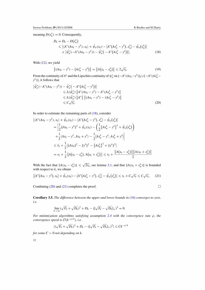
We performed deblurring experiments for a sample image with 256×256 pixels which hasbeen convolved with a circular out-of-focus kernel of 13 pixels diameter and distorted by noise.A spatial discretization of step-size 1 has been chosen; hence, � = [0, 256]2 with the pixelsbeing represented by a translated unit cubes. Finally, the range of greyscale values correspondsto the interval [0, 1]. Note that all errors are measured with respect to this representation.Approximate solutions x(δ) according to definitions 4.1 and 4.2 were computed for a range ofnoise levels δ using the ISTA and MFISTA iterations, see examples 2.9 and 2.10, respectively,with parameters α0 = 0.1, κ = 0.9, τ = 1.1 and σ = 0.25. The outcome of the procedure inthe case of the MFISTA for some representative noise levels δ is depicted in figure 1. It canbe seen that indeed, the procedure yields a reasonable choice of the regularization parameterand the iteration number. The recovered images are sharper on the one hand and neither over-nor under-smoothed, on the other hand. We also observed that visually, the results of ISTAand MFISTA cannot be distinguished, indicating that the method is also robust with respect tothe concrete minimization algorithm utilized in definition 4.1, a hypothesis whose verificationcan also be found at the end of this section.

Figure 2 shows the convergence behaviour, again for the MFISTA realization ofthe algorithm, of the approximation error

∥∥x(δ) − x†∥∥

2 and the regularization parameterα(δ) = αn∗ as δ → 0. Indeed, one can observe that the regularization parameter as well asthe approximation error satisfies some asymptotic rates. In particular, the statement δ2/α → 0of lemma 4.11 can be confirmed. The results also indicate that there is some rate for whichthe approximation error tends to zero. This behaviour can be explained by the results from

27


Figure 1. Reconstructions for different noise levels. Top, from left to right: data yδ for relative noiselevels of 3.4%, 0.6% and 0.1%, respectively. Bottom, from left to right: original data x†, MFISTAreconstructions x(δ) = Bx(δ) from the data in the top row. (Image by Paul Mannix@Flickr [40],licenced under CC-BY-2.0, http://creativecommons.org/licenses/by/2.0/legalcode.)

Figure 2. Left: regularization parameter α versus (absolute) noise level δ. Approximate rateα ≈ 0.0005 δ1.3596. Right: �2-approximation error versus noise level δ. Approximate rate∥∥x(δ) − x†

∥∥�2

≈ 12.1813 δ0.4319. Dotted: computed values, solid: fitted values.

section 5 (see example 5.6 and corollary 5.9) in infinite dimensions, although the concretevalues of η and ζ can, of course, not be obtained as by discretizing, we cut off the wavelet seriesafter finitely many coefficients. Additionally, we performed a quantitative comparison betweenthe ISTA iteration and the MFISTA iteration for the minimization of the respective Tikhonovfunctionals. The comparison admits no significant difference in approximation quality, as canbe seen in figure 3, left. However, the computational complexity can be reduced significantlyby using MFISTA; see figure 3, right. One has to note, nevertheless, that the overall iterationnumber is quite high, in particular, if one wants to obtain highly accurate solutions at lownoise levels.

Finally, as we are using �1-type regularization, one can also examine the sparsity of theobtained solutions, i.e. the number of non-zero wavelet coefficients. Figure 4 shows how the

28

http://creativecommons.org/licenses/by/2.0/legalcode


Figure 3. Comparison of the performance of the two different minimization algorithms, ISTA andMFISTA. Left: reconstruction quality (approximation error). Right: overall number of iterationsteps.

Figure 4. Dashed: number of nonzero wavelet coefficients in the reconstruction x(δ) versus(absolute) noise level. Solid: full number of coefficients of true solution x†.

sparsity develops with respect to decreasing noise levels. The sparsity-promoting effect ofthe regularization functional can be seen quite well here. In particular, in the high noise levelcase, the number of the reconstructed wavelet coefficients is much lower than the full numberof coefficients, which may yield a significant complexity reduction in comparison to the casewhere a �1-type regularization is not utilized.

7. Conclusions

The purpose of the paper was to develop a regularization algorithm which combinesminimization techniques for Tikhonov-type functionals with discrepancy-based a posterioriparameter choice rules. It is based, on the one hand, on computable estimates for thediscrepancy of the exact minimizers in terms of the discrepancy and the primal-dual gapevaluated at the iterates of a given minimization algorithm. On the other hand, adaptivity ofthe regularization parameter as well as stopping is achieved by testing against these estimates.It is worth emphasizing that in this framework, the choice of the minimization technique and

29


of the penalty functional is quite arbitrary as long as they fulfil the set of requirements listedin section 2. We have seen that the procedure establishes a regularization, again under generalassumptions. In particular, for weighted �p-penalty terms, the regularization may also admit aconvergence rate.

Previously, the discrepancy rule has mainly been used either for the parameter choice inTikhonov minimization or for stopping an iterative method. Therefore, our algorithm can beinterpreted as one step in closing the gap between Tikhonov-type regularization and iterativeregularization techniques. Moreover, the functional formulation behind this framework allowsone in particular to estimate the approximation quality of the iterates with respect to the exactTikhonov minimizers. As a side effect, the procedure yields the guarantee that the discrepancyfor the obtained approximate solution as well as the associated exact solutions of the Tikhonovfunctional are within an adjustable bound. Its regularizing effects are independent from theactual minimization algorithm and, consequently, from the number of performed iterations.

We tested the approach with the inversion of the convolution operator within the�p-regularization framework and compared two minimization techniques, the ISTA andmonotone FISTA. As expected, the MFISTA outperformed the ISTA with respect to thecomputational effort, whereas the quality of regularization remained the same. However, thefirst-order minimization techniques seem to be quite slow and an application of higher ordermethods might be useful to speed up the algorithm.

Acknowledgment

KB gratefully acknowledges support by the Austrian Science Fund (FWF) under grant SFBF32 (SFB ‘Mathematical Optimization and Applications in Biomedical Sciences’).

References

[1] Daubechies I, Defrise M and Mol C D 2004 An iterative thresholding algorithm for linear inverse problemswith a sparsity constraint Commun. Pure Appl. Math. 57 1413–541

[2] Beck A and Teboulle M 2009 Fast gradient-based algorithms for constrained total variation image denoisingand deblurring problems IEEE Trans. Image Process. 18 2419–34

[3] Bonesky T 2009 Morozov’s discrepancy principle and Tikhonov-type functionals Inverse Problems 25 015015[4] Anzengruber S W and Ramlau R 2010 Morozov’s discrepancy principle for Tikhonov-type functionals with

nonlinear operators Inverse Problems 26 025001[5] Defrise M and Mol C D 1987 A note on stopping rules for iterative regularization methods and filtered SVD

Inverse Problems: An Interdisciplinary Study ed P C Sabatier (London: Academic) pp 261–8[6] Ramlau R, Teschke G and Zhariy M 2008 A compressive Landweber iteration for solving ill-posed inverse

problems Inverse Problems 24 065013[7] Zhariy M 2009 Adaptive frame based regularization methods for linear ill-posed inverse problems PhD Thesis

University of Bremen[8] Neubauer A 1988 An a posteriori parameter choice for Tikhonov regularization in the presence of modelling

error Appl. Numer. Math. 4 507–19[9] Ramlau R 1999 A modified Landweber-method for inverse problems J. Numer. Funct. Anal. Optim. 20 79–98

[10] Bonesky T, Dahlke S, Maass P and Raasch T 2010 Adaptive wavelet methods and sparsity reconstruction forinverse heat conduction problems Adv. Comput. Math. 33 385–411

[11] Bonesky T and Maass P 2009 Iterated soft shrinkage with adaptive operator evaluations J. Inverse Ill-posedProblems 17 337–58

[12] Raasch T 2009 Sparse reconstructions for inverse PDE problems Structured Decompositions and EfficientAlgorithms (Dagstuhl Seminar Proc. no 08492) ed S Dahlke, I Daubechies, M Elad, G Kutyniokand G Teschke (Dagstuhl: Schloss Dagstuhl – Leibniz-Zentrum fuer Informatik)

[13] Dahlke S, Fornasier M and Raasch T 2012 Multilevel preconditioning and adaptive sparse solution of inverseproblems Math. Comp. 81 419–46

30

http://dx.doi.org/10.1002/cpa.20042

http://dx.doi.org/10.1109/TIP.2009.2028250

http://dx.doi.org/10.1088/0266-5611/25/1/015015

http://dx.doi.org/10.1088/0266-5611/26/2/025001

http://dx.doi.org/10.1088/0266-5611/24/6/065013

http://dx.doi.org/10.1016/0168-9274(88)90013-X

http://dx.doi.org/10.1080/01630569908816882

http://dx.doi.org/10.1007/s10444-010-9147-2

http://dx.doi.org/10.1515/JIIP.2009.023

http://dx.doi.org/10.1090/s0025-5718-2011-02507-x


[14] Hanke M and Raus T 1996 A general heuristic for choosing the regularization parameter in ill-posed problemsSIAM J. Sci. Comput. 17 956–72

[15] Jin B and Lorenz D 2010 Heuristic parameter-choice rules for convex variational regularization based on errorestimates SIAM J. Numer. Anal. 48 1208–29

[16] Ito K, Jin B and Takeuchi T 2011 A regularization parameter for nonsmooth Tikhonov regularization SIAMJ. Sci. Comput. 33 1415–38

[17] Burger M and Osher S 2004 Convergence rates of convex variational regularization Inverse Problems 20 1411–22[18] Resmerita E 2005 Regularization of ill-posed problems in Banach spaces: convergence rates Inverse

Problems 21 1303–14[19] Resmerita E and Scherzer O 2006 Error estimates for non-quadratic regularization and the relation to enhancing

Inverse Problems 22 801–14[20] Hofmann B, Kaltenbacher B, Poschl C and Scherzer O 2007 A convergence rates result for Tikhonov

regularization in Banach spaces with non-smooth operators Inverse Problems 23 987–1010[21] Hein T 2009 On Tikhonov regularization in Banach spaces—optimal convergence rates Appl. Anal. 88 653–67[22] Hein T 2009 Tikhonov regularization in Banach spaces—improved convergence rates results Inverse

Problems 25 035002[23] Neubauer A 2009 On enhanced convergence rates for Tikhonov regularization of nonlinear ill-posed problems

in Banach spaces Inverse Problems 25 065009[24] Neubauer A, Hein T, Hofmann B, Kindermann S and Tautenhahn U 2010 Improved and extended results for

enhanced convergence rates of Tikhonov regularization in Banach spaces Appl. Anal. 89 1729–43[25] Tautenhahn U 1996 Error estimates for regularization methods in Hilbert scales SIAM J. Numer.

Anal. 33 2120–30[26] Ekeland I and Temam R 1976 Convex Analysis and Variational Problems (Amsterdam: North-Holland)[27] Showalter R E 1997 Monotone Operators in Banach Space and Nonlinear Partial Differential Equations

(Mathematical Surveys and Monographs vol 49) (Providence, RI: American Mathematical Society)[28] Bredies K and Lorenz D 2008 Iterated hard shrinkage for minimization problems with sparsity constraints SIAM

J. Sci. Comput. 30 657–83[29] Beck A and Teboulle M 2009 A fast iterative shrinkage-thresholding algorithm for linear inverse problems

SIAM J. Imaging Sci. 2 183–202[30] Griesse R and Lorenz D A 2008 A semismooth Newton method for Tikhonov functionals with sparsity

constraints Inverse Problems 24 035007[31] Daubechies I, DeVore R, Fornasier M and Gunturk C S 2010 Iteratively reweighted least squares minimization

for sparse recovery Commun. Pure Appl. Math. 63 1–38[32] Figueiredo M A T, Nowak R D and Wright S J 2007 Gradient projection for sparse reconstruction: application

to compressed sensing and other inverse problems IEEE J. Sel. Top. Signal Process. 1 586–97[33] Bredies K and Lorenz D A 2008 Linear convergence of iterative soft-thresholding J. Fourier Anal.

Appl. 14 813–37[34] Tikhonov A N, Leonov A S and Yagola A G 1998 Nonlinear Ill-posed Problems vol 1 (London: Chapman and

Hall)[35] Grasmair M, Haltmeier M and Scherzer O 2008 Sparse regularization with �q penalty term Inverse

Problems 24 1–13[36] Engl H W, Kunisch K and Neubauer A 1989 Convergence rates for Tikhonov regularization of non-linear

ill-posed problems Inverse Problems 5 523–40[37] Engl H W, Hanke M and Neubauer A 1996 Regularization of Inverse Problems (Dordrecht: Kluwer)[38] Meyer Y 1992 Wavelets and Operators (Cambridge Studies in Advanced Mathematics vol 1) (Cambridge:

Cambridge University Press)[39] Werner D 1995 Funktionalanalysis (Berlin: Springer)[40] Mannix P 2007 A pair of African penguins, Boulders Beach, South Africa http://www.flickr.com/photos/

paulmannix/552264573/

31

http://dx.doi.org/10.1137/0917062

http://dx.doi.org/10.1137/100784369

http://dx.doi.org/10.1137/100790756

http://dx.doi.org/10.1088/0266-5611/20/5/005

http://dx.doi.org/10.1088/0266-5611/21/4/007

http://dx.doi.org/10.1088/0266-5611/22/3/004

http://dx.doi.org/10.1088/0266-5611/23/3/009

http://dx.doi.org/10.1080/00036810802555474

http://dx.doi.org/10.1088/0266-5611/25/3/035002

http://dx.doi.org/10.1088/0266-5611/25/6/065009

http://dx.doi.org/10.1080/00036810903517597

http://dx.doi.org/10.1137/S0036142994269411

http://dx.doi.org/10.1137/060663556

http://dx.doi.org/10.1137/080716542

http://dx.doi.org/10.1088/0266-5611/24/3/035007

http://dx.doi.org/10.1002/cpa.20303

http://dx.doi.org/10.1109/JSTSP.2007.910281

http://dx.doi.org/10.1007/s00041-008-9041-1

http://dx.doi.org/10.1088/0266-5611/24/5/055020

http://dx.doi.org/10.1088/0266-5611/5/4/007

http://dx.doi.org/10.1007/978-94-009-1740-8

http://www.flickr.com/photos/paulmannix/552264573/

http://www.flickr.com/photos/paulmannix/552264573/

A discrepancy-based parameter adaptation and stopping rule for minimization algorithms aiming at...

Documents

Transcript of A discrepancy-based parameter adaptation and stopping rule for minimization algorithms aiming at...