A Diffuse Interface Model of Transport Limited ...
127
A Diffuse Interface Model of Transport Limited Electrochemistry in Two-Phase Fluid Systems with Application to Steelmaking by David Dussault M. S., Mechanical Engineering (2002) Submitted to the Department of Mechanical Engineering in Partial Fulfillment of the Requirement for the Degree of Master of Science in Mechanical Engineering at the Massachusetts Institute of Technology February 2002 BARKER @ 2002 Massachusetts Institute of Technology MASSACHUSETS INSTITUTE All rights reserved OF TECHNOLOGY MAR 2 5 2002 LIBRARIES Signature of A uthor .............................................. Department of Mechanical Engineering Jan 11, 2002 Certified by. ....................... /7 Adam C. Powell Assistant Professor of Materials Engineering A ccepted by. ... ....................... .................. Ain A. Sonin Chairman, Department Committee on Graduate Students
Transcript of A Diffuse Interface Model of Transport Limited ...

A Diffuse Interface Model of Transport Limited Electrochemistry inTwo-Phase Fluid Systems with Application to Steelmaking
by
David Dussault
M. S., Mechanical Engineering (2002)
Submitted to the Department of Mechanical Engineeringin Partial Fulfillment of the Requirement for the Degree of
Master of Science in Mechanical Engineering
at the
Massachusetts Institute of Technology
February 2002 BARKER
@ 2002 Massachusetts Institute of Technology MASSACHUSETS INSTITUTEAll rights reserved OF TECHNOLOGY
MAR 2 5 2002
LIBRARIES
Signature of A uthor . . . . . . . . . . . . . . . . . . . . . . . . . . . . . . . . . . . . . . . . . . . . . .Department of Mechanical Engineering
Jan 11, 2002
Certified by. . . . . . . . . . . . . . . . . . . . . . . ./7 Adam C. Powell
Assistant Professor of Materials Engineering
A ccepted by. . . . . . . . . . . . . . . . . . . . . . . . . . . . . . . . . . . . . . . . . . . . .Ain A. Sonin
Chairman, Department Committee on Graduate Students

Abstract
Electric Field-Enhanced Smelting and Refining is a process for accelerating the rate of carbon
removal from steel in a steelmaking reactor. It is proposed as an alternative or a complement to
the basic oxygen process. Electrodes are inserted into the metal and slag phases. The carbon
is removed from the steel to form CO gas at the anodic interface, and the Fe2 + in the slag
is removed to form Fe at the cathodic interface. The overall reaction rate is limited by the
transport of Fe2 + to the cathode. To accelerate the reaction, the overall cathode mass transfer
coefficient must be increased, and to do so requires an understanding of the kinetics surrounding
the cathode.
An Fe-FeO-Fe electrochemical system is used as a simplified model of the steelmaking process.
In this project two mathematical models of the system are developed: the classical sharp interface
model and a diffuse interface model. In the diffuse interface model, the Cahn-Hilliard Equation is
extended to include fluid flow and migration of ionized species due to an electric field. The voltage
field is solved for using conservation of charge. Asymptotic solutions and scaling results are
derived to explain phenomena surrounding the cathode. The diffuse interface model is discretized
using the finite-difference method. The resulting system of nonlinear algebraic equations are
solved using a Newton-Krylov solver.
The simplified 2D Fe-FeO-Fe system does not capture all phenomena of the physical slag-
metal system, but does provide a foundation for a more comprehensive model to be developed
in the future. The methodology developed here for coupling transport limited electrochemistry
with transport equations is fundamental in that the extension to more complex systems is limited
only by the development of a free energy model and the knowledge of system properties.
2

Acknowledgements
First I would like to thank my advisor, Professor Adam Powell. Thanks for always taking the
time to answer my questions. When I was your only student and I didn't know where to start
with mostly everything in the lab, you always made time for me. Thanks for being supportive
and trusting my work. When the project took a turn for the worst, you supported my decision
on how we could change things. Your flexibility as an advisor sometimes made things harder
for me in the short term, but helped me to be a better researcher and how to solve long term
problems. You were always more concerned about my well being than the status of the project.
Perhaps the most important thing that I'll take from my time with you is not to lose sight of
humanity when dealing with science.
To Professor McKelliget and Dr. Gerardo Trapaga, thank you for helping me in my transition
into MIT. You introduced me to Professor Powell, and then backed off. Things could have been
allot harder for me. You let me pretty much drop the project that we were working on, so I
could focus on my studies at MIT. I probably couldn't have gotten through my first semester
here without your help.
Raymundo, thanks for your help with thermodynamics. You're a good teacher. I think we
complimented each other well. To my lab mates Robert and Bo, thanks for your help with
Materials Science and your help with the computers. You guys were my best resources. Chris,
we got through are classes together. The study sessions were great. Thanks for the talks too.
Professor Sonin, thanks for agreeing to be my ME reader. Gloria, you could read me like a book.
Thanks for helping me through some tough times.
To my family and friends, thanks for giving me space so I could focus at school. You let
me slip into my own world at school for weeks at a time. I think that I had to do that to get
through things here. Then I'd have some time off and everything would be cool again. I couldn't
be around physically or mentally all the time, and you never held it against me. Thanks.
Last, I would like to thank the NIST Green's function working group for supporting part of
this research.
3

Contents
1 Introduction 10
1.1 Introductory Remarks . . . . . . . . . . . . . . . . . . . . . . . . . . . . . . . . . 10
1.2 Modeling and Simulation . . . . . . . . . . . . . . . . . . . . . . . . . . . . . . . . 10
1.3 Current Steelmaking Method . . . . . . . . . . . . . . . . . . . . . . . . . . . . . 11
1.4 Proposed Changes ...... .. ................................... 13
1.5 Overview of Thesis . . . . . . . . . . . . . . . . . . . . . . . . . . . . . . . . . . . 14
2 Sharp Interface Model 17
2.1 Introductory Remarks . . . . . . . . . . . . . . . . . . . . . . . . . . . . . . . . . 17
2.2 Governing Equations . . . . . . . . . . . . . . . . . . . . . . . . . . . . . . . . . . 17
2.3 Interface Conditions . . . . . . . . . . . . . . . . . . . . . . . . . . . . . . . . . . 20
2.4 Electrochemistry . . . . . . . . . . . . . . . . . . . . . . . . . . . . . . . . . . . . 23
2.4.1 Thermodynamics . . . . . . . . . . . . . . . . . . . . . . . . . . . . . . . . 24
2.4.2 K inetics . . . . . . . . . . . . . . . . . . . . . . . . . . . . . . . . . . . . . 25
2.4.3 Charge Buildup Layer . . . . . . . . . . . . . . . . . . . . . . . . . . . . . 32
2.5 Scaling and Asymptotic Solutions . . . . . . . . . . . . . . . . . . . . . . . . . . . 34
2.5.1 1D Electrochemical System . . . . . . . . . . . . . . . . . . . . . . . . . . 34
2.5.2 Charge Buildup Layer . . . . . . . . . . . . . . . . . . . . . . . . . . . . . 36
2.5.3 Diffusion Limited Growth . . . . . . . . . . . . . . . . . . . . . . . . . . . 38
2.5.4 Capillary Instability . . . . . . . . . . . . . . . . . . . . . . . . . . . . . . 39
4

2.5.5 Buoyancy Instability . . . . . . . . . . . . . . . . . . . . . . . . . . . . . . 39
3 Diffuse Interface Model 41
3.1 Cahn-Hilliard . . . . . . . . . . . . . . . . . . . . . . . . . . . . . . . . . . . . . . 41
3.2 Fe-FeO System . . . . . . . . . . . . . . . . . . . . . . . . . . . . . . . . . . . . . 47
3.2.1 Cahn-Hilliard . . . . . . . . . . . . . . . . . . . . . . . . . . . . . . . . . . 47
3.2.2 Governing Equations . . . . . . . . . . . . . . . . . . . . . . . . . . . . . . 49
4 Numerical Methods 57
4.1 Introductory Remarks . . . . . . . . . . . . . . . . . . . . . . . . . . . . . . . . . 57
4.2 Discretization of Governing Equations, Finite Difference Method . . . . . . . . . . 58
4.3 Symmetry Boundary Conditions, Shadow Nodes . . . . . . . . . . . . . . . . . . . 64
4.4 Nonlinear Solver, Multidimensional Newton's Method . . . . . . . . . . . . . . . . 67
4.5 Krylov Subspace Linear Solver . . . . . . . . . . . . . . . . . . . . . . . . . . . . . 69
4.5.1 QR Factorization, Gram-Schmidt Algorithm . . . . . . . . . . . . . . . . . 69
4.5.2 General Minimization Algorithm . . . . . . . . . . . . . . . . . . . . . . . 72
4.5.3 Krylov Subspace Generation . . . . . . . . . . . . . . . . . . . . . . . . . . 75
4.5.4 The Generalized Conjugate Residual Algorithm . . . . . . . . . . . . . . . 77
4.6 Newton-Krylov Matrix Free Approximation . . . . . . . . . . . . . . . . . . . . . 78
4.7 P E T Sc . . . . . . . . . . . . . . . . . . . . . . . . . . . . . . . . . . . . . . . . . . 79
5 Numerical Simulation Case Studies 83
5.1 Introductory Remarks . . . . . . . . . . . . . . . . . . . . . . . . . . . . . . . . . 83
5.2 D iffusion . . . . . . . . . . . . . . . . . . . . . . . . . . . . . . . . . . . . . . . . . 84
5.3 Diffusion, Migration . . . . . . . . . . . . . . . . . . . . . . . . . . . . . . . . . . 88
5.4 Diffusion, Surface Tension Driven Convection . . . . . . . . . . . . . . . . . . . . 106
5.5 Diffusion, Gravity and Surface Tension Driven Convection . . . . . . . . . . . . . 110
5

6 Discussion
6.1 Introductory Remarks . . . .
6.2 Assumptions and Limitations
6.3 Applications . . . . . . . . . .
6.4 Future Work. . . . . . . . . .
117
. . . . . . . . . . . . . . . . . . . . . . . . . . . . . 117
. . . . . . . . . . . . . . . . . . . . . . . . . . . . . 117
. . . . . . . . . . . . . . . . . . . . . . . . . . . . . 119
. . . . . . . . . . . . . . . . . . . . . . . . . . . . . 120
7 Conclusions 122
8 Appendix 124
8.1 Properties . . . . . . . . . . . . . . . . . . . . . . . . . . . . . . . . . . . . . . . . 124
8.2 ComputerProgram . . . . . . . .. . . . . . . . . . . . . . . . . . . . . . . . . . .124
6

List of Figures
1.1 Slag/metal system . . . . . . . . . . . . . . . . . . . . . . . . . . . . . . . . . . . 1 2
1.2 Slag/metal system with electrodes . .
2.1 Slag/metal Interface . . . . . . . . .
2.2 Concentration profile in slag . . . . .
2.3 Transfer coefficient and free energy .
2.4 Current vs. overpotential . . . . . .
2.5 Current vs. overpotential for different
2.6 Initial voltage profile, 1D system.
2.7 Final voltage profile, 1D system .
2 .8 . . . . . . . . . . . . . . . . . . . . .
2.9 Distorted slag/metal interface . .
2.10 Capillary instability . . . . . . . . . .
3.1
3.2
3.3
exchange currents
Free energy density vs. concentration
Inhomogeneous system . . . . . . . .
Free energy hump . . . . . . . . . . .
3.4 Free energy of Fe-FeO system using sublattice i
4.1
4.2
4.3
. . . . . . . . . . .
... .. .. .. ..
... ... .. .. .
onic liquid model .
Finite difference grid . . . . . . . . . . . . . . . . . . . . . . . .
Finite difference grid . . . . . . . . . . . . . . . . . . . . . . . .
Shadow nodes ...... ............................
7
13
21
26
27
31
31
32
33
35
38
39
42
43
44
48
58
59
65

4.4 ID Newton's method
4.5
4.6
73
. . . . . . . . 80
1D minimization ... ................
PETSc distributed array ..............
Initial concentration profile . . . . . . . . . . .
C at steady state, ID system, 16 nodes . . . .
C at steady state, 1D system, 32 nodes . . . .
C at steady state, ID system, 64 nodes . . . .
C at steady state, 1D system, 128 nodes . . .
Evolution of concentration profile, ID system,
C at t=O, multi-interface system . . . . . . . .
C at steady state, multi-interface system, N=1l
C at steady state, multi-interface system, N=-2
C at steady state, multi-interface system, N=3
C at t=0, applied voltage . . . . . . . . . . . .
C at t=1300s, applied voltage . . . . . . . . .
Voltage at t=1300s, applied voltage . . . . . .
C at t=0, perturbed cathodic interface . . . .
C at t=O, perturbed anodic interface . . . . .
C at t=1660s, perturbed cathodic interface . .
C at t=1660s, perturbed anodic interface . . .
5.1
5.2
5.3
5.4
5.5
5.6
5.7
5.8
5.9
5.10
5.11
5.12
5.13
5.14
5.15
5.16
5.17
5.18
5.19
5.20
5.21
5.22
5.23
5.24
nodes
. . . . . . . . . . . . . . 8 4
. . . . . . . . . . . . . . 8 5
. . . . . . . . . . . . . . 8 6
. . . . . . . . . . . . . . 8 6
. . . . . . . . . . . . . . 8 7
. . . . . . . . . . . . . . 8 7
. . . . . . . . . . . . . . 8 9
. . . . . . . . . . . . . . 9 0
. . . . . . . . . . . . . . 9 1
. . . . . . . . . . . . . . 9 2
. . . . . . . . . . . . . . . . . . . . 94
. . . . . . . . . . . . . . . . . . . . 96
. . . . . . . . . . . . . . . . . . . . 97
. . . . . . . . . . . . . . . . . . . . 99
. . . . . . . . . . . . . . . . . . . . 100
. . . . . . . . . . . . . . . . . . . . 101
. . . . . . . . . . . . . . . . . . . . 102
applied voltage . . . . . . . . . . . 103
)plied voltage . . . . . . . . . . . . 104
C at steady state, perturbed cathodic or anodic interface, no applied voltage
C at t=0, 2D drop . . . . . . . . . . . . . . . . . . . . . . . . . . . . . . . .
Radius (m) 445deg vs time (sec) . . . . . . . . . . . . . . . . . . . . . . . .
C at steady state, 2D drop . . . . . . . . . . . . . . . . . . . . . . . . . . . .
,Radius (m) ©45deg vs time (sec) . . . . . . . . . . . . . . . . . . . . . . . .
. . . 105
. . . 109
. . . 110
111
112
8
32
C at t=1660s, perturbed cathodic interface, no
C at t=1660s, perturbed anodic interface, no a
.. .. ... ... 67

5.25 C at steady state, 2D drop with gravity . . . . . . . . . . . . . . . . . . . . . . . . 113
9

Chapter 1
Introduction
1.1 Introductory Remarks
The objective of this thesis is to develop a mathematical model which describes two-phase
fluid/fluid systems with transport limited electrochemical reactions. There are many appli-
cations for the model. The application described in this paper is a new method for low carbon
steel refining known as the electric field enhanced smelting and refining of steel. In this section,
relevant previous modeling methods are given, and the extension of the current modeling meth-
ods to the system of interest is outlined. Following that is a description of the physical system
along with a brief background to steelmaking. Finally, an overview of the entire thesis is given.
1.2 Modeling and Simulation
The model developed in this thesis is for a two phase isothermal liquid/liquid system undergoing
transport limited electrochemical reactions. In order to avoid interface tracking and interface
boundary conditions, a diffuse interface phase-field model was used. In the phase-field method,
a composition field variable C(x, y, z) varies from 0 in one phase to 1 in the other phase. The
interface spans a finite region and is represented by fractions of C.
The phase-field method is based on the Cahn-Hilliard equation which is a diffuse interface
10

diffusion equation originally applied to spinoidal decomposition [16]. The Cahn-Hilliard equation
was extended to fluid/fluid systems by Jacqmin [9, 10] by using a modified stress tensor to account
for surface tension. A general phase-field model for non-isothermal binary fluid/solid systems was
developed by Sekerka and others in [18]. Papers on phase-field application and theory include
[19, 20, 21, 22]. For a rigorous comparison of diffuse interface and sharp interface descriptions of
fluid systems including heat transfer see Anderson and McFadden [15]. The Cahn-Hilliard free
energy formulation was extended to general multi-component systems by Hoyt [17]. Multi-phase,
multi-component systems are an area of active research.
In this thesis, the diffuse interface model developed by Jacqmin for two phase, two component,
liquid/liquid, isothermal, flow is extended to include transport limited electrochemical reactions.
To couple the transport of chemical species with electrochemistry, a migration term was added to
the diffusion of chemical species equation. The Cahn-Hilliard free energy model allowed for inter-
phase diffusion. Because the electrochemistry is in the transport limited region, the constitutive
exponential current-voltage relations reduce to linear current-mass flux relations which reduces
coupling in the governing equations. The voltage field is solved for using conservation of charge.
Assuming rapid charge redistribution, the conservation of charge equation reduces to an equation
for zero divergence of current flux and implicitly allows for nonuniform charge density.
1.3 Current Steelmaking Method
Steel is an iron alloy consisting of approximately 95 to 99 wt% iron, 0.01 to 2 wt% carbon, and
traces of other elements such as magnesium, phosphorus, sulfur, silicon, nickel, and chromium.
The amount of carbon has a direct influence on the mechanical properties of the steel such as
yield strength and ductility. In general as the percentage of carbon decreases, yield strength
decreases and ductility increases. For example, steel used for tools is 1.35 wt% carbon and steel
used for construction is 0.25 wt% carbon. The process by which steel is derived from iron ore
consists of primarily two steps: the blast furnace and the basic oxygen process. For low carbon
11

Figure 1.1: Slag/metal system
steel, the steel is further processed in what is called vacuum degassing.
In the blast furnace iron ore enters along with lime (CaO), coke (refined coal) and hot air.
The products react over a range of 200 to 2000 degrees C. The exiting products include hot gases
such as CO and C02, molten iron, and molten slag (a mixture of oxide impurities left over from
the iron ores). The density of slag is on the order of 1/2 that of steel. Thus, the slag and steel
separate mechanically. The resulting slag is discarded, while the resulting iron, referred to as pig
iron, is on the order of 5 wt% carbon.
The slag/melt system is shown in Figure 1.1. In the basic oxygen process a jet of oxygen is
applied to the slag layer. The speed of the oxygen gas is such that the slag gets pushed aside
and the gas reaches the iron melt where it combines with carbon to form carbon monoxide.
0 2 (gas) + 2C(metal) -+ 2CO(bubble) (1.1)
However, the oxygen also reacts with the iron in the melt to form iron oxide.
0 2 (gas) + 2Fe(metal) -+ 2FeO(slag) (1.2)
The loss of iron from the melt to the slag is an inefficiency inherent to this method. The presence
of FeO in the slag leads to slag foaming and corrosion of cylinder walls, and the increase in slag
mass leads to environmental issues. Discarded slag contains typically 20 to 25 wt% iron. The
12

Figure 1.2: Slag/metal system with electrodes
resulting steel is on the order of 0.1 wt% carbon.
In the vacuum degassing stage, the carbon content is reduced further. In this stage a vacuum
is pulled over the slag-steel system. Because there is a low partial pressure of CO there is a
thermodynamic driving force for CO bubbles to form and escape (along with traces of all other
elements in the system). The system is not heated during the vacuum stage. Instead, the
system temperature is elevated before the vacuum is applied such that the steel remains molten
during the process. The resulting steel is on the order of 0.01 wt% carbon. The inefficiencies
associated with this step are the energy associated with elevating the steel temperature, the
energy associated with maintaining the vacuum, and the impurity of the CO removed . The
carbon and oxygen must diffuse through a concentration boundary layer to reach the interface
before forming CO. Thus, the process is limited by a diffusion time-scale.
1.4 Proposed Changes
A new process for refining steel known as 'Electric Field-Enhanced Refining of Steel' was devel-
oped by Professor Uday Pal of Boston University [131. The idea behind this system is to generate
CO from the oxygen already in the slag. The proposed system is shown in Figure 1.2. There is
no external supply of oxygen. An external circuit is added to the system. The cathode lies in
the slag phase, while the anode lies in the melt. Because iron is a good electrical conductor, the
entire melt effectively becomes the anode. The FeO in the slag exists in ionic form, Fe2+ and
02-. There are two interfaces where electrochemical reactions occur, the slag/cathode interface
13
..........

and the slag/anode interface. With this configuration there is a thermodynamic driving force
for electrochemical reactions to occur that are consistent with the current through the circuit.
Electrons flow from the anode to the cathode. At the cathodic interface Fe is formed on the
electrode.
Fe2 +(slag) + 2e- - Fe(melt) (1.3)
At the anodic interface CO is formed.
02-(slag) + C(melt) -+ CO(gas) + 2e- (1.4)
Thus, CO is formed without an external supply. The inefficiencies described above are not
present in this process. The Fe that is formed on the cathode falls back into the melt (the
mechanics are described in Chapter 2). Therefore, Fe is recovered from the slag instead of being
lost to the slag, and there is a decrease in slag mass instead of an increase in slag mass.
The current savings associated with this process are as follows. The decrease of 20 wt% FeO
in slag translates roughly into a savings of 179 MJ per metric ton of steel or $2.33 per metric
ton of steel. There are 800 million tons of steel produced per year. Therefore, the total savings
would be 143 * 10"J per year or $1.8 billion per year.
1.5 Overview of Thesis
The physical electrochemical slag/metal system described above is represented throughout the
thesis by a simplified Fe-FeO electrochemical system. Both systems are referred to throughout
the thesis. However, the chapters intentionally display a great deal of independence. The model
developed here builds on previous works, but still does not capture all phenomena associated
with typical applications. The independence is designed to benefit to the development of future
work.
Chapter 2 introduces the classical sharp interface model for general multicomponent fluid
14

electrochemical systems. The conservation equations are given without simplifications. Interface
conditions are derived based on conservation principles. Assuming that the reader is familiar
with thermodynamics, an introduction to electrochemisty is given. Constitutive current-voltage
relations are derived and the transport limited case is shown as an asymptotic limit. Finally,
for the physical slag/metal system, the governing equations are solved for a number of simplified
asymptotic cases giving rise to system length, time, and velocity scales.
Chapter 3 introduces the diffuse interface model for a two component liquid/liquid system
and applies it to the Fe-FeO system. The Cahn-Hilliard equation is derived, and the coefficients
are related to system properties. The phase-field model is derived by scaling parameters in
the Cahn-Hilliard equation while retaining the system's surface tension. The diffuse interface
governing equations are first presented in general and then are applied to the Fe-FeO system.
Voltage is solved using conservation of charge. Given that the system is transport limited and
that there is rapid charge redistribution, a number of terms in the conservation of charge equation
are neglected and the coupling of the equations is significantly reduced.
The resulting system of equations are solved numerically. Chapter 4 describes in detail the nu-
merical methods used. The finite difference method was used for space and the Crank-Nicholson
scheme was used for time. Shadow nodes were used for symmetry boundary conditions. Once
discretized, the system of partial differential equations becomes a system of nonlinear algebraic
equations. Newton's method was used for the nonlinear solver and the generalized conjugate
residual algorithm was used for the linear solver. Together they are commonly referred to as a
Newton-Krylov solver. The solver allows for a finite-difference approximation to the Jacobian
matrix. PETSc (The Portable, Extensible Toolkit for Scientific Computing), a collection of C
libraries, was used for managing data storage and for parallel processing.
Chapter 5 contains numerical simulations of case studies. Each case study is designed to cap-
ture a single phenomenon associated with physical system. The first simulation demonstrates
interface diffusion and the effect that interface scaling has on the output. The second simula-
tion demonstrates diffusion coupled with migration. Interface motion due to an electric field is
15

displayed along with the growth of interface perturbations. The third simulation demonstrates
two phase surface tension driven convection by looking at an oscillating 2D drop. And the
fourth simulation demonstrates two phase surface tension driven convection in the presence of
a gravitational field. The same 2D drop is used, and the interface profile agrees with analytical
calculations.
Chapter 6 and Chapter 7 are the discussion and conclusion respectively. The key assumptions
are revisited. Limitations of the model are discussed. The application of the model to other
physical systems is briefly described. Future development of the model to broaden the range of
application is discussed. Simulation results are summarized.
16

Chapter 2
Sharp Interface Model
2.1 Introductory Remarks
The slag/steel system is represented here by a two-phase fluid continuum. There are two ways of
modeling the system, the sharp interface model (given in this chapter) and the diffuse interface
model (given in Chapter 4). In the sharp interface model the governing equations are applied to
each separate phase, and boundary conditions are set at the internal interfaces. In the diffuse
interface model the governing equations are applied to all phases at once, so boundary conditions
are not needed at the internal interfaces. Of course, for both methods boundary conditions must
be set on the outer surfaces.
This Chapter follows the sharp interface model. First, the governing equations are given for
as general a case as possible. For this reason some modeling which is problem dependent is left
out. Next, a number of instabilities associated with the slag/metal system are described and
asymptotic solutions are derived.
2.2 Governing Equations
The equations that follow are for a two-dimensional, single-phase, compressible, multi-component,
ionic fluid with variable properties. The field variables associated with this system are:
17

1. u, x-component of velocity
2. v, y-component of velocity
3. p, pressure
4. wi, mass fraction of species i
5. q, voltage
6. pf, free charge density (free charge per unit volume of fluid) (this parameter is introduced
below)
Six governing equations are needed. The fluid has a density p, a viscosity '0, and a velocity .
In general there will be a gravitational field characterized by the gravitational acceleration-?.
The first equation is conservation of x-direction momentum.
a(pu) + e (pVu) =at(2.1)
Dx + (nV ) + pg+ax- n eV
The second equation is conservation of y-direction momentum.
(p) + V 0 (PV) = (2.2)-p + (,qvv) + PgyDy
S(V) - 2D a~.V
The first two viscous stress terms in the above two equations follow the familiar diffusion form
and for a fluid with constant properties are the only remaining viscous terms. The other viscous
stress terms are due to variable viscosity and incompressibility. The third equation is conservation
of mass.
18

+ + (pr) = 0 (2.3)at0
The fourth equation is conservation of species.
at(PW) + V (prwi) =M- .(3 ) (2.4)
There is no generation of species in this formulation. The reactions occur at the slag/metal
interface and are introduced through boundary conditions. 7 is the mass flux of species i (units
are '9 ), where the flux is measured relative to the bulk velocity (diffusion flux). The molar
flux of species i I (units are 'l"") is given by [1]
=-D. -zF Diciv# (2.5)
The first term represents diffusion due to concentration gradients, and the second term represents
diffusion due to the effect of an electric field on an ionic component. Here Di is the diffusion
coefficient of species i (units are a), zi is the charge of species i (units are mole of excess
protons per mole of species i, for example, ZFe2+ = 2 and Z 0 2- = -2), F is Faraday's constant
(F = 96485 m , where mole corresponds to mole of excess proton), R is the molar gas constant
(R = 8.314 ), and T is absolute temperature (T = 1900K). Mass flux is related to molar
flux through the molar mass Mi (units are mass of i per mole of i).
i = Mi (2.6)
Therefore, the conservation of species equation becomes
a (poW) + V (pwi) = MiV 0 Djf + + Dicivo# (2.7)at PW}=~ ~vi RT V5
19

The fifth equation is Gauss's Law inside matter, which introduces pf defined above.
v e 7 = p, (2.8)
1 is called the electric displacement, and for a linear media it is related to the electric field
through
(2.9)
where e is the permittivity of the media (units are N*2). Combining gives
S 6 - pf
The sixth and last governing equation is conservation of charge.
Dp c
Dt
The substantial derivative is used to adjust for the transport of charge due to convection. Jc is
the flux of charge (units are ) The charge flux J, is related to the molar flux 7i through
Jc = E J ziF
Combining gives
where ji is given by Equation 2.5.
2.3 Interface Conditions
Dpf-
Dt
First, the velocity interface condition is derived by a mass balance at the interface.
(2.12)
(2.13)
Consider
the slag/metal system shown in Figure 2.1. The interface moves with a velocity Vint. The
20
(2.10)
(2.11)
-V * (E J, ziF)

skag
dh
MetaUconttro(
Area=DettaA volume
Figure 2.1: Slag/metal Interface
unit vector normal to the interface is given by 7, where -# is positive when pointing in the
slag direction. A infinitesimal cylindrical control volume of height dh and cross-sectional area
AA encloses a small portion of the interface. The control volume moves with the interface, so
mass enters on the slag side and mass leaves on the metal side (according to this positive sign
convention). Applying conservation of mass gives
P8iag (Vint - Vstag) # = Pmetal (Vint - Vmetal) # (2.14)
Or, in terms of the normal components of the vectors
Pslag (Vint,n - Vsiag,n) = Pmetal (Vint,n - Vmetal,n) (2.15)
The tangential velocity is given by the no-slip condition.
Vmetal,tangent = Vnt,tangent = Vsiag,tangent (2.16)
21

The normal component of the interface velocity is found by applying conservation of electrons
at the interface. The interface moving through a distance dx during a time dt. A number of
electrons Ne- enter the control volume from the metal, and a number of Fe2+ atoms NFe2+ enter
the control volume from the slag. They are related by
Ne- = 2NFe2+ = 2 ldx+ A (2.17)V ol
Dividing through by dt and rearranging gives
_JVs
Vint,n = (2.18)2F
where V, is the molar volume of slag (units are volume of slag per mole of Fe), and J is the
current density (units are C / unit area / unit time ). There will be a discontinuity in pressure
across the interface due to surface tension. The relation is
AP = o + (2.19)(R1 R2)
Where a is the surface tension and R 1 and R 2 are the principal radii of curvature. The last
interface condition involves pf and #. Writing Gauss's law in integral form
* tdA = Qf,enclosed (2.20)
where Qf,enciosed is the total charge enclosed in the control volume shown in FIGURE. Simplifying
gives
Dn,siag - Dn,metal = Uf (2.21)
where of is the surface free charge density on the interface (units are charge / unit area).
Continuing, there will be a discontinuity in the D field and a corresponding discontinuity in
the E field which would imply a discontinuous gradient on voltage. However the voltage is
22

continuous across the interface. That is,
0 1ag = qmetaj (2.22)
2.4 Electrochemistry
Electrochemistry is the science of chemical reactions involving electron transfer at an interface.
A general electrochemical reaction has the form
O + ne = R (2.23)
where n is called the electron transfer number. The reaction occurs at an electrode/electrolyte
interface. The electrode is an electrical conductor, and the electrolyte is an ionic conductor. The
electrode at which reduction (reduction in oxidation number) takes place is called the cathode,
and the electrode at which oxidation (increase in oxidation number) takes place is called the
anode. Referring to the slag/metal system described in Section 1.4, Fe2+ is reduced to form Fe
on the cathode
Fe2+(slag) + 2e- -+ Fe(melt) (2.24)
and 02- is oxidized to form CO at the anode.
0 2 -(slag) + C(melt) -+ CO(gas) + 2e- (2.25)
The overall chemical reaction of the system is
02- (slag) + C (melt) - CO (gas) + 2e- (2.26)
23

2.4.1 Thermodynamics
In this section energy principles are applied to electrochemical systems in equilibrium. The
resulting equation known as the Nernst equation relates the cell voltage to the concentrations of
each species.
Consider the general chemical reaction
aA + bB --+ cC + dD (2.27)
The free energy change associated with this reaction is
AG = AG+ RTIn aba (A aB)
(2.28)
The free energy is also equal to the work done on the electrons as they pass through the circuit.
AG = -W,e, = -nFe (2.29)
where F is Faraday's constant, and e is the circuit voltage (cell emf). Inserting Equation 2.29
into Equation 2.28 gives Nernst Equation.
o RT aan F aaB
(2.30)
where e0 is the standard potential of the reaction. Considering a non-ideal solution
6 RTnF (a -bAB
RT ([C]c[D]
nF ([Ala[B]b)(2.31)
0, RT In [C[D]nF n[A]a[B]bJ
24

where 30' is called the formal potential. For the general electrochemical reaction,
Eeq = E R In (q) (2.32)nF C 1
2.4.2 Kinetics
In this section constitutive equations are given which describe electrochemical systems that are
not in equilibrium. The resulting equation relates the current through the circuit to the applied
voltage and the concentrations of each species.
Consider the general electrochemical reaction
0 + ne # R (2.33)
The arrows are used to emphasize the idea that the system is not in equilibrium. Instead forward
and backward reactions are considered to be happening simultaneously.
vf = kfCo (2.34)
Vb = kbCR (2.35)
Vf and Vb are the reaction rates in the forward and backward direction (units are M), kf and
kb are rate constants (units are ,), and Co and Ca are the the concentrations of each species at
the interface. The net reaction rate is given by
Vnet = Vf - Vb = kfCO - kbCR (2-36)
If the system is in equilibrium, then Vnet = 0
Vnet = 0 = k _C - kbCe -+ kfC = kbC%' (2.37)
25

C0(xt)
Figure 2.2: Concentration profile in slag
The reaction rate at equilibrium is called the exchange velocity vo.
(2.38)vo = kfCO = kbCR
The reaction rate is related to current by using Faraday's Law.
l dN I d (Q )A dt Adt nF}
inFA
(2.39)
Consider the one dimensional profile shown in Figure 2.2. The rate of forward reaction is given
by
Vf = kfCo (x = 0,t) = icathodicnFA
(2.40)
and the rate of backward reaction is given by
vf = kbCR(x =Ot) = Zanodic
nFA
26
(2.41)

olpha=I/2 cnhal/opphah/2C C C c~h~/
D+ne W +ne D+neF r Qj Td
L L
-a~
d d 05ka = kx R 7 R£ C
Reaction) Coordinate Reaction Coordinate Reaction Coordinate
Figure 2.3: Transfer coefficient and free energy
The rate constants are related to the voltage by
0 anFekf = f kexp (- 4e) (2.42)
kb = k exp ((1 - C) (2.43)b ~RT)
where ko and ko are the rate constants at e = 0 for the voltage scale in use, and a, the transfer
coefficient, is a measure of asymmetry of the activation barrier of the free energy curve of the
reaction. The effect of a is shown qualitatively in Figure 2.3. If the system is in equilibrium
and the solution is such that C = C, then the Nernst Equation gives e = 6''. Under these
conditions 2.37 becomes
kC_7 = kbCR' - k = kb (2.44)
Using Equations 2.42 and 2.43
exp - =nFE ko exp (1- a) ' k (2.45)koep RTO RT
where ko is called the standard rate constant. Therefore, ko = kf (6o') = kb (Eo'). Inserting the
above equation into Equations 2.42 and 2.43 gives
k = ko exp -aRF (E o )) (2.46)
27

kb = k exp (1 - a) R(e-eO)) (2.47)
The positive sign convention for the net current is the cathodic direction.
i = icathodic - ianodic (2.48)
Using Equations 2.40 and 2.41
i = nFAkf Co (x = 0, t) - nFAkbCR (X = 0, t) (2.49)
Using Equations 2.46 and 2.47 gives the complete current voltage characteristic of the electrode.
i = nFAk0 C0 (x = Ot) exp (-a (e-o' (2.50)
-nFAkCR (x = 0, t) exp ((1 - a) I(e - ,'
At equilibrium the current-voltage relation should reduce to the Nernst Equation. At equilibrium,
i = 0, CR (0, t) = C*, and Co (0, t) = C . The equation reduces to
C* exp (- cr 2 (eeq - e')) = C* exp ((1 - a) (eeq -(E '(2.51)
=> exp (jF --0 = (2.52)
which is an exponential form of the Nernst Equation. Therefore, as the system approaches
equilibrium the kinetic model agrees with the laws of thermodynamics.
Now, the current-voltage relation will be written in terms of exchange current and overpo-
tential. The exchange current io is defined as the magnitude of the cathodic or anodic current
at equilibrium.
io = nFAkC exp - (e, -o (2.53)
28

Raising equation 2.51 to the power -a and combining with the above equation gives the final
equation for exchange current.
io = nFAkOCg'-")Ci (2.54)
Overpotential 7 is defined by
= - 6 eq (2.55)
Dividing equation 2.51 by equation 2.54 gives
i CO (x= 0,t) Cb* anF o,- = -t exp - e-eO' (2.56)i0 Cb C RT
CR (X = 0,t) C ~ nF ctC* hep 1a RT
Using equation 2.52 gives the final equation.
i -Co (x = Ot) / ( anF,, CR (X = 0, t) ex (1a nFq \257
exp( T Z Ci exp (1 -a) Rr(2.57)
Now, the current-voltage relation will be written in terms of limiting current. Limiting
current is the current associated with a mass transfer limited reaction. Here migration effects
are excluded, and steady state is assumed. Referring to Figure 2.2, the flux of 0 to the interface
in terms of the mass transfer coefficient mo is
vmt = mo (C; - Co (x = 0)) (2.58)
Using equation 2.40
= mO (C - Co (x = 0)) (2.59)
The largest flux or reaction rate allowed by mass transfer is when Co (x = 0) = 0. Therefore,
29

the cathodic current of a mass transfer limited reaction is given by
ihmiting,cathodic = i,c = nFAmOC (2.60)
Combining equations 2.59 and 2.60 gives an expression for for surface concentration
Co (x = 0) (2.61)
Similarly, for the anodic current
= -- MR (CR - CR (X = 0)) (2.62)nFA
itimiting,anodic = ii,a= -nFAmRCR (2.63)
CR (X=0) i 2.4CR 1i,a
Using equations 2.60 and 2.64, the current-overpotential equation becomes
- = - exp -_ - - -- ) exp ((1 - a) n ) (2.65)ZO ic RT kia RT
Solving for i
exp (-F q) - exp ((1 - a) 26)i_ =TR (2.66)
-exp ((1 - a) nF
This equation is plotted in Figures 2.4 and 2.5.
In Figure 2.4 , , and - are plotted vs 77 for si,c =-il,a = it, a = 1, n = 1, T = 298K,
and a = 0.5. The solid curve is the total current, the dashed curve is the cathodic current, and
the dotted curve is the anodic current. At large positive overpotential the cathodic current is
negligible, and at large negative overpotential the anodic current is negligible. Near equilibrium
at 7 = 0, the cathodic and anodic contributions are the same order of magnitude. As |9q increases
the system is moved further from equilibrium, and the current increases until it is limited by
30

-0.3 -0.2 -0.1 0etavolts
0.1 0.2 0.3 0.4
Figure 2.4: Current vs. overpotential
-0.3 -0.2 -0.1 0etavolts
0.1 0.2 0.3 0.4
Figure 2.5: Current vs. overpotential for different exchange currents
31
0.8
0.6
0.4
0.2
-0.2
-0.4
-0.6-
-0.8-
-1-0.
- Total current- Cathodic current
- Anodic current
.-
7
- i~'it=10- - '~'il=1.... ~it=0.1
- 0/11=0.01
0
0.8
016 -
0.4 -
0.2 -
S 0
-0.2 -
-0.4-
-0.6-
-0.8
-1 --0.4
I
ami' I4

rmetol SIQ9 rmptak
votge
rhoc=O
Figure 2.6: Initial voltage profile, ID system
mass transfer. In Figure 2.5, j is plotted vs. 17 for various values of A. As Q increases for a fixed
,q the current increases. Or, as A decreases a larger q is required to reach the limiting current.
2.4.3 Charge Buildup Layer
During the initial stages of an experiment there is an inhomogeneous distribution of current
and charge is seen to build up near the interface in a very thin region on the order of 10- 0 m.
To explain the formation of net charge buildup at the interfaces, consider the metal-slag-metal
electrochemical system shown in Figure 2.6. For simplicity, there is no flow, mass transfer is
by migration only, and the system has a uniform permittivity E. The governing equations are
conservation of charge
Pc a (= o (2.67)Ot Ox Ox]
and Gauss's Law
0= 2 + - (2.68)Ox2 6
At t = 0, a voltage is applied to the system. The system initially has homogeneous charge
neutrality. At small times pc = 0, and according to equation 2.68 there will be a linear voltage
32

Mt1Stag MetaL
vA t
Figure 2.7: Final voltage profile, 1D system
profile. The flux of charge is given by
Je (W = 0- ( a) (2.69)
In general omtt>> (781ag,7 so at small times Jc,metal > > Jcsa.Charge (or a deficiency of
electrons) will accumulate at the first interface, and there will be a net loss of charge at the
second interface. The local charge densities will produce local electric fields which at the first
interface lead to a decrease in the rate of incoming charge and an increase in the rate of the
exiting charge and at the second electrode lead to an increase the rate of incoming charge and a
decrease in the rate of exiting charge. A the same time, electrostatic forces act to bring negative
charge to the slag side of the first interface and positive charge to the slag side of the second
interface. At steady state Jc,metal = Jc,,Iag, SO 2 will be nonuniform. The final profiles are shown
in Figure 2.7.
33

2.5 Scaling and Asymptotic Solutions
It has been experimentally shown that when iron is reduced on the cathode, it does not grow out
in an orderly fashion. Instead it grows out and forms liquid dendrites or fingers. The fingers are
approximately cylindrical with a length of 1-4 mm and a diameter of 1/4 mm. The iron fingers
are then shown to break off and fall back into the melt. In this section simple analytical results
are derived which explain this phenomena.
2.5.1 1D Electrochemical System
To first gain some insight into the cathode dynamics consider a ID metal/slag electrochemical
system with constant properties under a constant external electric field -40. Here, conservation
of species is applied to Fe2 + only, so subscripts are excluded. Referring to Equation 2.5, the
total molar flux (diffusion plus convection) of species is given by
-Dv - zF Dcvo + cu (2.70)RT
There is no bulk fluid motion in the slag or the metal. The speed of the interface in the positive
x-direction is given by U, see Figure2.8. Therefore, relative to a coordinate system moving with
the interface, the total molar flux becomes
-Dvc - zF Dc# - cU (2.71)RT
An additional simplification is that relative to the moving interface, the system is in a steady-
state. Conservation of species gives
d2 C ziF d$ dc d2 c dcdx 2 RT dx dx= dx 2 dx (2.72)
34

.g. -U
VIn=0
Figure 2.8:
where A is a constant. The boundary conditions are
c(x = 0) = 0
c (x -+ oo) -
The solution is given byc (x)(
Cbulk- e-A )
which gives a diffusion length scale of
1Ldif ~
The interface velocity is given by Equation 2.18
Jv, (0.5- 2) (14) _4 mmU=-- 2 ~(5m 3.9 * 102F 2 (96485 mote
35
Cbulk
(2.73)
(2.74)
(2.75)
(2.76)
StUton-y C-odinat. Syst-r M-vIng C-odnet. Syst..
ea sA0, -=0
Vimt=U

A closer look at A shows that it can be decomposed into a term due to the electric field and a
term due to the diffusion limited growth of the interface.
zF d4 UA= do + (2.77)RT dx D
zF do 2 (964852vAEfield = zF 2 1 2.4mm' (2.78)
RT dx (8.314 *K) (1900K)
U (3.9 * 10-4mm)Agwth= ~ ( - 1-6 ~- 3.9mm~1 (2.79)
The effects are shown to be of the same order of magnitude. Finally, the diffusion length scale
1 1Ldiff ~ - ~ ~ 0.16mm (2.80)
A 3.9mm-1 + 2.4mm-1
2.5.2 Charge Buildup Layer
In this section a somewhat quantitative explanation of the charge buildup layer is given using
simplified governing equations and scaling arguments. For a more rigorous explanation see the
Gouy-Chapman model [1].
For simplicity, consider a liquid Fe-FeO system with no flow, with mass transfer by migration
only, and with a uniform permittivity E. The governing equations are conservation of charge
=Pc a (o (2.81)at Ox ax~
and Gauss's Law
0 = + - (2.82)Ox2 c
The charge buildup is characterized by a length scale L. In the charge buildup layer the two
36

terms in Gauss's law are the same order of magnitude.
(92 0
Solving for L gives
Pc AO Pc
Pc
Using the bulk concentration of Fe in FeO, c* ', as an estimate for charge density, the open circuit
voltage as an estimate for the voltage difference, and the e co
(0.2V) (8.854 *
(4.983* 104) (
10-12 2)
2) (96485 C)
The time scale for the charge buildup layer to form is given by r. As the charge buildup layer is
forming the terms in equation 2.81 will be the same order of magnitude.
-- 1. ~ u -Ot Ox Ox)
Using equation 2.83 to eliminate Pc
pcL 2
UA~
Recall the molar flux is given by
1i = -D ci -ziF Diciv4RT
Therefore, the conductivity of the slag is
OFeO(ZFe2+F) 2
RT DFeCe
(2.83)
(2.84)
L C~ ~cFeZF e 2+F
~ 10-m (2.85)
Pc _A cTZ24 pc L 2
T L2 OzA
L2)
(2.86)
(2.87)
(2.88)
(2-89)
37
L 2

sig
Figure 2.9: Distorted slag/metal interface
(2)2 (96485 m )2 (10-10m') (4.983 * 104 m1~ol ~e 11.7
(8.314* mol*K) (1900K) l *M
In contrast, OFe =7 * CO5 Continuing, using e e EO and the conductivity of the slag, the
time-scale becomes
EO 8.854 * 10-12 C2
_r_ N*m2 10-12 (2.90)UFeO 11-7n~
The length scale and time scale calculated here are very rough estimates and could be off by a
factor of 10 or so. However, if the values are so extreme that they are many orders of magnitude
different than other length and time scales of interest (as is the case here and as will be displayed
later), then the rough estimates are sufficient.
2.5.3 Diffusion Limited Growth
The initial distortion of the interface into fingers is characterized by a balance between surface
tension and mass transfer. Consider the slag/metal system shown in Figure 2.9. Since the system
is limited by the transport of Fe2+ to the cathode, a diffusion boundary layer will develop in the
slag. Given an initial interface perturbation there will be a local change in the boundary layer
thickness Ldiff, and since the mass transfer to the interface in inversely proportional to Ldiff ,
D (CbuIk - Cinter face) (2.91)j D Ldf f (.1
there will be a corresponding additional local change in interface distortion. For example, at a
point where Ldiff decreases due to a perturbation, j will increase which decreases Ldiff and so
on. Now, as the fingers start to grow surface tension forces act to smooth out the interface. The
balance between the two forces was studied by Mullins and Sekerka t4, 5]. If the length of the
system is larger than the length of the finger spacing as is the case here, then surface tension
38

Figure 2.10: Capillary instability
forces are not strong enough to eliminate the perturbation, and fingers will form.
2.5.4 Capillary Instability
As the fingers form on the cathode they have been shown to break up into droplets. This can be
explained is by surface tension forces. A finger is modeled here as a cylinder of metal surrounded
by an infinite supply of slag (see Figure 2.10). . There will be a higher pressure inside the
cylinder due to surface tension. Given an initial perturbation on the cylinder walls there will be
a corresponding pressure change given by Equation 2.19.
1 1 1 N= + - ~M~~ 8 * 103 2(2.92)
P (R1 R2 ) Rlocal,cylinder mm) m
Now, at regions where the local radius is smaller there will be a larger Ap, and in regions where
the local radius is larger there will be a smaller Ap. Flow will be induced from regions of high
pressure to regions of low pressure. As the cylinder changes shape due to induced flow the
pressure changes are magnified ultimately leading to the breakup of fingers into droplets.
The capillary instability is more formally known as a Rayleigh instability. Rayleigh's analysis
shows that non-axisymmetric modes decay and axisymmetric modes larger then the perimeter
grow. Thus, the wavelength of oscillations is equal to the cross-sectional perimeter 27rR.
2.5.5 Buoyancy Instability
Large drops of metal has been shown to fall from the bottom of the cathode. These drops are
on the order of the finger lengths. They are not droplets from single fingers. Rather, they are
groups of fingers that join and fall together. This can be explained by gravitational forces. The
metal at the bottom of the cathode is modeled as a perfect hemisphere. A force balance between
gravity forces, pressure forces, and surface tension forces gives an order of magnitude for the
39
... .... ......
droplet radius
Ap1 (4 7rR3) g = -y (2irR) (2.93)
37312
')R 3 (~1)-~m 9.3mm (2.94)F2 p-9 \ ( ) (9.81m)
which lies within the expected range.
To find the speed at which a drop falls, the falling metal drop is modeled as a solid sphere
falling in a stationary slag fluid under steady laminar conditions. A balance between gravity
forces, pressure forces and drag forces gives
(Pmetal - Psiag) g (7rR) = fdrag pstagV 2) (7r R2) (2.95)
where fdrag is the drag coefficient. For laminar flow
fdrag = = 24 islag (2.96)ReD \pstagV2R/
Combining gives
(Pmetal - Pag) g (3rR) = 24 ( /2Ra (2 (7rR2\ (2.97)
PsIagVR Psa
Solving for V
2 (Pmetal - Psag) gR 2 2 ( ) (9.81) (mm cm (2.98)V 89 2a (8.1(29 8
M*S,
40
Chapter 3
Diffuse Interface Model
3.1 Cahn-Hilliard
The free energy of a typical phase-separating solution is shown in Figure 3.1 where f is the
free energy density (free energy per unit volume of solution) and C is a dimensionless intensive
measure of concentration (C will be normalized such that it is a dimensionless parameter which
is 0 in phase 1 and 1 in phase2). The two equilibrium phases are c1 and c2 . The Free energy
of an inhomogeneous system (a system with concentration gradients) is assumed to be close to
that of a homogeneous system. Therefore, the free energy of an inhomogeneous system is found
by using a Taylor series expansion of the free energy about the homogeneous state [23].
finh KC VC) = f (C, 0) + L VC + -'C [K] VC + --- (3.1)
where
L = f (3.2)
and
K. - 02 f (3.3)exi ioxjo g(
41
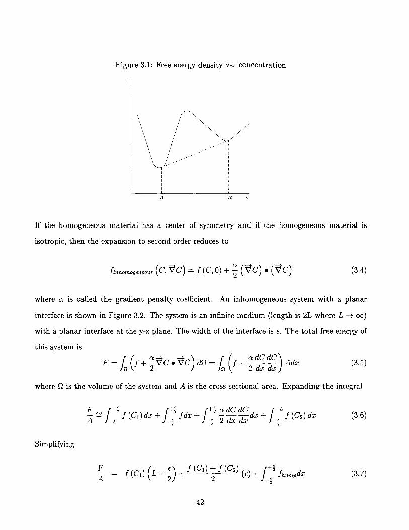
Figure 3.1: Free energy density vs. concentration
C1 C2 C
If the homogeneous material has a center of symmetry and if the homogeneous material is
isotropic, then the expansion to second order reduces to
finhomogeneous (C, VC) = f (C, 0) + (VC) . (VC) (3.4)
where a is called the gradient penalty coefficient. An inhomogeneous system with a planar
interface is shown in Figure 3.2. The system is an infinite medium (length is 2L where L -+ oc)
with a planar interface at the y-z plane. The width of the interface is f. The total free energy of
this system is
F = f + ' C C) d = f + Adx (3.5)
where Q is the volume of the system and A is the cross sectional area. Expanding the integral
F - ++L+dCdCLA- f (C1) dx + f dx + 2 a-j----dx + f (C2) dx (3.6)A -T -- 2 dx dx
Simplifying
F / f (C1) + f (C2) +2=F f (C1) L (2(+ W2 ) + fumpdx (3.7)A f(O 2
42

Figure 3.2: Inhomogeneous system
Ii
4f(C2)
/ I C2
F(C1)
C1
-eps/2 0 eps/2 x
adCdC2 dx dx
+ 2(L) + fhumpdx +'2
[adCdC-2dx xdx + f (C2) (L)
22 xd
where referring to Figure 3.2Fhump f+
A J2 fhumpdx (3.9)
To simplify the analysis let C be a dimensionless parameter which has a value of 0 in phase 1
and 1 in phase 2.C - C1
C2 - C1
The free energy density associated with the hump is modeled with the polynomial T (C) as
shown in Figure 3.3.
fhump = #T (C) = #C2 (1 - C)2
# is a scaling coefficient related to the peak of the free energy curve.
fpeak = /3 4!max = #xy1 1#6
=~2 li=>U=
43
+f+ 2;
= f (C1) (3.8)
(3.11)
16fpeak (3.12)
(3.10U)
+ f (C2) L -
f(C)
f'Peak
psK(C)
C1 C2 C
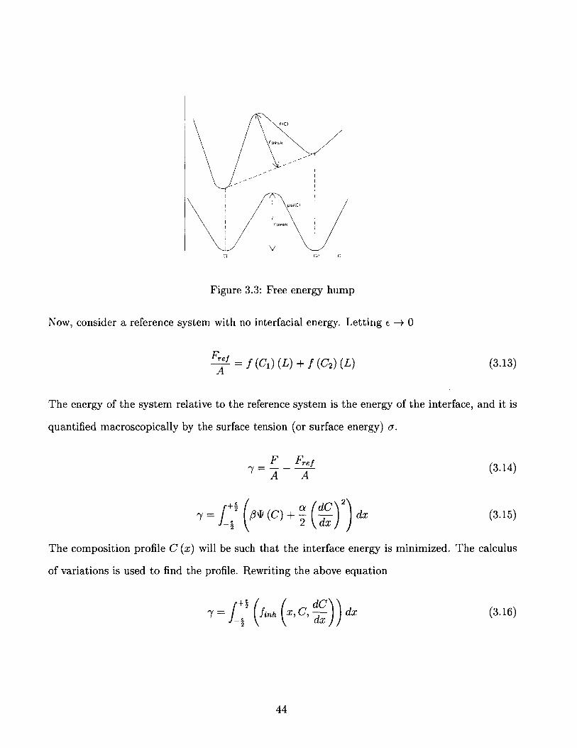
Figure 3.3: Free energy hump
Now, consider a reference system with no interfacial energy. Letting f -+ 0
Fref = f (C1) (L) + f (C2) (L) (3.13)A
The energy of the system relative to the reference system is the energy of the interface, and it is
quantified macroscopically by the surface tension (or surface energy) o.
F Fref (3.14)A A
=q (C) + 2j 9d) dx (3.15)
The composition profile C (x) will be such that the interface energy is minimized. The calculus
of variations is used to find the profile. Rewriting the above equation
= 2 ( finh xC, dx) ) dx (3.16)2.L(d
44

According to Euler's Equation, the function that minimizes the above integral obeys
d (&finh
dx dx ) _ finh = 0aC
(3.17)
(3.18)
Simplifying gives
d ( dC)dx k dx)
dTdC
The left hand side physically represents the local increase of free energy density due to a local
addition in composition 6C (x). Multiplying through by 4 and integrating
dC d ( dC)dx dx k dx
d (adx 2
a (dC )2
2 dx
dT dC-dC dx
dq 0
dx
(3.19)
(3.20)
(3.21)= OT + const
dC = 0 and T = 0, so const = 0.
a (dC 22 dx}
The analytical solution is
d C -A[20: IT+dxtaa
1 1 (X 2/3-+ tanh
L22 2n
Combining Equations 3.22 and 3.15, the surface tension becomes
(231 (0)) dx =+
= > C= 2aOidC
f C2Cli
1(23xw (0)) jcdC
dx
-2aO fv ' dC
45
At C= C1
(3.22)
(3.23)
(3.24)
(3.25)
C (x) =
(dCdx

Solving for alpha
a = - /ii2 C)20 (fgs YidC)2
= 18y 2
20 (1)2
2
The analytical solution gives C (x -+ oo) -+ 1. The interface width can be approximated with
C 6)O0.9
+ 1 tanh (E -222 4v a )
E = 4 2 -tanh-' (2 (0.9-
=0.9
1)
(3.27)
(3.28)
(3.29)c-- 3. 1 r3
In general the flux of species is proportional to the gradient in chemical potential pu.
Ji = -Kiii
where n is the mobility (similar to the diffusion coefficient). For a homogeneous system
(3.31)
(3.30)
Consistent with the above analysis the chemical potential for an inhomogeneous system is defined
by
(3.32)dO
Note that the units of pi are joules per unit volume as opposed to the tradition units of joules
per mole. Therefore, to give molar flux ni has units of m'"*'
Ki in general is a function of composition. At the homogeneous equilibrium compositions,
C1 and C2 the flux reduces to the traditional constitutive equation. For example using the
concentration at phase 1,Dci
Ji = -D ax= (- dC )
46
(3.26)
(3.33)
Ai G
O )Tp,n,:t-ni

D, - (d)C (3.34)19X dC dC ax
Recalling the definition of C
C = 1 00 9 1 - 1= (3.35)c2 -c 1 aX c2 -c 1 x
Combining gives__Di (c2 -- ci)
Ki (C = 0) = (3.36)(q)C=o
where Di is the diffusion coefficient of species component i in phase 1.
In summary, the parameters of the Cahn-Hilliard equation are
# = 16 fpeak (3.37)
a = 187 2 (3.38)
e 3.1 (3.39)
-i (C = 0) =C ) (3.40)(d*C=o
3.2 Fe-FeO System
In this section a mathematical diffuse interface model of the slag-metal system is presented. The
metal phase is modeled as pure Fe, and the slag phase is modeled as pure FeO. The system is at
1900 K.
3.2.1 Cahn-Hilliard
A free energy function for the Fe-FeO system was developed using the sublattice ionic liquid
model from CALPHAD [11]. Gibb's free energy is plotted as a function of XFe in Figure 3.4.
Since the free energy hump is all that is needed for the Cahn-Hilliard equation, the reference free
47

Gibbs Free Energy of Fe-FeO solution at T=1600 degC16000 ---
14000-
12000-
10000-
8000-
4000 --
2000 --
0 --
0.5 0.55 0.6 0.65 0.7 0.75 0.8 0.85 0.9 0.95 1XFe
Figure 3.4: Free energy of Fe-FeO system using sublattice ionic liquid model
energies were set to zero. The figure shows a peak free energy of approximately G 2 14, 000 m
at XFe 2 0.68. The peak in free energy in terms of free energy density is
a and / become
# = 16fpea = 2.72 * 1010 3 (3.42)
_18y2
a = 6.6 * 10- 10N (3.43)
which gives an interface width of
C C 3.1 =4.8 *10-10m (3.44)
To track a one dimensional interface of this thickness on a solution domain on the order of 1cm
would require on the order of 107 grid points. With such extreme length scales, modifications
must be made to the diffuse interface model for practical use.
The interface width is a function of fpeak and -y. To scale the interface, one of these physical
parameters must be altered. In this project fpeak was altered. c was set according to the grid,
48

and 3 was found as a function of E. In terms of E, a and 0 become
3= ((18) (3.1))
(3.45)
(3.46)
This type of scaling is commonly called the phase field method.
3.2.2 Governing Equations
The equations given in this section are similar to the equations given for the sharp interface
formulation. See Section 2.2 for a more detailed description of variables and terms. The Navier-
Stokes equations were extended to the phase field model (see Jacqmin [10]) by adding an extra
surface tension term. Conservation of x-direction momentum reads
a(pu)+ .(pfu) = - 9e(Piu)+pgx
+ V )
- ax f V) - C9
(3.47)
and conservation of y-direction momentum reads
a (PV) + V (pv) = -p + 9 (77u) + pgy
-2
-
49
(3.48)

Conservation of mass is given by
(pVTe+ a p (pe) = 0
The transport equation for conservation of iron is
+V6 (PVFe ) = -MFeVS (IFe) (3.50)
where the molar flux is given by
J-+ =ZFeF DFPWFe V$JFe = KFeViejFe -RT MFe(3.51)
The conductivity of ferrous ions UFe (not to be confused with the electrical conductivity of iron)
is defined by
tcharge,Fe = O'FeP = ~~Fevo (3.52)
and is related to molar flux by
Icharge,Fe ZFeFIFe : IFe ~- _Fe
\ZFeF) V (3.53)
Comparing this result to equation 3.51 gives an expression for the conductivity of ferrous ions
ZFeF DFePWFe
RT MFeUFe - FeF2 DFe,slag PWFe
RT MFe
Combining gives
(PWFe) + VO (PVWFe) = MFeV Y
Recall the chemical potential was given by 3.32
(PWFe)
(3.49)
OFe
ZFeF
a
(3.54)
(KFeVPFe +zFe (3.55)
dOAi = dC _aV 2C
50
(3.56)

C is defined here as
C WFe - WFe,slag
WFe,metal - WFe,slag
=> WFe = (Fe,metal - WFe,slag) C + WFe,8lag = AWFeC + WFe,slag
In terms of C the left hand side of equation 3.55 is
a (PWFe) WFe
* aj (PWFe) + V* (PVWFe)
~ [p (W FeC + WFe,slag)]
+ [PV (/AWFeC + WFe,slag)]
= WFe (p(
+WFe,slag
The second term is zero by the continuity equation. Writing equation 3.55 explicitly in terms of
C gives the final form of the conservation of iron equation.
+Ve (pVC) = MFe
AWFeKFe (TI dO
-C V2C) (3.61)
where the functional dependence of UFe and ZFe on C has been indicated. Note that cFe depends
on C through ZFe and WFe. The mobility is assumed to be constant and given by equation 3.36
KFe = KFe (C = 0) =DFe,slag (CFe,metal - CFe,slag)
d2*) c=o
Note that since C = 1 is pure Fe, kappa is irrelevant at C = 1. ZFe (C) is the charge of Fe
51
(3.57)
(3.58)
(3.59)
(3-60)
- (PC)at
+ MFe O'Fe __
AWFe ZFe (C) F
(3.62)
) + V 0 (PVC)]
(P) + V 0 (Pr)]

atoms (and ions) per mole of Fe atoms (and ions).
ZFe (C) = ZFe2+NFe2+NFe2+ + NFeo
and using the mole fraction relation
XO + XFe = 1
ZFe (C) = 2(1 - XFe ())XFe (C)
Conservation of charge was given by equation 2.13
Dpf _ VzF)
2 XFe2+ _ 2 XFe2+
XFe2+ + XFeO XFe
where NFe2+ is the number of Fe2+ ions, NFeO is the number of neutral Fe atoms.
ZFe2+ = 2, but ZFe varies from 0 in metal to 2 in slag. Assuming charge neutrality
Expanding the right hand side,
DpfDt
=-V* (IFeFZFe (C) + itoFzo+ Icharge,e) (3.68)
For a multi-component system where the velocity is defined by the mass average velocity, the
sum of the diffusion mass fluxes is zero.
MFeIFe + MOO = 0 =>- = - MFe FeMO
(3.69)
52
(3.63)
Note that
2 XFe2+ - 2X 0 2- = 0 -' XO = XFe2+
gives
(3.64)
(3-65)
(3-66)
(3.67)

Eliminating lo from the above two equations gives
DpfDt
=Y - 1 FeFZFe (C) + (- Fe) Fzo + icharge,e) (3.70)
= - (7IFeF [ZFe (C) MFe 40] + Itcharge,e
For convenience let i (C) be defined by
MFe (3.71)
Note that because ZFe > 0 and zo = -2, i (C) > 0. The flux of charge due to electrons is given
by
Icharge,e = Ole (C) IP = -Oe (C) Vq5
where ge reduces to zero in the slag. Conservation of charge becomes
Dpf -V * ((C) F IFe ~ Oe (C) eq)
The molar flux of iron is given by
FeIFe = IiFeV/Fe - Fe (C)ZFe (C) F
Combining gives
F (-KFe I1 Fe -O-Fe (C) g
ZFe (C) F 9) eIUV)
Simplifying,
DpfDt
= o((C)F FeJ Fe) +VFe (
+V 0 (Oe (C) VO)
(3.72)
(3-73)
Dp=Dt
(3.74)
(i(c) (3.75)
(3-76)
53

Charge density exists only at the interfaces, or more generally where the conductivity changes.
Recall from equation 2.90 that the timescale for charge accumulation at the interfaces is on the
order of T-DL - 10-12s. The timescale of interest here is that of bulk fluid motion and diffusion of
species. A physical timescale of interest for the macroscopic system can be obtained from scale
of the interface velocity (equation 2.76) and the diffusion boundary layer (equation 2.80).
LbI 0.16mmTmacro,interest ~' ~ 4 * 016m = 400s (3.77)
Uint 4S 0-M
A timescale for a mesoscopic system would be that associated with the oscillating of a small
droplet due to surface tension forces. Consider the following simplified model. A hemisphere of
radius R initially at rest is pulled through a distance R, by a surface tension force. the equation
of motion is
F = ma => 727rR = p47rR3) 2) (3.78)
Using properties of liquid iron and R = 1mm,
p(R 3 (7160 ) (1mm)3Tmeso,interest = ~3~ 3 * 10-3s (3.79)
The analytical result for an oscillating drop with y = 0.03[, p = 1000I and R ~ 1cm is a
frequency of f ' 50Hz, so the above order of magnitude for an small oscillating iron drop seems
reasonable. The main point is that the timescale of the electrical effects in the charge buildup
layer are microscopic with respect to the system. Therefore, the conservation of charge equation
is effectively at steady state and the unsteady term is neglected.
V * Vp = 1* (i (C) F ,Fe IFe) 0 (Z e (C)Fe (C) (3.80)
+V 0 (ce (C) e )
The dimensionless parameter N, is defined to measure the ratio of the order of magnitude of a
54

convection term to an electric field term.
evp; Up LN v ~ ~ _ ~_ f (3.81)
From equation 2.83 Gauss's law gives
~- Pf (3.82)
Combining,Uc
N ~-U- (3.83)aL
Using E ~ co, U from the falling sphere of equation 2.98, c ,xlg from equation 2.90, and the
diffusion length scale as a representative macroscopic length scale,
1 ( (8.84 * 10-12 ) ( .
N 1~.8 -N M 2/-
(11.7 (0.15mm)
So, the transport of charge by convection can be neglected. Note that because N1 << 1,
convection can be safely neglected even for the case of forced convection. Equation 3.81 becomes
0 = + (Z ) (C) F eFe (C) v@ (3.85)
+V 0 (a, (C) VO)
The dimensionless parameter N2 is defined to measure the ratio of the order of magnitude of the
the diffusion term to the electric field terms.
i (C) FV e (ri p) i (C) FV e (Dlic) F Dsig AcN2 F ~a~(3.86)
Here it has been assumed that the length scales of diffusion and voltage are similar. This
assumption may break down for systems with small concentration boundary layers (such as
55

ternary systems). Using estimated operating conditions,
(96,485 C) (10-1 ) ( ) 10-3N2 ~.. ~ 8 *1-(3.87)(11.76 (lV)
So, the transport of charge due to diffusion can also be neglected. Note that as the applied
potential increases and as the conductivity increases, N 2 decreases.
0 = V e) (C) 3Fe 3-88)
The first term vanishes in the metal, and the second term vanishes in the slag. Further simplifi-
cations can be made in terms of notation. Defining an effective electrical conductivity, the final
form of conservation of charge is
0 =9 (Ueff (C) VO) (3.89)
where
Z (C)Ueff (C)- Za ( 0 Fe ()+Oe (C-390)
ZFeMFe (3.91)i (C) zFe (C) - O M 'e
O'Fe (C) e (C ) F2 p (C) WFe (C) (3.92)(C) RT DFe,slag MFe
The conditions necessary for the simplifications to the conservation of charge equation described
above are summarized in words as rapid charge redistribution. Note that charge redistribution in
an aqueous electrolyte is a diffusive process. Since charge redistribution in aqueous electrolytes
is fundamentally different than that of slags and molten salts, the simplifications derived here
may not hold for aqueous systems.
56

Chapter 4
Numerical Methods
4.1 Introductory Remarks
In general, the governing equations for a system with fluid flow are a system of coupled non-linear
partial differential equations (PDEs). To solve the system of equations numerically the system
must first be discretized. The common methods for discretizing PDEs are finite difference meth-
ods, finite volume methods, finite element methods, and boundary element methods. Whichever
method is chosen, the final result is the same, a system of nonlinear algebraic equations which
can be solved with principles of linear algebra and numerical analysis.
This section describes a procedure for discretizing a system of conservation equations and
numerically solving the corresponding system of algebraic equations. The methods described
here are given for as general a case as possible. The case of 2D flow with an indefinite number
of field variable is considered. First, the equations are discretized using the finite difference
method. Then, a solution procedure for the resulting nonlinear algebraic equations known as a
Newton-Krylov solver is described.
The methods described in this section were taken from Numerical Simulation classes at MIT
[24, 25].
57

Figure 4.1: Finite difference grid
T 'O,-1) T I T I ( Zyl
P0.j+ t)
p( ,Jy2) p -2 n
T< T OT T
T T T T T T
4.2 Discretization of Governing Equations, Finite Differ-
ence Method
The uniform mesh for this system is shown in Figure 4.1. The pressure nodes are represented by
circles at the main grid points, and the velocity nodes are represented by arrows. nx and ny are
the numbers of grid points in the x and y directions respectively. In general all field variables
except for the velocity components (for example: temperature, voltage, etc.) are stored at the
main grid points. The u and v nodes are stored on staggered grids so as to avoid the familiar
pressure checkerboard spurrious mode 16]. Note that due the staggered grids, there will be extra
u nodes in the x-direction and extra v nodes in the y-direction. The x-direction grid spacing is
AZX, and the y-direction grid spacing is Ay. Notice that the velocity boundaries do not coincide
with the pressure boundaries. This is convenient for symmetry boundary conditions or periodic
boundary conditions. For the case of fixed velocity boundary conditions this mesh may result
in unacceptable errors, so the mesh shown in Figure 4.2 may be used. The disadvantage to this
mesh is that the grid spacing is not uniform, and the equations near the boundaries must be
adjusted.
58

Figure 4.2: Finite difference grid
. I. 2 _ I.<_, K.-,I2)I I A I I I
I I I I I I
T T T T T T
The following general conservation equation will now be discretized
(4.1)
where 0 represents any field. The terms are referred to from left to right as unsteady, convection,
diffusion, and source. Accepting a loss of generality, V) is limited to be a field variable stored on
the main grid point (for u and v the procedure is only slightly different, and so it is not given
here). In 2D the vector notation expand to
04' 0 / / 024' 024+ (UO) + +-- V) x+ + Sat 9x 19y aX2 ay2
Using central differences in space this equation becomes
d4' (ij)dt
V)(i+ 1,j)- V)(i~j) + V(i -1,j)Ax2
+V)(i7 j+I) -V)(il A ) (i7 j- 1)
AY 2
+S (i, j)
(i + 1, j) 0 2 +, j) - U (i, j) 0(i - -, j
59
(4.2)
(4.3)
(4.4)
(4.5)
a)+ e )=V2,0+ Sat

-v (i, j+1)4(iij+ ) - v (ij)4 (iij- jyAy
(4.6)
where the convection term has been brought over to the right hand side. Note that because we
have discretized in space only, the unsteady term has become a total derivative. Interpolations
must be used to calculate 4 in between grid points. There are many methods for interpolating
the field variable in the convection term 16]; linear interpolation was used in project. Let fp(ij)
represent the right hand side corresponding to the equation for 4 (i, j).
d4, (i, J) = fP(ij)dt
(4.7)
To correspond to linear algebra notation, the unknowns are stored as vectors. The following
function is used to map a field variable into a single vector.
(4.8)?P (ij) => Ognxi
Expanding, the vector reads
-4
,(0, 0)
4(1, 0)
(nx - 2, ny -
(nx - 1, ny -
1)
1)
4nodes-2
4nodes-1
(4.9)
Here subscript notation has been introduced to represent a vector index. For multi-field variables
situations all field variables can be mapped into a single unknown vector - with the following
60

0 (i, J) = X(j*nx+i)nvars+nvar
where nvars is the total number of field
variable. For example: nvar, = 0, nvarv
for this case,
variables and
= 1, nvar, =
nvar is an integer representing the field
2, nvaro = 3, nvars = 4. Expanding -
u (0, 0)
v (0, 0)
P (0, 0)
0(0,0)
u (1, 0)
u (i, j)
v (i, j)
p (i, j)
q(i, j)
u (nx - 1, ny -
v (nx - 1, ny -
p (nx - 1,rny -
0 (nx - 1,ny -
dxi = fi (-T)dt
1)
1)
1)
1)
(4.11)
Equation 4.7 can now be written
(4.12)
where fi (J) is used to denote a function of all the elements of J (fi in general will not be a
function of all the elements. This is written for the sake compact notation.) The three basic
time differencing schemes commonly used (other schemes can be found in the literature) are the
61
function.
(4.10)

forward Euler scheme,t+1 t
At(f (4.13)At
the backward Euler scheme,A- f +1 (g) (4.14)At
and the trapezoidal rule,
I1 ~ f +1 (-) + ft (I)) (4.15)At 2 (A JL +~
The forward Euler scheme is an explicit scheme in that Jt+1 depends only on J'. The backward
Euler scheme and the Crank-Nicholson scheme are implicit schemes in that J"+1 depends on
Jt+1 leading to a system of coupled equations. Numerical analysis results for linear systems are
well established. For this reason, a theorem on time differencing for linear systems is given here.
For the case where I is a linear function it may be written as I = [A] J'. The theorem reads:
A finite difference method for solving initial value problems on [0,T] is said to be
order p convergent if given any [A] and any initial condition
max X1 - Xanalytical (lAt) < C (At)P (4.16)
for all At less than a given Ato. Forward and backward Euler are order 1 convergent
and the Crank-Nicholson scheme of order 2 convergent.
Thus, because the Crank-Nicholson scheme displays better convergence for linear systems, al-
though unjustified, this idea is extended to nonlinear systems. The Crank-Nicholson scheme was
used in this project for all field variables.
The resulting system of equations will be solved using Newton's method. Therefore, before
leaving this section the equations are cast into a form consistent with a Newton solver. In
general, Newton's method solves for i such that 7 (z,x 1 ,. -, XN) = (J) = 0. Similar to
Y, 7 expands to
62

FxmOM (0, 0)
Fymom (0, 0)
Fot (0, 0)
FO (0, 0)
Fxmom (1, 0)
Fxmom (i, j)
Fymom (i, j) (4.17)
Fcont (i, j)
Fe, (i, j)
Fxmom (nx - 1, ny - 1)
Fymom (nx - 1, ny - 1)
Fcnt (nx - 1, ny - 1)
FO (nx - 1, ny - 1)
Special consideration must be taken with the continuity equation because pressure does not
appear as a time derivative. In fact, the continuity equation, which is needed to solve for pressure,
does not contain a pressure term. The vector 7 is used to represent the right hand side of a
conservation equation and includes the convection term. Similar to 7Pequation, 7/equation is used
to represent the right hand side of an individual equation. Using the Crank-Nicholson scheme ,
the elements of 7 are
Fxmom (i ) = Ut+1 (i7) _ i j), 2 (f m () + fxmom ( )) (4.18)
Fymom (ij) = V1+1 (i,) - V, (i, j) - 2t +1 (f)+fV (-i)) (4.19)+2 + (mom (
Fcn (i ij) = P1+ I (i j) - pt (ij -A' (felt~ fet ( (4.20)
63

F0 (i, j) = 0'+1 (i, j) - ot (ij ) - +1 (i) + f (p)) (4.21)
The discretized equations can easily be modified to solve for simplified flow conditions. For
example, for the case of incompressible flow, the continuity equation reduces is
0=Ve Y (4.22)
Thus, there is no unsteady term, and the discretized form reduces to
Fcont (i, j) = f ton (-) (4.23)
Note that fLot for incompressible flow is not equal to fcont for compressible flow.
4.3 Symmetry Boundary Conditions, Shadow Nodes
When discretizing a differential equation with finite differences the resulting difference equations
in general must be altered at the boundary to satisfy the boundary conditions. For fixed boundary
conditions the difference equations govern all inner nodes and the boundary conditions can be
set by
F (i, j) = value - 0 (i, j) (4.24)
where value is the fixed boundary condition. For symmetry boundary conditions however the
boundary node value is unknown, so the function F must be formed at the boundary. The
problem here is that central differences, which have been used for the inner nodes, cannot be
used on the boundary because there are only nodes on one side of the boundary. One way around
this problem is to use forward differencing instead of central differencing at the boundaries. A
more elegant way around this problem (and this is the method used in this project) is to use
imaginary nodes called shadow nodes. A grid with shadow nodes is shown in Figure 4.3. The
grid indexing starts at (0, 0). The variables u, v, and C are shown near the i = 0 boundary and
64

I ~
Ko
Figure 4.3: Shadow nodes
the j = 0 boundary. C is the dimensionless phase parameter used in the diffuse interface model.
C is governed by the Cahn-Hilliard equation which is a fourth order PDE. Thus two boundary
conditions for C are needed at each boundary. The shadow nodes are labeled with negative
indices and are enclosed in circles. Two shadow nodes are needed for C because the governing
equation contains 4th order derivatives. The symmetry conditions at i = 0 are
C (-1, j) = C (1, j) (4.25)
C (-2, j) = C (2, j)
u (0, j) = -u (1, j)
v (-1, j) = v (1, j)
and the symmetry conditions at j = 0 are
(4.26)C (i, -1) =C (i, 1)
C (i, -2) =C (i, 2)
65

U (i, -1) = U (i, 1)
v (i, 0) = -v (i, 1)
Note that because of the staggered grid, u (0, j) and v (i, 0) naturally act as shadow nodes.
The vector of unknowns -T does not store the shadow nodes. The negative indices above
are used for clarity. The code developed for this project implemented shadow nodes using the
following method.
For i =
For j
imi
ipi
jmI
ipi
if(
if (
if
if(
0
i
i
j
j
(d2 C'(~d2' )
( 2C
to nx-1
0 to ny-i
+
j -
j +1
= 0 );
= nx-1
= 0 );
= ny-i
imi = i + 1
) ; ipi = i -
jmi = j + 1
); ip1 = j -
1
1
_ C(ipi1J)-2C(i~J)+C(imij)(Ax)
- C(i,JpI)-2C(i,j +C(i,jm)(AY)2
end
end
The if statements inside the for loops may be inefficient, but as is the case for the code as a
whole code clarity is chosen over code efficiency.
66

Figure 4.4: 1D Newton's method
f(x)
4.4 Nonlinear Solver, Multidimensional Newton's Method
Before introducing the multidimensional Newton's method, the one dimensional case is revisited
to illustrate the concepts behind Newton's method. The procedure is as follows.
Problem statement: Find x* such that f (x*) = 0.
Solution: The solution procedure is shown graphically in Figure 4.4. x* is the exact solution.
Newton's method finds a numerical solution with an iterative procedure. The method begins
with an initial guess value x0 whose choice is critical to convergence, as can be seen from the
picture. The equation is linearized at the guess value xit*r, and the new value xiter+l is found by
setting the linear system to zero.
f (Xiter+) = f (pter) + df (Xiter) (Xiter+1 - Xiter) (4.27)dx
df (xiter) (X iter+1 - t = -f (Xiter) (4.28)dx
df (Xter) A iter = f (X iter) (4.29)
The computer implementation of the algorithm is:
X0= Initial Guess, iter = 0
Repeat{
67
solve df(x er) iter+1 _ xiter) f (xiter) for xiter+1
iter = iter + 1
}Until |x iter+1 - xiterl < tolerance and I1f (Xiter+1)11 < tolerance
In the multidimensional case x is a vector of unknowns J, and f is a system of nonlinear equations
P. Again the method begins with an initial guess to. The system is linearized by using the
calculus of several variables [81.
S(titer+1) _ (titer) + j (titer) (iter+1 - titer) (4.30)
= j (titer) (titer+1 - titer) _ _ (titer) (4.31)
-> j (titer) A-titer - - (titer) (4.32)
J is a matrix called the Jacobian. It is given by
OF1 ... aN
(4.33)
_N ... OFN
J can be interpreted physically as the sensitivity of P to changes in f. The computer imple-
mentation of the algorithm is given below. For completeness a relaxation parameter relax has
been introduced which depending on to may be necessary for convergence. relax is a scalar
parameter with a range [0,1]. In general, relax varies with each iteration and is chosen such that
1- (titer + relaxiter * AXiter ) is minimized. In practice, relax is a constant, usually 1/4, 1/2
or 1. Newton's method with a relaxation parameter is called a damped Newton's method.
to = Initial Guess, iter = 0
Repeat{
solve J (titer) Atiter - - (titer) f or A *'ter
68

-,iter+1 = -#iter + relaxiter * A-titer
iter = iter + 1
}Until ||xiter+1 _ iter|| < tolerance and If (xiter+1)|| < tolerance
Numerical analysis shows that Newton's method converges quadratically
F (.ier+1 < (Bounded constant) F (#iter) 2 (4.34)
given that the Jacobian inverse is bounded and is Lipschitz continuous (continuous derivatives).
A final note on Newton's method is that the linear system can be represented by the common
notation,
[M] 7 = b (4.35)
where
[J] - [M] (4.36)
(4.37)
(4.38)
The method for solving the linear system is described in the next section.
4.5 Krylov Subspace Linear Solver
4.5.1 QR Factorization, Gram-Schmidt Algorithm
An overview of the QR factorization is presented first. Given the system of linear equations
[M] - = b (4.39)
69

The matrix M is decomposed into two matrices Q and R
[Q] [R] = - (4.40)
where Q is orthonormal and R is upper triangular. Since Q is orthonormal, Q- 1 = QT.
(4.41)
Since R is uppertriangular, J' is found using a simple backsolve.
The details of the decomposition are now discussed. Consider viewing M as a collection of
column vectors.
V1 ... t X
4- -- - 5 XN
The system can be written
X11 + x22+-- XN N =
b is said to be in the span of the columns of M if a solution exists. The corresponding QR
system is
T
0 - --
0 0
r1N
rNN
X1
XN
To form Z1, 1 is normalized.
2 is made orthogonal to di by subtracting off part of A1 from AV2. (Q represents orthogonal
vectors that are not necessarily normal)
(4.46)Q2 = 12 - r21
70
(4.42)
(4.43)
(4.44)
(4.45)
[R -.# = [Q]T V = 'b
- N -?

- r 2 14
1 ) = 0
Since 4i 0 -1 = 1,
r2= i T12
Q2 Q
(4.48)
Now, Q2 is normalized
(4.49)
The procedure is now extending to the general column AL. d is defined by
(4.50)
To make AL orthogonal to the columns to the left of it,
-Ole (Vi - -01 - ri,i_1 i ) = 0 => ril = 40 0 A
42 e (Ai - riidi -- - ri,i_ i1) = 0 =4 ri2 = 42 A A
Nomali(n - rg -
Normalizing gives
--- r2 &_ 1) = 0 => r2, 1 = 4 i_1 * Ai
The computer implementation of this algorithm is the Gram-Schmidt Algorithm shown below:
For i = 1 to N (for each target column)
Ai M-e+ (matrix vector product)
For j = 1 to i-I (orthogonalize to columns to left of target)
r=i 4, i
71
(4.51)
(4.52)
(4.53)
(4.54)
de2 d (02 (4.47)

S= A - rijQj
End
d = ri (normalize target column)
End
4.5.2 General Minimization Algorithm
A more general approach to solving the linear system
(4.55)
is to minimize the residual product -T 9 7 where
b = - [M] #
First, consider a ID minimization. Here = x7 1 and [M] J = xi [M] t, 1 = V1.
residual norm is
= ( b - X111) 0 (V
= b e - 21 9 (x1i1) + (x91) (X11)
The residual product will be minimized when the derivative is zero.
d -2b e (T1O + 2x, (A 1) (A1) = 0
Solving for x1 gives
X = = b Ve 1
where M1 is a unit vector in the I, direction. The 1D minimization is shown graphically in
72
:4.56)
The
(4.57)
(4.58)
(4.59)
(4.60)
- xj qj)

/
M1
x1
el
Figure 4.5: ID minimization
Figure 4.5. Minimizing the residual is equivalent to forming the projection of b onto Kq1.Now, consider a 2D minimization. Here J = x 1 1 + xt 2 and MJ' = x 1 Mt 1 + x 2 Mt2-
The residual product is
S = (b -1M - x 2 M1 2 ) b - X 1Mt1 - x 2 Mt 2)
= b b - 2x1b e (Mt,) - 2X 2 b e (M 2 ) +x(M1 1)(M 1)
+x 2 (Mt 2 ) * (Mt 2 ) + 2x1x2 (M 1 1) * (M 2 )
Note that the last term contains both x1 and x2 . Taking derivatives gives
- -2V b (Mt1 ) + 2x1 (Mt1 ) e (Mt 1 )
(4.61)
(4.62)
+2x 2 (M-1 ) * (Mt 2) = 0
and
= -2b * (Mt 2 ) + 2x2 (Mt 2 ) * (Mt 2 ) (4.63)
+2x, (Mt1 ) * (M 2 ) = 0
73
aax1
1X2

Solving for - would require solving a system of coupled equations. To avoid the coupling,
general search directions are introduced. Referring to Figure 4.5, x, was limited to the (Mti)
direction. For 2D, the new search directions are (M- 1 ) and (M? 2 )- t becomes
S= Xt 1 1 + Xt 2 = V1 01 + V272 (4.64)
and MJ becomes
M_' = v1 (M 1 ) + v 2 (M-02 ) (4.65)
The residual product becomes
* = (v- v1M 1 - v 2M0 2 )* ( b - vMl-v2M-2)
= *71b - 2v*1 .(M1 1 ) -2v 27 e (M7 2 ) + u(M7 1 ).(My 1 )
+V22 (M-0 2) * (M-0 2) + 2viv2 (MI 1 ) * (M0 2)
(4.66)
The coupling term is eliminated by applying the Gram-Schmidt Algorithm to the Mv vectors
instead of the Mtj vectors. . Therefore, the Mft; vectors will be orthonormal.
In general the residual product is
(4.67)
(4.68)* (7 - v1Mf 1 - - VkM7Jk)
Taking the derivative, all coupling terms are zero, and the only terms remaining are
( Ta) = -2b e (Mft#) + 2x (Mft1 ) * (M -0;) = 009xi(4.69)
(4.70)
Solving for xi,
71 (Mli)=(MV 2 ) * (MV;)
74

Thus, using the notation Mp = Mjj, the general minimization algorithm is:
For i = 1 to N (for each target column)
Mpi = Mtj (matrix vector product)
For j = 1 to i-1 (orthogonalize to columns to left of target)
r23= (A74 )-(M~)(p ) = M - r3 (M3i )
Vi 0 - rijfo
End
ra= (Mx) . (Mt)
(7p7) = - (7-) (normalize target column)
J, = J, + l4OI~
End
4.5.3 Krylov Subspace Generation
First, concept of a vector space is introduced. The unit vectors i and j are the unit vectors in
the x any y directions respectively of the xy plane. With respect to the three dimensional xyz
space, Z and j span a 2D subspace, the xy plane. In general, the vector J with N components
resides in an N dimensional space. The vectors that span the space are the tj vectors.
1 0x1
0X1 + -+'+ZN N (4.71)
0XN
0 N
The notation for the space associated with the t' unit vectors is
space =span{t 1 ,... 7 ,...,7TN (4.72)
75

A new subspace called the Krylov subspace is formed by using M and b.
Krylov subspace = span {, MV b, MM b, ... , Mk b } (4.73)
Here matrix exponents have been introduced. For example, MM = M 2 .
The general idea of the residual minimization was obtain the best approximation to J using
a trial vector J4 which was composed of unit vectors that did not span the total space of the
tj vectors. The total solution is
=x1i1+-+XNtN (4-74)
Using a subspace of k of the tj unit vectors , an approximate solution can be obtained from
= x1= 1 +* - + Xktk (4.75)
Using an arbitrary kth dimensional subspace,
= a 1 1 + - + aktk (4.76)
Using the Krylov subspace, fjk becomes
=1V + a 2 Mb + a 3 MM - + ak b = iM- b (4.77)i=1
and the residual is
= -M1 =1-E(aiMi V (4.78)i=1
76

4.5.4 The Generalized Conjugate Residual Algorithm
Equation 4.78 shows the relation between the residual and the Krylov subspace vectors. For
example, consider i,
il= -M l 7-M (ai b) (4.79)
which implies
span {7, M7 =span f b ,7 1
For convenience 70 is defined
r = 7(4.80)
Generalizing equation 4.79, the residual vectors are shown to span the Krylov subspace.
Krylov subspace = span {b, Mb, MM7 ... , Mkb} (4.81)
= span 10, .. , -+k}
In the Generalized Conjugate Residual Algorithm (GCR), the residual vectors are used as the
initial search directions instead of the ti vectors. The final Generalized Conjugate Residual
Algorithm is shown below:
S=b
For i = 1 to N (for each target column)
Mp = Mi (matrix vector product)
For j = 1 to i-1 (orthogonalize to columns to left of target)
r=Mpi) 0 (MpiM Ai) r.
(M ) = ( ) - i (Mp3 )
End
77

ri = (Mpi) * (MHpi)(Mpn) = g- (Mi) (normalize target column)
J = J + Vjif (update solution)
7 = 0 - Vi (< Pi) (update residual)
if( - e 7 ) < tolerance ); then break loop;
End
If a solution exists then GCR converges to the exact solution in at most N steps (of the outer
loop). In fact numerical analysis shows that if M has only q distinct eigenvalues, then GCR
converges in at most q steps.
In closing this section, a qualitative description of the algorithm is discussed. The main for
loop represents adding new terms to the trial solution
.+iter = V1 ~1 + - + Viter fiter (4.82)
The corresponding new search direction is
-- iter -- 4 -.-Mx = v 1 Mpi + - + vlterMPiter (4.83)
The new term for the search vector (Witer) is chosen such that it is orthonormal to the other
search vectors, and the new component Viter is chosen such that the residual product is minimized.
The main for loop ends when the residual product is acceptably small, or when the current search
direction is close enough to b . In general GCR converges with i < N.
4.6 Newton-Krylov Matrix Free Approximation
One of the key features of the Gram-Schmidt Algorithm is that only matrix vector products are
needed. Recall the first step in the algorithm was Vi = Mti (matrix vector product). The
78

linear system in Newton's method at Newton iteration k is
j (Jlk) Atk+1 = -F (tk ) (4.84)
The corresponding search direction at GCR iteration iter is the matrix vector product
j (-.#k -giter (4.85)
In the matrix free approximation, a finite difference is used to approximate the matrix vector
product.
j (tk) -giter (F (tk + e-iter) - F (tk)) (4.86)
e is a problem dependent constant usually on the order of 10-. Methods for choosing e to
optimize convergence can be found in numerical analysis literature. The combination of Newton's
method with GCR enables solutions without calculating the Jacobian matrix.
4.7 PETSc
PETSc (The Portable, Extensible Toolkit for Scientific Computing) is a collection of C pro-
gramming libraries used for the numerical solutions of PDEs on parallel and serial comput-
ers. PETSc includes functions for managing data storage for 1D, 2D, and 3D grids, Newton-
Krylov solvers, and time integration schemes. PETSc uses the MPI standard for all message-
passing communication for parallel processing. The official documentation can be found at
http://www.mcs.anl.gov/petsc/docs/.
One limitation of PETSc is the time integration schemes constrain each field variable to use
the same discretization scheme which conflicts with the continuity equation. To ensure complete
flexibility, control and understanding, the code for forming the vectors and the numerical solution
routines were written as part of this project. PETSc was used in this project only for managing
field variable storage and for parallel processing. PETSc functions were used for linear algebra
79

gXM
xm x IIy-1
I OX
L - I
1(0,0) 1 T IFigure 4.6: PETSc distributed array
operations such as vector addition, vector-scalar multiplication, vector norms, etc. This section
explains parallel computer data storage with PETSc for a 2D grid with an arbitrary number of
field variables.
A typical 2D grid is shown in Figure 4.6. The vector J contains the value of each field
variable at every grid point. The mapping from grid to vector was given in equation 4.10
# (i, J) -* Xj*nx+i)nvars+nvar (4.87)
and the vector was expanded in equation 4.11. When running a program in parallel, the program
runs simultaneously on each processor. Each processor stores only a fraction of the grid points
with a local vector localx. Since i contains the values for every grid point it is called a global
vector. The global vector 7P, contains the discretized equation values. The local processor will
store a corresponding local vector localJ. When a spatial derivative is discretized at an arbitrary
grid point (i, j), the values at adjacent nodes are needed. For example, to discretize V2 # at point
(i, j), (ij), (i - 1, j), (i + 1, j), # (i, j - 1), and # (i, j + 1) are needed. Therefore, referring
to the figure, the local processor needs the nodes in the outer box of icx to form the nodes in
80

the inner box of TocaiU. The same data storage is used for all local vectors, so the local processor
stores the grid points in the outer box. Note that there will be some overlap of data storage across
processors. The extra nodes between the inner and outer boxes stored on the local vector needed
for discretization are called ghost nodes. The number of adjacent nodes needed per point (i, )
is called the stencil width. The grid shown here has a stencil width of 1, which corresponds to
discretizing V 2 0. In this project, in order to discretize the (fourth order) Cahn-Hilliard equation,
a stencil width of 2 was used.
The point (xs, ys) denotes the starting position of the inner box of the local grid, and xm
and ym denote the number of grid points in the x-direction and y-direction respectively. For the
grid shown xm = 3 and ym = 3. The point (gxs, gys) denotes the starting position of the outer
box of the local grid, and gxm and gym denote the number of grids points in the x-direction
and y-direction respectively. For the grid shown gxm = 4 and gym = 4. To map from a field
variable to a local vector the following function is used.
# (i, j) =- localx((j-gys)*xm+(i-9 xs))nvars+nvar (4.88)
To calculate local vectors the program loops over the local grid only. For example, to form
the following loop is used.
for( i =xs ; i < xs + xm ; i++ ){
for( j = ys ; j < ys + ym ; j++ ){
localF((j-gys)gxm+(i-gxs))nvars+nvar =
f (0 (i, j) , # (i + 1, j) , 0 (i - Ii)), # (i, j + 1) , 0 (i, j - I) , -.-.-
}
}
Here the functional dependence of locall on neighboring grid points is expressed implicitly with
f.
81

In closing, it is noted that the code for parallel processing is also valid for single processing. If
the code is run on a single processor, then gxs = gys = xs = ys = 0, gxm = xm, and gym = ym.
In this case, there is no distinction between local and global vectors.
82

Chapter 5
Numerical Simulation Case Studies
5.1 Introductory Remarks
In this section, the results from a series of simulations are presented. The simulations were
chosen such that each case illustrates a single phenomenon associated with the physical system.
The results are validated with asymptotic solutions.
For convenience, some details of the simulations, which are the same for all cases, are given
here. The finite-difference method was used for spacial discretization, and the Crank-Nicholson
sheme was used for temporal discretization. Symmetry (or zero flux) boundary conditions were
used for the phase variable C using shadow nodes. All 2D plots do not have axes labeled. The
x-axis positive direction is east, the y-axis positive direction is north, and the bottom left corner
is point (0,0). Recall that, because of the staggered grids, the C grid is nx-1 by ny-1, the u grid
is nx by ny-1, and the v grid is nx-1 by ny. The extra nodes for C were assigned the value of
their adjacent nodes are included in the plots. Thus, for coarse grid cases the plots may appear
slightly distorted.
83

C
1 Fe
0 - - -Fe-
L/2 L x
Figure 5.1: Initial concentration profile
5.2 Diffusion
In this section, two cases of inter-phase diffusion are presented. The first case is a single interface
system, and the second case is a multi-interface system.
For the single interface case, consider the ID Fe-FeO system shown in Figure . The figure
shows the initial conditions of the phase variable C. C = 0 represents FeO, and C = 1 represents
Fe. The governing equation is simply
a (PC) = MFe VO (rKbp) (5.1)19t AWFe
where
E = N * dx integer number of grid spacing (5.2)
a= (vI) yc (5.3)
0- (5.4)
84

Interface Profile, nx = 16, N = 1 to 41.2-
0.8-
0.6-
0.4-
0.2-
0-
-0.20 0.001 0.002 0.003 0.004 0.005 0.00 0.007 0.00 0.00 0.01
x (meters)
Figure 5.2: C at steady state, 1D system, 16 nodes
DFe,slag (CFe,metal - CFe,slag) (55)
(d2C2 ) C-o
Symmetry boundary conditions were used on all boundaries.
First, steady-state results are given for various grids and interface thicknesses, = N * dx.
Figures 5.2, 5.3, 5.4, and 5.5 show steady state concentration profiles across a diffuse interface
using 16, 32, 64, and 128 grid points respectively.
Each figure contains 4 plots of various interface thicknesses, N = 1, 2, 3, 4. The length of the
solution domain is 1cm. Because an increasing interface thickness corresponds to an increasing
N, the curves are not labeled. For N = 1, the diffuse interface spans approximately 6 nodes. This
result is best seen from the 16 node case. The interface thickness is shown to increase linearly
with N as is expected. For larger interface thicknesses, C is shown to exceed the expected limits
of [0, 1]. This is a natural result of the initial conditions and the zero flux symmetry boundary
conditions. As the interface diffuses, overall mass in conserved.
Next, unsteady effects are presented. Figure shows the interface evolution for the 32 node,
N = 2 case. A time increment of dt = 10s was used. The figure contains plots of four different
timesteps T = 0, 10, 100, steady which corresponds to elapsed times of t = Os,102 s,104s, oo. At
100s, the first significant effects of diffusion are shown. At 10 4 s, the interface is approximately
85

Interface Profile, nx = 32, N = 1 to 41.2-
0.8-
0.6-
0.4-
0.2-
0-
-0.20 0.001 0.002 0.003 0.004 0.005 0.006 0.007 0.008 0.00 0.01
x (meters)
Figure 5.3: C at steady state, 1D system, 32 nodes
Interface Profile, nx = 64, N = 1 to 4
1.2-
1
0.8-
0.6-
0.4-
0.2-
0-
-0.210 0.001 0.002 0.003 0.004 0.005 0.00 0.007 0.00 0.009 0.01
x (meters)
Figure 5.4: C at steady state, 1D system, 64 nodes
86

Interface Profile, nx = 128, N = I to 41.21
0.8-
0.6-
0.4-
0.2-
0-
-0.21 10 0.001 0.002 0.003 0.004 0.005 0.006 0.007 0.008 0.006 0.01
x (meters)
Figure 5.5: C at steady state, 1D system, 128 nodes
Interface Profile, nx = 32, T=0,10,100,steady1.2-
0.8-
0.8-
0.6-
0
0.4-
0.2-
0-
0 0,001 0.002 0.003 0.004 0.005 0.006 0.007 0.008 0.00 0.01x (meters)
Figure 5.6: Evolution of concentration profile, 1D system, 32 nodes
87

halfway diffused to the steady state profile. These results support the macroscopic timescale
Tmac-o~ 400s given in equation 3.77.
For the multi-interface system, consider the 2D Fe-FeO-Fe system shown in Figure 5.7. The
figure shows the phase variable C at t = 0. C = 0 represents FeO, and C = 1 represents pure
Fe. There are three main layers in the y-direction, Fe-FeO-Fe, and the FeO phase contains a
small drop of Fe. The solution domain is L, = LY = 1cm. The grid is 64x64 nodes. Symmetry
boundary conditions are used on all boundaries. Unsteady effects are similar to those shown
in Figure 5.6; the interface smoothes out over a number of nodes corresponding to the interface
thickness. (Numerical) Steady-state results are shown in Figures 5.8, 5.9, and 5.10 for N = 1, 2, 3
respectively.
For N = 1, the interface is relatively sharp, and the Fe drop does not influence the outer Fe
layers. For N = 2 however, the interface is approximately twice as thick, and the Fe drop does
influence the outer Fe layer. The drop and layer interfaces almost overlap pushing the outer Fe
layer slightly away from the Fe drop. For N = 3, the drop completely disappears because the
interfaces do overlap. Because the interfaces overlap, the drop forms a bridge between the outer
Fe layers. Then the drop is consumed by the outer Fe layers minimizing the overall free energy
of the system. The conclusion drawn from these three simulations is that the choice of interface
thickness is a critical modeling factor. For example, to predict a stable interface the N = 1 case
gave the best results, but to predict merging interfaces the N = 2 case gave the best results.
Therefore, depending on the desired phenomenon to be predicted, the interface thickness can be
set accordingly.
5.3 Diffusion, Migration
In this section, a voltage is applied to the Fe-FeO system. A migration term is added to the
conservation of species equation. The electric field induces flux across the interface, leading to
interface motion. Because the two phases have different densities, according to the continuity
88

Figure 5.7: C at t=O, multi-interface system
89
.... .. ................................. ..

Figure 5.8: C at steady state, multi-interface system, N=1
90
... ....... ...... .... . ..... ........ .................... - -- ----- -__- ____- --
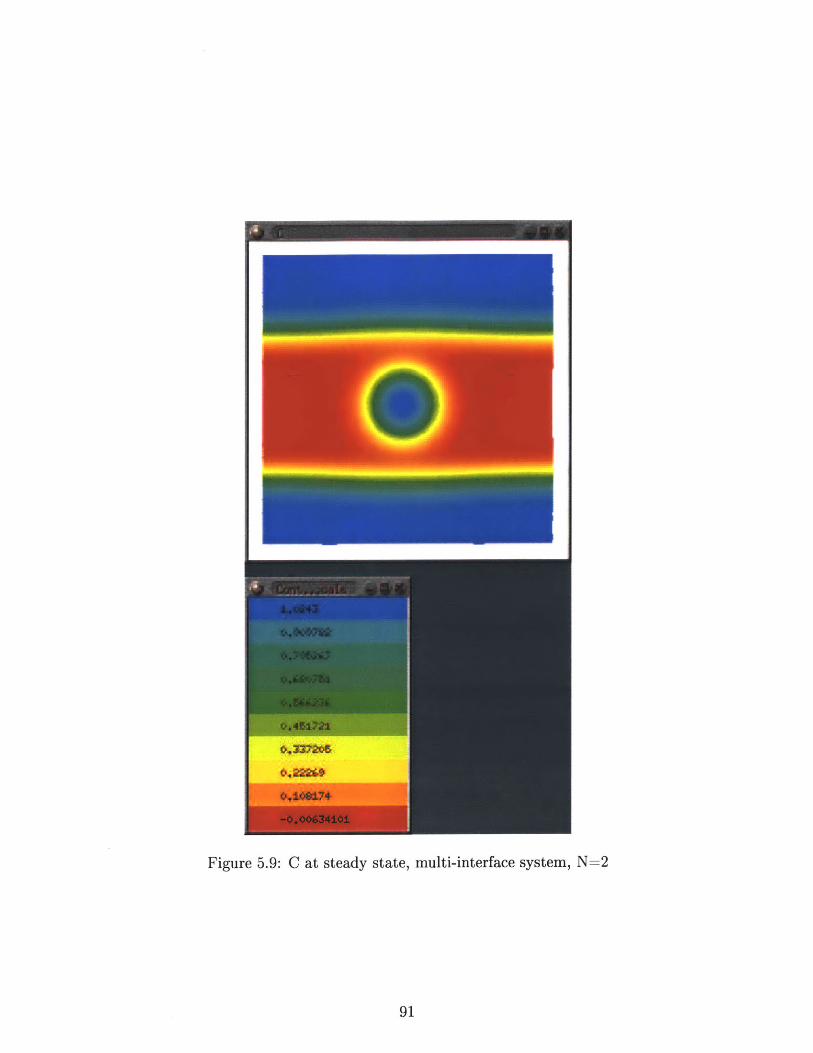
Figure 5.9: C at steady state, multi-interface system, N=2
91
.. .. ....... ...................... . ...........

Figure 5.10: C at steady state, multi-interface system, N=3
92

equation, interface motion would induce bulk fluid motion. The purpose of this section is to
simulate interface motion due to an electric field. Therefore, to simplify the equations, the
system has uniform density P = PFe, and surface tension forces are not considered. Thus, there
is no fluid velocity and the equations of motion do not need to be solved.
The governing equations are conservation of chemical species
- (pC) = MFe [KFeIlFe] + F Fe (56)atWFe FAWFe ZFe (C)
and conservation of charge
0 = * (Jeii (C) V#) (5.7)
Symmetry boundary are used for C. For voltage,
(= 0, symmetry (5.8)
x= Lx, symmetry (5.9)
05(y = 0) = 0 (5.10)
(y = LY) = 1volt (5.11)
One constraint associated with this formulation is that if FeO exists at a fixed voltage boundary,
then there will be a non-zero species flux at the boundary. The migration flux term is proportional
to aFe (C) V0. At a symmetry voltage boundary, ( t) = 0. However at a fixed voltage
boundary (5) . ii $ 0. In Fe, cFe (C) = 0, but in FeO, cFe (C) $ 0. Therefore, to conserve
species, boundaries with fixed voltage need to coincide with Fe.
The initial conditions for the first simulation are shown in Figure 5.11. There are three layers
in the y-direction, Fe(1/4cm)-FeO(1/2cm)-Fe(1/4cm). The domain is 1cm by 1cm. The grid
93

Figure 5.11: C at t=O, applied voltage
94
k zz - . .......... - - - - - I "I'll" - -a.

is 32x32, and c = dx = dy. Polynomial interpolation was used for oe (C).
Oe (C) = Oe,slag + 3 (ce,metal - Ue,s ag) C 2 - 2 (Ue,metal - Oe,siag) C 3 (5.12)
where Oe,s ag = 0 1 . The electrical conductivity of Fe in the physical system is 7 * 1051.
However for numerical stability, Ue,metaj was set to Oe,metal = 10 3 m. Recall that UFe,slag
12 s 0e,metaL UFe,slag is still satisfied. r, was scaled by 100 so that the timescale of
diffusion is less than that of migration. The rv scaling was necessary to maintain a stable interface.
A positive voltage at y = L, creates an electric field in the negative y-direction. In the FeO,
the electric field forces the Fe2 + downward and the 02- upward. Because the electrochemical
reactions at the interface are modeled as transport limited, the migration flux of species to the
interface leads directly to interface motion. Results for t = 1300s are shown in Figures 5.12 and
5.13.
The FeO phase moved a distance in the y-direction of approximately 1/8cm. Because
Oe,metal >> cFe,slag, there are very small gradients of # in Fe.
Is this result reasonable? Here a more quantitative explanation is given. The interface velocity
is given by equation 2.18.
vg - J-1currentVlag _ Jcurrent Msag (5.13)int = 2F 2F Pstag J
The flux of charge in the slag is given by
Jcurrent = -Fe d- (5.14)ZFe dy
Recall,
ZZFe - 2)- - (-2) =9 (5.15)Mo (16
95

Figure 5.12: C at t=1300s, applied voltage
96

Figure 5.13: Voltage at t=1300s, applied voltage
97
...... ......... ................................ ... .............. ....... .... ..

so (adjusting for constant density)
Jcurrent = - (12 * 2 1 1V = 2.16 A (5.16)2k. * m 0.5cm cm2
Combining gives the interface velocity
(21, 600 ) (36 * k094 ) mVint = 2(6 ) (oe) = 5.76 * 10-- (5.17)
2 (96, 485-f, (70004k3
An expected time interval for an interface movement of 1/8cm is
Vint = L m-) 2000s (5.18)7 (5.76 * 10-7 )
which agrees with the numerical simulation.
The next series of simulations deal with streamer growth due to an electric field. Two cases
are considered: (1) a perturbed cathodic interface, (2) a perturbed anodic interface. The initial
conditions are shown in Figures 5.14 and 5.15.
(The plots are symmetrical with respect to x = Recall that the voltage boundary
conditions are #(y = 0) = 0V and #(y = Ly) = 1V. Therefore, the bottom face is the cathodic
interface (Figure 5.14), and the top face is the anodic interface (Figure 5.15). Results at t =
1660sec for cathodic growth and anodic growth are shown in Figures 5.16and 5.17 respectively.
It was found in section 5.2, that it is possible to predict interface merging with diffusion alone
with the diffuse interface model depending on the choice of interface thickness. Therefore, for
reference, results for the two systems at t = 1660sec are also given for pure diffusion (no electric
field). Figure 5.18 shows diffusion results for the perturbed cathodic interface, and Figure 5.19
shows results for the perturbed anodic interface.
Also for reference, Figure 5.20 shows the steady state profile for both the cathodic and anodic
perturbed cases. The steady state result for the pure diffusion case shows that there is no artificial
interface interaction due to interface scaling. The equilibrium configuration of the systems with
98

Figure 5.14: C at t=O, perturbed cathodic interface
99
mmmm mmmm , im m mm mmmm mmmm a..m , n m~un nnan --- il iinn mielmisa ili , uu nmil 1111 , u 111111i.li...............11='1

Figure 5.15: C at t=O, perturbed anodic interface
100
..................

Figure 5.16: C at t=1660s, perturbed cathodic interface
101
.......... - -

Figure 5.17: C at t=1660s, perturbed anodic interface
102
. ........... . ............ .. .................. .

Figure 5.18: C at t=1660s, perturbed cathodic interface, no applied voltage
103
. .......... .. ............ .. ............ ..

Figure 5.19: C at t=1660s, perturbed anodic interface, no applied voltage
104
m - -m - i - - . - !n - - - ..- .... ....... "... ....... ...... ........ . --V"""""'"

Figure 5.20: C at steady state, perturbed cathodic or anodic interface, no applied voltage
105
. . ......... . ... .....

zero electric field is three layers vertically with interfacial area minimized. For the perturbed
cathodic interface, the perturbation grows with an applied voltage and decays without an applied
voltage. For the perturbed anodic interface, the perturbation decays with and without an applied
voltage. Note that the rate of decay is greater with the applied voltage than without the applied
voltage.
The interface growth can be explained by looking at the migration flux of chemical species.
The flux is proportional to the electric field.
LA# 1Vj oc E oc Oc (5.19)
L LFeO
At the perturbed regions the length of FeO is smaller than in the unperturbed region.
LFeO,perturbed < LFeO,unperturbed (5.20)
So, the flux will be greater at the perturbed site.
Jperturbed > junperturbed (5.21)
For the cathodic case, the increases flux leads to a decreased FeO length, and a growth instability
occurs leading to the formation of streamers. For the anodic case, the increased flux leads to a
decreased FeO length, and the interface stabilizes.
5.4 Diffusion, Surface Tension Driven Convection
Jacqmin [9] simulated a 2D oscillating drop with the phase field method. The calculations
were performed using four grids: 16x16, 32x32, 64x64, 128x128; and the calculated frequencies
were shown to approach the analytical result with increasing grid density. The simulation was
repeated in this project to validate the surface tension forces in the diffuse interface model. The
106

drop simulation for this project is described below.
Initially the drop is a square 1cm by 1cm. Due to symmetry, one quarter of the drop was
simulated. The drop is surrounded by a fluid of different phase. C = 1 for the drop, and C = 0
for the surrounding fluid. The drop and surrounding fluid have the same properties.
p = 1000 k (5.22)
7 = 4* 10_4 kg (5.23)m * s
N7interface = 0.03 (5.24)m
The analytical frequency is f = 47.89Hz. The governing equations are: conservation of x-
momentum
(pu) + V 0 (pru) - -p +V.e (nu)+pgx (5.25)
+ a ax
conservation of y-momentum
a(pV)+V*(p~) - + ±P Q (7jv) + pgy (5.26)
Dy Dy
conservation of mass (incompressible)
VOV=o 0(5.27)
and the phase field equation
DC (5.28)
Dt
107

which is a simplified form of equation 3.67. The solution domain is !cm by 1cm. A uniform
grid of 16x16 nodes was used (or 17x17 including extra velocity nodes). To maintain a stable
interface, , was set such that the timescale of interface diffusion is less than that of bulk fluid
motion. The phase field parameters used were
6 = Ax (5.29)
a = (v1) -y (5.30)
(v=18-) (5.31)
K = f2 (5.32)
where Ax = Ay is the grid spacing. The initial conditions for the simulation are shown in Figure
5.21. The interface is initially sharp and varies from zero to one over a single grid spacing.
The drop radius position at an angle of 45deg to the x axis was calculated by interpolating
C = 0.5. The time evolution of the radius position is shown in Figure 5.22. From the plot,
the frequency is approximately 40Hz. The frequency for 16x16 grid of Jacqmin was 40.82Hz (,
and for the128x128 grid was 44.98 Hz). Therefore, the code accurately predicts surface tension
driven flow. The system at steady state is shown in Figure 5.23. At steady state, the drop is
at equilibrium position, Req = 3cm, and the interface is smoothed out over about four grid
points.
The oscillating 2D drop simulation was repeated for an Fe drop surrounded by FeO. All
conditions are the same except for properties (see Appendix 8.1 for properties of Fe-FeO system)
. The density and viscosity of Fe and FeO each differ by a factor of two. However, the system is
still incompressible for the sharp interface formulation and is modeled as incompressible for the
diffuse interface formulation. The initial conditions and the steady state profile are exactly the
same as the case above. The time evolution of the radius position is shown in Figure 5.24. From
the plot, the frequency is approximately 80Hz. The increase in frequency is due to the increase
108

Figure 5.21: C at t=O, 2D drop
109
. . .... ..........

0.~2
*OW~
0 0.0W Q.02 0. W.0 0.05 D. 0 0.07 0.09 OAS
Figure 5.22: Radius (m) A45deg vs time (sec)
in surface tension.
5.5 Diffusion, Gravity and Surface Tension Driven Convec-
tion
The Fe drop simulation of the previous section is extended here to include a gravitational field
= -9.811. The initial conditions are the same (Figure 5.21). Steady state results are shown
in Figure 5.25. Comparing this result to that of g = 0 (Figure 5.23), the drop under gravity is
slightly compressed in the y-direction. The radial positions at 90deg from the x-axis is denoted
as h. For the zero g case,
h = 5.53mm (5.33)
and for the nonzero g case,
h= 5.08mm (5.34)
The compression due to gravity is balanced by surface tension forces. Note that because of the
symmetry boundary condition at y = 0, the drop has a wetting angle of 90deg.
The equilibrium configuration of the system can be explained with thermodynamics. Let the
110

0', WW6
Figure 5.23: C at steady state, 2D drop
111
... ... ..... ...... ......... .... .. ................. ...............

.OW2
OOA2
0 0.% 0.01 -MIS1 0.02 0.02 0.03
Figure 5.24: ,Radius (m) 445deg vs time (sec)
initial conditions be state 1 and equilibrium be state 2. The system is modeled as an isolated
incompressible system (zero flux boundary conditions) undergoing an irreversible run down to
equilibrium. The first law reads
Q-W= AU+APE+AKE (5.35)
which simplifies to
0 = AU + APE (5.36)
Using constitutive relations,
0 = mc, (T2 - Ti) + mg (y2 - j+1 ) +y (A2 - A,) (5.37)
where V is the center of gravity of the system and A is the surface area of the interface. The
final configuration can be found by a force balance at the interface. The first law gives the final
temperature of the system. The second law reads
AS = Sin - Sout + Sgen (5.38)
112
-- ---------- - -- -..... ......... - ==N

Figure 5.25: C at steady state, 2D drop with gravity
113

Since the system is thermally insulated, there is no entropy transfer.
AS = Sgen (5.39)
Using constitutive relations,
mcIn ( = Sgen (5.40)T1
The second law gives the entropy generated during the process. The equilibrium state is charac-
terized by a maximum entropy. Looking at the entropy change for the system,
AS = mc, ln (T) (5.41)T,
Using the first law,
AS=mc ln 1- mg/y +yA) (5.42)mcT1
To maximize AS is to minimize APE under the constraint of conservation of mass. At state 2,
(PE)2 = mgy2 + yA 2 (5.43)
If g = 0, then to maximize entropy A2 is minimized forming a circle. If 7 = 0, then to maximize
entropy Y2 is minimized forming a horizontal interface with Fe on the bottom. For intermediate
cases where g 0 0 and -y : 0, there is an optimum balance between the two terms leading to the
compressed configuration.
An analytical result for the drop height h(x = 0) is obtained by an overall force balance in
the x-direction
w = (pi. (y) - pat (y)) wdy (5.44)
where w is the z-direction width. The pressure inside the drop is related to the pressure outside
114

the drop by the surface tension and radius of curvature R. The pressures can be written,
Pout (y) = pt (y = h) + poutg (h - y)
Pin (y) = pt (y = h) + + Ping (h - y)|Rhj
where Rh = R (x = 0, y = h). Substituting for pressure,
h+ (pin - pout) g|Rh |
(h - y)) dy
which simplifies to
(5.48)
Note that when h = IRh 1, Apg = 0. Therefore, for a circular profile, either /p = 0 or g = 0.
Introducing the equilibrium drop radius for g = 0, Req, and rearranging gives,
ApgReq
2-y h q 2
Req+Req h+ Rh 1 = 0|Rh| Req
(5.49)
which is solved with the quadratic equation. For this simulation, Req = 5.53mm, h (i = 0) =
5.079mm, h (i = 1) = 5.052mm. The radius of curvature is approximated by
- 2h (i = 0)(,AX)2
+ h (i = 1))
using a shadow node. Using this radius of curvature, the force balance gives
) = 0.876
The measured value ish (i = 0)
Req
_5.079- = 0.9185.53
115
(5.45)
(5.46)
(5.47)
(5.50)
(hanalyticai
Req(5.51)
(5.52)
y=hY=0 h
7 = -h+ Apg- |Rh| 2
1 d 2h (h (i = 1)Rh dX2

which gives an error of approximately 5%. Therefore, the model accurately captures the balance
between surface tension forces and gravitational forces.
116

Chapter 6
Discussion
6.1 Introductory Remarks
In this chapter, important assumptions used in the model formulation are revisited, other appli-
cations for the model are introduced, and reasons and suggestions for future development of the
model are given.
6.2 Assumptions and Limitations
The electrochemical reactions in the model are limited to the transport limited regime. This
assumption is valid for electrolysis systems similar to the one described in this thesis. In high
temperature systems such as the one discussed here, the mass transfer resistance is much greater
than the charge transfer resistance. However, the transport limited regime also corresponds to
a zero cation concentration at the cathodic interface. If the full electrochemical current-voltage
equations were used, then there would be an exponential response to any significant concentration
at the interface, but since the constitutive current-voltage relations are explicitly limited to the
transport limited case, the reaction behaves as if the concentration is zero at the interface.
Thy physical slag/metal system is a multi-component system and has a concentration bound-
ary layer. The binary system does not have a concentration boundary layer. Additional cations
117

are needed to maintain charge neutrality in a concentration boundary layer. One way to capture
a diffusion boundary layer would be to extend the formulation to ternary systems. Since there
is no boundary layer in the binary system, there is no diffusion resistance associated with the
interface motion. Thus with less resistance, the model predicts a larger reaction rate for a given
applied voltage than would be expected. However, the model does capture important electrode
phenomena such as interface motion and perturbation growth and decay.
The free energy curve was modeled with a polynomial function, and the interface thickness was
scaled to a mesoscopic length. Both approximations serve to change the diffusion characteristics
of the system. The diffusion flux is proportional the gradient in chemical potential which is a
function of the free energy curve. The polynomial approximation captures the interfacial energy
of the system, but the exact level of curvature is lost. For example, a large (absolute value of)
second derivative of the homogeneous free energy, T", at C = 0 or C = 1 corresponds to a large
change in free energy for concentrations that stray from equilibrium. Conversely, a small second
derivative corresponds to a small free energy change. Since, the driving force for diffusion is a
reduction in free energy, each case leads to a different diffusion flux. In the phase field model,
a is scaled by E and 0 is scaled by 1/c. Therefore, interface scaling artificially increases a and
lowers #. Lowering # lowers the peak in the free energy curve. The implications are a lower "
near equilibrium concentrations and a lower activation barrier for interface diffusion. a is the
gradient penalty coefficient in the free energy equation and acts as a driving force for interfacial
gradient minimization. An artificially large a increases this driving force. The surface tension is
proportional to \ , so it is unaffected by the scaling. Thus, interface scaling leads to a number
of issues involving diffusion for systems away from equilibrium, but the model does capture the
macroscopic surface tension.
Assuming rapid charge redistribution throughout the system, the conservation of charge equa-
tion reduced to an equation for zero divergence of charge flux due to migration. Mathematically
speaking, the charge equation reduced to an equation with a single unknown, voltage, signifi-
cantly reducing the coupling of the equations. The unsteady and convection terms were safely
118

neglected even in systems with forced convection. However, the diffusion term was not so safely
neglected with respect to the migration term. Recall that the representative dimensionless num-
ber was on the order of N2 - 10-2 (equation 3.87). For the Fe-FeO system analyzed here, this
was a conservative estimate but may break down for other systems such as multi-component
or aqueous solutions. The concentration difference used was conservative for the binary Cahn-
Hilliard system where the mole fraction varied from 1/2 to 1. Other systems may exhibit larger
concentration differences which would raise the dimensionless parameter by a factor of 10 or so.
Also, the conductivity of slag was used instead of the conductivity of steel. For the binary sys-
tem, concentration differences characterize the diffuse interface and so coincide with all property
differences including conductivity. If the conductivity of steel was used, then N2 would have
decreased by a factor of 1000.
The system modeled was considered to be isothermal. Chemical reactions serve as heat sinks
and sources. Also, electrical current and high resistance levels lead to joule heating which is
another heat source. The question is whether local variations in temperature have a significant
effect on the transport of chemical species. Conservation of energy governs the temperature
distribution throughout the system. Transport properties typically have a strong dependence on
temperature. The mass and specific heat capacity of the system serve as estimate to the sensi-
tivity of temperature to heat flux, and the heat conductivity serves as a measure of temperature
gradients. Another important factor is heat transfer boundary conditions. If the temperature of
the surroundings are much lower than the solution, then large temperature differences may exist
in the solution. In applying this model to real systems, scaling analysis similar to that in this
thesis should be done to ensure that the isothermal approximation is valid.
6.3 Applications
The model developed here would also serve as a useful tool for analyzing existing processes such
as magnesium reduction and aluminum reduction. Both are two phase liquid/liquid systems
119

with transport limited electrochemical reactions. An important feature in the steel refining
system is the presence of streamers which complicate cathode dynamics considerably. The model
predicts the growth of streamers and could be used in the development of efficient cathode
designs. Improving efficiency of refining systems not only improves production but also, just as
importantly, significantly reduces the amount of waste.
One system where hazardous waste is particularly problematic is titanium reduction. Current
practice involves the use of chlorime gas as apposed to an electrolytic solution. In titanium
reduction, ionized titanium exists as Ti 2+, Ti 3 +, and Ti4 +. There is a higher thermodynamic
driving force for Ti4+ to reduce first. The Ti2+ and TiO+ build up near the cathode and diffuse
away toward the anode and give up electrons and form TiO+ and Ti4 +. Then, the Ti4 + migrates
to the cathode, and the circular pattern continues hindering production rates. (It is worth noting
that attemps to reduce hexavalent chromium electrolytically have exhibited the same inefficient
circular patterns.) A new method currently being researched at Boston University for avoiding
the titanium reoxidation problem is through the use of an anode which is an ionic conductor. The
anode is coated with a material that has a high oxide ion diffusivity, a low electron conductivity,
and a low titanium diffusivity. Therefore, only the oxide ions are allowed to pass through and be
oxidized. The model developed here could be used in developing these new systems which would
serve to answer current economic and environmental issues.
6.4 Future Work
The simplified 2D Fe-FeO-Fe system does not capture all phenomena of the physical slag-metal
system, but does provide a foundation for a more comprehensive model to be developed in
the future. The Cahn-Hilliard model restricts the fluid to two components, eliminating multi-
component interactions. The capillary instability is a 3-D phenomenon and does not exist in a
2-D system. For these reasons, a 3-D, multi-component system will need to be developed in future
work in order to accurately predict the relationship between design parameters and reaction rate
120

of the chosen application. However, the the extension of the code to 3-D is straightforward and
is a matter of computer storage and speed.
Other more fundamental advances to the model include electrocapillarity, multiphase liq-
uid/solid/gas interactions, magnetic effects, and thermal effects. Electrocapillarity, the variation
of surface tension with electric field, affects all interface surface tension related phenomena such
as streamer growth, oscillation, and breakup. To include the solid electrode in the computer
simulation would be very beneficial to electrode design. Also, many systems like the titanium
system described above involve the reduction of a solid metal from a liquid electrolyte, and
require fluid/structure (or liquid/solid) interactions for modeling. The oxidation of oxygen in
slag systems produces gases such as CO, 02, H 20, etc. These gases enhance mass transfer by
convection and thus enhance reaction rate. An idea which has not yet been investigated through
experimention on electrolytic refining systems is the application of magnetic fields. The gen-
eral Lorentz force law reads P = q(? + V x -9), where 74 is the magnetic field vector, q is
charge, and V is the velocity of charge. Intelligent application of magnetic fields may potentially
enhance overall process control. Finally, for systems with relatively low heat capacities and ther-
mal conductivities, the energy equation would allow for more accurate representation of system
properties by providing the local temperature.
The finite element method may compliment future developments. Unstructured grids would
provide the flexibility needed to increase grid density at a curved interface. Also, Lagrangian
descriptions may be used in the development of solid/liquid/gas interactions which would require
different meshing schemes in each phase.
121

Chapter 7
Conclusions
In this thesis, a diffuse interface model for a two component liquid/liquid, isothermal system
undergoing transport limited electrochemical reactions was developed. The model was applied
to the electric field enhanced smelting and refining of steel process. A representative Fe-FeO
system was used as a simplified model. The governing equations were derived for the most
general case first. Then, using a series of asymptotic solutions, length, velocity, and time scales
were derived. Based on the simple scaling arguments, the governing equations were significantly
simplified. In particular, the conservation of charge equation, which governs the voltage field,
was reduced from an equation involving concentration, velocity, and voltage with time and space
derivatives to an equation involving just voltage with a spatial derivative.
The system of equations were discretized using the finite-difference method and the Crank-
Nicholson scheme. Symmetry boundary conditions were used for concentration and were im-
plemented with shadow nodes. The system of nonlinear difference equations were solved using
the matrix-free Newton-Krylov method. PETSc was used for distributed array data storage and
parallel processing.
A series of case study simulations involving the electrochemical Fe-FeO system were used to
display phenomena characteristic of refining systems. The case studies showed that the model
accurately predicts:
122

. Inter-phase diffusion
" Interface motion due to an electric field
* Growth of cathodic interface perturbations into streamers due to an electric field
" Decay of anodic interface perturbations due to a voltage field
* Interface oscillations due to surface tension driven flow
" Interface distortion due external body forces
The simplified 2D Fe-FeO-Fe system does not capture all phenomena of the physical slag-metal
system, but does provide a foundation for a more comprehensive model to be developed in the
future. The model developed here is general in the sense that it can be used to model any
application with similar physical interactions, and the methodology developed here for coupling
transport limited electrochemistry with transport equations is fundamental in that the extension
to more complex systems is limited only by the development of a free energy model and system
properties.
123

Chapter 8
Appendix
8.1 Properties
DFe2+ 10 -Ferrous ion diffusivity in slagS
Ny ~ 1-Fe - FeO interfacial energy
mkg
Pmeta = 7160-density of metal
pag Pmeta density of slag
k grqmetal = 0.006 viscosity of metal
m * s
77siag = 2 7metalviscosity of slag
51O-e,metal 7.14 * 105 electrical conductivity of Fe
Q * M
8.2 Computer Program
The computer program used for this project can be found at lyre.mit.edu/~dussault.
124

Bibliography
[1] Allen J. Bard and Larry R. Faulkner, Electrochemical Methods, John Wiley & Sons,
New York ,1980.
[21 R. Byron Bird, Warren E. Stewart, and Edwin N. Lightfoot, Transport Phenomena,
John Wiley & Sons, New York, 1960.
[3] David J. Griffiths, Introduction to Electrodynamics, Second Edition, Prentice Hall, Upper
Saddle River, New Jersey 07485, 1989.
[4] W.W. Mullins and R.F. Sekerka, Morphological Stability of Particle Growing by Diffu-
sion or Heat Flow, Journal of Applied Physics, Vol. 34, No. 2, pp. 323-329, Feb. 1963.
[5] W.W. Mullins and R.F. Sekerkam, Stability of a Planar Interface During Solidification
of a Dilute Binary Alloy, Journal of Applied Physics, Vol. 35, No. 2, pp. 444-451, Feb. 1964.
[6] Suhas V. Patankar, Numerical Heat Transfer and Fluid Flow, Washington, Hemisphere
Pub. Corp., New York, McGraw-Hill, 1980.
[71 Lloyd N. Trefethen and David Bau III, Numerical Linear Algebra, Society for Industrial
and Applied Mathematics, Philadelphia, 1997.
[8] Francis B. Hildebrand, Advanced Calculus for Applications, Second Edition, Prentice-
Hall, Inc., Englewood Cliffs, New Jersey, 1976.
125

[9] David Jacqmin, Some Convergence Results for Phase-Field
Surface Tension Modeling of Two-Phase Navier-Stokes Flow,
The 1997 ASME Fluids Engineering Divisions Summer Meeting, June 22-26, 1997.
[10] David Jacqmin, An Energy Approach to the Continuum Surface Tension
Method: Application to Droplet Coalescences and Droplet/Wall Interactions,
Proceedings of the ASME Fluids Engineering Division, FED-Vol. 234, 1995 IMECE,
ASME 1995.
[11] N. Saunders and A.P. Miodownik, CALPHAD, Calculation of Phase Diagrams, A
Comprehensive Guide, Pergamon, 1998.
[12] E.T. Turkdogan, Fundamentals of Steelmaking, Institute of Materials, London, 1996.
[13] U.B. Pal, S.A. MacDonald, D.W. Woolley, A.C. Powell and C.P. Manning, En-
hancing Electrochemical Reactions in Smelting and Refining Operations, 2001 Electric Fur-
nace Conference Proceedings, ISS publication, pp. 323-336, 2001.
[14] D.M. Anderson and G.B. McFadden, A Diffuse-Interface Description of Fluid Systems,
Applied and Computational Mathematics Division, National Institute of Standards and
Technology, Gaithersburg, MD, Report No. NISTER 5887, August 1996.
[15] J.E. Hilliard, Spinoidal Decomposition, pages 497-560, American Society for Metals Press,
Metals Park, Ohio, 1970.
[16] J. J. Hoyt, The Continuum Theory of Nucleation in Multicomponent Systems,
Acta Metall. Mater. ,Vol. 38, No. 8, pp. 1405-1412, 1990.
[17] Zhiqiang Bi, Robert F. Sekerka, Phase-field model of solidification of a binary alloy,
Physica A, pp. 95-106, 1998.
126

[181 J.A. Warren and W.J. Boettinger, Prediction of Dendritic Growth and Microsegregation
Patterns in a Binary Alloy Using the Phase-Field Method, Acta metall. mater.,Vol. 43, No.
2, pp. 689-703, 1995.
[191 David Jasnow and Jorge Vinals, Coarse-Grained Description of Thermo-Capillary Flow,
Phys. Fluids 8 (3), pp. 660-669, March 1996.
[20] R. Tonhardt and G. Amberg, Phase-Field Simulation of Dendritic Growth in Shear
Flow, Journal of Crystal Growth 194, pp. 406-425, 1998.
[21] Ravi Chella and Jorge Vinals, Mixing of Two-Phase Fluid by Cavity Flow,
Physical Review E, Vol. 53, No. 4, pp. 3832-3840, April 1996.
[22] MIT class notes, class title: Kinetic Processes in Materials, class number: 3.21, Spring 2001.
[23] MIT class notes, class title: Introduction to Numerical Simulation, class number: 2.096, Fall
2001.
[24] MIT class notes, class title: Numerical Methods for Partial Differential Equations, class
number: 2.097, Spring 2001.
127