A DESIGN-BASED APPROACH TO K-NN TECHNIQUE IN FOREST INVENTORIES 27 Marzo 2008 GRASPA Conference 2008...
94
A DESIGN-BASED APPROACH TO K-NN TECHNIQUE IN FOREST INVENTORIES 27 Marzo 2008 GRASPA Conference 2008 F. Baffetta, L. Fattorini and S. Franceschi
-
Upload
clarissa-whitehead -
Category
Documents
-
view
216 -
download
0
Transcript of A DESIGN-BASED APPROACH TO K-NN TECHNIQUE IN FOREST INVENTORIES 27 Marzo 2008 GRASPA Conference 2008...

A DESIGN-BASED APPROACH TO K-NN TECHNIQUE IN
FOREST INVENTORIES
27 Marzo 2008
GRASPA Conference 2008
F. Baffetta, L. Fattorini and S. Franceschi

INTRODUCTION
Several techniques for assessing natural resources employ information from remotely sensed imagery and ground data.

INTRODUCTION
Between these methodologies, the k-Nearest Neighbours (KNN)
technique is becoming increasingly popular

INTRODUCTION
Main application: forest attribute mapping
Data: auxiliary variables for all population units (the digital numbers from multispectral
remotely sensed imagery )
interest variable values for sampled units
Between these methodologies, the k-Nearest Neighbours (KNN)
technique is becoming increasingly popular
OBJECTIVE
The statistical properties of the k-NN method are still not clearly delineated.
The only advanced investigations lie in a complete model-based setting (Kim and Tomppo (2006) and McRoberts et al. (2007) )
OBJECTIVE
The statistical properties of the k-NN method are still not clearly delineated.
The only advanced investigations lie in a complete model-based setting (Kim and Tomppo (2006) and McRoberts et al. (2007) )
•Assumptions on superpopulation models frequently unrealistic
•Neglect the fact that data arise from a pre-determined scheme of sampling

THE GOAL:
Derive the statistical properties of the k-NN estimators in a completely design-based framework
no assumption about populations
OBJECTIVE
The statistical properties of the k-NN method are still not clearly delineated.
The only advanced investigations lie in a complete model-based setting (Kim and Tomppo (2006) and McRoberts et al. (2007) )
•Assumptions on superpopulation models frequently unrealistic
•Neglect the fact that data arise from a pre-determined scheme of sampling

Study region
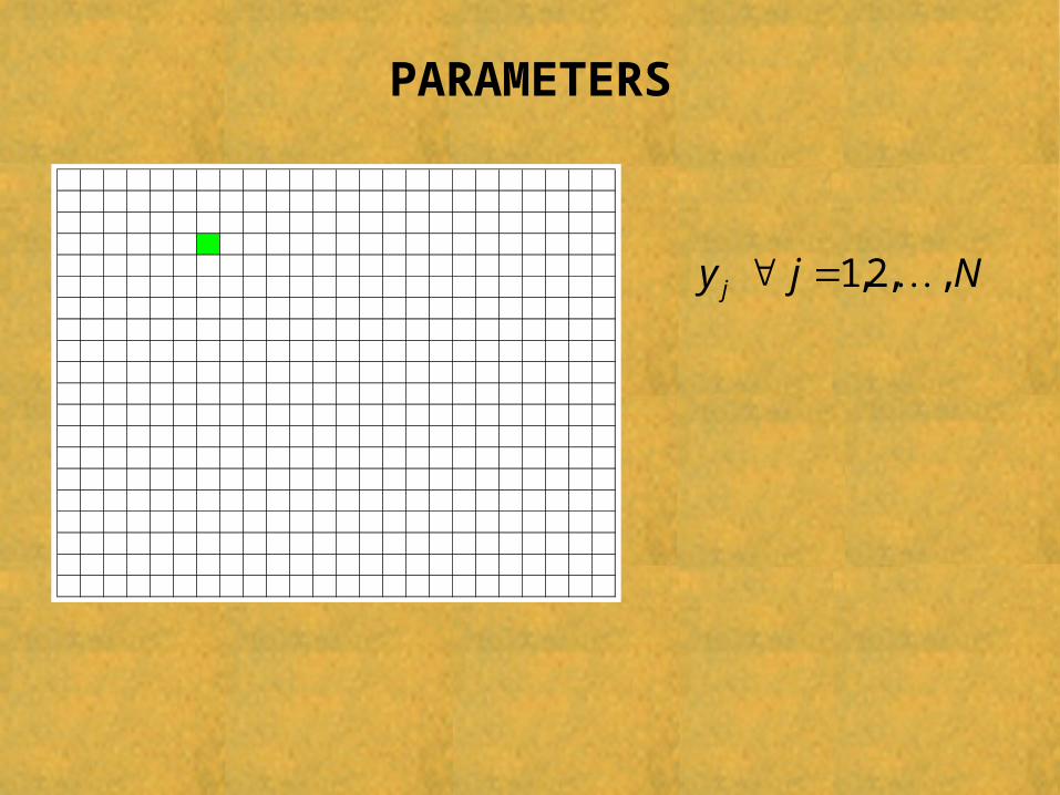
POPULATION

Study region
POPULATION
usually a set of pixels
constituting a digital image
N,...,2,1U

Study region
POPULATION
usually a set of pixels
constituting a digital image
N,...,2,1U
Y the interest variable
Y1, Y2,..., YN population values
PARAMETERS
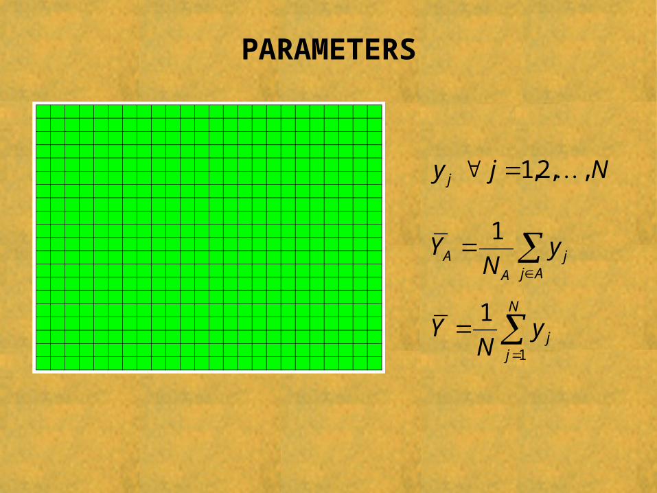
Njy j ,,2,1

PARAMETERS
Njy j ,,2,1
Aj
jA
A yN
Y1
PARAMETERS
Njy j ,,2,1
Aj
jA
A yN
Y1
N
jjy
NY
1
1

SATELLITE INFORMATION
q auxiliary variables
known for all population units
(the values of the spectral bands )
qXX ,,1
X-spaceUjjx

FOREST INVENTORY DATA
Sjp j

CONVERTING INVENTORY DATA TO PIXEL DATA
S jpy jj

CONVERTING INVENTORY DATA TO PIXEL DATA
reference set (sample)US
Sjy j
SU target set

K-NN ESTIMATION
Y
X-space
Y space
K=4
some notations
H(j,k) = label of the unit of S whose distance from unit j in U–S has rank k (k = 1,2,…,n)
unit j in U – S
units in S
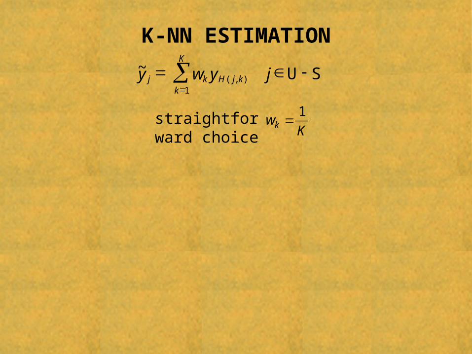
K-NN ESTIMATION
straightforward choice K
wk1
SU
jywyK
kkjHkj
1),(
~

K-NN ESTIMATION
Aj
jA
NNkA yN
Y ~1~
N
jjNNk y
NY
1
~1~
(mean estimate in the subarea of interest)
(overall mean estimate)
straightforward choice K
wk1
SU
jywyK
kkjHkj
1),(
~

K-NN ESTIMATION
BIAS? ACCURACY?
Aj
jA
NNkA yN
Y ~1~
N
jjNNk y
NY
1
~1~
(mean estimate in the subarea of interest)
(overall mean estimate)
straightforward choice K
wk1
SU
jywyK
kkjHkj
1),(
~

DESIGN-BASED INFERENCE
Design-based inference is solely determinated by the characteristic of the sampling scheme and, in contrast with model-based inference, it avoids any assumption about the
population
see Gregoire (1998) for a revision of the approaches in forestry
y1, y2, …, yN fixed
S sample of pixels selected from U by a probabilistic sampling scheme
pixels inclusion probabilitiesN ,...,, 21

DESIGN-BASED INFERENCE
h(j,r) = label of the unit whose distance from unit j has rank r (r = 1,2,…,N-1)
h(j,r) are known
X-space
Dx

DESIGN-BASED INFERENCE
unit in S
S random H(j,k) are random variables
X-space X-space
K=4

DESIGN-BASED INFERENCE
• Model-based framework UNBIASED
• Design-based framework BIASEDjy~
1
1,
~N
rrjhjrj ywyE
jrw expected weight assigned to the pixel whose distance from j has rank r in the sequence of the N-1 distances from pixel j (completely known from the sampling scheme)
can be obtained in a very similar way but it cannot be estimated on the basis of the sample data.
jyMSE ~
jy~
DESIGN-BASED ESTIMATION OF MEAN
Owing to the design-based bias induced by each the estimator may provide a highly-biased estimator for the mean over the whole study area.
jy~
NNkY
~

DESIGN-BASED ESTIMATION OF MEAN
Owing to the design-based bias induced by each the estimator may provide a highly-biased estimator for the mean over the whole study area.
jy~
NNkY
~
A more suitable estimator of turns out to beY
SU j j
jj
jjNNk
yy
Ny
NEYY
~1~1~~~
where denotes the Horvitz-Thompson (HT) estimator ofE~
UU j
jj
jj eN
yyN
E1~1

DESIGN-BASED ESTIMATION OF MEAN
Bias of closed expression
Variance of cumbersome
Y~
Y~

DESIGN-BASED ESTIMATION OF MEAN
Y~
Y~
•
• 00
2
1~~hj
j h hj
hjjhlin ee
NYVYV
U U
00jjj yye
K
kkjhkj ywy
1,
0
YYE
zyy
NYY
lin
jjj
j
jjlin
~
~1~~ 0
U
Bias of closed expression
Variance of cumbersome

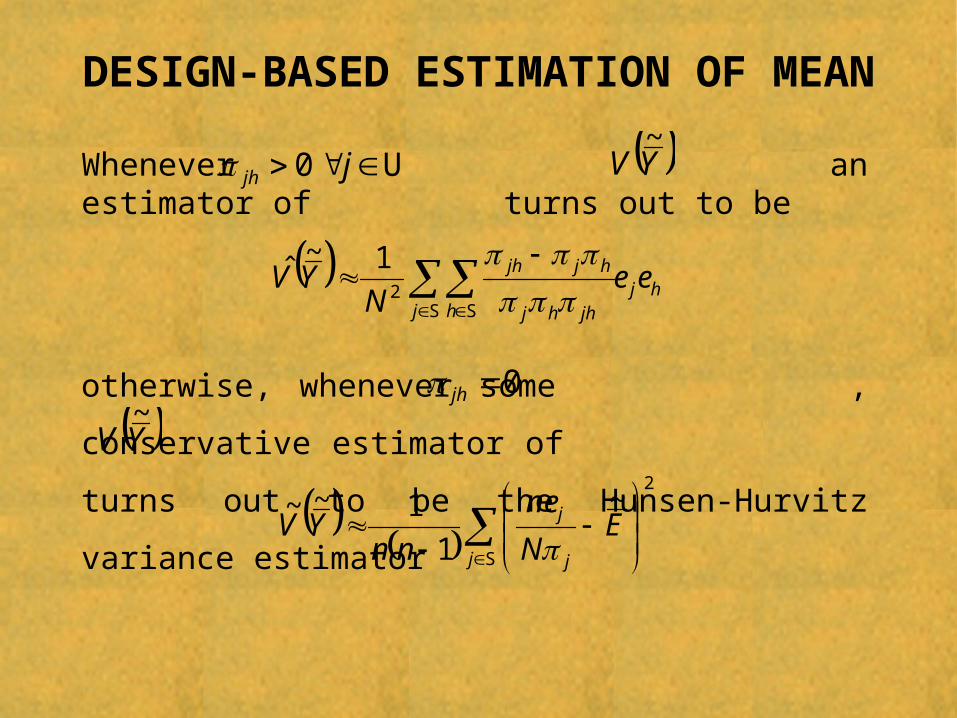
DESIGN-BASED ESTIMATION OF MEAN
Whenever an estimator of turns out to be
hjj h jhhj
hjjh eeN
YV
S S
2
1~ˆ
U jjh 0 YV~
DESIGN-BASED ESTIMATION OF MEAN
Whenever an estimator of turns out to be
hjj h jhhj
hjjh eeN
YV
S S
2
1~ˆ
U jjh 0 YV~
otherwise, whenever some , conservative estimator of
turns out to be the Hunsen-Hurvitz variance estimator
Sj j
j EN
ne
nnYV
2~
1
1~~
0jh
YV~

ASYMPTOTIC RESULTS
To the derivation of the asymptotical properties of it is necessary to think of a sequence of populations with corresponding population sizes that increase along with sample sizes
Y~
lU lN
ln
Suppose that: , , , and any l lN ln by j lj U

ASYMPTOTIC RESULTS
To the derivation of the asymptotical properties of it is necessary to think of a sequence of populations with corresponding population sizes that increase along with sample sizes
Y~
lU lN
ln
Suppose that: , , , and any l lN ln by j lj U
• sufficient conditions for asymptotic unbiasedness are given
• sufficient conditions for consistency are given

• it is proved that under SRSWOR, is asymptotically unbiased
ASYMPTOTIC RESULTS
To the derivation of the asymptotical properties of it is necessary to think of a sequence of populations with corresponding population sizes that increase along with sample sizes
Y~
lU lN
ln
Suppose that: , , , and any l lN ln by j lj U
• sufficient conditions for asymptotic unbiasedness are given
lY~
• sufficient conditions for consistency are given

ESTIMATION FOR SUB-POPULATIONS
Study region
N,...,2,1U

ESTIMATION FOR SUB-POPULATIONS
Study region
N,...,2,1U
Sub-region A
AA N,...,2,1

ESTIMATION FOR SUB-POPULATIONS
Study region
N,...,2,1U
Sub-region A
AA N,...,2,1
ASSA
• the auxiliary information is restricted to the ’s for each
• the sample information is restricted to the ’s for each
• the inclusion probabilities remain the same
jx
jy
Aj
ASj
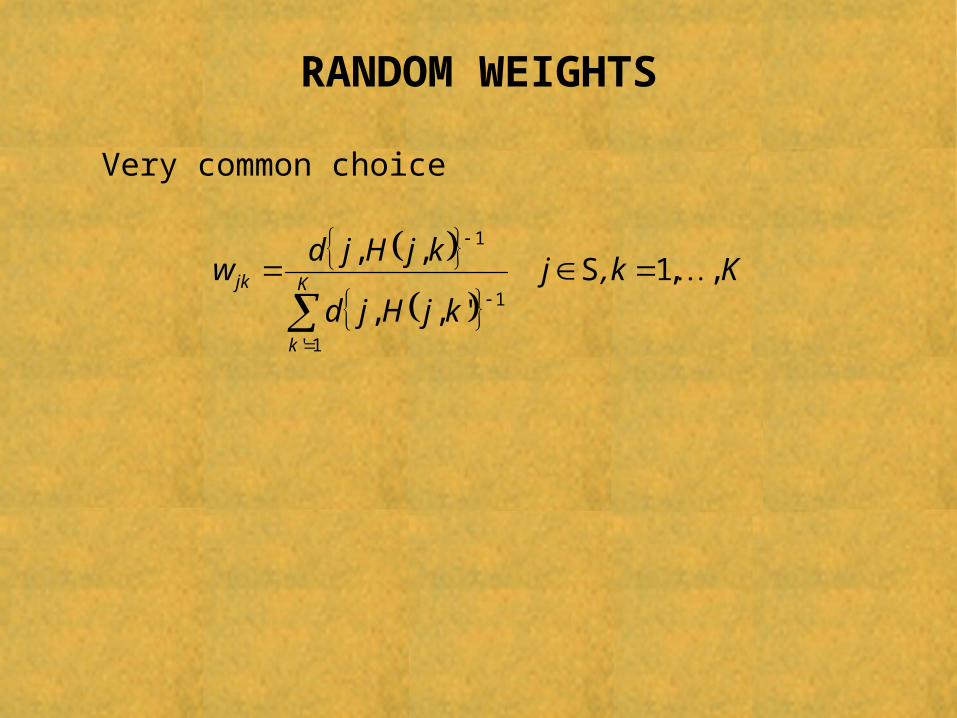
RANDOM WEIGHTS
Very common choice
Kk,jkjHjd
kjHjdw K
k
jk ,,1',,
,,
1'
1
1
S
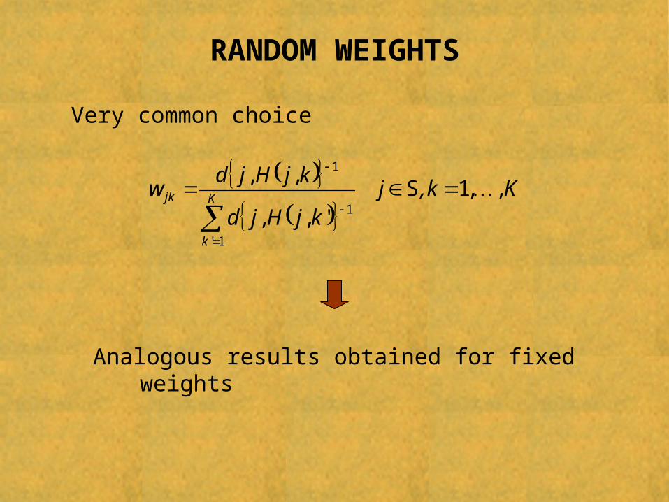
RANDOM WEIGHTS
Very common choice
Kk,jkjHjd
kjHjdw K
k
jk ,,1',,
,,
1'
1
1
S
Analogous results obtained for fixed weights

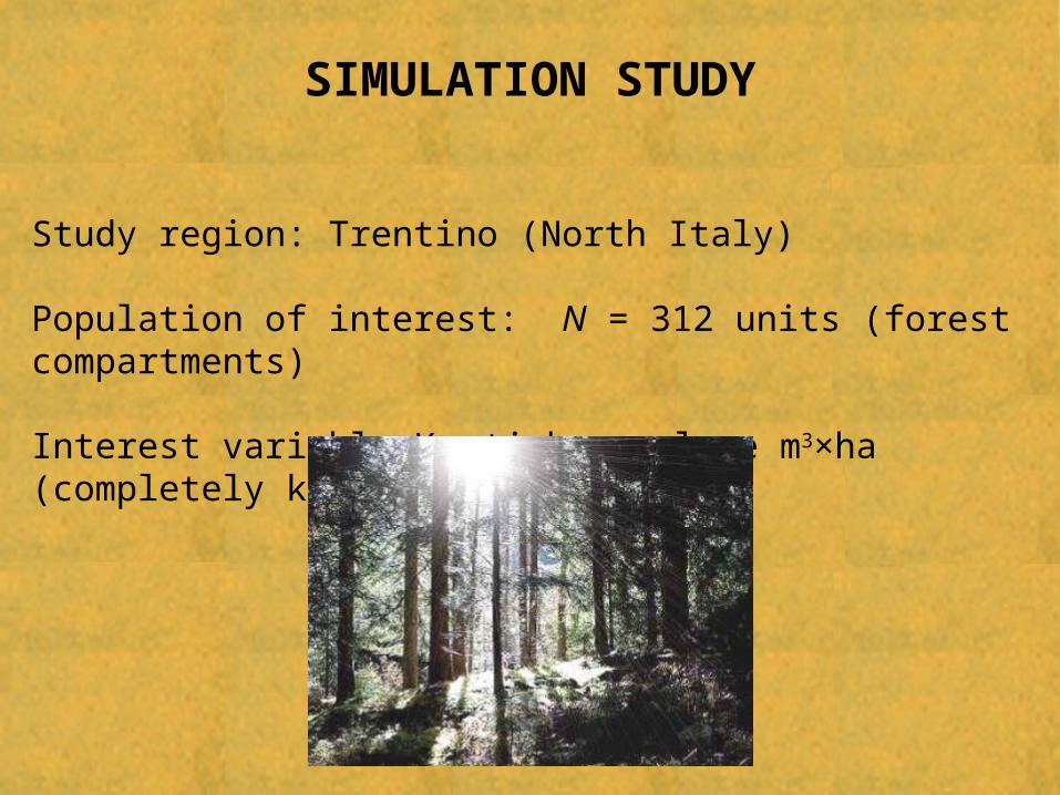
SIMULATION STUDY
Study region: Trentino (North Italy)

SIMULATION STUDY
Study region: Trentino (North Italy)
Population of interest: N = 312 units (forest compartments)
SIMULATION STUDY
Study region: Trentino (North Italy)
Population of interest: N = 312 units (forest compartments)
Interest variable Y : timber volume m3×ha (completely known)

SIMULATION STUDY
Study region: Trentino (North Italy)
Population of interest: N = 312 units (forest compartments)
Interest variable Y : timber volume m3×ha (completely known)
Auxiliary variables: 6 spectral bands (obtained from the optimal bands of ETM+ acquisitions)
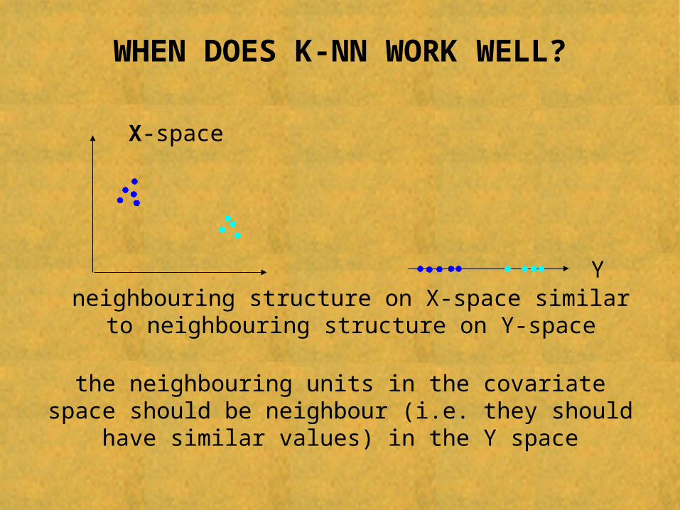
WHEN DOES K-NN WORK WELL?
Y
X-space
neighbouring structure on X-space similar to neighbouring structure on Y-space
the neighbouring units in the covariate space should be neighbour (i.e. they should have similar values) in the Y space

MULTIDIMENSIONAL SCALING (MDS)
X-space
Z0
MDS Dx = Dz

MULTIDIMENSIONAL SCALING (MDS)
NjzSYy jYj ,...,2,1,
X-space
Z0
MDS
YY
YS YSDY = const DZ
Dx = Dz

MULTIDIMENSIONAL SCALING
0
100
200
300
400
500
600
700
800
-40 -20 0 20 40 60Z
ZSY Y
This should be the best situation for K-NN
12 YZR

MULTIDIMENSIONAL SCALING
jjYj ezSYy
Perturbing this situation should deteriorate
the performance of K-NN
0
100
200
300
400
500
600
700
800
-40 -20 0 20 40 60Z
ZSY Y
This should be the best situation for K-NN
12 YZR

0
100
200
300
400
500
600
700
800
-40 -20 0 20 40 60
PSEUDO-POPULATIONS
eSZY
Z
8.02 YZR

0
100
200
300
400
500
600
700
800
-40 -20 0 20 40 60
PSEUDO-POPULATIONS
eSZY
Z
6.02 YZR

0
100
200
300
400
500
600
700
800
-40 -20 0 20 40 60
PSEUDO-POPULATIONS
eSZY
Z
4.02 YZR

0
100
200
300
400
500
600
700
800
-40 -20 0 20 40 60
PSEUDO-POPULATIONS
eSZY
Z
2.02 YZR

0
100
200
300
400
500
600
700
800
-40 -20 0 20 40 60
REAL POPULATION
Z
Y
3.02 YZR

MONTE CARLO EXPERIMENT
10,000 simulations
Sampling scheme adopted: SRSWORN =312, n = 16 (5%), 31 (10%), 62 (20%), 94 (30%)
K = 1,2,,…,12

MONTE CARLO EXPERIMENT
10,000 simulations
Sampling scheme adopted: SRSWORN =312, n = 16 (5%), 31 (10%), 62 (20%), 94 (30%)
K = 1,2,,…,12
YRB~
YRME~
YVRB~~

SIMULATION RESULTS YRME~
0%
1%
2%
3%
4%
5%
6%
7%
8%
9%
10%
1 2 3 4 5 6 7 8 9 10 11 12
0%
1%
2%
3%
4%
5%
1 2 3 4 5 6 7 8 9 10 11 12
94n
3.02 YZR2.02 YZR 4.02 YZR 6.02 YZR 8.02 YZR 12 YZR
K
0%
2%
4%
6%
8%
10%
12%
14%
1 2 3 4 5 6 7 8 9 10 11 12
16n
K
31n
K
0%
1%
2%
3%
4%
5%
6%
7%
1 2 3 4 5 6 7 8 9 10 11 12
62n
K

SIMULATION RESULTS YVRB~~
3.02 YZR2.02 YZR 4.02 YZR 6.02 YZR 8.02 YZR 12 YZR
-21%
-16%
-11%
-6%
-1%
4%
9%
14%
19%
24%
1 2 3 4 5 6 7 8 9 10 11 12
-21%
-16%
-11%
-6%
-1%
4%
9%
14%
19%
24%
1 2 3 4 5 6 7 8 9 10 11 12
16n
-21%
-16%
-11%
-6%
-1%
4%
9%
14%
19%
24%
1 2 3 4 5 6 7 8 9 10 11 12
-21%
-16%
-11%
-6%
-1%
4%
9%
14%
19%
24%
1 2 3 4 5 6 7 8 9 10 11 12
62n
K
K
K
K
94n
31n

To compare k-NN with an alternative common way to handle auxiliary information
Generalized Regression Estimator (GREG)
(model assisted)
bxX ˆˆ TGREG yY
Sj
jyn
y1
Uj
jNxX
1
Sj
jnxx
1
SS jjj
j
Tjj y xxxb
1
ˆ
K-NN AND GREG

To compare k-NN with an alternative common way to handle auxiliary information
Generalized Regression Estimator (GREG)
(model assisted)
bxX ˆˆ TGREG yY
Sj
jyn
y1
Uj
jNxX
1
Sj
jnxx
1
SS jjj
j
Tjj y xxxb
1
ˆ
The performance of GREG is always superior than k-NN performance except in extrimely rare cases
K-NN AND GREG

PRACTICAL APPLICATIONS
Test area: a quadrat of 900 km2 in the north-eastern part of Tuscany.
Remotely sensed imagery:Landsat 7 ETM+ imagery acquired on June, 7h 2000
Ground data:Forest inventory (1998)

PRACTICAL APPLICATIONS
Population U: the imagery pixels N = 1,000,000
Pixel size: 30m x 30m
Auxiliary variables: digital numbers of the spectral bands 1,2,3,4,5,7
Target population F: forest pixel NF = 620,495
Target variable: timber volume (m3/ha)
FF
Fj
jyN
Y1

PRACTICAL APPLICATIONSForest inventory, two-phase sampling
1° phase: a grid of quadrates of side 400 m was randomly superimposed onto the study area and the grid dots were taken as the first-phase sample of points (equivalent to the aligned systematic scheme )
2° phase: a sample of points was selected from the first-phase sample by means of SRSWOR.
For each second-phase point in the forest part of the study area (nF = 229), a plot of size 600 m2 was centred at the point and the timber volume was recorded within.
610370/ Nnj

PRACTICAL APPLICATIONSk-NN estimation:
where
represents the label of the sampled pixel whose distance from j has rank k in the sequence of the distances with and
where
),( hjdX
K
kkjHkj ywy
1),(
~F
kjH ,F
FShF jh
FF
FFFF e
n
n
N
Ny
NY
jj
~1~
FSF
FF
F
F jj ee
nnn
n
N
NYV 2
2
)1(
1~~
FSF
Fj
jen
e1
KkK
wk ,..,11
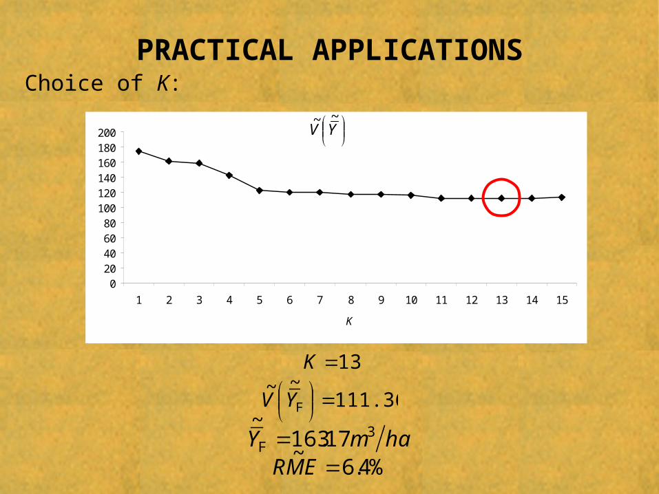
PRACTICAL APPLICATIONSChoice of K:
020406080
100120140160180200
1 2 3 4 5 6 7 8 9 10 11 12 13 14 15
K
YV
~~
ham.Y 317163~
F
111.36~~
FYV
%4.6~
EMR
13K

PRACTICAL APPLICATION
Is the k-NN estimation suitable for this case study?
Check the relationship between Z and Y values

PRACTICAL APPLICATION
Is the k-NN estimation suitable for this case study?
Check the relationship between Z and Y values
Z
Y

Sj
PRACTICAL APPLICATION
Is the k-NN estimation suitable for this case study?
Check the relationship between Z and Y values
Z
Y

Sj
PRACTICAL APPLICATION
Is the k-NN estimation suitable for this case study?
Check the relationship between Z and Y values
Z
Y
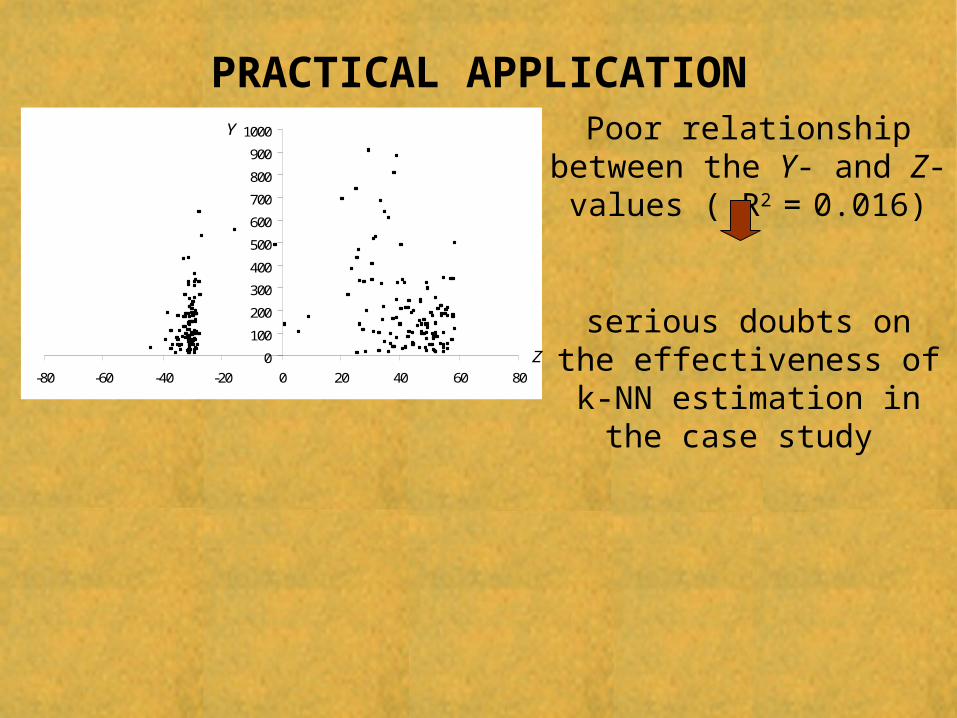
PRACTICAL APPLICATIONPoor relationship between the Y- and Z-values ( R2 = 0.016)
serious doubts on the effectiveness of k-NN
estimation in the case study 0
100
200
300
400
500
600
700
800
900
1000
-80 -60 -40 -20 0 20 40 60 80
Y
Z0
100
200
300
400
500
600
700
800
900
1000
-80 -60 -40 -20 0 20 40 60 80
Y
Z

PRACTICAL APPLICATION
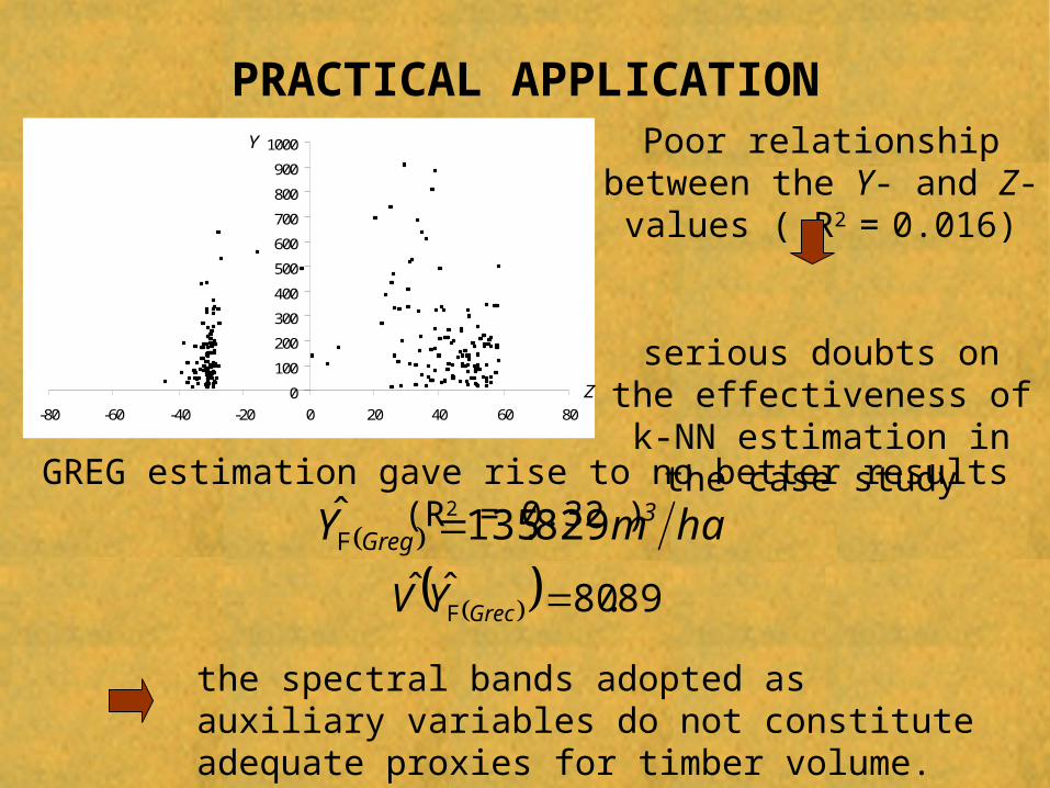
GREG estimation gave rise to no better results (R2 = 0.32 )
ham.Y 3Greg 829135ˆ F
8980ˆˆ .YV Grec F
Poor relationship between the Y- and Z-values ( R2 = 0.016)
serious doubts on the effectiveness of k-NN
estimation in the case study 0
100
200
300
400
500
600
700
800
900
1000
-80 -60 -40 -20 0 20 40 60 80
Y
Z0
100
200
300
400
500
600
700
800
900
1000
-80 -60 -40 -20 0 20 40 60 80
Y
Z
PRACTICAL APPLICATION
the spectral bands adopted as auxiliary variables do not constitute adequate proxies for timber volume.
GREG estimation gave rise to no better results (R2 = 0.32 )
ham.Y 3Greg 829135ˆ F
8980ˆˆ .YV Grec F
Poor relationship between the Y- and Z-values ( R2 = 0.016)
serious doubts on the effectiveness of k-NN
estimation in the case study 0
100
200
300
400
500
600
700
800
900
1000
-80 -60 -40 -20 0 20 40 60 80
Y
Z0
100
200
300
400
500
600
700
800
900
1000
-80 -60 -40 -20 0 20 40 60 80
Y
Z

FINAL REMARKS
• k-NN estimators at the pixel level are generally biased with
mean squared errors which cannot be estimated from the
sample data
FINAL REMARKS
• k-NN estimators at the pixel level are generally biased with
mean squared errors which cannot be estimated from the
sample data
• the linear approximation of is unbiasedY~

FINAL REMARKS
• k-NN estimators at the pixel level are generally biased with
mean squared errors which cannot be estimated from the
sample data
• the linear approximation of is unbiased
• variance estimators are proposed
Y~

FINAL REMARKS
• k-NN estimators at the pixel level are generally biased with
mean squared errors which cannot be estimated from the
sample data
• the linear approximation of is unbiased
• variance estimators are proposed
• a diagnostic tool is proposed
Y~

FINAL REMARKS
• k-NN estimators at the pixel level are generally biased with
mean squared errors which cannot be estimated from the
sample data
• the linear approximation of is unbiased
• variance estimators are proposed
• a diagnostic tool is proposed
• it is stressed to use k-NN method when the neighbouring
structure of pixels in the space of the interest variable is similar
to the neighbouring structure in the space of auxiliary variables
Y~

ReferencesFattorini, L. (2006). Applying the Horvitz-Thompson criterion in complex designs: a computer-intensive perspective for estimating inclusion probabilities. Biometrika, 93, 269-278.
Fattorini, L., & Ridolfi, G. (1997). A sampling design for areal units based on spatial variability. Metron, 55, 59-72.
Fazakas, Z., & Nilsson, M. (1996). Volume of forest cover estimation over southern Sweden using AVHRR data calibrated with TM data. International Journal of Remote Sensing, 17, 1701-1709.
Franco-Lopez, H., Ek, A.R., & Bauer, M. E. (2001). Estimation and mapping of forest stand density, volume, and cover type using the k-nearest Neighbours method. Remote Sensing of Environment, 77, 251-1709.
Haapanen, R., Ek, A. R., Bauer, M. E., & Finley, A. O. (2004). Delineation of forest/nonforest land use classes using nearest neighbours methods. Remote Sensing of Environment, 89, 265-271.
Holmström H., & Fransson, J.E.S. (2003). Combining remotely sensed optical and radar data in k-NN estimation of forest variables. Forest Science, 4, 409-418.
Katila, M., & Tomppo, E. (2001). Selecting estimation parameters for the Finnish multisource National Forest Inventory. Remote Sensing of Environment, 76, 16-32.
Mäkelä, H., & Pekkarinen, A. (2001). Estimation of timber volume at the sample plot level by means of image segmentation and Landsat TM imagery. Remote Sensing of Environment, 77, 66-77.
Mäkelä, H., & Pekkarinen, A. (2004). Estimation of forest stand volume by Landsat TM imagery and stand-level field-inventory data. Forest Ecosystem and Management, 196, 245-255.
McRoberts, R.E., Nelson, M.D., & Wendt, D.G. (2002). Stratified estimation of forest area using satellite imagery, inventory data, and the k-Nearest Neighbours technique. Remote Sensing of Environment, 82, 457-468.
Tokola, T., Pitkänen, J., Partinen, S., & Muinonen, E. (1996). Point accuracy of non-parametic method in estimation of forest characteristics with different satellite materials. International Journal of Remote Sensing, 17, 2333-2351.
Tomppo, E. (1991). Satellite image-based national forest inventory of Finland. International Archives of Photogrammetry and Remote Sensing, 28, 419-424.
Tomppo, E., & Halme, M. (2004). Using course scale forest variables as ancillary information and weighting of variables in k-NN estimation: a genetic algorithm approach. Remote Sensing of Environment, In Press.
Tomppo, E., Nilsson, M., Rosengren, M., Aalto, P., & Kennedy, P. (2002). Simultaneous use of Landsat-TM and IRS-1C WiFS data in estimating large area tree stem volume and aboveground biomass. Remote Sensing of Environment, 82, 156-171.

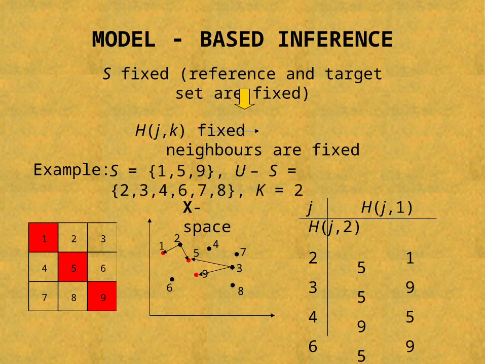
MODEL - BASED INFERENCE
S fixed (reference and target set are fixed)
H(j,k) fixed neighbours are fixed
Example: S = {1,5,9}, U – S = {2,3,4,6,7,8}, K = 2
X-space
12
5
6
47
3
8
9
j H(j,1) H(j,2)
2 1 53 9 54 5 96 9 5 7 5 98 9 5
1 2 3
4 5 6
7 8 9

MODEL - BASED INFERENCE
S fixed (reference and target set are fixed)
H(j,k) fixed neighbours are fixed
Example:
X-space
12
5
6
47
3
8
9
j H(j,1) H(j,2)
2 1 53 9 54 5 96 9 5 7 5 98 9 5
1 2 3
4 5 6
7 8 9
S = {1,5,9}, U – S = {2,3,4,6,7,8}, K = 2
MODEL - BASED INFERENCE
S fixed (reference and target set are fixed)
H(j,k) fixed neighbours are fixed
Example:
X-space
12
5
6
47
3
8
9
j H(j,1) H(j,2)
2 1 53 9 54 5 96 9 5 7 5 98 9 5
1 2 3
4 5 6
7 8 9
S = {1,5,9}, U – S = {2,3,4,6,7,8}, K = 2

MODEL - BASED INFERENCE
S fixed (reference and target set are fixed)
H(j,k) fixed neighbours are fixed
Example:
X-space
12
5
6
47
3
8
9
j H(j,1) H(j,2)
2 1 53 9 54 5 96 9 5 7 5 98 9 5
1 2 3
4 5 6
7 8 9
S = {1,5,9}, U – S = {2,3,4,6,7,8}, K = 2

MODEL - BASED INFERENCE
S fixed (reference and target set are fixed)
H(j,k) fixed neighbours are fixed
Example:
X-space
12
5
6
47
3
8
9
j H(j,1) H(j,2)
2 1 53 9 54 5 96 9 5 7 5 98 9 5
1 2 3
4 5 6
7 8 9
S = {1,5,9}, U – S = {2,3,4,6,7,8}, K = 2

MODEL - BASED INFERENCE
S fixed (reference and target set are fixed)
H(j,k) fixed neighbours are fixed
Example:
X-space
12
5
6
47
3
8
9
j H(j,1) H(j,2)
2 1 53 9 54 5 96 9 5 7 5 98 9 5
1 2 3
4 5 6
7 8 9
S = {1,5,9}, U – S = {2,3,4,6,7,8}, K = 2

MODEL - BASED INFERENCE
S fixed (reference and target set are fixed)
H(j,k) fixed neighbours are fixed
Example:
X-space
12
5
6
47
3
8
9
j H(j,1) H(j,2)
2 1 53 9 54 5 96 9 5 7 5 98 9 5
1 2 3
4 5 6
7 8 9
S = {1,5,9}, U – S = {2,3,4,6,7,8}, K = 2

MODEL - BASED INFERENCEMcRoberts – Tomppo – Finley – Heikkinen (2007)
jjjy
0jE 2jjV hjjhhjCov ,

MODEL - BASED INFERENCEMcRoberts – Tomppo – Finley – Heikkinen (2007)
jjjy
0jE 2jjV hjjhhjCov ,
BASIC ASSUMPTION
KkyEyE kjHj ,...,2,1,
neighbouring units have similar expectations
K-NN is a model-unbiased prediction
0|~ SyyE jjY
1.
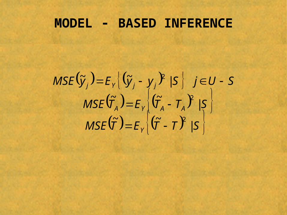
MODEL - BASED INFERENCE
STTETMSE
STTETMSE
SUjSyyEyMSE
Y
AAYA
jjYj
|~~
|~~
|~~
2
2
2

MODEL - BASED INFERENCEList of assumptions:
2. A parametric structure of covariance function (variogram)
3. See Appendix 1 (McRoberts, R. E. et al., 2007)
3a)
3b)
3c)
3d)
2
1
2),(
1j
K
kkjHk
2
1 1')',(),(2
1j
K
k
K
kkjHkjHk
2
1
2),(
1j
K
kkjHk
KkjkjHkjH ,...,2,12)',(),(

MODEL - BASED INFERENCE4. See Appendix 3 (McRoberts, R. E. et al., 2007)
KkjkjH ,...,2,1),(

MODEL - BASED INFERENCE
KkjkjH ,...,2,1),(
assumption 1 and 4 involve 3
neighbouring units have similar mean and variances
4. See Appendix 3 (McRoberts, R. E. et al., 2007)

MODEL - BASED INFERENCE
ARE THESE ASSUMPTIONS REALISTIC?
KkjkjH ,...,2,1),(
assumption 1 and 4 involve 3
neighbouring units have similar mean and variances
4. See Appendix 3 (McRoberts, R. E. et al., 2007)
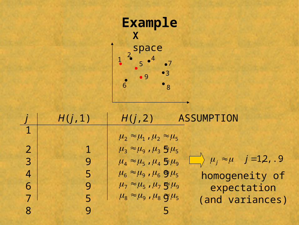
Example
j H(j,1) H(j,2) ASSUMPTION 1
2 1 53 9 54 5 96 9 5 7 5 98 9 5
X space
12
5
6
47
3
8
9
5212 ,
5393 ,
9454 , 5696 , 9757 , 5898 ,
9,...,2,1 jj
homogeneity of expectation (and
variances)
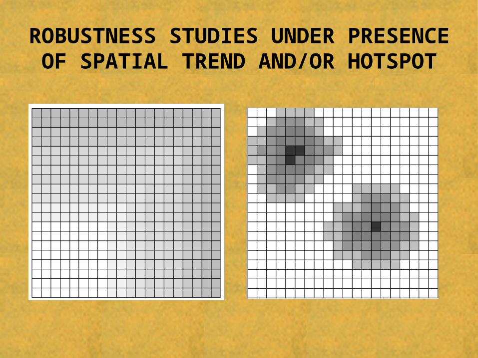
ROBUSTNESS STUDIES UNDER PRESENCE OF SPATIAL TREND AND/OR HOTSPOT