A Description of the Nonhydrostatic Regional COSMO-Model ...version is running operationally at DWD...
181
Consortium for Small-Scale Modelling A Description of the Nonhydrostatic Regional COSMO-Model Part VII : User’s Guide U. Sch¨ attler, G. Doms, and C. Schraff COSMO V5.05 April 2018 www.cosmo-model.org Printed at Deutscher Wetterdienst, P.O. Box 100465, 63004 Offenbach, Germany
Transcript of A Description of the Nonhydrostatic Regional COSMO-Model ...version is running operationally at DWD...
Consortium for Small-Scale Modelling
A Description of the
Nonhydrostatic Regional COSMO-Model
Part VII :
User’s Guide
U. Schattler, G. Doms, and C. Schraff
COSMO V5.05 April 2018
www.cosmo-model.org
Printed at Deutscher Wetterdienst, P.O. Box 100465, 63004 Offenbach, Germany


Contents i
Contents
1 Overview on the Model System 1
1.1 General Remarks . . . . . . . . . . . . . . . . . . . . . . . . . . . . . . . . . . 1
1.2 Basic Model Design and Features . . . . . . . . . . . . . . . . . . . . . . . . . 3
1.3 Organization of the Documentation . . . . . . . . . . . . . . . . . . . . . . . . 7
2 Introduction 8
3 Model Formulation and Data Assimilation 10
3.1 Basic State and Coordinate-System . . . . . . . . . . . . . . . . . . . . . . . . 10
3.2 Differential Form of Thermodynamic Equations . . . . . . . . . . . . . . . . . 12
3.3 Horizontal and Vertical Grid Structure . . . . . . . . . . . . . . . . . . . . . . 13
3.4 Numerical Integration . . . . . . . . . . . . . . . . . . . . . . . . . . . . . . . 16
3.4.1 Runge-Kutta: 2-timelevel HE-VI Integration . . . . . . . . . . . . . . 17
3.4.2 Leapfrog: 3-timelevel HE-VI Integration . . . . . . . . . . . . . . . . . 18
3.4.3 Leapfrog: 3-timelevel Semi-Implicit Integration . . . . . . . . . . . . . 18
3.5 Physical Parameterizations . . . . . . . . . . . . . . . . . . . . . . . . . . . . 19
3.5.1 Radiation . . . . . . . . . . . . . . . . . . . . . . . . . . . . . . . . . . 19
3.5.2 Grid-scale Precipitation . . . . . . . . . . . . . . . . . . . . . . . . . . 19
3.5.3 Moist Convection . . . . . . . . . . . . . . . . . . . . . . . . . . . . . . 21
3.5.4 Vertical Turbulent Diffusion . . . . . . . . . . . . . . . . . . . . . . . . 23
3.5.5 Parameterization of Surface Fluxes . . . . . . . . . . . . . . . . . . . . 24
3.5.6 A subgrid-scale orography scheme . . . . . . . . . . . . . . . . . . . . 24
3.5.7 Soil Processes . . . . . . . . . . . . . . . . . . . . . . . . . . . . . . . . 24
3.6 Data Assimilation . . . . . . . . . . . . . . . . . . . . . . . . . . . . . . . . . 27
Part VII – User’s Guide 5.05 Contents
Contents ii
4 Installation of the COSMO-Model 29
4.1 External Libraries for the COSMO-Model . . . . . . . . . . . . . . . . . . . . 29
4.1.1 libgrib1.a: . . . . . . . . . . . . . . . . . . . . . . . . . . . . . . . . 29
4.1.2 libgrib api.a, libgrib api f90.a: . . . . . . . . . . . . . . . . . . 30
4.1.3 libnetcdf.a: . . . . . . . . . . . . . . . . . . . . . . . . . . . . . . . . 30
4.1.4 libmisc.a: . . . . . . . . . . . . . . . . . . . . . . . . . . . . . . . . . 30
4.1.5 libcsobank.a, libsupplement.a: . . . . . . . . . . . . . . . . . . . . 31
4.1.6 libRTTOVxx.a: . . . . . . . . . . . . . . . . . . . . . . . . . . . . . . . 31
4.2 Preparing the Code . . . . . . . . . . . . . . . . . . . . . . . . . . . . . . . . . 32
4.3 Compiling and Linking . . . . . . . . . . . . . . . . . . . . . . . . . . . . . . . 32
4.4 Running the Code . . . . . . . . . . . . . . . . . . . . . . . . . . . . . . . . . 33
5 Input Files for the COSMO-Model 34
5.1 Files for Namelist Input . . . . . . . . . . . . . . . . . . . . . . . . . . . . . . 34
5.2 Conventions for File Names . . . . . . . . . . . . . . . . . . . . . . . . . . . . 36
5.3 Initial and Boundary Data . . . . . . . . . . . . . . . . . . . . . . . . . . . . . 38
5.4 Observation Input Files . . . . . . . . . . . . . . . . . . . . . . . . . . . . . . 40
5.4.1 Templates for observation types for which Table-Driven Code Forms(TDCF) defined by WMO exist . . . . . . . . . . . . . . . . . . . . . . 42
5.4.2 Observation types with templates proposed or approved by WMO . . 51
5.4.3 Observation types without templates proposed by WMO . . . . . . . 57
5.4.4 The blacklist file . . . . . . . . . . . . . . . . . . . . . . . . . . . . . . 60
6 Namelist Input for COSMO-Model 63
6.1 LMGRID — Model Domain and Reference Atmosphere . . . . . . . . . . . . . . 66
6.2 RUNCTL — Parameters for the Model Run . . . . . . . . . . . . . . . . . . . . 68
6.3 DYNCTL — Parameters for the Adiabatic Model . . . . . . . . . . . . . . . . . 79
6.4 PHYCTL — Parameters for the Diabatic Model . . . . . . . . . . . . . . . . . . 90
6.4.1 Different Configurations for the COSMO-ICON Physics . . . . . . . . 107
6.5 TUNING — Parameters for tuning dynamics and physics . . . . . . . . . . . . 113
6.6 DIACTL — Parameters for Diagnostic Output . . . . . . . . . . . . . . . . . . 119
6.7 SATCTL — Controlling the Synthetic Satellite Images . . . . . . . . . . . . . . 122
Part VII – User’s Guide 5.05 Contents
Contents iii
6.8 INICTL — Parameters for the Model Initialization . . . . . . . . . . . . . . . 126
6.9 EPSCTL — Controlling the Ensemble Prediction Mode . . . . . . . . . . . . . 128
6.10 IOCTL — Controlling the Grib I/O . . . . . . . . . . . . . . . . . . . . . . . . 132
6.11 DATABASE — Specification of Database Job . . . . . . . . . . . . . . . . . . . 136
6.12 GRIBIN — Controlling the Grib Input . . . . . . . . . . . . . . . . . . . . . . 137
6.13 GRIBOUT — Controlling the Grib Output . . . . . . . . . . . . . . . . . . . . . 141
7 Namelist Input for Data Assimilation 146
7.1 NUDGING — Controlling the Data Assimilation . . . . . . . . . . . . . . . . . . 146
8 Special Operators for the Data Assimilation 169
8.1 The GNSS STD Operator . . . . . . . . . . . . . . . . . . . . . . . . . . . . . 169
8.1.1 Input for the GNSS STD Operator . . . . . . . . . . . . . . . . . . . . 169
8.1.2 STD OBS — Parameter for the GNSS STD Operator . . . . . . . . . . 170
References 173
Part VII – User’s Guide 5.05 Contents

Contents iv
Part VII – User’s Guide 5.05 Contents
1
Section 1
Overview on the Model System
1.1 General Remarks
The COSMO-Model is a nonhydrostatic limited-area atmospheric prediction model. It hasbeen designed for both operational numerical weather prediction (NWP) and various scien-tific applications on the meso-β and meso-γ scale. The COSMO-Model is based on the prim-itive thermo-hydrodynamical equations describing compressible flow in a moist atmosphere.The model equations are formulated in rotated geographical coordinates and a generalizedterrain following height coordinate. A variety of physical processes are taken into account byparameterization schemes.
Besides the forecast model itself, a number of additional components such as data assimi-lation, interpolation of boundary conditions from a driving host model, and postprocessingutilities are required to run the model in NWP-mode, climate mode or for case studies. Thepurpose of the Description of the Nonhydrostatic Regional COSMO-Model is to provide acomprehensive documentation of all components of the system and to inform the user aboutcode access and how to install, compile, configure and run the model.
The basic version of the COSMO-Model (formerly known as Lokal Modell (LM)) has beendeveloped at the Deutscher Wetterdienst (DWD). The COSMO-Model and the triangularmesh global gridpoint model ICON form – together with the corresponding data assimi-lation schemes – the NWP-system at DWD. The subsequent developments related to theCOSMO-Model have been organized within ”COSMO”, the Consortium for Small-ScaleModeling. COSMO aims at the improvement, maintenance and operational applicationof a non-hydrostatic limited-area modeling system, which is now consequently called theCOSMO-Model. The meteorological services participating to COSMO at present are listedin Table 1.1.
For more information about COSMO, we refer to the web-site at www.cosmo-model.org .
The COSMO-Model is available free of charge for scientific and educational purposes, es-pecially for cooperational projects with COSMO members. However, all users are requiredto sign an agreement with a COSMO national meteorological service and to respect cer-tain conditions and restrictions on code usage. For questions concerning the request and theagreement, please contact the chairman of the COSMO Steering Committee. In the case ofa planned operational or commercial use of the COSMO-Model package, special regulations
Part VII – User’s Guide 5.05 Section 1: Overview on the Model System

1.1 General Remarks 2
Table 1.1: COSMO: Participating Meteorological Services
DWD Deutscher Wetterdienst,Offenbach, Germany
MeteoSwiss Meteo-Schweiz,Zurich, Switzerland
USAM Ufficio Generale Spazio Aero e Meteorologia,Roma, Italy
HNMS Hellenic National Meteorological Service,Athens, Greece
IMGW Institute of Meteorology and Water Management,Warsaw, Poland
ARPA-SIMC Agenzia Regionale per la Protezione Ambientale dellEmilia-Romagna Servizio Idro Meteo ClimaBologna, Italy
ARPA-Piemonte Agenzia Regionale per la Protezione Ambientale,Piemonte, Italy
CIRA Centro Italiano Ricerche Aerospaziali,Italy
ZGeoBW Zentrum fur Geoinformationswesen der Bundeswehr,Euskirchen, Germany
NMA National Meteorological Administration,Bukarest, Romania
RosHydroMet Hydrometeorological Centre of Russia,Moscow, Russia
RosHydroMet Israel Meteorological Service,Bet-Dagan, Israel
will apply.
The further development of the modeling system within COSMO is organized in WorkingGroups which cover the main research and development activities: data assimilation, nu-merical aspects, upper air physical aspects, soil and surface physics aspects, interpretationand applications, verification and case studies, reference version and implementation andpredictability and ensemble methods. In 2005, the COSMO Steering Committee decided todefine Priority Projects with the goal to focus the scientific activities of the COSMO com-munity on some few key issues and support the permanent improvement of the model. Forcontacting the Working Group Coordinators or members of the Working Groups or PriorityProjects, please refer to the COSMO web-site.
The COSMO meteorological services are not equipped to provide extensive support to ex-ternal users of the model. If technical problems occur with the installation of the modelsystem or with basic questions how to run the model, questions could be directed via emailto [email protected]. If further problems occur, please contact the membersof an appropriate Working Group. We try to assist you as well as possible.
The authors of this document recognize that typographical and other errors as well as dis-
Part VII – User’s Guide 5.05 Section 1: Overview on the Model System
1.2 Basic Model Design and Features 3
crepancies in the code and deficiencies regarding the completeness may be present, and yourassistance in correcting them is appreciated. All comments and suggestions for improvementor corrections of the documentation and the model code are welcome and may be directedto the authors.
1.2 Basic Model Design and Features
The nonhydrostatic fully compressible COSMO-Model has been developed to meet high-resolution regional forecast requirements of weather services and to provide a flexible toolfor various scientific applications on a broad range of spatial scales. When starting withthe development of the COSMO-Model, many NWP-models operated on hydrostatic scalesof motion with grid spacings down to about 10 km and thus lacked the spatial resolutionrequired to explicitly capture small-scale severe weather events. The COSMO-Model hasbeen designed for meso-β and meso-γ scales where nonhydrostatic effects begin to play anessential role in the evolution of atmospheric flows.
By employing 1 to 3 km grid spacing for operational forecasts over a large domain, it isexpected that deep moist convection and the associated feedback mechanisms to the largerscales of motion can be explicitly resolved. Meso-γ scale NWP-models thus have the princi-ple potential to overcome the shortcomings resulting from the application of parameterizedconvection in current coarse-grid hydrostatic models. In addition, the impact of topographyon the organization of penetrative convection by, e.g. channeling effects, is represented muchmore realistically in high resolution nonhydrostatic forecast models.
In the beginning, the operational application of the model within COSMO were mainly onthe meso-β scale using a grid spacing of 7 km. The key issue was an accurate numericalprediction of near-surface weather conditions, focusing on clouds, fog, frontal precipitation,and orographically and thermally forced local wind systems. Since April 2007, a meso-γ scaleversion is running operationally at DWD by employing a grid spacing of 2.8 km. Applicationswith similar resolutions are now run by most COSMO partners. We expect that this willallow for a direct simulation of severe weather events triggered by deep moist convection,such as supercell thunderstorms, intense mesoscale convective complexes, prefrontal squall-line storms and heavy snowfall from wintertime mesocyclones.
The requirements for the data assimilation system for the operational COSMO-Model aremainly determined by the very high resolution of the model and by the task to employ italso for nowcasting purposes in the future. Hence, detailed high-resolution analyses have tobe able to be produced frequently and quickly, and this requires a thorough use of asynopticand high-frequency observations such as aircraft data and remote sensing data. Since both3-dimensional and 4-dimensional variational methods tend to be less appropriate for thispurpose, a scheme based on the observation nudging technique has been chosen for dataassimilation.
Besides the operational application, the COSMO-Model provides a nonhydrostatic model-ing framework for various scientific and technical purposes. Examples are applications ofthe model to large-eddy simulations, cloud resolving simulations, studies on orographic flowsystems and storm dynamics, development and validation of large-scale parameterizationschemes by fine-scale modeling, and tests of computational strategies and numerical tech-niques. For these types of studies, the model should be applicable to both real data cases
Part VII – User’s Guide 5.05 Section 1: Overview on the Model System

1.2 Basic Model Design and Features 4
and artificial cases using idealized test data. Moreover, the model has been adapted by othercommunities for applications in climate mode (CCLM) and / or running an online coupledmodule for aerosols and reactive trace gases (ART).
Such a wide range of applications imposes a number of requirements for the physical, nu-merical and technical design of the model. The main design requirements are:
(i) use of nonhydrostatic, compressible dynamical equations to avoid restrictions on thespatial scales and the domain size, and application of an efficient numerical method ofsolution;
(ii) provision of a comprehensive physics package to cover adequately the spatial scalesof application, and provision of high-resolution data sets for all external parametersrequired by the parameterization schemes;
(iii) flexible choice of initial and boundary conditions to accommodate both real data casesand idealized initial states, and use of a mesh-refinement technique to focus on regionsof interest and to handle multi-scale phenomena;
(iv) use of a high-resolution analysis method capable of assimilating high-frequency asyn-optic data and remote sensing data;
(v) use of pure Fortran constructs to render the code portable among a variety of com-puter systems, and application of the standard MPI-software for message passing ondistributed memory machines to accommodate broad classes of parallel computers.
The development of the COSMO-Model was organized along these basic guidelines. How-ever, not all of the requirements are fully implemented, and development work and furtherimprovement is an ongoing task. The main features and characteristics of the present releaseare summarized below.
Dynamics
- Model Equations – Nonhydrostatic, full compressible hydro-thermodynamical equations inadvection form. Subtraction of a hydrostatic base state at rest.
- Prognostic Variables – Horizontal and vertical Cartesian wind components, pressure per-turbation, temperature, specific humidity, cloud water content. Optionally: cloud ice content,turbulent kinetic energy, specific water content of rain, snow and graupel.
- Diagnostic Variables – Total air density, precipitation fluxes of rain and snow.
- Coordinate System – Generalized terrain-following height coordinate with rotated geograph-ical coordinates and user defined grid stretching in the vertical. Options for (i) base-statepressure based height coordinate, (ii) Gal-Chen height coordinate and (iii) exponential heightcoordinate (SLEVE) according to Schaer et al. (2002).
Numerics
- Grid Structure – Arakawa C-grid, Lorenz vertical grid staggering.
- Spatial Discretization – Second-order finite differences. For the two time-level scheme also1st and 3rd to 6th order horizontal advection (default: 5th order). Option for explicit higherorder vertical advection.
Part VII – User’s Guide 5.05 Section 1: Overview on the Model System
1.2 Basic Model Design and Features 5
- Time Integration – Two time-level 2nd and 3rd order Runge-Kutta split-explicit scheme afterWicker and Skamarock (2002) and a TVD-variant (Total Variation Diminishing) of a 3rd orderRunge-Kutta split-explicit scheme. Option for a second-order leapfrog HE-VI (horizontallyexplicit, vertically implicit) time-split integration scheme, including extensions proposed bySkamarock and Klemp (1992). Option for a three time-level 3-d semi-implicit scheme (Thomaset al. (2000)) based on the leapfrog scheme.
- Numerical Smoothing – 4th-order linear horizontal diffusion with option for a monotonic ver-sion including an orographic limiter. Rayleigh damping in upper layers. 2-d divergence dampingand off-centering in the vertical in split time steps.
Initial and Boundary Conditions
- Initial Conditions – Interpolated initial data from various coarse-grid driving models (ICON(and former GME), ECMWF, COSMO-Model) or from the continuous data assimilation stream(see below). Option for user-specified idealized initial fields.
- Lateral Boundary Conditions – 1-way nesting by Davies-type lateral boundary formula-tion. Data from several coarse-grid models can be processed (ICON (and former GME), IFS,COSMO-Model). Option for periodic boundary conditions.
- Top Boundary Conditions – Options for rigid lid condition and Rayleigh damping layer.
- Initialization – Digital-filter initialization of unbalanced initial states (Lynch et al. (1997))with options for adiabatic and diabatic initialization.
Physical Parameterizations
- Subgrid-Scale Turbulence – Prognostic turbulent kinetic energy closure at level 2.5 includingeffects from subgrid-scale condensation and from thermal circulations. Option for a diagnosticsecond order K-closure of hierarchy level 2 for vertical turbulent fluxes. Preliminary option forcalculation of horizontal turbulent diffusion in terrain following coordinates (3D Turbulence).
- Surface Layer Parameterization – A Surface layer scheme (based on turbulent kineticenergy) including a laminar-turbulent roughness layer. Option for a stability-dependent drag-law formulation of momentum, heat and moisture fluxes according to similarity theory (Louis(1979)).
- Grid-Scale Clouds and Precipitation – Cloud water condensation and evaporation by sat-uration adjustment. Precipitation formation by a bulk microphysics parameterization includingwater vapour, cloud water, cloud ice, rain and snow with 3D transport for the precipitatingphases. Option for a new bulk scheme including graupel. Option for a simpler column equilib-rium scheme.
- Subgrid-Scale Clouds – Subgrid-scale cloudiness is interpreted by an empirical functiondepending on relative humidity and height. A corresponding cloud water content is also inter-preted. Option for a statistical subgrid-scale cloud diagnostic for turbulence.
- Moist Convection – Tiedtke (1989) mass-flux convection scheme with equilibrium closurebased on moisture convergence. Option for the current IFS Tiedtke-Bechtold convection scheme.
- Shallow Convection – Reduced Tiedtke scheme for shallow convection only.
- Radiation – δ two-stream radiation scheme after Ritter and Geleyn (1992) short and longwavefluxes (employing eight spectral intervals); full cloud-radiation feedback.
- Soil Model – Multi-layer version of the former two-layer soil model after Jacobsen and Heise(1982) based on the direct numerical solution of the heat conduction equation. Snow andinterception storage are included.
- Fresh-Water Lake Parameterization – Two-layer bulk model after Mironov (2008) topredict the vertical temperature structure and mixing conditions in fresh-water lakes of variousdepths.
Part VII – User’s Guide 5.05 Section 1: Overview on the Model System
1.2 Basic Model Design and Features 6
- Sea-Ice Scheme – Parameterization of thermodynamic processes (without rheology) afterMironov and B. (2004). The scheme basically computes the energy balance at the ices surface,using one layer of sea ice.
- Terrain and Surface Data – All external parameters of the model are available at variousresolutions for a pre-defined region covering Europe. For other regions or grid-spacings, theexternal parameter file can be generated by a preprocessor program using high-resolution globaldata sets.
Data Assimilation
- Basic Method – Continuous four-dimensional data assimilation based on observation nudg-ing (Schraff (1996), Schraff (1997)), with lateral spreading of upper-air observation incrementsalong horizontal surfaces. Explicit balancing by a hydrostatic temperature correction for sur-face pressure updates, a geostrophic wind correction, and a hydrostatic upper-air pressurecorrection.
- Assimilated Atmospheric Observations – Radiosonde (wind, temperature, humidity), air-craft (wind, temperature), wind profiler (wind), and surface-level data (SYNOP, SHIP, BUOY:pressure, wind, humidity). Optionally RASS (temperature), radar VAD wind, and ground-basedGPS (integrated water vapour) data. Surface-level temperature is used for the soil moistureanalysis only.
- Radar derived rain rates – Assimilation of near surface rain rates based on latent heatnudging (Stephan et al. (2008)). It locally adjusts the three-dimensional thermodynamical fieldof the model in such a way that the modelled precipitation rates should resemble the observedones.
- Surface and Soil Fields – Additional two-dimensional intermittent analysis:
- Soil Moisture Analysis – Daily adjustment of soil moisture by a variational method(Hess (2001)) in order to improve 2-m temperature forecasts; use of a Kalman-Filter-likebackground weighting.
- Sea Surface Temperature Analysis – Daily Cressman-type correction, and blendingwith global analysis. Use of external sea ice cover analysis.
- Snow Depth Analysis – 6-hourly analysis by weighted averaging of snow depth obser-vations, and use of snowfall data and predicted snow depth.
Code and Parallelization
- Code Structure – Modular code structure using standard Fortran constructs.
- Parallelization – The parallelization is done by horizontal domain decomposition using asoft-coded gridline halo (2 lines for Leapfrog, 3 for the Runge-Kutta scheme). The MessagePassing Interface software (MPI) is used for message passing on distributed memory machines.
- Compilation of the Code – For all programs a Makefile is provided for the compilation whichis invoked by the Unix make command. Two files are belonging to the Makefile: ObjFiles isa list of files that have to be compiled and ObjDependencies contains all file dependencies. Inaddition it reads the file Fopts, which has to be adapted by the user to specify the compiler,compiler options and necessary libraries to link.
- Portability – The model can be easily ported to various platforms; current applications are onconventional scalar machines (UNIX workstations, LINUX and Windows-NT PCs), on vectorcomputers (NEC SX series) and MPP machines (CRAY, IBM, SGI and others).
- Model Geometry – 3-d, 2-d and 1-d model configurations. Metrical terms can be adjustedto represent tangential Cartesian geometry with constant or zero Coriolis parameter.
Part VII – User’s Guide 5.05 Section 1: Overview on the Model System
1.3 Organization of the Documentation 7
Table 1.2: COSMO Documentation: A Description of the Nonhydrostatic Regional COSMO-Model
Part I: Dynamics and Numerics
Part II: Physical Parameterization
Part III: Data Assimilation
Part IV: Special Components and Implementation Details
Part V: Preprocessing: Initial and Boundary Data for theCOSMO-Model
Part VI: Model Output and Data Formats for I/O
Part VII: User’s Guide
1.3 Organization of the Documentation
For the documentation of the model we follow closely the European Standards for Writing andDocumenting Exchangeable Fortran 90-Code. These standards provide a framework for theuse of Fortran-90 in European meteorological organizations and weather services and therebyfacilitate the exchange of code between these centres. According to these standards, themodel documentation is split into two categories: external documentation (outside the code)and internal documentation (inside the code). The model provides extensive documentationwithin the codes of the subroutines. This is in form of procedure headers, section commentsand other comments. The external documentation is split into seven parts, which are listedin Table 1.2.
Parts I - III form the scientific documentation, which provides information about the theo-retical and numerical formulation of the model, the parameterization of physical processesand the four-dimensional data assimilation. The scientific documentation is independent of(i.e. does not refer to) the code itself. Part IV will describe the particular implementationof the methods and algorithms as presented in Parts I - III, including information on thebasic code design and on the strategy for parallelization using the MPI library for messagepassing on distributed memory machines (not available yet). The generation of initial andboundary conditions from coarse grid driving models is described in Part V. This part is adescription of the interpolation procedures and algorithms used (not yet complete) as wellas a User’s Guide for the interpolation program INT2LM. In Part VI we give a descriptionof the data formats, which can be used in the COSMO-Model, and describe the outputfrom the model and from data assimilation. Finally, the User’s Guide of the COSMO-Modelprovides information on code access and how to install, compile, configure and run themodel. The User’s Guide contains also a detailed description of various control parametersin the model input file (in NAMELIST format) which allow for a flexible model set-up forvarious applications. All parts of the documentation are available at the COSMO web-site(http://www.cosmo-model.org/content/model/documentation/core/default.htm).
Part VII – User’s Guide 5.05 Section 1: Overview on the Model System
8
Section 2
Introduction
The usage of the program package for the COSMO-Model is a rather complex task, both,for the experienced and even more for the non-experienced user. This User’s Guide serves ina first instance as a complete reference for all the different NAMELIST groups and variables,with which the execution of the model can be controlled.
But first, an overview on the model formulation and the data assimilation is given in Section3. The installation of the package is explained in Section 4, which also gives information onexternal libraries used in the COSMO-Model. Necessary input files of the model are listedin Section 5 and the detailed descriptions of all NAMELIST variables are given in Sections 6and 7.
Knowing the meaning of all NAMELIST-variables normally is not enough to find the waythrough the possible configurations of the model. Therefore, a description would be desirablethat explains how the variables can be put together to give a meaningful setup, or whichvariable settings contradict each other or simply are not possible. Such a description is notavailable, but we tried to indicate dependencies of variables in the descriptions in Section6. We also refer to the web-page of the CLM Community. They implemented a NAMELIST-tool, where you can find different practical setups for the climate and for the NWP mode:(http://www.clm-community.eu/namelist-tool/namelist-tool portal/index.htm).
Part VII – User’s Guide 5.05 Section 2: Introduction

9
Figure 2.1: Schematic view of the different COSMO-Model components
Dynamics
#
"
!
2 time levelsplit-explicitRunge-Kutta(several vari-ants)
��
��
3 time levelsplit-explicitLeapfrog
��
��
3 time levelsemi-implicitLeapfrog
�
�Relaxation
Physics
'
&
$
%
Grid Scale Clouds andPrecipitation (with 3Dtransport of precipitat-ing particles)- warm rain scheme- 1-category ice scheme- 2-category ice scheme- 3-category ice scheme
�
�Radiation
'
&
$
%
Subgrid Scale Turbu-lence Closure- 1-D diag. closure- 1-D TKE-based
diagnostic closure- 3-D TKE-based
prognostic closure
'
&
$
%
Parameterization ofSurface Fluxes- Standard bulk trans-
fer scheme- TKE-based surface
scheme
�
�
�
�Moist Convection- Tiedtke mass-flux- Tiedtke-Bechtold- Shallow convection
�
�Subgrid sc. orography
�
�
�
�Soil and Surface- multi-layer soil- lake model- sea-ice scheme
Assimilation
��
��
Observationprocessing
�
�Surface analysis
�
�
�
�Nudging of atmo-spheric variablesand surface pres-sure
��
��
Latent HeatNudging
Initialization
�
�Digital filtering
Diagnostics
��
��
Near surfaceweatherparameters
�
�Mean values
�
�Meteographs
��
��
Volume- andArea-Integrals
��
�
Synthetic Sa-tellite Pictures
I/O
�
�Grib
�
�NetCDF
�
�Restart
Part VII – User’s Guide 5.05 Section 2: Introduction

10
Section 3
Model Formulation and DataAssimilation
3.1 Basic State and Coordinate-System
The COSMO-Model is based on the primitive hydro-thermodynamical equations describingcompressible nonhydrostatic flow in a moist atmosphere without any scale approximations.A basic state is subtracted from the equations to reduce numerical errors associated withthe calculation of the pressure gradient force in case of sloping coordinate surfaces. Thebasic state represents a time-independent dry atmosphere at rest which is prescribed to behorizontally homogeneous, vertically stratified and in hydrostatic balance.
By introducing the basic state, the thermodynamic variables temperature (T ), pressure (p)and density (ρ) can be formally written as the sum of a height dependent reference valueand a space and time dependent deviation:
T = T0(z) + T ′, p = p0(z) + p′, ρ = ρ0(z) + ρ′ , (3.1)
where T0(z), p0(z) and ρ0(z) are related by the hydrostatic equation
∂p0∂z
= −gρ0 = − gp0RdT0
(3.2)
and the equation of state, p0 = ρ0RdT0. Rd is the gas constant of dry air. The vertical profileT0(z) of temperature can be specified arbitrary since we do not linearize the model equationswith respect to the reference state.
In the first implementation of the COSMO-Model we prescribed a constant rate β forthe temperature increase with the logarithm of pressure (as proposed by Dudhia (1993)),∂T0/∂ ln p0 = β. The integration of the hydrostatic equation (3.2) with the boundary valuespSL = p0 (z = 0) and TSL = T0 (z = 0) for the pressure and temperature at mean sea levelz = 0 then yields the vertical profiles of the reference state:
p0(z) =
pSL exp
{−TSL
β
(1−
√1− 2βgz
RdT2SL
)}if β 6= 0
pSL exp{− gzRdTSL
}if β = 0
Part VII – User’s Guide 5.05 Section 3: Model Formulation and Data Assimilation

3.1 Basic State and Coordinate-System 11
(3.3)
T0(z) = TSL
√1− 2βgz
RdT2SL
.
For the three parameters pSL, TSL and β, which define the basic state, we use the defaultvalues pSL = 1000hPa, TSL = 288.15K and β = 42K. The variable names in the programsare p0sl (pSL), t0sl (TSL) and dt0lp (β), resp. This basic state is still available in theCOSMO-Model and can be chosen as Reference Atmosphere 1 (irefatm=1).
Since COSMO-Model 4.5, a new alternative reference atmosphere has been implemented,which can be chosen as Reference Atmosphere 2 (irefatm=2). This reference atmosphere isbased on the temperature profile
T0(z) = T00 + δT · exp(−z/hscal), (3.4)
with default values of T00 = 213.15K, δT = 75K and hscal = 10km. In the model code,T00 = TSL−δT = t0sl - delta t. Thus, the reference atmosphere approaches an isothermalprofile in the stratosphere, whereas the existing reference profile has an increasingly negativevertical temperature gradient in the stratosphere. The vertical extent of the model domainis no longer limited with the new reference atmosphere.
The new reference atmosphere needs two additional parameters δT (model variable delta t)and hscal (model variable h scal). Default values are delta t=75.0 and h scal=10000.0,resp.
The model equations are formulated with respect to a rotated lat/lon-grid with coordinates(λ, ϕ). The rotated coordinate system results from the geographical (λg, ϕg) coordinatesby tilting the north pole (see Part I of the Documentation, Dynamics and Numerics). Inthe vertical, we use a generalized terrain-following height coordinate ζ, where any uniquefunction of geometrical height can be used for transformation. Since ζ doesn’t depend ontime, the (λ, ϕ,ζ)-system represents a non-deformable coordinate system, where surfaces ofconstant ζ are fixed in space - in contrast to the pressure based coordinate system of mosthydrostatic models, where the surfaces of constant vertical coordinate move in space withchanging surface pressure.
The transformation of the model equations from the orthogonal (λ, ϕ, z)-system to the non-orthogonal terrain-following (λ, ϕ, ζ)-system is given by the three elements of the inverseJacobian matrix J z,
Jλ ≡ Jz13 =
(∂z
∂λ
)ζ, Jϕ ≡ Jz23 =
(∂z
∂ϕ
)ζ
, Jζ ≡ Jz33 =∂z
∂ζ= −√G. (3.5)
The terrain-following ζ-system of the COSMO-Model is defined to be left-handed, i.e. thevalue of the ζ-coordinate increases with decreasing height z from the top of the model tothe surface. Thus, Jζ is always negative and equal to the negative absolute value (
√G =
|det (J z) |) of the determinant of the inverse Jacobi matrix.
Part VII – User’s Guide 5.05 Section 3: Model Formulation and Data Assimilation

3.2 Differential Form of Thermodynamic Equations 12
3.2 Differential Form of Thermodynamic Equations
By transforming the primitive hydro-thermodynamical equations to the (λ, ϕ, ζ) coordinate-system and subtracting the basic state, we achieve the following set of prognostic modelequations for the three components u, v and w of the wind vector, the perturbation pressurep′, the temperature T and the humidity variables q.
∂u
∂t+ v · ∇u− uv
atanϕ− fv = − 1
ρa cosϕ
(∂p′
∂λ+
Jλ√G
∂p′
∂ζ
)+Mu
∂v
∂t+ v · ∇v +
u2
atanϕ+ fu = − 1
ρa
(∂p′
∂ϕ+
Jϕ√G
∂p′
∂ζ
)+Mv
∂w
∂t+ v · ∇w =
1
ρ√G
∂p′
∂ζ+B +Mw (3.6)
∂p′
∂t+ v · ∇p′ − gρ0w = −(cpd/cvd)pD
∂T
∂t+ v · ∇T = − p
ρcvdD +QT
∂qv
∂t+ v · ∇qv = −(Sl + Sf ) +Mqv
∂ql,f
∂t+ v · ∇ql,f +
1
ρ√G
∂Pl,f∂ζ
= Sl,f +Mql,f
Here, the continuity equation has been replaced by an equation for p′. In Eqs. (3.6) a isthe radius of the earth, cpd and cvd are the specific heat of dry air at constant pressure andconstant volume, g is the gravity acceleration, f is the Coriolis parameter, Rv and Rd are thegas constants for water vapour and dry air. ρ is the density of moist air which is calculatedas a diagnostic variable from the equation of state:
ρ = p{Rd(1 + (Rv/Rd − 1)qv − ql − qf )T}−1 . (3.7)
qv is the specific humidity, ql represents the specific water content of a category of liquidwater (cloud or rain water) and qf represents the specific water content of a category of frozenwater (cloud ice, snow or graupel). The corresponding precipitation fluxes are denoted by Pland Pf .
The terms Mψ denote contributions from subgrid-scale processes as, e.g. turbulence andconvection and QT summarizes the diabatic heating rate due to this processes. The varioussources and sinks in the equations for the humidity variables due to microphysical processesof cloud and precipitation formation are denoted by Sl and Sf . The calculation of all theseterms related to subgrid-scale processes is done by physical parameterization schemes. Anoverview of the schemes used in the COSMO-Model is given in Section 3.5.
The term B in the equation for the vertical velocity is the buoyant acceleration given by
B = gρ0ρ
{T − T0T
− p′ T0p0 T
+
(RvRd− 1
)qv − ql − qf
}. (3.8)
The advection operator in terrain-following coordinates is defined as
v · ∇ =1
a cosϕ
(u∂
∂λ+ v cosϕ
∂
∂ϕ
)+ ζ
∂
∂ζ,
Part VII – User’s Guide 5.05 Section 3: Model Formulation and Data Assimilation

3.3 Horizontal and Vertical Grid Structure 13
where ζ is the contra-variant vertical velocity in the ζ-system:
ζ =1√G
(Jλ
a cosϕu+
Jϕav − w
).
D is the three-dimensional wind divergence which is calculated from
D =1
a cosϕ
{∂u
∂λ+
Jλ√G
∂u
∂ζ+
∂
∂ϕ(v cosϕ) + cosϕ
Jϕ√G
∂v
∂ζ
}− 1√
G
∂w
∂ζ.
In deriving the prognostic equation for the perturbation pressure from the continuity equa-tion, a source term due to diabatic heating has been neglected. For most meteorologicalapplications, this source term is much smaller than the forcing by divergence. This approxi-mation is also used in many other nonhydrostatic simulation models.
3.3 Horizontal and Vertical Grid Structure
The model equations (3.6) are solved numerically using the traditional finite differencemethod. In this technique, spatial differential operators are simply replaced by suitable finitedifference operators. The time integration is also by discrete stepping using a fixed timestep∆t.
The terrain-following coordinate system with the generalized vertical coordinate ζ allows tomap the irregular grid associated with the terrain-following system in physical space onto arectangular and regular computational grid. Thus, constant increments
∆λ : grid-spacing in longitudinal direction,
∆ϕ : grid-spacing in latitudinal direction,
∆ζ : grid-spacing in ζ-direction (∆ζ = 1),
of the independent variables are used to set up the computational grid. To simplify the no-tation, we set the vertical grid-spacing equal to one (see below). The discrete computational(λ, ϕ, ζ)-space is then represented by a finite number of grid points (i, j, k), where i corre-sponds to the λ-direction, j to the ϕ-direction and k to the ζ-direction. The position of thegrid points in the computational space is defined by
λi = λ0 + (i− 1) ∆λ , i = 1, · · · , Nλ
ϕj = ϕ0 + (j − 1)∆ϕ, j = 1, · · · , Nϕ (3.9)
ζk = k , k = 1, · · · , Nζ .
Nλ denotes the number of grid points in λ-direction, Nϕ the number of points in the ϕ-direction and Nζ the number of points in the ζ-direction. λ0 and ϕ0 define the south-westerncorner of the model domain with respect to the rotated geographical coordinates (λ, ϕ).Thus, i = 1 and i = Nλ correspond, respectively, to the western and the eastern boundariesof the domain. Accordingly, the southern and the northern borderlines are given by j = 1and j = Nϕ. The corresponding variables in the programs are dlon (∆λ), dlat (∆ϕ),startlon tot (λ0), startlat tot (ϕ0), ie tot (Nλ), je tot (Nϕ) and ke tot (Nζ).
Every grid point (i, j, k) represents the centre of an elementary rectangular grid volume withside lengths ∆λ, ∆ϕ and ∆ζ. The grid-box faces are located halfway between the grid pointsin the corresponding directions, i.e. at λi±1/2, ϕj±1/2 and ζk±1/2.
Part VII – User’s Guide 5.05 Section 3: Model Formulation and Data Assimilation

3.3 Horizontal and Vertical Grid Structure 14
ii−1/2
j
j+1/2
k
k−1/2
l
l
l l
l
w
w
Tu
v
l
l
v
u
λζ
ϕ
Figure 3.1: A grid box volume ∆V = ∆ζ ∆λ∆ϕ showing the Arakawa-C/Lorenz staggering of the dependent model variables.
The model variables are staggered on an Arakawa-C/Lorenz grid with scalars (temperature,pressure and humidity variables) defined at the centre of a grid box and the normal velocitycomponents defined on the corresponding box faces (see Figure 3.1). For a given grid spacing,this staggering allows for a more accurate representation of differential operators than in theA-grid, where all variables are defined at the same point. In general, we use second ordercentered finite difference operators, i.e. the numerical discretization error is reduced by afactor of four when we increase the resolution by a factor of two. For a detailed descriptionof the numerical operators see Part I of the Documentation, Dynamics and Numerics.
The grid-box faces in vertical direction are usually referred to as the half levels. Theseinterfacial levels separate the model layers from each other. The model layers labeled byintegers k are also denoted as main levels. Thus, for a model configuration with Nζ layers wehave Nζ +1 half levels. The top boundary of the model domain is defined to be the half level(ζ = 1/2) above the uppermost model layer (ζ = 1). At the lower boundary, the ζ-coordinatesurface becomes conformal to the terrain height. The half level (ζ = Nζ + 1/2) below thefirst model layer above the ground (ζ = Nζ) defines the lower boundary of the model.
The discrete formulation of the model equations is independent on a specific choice for thevertical coordinate. This is achieved by a two-step transformation procedure: First we apply atransformation to a specific terrain-following system, where in principle any unique functionof geometrical height z can be used. In the first implementation of the COSMO-Model,either a generalized sigma-type coordinate η based on base-state pressure (ivctype=1) or ageneralized Gal-Chen coordinate µ based on height (ivctype=2) could be chosen. Later, twovariants of the Smooth LEvel VErtical coordinate (SLEVE) have been added (ivctype=3/4).
In a second step this vertical coordinate is mapped onto the computational coordinate ζwith discrete coordinate values ζk = k and an equidistant grid spacing of ∆ζ = 1. The lattermapping is by a table which relates specific values of the terrain-following coordinate η or
Part VII – User’s Guide 5.05 Section 3: Model Formulation and Data Assimilation

3.3 Horizontal and Vertical Grid Structure 15
µ to the Nζ + 1 values of the half-level values ζk+1/2. In this way a user-defined verticalgrid-stretching can be easily applied. Details on the set-up of the vertical grid are providedin Part I of the Documentation, Dynamics and Numerics.
ww , z
w , z
w , z
w , z
w , z
w , z
T , po , ρo , γ
T , po , ρo , γ
T , po , ρo , γu
u
u
u
u
u
k
k − 1/2
k + 1/2
k = 1
k = N ζ
N ζ + 1/2 : surface
1/2 : model top
ζ
ii − 1/2 i + 1/2
Figure 3.2: Vertical staggering of variables and metric terms in a grid boxcolumn with Nζ layers. Dashed lines are the model half levels separatingthe main levels (full lines).
To render the model code independent on η or µ, all metric terms involving the three compo-nents (3.5) of the Jacobi-matrix are evaluated numerically on the computational grid. Theseterms are rewritten in the form
√G =
1
gρ0
√γ ,
Jλ√G
= − 1√γ
∂p0∂λ
,Jϕ√G
= − 1√γ
∂p0∂ϕ
, (3.10)
where√γ ≡ ∂p0/∂ζ denotes the change of base-state pressure with ζ. In discretized form we
have
√γk = (∆p0)k = (p0)k+1/2 − (p0)k−1/2 ,
(3.11)
(p0)k =1
2{(p0)k+1/2 + (p0)k−1/2} .
for√γ and the base-state pressure p0 on model main levels. Additionally, the height of model
half levels zk+1/2 resulting from the coordinate transformation is stored as a 3-D array HHL.
Part VII – User’s Guide 5.05 Section 3: Model Formulation and Data Assimilation

3.4 Numerical Integration 16
The base-state density on main levels then results from the discretized hydrostatic relation
(ρ0)k =1
g
√γk
zk−1/2 − zk+1/2
and the main level base-state temperature results from the equation of state. Fig. 3.2 illus-trates the vertical staggering of model variables as well as base state variables and metricterms used in the discretization.
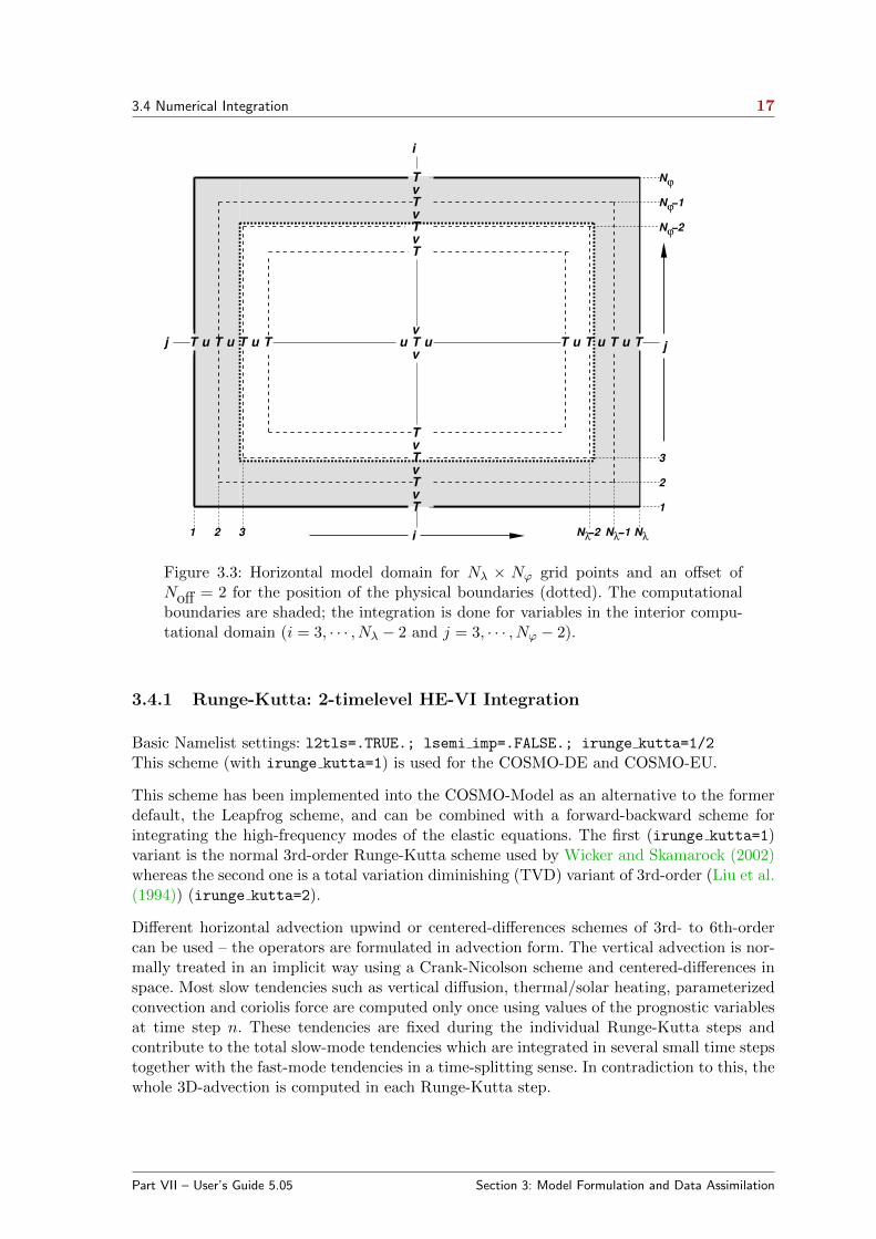
In order to implement boundary conditions and to apply the domain decomposition strategyfor code parallelization in a convenient way, the horizontal extent of the computationaldomain is chosen to be smaller than the total domain size. The lateral physical boundariesare positioned with a spatial offset from the outer boundaries to the interior. This offset is
Noff∆λ−∆λ/4 in λ-direction and
Noff∆ϕ−∆ϕ/4 in ϕ-direction,
where Noff (nboundlines as program variable) denotes the number of grid intervals used todefine the position of the physical boundaries. By default, Noff is set to 2 (larger but notsmaller numbers for Noff may be specified by the user).
All grid points interior to the physical boundary constitute the computational (or modelinterior) domain, where the model equations are integrated numerically. These are pointswith subscripts (i, j) running from i = Noff+1, · · · , Nλ−Noff and j = Noff+1, · · · , Nϕ−Noff.The extra points outside the interior domain constitute the computational boundaries. Atthese points, all model variables are defined and set to specified boundary values, but nodynamical computations are done. For Noff = 2, we have two extra lines of grid pointsadjacent to each physical boundary (see Fig. 3.3).
3.4 Numerical Integration
Because the governing nonhydrostatic equations describe a compressible model atmosphere,meteorologically unimportant sound waves are also part of the solution. As acoustic waves arevery fast, their presence severely limits the time step of explicit time integration schemes. Inorder to improve the numerical efficiency, the prognostic equations are separated into termswhich are directly related to acoustic and gravity wave modes and into terms which refer tocomparatively slowly varying modes of motion. This mode-splitting can formally be writtenin the symbolic form
∂ψ
∂t= sψ + fψ , (3.12)
where ψ denotes a prognostic model variable, fψ the forcing terms due to the slow modesand sψ the source terms related to the acoustic and gravity wave modes. sψ is made upof the pressure gradient terms in the momentum equations, the temperature and pressurecontributions to the buoyancy term in the w-equation and the divergence term in the pres-sure and the temperature equation. The subset of equations containing the sψ-terms is thenintegrated with a special numerical scheme. The COSMO-Model provides four different in-tegration methods.
Part VII – User’s Guide 5.05 Section 3: Model Formulation and Data Assimilation
3.4 Numerical Integration 17
TT T Tu u u T T T Tu u u
T
T
T
T
v
v
v
T
T
T
T
v
v
v
Tv
vuu
1 2 3
1
2
3
N
N
N
N
λNλ−1N −2λ
ϕ
ϕ
ϕ
−1
−2
i
jj
i
Figure 3.3: Horizontal model domain for Nλ × Nϕ grid points and an offset ofNoff = 2 for the position of the physical boundaries (dotted). The computationalboundaries are shaded; the integration is done for variables in the interior compu-tational domain (i = 3, · · · , Nλ − 2 and j = 3, · · · , Nϕ − 2).
3.4.1 Runge-Kutta: 2-timelevel HE-VI Integration
Basic Namelist settings: l2tls=.TRUE.; lsemi imp=.FALSE.; irunge kutta=1/2
This scheme (with irunge kutta=1) is used for the COSMO-DE and COSMO-EU.
This scheme has been implemented into the COSMO-Model as an alternative to the formerdefault, the Leapfrog scheme, and can be combined with a forward-backward scheme forintegrating the high-frequency modes of the elastic equations. The first (irunge kutta=1)variant is the normal 3rd-order Runge-Kutta scheme used by Wicker and Skamarock (2002)whereas the second one is a total variation diminishing (TVD) variant of 3rd-order (Liu et al.(1994)) (irunge kutta=2).
Different horizontal advection upwind or centered-differences schemes of 3rd- to 6th-ordercan be used – the operators are formulated in advection form. The vertical advection is nor-mally treated in an implicit way using a Crank-Nicolson scheme and centered-differences inspace. Most slow tendencies such as vertical diffusion, thermal/solar heating, parameterizedconvection and coriolis force are computed only once using values of the prognostic variablesat time step n. These tendencies are fixed during the individual Runge-Kutta steps andcontribute to the total slow-mode tendencies which are integrated in several small time stepstogether with the fast-mode tendencies in a time-splitting sense. In contradiction to this, thewhole 3D-advection is computed in each Runge-Kutta step.
Part VII – User’s Guide 5.05 Section 3: Model Formulation and Data Assimilation
3.4 Numerical Integration 18
3.4.2 Leapfrog: 3-timelevel HE-VI Integration
Basic Namelist settings: l2tls=.FALSE.; lsemi imp=.FALSE.
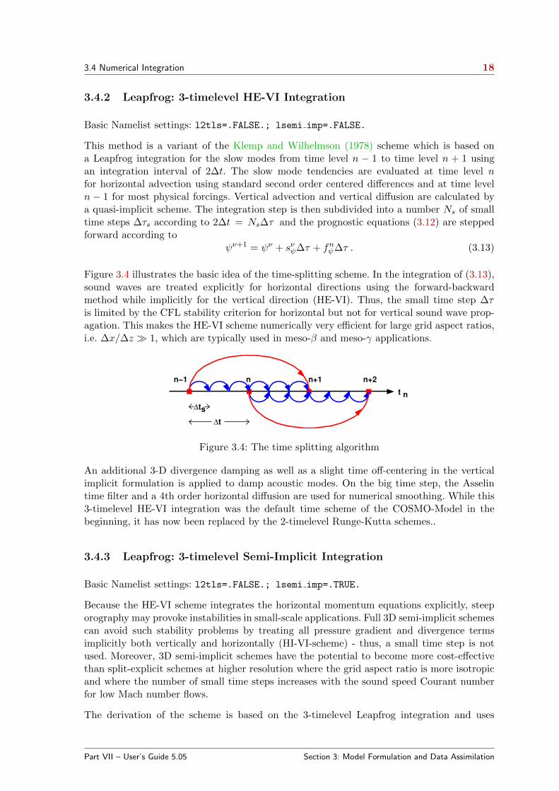
This method is a variant of the Klemp and Wilhelmson (1978) scheme which is based ona Leapfrog integration for the slow modes from time level n − 1 to time level n + 1 usingan integration interval of 2∆t. The slow mode tendencies are evaluated at time level nfor horizontal advection using standard second order centered differences and at time leveln − 1 for most physical forcings. Vertical advection and vertical diffusion are calculated bya quasi-implicit scheme. The integration step is then subdivided into a number Ns of smalltime steps ∆τs according to 2∆t = Ns∆τ and the prognostic equations (3.12) are steppedforward according to
ψν+1 = ψν + sνψ∆τ + fnψ∆τ . (3.13)
Figure 3.4 illustrates the basic idea of the time-splitting scheme. In the integration of (3.13),sound waves are treated explicitly for horizontal directions using the forward-backwardmethod while implicitly for the vertical direction (HE-VI). Thus, the small time step ∆τis limited by the CFL stability criterion for horizontal but not for vertical sound wave prop-agation. This makes the HE-VI scheme numerically very efficient for large grid aspect ratios,i.e. ∆x/∆z � 1, which are typically used in meso-β and meso-γ applications.
n−1 n n+1 n+2
t n
∆ts
∆t
Figure 3.4: The time splitting algorithm
An additional 3-D divergence damping as well as a slight time off-centering in the verticalimplicit formulation is applied to damp acoustic modes. On the big time step, the Asselintime filter and a 4th order horizontal diffusion are used for numerical smoothing. While this3-timelevel HE-VI integration was the default time scheme of the COSMO-Model in thebeginning, it has now been replaced by the 2-timelevel Runge-Kutta schemes..
3.4.3 Leapfrog: 3-timelevel Semi-Implicit Integration
Basic Namelist settings: l2tls=.FALSE.; lsemi imp=.TRUE.
Because the HE-VI scheme integrates the horizontal momentum equations explicitly, steeporography may provoke instabilities in small-scale applications. Full 3D semi-implicit schemescan avoid such stability problems by treating all pressure gradient and divergence termsimplicitly both vertically and horizontally (HI-VI-scheme) - thus, a small time step is notused. Moreover, 3D semi-implicit schemes have the potential to become more cost-effectivethan split-explicit schemes at higher resolution where the grid aspect ratio is more isotropicand where the number of small time steps increases with the sound speed Courant numberfor low Mach number flows.
The derivation of the scheme is based on the 3-timelevel Leapfrog integration and uses
Part VII – User’s Guide 5.05 Section 3: Model Formulation and Data Assimilation
3.5 Physical Parameterizations 19
the time-tendency formulation to minimize cancellation errors. An elliptic equation for thepressure perturbation tendency
L (δτ (p′) = qp
is obtained by forming the divergence of the momentum equations and eliminating the buoy-ancy terms. However, the use of a nonorthogonal curvilinear coordinate system results inan elliptic operator L containing cross-derivative terms with variable coefficients. A mini-mal residual Krylov iterative solver (GMRES) was thus chosen to solve for the perturbationpressure tendency. We found the convergence criterion proposed by Skamarock et al. (1997)to be both sufficient and a robust predictor of when the RMS divergence of the flow hasstabilized. An efficient line-Jacobi relaxation preconditioner was developed having the prop-erty that the number of Krylov solver iterations grows slowly as the convergence parameterεc decreases. Once the solution for the pressure tencendy is known, the other variables areupdated by back-substitution.
3.5 Physical Parameterizations
Some parts of the physics package of the COSMO-Model are adapted from the former oper-ational hydrostatic model DM. Others have been widely rewritten or were replaced by newdevelopments. This section gives a short overview on the parameterization schemes used. Adetailed description is given in Part II of the Documentation, Physical Parameterizations.
3.5.1 Radiation
Basic Namelist settings: lphys=.TRUE.; lrad=.TRUE.; hincrad=1.0
To calculate the heating rate due to radiation we employ the parameterization scheme ofRitter and Geleyn (1992). This scheme is based on a δ-two-stream version of the generalequation for radiative transfer and considers three shortwave (solar) and five longwave (ther-mal) spectral intervals. Clouds, aerosol, water vapour and other gaseous tracers are treatedas optically active constituents of the atmosphere, which modify the radiative fluxes byabsorption, emission and scattering.
As an extension to the original scheme, a new treatment of the optical properties of ice par-ticles has been introduced which allows a direct cloud-radiative feedback with the predictedice water content when using the cloud ice scheme for the parameterization of cloud andprecipitation.
Numerically, the parameterization scheme is very cost-intensive. Thus, it is called only athourly intervals during an operational forecast on the meso-β scale. The resulting short-and longwave heating rates are then stored and remain fixed for the following time interval.In case of high resolution simulations, the calling frequency of the radiation scheme can beincreased to allow for a better representation of the interaction with the cloud field. Theradiation can also be computed on a coarser grid to save computation time.
3.5.2 Grid-scale Precipitation
Basic Namelist settings: lphys=.TRUE.; lgsp=.TRUE.
Part VII – User’s Guide 5.05 Section 3: Model Formulation and Data Assimilation

3.5 Physical Parameterizations 20
The basic parameterization scheme for the formation of grid-scale clouds and precipitationis an adapted version of the DM-scheme. It is based on a Kessler-type bulk formulation anduses a specific grouping of various cloud and precipitation particles into broad categories ofwater substance. The particles in these categories interact by various microphysical processeswhich in turn have feedbacks with the overall thermodynamics. Microphysical processes areparameterized by corresponding mass transfer rates between the categories and are formu-lated in terms of the mixing ratios as the dependent model variables.
Besides water vapour in the gaseous phase three categories of water are considered by thedefault scheme:
- cloud water is in the form of small suspended liquid-phase drops. Cloud droplets aresmaller than about 50 µm in radius and thus have no appreciable terminal fall speedrelative to the airflow.
- rain water is in the form of liquid-phase spherical drops which are large enough tohave a non-negligible fall velocity. An exponential Marshall-Palmer size-distributionis assumed for the raindrops and a drop terminal velocity depending only on dropdiameter is prescribed.
- Snow is made up of large rimed ice particles and rimed aggregates which are treatedas thin plates with a specific size-mass relation. Particles in this category have a non-negligible terminal velocity which is prescribed to depend only on particle size. Anexponential Gunn-Marshall size-distribution is assumed.
The budget equation for the specific water contents q of the various categories (water vapourqv, cloud water qc, cloud ice qi and graupel qg, depending on the scheme used) take advectiveand turbulent transport into account and contain source and sink terms due to the micro-physical processes of cloud and precipitation formation. For rain water qr and snow qs, onlyadvective transport is considered. The following mass-transfer rates are considered by thescheme:
(a) condensation and evaporation of cloud water,
(b) the initial formation of rainwater by autoconversion and of snow by nucleation fromthe cloud water phase,
(c) the subsequent growth of the precipitation phases rain and snow by accretion, riming,deposition and shedding,
(d) evaporation of rainwater and sublimation of snow in subcloud layers and
(e) melting of snow to form rain and freezing of rain to form snow.
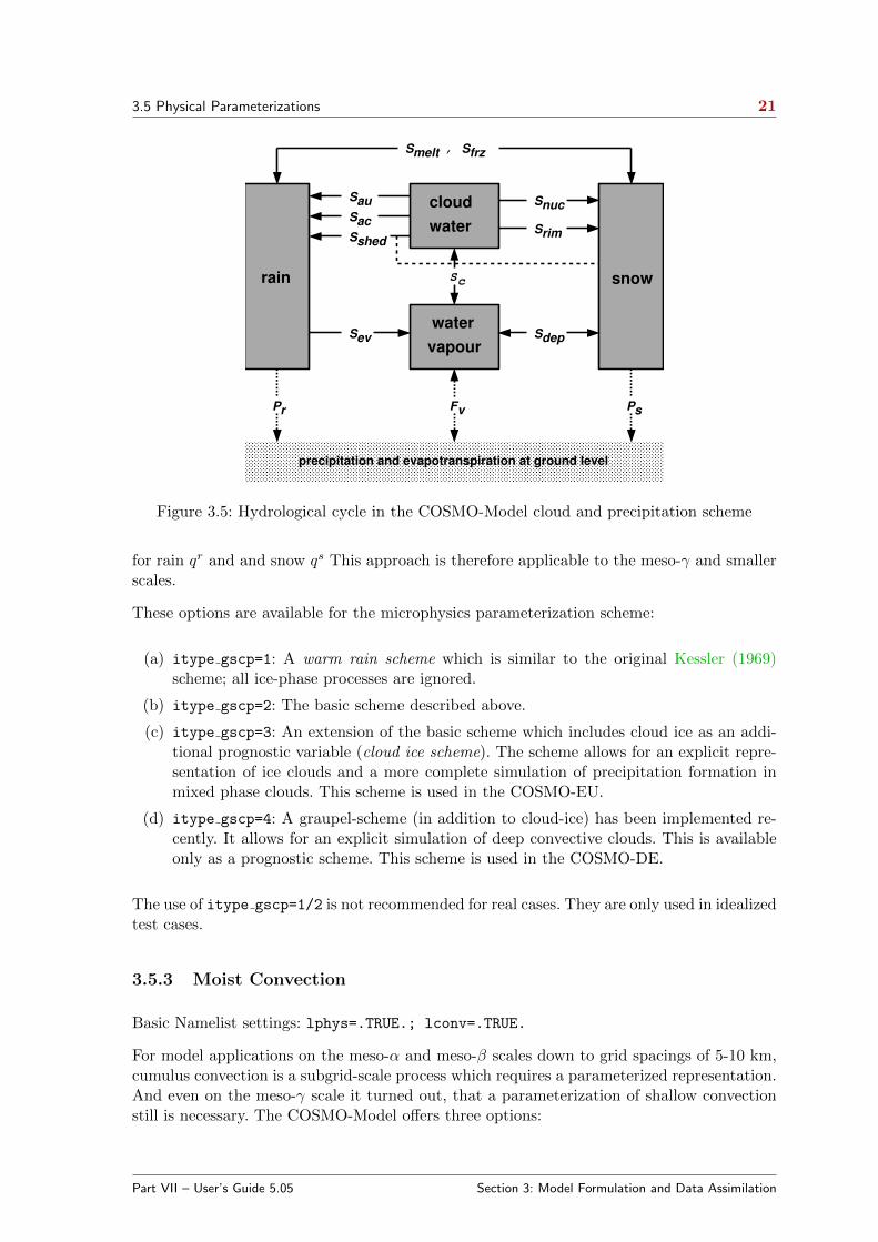
The impact of the vertical motion of rain and snow relative to the airflow due to the sedi-mentation of particles with their terminal velocities is also taken into account by the verticaldivergence of the corresponding precipitation fluxes Pr and Ps. Figure 3.5 illustrates themicrophysical processes considered by this parameterization scheme.
In contrast to the former diagnostic precipitation scheme with its assumption of columnequilibrium for the precipitating particles, we now solve the complete prognostic equations
Part VII – User’s Guide 5.05 Section 3: Model Formulation and Data Assimilation
3.5 Physical Parameterizations 21
au
S
S
ac
shed
Sev
S
S
S
nuc
rim
dep
Smelt , Sfrz
S
Sc
FvPr Ps
CCCCCCCCCCCCCCCCCCCCCCCCCCCCCCCCCCCCCCCCCCCCCCCCCCCCCCCCCCCCCCCCCCCCCCCCCCCCCCCCCCCCCCCCCCCCCCCCCCCCCCCCCCCCCCCCCCCCCCCCCCCCCCCC
rain
water
vapour
cloud
water
precipitation and evapotranspiration at ground level
snow
Figure 3.5: Hydrological cycle in the COSMO-Model cloud and precipitation scheme
for rain qr and and snow qs This approach is therefore applicable to the meso-γ and smallerscales.
These options are available for the microphysics parameterization scheme:
(a) itype gscp=1: A warm rain scheme which is similar to the original Kessler (1969)scheme; all ice-phase processes are ignored.
(b) itype gscp=2: The basic scheme described above.
(c) itype gscp=3: An extension of the basic scheme which includes cloud ice as an addi-tional prognostic variable (cloud ice scheme). The scheme allows for an explicit repre-sentation of ice clouds and a more complete simulation of precipitation formation inmixed phase clouds. This scheme is used in the COSMO-EU.
(d) itype gscp=4: A graupel-scheme (in addition to cloud-ice) has been implemented re-cently. It allows for an explicit simulation of deep convective clouds. This is availableonly as a prognostic scheme. This scheme is used in the COSMO-DE.
The use of itype gscp=1/2 is not recommended for real cases. They are only used in idealizedtest cases.
3.5.3 Moist Convection
Basic Namelist settings: lphys=.TRUE.; lconv=.TRUE.
For model applications on the meso-α and meso-β scales down to grid spacings of 5-10 km,cumulus convection is a subgrid-scale process which requires a parameterized representation.And even on the meso-γ scale it turned out, that a parameterization of shallow convectionstill is necessary. The COSMO-Model offers three options:
Part VII – User’s Guide 5.05 Section 3: Model Formulation and Data Assimilation

3.5 Physical Parameterizations 22
(a) Mass flux Tiedtke schemeBasic Namelist settings: itype conv=0
The mass flux scheme of Tiedtke (1989), which is used in coarser grid applications(above 3 km), has been implemented for the meso-α and meso-β scale. This parame-terization discriminates three types of moist convection: shallow convection, penetrativeconvection and midlevel convection, which are treated by different closure conditions.Both shallow and penetrative convection have their roots in the atmospheric boundarylayer but they differ in vertical extent. Midlevel convection, on the other hand, has itsroots not in the boundary layer but originates at levels within the free atmosphere.
As a closure condition, the Tiedtke scheme requires a formulation of the vertical massflux at the convective cloud base in terms of the grid-scale variables. For shallow andpenetrative convection, it is assumed that this mass flux is proportional to the verticallyintegrated moisture convergence between the surface and the cloud base. In case ofmidlevel convection, the mass flux is simply set proportional to the grid-scale verticalvelocity.
Given the mass flux at cloud base, the vertical redistribution of heat, moisture andmomentum as well as the formation of precipitation is then calculated by integrating asimple stationary cloud model for both updrafts and downdrafts. This finally allows tocompute the convective tendencies, i.e. the feedback of the subgrid vertical circulationonto the resolved flow. The downdrafts are assumed to originate at the level of freesinking. As an additional closure condition, the downdraft mass flux in this level isset proportional to the updraft mass flux at cloud base via a coefficient γd, which is adisposable parameter. In the present version of the scheme γd is set to a constant valueof 0.3. In subsaturated regions below cloud base, the precipitation in the downdraftsmay evaporate with a parameterized rate. Depending on the temperature of the lowestmodel layer, the precipitation is interpreted as convective snow or rain.
(b) Tiedtke-Bechtold schemeBasic Namelist settings: itype conv=2
This scheme is a modernization of the Tiedtke-scheme and is used nowadays in theECMWF IFS model. (see Bechtold et al. (2001), Bechtold et al. (2008), Bechtold et al.(2008)).
(c) A scheme for shallow convectionBasic Namelist settings: itype conv=3
This scheme has been extracted from the Tiedtke scheme and can be used for theconvection permitting scales. It is applied for the COSMO-DE.
The parameterization scheme is numerically very expensive. Thus, a timestep numberincrement can be specified for which the convection scheme is called. The convectivetendencies are then stored and remain fixed for the following time steps.
Fractional Cloud CoverIn the parameterization schemes for grid-scale clouds and precipitation the condensationrate for cloud water is based on saturation equilibrium with respect to water. Consequently,a grid element is either fully filled with clouds at water saturation where qc > 0 (relativehumidity = 100%) or it is cloud free at water subsaturation where qc = 0 (relative humidity< 100%). The area fraction of a grid element covered with grid-scale clouds is thus a bivaluedparameter which is either 1 or 0.
Part VII – User’s Guide 5.05 Section 3: Model Formulation and Data Assimilation
3.5 Physical Parameterizations 23
However, with respect to the calculation of radiative transfer but also for weather interpre-tation in postprocessing routines, it is useful to define a fractional cloud cover also for thosegrid boxes where the relative humidity is less than 100% and no grid-scale cloud water ex-ists. The calculation of the fractional cloud cover σc in each model layer is calculated basedon a traditional scheme which has been used in the former operational hydrostatic modelsEM/DM. σc is determined by an empirical function depending on the relative humidity, theheight of the model layer and the convective activity. In addition to the EM/DM scheme,the contribution of convection to σc is assumed to depend on the vertical extent of the con-vection cell by prescribing a heuristic function. Also, a check for temperature inversions atthe convective cloud tops is done to take anvils by an increase of σc in case of inversions intoaccount.
3.5.4 Vertical Turbulent Diffusion
Basic Namelist settings: lphys=.TRUE.; ltur=.TRUE.
For vertical turbulent diffusion, several schemes are available:
a) 1-D diagnostic closure:Basic Namelist settings: itype turb=1; l3dturb=.FALSE.
In the original EM/DM scheme, the vertical diffusion due to turbulent transport inthe atmosphere is parameterized by a second-order closure scheme at hierarchy level2.0 (Mellor and Yamada (1974); Muller (1981)). This results in a diagnostic closurewhere the turbulent diffusion coefficients are calculated in terms of the stability of thethermal stratification and the vertical wind shear. The impact of subgrid-scale effectson the heat and moisture fluxes due to condensation and evaporation of cloud water isnot taken into account.
b) 1-D TKE based diagnostic closure:Basic Namelist settings: itype turb=3; l3dturb=.FALSE.
For the COSMO-Model, a new scheme has been developed, which is based on a prog-nostic equation for turbulent kinetic energy (TKE), that is a level 2.5 closure scheme.The new scheme includes the transition of turbulence which contributes mainly to thefluxes (diffusive turbulence) to very small scale (dissipative) turbulence by the actionof small scale roughness elements, and the handling of non-local vertical diffusion dueto the boundary layer scale turbulence. Most important seems to be the introduc-tion of a parameterization of the pressure transport term in the TKE-equation, thataccounts for TKE-production by subgrid thermal circulations. The whole scheme isformulated in conservative thermodynamic variables together with a statistical cloudscheme according to Sommeria and Deardorff (1977) in order to consider subgrid-scalecondensation effects.
c) 3-D closure:Basic Namelist settings: itype turb=5/7; l3dturb=.TRUE.
The parameterization of subgrid-scale turbulent processes, also called a subgrid-scale(SGS) model, is of particular meaning for highly resolved LES-like model simulations.For resolutions reaching to the kilometer-scale, a more adequate turbulence param-eterization scheme should be used. For both versions described above, there is thepossibility to use a 3-D closure scheme. Up to now, this has been implemented into theCOSMO-Model only for testing purposes.
Part VII – User’s Guide 5.05 Section 3: Model Formulation and Data Assimilation
3.5 Physical Parameterizations 24
COSMO-EU and COSMO-DE use the 1-D TKE based closure scheme.
3.5.5 Parameterization of Surface Fluxes
Basic Namelist settings: lphys=.TRUE.; ltur=.TRUE.
Mesoscale numerical modelling is often very sensitive to surface fluxes of momentum, heatand moisture. These fluxes provide a coupling between the atmospheric part of the modeland the soil model. For both closure schemes described in Sec. 3.5.4, a special surface layerscheme can be applied.
a) A bulk-transfer scheme:Basic Namelist settings: itype tran=1
For the 1-D diagnostic turbulence scheme, a stability and roughness-length dependentsurface flux formulation based on Louis (1979) is implemented.
b) A TKE-based surface transfer scheme:Basic Namelist settings: itype tran=2
In context with the TKE-scheme, a revised and consistent formulation for the trans-port through the surface layer should be used. This surface scheme extends the TKE-equation to the constant flux layer and introduces an additional laminar layer justabove the surface. This makes it possible to discriminate between the values of themodel variables at the rigid surface (e.g. radiative surface temperatures) and values atthe roughness height z0 (lower boundary of the turbulent atmosphere). The Charnockformula to estimate the surface fluxes over sea is also reformulated using TKE.
COSMO-EU and COSMO-DE use the TKE based surface transfer scheme.
3.5.6 A subgrid-scale orography scheme
Basic Namelist settings: lphys=.TRUE.; lsso=.TRUE.
3.5.7 Soil Processes
Basic Namelist settings: lphys=.TRUE.; lsoil=.TRUE.
The calculation of the surface fluxes requires the knowledge of the temperature and thespecific humidity at the ground. The task of the soil model is to predict these quantitiesby the simultaneous solution of a separate set of equations which describes various thermaland hydrological processes within the soil. If vegetation is considered explicitly, additionalexchange processes between plants, ground and air have to be taken into account.
a) The (multi-layer) soil model TERRA:For land surfaces, the soil model TERRA provides the surface temperature and thespecific humidity at the ground. The ground temperature is calculated by a directsolution of the heat conduction equation and the soil water content is predicted by the
Part VII – User’s Guide 5.05 Section 3: Model Formulation and Data Assimilation
3.5 Physical Parameterizations 25
Richards equation. In the multi-layer version also the effect of freezing/melting of soilwater/ice is included and a time dependent snow albedo is introduced. Evaporationfrom bare land surfaces as well as transpiration by plants are derived as functions ofthe water content, and - only for transpiration - of radiation and ambient temperature.
Most parameters of the soil model (heat capacity, water storage capacity, etc.) stronglydepend on soil texture. Five different types are distinguished: sand, sandy loam, loam,loamy clay and clay. Three special soil types are considered additionally: ice, rock andpeat. Hydrological processes in the ground are not considered for ice and rock. Potentialevaporation, however, is assumed to occur over ice, where the soil water content remainsunchanged.
The multi-layer concept avoids the dependence of layer thicknesses on the soil type.Additionally it avoids the use of different layer structures for the thermal and thehydrological sections of the model.
Note: In COSMO-Version 5.05 the former two-/three-layer model has been eliminated.
b) The lake model FLake:Basic Namelist settings: lsoil=.TRUE.; llake=.TRUE.
FLake (Fresh-water Lake), is a lake model (parameterisation scheme) capable of pre-dicting the surface temperature in lakes of various depth on the time scales from a fewhours to many years (see http://lakemodel.net for references and other informationabout FLake). It is based on a two-layer parametric representation (assumed shape)of the evolving temperature profile and on the integral budgets of heat and kineticenergy for the layers in question. The same concept is used to describe the tempera-ture structure of the ice cover. An entrainment equation is used to compute the depthof a convectively-mixed layer, and a relaxation-type equation is used to compute thewind-mixed layer depth in stable and neutral stratification. Both mixing regimes aretreated with due regard for the volumetric character of solar radiation heating. Simplethermodynamic arguments are invoked to develop the evolution equation for the icethickness. The result is a computationally efficient bulk model that incorporates muchof the essential physics. Importantly, FLake does not require re-tuning, i.e. empiricalconstants and parameters of FLake should not be re-evaluated when the model is ap-plied to a particular lake. There are, of course, lake-specific external parameters, suchas depth to the bottom and optical properties of water, but these are not part of themodel physics.
Using the integral approach, the problem of solving partial differential equations (indepth and time) for the temperature and turbulence quantities is reduced to solvingordinary differential equations for the time-dependent quantities that specify the tem-perature profile. FLake carries the equations for the mean temperature of the watercolumn, for the mixed-layer temperature and its depth, for the temperature at the lakebottom, and for the shape factor with respect to the temperature profile in the lakethermocline (a stably stratified layer between the bottom of the mixed layer and thelake bottom). In case the lake is cover by ice, additional equations are carried for theice depth and for the ice-surface temperature. The lake-surface temperature, i.e. thequantity that communicates information between the lake and the atmosphere, is equalto either the mixed-layer temperature or, in case the lake in question is covered by ice,to the ice-surface temperature. In the present configuration (a recommended choice),the heat flux through the lake water-bottom sediment interface is set to zero and alayer of snow over the lake ice is not considered explicitly. The effect of snow above the
Part VII – User’s Guide 5.05 Section 3: Model Formulation and Data Assimilation
3.5 Physical Parameterizations 26
ice is accounted for parametrically through changes in the surface albedo with respectto solar radiation. Optionally, the bottom-sediment module and the snow module canbe switched on. Then, additional equations are carried for the snow-surface tempera-ture (temperature at the air-snow interface), for the snow depth, for the temperatureat the bottom of the upper layer of bottom sediments penetrated by the thermal wave,and for the depth of that layer. Surface fluxes of momentum and of sensible and latentheat are computed with the operational COSMO-model surface-layer parameterizationscheme. Optionally, a new surface-layer scheme can be used that accounts for specificfeatures of the surface air layer over lakes.
In order to be used within the COSMO model (or within any other NWP or climatemodel), FLake requires a number of two-dimensional external-parameter fields. Theseare, first of all, the fields of lake fraction (area fraction of a given numerical-model gridbox covered by lake water that must be compatible with the land-sea mask used) andof lake depth. Other external parameters, e.g. optical characteristics of the lake water,are assigned their default values offered by FLake. Since no tile approach is used in theCOSMO model, i.e. each COSMO-model grid box is characterised by a single land-covertype, only the grid boxes with the lake fraction in excess of 0.5 are treated as lakes.Each lake is characterised by its mean depth. Deep lakes are currently treated with thefalse bottom. That is, an artificial lake bottom is set at a depth of 50 m. The use ofsuch expedient is justified since, strictly speaking, FLake is not suitable for deep lakes(because of the assumption that the thermocline extends down to the lake bottom).However, as the deep abyssal zones typically experience no appreciable temperaturechanges, using the false bottom produces satisfactory results. A Global Land CoverCharacterization (GLCC) data set (http://edcdaac.usgs.gov/glcc) with 30 arc secresolution, that is about 1 km at the equator, is used to generate the lake-fractionfiled. The filed of lake depth is generated on the basis of a data set (developed atDWD) that contains mean depths of a number of European lakes and of major lakesof the other parts of the world. Notice that, unless tile approach is used to computethe surface fluxes, only the lake-depth external parameter filed is actually required touse FLake within the COSMO model. Setting the lake depth to its actual value for theCOSO-model grid boxes with the lake fraction in excess of 0.5, and to a negative value,say −1m, otherwise, unambiguously specifies the grid-boxes for which the lake-surfacetemperature should be computed.
c) A sea-ice scheme:Basic Namelist settings: lsoil=.TRUE., lseaice=.TRUE.
The presence of sea ice on the oceans surface has a significant impact on the air-seainteractions. Compared to an open water surface the sea ice completely changes thesurface characteristics in terms of albedo and roughness, and therefore substantiallychanges the surface radiative balance and the turbulent exchange of momentum, heatand moisture between air and sea. In order to deal with these processes the COSMOmodel includes a sea ice scheme (Mironov (2008)).
COSMO-EU and COSMO-DE use the multi-layer soil model and the FLake-Model. Thesea-ice scheme is only used in COSMO-EU.
Part VII – User’s Guide 5.05 Section 3: Model Formulation and Data Assimilation
3.6 Data Assimilation 27
3.6 Data Assimilation
Basic Namelist setting: luseobs=.TRUE.
The requirements for the data assimilation system for the operational model are mainlydetermined by the very high resolution of the model and by the task to employ it alsofor very short-range forecasting. Hence, detailed high-resolution analyses of the atmospherehave to be able to be produced frequently, and this requires a thorough use of asynopticand high-frequency observations such as aircraft data and remote sensing data. Note thatthe synoptic scales are largely determined by the lateral boundary conditions provided bythe driving model, and the main purpose of the assimilation scheme is to analyze the mesoscales.
By design, 3-dimensional analysis methods tend to be less appropriate for this purpose. Theydo not allow to account for the exact observation time of asynoptic data, and they makeit necessary to neglect most of the high-frequent data unless the analysis scheme is appliedvery frequently at significant computational costs. Moreover, the geostrophic approximation,a key ingredient of some of these schemes as used e.g. for the GME, is of limited validityon the meso scale. Therefore, 4-dimensional methods offer potential advantages since theyinclude the model dynamics in the assimilation process directly. However, the 4-dimensionalvariational (4DVAR) method has been too expensive in the past for operational applicationconsidering the small amount of time available to produce the analyses and forecasts.
a) Observation Nudging —— Basic Namelist setting: lnudge=.TRUE.
Therefore, a scheme based on the observation nudging technique has been developedto define the atmospheric fields. It is based on an experimental nudging assimilationscheme which had been developed for the former hydrostatic model DM and its Swissversion SM (Schraff (1996); Schraff (1997)) and which compared favorably with theat that time operational Optimum Interpolation analysis of DM in a number of testcases. The scheme for COSMO has then been adapted to the nonhydrostatic modellingframework and runs on distributed memory machines using domain decomposition.
Nudging or Newtonian relaxation consists of relaxing the prognostic model variablestowards prescribed values within a predetermined time window (see e.g. Davies andTurner (1977); Stauffer and Seaman (1990)). In the present scheme, nudging is per-formed towards direct observations which is more appropriate for high-resolution ap-plications than nudging towards 3-dimensional analyses (Stauffer and Seaman (1994)).A relaxation term is introduced into the model equations, and the tendency for aprognostic variable ψ(x, t) is given by
∂
∂tψ(x, t) = F (ψ,ψ x, t) + Gψ ·
∑k(obs)
Wk · [ψk − ψ(xk, t)] (3.14)
F denotes the model dynamics and physical parameterizations, ψk the value of the kth
observation influencing the grid point x at time t, xk the observation location, Gψ theconstant so-called nudging coefficient, and Wk an observation-dependent weight whichusually varies between 0 and 1. Neglecting the dynamics and physics and assuming asingle observation with a constant weight Wk equal 1, the model value at the observa-tion location relaxes exponentially towards the observed value with an e-folding decayrate of 1/Gψ corresponding to about half an hour. The observational information is
Part VII – User’s Guide 5.05 Section 3: Model Formulation and Data Assimilation
3.6 Data Assimilation 28
provided to the nudging scheme in the form of NetCDF observation input files whichare described in Section 5.4.
In practical applications, the nudging term usually remains smaller than the largestterm of the dynamics so that the dynamic balance of the model is not strongly dis-turbed. The coupling between the mass and wind field innovations is primarily inducedimplicitly by the model dynamics. If the assimilation process is successful the modelfields will be close to dynamic balance at the beginning of the forecast, and an initial-ization step is not required.
b) Latent Heat Nudging —— Basic Namelist setting: llhn=.TRUE.
Radar-derived precipitation rates can be assimilated by an extra Latent Heat Nudgingscheme (Stephan et al. (2008)). It computes additional temperature and humidityincrements at each model column independently from each other. It is tuned and shouldbe used only for convection-permitting model configurations (with horizontal meshwidths of ≤ 3 km). The observation input is gridded precipitation rates read in theform of extra Grib files. Further Grib files can be read optionally, containing a blacklist,and radar beam height maps utilised for bright band detection.
c) Analysis of surface and soil fields, outside COSMO code
In addition to the nudging-type assimilation schemes for the atmosphere, a set of 2-dimensional intermittent analysis schemes can be applied for some of the surface andsoil fields in a full data assimilation cycle for the COSMO model. This comprises ofa variational soil moisture analysis (Hess (2001)), a snow analysis, and a sea surfacetemperature (SST) analysis (including an analysis of sea ice cover). These analysisschemes are not integrated into the COSMO code, but are programs on their own.Therefore, they are not covered by this User’s Guide, even though a scientific descrip-tion or outline of them is included in the COSMO Documentation Part III on dataassimilation.
d) Diagnostic surface analyses —— Basic Namelist setting: lsurfa=.TRUE.
In contrast, the data assimilation code of the COSMO model includes a module witha Cressman-type successive correction analysis scheme, which can be used to computea set of other 2-dimensional surface-level analyses. This set comprises of a 2-m tem-perature, 2-m relative humidity, 10-m wind speed, and surface precipitation analysis.While the precipitation analysis is purely based on rain gauge (surface synoptic) data,the other analyses use the corresponding model field as a first guess purely to helpdefining the small-scale details that are not resolved by the surface observations. Allthese analyses are used only for diagnostic purposes. As an exception, the daytime2-m temperature and optionally 2-m humidity analyses are used in the variational soilmoisture analysis.
Part VII – User’s Guide 5.05 Section 3: Model Formulation and Data Assimilation
29
Section 4
Installation of the COSMO-Model
This chapter explains the steps necessary to compile and run the model. Section 4.1 lists theexternal libraries that are necessary to run different components of the model and what canbe done, if these libraries are not available. The next sections give detailed informations onhow to prepare, compile, link and run the COSMO-Model.
4.1 External Libraries for the COSMO-Model
For some components, the COSMO-Model uses external libraries. Usage of most of theselibraries can be controlled by conditional compilation. To handle this, the C preprocessor(cpp) must be called. Most Fortran compilers activate the C preprocessor for files endingwith a capital F in the suffix: .F or .F90. The COSMO-Model does not use capital lettersin the suffix, therefore a special compiler option has to be set, to activate this preprocessor.Take a look to the manual of your compiler to find out about this option.
4.1.1 libgrib1.a:
The original implementation of INT2LM and the COSMO-Model used GRIB (Grided Bi-nary), Version 1, as standard format. Coding and decoding of GRIB1 records can be donewith the DWD GRIB1 library, the libgrib1.a. This library also contains C-routines towrite data to and read it from disk. The Grib library is available from DWD and is providedtogether with the source code for the COSMO-Model. A short guide for the installation isincluded in the tar-file of the Grib library.
With GRIB1, DWD used a Grib file format, where all records are starting and ending withadditional bytes, the so-called controlwords. To process these controlwords properly, you haveto set the environment variable
export LIBDWD FORCE CONTROLWORDS=1
Usage of the DWD GRIB1 library can be controlled by conditional compilation and settingthe macro GRIBDWD. If this macro is not set during compilation, the parts of the source code
Part VII – User’s Guide 5.05 Section 4: Installation of the COSMO-Model

4.1 External Libraries for the COSMO-Model 30
that do use libgrib1.a calls are not compiled and the library will not be linked to thebinary.
4.1.2 libgrib api.a, libgrib api f90.a:
Since Version 4.28 another grib library can be used to read grib data. This is the grib api
(Application Programmer’s Interface) from ECMWF. With this library it is possible toread and write also GRIB2 data (i.e. GRIB, Version 2). grib api will be replaced soonby ecCodes, which contains grib api and a bufr-library. Source codes for both librariestogether with installation instructions are available from the ECMWF web pages:http://www.ecmwf.int/en/computing/software.
To use grib api properly, two sets of definition files are necessary for running the programs:one contains all original definitions from ECMWF (definitions), the other set is com-piled and maintained by DWD and must be used for the INT2LM and the COSMO-Model(definitions.edzw). Also, some special sample files are needed by both programs.
Both sets of definition files and the necessary samples, which have to correspond to thegrib api version used, are distributed together with the INT2LM by DWD. For INT2LMand the COSMO-Model, at least grib api Version 1.11.0 or higher is required to read GRIB2data. For writing GRIB2 data, at least grib api Version 1.13.1 is required. At DWD we usegrib api-1.20.0 with COSMO Version 5.05.
Please read more on grib api and its usage in the Documentation, Part VI, Model Outputand Data Formats for I/O.
Usage of the grib api library can be controlled by conditional compilation and setting themacro GRIBAPI. If this macro is not set during compilation, the parts of the source code thatdo use grib api calls are not compiled and the library will not be linked to the binary.
4.1.3 libnetcdf.a:
Since Version 3.18, input and output of data can also be done in the NetCDF format (Net-work Common Data Format). Using NetCDF requires an external library libnetcdf.a. Thesource code of this library can be downloaded from http://www.unidata.ucar.edu .
Usage of the NetCDF library can be controlled by conditional compilation and setting themacro NETCDF. If this macro is not set during compilation, the parts of the source code thatdo use NetCDF calls are not compiled and the library will not be linked to the binary.
NOTE:The usage of NetCDF can only be avoided, if also the Nudging is switched off. If Nudging(the data assimilation) shall be used, a NetCDF library has to be available, because theobservation processing is done via NetCDF.
4.1.4 libmisc.a:
Before Version 4.24 of the COSMO-Model, a library libmisc.a was needed for special appli-cations in the data assimilation (the nudging). Since version 4.24 this library is not necessary
Part VII – User’s Guide 5.05 Section 4: Installation of the COSMO-Model

4.1 External Libraries for the COSMO-Model 31
any more.
4.1.5 libcsobank.a, libsupplement.a:
Before COSMO-Model 4.25 and INT2LM 2.1
The COSMO-Model and INT2LM use a tool for parallel asynchronous I/O from or to filesor a data base system (only for Grib). The routines for that tool are grouped together in amodule mpe io.f90. In the VCS of DWD, mpe io.f90 is provided as an external module,hence it is not in the source code of the model library. mpe io.f90 uses the two librarieslibcsobank.a and libsupplement.a.
For users outside DWD, mpe io.f90 has been included in the source code of the COSMO-Model and also in the INT2LM. To satisfy the calls from mpe io to the data base system,an additional file dummy db.f90 is provided.
• NEW:Since COSMO-Model Version 4.25 and INT2LM Version 2.1, mpe io.f90 has beenreplaced by a modified version mpe io2.f90, which does not support the databaseaccess any more. Therefore the usage of these external libraries is now obsolete.
4.1.6 libRTTOVxx.a:
Since Version 3.7 the COSMO-Model contains an interface to the RTTOV7-library (Radia-tive Transfer Model). This interface has been developed at the DLR Institute for AtmosphericPhysics in Oberpfaffenhofen. Together with the RTTOV7-library it is possible to computesynthetic satellite images (brightness temperatures and radiances) derived from model vari-ables for Meteosat5-7 and Meteosat Second Generation.
In subsequent versions also newer RTTOV libraries can be used:
• Between Versions 4.18 and 5.04e: RTTOV9
• Since Version 4.26: RTTOV10
• Since Version 5.05: RTTOV12
The RTTOV model has been developed by UKMO et.al. in the framework of the ESA NWP-SAF. To use any version of the RTTOV model, a license is necessary. For getting this license,please contact [email protected].
Usage of the RTTOV libraries can be controlled by conditional compilation and settingone of the macros RTTOVxx, with x ∈ {7, 910, 12}. Note that RTTOV7 has been modified atDWD to be used in parallel programs. For the usage of RTTOV9, RTTOV10 and RTTOV12,a special interface mo rttov ifc.f90 is necessary, which can also be obtained from DWDtogether with installation instructions.
If the license (and hence the RTTOV libraries) is not available, the corresponding macrosmust not be set. The computation of the synthetic satellite images is not possible then.
Part VII – User’s Guide 5.05 Section 4: Installation of the COSMO-Model
4.2 Preparing the Code 32
4.2 Preparing the Code
You have got a tar-file cosmo yymmdd x.y, where yymmdd describes the date in the form”Year-Month-Day” and x.y gives the version number. By de-taring, a directory is createdwith the following contents:
DOCS Contains a short documentation of the changes in version x.
edid Script to edit files in src and store them in work.
Fopts Definition of the compiler options and also directories of libraries.
LOCAL Contains several examples of Fopts-files for different computers.
Makefile For compiling and linking the programs.
RUNSCRIPTS Several examples of scripts (run cosmo xx or run ideal xx) toset the Namelist values for a configuration xx or for idealized testcases and start the program.
src Subdirectory for the source code.
obj Subdirectory where the object files are written.
ObjDependencies Definition of the dependencies between the different source files.
Objfiles Definition of the object files.
work Subdirectory for intermediate files.
The directories ./obj and ./work are empty and can therefore get lost by the tar-process.If so, you have to create them again. In edid you have to adapt the pathnames if you wantto work with it.
4.3 Compiling and Linking
You have to choose the options for compiling the code in Fopts. See the User Guide of yourcomputer system for necessary and/or desired options. In particular you have to set themacros to select external libraries. Since COSMO-Model Version 5.1 you definitely have toset the macro -D COSMO ! Before linking check that all necessary external libraries (see 4.1)are available.
Before compiling and linking the program you have to decide whether you want to run insingle or in double precision. When running in single precision the usage of data assimilationand RTTOV libraries is not possible yet. If you want to run in single precision, you have todefine the macro -DSINGLEPRECSION in the Fopts-file. If you do not specify this macro, thedefault is to run the COSMO-Model in double precision.
All other input variables for the program can be determined before running the programwith the NAMELIST-input (see Chapter 6).
The COSMO-Model is parallelized for distributed memory parallel computers using thedomain decomposition technique and explicit message passing with the Message PassingInterface (MPI). Thus it can run on parallel platforms but also on sequential platformswhere MPI is not available. For this purpose an additional module dummy mpi.f90, togetherwith a file mpif.h, are provided in the directory LOCAL. Place these files in the src-directorybefore compiling and linking. Then you can only create sequential binaries (see below).
Part VII – User’s Guide 5.05 Section 4: Installation of the COSMO-Model
4.4 Running the Code 33
You can invoke a make-run by typing make entry. The following entries are available. Notethat the special entry has to correspond to the settings of the macros. seq or par correspondto the sequential or parallel mode, resp.
pur[par|seq] A pure binary without nudging and synthetic satellite images. -DNUDGING,-DRTTOVx and -DNETCDF must not be set.
all[par|seq] A full binary with nudging and synthetic satellite images, if -DNUDGING,-DNETCDF and -DRTTOVx are set.
nud[par|seq] A binary with nudging but without synthetic satellite images. -DNUDGINGand -DNETCDF must be set and -DRTTOVx must not be set.
sat[par|seq] A binary without nudging but with synthetic satellite images. -DNUDGINGmust not be set and -DRTTOVx must be set.
More entries can be added on your own.
4.4 Running the Code
To run the code, several ASCII-files INPUT *** have to be provided that contain values forthe NAMELIST variables. The form of these INPUT *** files is described in Chapters 5 and 6.They are created by the provided run-scripts.
The run-scripts also contain the command to invoke the binary, which you have to adapt.While a sequential binary usually can be invoked just by typing <name of binary>, a parallelbinary must be invoked by a special tool. Often this tool is mpirun, but also other tools arepossible. See the manual for your system on how to invoke the binary created in the laststep.
Part VII – User’s Guide 5.05 Section 4: Installation of the COSMO-Model
34
Section 5
Input Files for the COSMO-Model
The COSMO-Model requires several input files.
- ASCII-files, called INPUT *** (see below for the exact filenames), that contain thenamelist variables. The form of these files is described in Section 5.1. The namelistgroups, the variables, their meanings and possible values are described in Chapter 6for the model and in Chapter 7 for the data assimilation.
- GRIB-Code or NetCDF files for the initial and boundary values. These files are de-scribed in Section 5.2 and in Section 5.3, respectively. Please note that there is a shortdescription of the GRIB and NetCDF data formats now available in the Part VI of themodel documentation.
- NetCDF observation input files which contain the observational information for dataassimilation (nudging) and for producing a NetCDF feedobs file. The purpose of thefeedobs file is to serve as input to a LETKF analysis scheme or to verification tools.The NetCDF observation input files, including a blacklist file, are described in Section5.4.
5.1 Files for Namelist Input
The COSMO-Model uses NAMELIST-input to specify runtime parameters. The parametersare splitted into several groups, which are distributed to the components. Table 5.1 lists thecomponents, the groups and the corresponding INPUT *** files.
The last group of component Input / Output (GRIBOUT) can occur several times. Every groupcan determine a different list of variables for output and also different output steps.
The program provides default values for all parameters. To change a default value, an appro-priate NAMELIST statement has to appear in the corresponding ASCII-file INPUT ***. Theform of a NAMELIST statement depends on the specific platform you are using but is alwayssimilar to the following (refer to the Language Reference Manual of your system):
1. The ampersand (&) character, followed immediately by the name of the namelist group.
Part VII – User’s Guide 5.05 Section 5: Input Files for the COSMO-Model
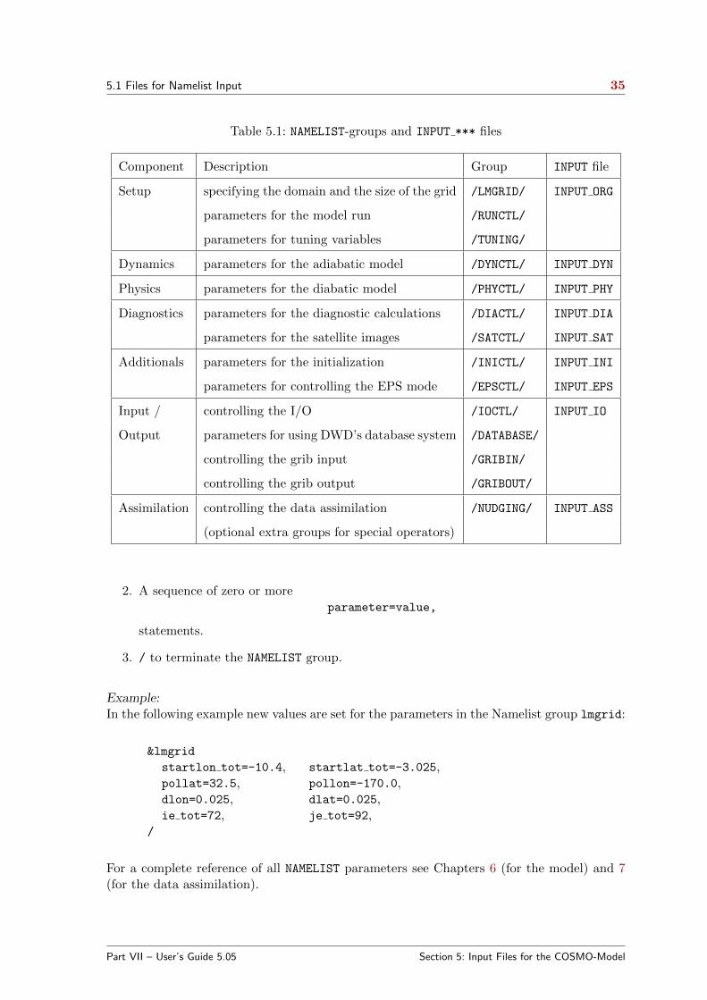
5.1 Files for Namelist Input 35
Table 5.1: NAMELIST-groups and INPUT *** files
Component Description Group INPUT file
Setup specifying the domain and the size of the grid /LMGRID/ INPUT ORG
parameters for the model run /RUNCTL/
parameters for tuning variables /TUNING/
Dynamics parameters for the adiabatic model /DYNCTL/ INPUT DYN
Physics parameters for the diabatic model /PHYCTL/ INPUT PHY
Diagnostics parameters for the diagnostic calculations /DIACTL/ INPUT DIA
parameters for the satellite images /SATCTL/ INPUT SAT
Additionals parameters for the initialization /INICTL/ INPUT INI
parameters for controlling the EPS mode /EPSCTL/ INPUT EPS
Input / controlling the I/O /IOCTL/ INPUT IO
Output parameters for using DWD’s database system /DATABASE/
controlling the grib input /GRIBIN/
controlling the grib output /GRIBOUT/
Assimilation controlling the data assimilation /NUDGING/ INPUT ASS
(optional extra groups for special operators)
2. A sequence of zero or moreparameter=value,
statements.
3. / to terminate the NAMELIST group.
Example:In the following example new values are set for the parameters in the Namelist group lmgrid:
&lmgrid
startlon tot=-10.4, startlat tot=-3.025,pollat=32.5, pollon=-170.0,dlon=0.025, dlat=0.025,ie tot=72, je tot=92,
/
For a complete reference of all NAMELIST parameters see Chapters 6 (for the model) and 7(for the data assimilation).
Part VII – User’s Guide 5.05 Section 5: Input Files for the COSMO-Model

5.2 Conventions for File Names 36
5.2 Conventions for File Names
The initial and boundary fields needed for the model are provided either in Grib or inNetCDF format. Also for the output files, one can choose between Grib or NetCDF. Restartfiles are written in binary format with full precision. There is one file for the initial fieldsand also for every set of boundary fields. The following conventions apply for the filenames.
A file name for the COSMO-Model or the INT2LM has the general form
yheader // ydate // yextension (for Grib files),or
yheader // ydate // yextension // ’.nc’ (for NetCDF files),
where yheader, ydate and yextension have the following meaning:
yheader: File header (3 characters, only for ICON 4 characters)
- first character: specifies the model
ig: ICON (global model)
g: GME (global model)
l: COSMO-Model
e: ECMWF model IFS (Integrated Forecast System)
c: A general (global) climate model
- second character (for ICON: third character):
a: analysis file (uninitialized)
i: analysis file (initialized)
b: boundary file
f: forecast files
r: restart files
- third character (for ICON fourth character): specifies the region covered by the data
f: full model domain
s: subdomain
ydate: There are two forms of specifying the date, either with the full date or relative to thestart date:
- In the name of analysis files (second character in the header a or i) the full date isspecified: ydate = ’yyyymmddhh’ with yyyy: year; mm: month; dd: day; hh: hour.
Example:
laf1992072100 COSMO-Model, uninitialized analysis for full model domainfrom July, 21st, 1992.
Part VII – User’s Guide 5.05 Section 5: Input Files for the COSMO-Model

5.2 Conventions for File Names 37
Since COSMO-Model Version 4.24, the initial date can be specified with 14 digits,where the last digits represent minutes and seconds. If the namelist variable ydate ini
is specified with 14 digits, also for the filenames 14 digits are used.
- In forecast, boundary or restart files, ydate consists of a single character (the time unitof forecast range, ytunit), followed by a string.
ydate = ytunit // ’string’
Depending on ytunit, the string has the following meaning:
t: timestep mode: forecast range given in timesteps
f: forecast mode: the forecast range is given in the form ddhhmmss, where dd: day,hh: hour, mm: minute, ss: second
c: climate mode: the forecast range is given in the form yyydddhh, where yyy: year,ddd: day of the year, hh: hour
d: day mode: the full date is given in the form ’yyyymmddhh’, where yyyy: year; mm:month; dd: day; hh: hour
yextension (1 character, optional): Extension, e.g. data interpolated from model to pressurelevels.
Examples:
lbff00050000 COSMO-Model, file with boundary values for hour 5lfff01233000 COSMO-Model, forecast at day 1, 23 hours and 30 minutes.lrff01000000 COSMO-Model, restart file for day 1.
Part VII – User’s Guide 5.05 Section 5: Input Files for the COSMO-Model
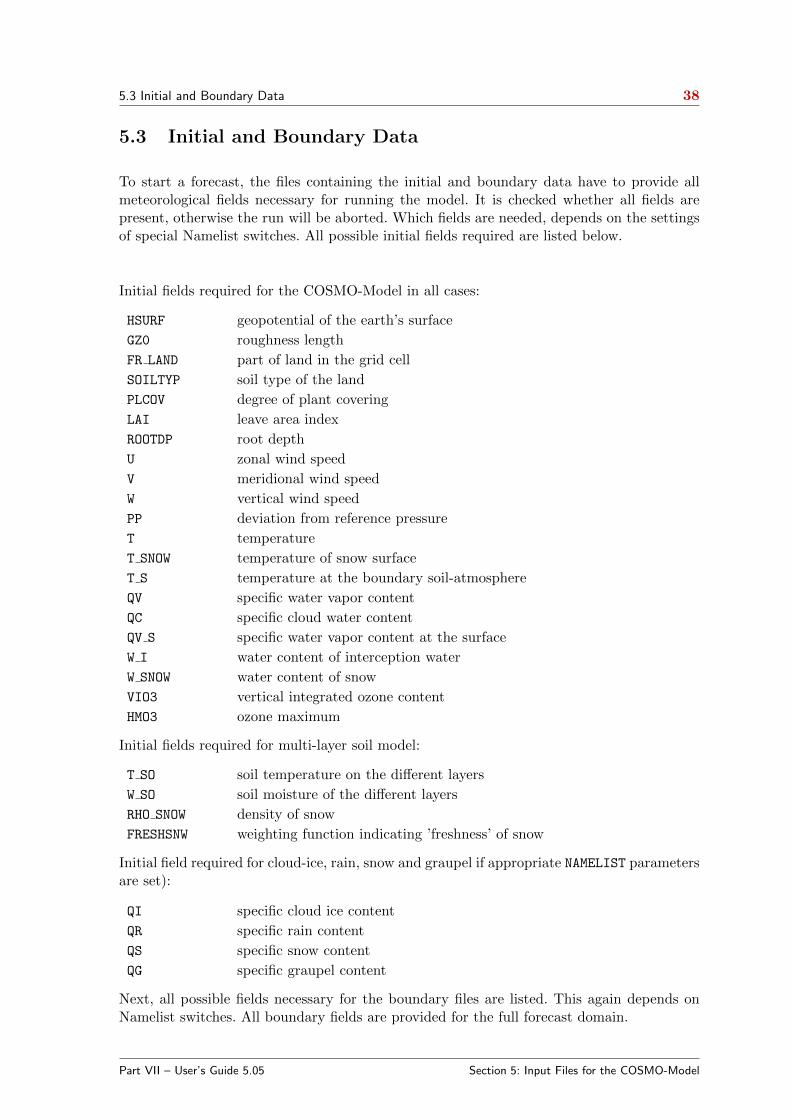
5.3 Initial and Boundary Data 38
5.3 Initial and Boundary Data
To start a forecast, the files containing the initial and boundary data have to provide allmeteorological fields necessary for running the model. It is checked whether all fields arepresent, otherwise the run will be aborted. Which fields are needed, depends on the settingsof special Namelist switches. All possible initial fields required are listed below.
Initial fields required for the COSMO-Model in all cases:
HSURF geopotential of the earth’s surface
GZ0 roughness length
FR LAND part of land in the grid cell
SOILTYP soil type of the land
PLCOV degree of plant covering
LAI leave area index
ROOTDP root depth
U zonal wind speed
V meridional wind speed
W vertical wind speed
PP deviation from reference pressure
T temperature
T SNOW temperature of snow surface
T S temperature at the boundary soil-atmosphere
QV specific water vapor content
QC specific cloud water content
QV S specific water vapor content at the surface
W I water content of interception water
W SNOW water content of snow
VIO3 vertical integrated ozone content
HMO3 ozone maximum
Initial fields required for multi-layer soil model:
T SO soil temperature on the different layers
W SO soil moisture of the different layers
RHO SNOW density of snow
FRESHSNW weighting function indicating ’freshness’ of snow
Initial field required for cloud-ice, rain, snow and graupel if appropriate NAMELIST parametersare set):
QI specific cloud ice content
QR specific rain content
QS specific snow content
QG specific graupel content
Next, all possible fields necessary for the boundary files are listed. This again depends onNamelist switches. All boundary fields are provided for the full forecast domain.
Part VII – User’s Guide 5.05 Section 5: Input Files for the COSMO-Model

5.3 Initial and Boundary Data 39
Boundary fields required for the COSMO-Model:
U BD zonal wind speed
V BD meridional wind speed
PP BD deviation from reference pressure
T BD temperature
T snow BD temperature of snow surface
QV BD specific water vapor content
QC BD specific cloud water content
QV S BD specific water vapor content on the surface
W SNOW BD water content of snow
For the multi-layer soil model, no boundary fields are necessary. If the model should runwith cloud-ice, also the following field is needed.
Boundary field required for cloud-ice, rain and snow if appropriate NAMELIST parameters areset):
QI specific cloud ice content
QR specific rain content
QS specific snow content
If the NAMELIST parameter lartif data is set to .TRUE. (see 6.2), the input of initialand boundary data is skipped and artificial data are generated instead in the routinesgen ini data and gen bound data. Note that these routines have to be edited and modifiedby the user to generate appropriate conditions for the case under consideration.
Part VII – User’s Guide 5.05 Section 5: Input Files for the COSMO-Model

5.4 Observation Input Files 40
5.4 Observation Input Files
This section describes the format of the NetCDF file observation input to the COSMOmodel and what has to be done, if these files are used as input to the nudging-type assim-ilation scheme inside COSMO, or to writing (NetCDF or ASCII (i. e. YUVERIF)) feedobsfiles for verification purposes, or to perform surface analyses based on observations (e. g. of2-m temperature). The observation input described here currently relates to conventionalobservations only, and it does not describe the (GRIB) input for the latent heat nudging.
Please note that the former alternative to read observations from the ’AOF’ files has beeneliminated in COSMO Version 5.04.
In the following items, general properties of the NetCDF file observation input aredescribed:
• Required files and file names:
The NetCDF observation input files have fixed file names which are given in the fol-lowing sub-sections and begin with ’cdfin ’. For the observation file type ’SYNOP’ forinstance, the file name would be ’cdfin synop’. For each observation file type, it is pos-sible to have several input files, with suffix ’.2’, ’.3’, etc. for the file names (the suffix ’.1’is not used). An additional suffix ’.nc’ is optional. Thus, for a second file for SYNOPdata, the file name ’cdfin synop.2.nc’ would be possible.
The existence of any of the NetCDF observation input files is optional. If there are noobservations available of a certain type then the corresponding NetCDF file should bemissing in the input directory. Any file with a corresponding file name must have thecorrect format (as described further below), and files with zero length are not allowed.
In addition, a blacklist file with fixed name ’blklsttmp’ containing a blacklist and awhitelist is read by COSMO. The existence of this file is mandatory (if itype obfile =2 and any of the namelist parameters ’lnudge’, ’lverif’, or ’lsurfa’ is true).
All these input files must reside in the directory given by the namelist parameter’ycdfdir’.
• Content of the NetCDF observation input files:
The NetCDF observation input files ’cdfin ’* are usually created by direct conversionof BUFR files (using the ’bufrx2netcdf’ program). This means that they contain thesame variables as the input BUFR files. Hence, if possible, all BUFR reports in a fileshould use exactly the same template in order to allow for a complete conversion intoNetCDF. ’bufrx2netcdf’ will only convert those observation reports in a BUFR filewhich have exactly the same template as the first report converted, and it will neglectthe other reports. Therefore, if the BUFR reports do not have an identical template,several calls of ’bufrx2netcdf’ (using the ’-x’ option to skip the previous reports withother templates) to a BUFR file are necessary to create several NetCDF files for thesame observation file type. A BUFR file without any observations will result in a file’cdfin ’* with zero length. Such a file must be deleted before starting running COSMO.
COSMO expects the NetCDF files to contain specific variables. Some of the variablesare mandatory while others are optional. This implies that the BUFR file prior to con-version into NetCDF must also contain these variables (at least the mandatory ones).Any BUFR files lacking these variables or containing the quantities in a different form
Part VII – User’s Guide 5.05 Section 5: Input Files for the COSMO-Model
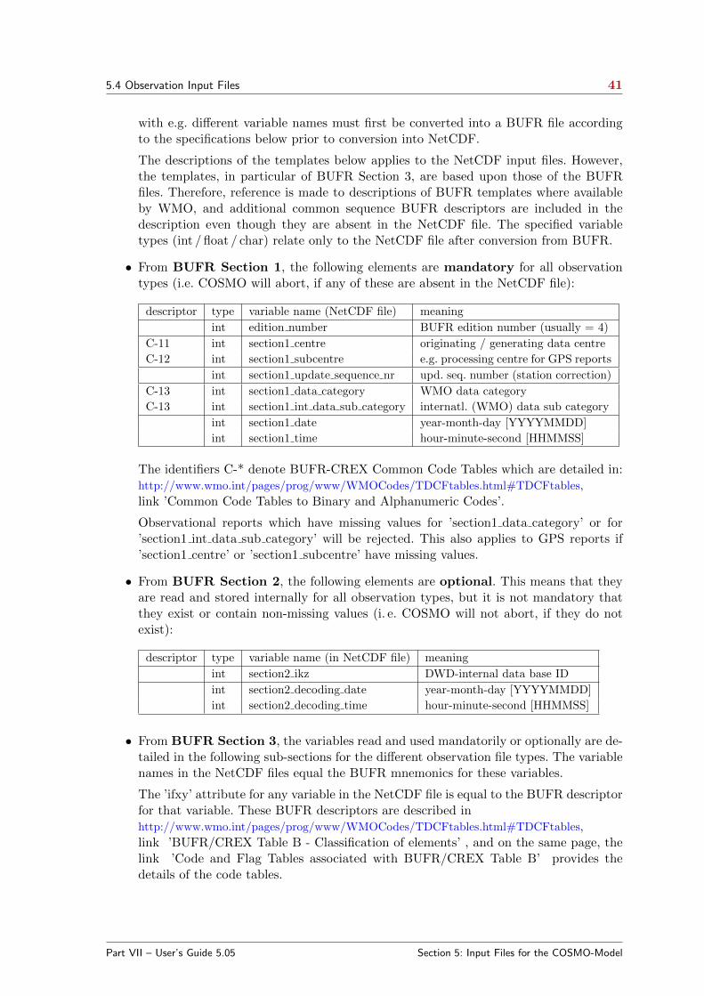
5.4 Observation Input Files 41
with e.g. different variable names must first be converted into a BUFR file accordingto the specifications below prior to conversion into NetCDF.
The descriptions of the templates below applies to the NetCDF input files. However,the templates, in particular of BUFR Section 3, are based upon those of the BUFRfiles. Therefore, reference is made to descriptions of BUFR templates where availableby WMO, and additional common sequence BUFR descriptors are included in thedescription even though they are absent in the NetCDF file. The specified variabletypes (int / float / char) relate only to the NetCDF file after conversion from BUFR.
• From BUFR Section 1, the following elements are mandatory for all observationtypes (i.e. COSMO will abort, if any of these are absent in the NetCDF file):
descriptor type variable name (NetCDF file) meaning
int edition number BUFR edition number (usually = 4)
C-11 int section1 centre originating / generating data centre
C-12 int section1 subcentre e.g. processing centre for GPS reports
int section1 update sequence nr upd. seq. number (station correction)
C-13 int section1 data category WMO data category
C-13 int section1 int data sub category internatl. (WMO) data sub category
int section1 date year-month-day [YYYYMMDD]
int section1 time hour-minute-second [HHMMSS]
The identifiers C-* denote BUFR-CREX Common Code Tables which are detailed in:http://www.wmo.int/pages/prog/www/WMOCodes/TDCFtables.html#TDCFtables,
link ’Common Code Tables to Binary and Alphanumeric Codes’.
Observational reports which have missing values for ’section1 data category’ or for’section1 int data sub category’ will be rejected. This also applies to GPS reports if’section1 centre’ or ’section1 subcentre’ have missing values.
• From BUFR Section 2, the following elements are optional. This means that theyare read and stored internally for all observation types, but it is not mandatory thatthey exist or contain non-missing values (i. e. COSMO will not abort, if they do notexist):
descriptor type variable name (in NetCDF file) meaning
int section2 ikz DWD-internal data base ID
int section2 decoding date year-month-day [YYYYMMDD]
int section2 decoding time hour-minute-second [HHMMSS]
• From BUFR Section 3, the variables read and used mandatorily or optionally are de-tailed in the following sub-sections for the different observation file types. The variablenames in the NetCDF files equal the BUFR mnemonics for these variables.
The ’ifxy’ attribute for any variable in the NetCDF file is equal to the BUFR descriptorfor that variable. These BUFR descriptors are described inhttp://www.wmo.int/pages/prog/www/WMOCodes/TDCFtables.html#TDCFtables,
link ’BUFR/CREX Table B - Classification of elements’ , and on the same page, thelink ’Code and Flag Tables associated with BUFR/CREX Table B’ provides thedetails of the code tables.
Part VII – User’s Guide 5.05 Section 5: Input Files for the COSMO-Model

5.4 Observation Input Files 42
Observational reports are rejected unless they contain appropriate non-missing valuesfor observation time (year, month, day, hour, minute), location (latitude, longitude),and for some observation types station altitude and some form of station identity.
Note that for some observation file types, the (BUFR and the) NetCDF files producedat DWD contain an additional variable for each (or most) of the existing variablesof section 3. This variable contains a quality flag related to the value of the originalvariable. The variable name of this quality flag variable is equal to the name of theoriginal variable plus a suffix ’Q’. However, all the quality flag variables of this typeare obsolete, i.e. they are never needed, never used or read by COSMO, they alwayscontain missing values only, and therefore they are never described hereafter.
In the following sub-sections of this section, the sequences of variables (templates) relatedto BUFR Section 3 are detailed for the different observation types. In the last sub-section,the blacklist file is described.
5.4.1 Templates for observation types for which Table-Driven Code Forms(TDCF) defined by WMO exist
The BUFR templates, which the NetCDF files described in this sub-section are based on,are described athttp://www.wmo.int/pages/prog/www/WMOCodes/TemplateExamples.html.
• SYNOP, SYNOP MOBIL, and SHIP
File names: for fixed land stations (SYNOP) : ’cdfin synop’
for mobile land stations (SYNOP MOBIL) : ’cdfin synop mob’
for sea stations (SHIP) : ’cdfin ship’.
The templates for observation type SYNOP and for SYNOP MOBIL follow the WMOcommon sequence descriptors ’TM 3 07 080’ resp. ’TM 3 07 090’. These sequences,and also the use of the variables in COSMO, are identical to each other except forthe report header (common sequences ’3 01 090’ esp. ’3 01 092’). The template for SHIPfollows the WMO common sequence descriptor ’TM 3 08 009’.
Caution: The use of observation file type ’SYNOP MOBIL’ in COSMO has not beentested yet due to a lack of testing opportunity because of a lack of data of this type. Itsuse is at the user’s own risk. However, as the template is almost the same as for fixedland SYNOP, errors are unlikely. If errors occur, they should be reported to the author.
For all the 3 observation (file) types, the table below lists all the variables which areused by COSMO, plus some of the other variables, but it does not detail the variablesfor those common sequences which contain only variables that are not used by COSMO.For convenience, the table is split into a report header and three report body parts.
The use of the variables (first column of table) is defined as follows:
Part VII – User’s Guide 5.05 Section 5: Input Files for the COSMO-Model

5.4 Observation Input Files 43
’need’: COSMO asks stringently for this variable and will abort if variable is absent(but will not abort if values are equal to ’missing value’)
’opt’: variable exists and is read/used (but COSMO will not abort if it does notexist); ’used’ means here that it is e. g. written to the feedobs file, but itdoes not imply active use in the data assimilation
’+’: variable exists but is not read by COSMO
’−’: descriptor (a BUFR common sequence, or a BUFR data description oper-ator) exists only in the BUFR file, not in the NetCDF file
’(−)’: descriptor itself exists only in the BUFR file, not in the NetCDF file; how-ever the descriptor indicates a common sequence of variables, which arepresent in the NetCDF file, but which are not used by COSMO and henceare not detailed here
The existence (2nd column ’L’ for land stations, 3rd column ’S’ for SHIP sea stations)of the variables or descriptors for the different observation (file) types according to theabove mentioned BUFR common sequence descriptors is defined as follows:
’+’ : exists (for both types of land stations resp. for sea stations)
’f’ : exists for fixed land stations, but not for mobile land stations
’m’ : exists for mobile land stations, but not for fixed land stations
’ ’ : does not exist
use L S WMO type mnemonics meaning
descriptor
− f 3 01 090 Fixed surface station ID, time,horiz. + vertical coordinates
− m 3 01 092 Mobile surface station ID, time,horiz. + vertical coordinates
− + 3 01 093 Ship ID, movement, date / time,horiz. + vertical coordinates
− + 3 01 036 Ship ID, movement, time, lat/lon
need m + 0 01 011 char*9 YDDDD Ship or mobile land sta. identifier
+ + 0 01 012 int MDS Platform motion direction
+ + 0 01 013 int NVS Platform motion speed
+ m 0 01 003 int MA WMO region number
− f 3 01 004 Surface station identification
need f 0 01 001 int MII WMO block number
need f 0 01 002 int NIII WMO station number
opt f 0 01 015 char*20 YSOSN Station or site name
need + + 0 02 001 int NIX Type of station
− + 3 01 011 Year, month and day
need + + 0 04 001 int MJJJ Year
need + + 0 04 002 int MMM Month
need + + 0 04 003 int MYY Day
− + 3 01 012 Hour, minute
need + + 0 04 004 int MGG Hour
need + + 0 04 005 int NGG Minute
− + 3 01 021 Latitude and Longitude
need + 0 05 001 float MLAH Latitude (high accuracy) [degree]
need + 0 06 001 float MLOH Longitude (high accuracy) [deg.]
need + 0 05 002 float MLALA Latitude (coarse accuracy) [deg.]
Part VII – User’s Guide 5.05 Section 5: Input Files for the COSMO-Model

5.4 Observation Input Files 44
use L S WMO type mnemonics meaning
descriptor
need + 0 06 002 float MLOLO Longitude (coarse accur.) [deg.]
need + + 0 07 030 float MHOSNN Height of station above MSL (1)
need + + 0 07 031 float MHOBNN Height of barometer a. MSL (1)
opt m 0 33 024 int MSEQM Station elevation quality mark
− + 3 02 031 Pressure data
− + + 3 02 001 Pressure group
need + + 0 10 004 float MPPP Pressure
opt + + 0 10 051 float MPPPP Pressure reduced to MSL
opt + + 0 10 061 float NPPP 3-hour pressure change
+ + + 0 10 063 int NA Characteristic of press. tendency
+ + 0 10 062 float NP24 24-hour pressure change
opt + 0 07 004 float MPN Pressure (standard level)
opt + 0 10 009 int NHHHN Geopotential height [gpm] ofthe standard level
− + 3 02 035 Basic synoptic ’instanteous’ data− + 3 02 054 SHIP ’instanteous’ data
− + 3 02 032Temperature + humidity data− + 3 02 052
opt + + 0 07 032 float MHOSEN Height of sensor above localground / marine deck platform(for temp. + humidity meas.)
opt + 0 07 033 float MHAWAS Height of sensor above watersurface (temp. + hum. meas.)
need + + 0 12 101 float MTDBT Temperature / dry-bulb temperat.
+ + 0 02 039 int MMOWTM Method of wet-bulb temp. meas.
+ + 0 12 102 float MTFNH Wet-bulb temperature
need + + 0 12 103 float MTDNH Dew-point temperature
opt + + 0 13 003 int MUUU Relative humidity [%]
− + 3 02 033Visibility data− + 3 02 053
+ + + 0 07 032 float MHOSEN0 Height of sensor a. ground (vis.)
opt + 0 07 033 float MHAWAS0 Height of sensor above watersurface (for visibility)
opt + + 0 20 001 float MVV Horizontal visibility
− + + 3 02 034 Precipitation past 24 hours
+ + + 0 07 032 float MHOSEN1 Height of sensor a. gr. (precip.)
opt + + 0 13 023 float MRR24 Total precipitation past 24 hours
− + + 3 02 004 Cloud data
opt + + 0 20 010 int MN Cloud cover (total) [%]
opt + + 0 08 002 int MVTSU Vertical significance
opt + + 0 20 011 int MNH Cloud amount(of low or middle clouds)
opt + + 0 20 013 float NH Cloud base height above surface
opt + + 0 20 012 int MCC Cloud type (low clouds CL)
opt + + 0 20 012 int MCC0 Cloud type (middle clouds CM )
opt + + 0 20 012 int MCC1 Cloud type (high clouds CH)
opt + + 0 31 001 int MDREP Delayed descriptor replication
− + + 3 02 005 Individual cloud layers of masses
opt + + 0 08 002 int *n MVTSU0 Vertical significance (2)
Part VII – User’s Guide 5.05 Section 5: Input Files for the COSMO-Model
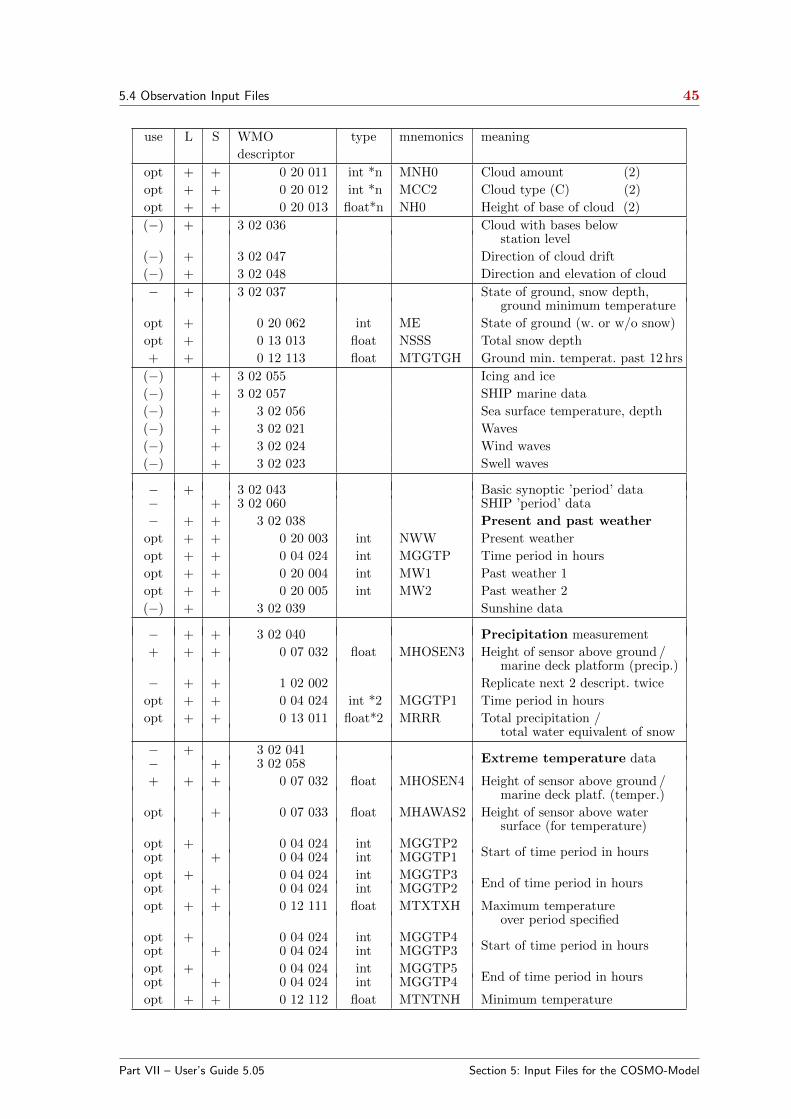
5.4 Observation Input Files 45
use L S WMO type mnemonics meaning
descriptor
opt + + 0 20 011 int *n MNH0 Cloud amount (2)
opt + + 0 20 012 int *n MCC2 Cloud type (C) (2)
opt + + 0 20 013 float*n NH0 Height of base of cloud (2)
(−) + 3 02 036 Cloud with bases belowstation level
(−) + 3 02 047 Direction of cloud drift
(−) + 3 02 048 Direction and elevation of cloud
− + 3 02 037 State of ground, snow depth,ground minimum temperature
opt + 0 20 062 int ME State of ground (w. or w/o snow)
opt + 0 13 013 float NSSS Total snow depth
+ + 0 12 113 float MTGTGH Ground min. temperat. past 12 hrs
(−) + 3 02 055 Icing and ice
(−) + 3 02 057 SHIP marine data
(−) + 3 02 056 Sea surface temperature, depth
(−) + 3 02 021 Waves
(−) + 3 02 024 Wind waves
(−) + 3 02 023 Swell waves
− + 3 02 043 Basic synoptic ’period’ data− + 3 02 060 SHIP ’period’ data
− + + 3 02 038 Present and past weather
opt + + 0 20 003 int NWW Present weather
opt + + 0 04 024 int MGGTP Time period in hours
opt + + 0 20 004 int MW1 Past weather 1
opt + + 0 20 005 int MW2 Past weather 2
(−) + 3 02 039 Sunshine data
− + + 3 02 040 Precipitation measurement
+ + + 0 07 032 float MHOSEN3 Height of sensor above ground /marine deck platform (precip.)
− + + 1 02 002 Replicate next 2 descript. twice
opt + + 0 04 024 int *2 MGGTP1 Time period in hours
opt + + 0 13 011 float*2 MRRR Total precipitation /total water equivalent of snow
− + 3 02 041Extreme temperature data− + 3 02 058
+ + + 0 07 032 float MHOSEN4 Height of sensor above ground /marine deck platf. (temper.)
opt + 0 07 033 float MHAWAS2 Height of sensor above watersurface (for temperature)
opt + 0 04 024 int MGGTP2Start of time period in hoursopt + 0 04 024 int MGGTP1
opt + 0 04 024 int MGGTP3End of time period in hoursopt + 0 04 024 int MGGTP2
opt + + 0 12 111 float MTXTXH Maximum temperatureover period specified
opt + 0 04 024 int MGGTP4Start of time period in hoursopt + 0 04 024 int MGGTP3
opt + 0 04 024 int MGGTP5End of time period in hoursopt + 0 04 024 int MGGTP4
opt + + 0 12 112 float MTNTNH Minimum temperature
Part VII – User’s Guide 5.05 Section 5: Input Files for the COSMO-Model
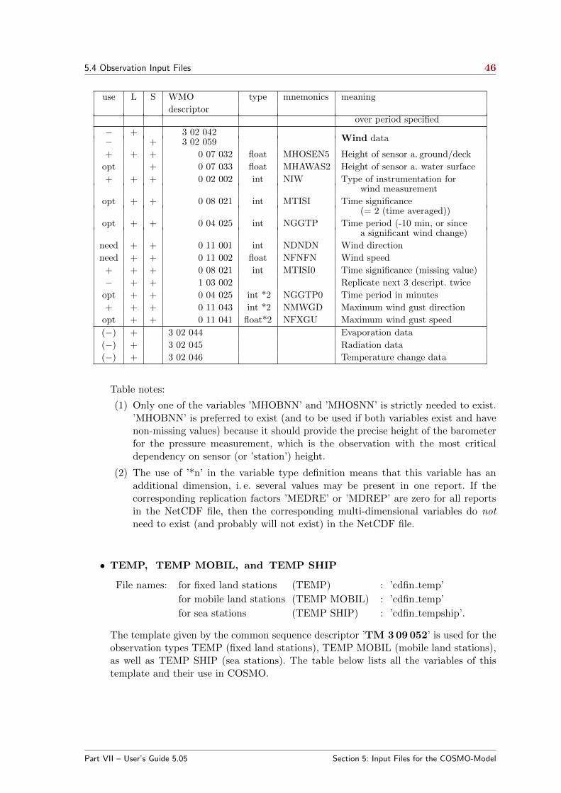
5.4 Observation Input Files 46
use L S WMO type mnemonics meaning
descriptorover period specified
− + 3 02 042Wind data− + 3 02 059
+ + + 0 07 032 float MHOSEN5 Height of sensor a. ground/deck
opt + 0 07 033 float MHAWAS2 Height of sensor a. water surface
+ + + 0 02 002 int NIW Type of instrumentation forwind measurement
opt + + 0 08 021 int MTISI Time significance(= 2 (time averaged))
opt + + 0 04 025 int NGGTP Time period (-10 min, or sincea significant wind change)
need + + 0 11 001 int NDNDN Wind direction
need + + 0 11 002 float NFNFN Wind speed
+ + + 0 08 021 int MTISI0 Time significance (missing value)
− + + 1 03 002 Replicate next 3 descript. twice
opt + + 0 04 025 int *2 NGGTP0 Time period in minutes
+ + + 0 11 043 int *2 NMWGD Maximum wind gust direction
opt + + 0 11 041 float*2 NFXGU Maximum wind gust speed
(−) + 3 02 044 Evaporation data
(−) + 3 02 045 Radiation data
(−) + 3 02 046 Temperature change data
Table notes:
(1) Only one of the variables ’MHOBNN’ and ’MHOSNN’ is strictly needed to exist.’MHOBNN’ is preferred to exist (and to be used if both variables exist and havenon-missing values) because it should provide the precise height of the barometerfor the pressure measurement, which is the observation with the most criticaldependency on sensor (or ’station’) height.
(2) The use of ’*n’ in the variable type definition means that this variable has anadditional dimension, i. e. several values may be present in one report. If thecorresponding replication factors ’MEDRE’ or ’MDREP’ are zero for all reportsin the NetCDF file, then the corresponding multi-dimensional variables do notneed to exist (and probably will not exist) in the NetCDF file.
• TEMP, TEMP MOBIL, and TEMP SHIP
File names: for fixed land stations (TEMP) : ’cdfin temp’
for mobile land stations (TEMP MOBIL) : ’cdfin temp’
for sea stations (TEMP SHIP) : ’cdfin tempship’.
The template given by the common sequence descriptor ’TM 3 09 052’ is used for theobservation types TEMP (fixed land stations), TEMP MOBIL (mobile land stations),as well as TEMP SHIP (sea stations). The table below lists all the variables of thistemplate and their use in COSMO.
Part VII – User’s Guide 5.05 Section 5: Input Files for the COSMO-Model

5.4 Observation Input Files 47
The use of the variables (first column of table) is defined as follows:
’need’: COSMO asks stringently for this variable and will abort if variable is absent(but will not abort if values are equal to ’missing value’)
’opt’: variable exists and is read/used (but COSMO will not abort if it does notexist); ’used’ means here that it is e. g. written to the feedobs file, but itdoes not imply active use in the data assimilation
’+’: variable exists but is not read by COSMO
’−’: descriptor (a BUFR common sequence, or a BUFR data description oper-ator) exists only in the BUFR file, not in the NetCDF file
use WMO type mnemonics meaning
descriptor
− 3 01 111 Identific. of launch site + instumentation
− 3 01 001 Station identification
need 0 01 001 int MII WMO block number (1)
need 0 01 002 int NIII WMO station number (1)
need 0 01 011 char*9 YDDDD Ship or mobile land station identifier (1)
need 0 02 011 int NRARA Radiosonde type
opt 0 02 013 int NSR Solar and infrared radiation correction
opt 0 02 014 int NSASA Tracking technique / status of system
opt 0 02 003 int NA4 Type of measuring equipment
− 3 01 113 Date / time of launch
opt 0 08 021 int MTISI Time significance (= 18 (launch time))
− 3 01 011 Year, month and day
need 0 04 001 int MJJJ Year
need 0 04 002 int MMM Month
need 0 04 003 int MYY Day
− 3 01 013 Hour, minute, second
need 0 04 004 int MGG Hour
need 0 04 005 int NGG Minute
+ 0 04 006 int MSEC Second
− 3 01 114 Horiz. + vert. coord. of launch site
− 3 01 021 Latitude and Longitude
need 0 05 001 float MLAH Latitude (high accuracy) [degree]
need 0 06 001 float MLOH Longitude (high accuracy) [degree]
need 0 07 030 float MHOSNN Height of station above MSL (2)
need 0 07 031 float MHOBNN Height of barometer above MSL (2)
opt 0 07 007 int MH Height of release of sonde above MSL
opt 0 33 024 int MSEQM Station elevation quality mark
− 3 02 049 Cloud info reported with vert. soundings
opt 0 08 002 int MVTSU Vertical significance
opt 0 20 011 int MNH Cloud amount (of low or middle clouds)
opt 0 20 013 float NH Cloud base height above surface
opt 0 20 012 int MCC Cloud type (low clouds CL)
opt 0 20 012 int MCC0 Cloud type (middle clouds CM )
opt 0 20 012 int MCC1 Cloud type (high clouds CH)
+ 0 22 043 float MTN00 Sea / water temperature
need 0 31 002 int MEDRE Extended delayed descriptor replicat. fac.
− 3 03 054 Temperature, dewpoint + wind data
Part VII – User’s Guide 5.05 Section 5: Input Files for the COSMO-Model
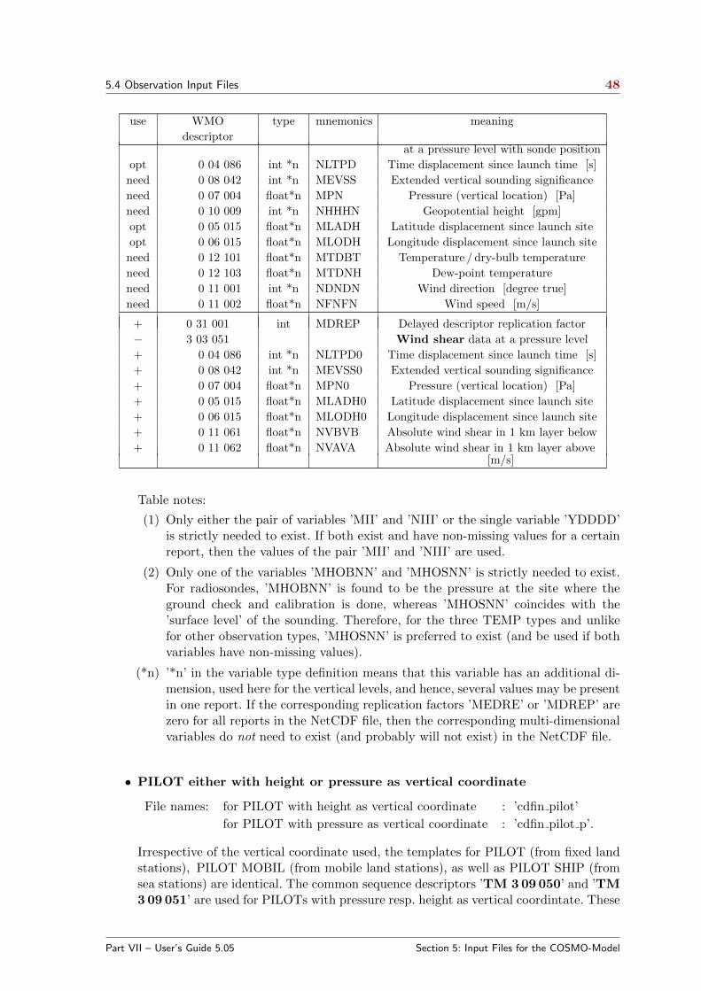
5.4 Observation Input Files 48
use WMO type mnemonics meaning
descriptorat a pressure level with sonde position
opt 0 04 086 int *n NLTPD Time displacement since launch time [s]
need 0 08 042 int *n MEVSS Extended vertical sounding significance
need 0 07 004 float*n MPN Pressure (vertical location) [Pa]
need 0 10 009 int *n NHHHN Geopotential height [gpm]
opt 0 05 015 float*n MLADH Latitude displacement since launch site
opt 0 06 015 float*n MLODH Longitude displacement since launch site
need 0 12 101 float*n MTDBT Temperature / dry-bulb temperature
need 0 12 103 float*n MTDNH Dew-point temperature
need 0 11 001 int *n NDNDN Wind direction [degree true]
need 0 11 002 float*n NFNFN Wind speed [m/s]
+ 0 31 001 int MDREP Delayed descriptor replication factor
− 3 03 051 Wind shear data at a pressure level
+ 0 04 086 int *n NLTPD0 Time displacement since launch time [s]
+ 0 08 042 int *n MEVSS0 Extended vertical sounding significance
+ 0 07 004 float*n MPN0 Pressure (vertical location) [Pa]
+ 0 05 015 float*n MLADH0 Latitude displacement since launch site
+ 0 06 015 float*n MLODH0 Longitude displacement since launch site
+ 0 11 061 float*n NVBVB Absolute wind shear in 1 km layer below
+ 0 11 062 float*n NVAVA Absolute wind shear in 1 km layer above[m/s]
Table notes:
(1) Only either the pair of variables ’MII’ and ’NIII’ or the single variable ’YDDDD’is strictly needed to exist. If both exist and have non-missing values for a certainreport, then the values of the pair ’MII’ and ’NIII’ are used.
(2) Only one of the variables ’MHOBNN’ and ’MHOSNN’ is strictly needed to exist.For radiosondes, ’MHOBNN’ is found to be the pressure at the site where theground check and calibration is done, whereas ’MHOSNN’ coincides with the’surface level’ of the sounding. Therefore, for the three TEMP types and unlikefor other observation types, ’MHOSNN’ is preferred to exist (and be used if bothvariables have non-missing values).
(*n) ’*n’ in the variable type definition means that this variable has an additional di-mension, used here for the vertical levels, and hence, several values may be presentin one report. If the corresponding replication factors ’MEDRE’ or ’MDREP’ arezero for all reports in the NetCDF file, then the corresponding multi-dimensionalvariables do not need to exist (and probably will not exist) in the NetCDF file.
• PILOT either with height or pressure as vertical coordinate
File names: for PILOT with height as vertical coordinate : ’cdfin pilot’
for PILOT with pressure as vertical coordinate : ’cdfin pilot p’.
Irrespective of the vertical coordinate used, the templates for PILOT (from fixed landstations), PILOT MOBIL (from mobile land stations), as well as PILOT SHIP (fromsea stations) are identical. The common sequence descriptors ’TM 3 09 050’ and ’TM3 09 051’ are used for PILOTs with pressure resp. height as vertical coordintate. These
Part VII – User’s Guide 5.05 Section 5: Input Files for the COSMO-Model
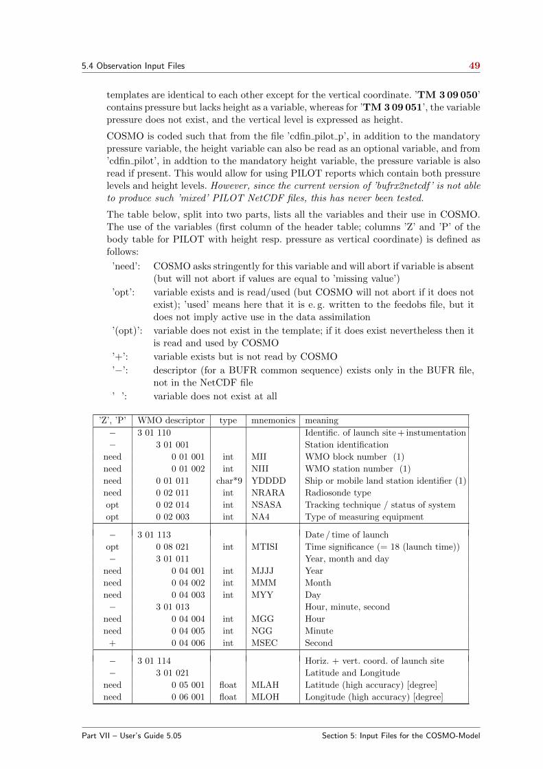
5.4 Observation Input Files 49
templates are identical to each other except for the vertical coordinate. ’TM 3 09 050’contains pressure but lacks height as a variable, whereas for ’TM 3 09 051’, the variablepressure does not exist, and the vertical level is expressed as height.
COSMO is coded such that from the file ’cdfin pilot p’, in addition to the mandatorypressure variable, the height variable can also be read as an optional variable, and from’cdfin pilot’, in addtion to the mandatory height variable, the pressure variable is alsoread if present. This would allow for using PILOT reports which contain both pressurelevels and height levels. However, since the current version of ’bufrx2netcdf’ is not ableto produce such ’mixed’ PILOT NetCDF files, this has never been tested.
The table below, split into two parts, lists all the variables and their use in COSMO.The use of the variables (first column of the header table; columns ’Z’ and ’P’ of thebody table for PILOT with height resp. pressure as vertical coordinate) is defined asfollows:
’need’: COSMO asks stringently for this variable and will abort if variable is absent(but will not abort if values are equal to ’missing value’)
’opt’: variable exists and is read/used (but COSMO will not abort if it does notexist); ’used’ means here that it is e. g. written to the feedobs file, but itdoes not imply active use in the data assimilation
’(opt)’: variable does not exist in the template; if it does exist nevertheless then itis read and used by COSMO
’+’: variable exists but is not read by COSMO
’−’: descriptor (for a BUFR common sequence) exists only in the BUFR file,not in the NetCDF file
’ ’: variable does not exist at all
’Z’, ’P’ WMO descriptor type mnemonics meaning
− 3 01 110 Identific. of launch site + instumentation
− 3 01 001 Station identification
need 0 01 001 int MII WMO block number (1)
need 0 01 002 int NIII WMO station number (1)
need 0 01 011 char*9 YDDDD Ship or mobile land station identifier (1)
need 0 02 011 int NRARA Radiosonde type
opt 0 02 014 int NSASA Tracking technique / status of system
opt 0 02 003 int NA4 Type of measuring equipment
− 3 01 113 Date / time of launch
opt 0 08 021 int MTISI Time significance (= 18 (launch time))
− 3 01 011 Year, month and day
need 0 04 001 int MJJJ Year
need 0 04 002 int MMM Month
need 0 04 003 int MYY Day
− 3 01 013 Hour, minute, second
need 0 04 004 int MGG Hour
need 0 04 005 int NGG Minute
+ 0 04 006 int MSEC Second
− 3 01 114 Horiz. + vert. coord. of launch site
− 3 01 021 Latitude and Longitude
need 0 05 001 float MLAH Latitude (high accuracy) [degree]
need 0 06 001 float MLOH Longitude (high accuracy) [degree]
Part VII – User’s Guide 5.05 Section 5: Input Files for the COSMO-Model
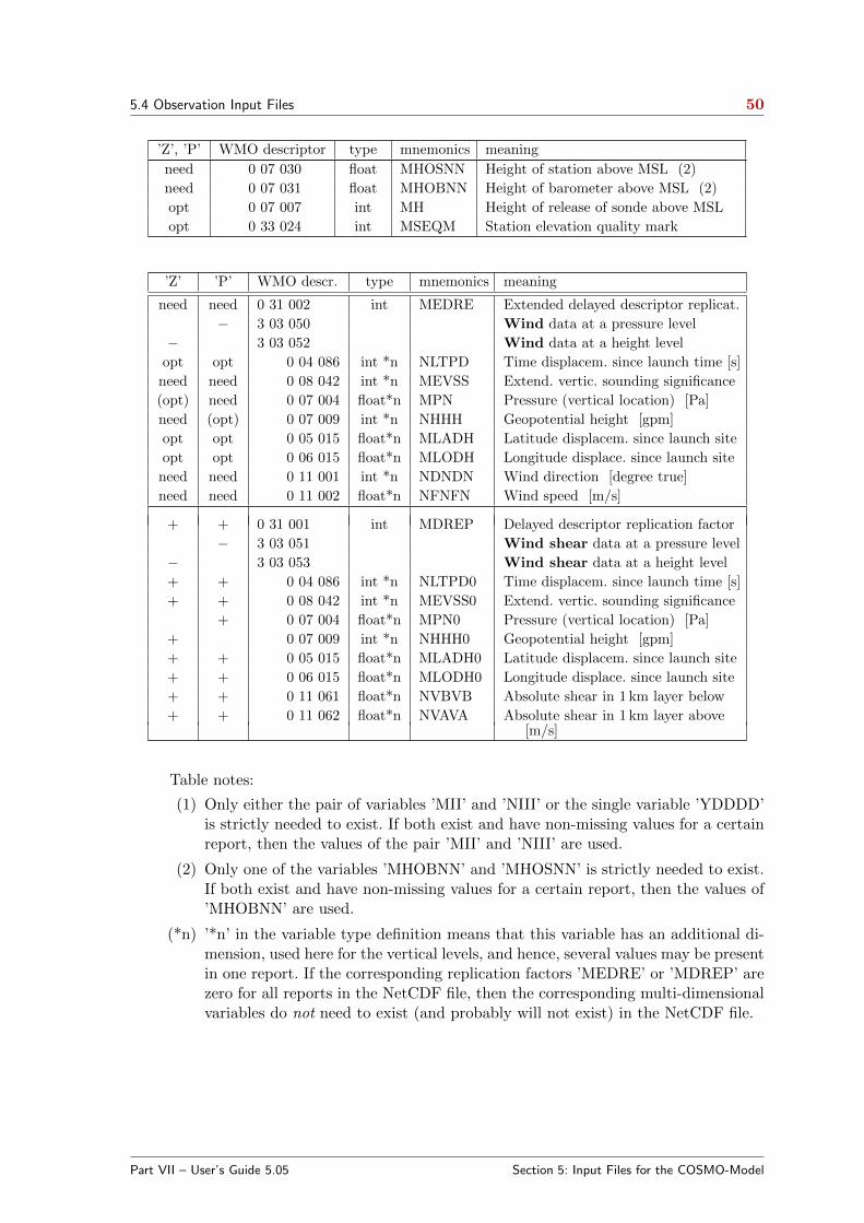
5.4 Observation Input Files 50
’Z’, ’P’ WMO descriptor type mnemonics meaning
need 0 07 030 float MHOSNN Height of station above MSL (2)
need 0 07 031 float MHOBNN Height of barometer above MSL (2)
opt 0 07 007 int MH Height of release of sonde above MSL
opt 0 33 024 int MSEQM Station elevation quality mark
’Z’ ’P’ WMO descr. type mnemonics meaning
need need 0 31 002 int MEDRE Extended delayed descriptor replicat.
− 3 03 050 Wind data at a pressure level
− 3 03 052 Wind data at a height level
opt opt 0 04 086 int *n NLTPD Time displacem. since launch time [s]
need need 0 08 042 int *n MEVSS Extend. vertic. sounding significance
(opt) need 0 07 004 float*n MPN Pressure (vertical location) [Pa]
need (opt) 0 07 009 int *n NHHH Geopotential height [gpm]
opt opt 0 05 015 float*n MLADH Latitude displacem. since launch site
opt opt 0 06 015 float*n MLODH Longitude displace. since launch site
need need 0 11 001 int *n NDNDN Wind direction [degree true]
need need 0 11 002 float*n NFNFN Wind speed [m/s]
+ + 0 31 001 int MDREP Delayed descriptor replication factor
− 3 03 051 Wind shear data at a pressure level
− 3 03 053 Wind shear data at a height level
+ + 0 04 086 int *n NLTPD0 Time displacem. since launch time [s]
+ + 0 08 042 int *n MEVSS0 Extend. vertic. sounding significance
+ 0 07 004 float*n MPN0 Pressure (vertical location) [Pa]
+ 0 07 009 int *n NHHH0 Geopotential height [gpm]
+ + 0 05 015 float*n MLADH0 Latitude displacem. since launch site
+ + 0 06 015 float*n MLODH0 Longitude displace. since launch site
+ + 0 11 061 float*n NVBVB Absolute shear in 1 km layer below
+ + 0 11 062 float*n NVAVA Absolute shear in 1 km layer above[m/s]
Table notes:
(1) Only either the pair of variables ’MII’ and ’NIII’ or the single variable ’YDDDD’is strictly needed to exist. If both exist and have non-missing values for a certainreport, then the values of the pair ’MII’ and ’NIII’ are used.
(2) Only one of the variables ’MHOBNN’ and ’MHOSNN’ is strictly needed to exist.If both exist and have non-missing values for a certain report, then the values of’MHOBNN’ are used.
(*n) ’*n’ in the variable type definition means that this variable has an additional di-mension, used here for the vertical levels, and hence, several values may be presentin one report. If the corresponding replication factors ’MEDRE’ or ’MDREP’ arezero for all reports in the NetCDF file, then the corresponding multi-dimensionalvariables do not need to exist (and probably will not exist) in the NetCDF file.
Part VII – User’s Guide 5.05 Section 5: Input Files for the COSMO-Model
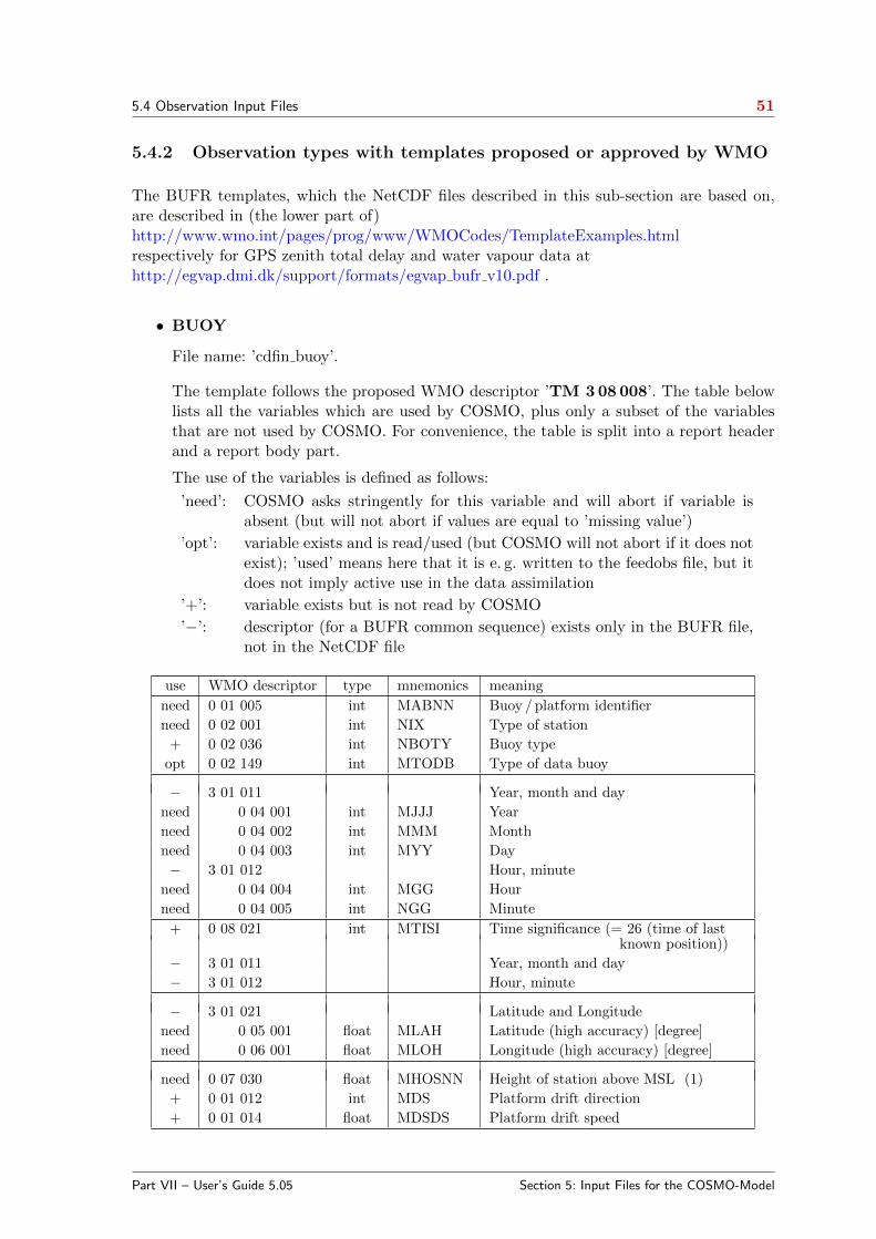
5.4 Observation Input Files 51
5.4.2 Observation types with templates proposed or approved by WMO
The BUFR templates, which the NetCDF files described in this sub-section are based on,are described in (the lower part of)http://www.wmo.int/pages/prog/www/WMOCodes/TemplateExamples.htmlrespectively for GPS zenith total delay and water vapour data athttp://egvap.dmi.dk/support/formats/egvap bufr v10.pdf .
• BUOY
File name: ’cdfin buoy’.
The template follows the proposed WMO descriptor ’TM 3 08 008’. The table belowlists all the variables which are used by COSMO, plus only a subset of the variablesthat are not used by COSMO. For convenience, the table is split into a report headerand a report body part.
The use of the variables is defined as follows:
’need’: COSMO asks stringently for this variable and will abort if variable isabsent (but will not abort if values are equal to ’missing value’)
’opt’: variable exists and is read/used (but COSMO will not abort if it does notexist); ’used’ means here that it is e. g. written to the feedobs file, but itdoes not imply active use in the data assimilation
’+’: variable exists but is not read by COSMO
’−’: descriptor (for a BUFR common sequence) exists only in the BUFR file,not in the NetCDF file
use WMO descriptor type mnemonics meaning
need 0 01 005 int MABNN Buoy / platform identifier
need 0 02 001 int NIX Type of station
+ 0 02 036 int NBOTY Buoy type
opt 0 02 149 int MTODB Type of data buoy
− 3 01 011 Year, month and day
need 0 04 001 int MJJJ Year
need 0 04 002 int MMM Month
need 0 04 003 int MYY Day
− 3 01 012 Hour, minute
need 0 04 004 int MGG Hour
need 0 04 005 int NGG Minute
+ 0 08 021 int MTISI Time significance (= 26 (time of lastknown position))
− 3 01 011 Year, month and day
− 3 01 012 Hour, minute
− 3 01 021 Latitude and Longitude
need 0 05 001 float MLAH Latitude (high accuracy) [degree]
need 0 06 001 float MLOH Longitude (high accuracy) [degree]
need 0 07 030 float MHOSNN Height of station above MSL (1)
+ 0 01 012 int MDS Platform drift direction
+ 0 01 014 float MDSDS Platform drift speed
Part VII – User’s Guide 5.05 Section 5: Input Files for the COSMO-Model
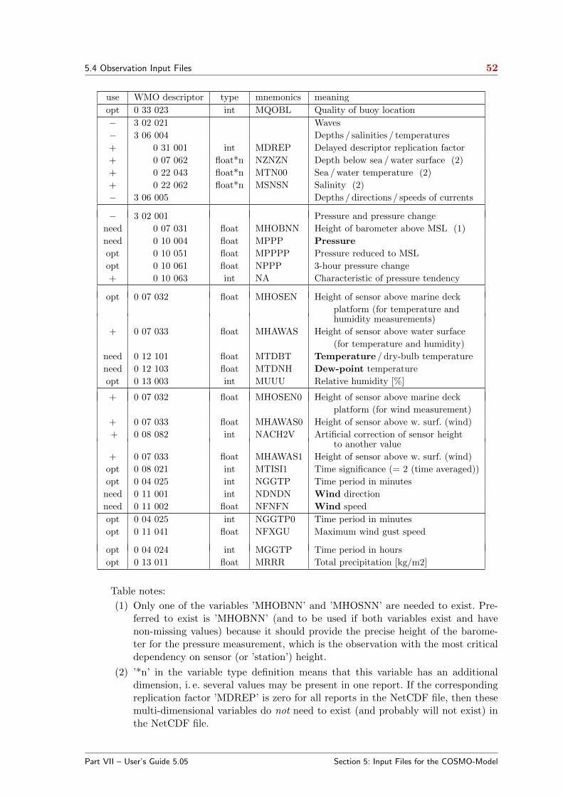
5.4 Observation Input Files 52
use WMO descriptor type mnemonics meaning
opt 0 33 023 int MQOBL Quality of buoy location
− 3 02 021 Waves
− 3 06 004 Depths / salinities / temperatures
+ 0 31 001 int MDREP Delayed descriptor replication factor
+ 0 07 062 float*n NZNZN Depth below sea / water surface (2)
+ 0 22 043 float*n MTN00 Sea / water temperature (2)
+ 0 22 062 float*n MSNSN Salinity (2)
− 3 06 005 Depths / directions / speeds of currents
− 3 02 001 Pressure and pressure change
need 0 07 031 float MHOBNN Height of barometer above MSL (1)
need 0 10 004 float MPPP Pressure
opt 0 10 051 float MPPPP Pressure reduced to MSL
opt 0 10 061 float NPPP 3-hour pressure change
+ 0 10 063 int NA Characteristic of pressure tendency
opt 0 07 032 float MHOSEN Height of sensor above marine deck
platform (for temperature andhumidity measurements)
+ 0 07 033 float MHAWAS Height of sensor above water surface
(for temperature and humidity)
need 0 12 101 float MTDBT Temperature / dry-bulb temperature
need 0 12 103 float MTDNH Dew-point temperature
opt 0 13 003 int MUUU Relative humidity [%]
+ 0 07 032 float MHOSEN0 Height of sensor above marine deck
platform (for wind measurement)
+ 0 07 033 float MHAWAS0 Height of sensor above w. surf. (wind)
+ 0 08 082 int NACH2V Artificial correction of sensor heightto another value
+ 0 07 033 float MHAWAS1 Height of sensor above w. surf. (wind)
opt 0 08 021 int MTISI1 Time significance (= 2 (time averaged))
opt 0 04 025 int NGGTP Time period in minutes
need 0 11 001 int NDNDN Wind direction
need 0 11 002 float NFNFN Wind speed
opt 0 04 025 int NGGTP0 Time period in minutes
opt 0 11 041 float NFXGU Maximum wind gust speed
opt 0 04 024 int MGGTP Time period in hours
opt 0 13 011 float MRRR Total precipitation [kg/m2]
Table notes:
(1) Only one of the variables ’MHOBNN’ and ’MHOSNN’ are needed to exist. Pre-ferred to exist is ’MHOBNN’ (and to be used if both variables exist and havenon-missing values) because it should provide the precise height of the barome-ter for the pressure measurement, which is the observation with the most criticaldependency on sensor (or ’station’) height.
(2) ’*n’ in the variable type definition means that this variable has an additionaldimension, i. e. several values may be present in one report. If the correspondingreplication factor ’MDREP’ is zero for all reports in the NetCDF file, then thesemulti-dimensional variables do not need to exist (and probably will not exist) inthe NetCDF file.
Part VII – User’s Guide 5.05 Section 5: Input Files for the COSMO-Model
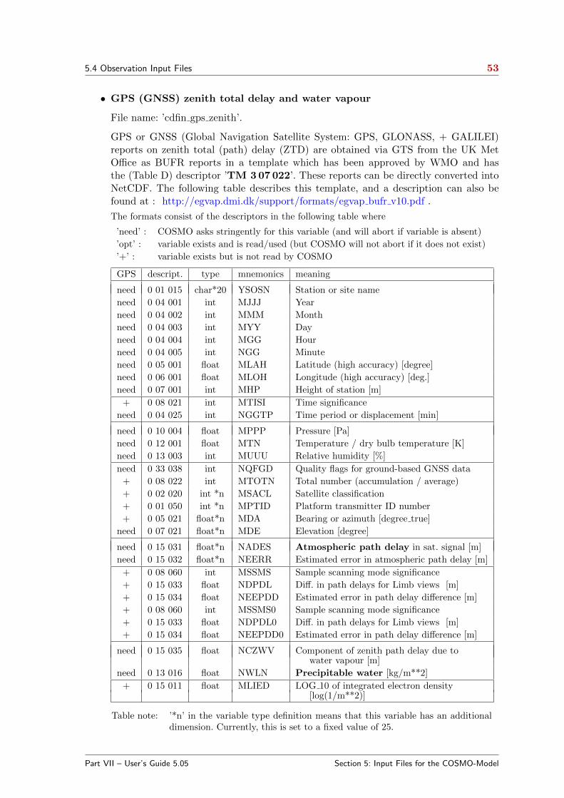
5.4 Observation Input Files 53
• GPS (GNSS) zenith total delay and water vapour
File name: ’cdfin gps zenith’.
GPS or GNSS (Global Navigation Satellite System: GPS, GLONASS, + GALILEI)reports on zenith total (path) delay (ZTD) are obtained via GTS from the UK MetOffice as BUFR reports in a template which has been approved by WMO and hasthe (Table D) descriptor ’TM 3 07 022’. These reports can be directly converted intoNetCDF. The following table describes this template, and a description can also befound at : http://egvap.dmi.dk/support/formats/egvap bufr v10.pdf .
The formats consist of the descriptors in the following table where
’need’ : COSMO asks stringently for this variable (and will abort if variable is absent)
’opt’ : variable exists and is read/used (but COSMO will not abort if it does not exist)
’+’ : variable exists but is not read by COSMO
GPS descript. type mnemonics meaning
need 0 01 015 char*20 YSOSN Station or site name
need 0 04 001 int MJJJ Year
need 0 04 002 int MMM Month
need 0 04 003 int MYY Day
need 0 04 004 int MGG Hour
need 0 04 005 int NGG Minute
need 0 05 001 float MLAH Latitude (high accuracy) [degree]
need 0 06 001 float MLOH Longitude (high accuracy) [deg.]
need 0 07 001 int MHP Height of station [m]
+ 0 08 021 int MTISI Time significance
need 0 04 025 int NGGTP Time period or displacement [min]
need 0 10 004 float MPPP Pressure [Pa]
need 0 12 001 float MTN Temperature / dry bulb temperature [K]
need 0 13 003 int MUUU Relative humidity [%]
need 0 33 038 int NQFGD Quality flags for ground-based GNSS data
+ 0 08 022 int MTOTN Total number (accumulation / average)
+ 0 02 020 int *n MSACL Satellite classification
+ 0 01 050 int *n MPTID Platform transmitter ID number
+ 0 05 021 float*n MDA Bearing or azimuth [degree true]
need 0 07 021 float*n MDE Elevation [degree]
need 0 15 031 float*n NADES Atmospheric path delay in sat. signal [m]
need 0 15 032 float*n NEERR Estimated error in atmospheric path delay [m]
+ 0 08 060 int MSSMS Sample scanning mode significance
+ 0 15 033 float NDPDL Diff. in path delays for Limb views [m]
+ 0 15 034 float NEEPDD Estimated error in path delay difference [m]
+ 0 08 060 int MSSMS0 Sample scanning mode significance
+ 0 15 033 float NDPDL0 Diff. in path delays for Limb views [m]
+ 0 15 034 float NEEPDD0 Estimated error in path delay difference [m]
need 0 15 035 float NCZWV Component of zenith path delay due towater vapour [m]
need 0 13 016 float NWLN Precipitable water [kg/m**2]
+ 0 15 011 float MLIED LOG 10 of integrated electron density[log(1/m**2)]
Table note: ’*n’ in the variable type definition means that this variable has an additionaldimension. Currently, this is set to a fixed value of 25.
Part VII – User’s Guide 5.05 Section 5: Input Files for the COSMO-Model

5.4 Observation Input Files 54
• GNSS zenith total delay
File name: ’cdfin gnss ztd’.
The GPS data described in the previous section can also be processed by the GNSSSTD operator. In contrast to the GPS IWV operator the STD operator is not partof the nudging assimilation system. The output of the STD operator is written to aspecific feedobs file fof gnssgb * but the model state is not modified.
In order to distinguish between both operators unique input file names are requiredeven if the contents of the files is identical.
• single-level AMDAR
File name: ’cdfin amdar’.
The template follows the proposed WMO descriptor ’TM 3 11 010’ and is describedin the table below. The use of the variables is defined as follows:
’need’ : COSMO asks stringently for this variable (and will abort if variable is absent)
’opt’ : variable exists and is read/used (but COSMO will not abort if it does not exist)
’+’ : variable exists but is not read by COSMO
’(+)’ : descriptor exists only in the BUFR file, not in the NetCDF file
use WMO descriptor type mnemonics meaning
use WMO descriptor type mnemonics meaning
+ 0 31 021 MADDF Associated field significance (1)
− 3 11 005 Standard AMDAR report
need 0 01 008 char*8 YAIRN Aircraft identification
+ 0 01 023 int NOSNO Observation sequence number
− 3 01 021 Latitude and Longitude
need 0 05 001 float MLAH Latitude (high accuracy) [degree]
need 0 06 001 float MLOH Longitude (high accuracy) [degree]
− 3 01 011 Year, month and day
need 0 04 001 int MJJJ Year
need 0 04 002 int MMM Month
need 0 04 003 int MYY Day
− 3 01 013 Hour, minute and second
need 0 04 004 int MGG Hour
need 0 04 005 int NGG Minute
+ 0 04 006 int MSEC Second
need 0 07 010 int NFLEV Flight level (2)
opt 0 08 009 int NDEPF Detailed phase of flight (3)
need 0 11 001 int NDNDN Wind direction
need 0 11 002 float NFNFN Wind speed
opt 0 11 031 int MB Degree of turbulence
opt 0 11 036 float NMDEWX Derived equivalent vertical gust speed
need 0 12 101 float MTDBT Temperature / dry-bulb T
+ 0 33 025 int MAIV ACARS interpolated values
need 0 08 004 int MPHAI Phase of flight
need 0 02 064 int MQARA Wind quality/roll angle
opt 0 13 003 int MUUU Relative humidity
need 0 12 103 float MTDNH Dew-point temperature
Part VII – User’s Guide 5.05 Section 5: Input Files for the COSMO-Model
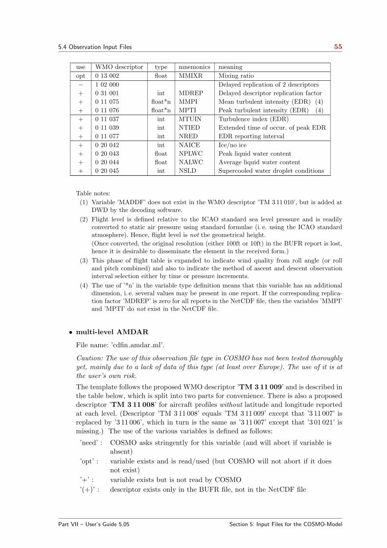
5.4 Observation Input Files 55
use WMO descriptor type mnemonics meaning
opt 0 13 002 float MMIXR Mixing ratio
− 1 02 000 Delayed replication of 2 descriptors
+ 0 31 001 int MDREP Delayed descriptor replication factor
+ 0 11 075 float*n MMPI Mean turbulent intensity (EDR) (4)
+ 0 11 076 float*n MPTI Peak turbulent intensity (EDR) (4)
+ 0 11 037 int MTUIN Turbulence index (EDR)
+ 0 11 039 int NTIED Extended time of occur. of peak EDR
+ 0 11 077 int NRED EDR reporting interval
+ 0 20 042 int NAICE Ice/no ice
+ 0 20 043 float NPLWC Peak liquid water content
+ 0 20 044 float NALWC Average liquid water content
+ 0 20 045 int NSLD Supercooled water droplet conditions
Table notes:
(1) Variable ’MADDF’ does not exist in the WMO descriptor ’TM 3 11 010’, but is added atDWD by the decoding software.
(2) Flight level is defined relative to the ICAO standard sea level pressure and is readilyconverted to static air pressure using standard formulae (i. e. using the ICAO standardatmosphere). Hence, flight level is not the geometrical height.
(Once converted, the original resolution (either 100ft or 10ft) in the BUFR report is lost,hence it is desirable to disseminate the element in the received form.)
(3) This phase of flight table is expanded to indicate wind quality from roll angle (or rolland pitch combined) and also to indicate the method of ascent and descent observationinterval selection either by time or pressure increments.
(4) The use of ’*n’ in the variable type definition means that this variable has an additionaldimension, i. e. several values may be present in one report. If the corresponding replica-tion factor ’MDREP’ is zero for all reports in the NetCDF file, then the variables ’MMPI’and ’MPTI’ do not exist in the NetCDF file.
• multi-level AMDAR
File name: ’cdfin amdar ml’.
Caution: The use of this observation file type in COSMO has not been tested thoroughlyyet, mainly due to a lack of data of this type (at least over Europe). The use of it is atthe user’s own risk.
The template follows the proposed WMO descriptor ’TM 3 11 009’ and is described inthe table below, which is split into two parts for convenience. There is also a proposeddescriptor ’TM 3 11 008’ for aircraft profiles without latitude and longitude reportedat each level. (Descriptor ’TM 3 11 008’ equals ’TM 3 11 009’ except that ’3 11 007’ isreplaced by ’3 11 006’, which in turn is the same as ’3 11 007’ except that ’3 01 021’ ismissing.) The use of the various variables is defined as follows:
’need’ : COSMO asks stringently for this variable (and will abort if variable isabsent)
’opt’ : variable exists and is read/used (but COSMO will not abort if it doesnot exist)
’+’ : variable exists but is not read by COSMO
’(+)’ : descriptor exists only in the BUFR file, not in the NetCDF file
Part VII – User’s Guide 5.05 Section 5: Input Files for the COSMO-Model
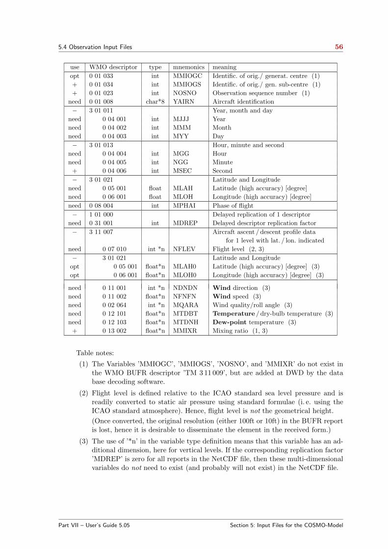
5.4 Observation Input Files 56
use WMO descriptor type mnemonics meaning
opt 0 01 033 int MMIOGC Identific. of orig./ generat. centre (1)
+ 0 01 034 int MMIOGS Identific. of orig./ gen. sub-centre (1)
+ 0 01 023 int NOSNO Observation sequence number (1)
need 0 01 008 char*8 YAIRN Aircraft identification
− 3 01 011 Year, month and day
need 0 04 001 int MJJJ Year
need 0 04 002 int MMM Month
need 0 04 003 int MYY Day
− 3 01 013 Hour, minute and second
need 0 04 004 int MGG Hour
need 0 04 005 int NGG Minute
+ 0 04 006 int MSEC Second
− 3 01 021 Latitude and Longitude
need 0 05 001 float MLAH Latitude (high accuracy) [degree]
need 0 06 001 float MLOH Longitude (high accuracy) [degree]
need 0 08 004 int MPHAI Phase of flight
− 1 01 000 Delayed replication of 1 descriptor
need 0 31 001 int MDREP Delayed descriptor replication factor
− 3 11 007 Aircraft ascent / descent profile data
for 1 level with lat. / lon. indicated
need 0 07 010 int *n NFLEV Flight level (2, 3)
− 3 01 021 Latitude and Longitude
opt 0 05 001 float*n MLAH0 Latitude (high accuracy) [degree] (3)
opt 0 06 001 float*n MLOH0 Longitude (high accuracy) [degree] (3)
need 0 11 001 int *n NDNDN Wind direction (3)
need 0 11 002 float*n NFNFN Wind speed (3)
need 0 02 064 int *n MQARA Wind quality/roll angle (3)
need 0 12 101 float*n MTDBT Temperature / dry-bulb temperature (3)
need 0 12 103 float*n MTDNH Dew-point temperature (3)
+ 0 13 002 float*n MMIXR Mixing ratio (1, 3)
Table notes:
(1) The Variables ’MMIOGC’, ’MMIOGS’, ’NOSNO’, and ’MMIXR’ do not exist inthe WMO BUFR descriptor ’TM 3 11 009’, but are added at DWD by the database decoding software.
(2) Flight level is defined relative to the ICAO standard sea level pressure and isreadily converted to static air pressure using standard formulae (i. e. using theICAO standard atmosphere). Hence, flight level is not the geometrical height.
(Once converted, the original resolution (either 100ft or 10ft) in the BUFR reportis lost, hence it is desirable to disseminate the element in the received form.)
(3) The use of ’*n’ in the variable type definition means that this variable has an ad-ditional dimension, here for vertical levels. If the corresponding replication factor’MDREP’ is zero for all reports in the NetCDF file, then these multi-dimensionalvariables do not need to exist (and probably will not exist) in the NetCDF file.
Part VII – User’s Guide 5.05 Section 5: Input Files for the COSMO-Model

5.4 Observation Input Files 57
5.4.3 Observation types without templates proposed by WMO
• ACARS
File names: ’cdfin acars’, ’cdfin acars uk’, resp. ’cdfin acars us’.
As a standard way implemented at DWD, ACARS can be read by COSMO in 2 differentways:
1. A file type (’cdfin acars us’) with BUFR obtained via GTS from ARINC Center 56(USA, denoted as ’ us’ in the table below) plus another file type (’cdfin acars uk’)with BUFR obtained via GTS from UK Met Office and Canada (denoted as ’ uk’),or
2. A single file type (’cdfin acars’) in a unified format (defined by DWD) whichcontains the reports from the two other files (denoted as ’unif.’).
The formats consist of the descriptors in the following table where
’need’: COSMO asks stringently for this variable (and will abort if variable isabsent)
’opt’: variable exists and is read/used (but COSMO will not abort if it does notexist)
’+’: variable exists but is not read by COSMO
’−’: variable does not exist in this format
unif. uk us descript. type mnemonics meaning
opt − − 0 01 033 int MMIOGC Identific. of orig./ generat. centre
+ − − 0 01 034 int MMIOGS Identific. of orig./ gen. sub-centre
need need need 0 01 008 char*8 YAIRN Aircraft identification
− + + 0 01 006 char*8 YXXNN Aircraft identification
+ − − 0 01 023 int NOSNO Observation sequence number
− − opt 0 02 001 int NIX Type of station
− − + 0 02 002 int NIW Instrument type for wind measure.
− + − 0 02 061 int NS1 Aircraft navigational system
need need need 0 05 001 float MLAH Latitude (high accuracy) [degree]
need need need 0 06 001 float MLOH Longitude (high accuracy) [deg.]
need need need 0 04 001 int MJJJ Year
need need need 0 04 002 int MMM Month
need need need 0 04 003 int MYY Day
need need need 0 04 004 int MGG Hour
need need need 0 04 005 int NGG Minute
+ − + 0 04 006 int MSEC Second
− need − 0 07 002 float MHHH Height or altit. (vert. level) (1, 2)
need − opt 0 07 004 float MPN Pressure (vertical level) (1)
− + − 0 07 007 int MH Height
need − − 0 07 010 int NFLEV Flight level (1, 2)
− − need 0 10 070 int MIAA Indicated aircraft altitude (1, 2)
opt − − 0 08 009 int NDEPF Detailed phase of flight (3)
need need need 0 11 001 int NDNDN Wind direction
need need need 0 11 002 float NFNFN Wind speed
Part VII – User’s Guide 5.05 Section 5: Input Files for the COSMO-Model
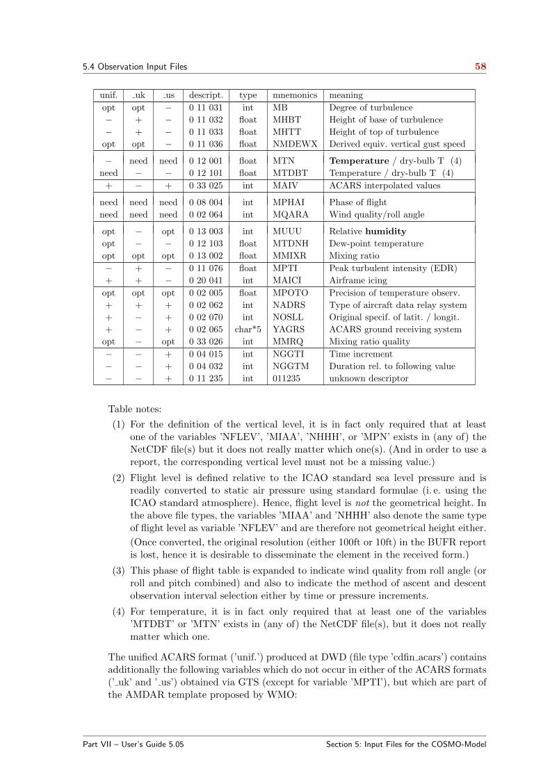
5.4 Observation Input Files 58
unif. uk us descript. type mnemonics meaning
opt opt − 0 11 031 int MB Degree of turbulence
− + − 0 11 032 float MHBT Height of base of turbulence
− + − 0 11 033 float MHTT Height of top of turbulence
opt opt − 0 11 036 float NMDEWX Derived equiv. vertical gust speed
− need need 0 12 001 float MTN Temperature / dry-bulb T (4)
need − − 0 12 101 float MTDBT Temperature / dry-bulb T (4)
+ − + 0 33 025 int MAIV ACARS interpolated values
need need need 0 08 004 int MPHAI Phase of flight
need need need 0 02 064 int MQARA Wind quality/roll angle
opt − opt 0 13 003 int MUUU Relative humidity
opt − − 0 12 103 float MTDNH Dew-point temperature
opt opt opt 0 13 002 float MMIXR Mixing ratio
− + − 0 11 076 float MPTI Peak turbulent intensity (EDR)
+ + − 0 20 041 int MAICI Airframe icing
opt opt opt 0 02 005 float MPOTO Precision of temperature observ.
+ + + 0 02 062 int NADRS Type of aircraft data relay system
+ − + 0 02 070 int NOSLL Original specif. of latit. / longit.
+ − + 0 02 065 char*5 YAGRS ACARS ground receiving system
opt − opt 0 33 026 int MMRQ Mixing ratio quality
− − + 0 04 015 int NGGTI Time increment
− − + 0 04 032 int NGGTM Duration rel. to following value
− − + 0 11 235 int 011235 unknown descriptor
Table notes:
(1) For the definition of the vertical level, it is in fact only required that at leastone of the variables ’NFLEV’, ’MIAA’, ’NHHH’, or ’MPN’ exists in (any of) theNetCDF file(s) but it does not really matter which one(s). (And in order to use areport, the corresponding vertical level must not be a missing value.)
(2) Flight level is defined relative to the ICAO standard sea level pressure and isreadily converted to static air pressure using standard formulae (i. e. using theICAO standard atmosphere). Hence, flight level is not the geometrical height. Inthe above file types, the variables ’MIAA’ and ’NHHH’ also denote the same typeof flight level as variable ’NFLEV’ and are therefore not geometrical height either.
(Once converted, the original resolution (either 100ft or 10ft) in the BUFR reportis lost, hence it is desirable to disseminate the element in the received form.)
(3) This phase of flight table is expanded to indicate wind quality from roll angle (orroll and pitch combined) and also to indicate the method of ascent and descentobservation interval selection either by time or pressure increments.
(4) For temperature, it is in fact only required that at least one of the variables’MTDBT’ or ’MTN’ exists in (any of) the NetCDF file(s), but it does not reallymatter which one.
The unified ACARS format (’unif.’) produced at DWD (file type ’cdfin acars’) containsadditionally the following variables which do not occur in either of the ACARS formats(’ uk’ and ’ us’) obtained via GTS (except for variable ’MPTI’), but which are part ofthe AMDAR template proposed by WMO:
Part VII – User’s Guide 5.05 Section 5: Input Files for the COSMO-Model

5.4 Observation Input Files 59
unif. descript. type mnemonics meaning
− 1 02 000 Delayed replication of 2 descriptors
+ 0 31 001 int MDREP Delayed descriptor replication factor
+ 0 11 075 float*n MMPI Mean turbulent intensity (EDR) (1)
+ 0 11 076 float*n MPTI Peak turbulent intensity (EDR) (1)
+ 0 11 037 int MTUIN Turbulence index (EDR)
+ 0 11 039 int NTIED Extended time of occurrence of peak EDR
+ 0 11 077 int NRED EDR reporting interval
+ 0 20 042 int NAICE Ice/no ice
+ 0 20 043 float NPLWC Peak liquid water content
+ 0 20 044 float NALWC Average liquid water content
+ 0 20 045 int NSLD Supercooled water droplet conditions
Table note:
(1) The use of ’*n’ in the variable type definition means that this variable has anadditional dimension, i. e. several values may be present in one report. If thecorresponding replication factor ’MDREP’ is zero for all reports in the NetCDFfile, then the variables ’MMPI’ and ’MPTI’ do not exist in the NetCDF file.
• Wind Profiler, RASS temperature profiler, Radar VAD wind profiles
File names: ’cdfin wprof’, ’cdfin rass’, resp. ’cdfin radar vad’.
Wind Profiler reports (’WP’), Radio Acoustic Sounding System temperature profilereports (’RASS’), and Radar Velocity Azimuth Display wind profile reports (’VAD’)are usually obtained as BUFR reports with a variety of templates. At DWD, BUFRreports with a unified template for each of the 3 data types are produced from theoriginal reports for subsequent conversion into NetCDF. These unified templates aredescribed below.
The formats consist of the descriptors in the following table where
’need’: COSMO asks stringently for this variable (and will abort if variable isabsent)
’opt’: variable exists and is read/used (but COSMO will not abort if it does notexist)
’+’: variable exists but is not read by COSMO
’−’: variable does not exist in this format
WP RASS VAD descript. type mnemonics meaning
opt opt opt 0 01 033 int MMIOGC Identif. of orig./ generat. centre
+ + + 0 01 034 int MMIOGS Identif. of orig./ gen. sub-centre
need need need 0 01 001 int MII WMO block number
need need need 0 01 002 int NIII WMO station number
+ + − 0 02 001 int NIX Type of station
need need need 0 04 001 int MJJJ Year
need need need 0 04 002 int MMM Month
need need need 0 04 003 int MYY Day
need need need 0 04 004 int MGG Hour
need need need 0 04 005 int NGG Minute
Part VII – User’s Guide 5.05 Section 5: Input Files for the COSMO-Model
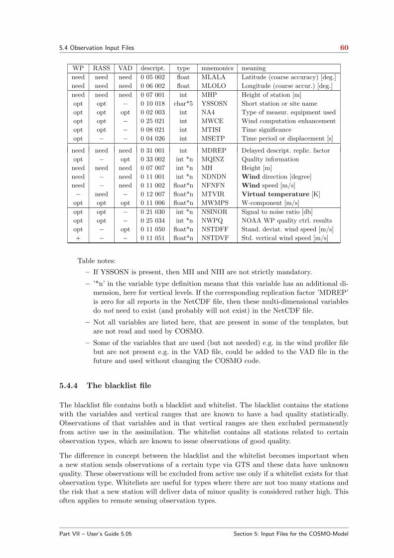
5.4 Observation Input Files 60
WP RASS VAD descript. type mnemonics meaning
need need need 0 05 002 float MLALA Latitude (coarse accuracy) [deg.]
need need need 0 06 002 float MLOLO Longitude (coarse accur.) [deg.]
need need need 0 07 001 int MHP Height of station [m]
opt opt − 0 10 018 char*5 YSSOSN Short station or site name
opt opt opt 0 02 003 int NA4 Type of measur. equipment used
opt opt − 0 25 021 int MWCE Wind computation enhancement
opt opt − 0 08 021 int MTISI Time significance
opt − − 0 04 026 int MSETP Time period or displacement [s]
need need need 0 31 001 int MDREP Delayed descript. replic. factor
opt − opt 0 33 002 int *n MQINZ Quality information
need need need 0 07 007 int *n MH Height [m]
need − need 0 11 001 int *n NDNDN Wind direction [degree]
need − need 0 11 002 float*n NFNFN Wind speed [m/s]
− need − 0 12 007 float*n MTVIR Virtual temperature [K]
opt opt opt 0 11 006 float*n MWMPS W-component [m/s]
opt opt − 0 21 030 int *n NSINOR Signal to noise ratio [db]
opt opt − 0 25 034 int *n NWPQ NOAA WP quality ctrl. results
opt − opt 0 11 050 float*n NSTDFF Stand. deviat. wind speed [m/s]
+ − − 0 11 051 float*n NSTDVF Std. vertical wind speed [m/s]
Table notes:
– If YSSOSN is present, then MII and NIII are not strictly mandatory.
– ’*n’ in the variable type definition means that this variable has an additional di-mension, here for vertical levels. If the corresponding replication factor ’MDREP’is zero for all reports in the NetCDF file, then these multi-dimensional variablesdo not need to exist (and probably will not exist) in the NetCDF file.
– Not all variables are listed here, that are present in some of the templates, butare not read and used by COSMO.
– Some of the variables that are used (but not needed) e.g. in the wind profiler filebut are not present e.g. in the VAD file, could be added to the VAD file in thefuture and used without changing the COSMO code.
5.4.4 The blacklist file
The blacklist file contains both a blacklist and whitelist. The blacklist contains the stationswith the variables and vertical ranges that are known to have a bad quality statistically.Observations of that variables and in that vertical ranges are then excluded permanentlyfrom active use in the assimilation. The whitelist contains all stations related to certainobservation types, which are known to issue observations of good quality.
The difference in concept between the blacklist and the whitelist becomes important whena new station sends observations of a certain type via GTS and these data have unknownquality. These observations will be excluded from active use only if a whitelist exists for thatobservation type. Whitelists are useful for types where there are not too many stations andthe risk that a new station will deliver data of minor quality is considered rather high. Thisoften applies to remote sensing observation types.
Part VII – User’s Guide 5.05 Section 5: Input Files for the COSMO-Model
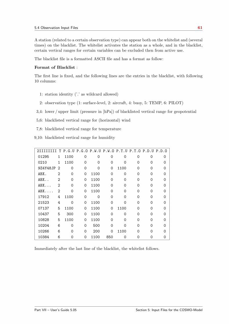
5.4 Observation Input Files 61
A station (related to a certain observation type) can appear both on the whitelist and (severaltimes) on the blacklist. The whitelist activates the station as a whole, and in the blacklist,certain vertical ranges for certain variables can be excluded then from active use.
The blacklist file is a formatted ASCII file and has a format as follow:
Format of Blacklist :
The first line is fixed, and the following lines are the entries in the blacklist, with following10 columns:
1: station identity (’.’ as wildcard allowed)
2: observation type (1: surface-level, 2: aircraft, 4: buoy, 5: TEMP, 6: PILOT)
3,4: lower / upper limit (pressure in [hPa]) of blacklisted vertical range for geopotential
5,6: blacklisted vertical range for (horizontal) wind
7,8: blacklisted vertical range for temperature
9,10: blacklisted vertical range for humidity
2IIIIIIII T P.G.U P.G.O P.W.U P.W.O P.T.U P.T.O P.D.U P.D.O
01295 1 1100 0 0 0 0 0 0 0
0210 1 1100 0 0 0 0 0 0 0
9Z4Y48JP 2 0 0 0 0 1100 0 0 0
ABX. 2 0 0 1100 0 0 0 0 0
ABX.. 2 0 0 1100 0 0 0 0 0
ABX... 2 0 0 1100 0 0 0 0 0
ABX.... 2 0 0 1100 0 0 0 0 0
17912 4 1100 0 0 0 0 0 0 0
21523 4 0 0 1100 0 0 0 0 0
07137 5 1100 0 1100 0 1100 0 0 0
10437 5 300 0 1100 0 0 0 0 0
10828 5 1100 0 1100 0 0 0 0 0
10204 6 0 0 500 0 0 0 0 0
10266 6 0 0 200 0 1100 0 0 0
10384 6 0 0 1100 850 0 0 0 0
Immediately after the last line of the blacklist, the whitelist follows.
Part VII – User’s Guide 5.05 Section 5: Input Files for the COSMO-Model

5.4 Observation Input Files 62
Standard format of Whitelist Alternative format of Whitelist
WHITELIST
03019 6 132
10135 6 132
10266 6 132
10394 6 132
47912 6 134
47945 6 134
72246 6 136
74341 6 136
10169 6 137
10204 6 137
10384 6 137
WHITELIST 6 132
03019 6 132
10135 6 132
10266 6 132
10394 6 132
WHITELIST 6 133
WHITELIST 6 134
47912 6 134
47945 6 134
WHITELIST 6 136
72246 6 136
74341 6 136
WHITELIST 6 137
10169 6 137
10204 6 137
10384 6 137
In the standard format, the first line is fixed, and the following lines are the entries in thewhitelist, with the following 3 columns:
1: station identity
2: observation type (currently only 6: PILOT , which includes profilers)
3: observation code type (132: European wind profiler,
133: European RASS / SODAR,
134: Japan. wind profiler / RASS,
136: US wind profiler / RASS,
137: Radar VAD wind profiles)
The standard format assumes a whitelist exactly for those observation code types for whichthere are entries on whitelist. In the blacklist file used at DWD currently, no RASS profilerstation is on the whitelist, which implies that COSMO will assume that no whitelist existsfor RASS. Hence, all RASS reports would be used actively unless they are on the blacklist.This is indeed the case, i. e. the temperature profiles from all the known RASS stations areput on the blacklist, see e. g. station 10266 in the example above.
There is an alternative format for the whitelist which can be used (but is not yet as thoroughlytested). A line containing ’WHITELIST’ and observation type and code type precedes thewhitelist for each code type, even if the whitelist for that code type is empty. Only thisalternative format allows to use empty whitelists, and the above example in this alternativeformat is also shown above.
Part VII – User’s Guide 5.05 Section 5: Input Files for the COSMO-Model

63
Section 6
Namelist Input for COSMO-Model
The execution of the COSMO-Model is controlled by 14 NAMELIST-groups:
- LMGRID – specifying the domain and the size of the grid
- RUNCTL – parameters for the model run
- DYNCTL – parameters for the adiabatic model
- PHYCTL – parameters for the diabatic model
- TUNING – parameters for tuning dynamics and physics
- DIACTL – parameters for the diagnostic calculations
- SATCTL – parameters for the satellite images
- INICTL – parameters for the initialization of model variables
- EPSCTL – controlling the ensemble prediction mode
- IOCTL – controlling the environment
- DATABASE – specification of database job
- GRIBIN – controlling the grib input
- GRIBOUT – controlling the grib output
- NUDGING – controlling the data assimilation
These NAMELIST-groups have to appear in the corresponding INPUT * files. See Tab. 5.1 forthe distribution of the NAMELIST-groups to the INPUT * files. The INPUT * files have to be inthe directory, from where the model is started. Every group is read in a special subroutinecalled input groupname. This subroutine also sets default values for all parameters andchecks most parameters that have been changed for correctness and consistency.
The NAMELIST variables can be specified by the user in the run-script for the model, whichthen creates the INPUT * files. An excerpt of this run script is shown in Figure 6.1 for theforecast part and in Figure 7.1 for the nudging part.
Part VII – User’s Guide 5.05 Section 6: Namelist Input for COSMO-Model
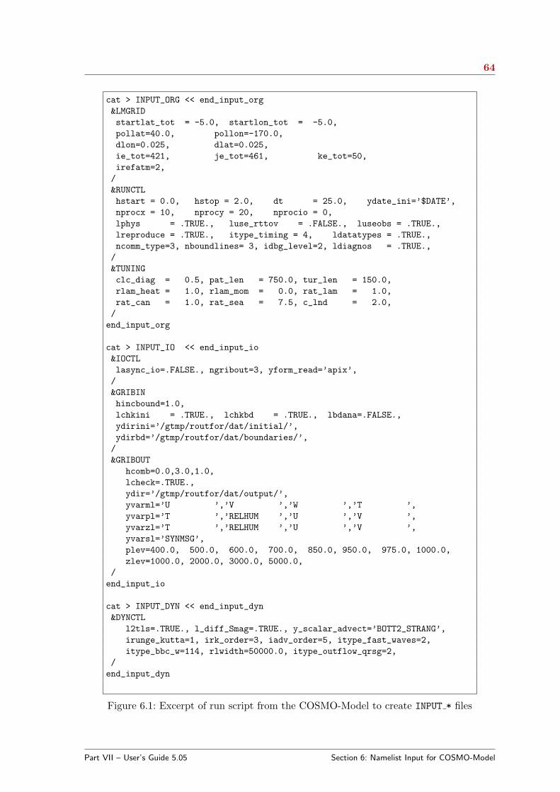
64
cat > INPUT_ORG << end_input_org
&LMGRID
startlat_tot = -5.0, startlon_tot = -5.0,
pollat=40.0, pollon=-170.0,
dlon=0.025, dlat=0.025,
ie_tot=421, je_tot=461, ke_tot=50,
irefatm=2,
/
&RUNCTL
hstart = 0.0, hstop = 2.0, dt = 25.0, ydate_ini=’$DATE’,
nprocx = 10, nprocy = 20, nprocio = 0,
lphys = .TRUE., luse_rttov = .FALSE., luseobs = .TRUE.,
lreproduce = .TRUE., itype_timing = 4, ldatatypes = .TRUE.,
ncomm_type=3, nboundlines= 3, idbg_level=2, ldiagnos = .TRUE.,
/
&TUNING
clc_diag = 0.5, pat_len = 750.0, tur_len = 150.0,
rlam_heat = 1.0, rlam_mom = 0.0, rat_lam = 1.0,
rat_can = 1.0, rat_sea = 7.5, c_lnd = 2.0,
/
end_input_org
cat > INPUT_IO << end_input_io
&IOCTL
lasync_io=.FALSE., ngribout=3, yform_read=’apix’,
/
&GRIBIN
hincbound=1.0,
lchkini = .TRUE., lchkbd = .TRUE., lbdana=.FALSE.,
ydirini=’/gtmp/routfor/dat/initial/’,
ydirbd=’/gtmp/routfor/dat/boundaries/’,
/
&GRIBOUT
hcomb=0.0,3.0,1.0,
lcheck=.TRUE.,
ydir=’/gtmp/routfor/dat/output/’,
yvarml=’U ’,’V ’,’W ’,’T ’,
yvarpl=’T ’,’RELHUM ’,’U ’,’V ’,
yvarzl=’T ’,’RELHUM ’,’U ’,’V ’,
yvarsl=’SYNMSG’,
plev=400.0, 500.0, 600.0, 700.0, 850.0, 950.0, 975.0, 1000.0,
zlev=1000.0, 2000.0, 3000.0, 5000.0,
/
end_input_io
cat > INPUT_DYN << end_input_dyn
&DYNCTL
l2tls=.TRUE., l_diff_Smag=.TRUE., y_scalar_advect=’BOTT2_STRANG’,
irunge_kutta=1, irk_order=3, iadv_order=5, itype_fast_waves=2,
itype_bbc_w=114, rlwidth=50000.0, itype_outflow_qrsg=2,
/
end_input_dyn
Figure 6.1: Excerpt of run script from the COSMO-Model to create INPUT * files
Part VII – User’s Guide 5.05 Section 6: Namelist Input for COSMO-Model
65
The following sections serve as a complete reference to all namelist variables used in theCOSMO-Model. There is a section for every namelist group. Within the sections the de-scriptions of the variables is organized in subgroups, if the variables can be separated intodifferent scopes. For example in the physics group PHYCTL there is a subgroup for every pa-rameterization. All variables are displayed in tables, showing the name of the variable, theirnumerical type in the model, the definition including some comments and the default value.
A problem that less experienced COSMO users often face, is to find out, which namelistvariables they have to adapt, if they want to change e.g. the domain or the resolution of
their application. Therefore we introduced an additional 5th column to the tables, whichshould indicate the dependency of a variable on a special category. The following categorieshave been defined up to now:
M: Mode of simulation (NWP, CLM, ITC, ART)
R: Region
dx: Horizontal resolution
dz: Vertical resolution
dt: Time step
BC: Boundary conditions
P: Performance
If you want to change for example your horizontal resolution, you should check for whichvariables a dependency on dx is listed in the tables below.
Part VII – User’s Guide 5.05 Section 6: Namelist Input for COSMO-Model
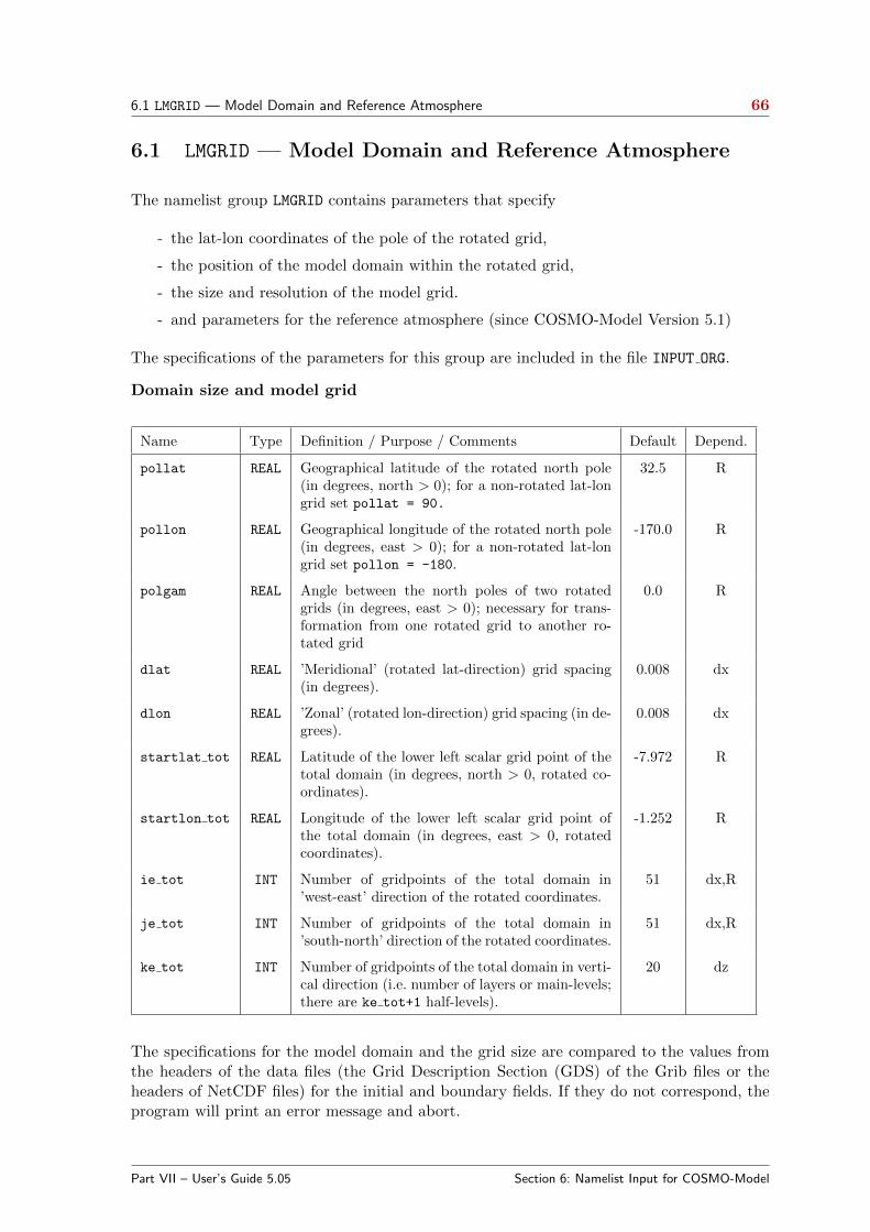
6.1 LMGRID — Model Domain and Reference Atmosphere 66
6.1 LMGRID — Model Domain and Reference Atmosphere
The namelist group LMGRID contains parameters that specify
- the lat-lon coordinates of the pole of the rotated grid,
- the position of the model domain within the rotated grid,
- the size and resolution of the model grid.
- and parameters for the reference atmosphere (since COSMO-Model Version 5.1)
The specifications of the parameters for this group are included in the file INPUT ORG.
Domain size and model grid
Name Type Definition / Purpose / Comments Default Depend.
pollat REAL Geographical latitude of the rotated north pole(in degrees, north > 0); for a non-rotated lat-longrid set pollat = 90.
32.5 R
pollon REAL Geographical longitude of the rotated north pole(in degrees, east > 0); for a non-rotated lat-longrid set pollon = -180.
-170.0 R
polgam REAL Angle between the north poles of two rotatedgrids (in degrees, east > 0); necessary for trans-formation from one rotated grid to another ro-tated grid
0.0 R
dlat REAL ’Meridional’ (rotated lat-direction) grid spacing(in degrees).
0.008 dx
dlon REAL ’Zonal’ (rotated lon-direction) grid spacing (in de-grees).
0.008 dx
startlat tot REAL Latitude of the lower left scalar grid point of thetotal domain (in degrees, north > 0, rotated co-ordinates).
-7.972 R
startlon tot REAL Longitude of the lower left scalar grid point ofthe total domain (in degrees, east > 0, rotatedcoordinates).
-1.252 R
ie tot INT Number of gridpoints of the total domain in’west-east’ direction of the rotated coordinates.
51 dx,R
je tot INT Number of gridpoints of the total domain in’south-north’ direction of the rotated coordinates.
51 dx,R
ke tot INT Number of gridpoints of the total domain in verti-cal direction (i.e. number of layers or main-levels;there are ke tot+1 half-levels).
20 dz
The specifications for the model domain and the grid size are compared to the values fromthe headers of the data files (the Grid Description Section (GDS) of the Grib files or theheaders of NetCDF files) for the initial and boundary fields. If they do not correspond, theprogram will print an error message and abort.
Part VII – User’s Guide 5.05 Section 6: Namelist Input for COSMO-Model

6.1 LMGRID — Model Domain and Reference Atmosphere 67
Variables for the reference atmosphere
Since Version 5.1, there are also namelist variables to specify the reference atmosphere pa-rameters, because these parameters cannot be written to the GRIB2 meta data any more.
When using GRIB1 or NetCDF, these parameters are specified in INT2LM and are written tothe meta data of all atmospheric fields. The pressure field exchanged between INT2LM andthe COSMO-Model or within a COSMO-Model assimilation cycle is the pressure deviationPP, because this field suffers less from the precision loss due to GRIB packing than the fullpressure P. When the COSMO-Model reads the atmospheric fields, including PP, it gets thevalues for the reference atmosphere from the meta data, constructs the reference pressurefield P0 and then computes the full pressure P.
When using GRIB2, not the pressure deviation, but the full pressure field P is exchangedbetween INT2LM and the COSMO-Model or within a COSMO-Model assimilation cycle.This is done using a packing to 24 bits (while most other fields are packed to 16 bits). Thisgives a high enough precision for the values of the full pressure. Internally, the COSMO-Modelis working with the pressure deviation as a prognostic variable, therefore it has to compute thereference pressure field P0, and for that has to know the reference atmosphere parameters.Therefore we introduced the following namelist variables; their names and meanings areidentical to the corresponding namelist variables in the INT2LM.
Name Type Definition / Purpose / Comments Default Depend.
irefatm INT type of reference atmosphere
1: The reference atmosphere is based on aconstant rate β for the temperature in-crease with the logarithm of pressure:∂T0/∂ ln p0 = β.
2: The reference atmosphere is based on atemperature profile
t0(z) = (t0sl −∆t) + ∆t · exp
(−zhscal
),
where z = hhl(k) is the height of a modelgrid point. If this option is used, the valuesfor ∆t = delta t and hscal = h scal havealso to be set.
2 dz
p0sl REAL constant reference pressure on sea-level 10000.0
t0sl REAL constant reference temperature on sea-level 288.15
dt0lp REAL d (t0) / d (ln p0) 42.0
delta t REAL temperature difference between sea level andstratosphere (for irefatm=2)
75.0
h scal REAL scale height (for irefatm=2) 10000.0
Note that the reference atmosphere used in INT2LM and the one used in the COSMO-Model need not be the same, when the full pressure P is exchanged. The only dependencyis: If the top of the atmosphere is above 27 km and INT2LM is using irefatm=2, then alsothe COSMO-Model has to use irefatm=2.
Part VII – User’s Guide 5.05 Section 6: Namelist Input for COSMO-Model
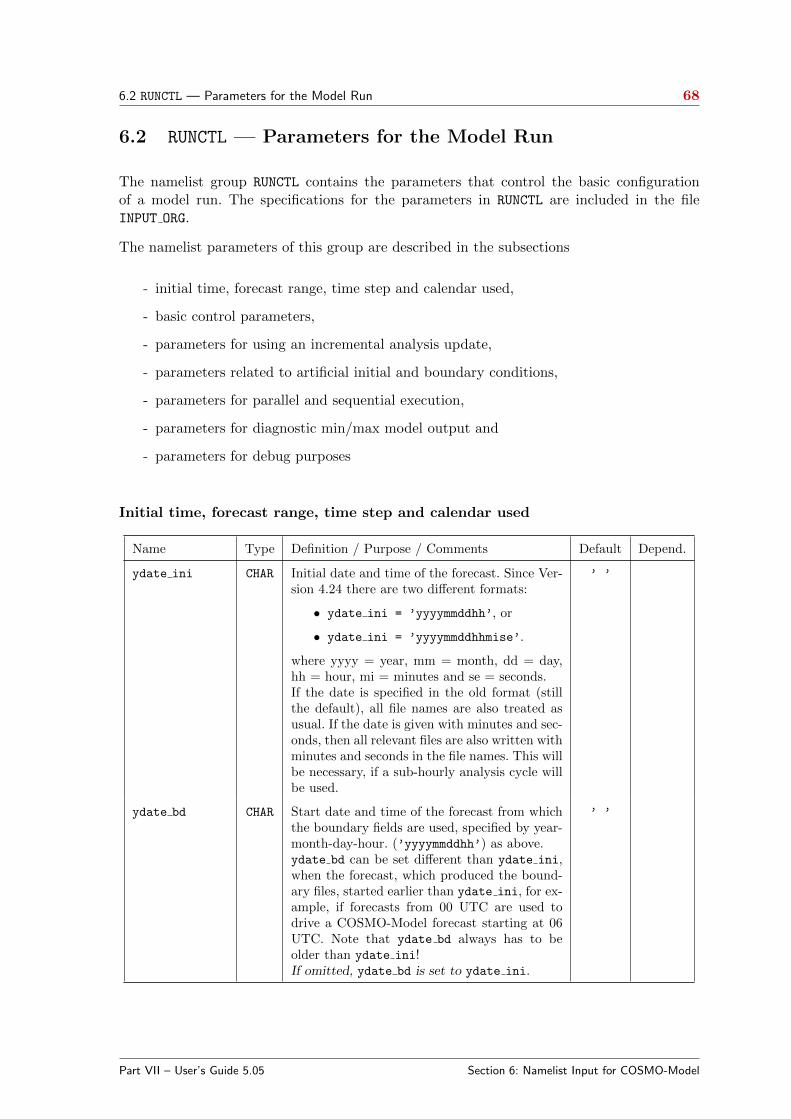
6.2 RUNCTL — Parameters for the Model Run 68
6.2 RUNCTL — Parameters for the Model Run
The namelist group RUNCTL contains the parameters that control the basic configurationof a model run. The specifications for the parameters in RUNCTL are included in the fileINPUT ORG.
The namelist parameters of this group are described in the subsections
- initial time, forecast range, time step and calendar used,
- basic control parameters,
- parameters for using an incremental analysis update,
- parameters related to artificial initial and boundary conditions,
- parameters for parallel and sequential execution,
- parameters for diagnostic min/max model output and
- parameters for debug purposes
Initial time, forecast range, time step and calendar used
Name Type Definition / Purpose / Comments Default Depend.
ydate ini CHAR Initial date and time of the forecast. Since Ver-sion 4.24 there are two different formats:
• ydate ini = ’yyyymmddhh’, or
• ydate ini = ’yyyymmddhhmise’.
where yyyy = year, mm = month, dd = day,hh = hour, mi = minutes and se = seconds.If the date is specified in the old format (stillthe default), all file names are also treated asusual. If the date is given with minutes and sec-onds, then all relevant files are also written withminutes and seconds in the file names. This willbe necessary, if a sub-hourly analysis cycle willbe used.
’ ’
ydate bd CHAR Start date and time of the forecast from whichthe boundary fields are used, specified by year-month-day-hour. (’yyyymmddhh’) as above.ydate bd can be set different than ydate ini,when the forecast, which produced the bound-ary files, started earlier than ydate ini, for ex-ample, if forecasts from 00 UTC are used todrive a COSMO-Model forecast starting at 06UTC. Note that ydate bd always has to beolder than ydate ini!If omitted, ydate bd is set to ydate ini.
’ ’
Part VII – User’s Guide 5.05 Section 6: Namelist Input for COSMO-Model
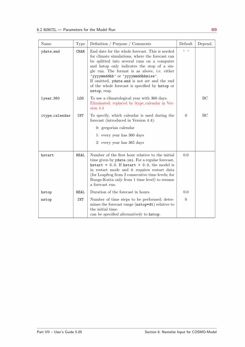
6.2 RUNCTL — Parameters for the Model Run 69
Name Type Definition / Purpose / Comments Default Depend.
ydate end CHAR End date for the whole forecast. This is neededfor climate simulations, where the forecast canbe splitted into several runs on a computerand hstop only indicates the stop of a sin-gle run. The format is as above, i.e. either’yyyymmddhh’ or ’yyyymmddhhmise’.If omitted, ydate end is not set and the endof the whole forecast is specified by hstop ornstop, resp.
’ ’
lyear 360 LOG To use a climatological year with 360 days.Eliminated: replaced by itype calendar in Ver-sion 4.4
BC
itype calendar INT To specify, which calendar is used during theforecast (introduced in Version 4.4):
0: gregorian calendar
1: every year has 360 days
2: every year has 365 days
0 BC
hstart REAL Number of the first hour relative to the initialtime given by ydate ini. For a regular forecast,hstart = 0.0. If hstart > 0.0, the model isin restart mode and it requires restart data(for Leapfrog from 2 consecutive time levels; forRunge-Kutta only from 1 time level) to resumea forecast run.
0.0
hstop REAL Duration of the forecast in hours. 0.0
nstop INT Number of time steps to be performed; deter-mines the forecast range (nstop*dt) relative tothe initial time.can be specified alternatively to hstop.
0
Part VII – User’s Guide 5.05 Section 6: Namelist Input for COSMO-Model
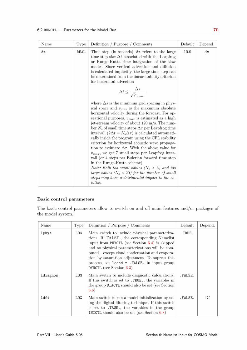
6.2 RUNCTL — Parameters for the Model Run 70
Name Type Definition / Purpose / Comments Default Depend.
dt REAL Time step (in seconds); dt refers to the largetime step size ∆t associated with the Leapfrogor Runge-Kutta time integration of the slowmodes. Since vertical advection and diffusionis calculated implicitly, the large time step canbe determined from the linear stability criterionfor horizontal advection
∆t ≤ ∆s√2 vmax
,
where ∆s is the minimum grid spacing in phys-ical space and vmax is the maximum absolutehorizontal velocity during the forecast. For op-erational purposes, vmax is estimated as a highjet-stream velocity of about 120 m/s. The num-berNs of small time steps ∆τ per Leapfrog timeintervall (2∆t = Ns∆τ) is calculated automati-cally inside the program using the CFL stabilitycriterion for horizontal acoustic wave propaga-tion to estimate ∆τ . With the above value forvmax, we get 7 small steps per Leapfrog inter-vall (or 4 steps per Eulerian forward time stepin the Runge-Kutta scheme).Note: Both too small values (Ns < 3) and toolarge values (Ns > 20) for the number of smallsteps may have a detrimental impact to the so-lution.
10.0 dx
Basic control parameters
The basic control parameters allow to switch on and off main features and/or packages ofthe model system.
Name Type Definition / Purpose / Comments Default Depend.
lphys LOG Main switch to include physical parameteriza-tions. If .FALSE., the corresponding Namelistinput from PHYCTL (see Section 6.4) is skippedand no physical parameterizations will be com-puted – except cloud condensation and evapora-tion by saturation adjustment. To supress thisprocess, set lcond = .FALSE. in input groupDYNCTL (see Section 6.3).
.TRUE.
ldiagnos LOG Main switch to include diagnostic calculations.If this switch is set to .TRUE., the variables inthe group DIACTL should also be set (see Section6.6)
.FALSE.
ldfi LOG Main switch to run a model initialization by us-ing the digital filtering technique. If this switchis set to .TRUE., the variables in the groupINICTL should also be set (see Section 6.8)
.FALSE. IC
Part VII – User’s Guide 5.05 Section 6: Namelist Input for COSMO-Model
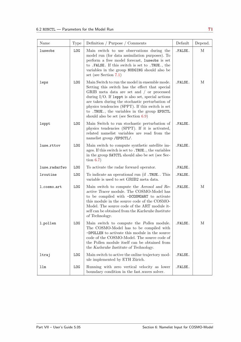
6.2 RUNCTL — Parameters for the Model Run 71
Name Type Definition / Purpose / Comments Default Depend.
luseobs LOG Main switch to use observations during themodel run (for data assimilation purposes). Toperform a free model forecast, luseobs is setto .FALSE. If this switch is set to .TRUE., thevariables in the group NUDGING should also beset (see Section 7.1)
.FALSE. M
leps LOG Main Switch to run the model in ensemble mode.Setting this switch has the effect that specialGRIB meta data are set and / or processedduring I/O. If lsppt is also set, special actionsare taken during the stochastic perturbation ofphysics tendencies (SPPT). If this switch is setto .TRUE., the variables in the group EPSCTL
should also be set (see Section 6.9)
.FALSE. M
lsppt LOG Main Switch to run stochastic perturbation ofphysics tendencies (SPPT). If it is activated,related namelist variables are read from thenamelist group /EPSCTL/.
.FALSE.
luse rttov LOG Main switch to compute synthetic satellite im-ages. If this switch is set to .TRUE., the variablesin the group SATCTL should also be set (see Sec-tion 6.7)
.FALSE.
luse radarfwo LOG To activate the radar forward operator. .FALSE.
lroutine LOG To indicate an operational run (if .TRUE.. Thisvariable is used to set GRIB2 meta data.
.FALSE.
l cosmo art LOG Main switch to compute the Aerosol and Re-active Tracer module. The COSMO-Model hasto be compiled with -DCOSMOART to activatethis module in the source code of the COSMO-Model. The source code of the ART module it-self can be obtained from the Karlsruhe Instituteof Technology.
.FALSE. M
l pollen LOG Main switch to compute the Pollen module.The COSMO-Model has to be compiled with-DPOLLEN to activate this module in the sourcecode of the COSMO-Model. The source code ofthe Pollen module itself can be obtained fromthe Karlsruhe Institute of Technology.
.FALSE. M
ltraj LOG Main switch to active the online trajectory mod-ule implemented by ETH Zurich.
.FALSE.
llm LOG Running with zero vertical velocity as lowerboundary condition in the fast waves solver.
.FALSE.
Part VII – User’s Guide 5.05 Section 6: Namelist Input for COSMO-Model

6.2 RUNCTL — Parameters for the Model Run 72
Parameters for the blocked physics
With the implementation of the unified COSMO-ICON physical parameterizations there isthe need for a special data structure in the physics, because ICON uses a 2-dimensional datastructure with (number of grid points, vertical dimension).
This data format, which is called the blocked data format, has now been implemented in theCOSMO-Model (starting in Version 5.01). A special copy-in / copy-out mechanism hasbeen implemented to copy data between this new blocked structure and the basic 3-D dataformat of the COSMO-Model.
In an ideal world it is:
nproma · nblock = (iendpar - istartpar + 1) · jendpar - jstartpar + 1,
where nproma is the number of grid points and nblock is the number of blocks necessary tohold all grid points from the original COSMO 2-D data structure (ie,je). And because theworld never is ideal, the last block will usually have a shorter length than nproma. In theprogram this length is denoted with nlastproma.
To specify the blocked data structure one can either specify the length of the first dimen-sion, nproma, or the number of blocks nblock. In the COSMO-Model we implemented bothvariables as namelist variables, but specifying nblock has precedence over specifying nproma.
Name Type Definition / Purpose / Comments Default
nproma INT To specify the number of grid points within one block of theblocked data structure.(Introduced in Version 5.01).
16
nblock INT To specify the number of blocks of the blocked data structure.(Introduced in Version 5.01).
-1
Part VII – User’s Guide 5.05 Section 6: Namelist Input for COSMO-Model

6.2 RUNCTL — Parameters for the Model Run 73
Parameters for using an incremental analysis update
Usually the model is started from an analysis file. When using the incremental analysisupdate (IAU), the model is started from a first guess (a forecast with lead time given bythe namelist variable nsec fg (in namelist group /GRIBIN/. The analysis increments areadded to the model fields incrementally at each time step during the model integration overa certain period, given by namelist variable peri iau.
Further details:
• The IAU updates the sum of water vapour and cloud water. After this, the watervapour and cloud water are balanced without applying any latent heating because theIAU updates reflect corrections due to observations and not due to simulated physicalprocesses.
• Clipping is performed for all the other variables with zero lower bound (except forthose related to temperature).
• In the case of the two-moment microphysics, the number concentrations of the hy-drometeors are adjusted in order to preserve the particle size distributions. For zeroprior hydrometeor contents and hence undefined prior number concentrations, the newconcentrations are set consistent with assumptions in the Seifert/Beheng two-momentscheme.
• The IAU is not applied to the variables related to the snow cover and sea ice analyses fortwo reasons. Firstly, they have only an indirect influence on the atmospheric balancevia the surface fluxes. Secondly, the analysis values and increments of ice and snowtemperature and snow densitiy are not well defined in case of missing ice / snow in theanalysis or first guess.
Name Type Definition / Purpose / Comments Default
itype iau INT To select the type of incremental analysis update (IAU):
0: no IAU is done (default)
1: IAU for all variables (except rel. to snow cover, sea ice)
2: IAU except for QR, QS, QI, QG, snow cover, sea ice
(Introduced in Version 5.04d).
0
peri iau REAL Period [s] over which IAU is applied.(Introduced in Version 5.04d).
3600.0
Part VII – User’s Guide 5.05 Section 6: Namelist Input for COSMO-Model

6.2 RUNCTL — Parameters for the Model Run 74
Parameters related to artificial initial and boundary conditions
The following parameters are only in effect if the control parameter lartif data is set to.TRUE.. This parameter controls the basic type of the simulation: if it is set to .TRUE.,a runwith artificial (or idealized) initial and boundary data is performed. If it is set to .FALSE., areal-case simulation with initial and boundary data coming from a coarse-grid driving modelor from an assimilation run is done.
If lartif data=.TRUE. is chosen, there are parameters to control the type of lateral bound-ary conditions (relaxation, periodic, open) and to include/exclude metrical terms. Also, inthis case another namelist ARTIFCTL will be read from the file INPUT IDEAL and the namelistGRIBIN from file INPUT IO has no effect and will be skipped. ARTIFCTL offers parameters fora wide variety of choices to configure idealized runs, such as definition of orography (ideal-ized hills or pre user-provided ASCII files), specification of atmospheric and soil profiles forintitial and boundary conditions, and artificial convection triggers (warm bubbles, soil hotspots).
Name Type Definition / Purpose / Comments Default Depend.
lartif data LOG If .TRUE., the model runs with user-defined ini-tial and boundary data. All Namelist input fromGRIBIN is skipped and the corresponding param-eters are not in effect. A Namelist group /AR-TIFCTL/ has to be defined instead.If .FALSE., the model expects initial and boundarydata in Grib or NetCDF format. Control parame-ters for these files are contained in Namelist inputgroup GRIBIN.(lartif data has been renamed (named lgen be-fore) and moved from group GRIBIN to RUNCTL inVersion 4.8.)
.FALSE. M
l2dim LOG Run a 2-dimensional model version.To run the model in 2-d mode, the number ofgridpoints in south-north direction must be set toje tot = 5.
.FALSE. M
lperi LOG Eliminated in Version 4.17 and replaced bylperi x and lperi y (see below).
-
lperi x LOG Use periodic lateral boundary conditions in x-direction.
.FALSE.
lperi y LOG Use periodic lateral boundary conditions in y-direction.
.FALSE.
lcori LOG moved to group /DYNCTL/ in Version 4.8
lmetr LOG moved to group /DYNCTL/ in Version 4.8
lradlbc LOG moved to group /DYNCTL/ in Version 4.8
Also, a 1-dimensional set-up can be realized by setting the number of gridpoints in west-eastdirection to ie tot = 5 and choosing periodic lateral boundary conditions. Depending onthe problem at hand, however, some additional modification of the dynamics code might beneccessary (e.g. to include a constant pressure gradient in terms of a geostrophic wind).
Part VII – User’s Guide 5.05 Section 6: Namelist Input for COSMO-Model

6.2 RUNCTL — Parameters for the Model Run 75
Note:To generate artificial initial and boundary conditions for idealized model runs, the routinesgen ini data (to specify initial data) and gen bound data (to specify boundary data) con-tained in the source file src artifdata.f90 are used. The configuration of such idealizedmodel runs can be done with the help of a large number of namelist parameters in thenamelist ARTIFCTL in the file INPUT IDEAL, which offers a wide variety of choices for orogra-phy, atmosphere and soil profiles for initial and boundary conditions and convection triggers.However, there is no unique way for this specification as it depends on the problem to beconsidered, and therefore it is possible to extend src artifdata.f90 according to specialneeds.
The documentation of the namelist group ARTIFCTL would go beyond the scope of this UserGuide, therefore an extra document will be provided for running idealized cases.
Parameters for parallel and sequential execution
This section contains parameters for the decomposition (parallelization) of the model domainand for generating additional information about timings for the different parts of the modelrun. Furthermore, the type of communication can be specified (see parameters ldatatypes,ncomm type). How the different types of communications perform surely depends on thecomputer used. Therefore it would require some testing to find the optimal settings.
Name Type Definition / Purpose / Comments Default Depend.
nprocx INT Number of processors in the x-direction of thegrid.
1 P
nprocy INT Number of processors in the y-direction of thegrid.
1 P
nprocio INT Number of processors for GRIB I/O. 0 P
num asynio comm INT To choose the number of asynchronous I/Ocommunicators for NetCDF. With severalcommunicators it is possible to parallelizethe output over the files to be written (theGRIBOUT namelists), so that several outputfiles can be written simultaneously.
0 P
num iope percomm INT To choose the number of asynchronous I/Oprocesses per communicator for NetCDF I/O.With several processes per communicator itis possible to do a parallel writing of sin-gle files. This is only possible, if the parallelNetCDF library is available and the code hasbeen compiled with the preprocessor directive-DPNETCDF.
0 P
Part VII – User’s Guide 5.05 Section 6: Namelist Input for COSMO-Model
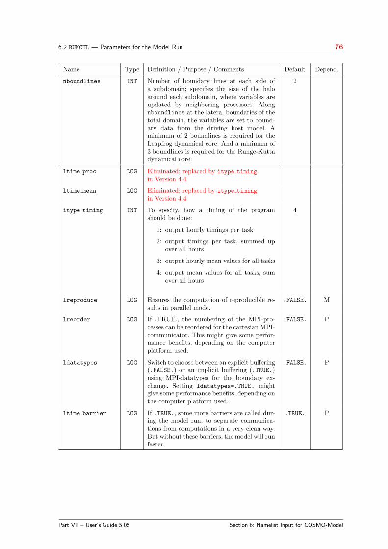
6.2 RUNCTL — Parameters for the Model Run 76
Name Type Definition / Purpose / Comments Default Depend.
nboundlines INT Number of boundary lines at each side ofa subdomain; specifies the size of the haloaround each subdomain, where variables areupdated by neighboring processors. Alongnboundlines at the lateral boundaries of thetotal domain, the variables are set to bound-ary data from the driving host model. Aminimum of 2 boundlines is required for theLeapfrog dynamical core. And a minimum of3 boundlines is required for the Runge-Kuttadynamical core.
2
ltime proc LOG Eliminated; replaced by itype timing
in Version 4.4
ltime mean LOG Eliminated; replaced by itype timing
in Version 4.4
itype timing INT To specify, how a timing of the programshould be done:
1: output hourly timings per task
2: output timings per task, summed upover all hours
3: output hourly mean values for all tasks
4: output mean values for all tasks, sumover all hours
4
lreproduce LOG Ensures the computation of reproducible re-sults in parallel mode.
.FALSE. M
lreorder LOG If .TRUE., the numbering of the MPI-pro-cesses can be reordered for the cartesian MPI-communicator. This might give some perfor-mance benefits, depending on the computerplatform used.
.FALSE. P
ldatatypes LOG Switch to choose between an explicit buffering(.FALSE.) or an implicit buffering (.TRUE.)using MPI-datatypes for the boundary ex-change. Setting ldatatypes=.TRUE. mightgive some performance benefits, depending onthe computer platform used.
.FALSE. P
ltime barrier LOG If .TRUE., some more barriers are called dur-ing the model run, to separate communica-tions from computations in a very clean way.But without these barriers, the model will runfaster.
.TRUE. P
Part VII – User’s Guide 5.05 Section 6: Namelist Input for COSMO-Model

6.2 RUNCTL — Parameters for the Model Run 77
Name Type Definition / Purpose / Comments Default Depend.
ncomm type INT To choose a certain type of communication:
1: immediate send, blocking receive andwait on the sender side
2: immediate receive, blocking send andwait on the receiver side
3: using MPI SENDRECV
1
Parameters for diagnostic min/max model output
Name Type Definition / Purpose / Comments Default Depend.
hincmxt REAL Interval in hours for the period of validity of mini-mum and maximum values of the 2m-temperature(TMIN 2M and TMAX 2M), i.e. every hincmxt hoursthe corresponding arrays are reset to default values.
6.0
hincmxu REAL Interval in hours for the period of validity of mini-mum and maximum values of the 10-m wind gusts(VMAX 10M), i.e. every hincmxu hours the correspond-ing array is reset to default values.
1.0
Control parameters for debug purposes
Additional informations on the status of the model run can be obtained by increasing thedebug level. However, this reduces the efficiency of the model run and blow up the standardascii output enormously. Therefore these options are recommended to be used by modeldevelopers and/or in case of problems with the execution of a model run.
Name Type Definition / Purpose / Comments Default Depend.
idbg level INT Selects the verbosity of ASCII output during amodel run. The higher the value, the more de-bug output is written to standard output. Toswitch on/off debug output for special compo-nents, the additional flags ldebug xxx have tobe set to .TRUE. / .FALSE.
2
ldump ascii LOG To save the ASCII-Files written during the runof the model to disk in every time step. Thismay cause a performance slow down on some ma-chines and can be switched off. Then the files areonly saved at the end of the run.
.TRUE.
lprintdeb all LOG In most cases, only the processor with ID = 0will write the debug output. Setting the variablelprintdeb all=.TRUE., all processors will printthe debug output.
.FALSE.
ldebug dyn LOG To switch on/off the debug output for the dy-namics.
.FALSE.
Part VII – User’s Guide 5.05 Section 6: Namelist Input for COSMO-Model
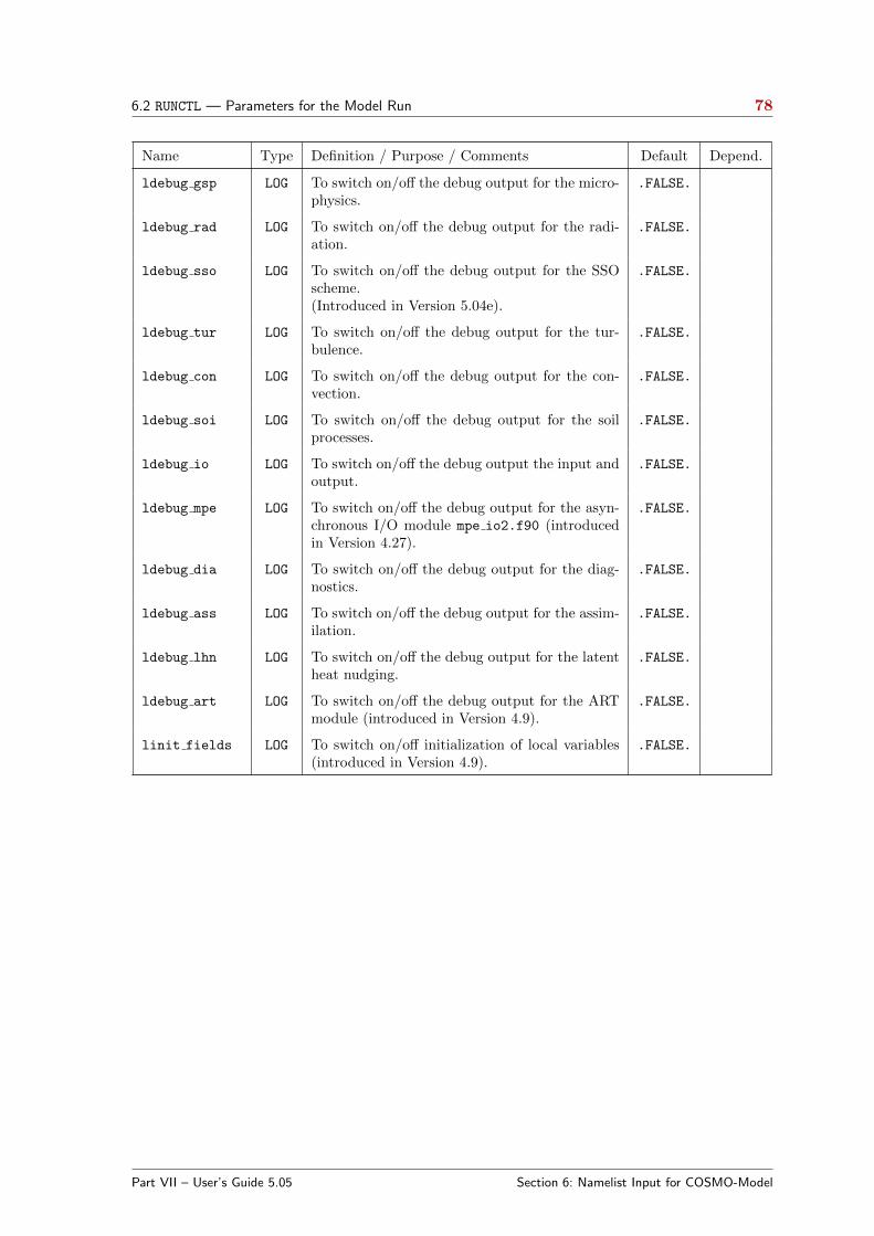
6.2 RUNCTL — Parameters for the Model Run 78
Name Type Definition / Purpose / Comments Default Depend.
ldebug gsp LOG To switch on/off the debug output for the micro-physics.
.FALSE.
ldebug rad LOG To switch on/off the debug output for the radi-ation.
.FALSE.
ldebug sso LOG To switch on/off the debug output for the SSOscheme.(Introduced in Version 5.04e).
.FALSE.
ldebug tur LOG To switch on/off the debug output for the tur-bulence.
.FALSE.
ldebug con LOG To switch on/off the debug output for the con-vection.
.FALSE.
ldebug soi LOG To switch on/off the debug output for the soilprocesses.
.FALSE.
ldebug io LOG To switch on/off the debug output the input andoutput.
.FALSE.
ldebug mpe LOG To switch on/off the debug output for the asyn-chronous I/O module mpe io2.f90 (introducedin Version 4.27).
.FALSE.
ldebug dia LOG To switch on/off the debug output for the diag-nostics.
.FALSE.
ldebug ass LOG To switch on/off the debug output for the assim-ilation.
.FALSE.
ldebug lhn LOG To switch on/off the debug output for the latentheat nudging.
.FALSE.
ldebug art LOG To switch on/off the debug output for the ARTmodule (introduced in Version 4.9).
.FALSE.
linit fields LOG To switch on/off initialization of local variables(introduced in Version 4.9).
.FALSE.
Part VII – User’s Guide 5.05 Section 6: Namelist Input for COSMO-Model
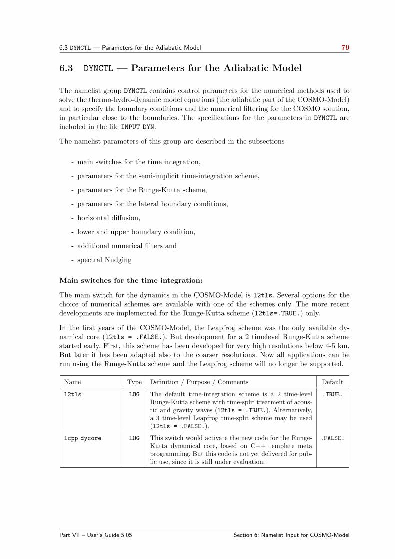
6.3 DYNCTL — Parameters for the Adiabatic Model 79
6.3 DYNCTL — Parameters for the Adiabatic Model
The namelist group DYNCTL contains control parameters for the numerical methods used tosolve the thermo-hydro-dynamic model equations (the adiabatic part of the COSMO-Model)and to specify the boundary conditions and the numerical filtering for the COSMO solution,in particular close to the boundaries. The specifications for the parameters in DYNCTL areincluded in the file INPUT DYN.
The namelist parameters of this group are described in the subsections
- main switches for the time integration,
- parameters for the semi-implicit time-integration scheme,
- parameters for the Runge-Kutta scheme,
- parameters for the lateral boundary conditions,
- horizontal diffusion,
- lower and upper boundary condition,
- additional numerical filters and
- spectral Nudging
Main switches for the time integration:
The main switch for the dynamics in the COSMO-Model is l2tls. Several options for thechoice of numerical schemes are available with one of the schemes only. The more recentdevelopments are implemented for the Runge-Kutta scheme (l2tls=.TRUE.) only.
In the first years of the COSMO-Model, the Leapfrog scheme was the only available dy-namical core (l2tls = .FALSE.). But development for a 2 timelevel Runge-Kutta schemestarted early. First, this scheme has been developed for very high resolutions below 4-5 km.But later it has been adapted also to the coarser resolutions. Now all applications can berun using the Runge-Kutta scheme and the Leapfrog scheme will no longer be supported.
Name Type Definition / Purpose / Comments Default
l2tls LOG The default time-integration scheme is a 2 time-levelRunge-Kutta scheme with time-split treatment of acous-tic and gravity waves (l2tls = .TRUE.). Alternatively,a 3 time-level Leapfrog time-split scheme may be used(l2tls = .FALSE.).
.TRUE.
lcpp dycore LOG This switch would activate the new code for the Runge-Kutta dynamical core, based on C++ template metaprogramming. But this code is not yet delivered for pub-lic use, since it is still under evaluation.
.FALSE.
Part VII – User’s Guide 5.05 Section 6: Namelist Input for COSMO-Model

6.3 DYNCTL — Parameters for the Adiabatic Model 80
Name Type Definition / Purpose / Comments Default
l euler dynamics LOG This variable allows to switch off/on the Euler dynami-cal core, i.e. advection, pressure gradient, divergence andbuoyancy-terms for the u,v,w,T and p-equation. It doesnot affect tracers or the Coriolis force, i.e. even if it isset to .FALSE., tracer advection and diffusion can takeplace and (if lcori=.TRUE.) Coriolis force can act.However, for the Leapfrog or semi-implicit dynamicalcore, the vertical advection of the dynamical variablesis still active, even if l euler dynamics=.FALSE..
.TRUE.
lsemi imp LOG Instead of the standard Leapfrog time-split scheme, aLeapfrog scheme with semi-implicit treatment of acous-tic and gravity waves may be used. This option worksonly with (l2tls = .FALSE.).Caution: the semi-implicit scheme is not yet fully evalu-ated.
.FALSE.
lcond LOG To include (.TRUE.) or exclude (.FALSE.) cloud watercondensation and evaporation during the forecast.
.TRUE.
lcori LOG Run with Coriolis force(has been moved from group /RUNCTL/ to here in Version4.8.
.TRUE.
lmetr LOG Run with metric terms.If .FALSE., the spherical geometry of the grid is ne-glected and the Coriolis force is assumed to be constanton the model domain (f-plane approximation).(has been moved from group /RUNCTL/ to here in Version4.8.
.TRUE.
lcori deep LOG To take coriolis terms (cos(ϕ)) into account. .FALSE.
ladv deep LOG To use all metric advective terms. .FALSE.
l satad dyn iter LOG If set to .FALSE., this disables the dynamical numberof iterations for the saturation adjustment in the rungekutta dynamical core and a fixed number of 3 iterationsis done then.(Introduced in Version 5.04a).
.TRUE.
Parameters for the semi-implicit time-integration scheme:
Name Type Definition / Purpose / Comments Default
ikrylow si INT Dimension of Krylow space for elliptic solver (GMRES). 20
iprint si INT Selects output of print statistics of the elliptical solver.> 1: Print statistics in file YUSOLVER.= 0: No statistics are printed.< 0: Print statistics on the screen.
0
maxit si INT Maximum number of iterations for elliptic solver. 200
eps si REAL Precision limit for the convergence of the solution from theelliptic solver.
10−8
Part VII – User’s Guide 5.05 Section 6: Namelist Input for COSMO-Model
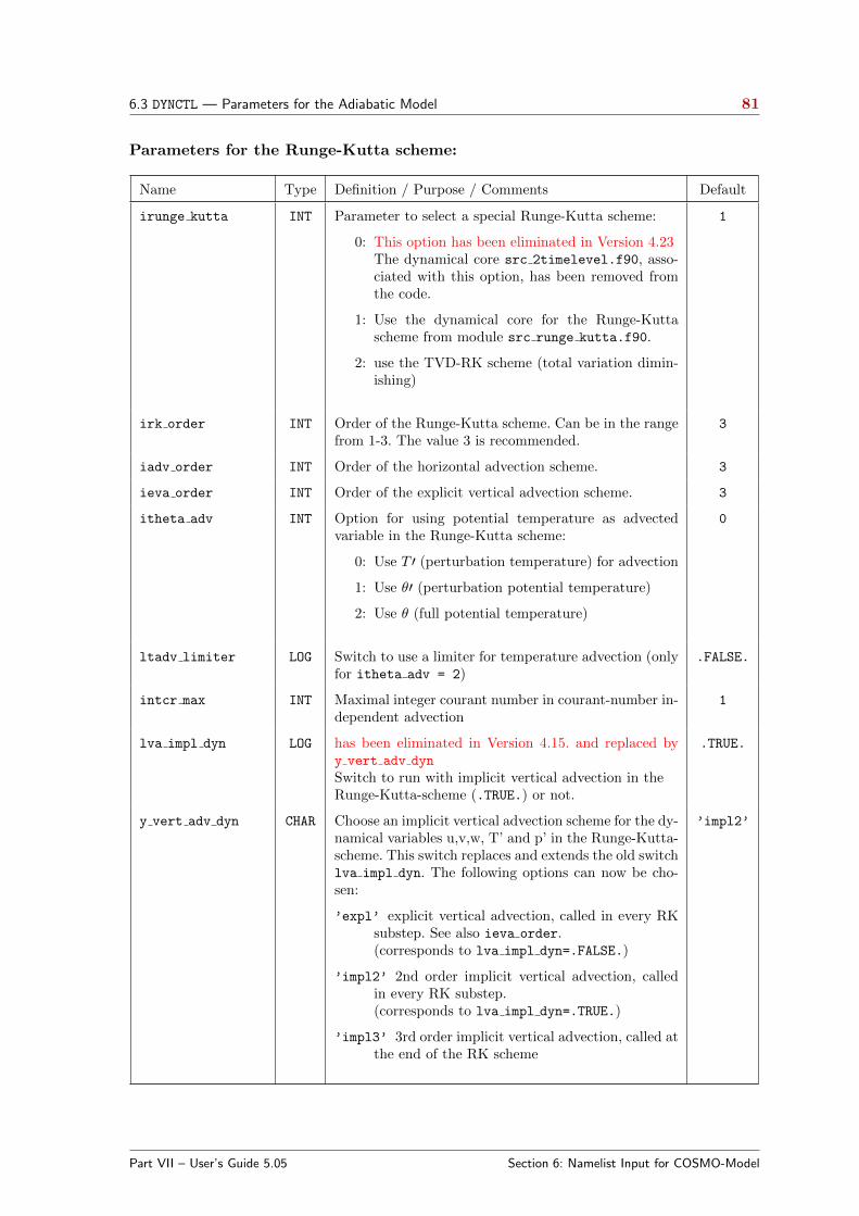
6.3 DYNCTL — Parameters for the Adiabatic Model 81
Parameters for the Runge-Kutta scheme:
Name Type Definition / Purpose / Comments Default
irunge kutta INT Parameter to select a special Runge-Kutta scheme:
0: This option has been eliminated in Version 4.23The dynamical core src 2timelevel.f90, asso-ciated with this option, has been removed fromthe code.
1: Use the dynamical core for the Runge-Kuttascheme from module src runge kutta.f90.
2: use the TVD-RK scheme (total variation dimin-ishing)
1
irk order INT Order of the Runge-Kutta scheme. Can be in the rangefrom 1-3. The value 3 is recommended.
3
iadv order INT Order of the horizontal advection scheme. 3
ieva order INT Order of the explicit vertical advection scheme. 3
itheta adv INT Option for using potential temperature as advectedvariable in the Runge-Kutta scheme:
0: Use T ′ (perturbation temperature) for advection
1: Use θ′ (perturbation potential temperature)
2: Use θ (full potential temperature)
0
ltadv limiter LOG Switch to use a limiter for temperature advection (onlyfor itheta adv = 2)
.FALSE.
intcr max INT Maximal integer courant number in courant-number in-dependent advection
1
lva impl dyn LOG has been eliminated in Version 4.15. and replaced byy vert adv dyn
Switch to run with implicit vertical advection in theRunge-Kutta-scheme (.TRUE.) or not.
.TRUE.
y vert adv dyn CHAR Choose an implicit vertical advection scheme for the dy-namical variables u,v,w, T’ and p’ in the Runge-Kutta-scheme. This switch replaces and extends the old switchlva impl dyn. The following options can now be cho-sen:
’expl’ explicit vertical advection, called in every RKsubstep. See also ieva order.(corresponds to lva impl dyn=.FALSE.)
’impl2’ 2nd order implicit vertical advection, calledin every RK substep.(corresponds to lva impl dyn=.TRUE.)
’impl3’ 3rd order implicit vertical advection, called atthe end of the RK scheme
’impl2’
Part VII – User’s Guide 5.05 Section 6: Namelist Input for COSMO-Model

6.3 DYNCTL — Parameters for the Adiabatic Model 82
Name Type Definition / Purpose / Comments Default
itype fast waves INT Parameter to select the treatment of fast waves:
1: Old scheme (from module fast waves rk.f90).
2: New scheme (from module fast waves sc.f90)with
– proper weightings for all vertical discretiza-tions,
– divergence operator in strong conservationform,
– (optionally) isotropic (fully 3D) divergencedamping,
– (optionally) Mahrer (1984) discretization.
This is the new default (from Version 4.27 on).
2
lhor pgrad Mahrer LOG (Only for itype fast waves=2)The horizontal pressure gradient (i.e. in the u- and v-equations) is either calculated in the terrain-followingsystem (.FALSE.) or by interpolation of p′ to a hori-zontal plane (Mahrer (1984) MWR) (.TRUE.). (See alsoBaldauf (2013))
.FALSE.
divdamp slope REAL (Only for itype fast waves=2)Exceed the theoretical slope stability criterion of thedivergence damping.After a bug fix in Version 5.04a the range and the de-fault value have changed: Possible range now is between0.1 and 3.0. New Default is 1.0
20.0
1.0
l 3D div damping LOG (Only for itype fast waves=2)The artificial divergence damping either acts only onthe u- and v-equation (.FALSE.) or in a fully isotropic3D manner (.TRUE.). The latter version is more timeconsuming (and less tested until now). (See also Baldauf(2013) and Baldauf (2014))
.FALSE.
Part VII – User’s Guide 5.05 Section 6: Namelist Input for COSMO-Model
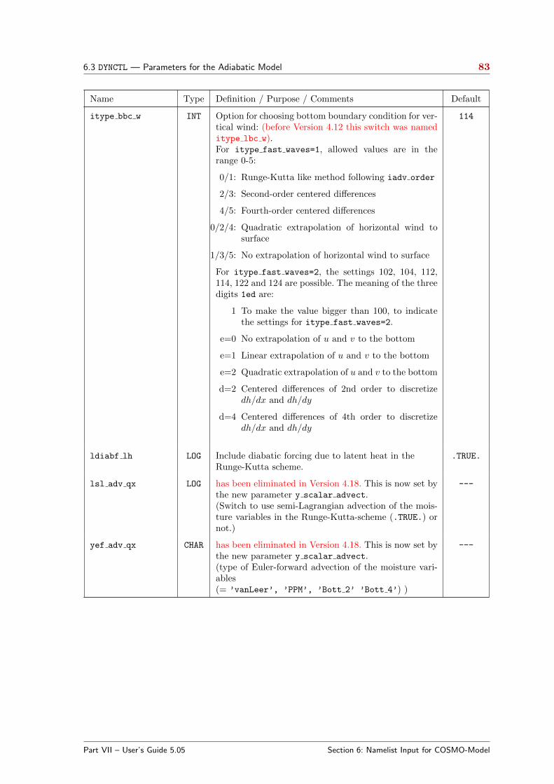
6.3 DYNCTL — Parameters for the Adiabatic Model 83
Name Type Definition / Purpose / Comments Default
itype bbc w INT Option for choosing bottom boundary condition for ver-tical wind: (before Version 4.12 this switch was nameditype lbc w).For itype fast waves=1, allowed values are in therange 0-5:
0/1: Runge-Kutta like method following iadv order
2/3: Second-order centered differences
4/5: Fourth-order centered differences
0/2/4: Quadratic extrapolation of horizontal wind tosurface
1/3/5: No extrapolation of horizontal wind to surface
For itype fast waves=2, the settings 102, 104, 112,114, 122 and 124 are possible. The meaning of the threedigits 1ed are:
1 To make the value bigger than 100, to indicatethe settings for itype fast waves=2.
e=0 No extrapolation of u and v to the bottom
e=1 Linear extrapolation of u and v to the bottom
e=2 Quadratic extrapolation of u and v to the bottom
d=2 Centered differences of 2nd order to discretizedh/dx and dh/dy
d=4 Centered differences of 4th order to discretizedh/dx and dh/dy
114
ldiabf lh LOG Include diabatic forcing due to latent heat in theRunge-Kutta scheme.
.TRUE.
lsl adv qx LOG has been eliminated in Version 4.18. This is now set bythe new parameter y scalar advect.(Switch to use semi-Lagrangian advection of the mois-ture variables in the Runge-Kutta-scheme (.TRUE.) ornot.)
---
yef adv qx CHAR has been eliminated in Version 4.18. This is now set bythe new parameter y scalar advect.(type of Euler-forward advection of the moisture vari-ables(= ’vanLeer’, ’PPM’, ’Bott 2’ ’Bott 4’) )
---
Part VII – User’s Guide 5.05 Section 6: Namelist Input for COSMO-Model
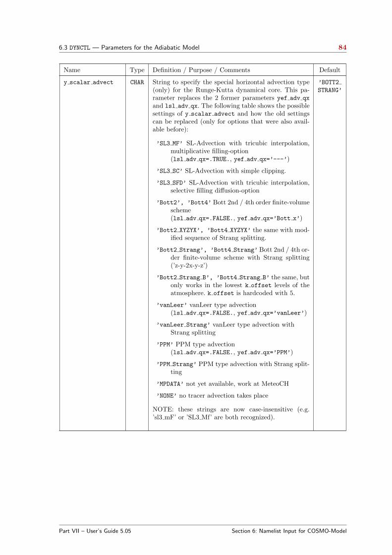
6.3 DYNCTL — Parameters for the Adiabatic Model 84
Name Type Definition / Purpose / Comments Default
y scalar advect CHAR String to specify the special horizontal advection type(only) for the Runge-Kutta dynamical core. This pa-rameter replaces the 2 former parameters yef adv qx
and lsl adv qx. The following table shows the possiblesettings of y scalar advect and how the old settingscan be replaced (only for options that were also avail-able before):
’SL3 MF’ SL-Advection with tricubic interpolation,multiplicative filling-option(lsl adv qx=.TRUE., yef adv qx=’---’)
’SL3 SC’ SL-Advection with simple clipping.
’SL3 SFD’ SL-Advection with tricubic interpolation,selective filling diffusion-option
’Bott2’, ’Bott4’ Bott 2nd / 4th order finite-volumescheme(lsl adv qx=.FALSE., yef adv qx=’Bott x’)
’Bott2 XYZYX’, ’Bott4 XYZYX’ the same with mod-ified sequence of Strang splitting.
’Bott2 Strang’, ’Bott4 Strang’ Bott 2nd / 4th or-der finite-volume scheme with Strang splitting(’z-y-2x-y-z’)
’Bott2 Strang B’, ’Bott4 Strang B’ the same, butonly works in the lowest k offset levels of theatmosphere. k offset is hardcoded with 5.
’vanLeer’ vanLeer type advection(lsl adv qx=.FALSE., yef adv qx=’vanLeer’)
’vanLeer Strang’ vanLeer type advection withStrang splitting
’PPM’ PPM type advection(lsl adv qx=.FALSE., yef adv qx=’PPM’)
’PPM Strang’ PPM type advection with Strang split-ting
’MPDATA’ not yet available, work at MeteoCH
’NONE’ no tracer advection takes place
NOTE: these strings are now case-insensitive (e.g.’sl3 mF’ or ’SL3 Mf’ are both recognized).
’BOTT2
STRANG’
Part VII – User’s Guide 5.05 Section 6: Namelist Input for COSMO-Model

6.3 DYNCTL — Parameters for the Adiabatic Model 85
Parameters for the lateral boundary conditions:
Name Type Definition / Purpose / Comments Default
lw freeslip LOG Free-slip lateral boundary conditions are used for w
by default in case of non-periodic Davies-type lateralboundaries. Otherwise, w must be specified along theboundaries.It is recommended to use free-slip lateral boundaryconditions for real-data simulations.
.TRUE.
lexpl lbc LOG eliminated in 5.1!: Now only the explicit formulationof the lateral boundary relaxation is possible.Chooses an explicit formulation of the lateral bound-ary relaxation.
.TRUE.
crltau REAL has been renamed in 5.1 to crltau inv!To set the time factor for the explicit formulation oflateral boundary relaxation: τr = crltau ·∆t.
1.0
crltau inv REAL NOTE: Former name was crltau and the meaningreally is crltau inv = 1/crltau.Factor for relaxation time: 1/τr = crltau inv ·1/dt.The advantage of this replacement lies in the fact,that crltau inv=0 completely switches off the re-laxation (this was not possible before).
1.0
rlwidth REAL If lexpl lbc = .TRUE., this parameter specifies thewidth of the relaxation layer in meters. It shouldbe 10 to 15 times the grid mesh size in meters, butshould not exceed 0.25 times the full domain size.
85000.0
itype outflow qrsg INT To choose the type of relaxation treatment for qr,
qs, qg. (before Version 4.9 this switch was nameditype lbcqx).
1: qr, qs, qg are treated with the same lateralboundary relaxation as the other variables
2: no relaxation of qr, qs, qg is done at outflowboundary points
1
itype lbc qrsg INT To choose the type of lateral boundary treatmentfor qr, qs, qg, i.e., which values are used at theboundary zone.
1: A zero-gradient condition is used for qr, qs,
qg
2: qr, qs, qg are set to 0.0 at the boundaryzone
3: No presetting is done in the whole the bound-ary zone (must not be chosen for Leapfrog ap-plications).
1
lradlbc LOG To run with radiative lateral boundary conditions (if.TRUE.), or with Davies conditions (if .FALSE.).(In Version 4.5 this switch has been moved from thegroup RUNCTL to DYNCTL).
.FALSE.
Part VII – User’s Guide 5.05 Section 6: Namelist Input for COSMO-Model
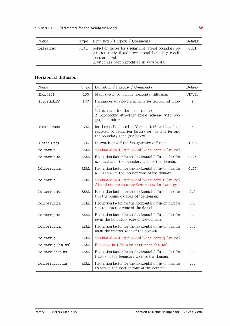
6.3 DYNCTL — Parameters for the Adiabatic Model 86
Name Type Definition / Purpose / Comments Default
relax fac REAL reduction factor for strength of lateral boundary re-laxation (only if radiative lateral boundary condi-tions are used).(Switch has been introduced in Version 4.5).
0.01
Horizontal diffusion:
Name Type Definition / Purpose / Comments Default
lhordiff LOG Main switch to include horizontal diffusion. .TRUE.
itype hdiff INT Parameter to select a scheme for horizontal diffu-sion.1: Regular 4th-order linear scheme2: Monotonic 4th-order linear scheme with oro-graphic limiter
2
lhdiff mask LOG has been eliminated in Version 4.12 and has beenreplaced by reduction factors for the interior andthe boundary zone (see below).
-
l diff Smag LOG to switch on/off the Smagorinsky diffusion. .TRUE.
hd corr u REAL eliminated in 4.12; replaced by hd corr u [in,bd]
hd corr u bd REAL Reduction factor for the horizontal diffusion flux foru, v and w in the boundary zone of the domain.
0.25
hd corr u in REAL Reduction factor for the horizontal diffusion flux foru, v and w in the interior zone of the domain.
0.25
hd corr t REAL eliminated in 4.12; replaced by hd corr t [in,bd]
Also, there are separate factors now for t and pp.
hd corr t bd REAL Reduction factor for the horizontal diffusion flux fort in the boundary zone of the domain.
0.0
hd corr t in REAL Reduction factor for the horizontal diffusion flux fort in the interior zone of the domain.
0.0
hd corr p bd REAL Reduction factor for the horizontal diffusion flux forpp in the boundary zone of the domain.
0.0
hd corr p in REAL Reduction factor for the horizontal diffusion flux forpp in the interior zone of the domain.
0.0
hd corr q REAL eliminated in 4.12; replaced by hd corr q [in,bd]
hd corr q [in,bd] REAL Renamed in 4.26 to hd corr trcr [in,bd]
hd corr trcr bd REAL Reduction factor for the horizontal diffusion flux fortracers in the boundary zone of the domain.
0.0
hd corr trcr in REAL Reduction factor for the horizontal diffusion flux fortracers in the interior zone of the domain.
0.0
Part VII – User’s Guide 5.05 Section 6: Namelist Input for COSMO-Model

6.3 DYNCTL — Parameters for the Adiabatic Model 87
Name Type Definition / Purpose / Comments Default
hd dhmax REAL Threshold value for the maximum height difference(m) between adjacent gridpoints in the orographicflux limiter. With increasing height difference, thediffusive fluxes are gradually decreased to becomezero at hd dhmax. Active only for itype hdiff =
2.Caution: The parameter hd dhmax should be ad-justed when changing the grid spacing.
250.0
l diff cold pools LOG Use targeted diffusion for cold pools. It should avoidunrealistic undershootings in the temperature fieldnear the bottom, if the value of a grid point is morethan thresh cold pool degrees Kelvin less thanthe average value of the surrounding.
.TRUE.
l diff cold pools uv LOG Use a different method for targeted diffusion forcold pools. For this scheme the threshold is com-puted over the 8 neighboring grid points insteadof only 4 to detect a cold pool and a box-filter isapplied on the detected thresholds. This increasesthe application domain for a detected cold poolfrom 1 to 9 grid points.To activate this new method, alsol diff cold pools has to be set to .TRUE.
.FALSE.
thresh cold pool REAL Threshold for targeted diffusion for cold pools. Rea-sonable values are thresh cold pool ∈ [5.0, 20.0].
10.0
Lower and upper boundary condition:
Name Type Definition / Purpose / Comments Default
lspubc LOG Option to use a sponge layer with Rayleigh damping in theupper levels of the model domain. If lspubc =.FALSE., a rigidlid upper boundary condition is used.
.TRUE.
itype spubc INT To choose the type of Rayleigh damping in the upper levels.
1: chooses the damping against boundary fields;
2: chooses the damping against filtered forecast fields (canbe chosen, if the boundary data is only available onframes.
3: New sponge layer near upper model boundary (accord-ing to Klemp et al.)
1
nfi spubc2 INT Number of applications of smoother for the determinationof the large scale field used in the Rayleigh damping withitype spubc=2
10
lrubc LOG Option to use a radiative upper boundary condition.Not yet implemented.
.FALSE.
Part VII – User’s Guide 5.05 Section 6: Namelist Input for COSMO-Model
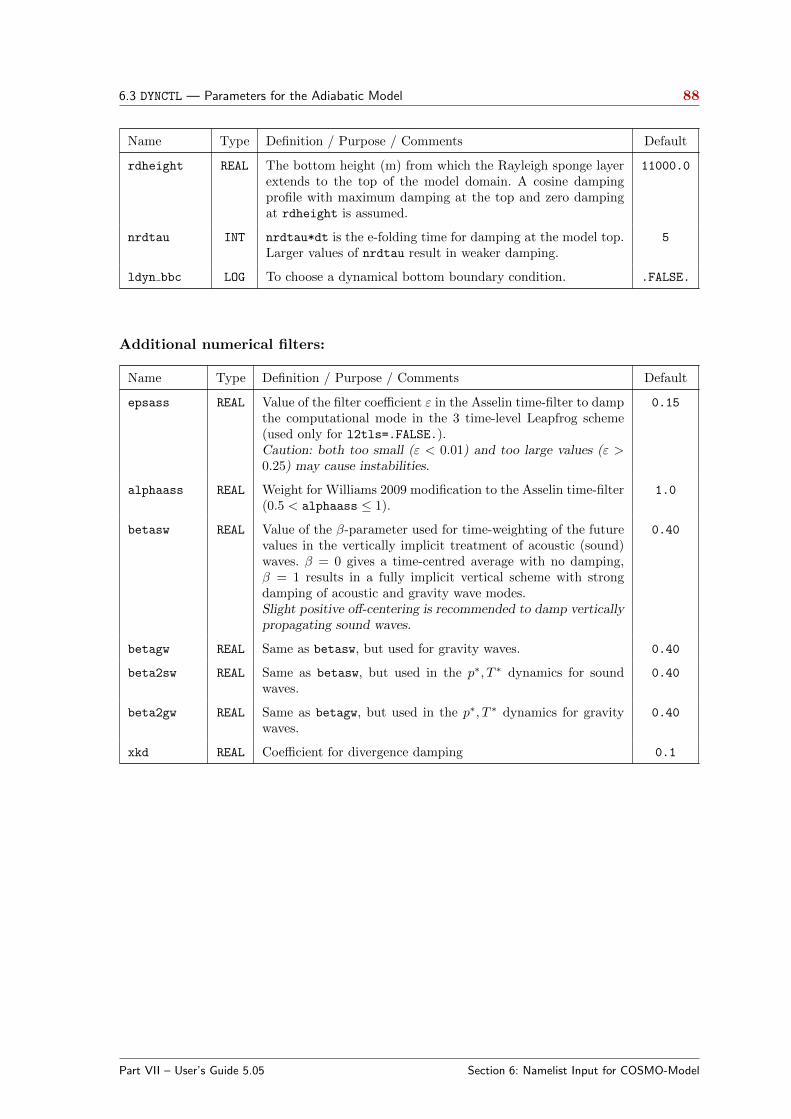
6.3 DYNCTL — Parameters for the Adiabatic Model 88
Name Type Definition / Purpose / Comments Default
rdheight REAL The bottom height (m) from which the Rayleigh sponge layerextends to the top of the model domain. A cosine dampingprofile with maximum damping at the top and zero dampingat rdheight is assumed.
11000.0
nrdtau INT nrdtau*dt is the e-folding time for damping at the model top.Larger values of nrdtau result in weaker damping.
5
ldyn bbc LOG To choose a dynamical bottom boundary condition. .FALSE.
Additional numerical filters:
Name Type Definition / Purpose / Comments Default
epsass REAL Value of the filter coefficient ε in the Asselin time-filter to dampthe computational mode in the 3 time-level Leapfrog scheme(used only for l2tls=.FALSE.).Caution: both too small (ε < 0.01) and too large values (ε >0.25) may cause instabilities.
0.15
alphaass REAL Weight for Williams 2009 modification to the Asselin time-filter(0.5 < alphaass ≤ 1).
1.0
betasw REAL Value of the β-parameter used for time-weighting of the futurevalues in the vertically implicit treatment of acoustic (sound)waves. β = 0 gives a time-centred average with no damping,β = 1 results in a fully implicit vertical scheme with strongdamping of acoustic and gravity wave modes.Slight positive off-centering is recommended to damp verticallypropagating sound waves.
0.40
betagw REAL Same as betasw, but used for gravity waves. 0.40
beta2sw REAL Same as betasw, but used in the p∗, T ∗ dynamics for soundwaves.
0.40
beta2gw REAL Same as betagw, but used in the p∗, T ∗ dynamics for gravitywaves.
0.40
xkd REAL Coefficient for divergence damping 0.1
Part VII – User’s Guide 5.05 Section 6: Namelist Input for COSMO-Model
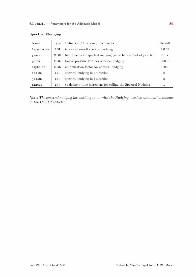
6.3 DYNCTL — Parameters for the Adiabatic Model 89
Spectral Nudging
Name Type Definition / Purpose / Comments Default
lspecnudge LOG to switch on/off spectral nudging .FALSE.
yvarsn CHAR list of fields for spectral nudging (must be a subset of yvarbd U, V
pp sn REAL lowest pressure level for spectral nudging 850.0
alpha sn REAL amplification factor for spectral nudging 0.05
isc sn INT spectral nudging in i-direction 2
jsc sn INT spectral nudging in j-direction 2
nincsn INT to define a time increment for calling the Spectral Nudging 1
Note: The spectral nudging has nothing to do with the Nudging, used as assimilation schemein the COSMO-Model.
Part VII – User’s Guide 5.05 Section 6: Namelist Input for COSMO-Model
6.4 PHYCTL — Parameters for the Diabatic Model 90
6.4 PHYCTL — Parameters for the Diabatic Model
The namelist group PHYCTL contains parameters controlling the physical parameterizations.All parameters are only active if the parameter lphys in Namelist /RUNCTL/ is set to .TRUE.
in order to enable physical parameterizations. There is one main switch for each physicalprocess to turn on/off this process and to activate additional parameters and sub-options forthe corresponding parameterisation. The specifications for the parameters in /PHYCTL/ areincluded in the file INPUT PHY.
The namelist parameters of this group are described in the subsections
- Grid-Scale Precipitation,
- Radiation,
- Moist Convection,
- Vertical turbulent diffusion,
- Surface layer fluxes,
- Soil Processes
- Subgrid Scale Orography
The switch to activate single column model runs is necessary in several schemes, therefore itis not assigned to a special group:
Name Type Definition / Purpose / Comments Default
lscm LOG Main switch to run the single column model.Note, that up to the single column model is not fully imple-mented in the COSMO-Model.
.FALSE.
Part VII – User’s Guide 5.05 Section 6: Namelist Input for COSMO-Model
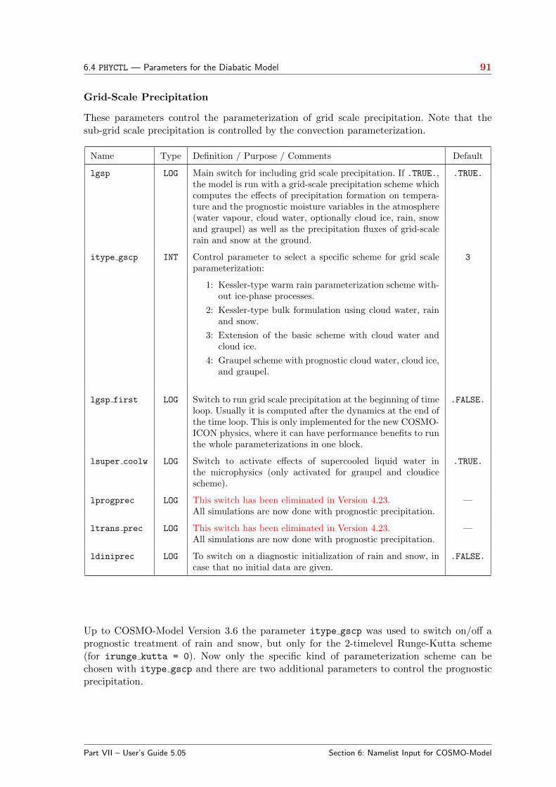
6.4 PHYCTL — Parameters for the Diabatic Model 91
Grid-Scale Precipitation
These parameters control the parameterization of grid scale precipitation. Note that thesub-grid scale precipitation is controlled by the convection parameterization.
Name Type Definition / Purpose / Comments Default
lgsp LOG Main switch for including grid scale precipitation. If .TRUE.,the model is run with a grid-scale precipitation scheme whichcomputes the effects of precipitation formation on tempera-ture and the prognostic moisture variables in the atmosphere(water vapour, cloud water, optionally cloud ice, rain, snowand graupel) as well as the precipitation fluxes of grid-scalerain and snow at the ground.
.TRUE.
itype gscp INT Control parameter to select a specific scheme for grid scaleparameterization:
1: Kessler-type warm rain parameterization scheme with-out ice-phase processes.
2: Kessler-type bulk formulation using cloud water, rainand snow.
3: Extension of the basic scheme with cloud water andcloud ice.
4: Graupel scheme with prognostic cloud water, cloud ice,and graupel.
3
lgsp first LOG Switch to run grid scale precipitation at the beginning of timeloop. Usually it is computed after the dynamics at the end ofthe time loop. This is only implemented for the new COSMO-ICON physics, where it can have performance benefits to runthe whole parameterizations in one block.
.FALSE.
lsuper coolw LOG Switch to activate effects of supercooled liquid water inthe microphysics (only activated for graupel and cloudicescheme).
.TRUE.
lprogprec LOG This switch has been eliminated in Version 4.23.All simulations are now done with prognostic precipitation.
—
ltrans prec LOG This switch has been eliminated in Version 4.23.All simulations are now done with prognostic precipitation.
—
ldiniprec LOG To switch on a diagnostic initialization of rain and snow, incase that no initial data are given.
.FALSE.
Up to COSMO-Model Version 3.6 the parameter itype gscp was used to switch on/off aprognostic treatment of rain and snow, but only for the 2-timelevel Runge-Kutta scheme(for irunge kutta = 0). Now only the specific kind of parameterization scheme can bechosen with itype gscp and there are two additional parameters to control the prognosticprecipitation.
Part VII – User’s Guide 5.05 Section 6: Namelist Input for COSMO-Model

6.4 PHYCTL — Parameters for the Diabatic Model 92
Radiation
The following parameters control the Ritter-Geleyn radiation parameterization scheme of theCOSMO-Model. Here, among others, the frequency of the calculation, the surface albedo,the background aerosols and the greenhouse gas concentration scenario can be specified.
Name Type Definition / Purpose / Comments Default Depend.
lrad LOG Main switch for including radiation. If .TRUE.,the model is run with the radiation scheme whichcomputes heating rates in the atmosphere (solarand thermal) and the energy balance (solar andthermal) at the ground. To save computing time,the radiation scheme will be called at certain timeintervalls defined by nincrad or hincrad. Be-tween two consecutive calls of the scheme, theradiative heating rates are kept constant.
.TRUE.
nincrad INT Interval (in time steps) between two calls of theradiation scheme.
360 P,dt
hincrad REAL As nincrad, but time interval in hours. In gen-eral, an interval of 0.5 – 1 hour yields sufficientaccuracy.Can be specified alternatively to nincrad.
0.0 P,dt
icldm rad INT Parameter to select the mode of cloud represen-tation (i.e. cloud cover, and cloud water and icecontent) as input to the radiation parameteriza-tion.
0: No clouds are considered.
1: Only grid-scale clouds are considered.
2: Grid- and sub-grid scale water clouds areconsidered; cloud cover and water con-tent are calculated according to a relative-humidity criterion (itype wcld = 1) or astatistical closure (itype wcld = 2).
3: Grid- and sub-grid scale (including convec-tive) water and ice clouds are considered;cloud cover, water content and ice contentare calculated according to the diagnosisbased on a relative humidity scheme. (Butnote that also cloud ice is considered here!)
4: (at the moment) same as 3.
4
lforest LOG Switch to choose the external parameter fieldsmodifying the snow albedo of evergreen and de-ciduous forest. (itype alb has to be chosen accord-ingly) Recommended: .TRUE.
.FALSE. R
nradcoarse INT If nradcoarse > 1, the radiation is computedon a coarser grid to save computation time.nradcoarse grid points in every horizontal di-mension are combined. Maximal possible value isnboundlines.
1 P
Part VII – User’s Guide 5.05 Section 6: Namelist Input for COSMO-Model
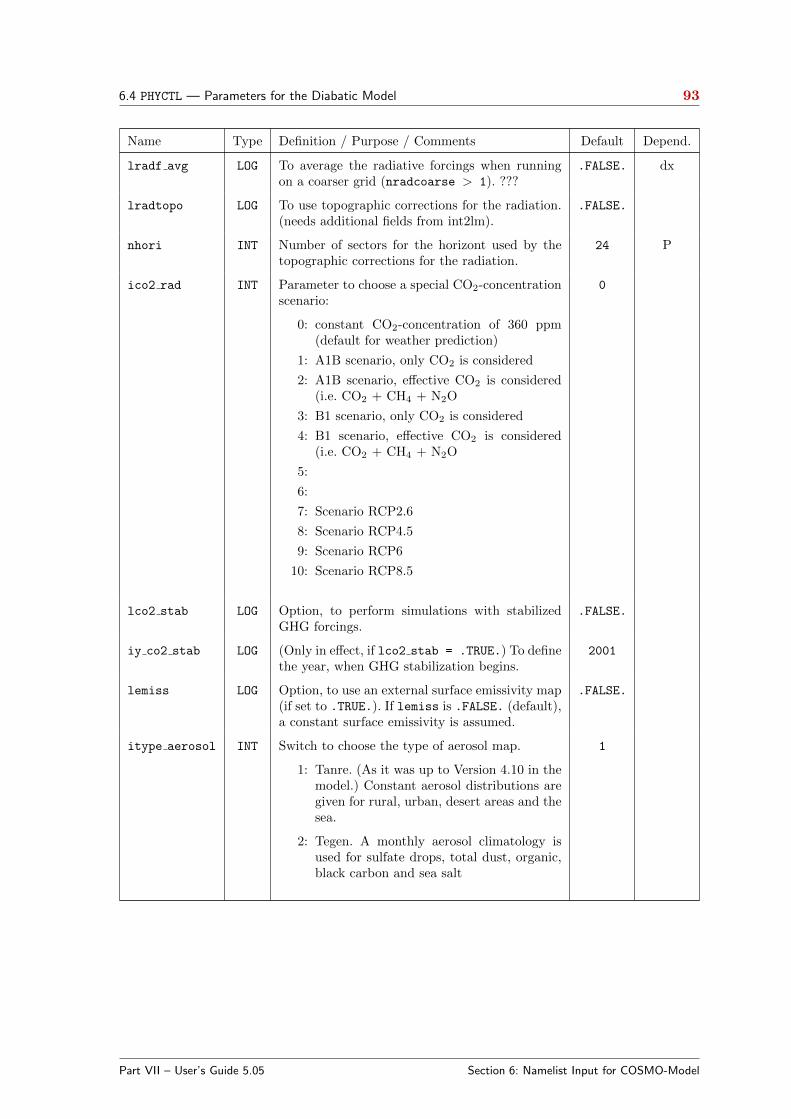
6.4 PHYCTL — Parameters for the Diabatic Model 93
Name Type Definition / Purpose / Comments Default Depend.
lradf avg LOG To average the radiative forcings when runningon a coarser grid (nradcoarse > 1). ???
.FALSE. dx
lradtopo LOG To use topographic corrections for the radiation.(needs additional fields from int2lm).
.FALSE.
nhori INT Number of sectors for the horizont used by thetopographic corrections for the radiation.
24 P
ico2 rad INT Parameter to choose a special CO2-concentrationscenario:
0: constant CO2-concentration of 360 ppm(default for weather prediction)
1: A1B scenario, only CO2 is considered
2: A1B scenario, effective CO2 is considered(i.e. CO2 + CH4 + N2O
3: B1 scenario, only CO2 is considered
4: B1 scenario, effective CO2 is considered(i.e. CO2 + CH4 + N2O
5:
6:
7: Scenario RCP2.6
8: Scenario RCP4.5
9: Scenario RCP6
10: Scenario RCP8.5
0
lco2 stab LOG Option, to perform simulations with stabilizedGHG forcings.
.FALSE.
iy co2 stab LOG (Only in effect, if lco2 stab = .TRUE.) To definethe year, when GHG stabilization begins.
2001
lemiss LOG Option, to use an external surface emissivity map(if set to .TRUE.). If lemiss is .FALSE. (default),a constant surface emissivity is assumed.
.FALSE.
itype aerosol INT Switch to choose the type of aerosol map.
1: Tanre. (As it was up to Version 4.10 in themodel.) Constant aerosol distributions aregiven for rural, urban, desert areas and thesea.
2: Tegen. A monthly aerosol climatology isused for sulfate drops, total dust, organic,black carbon and sea salt
1
Part VII – User’s Guide 5.05 Section 6: Namelist Input for COSMO-Model

6.4 PHYCTL — Parameters for the Diabatic Model 94
Name Type Definition / Purpose / Comments Default Depend.
itype albedo INT Switch to choose the type of solar surface albedo.This parameter has been introduced in Version4.23.
1: surface albedo is a function of soiltype(method up to now and still default)
2: surface albedo is determined as a weightedmean value of two external fields for dryand for saturated soil. As a weighting factorthe relative soil moisture saturation for thetop soil layer is used.
3: A background albedo is prescribed by ex-ternal fields, which give average values forevery month. The actual surface albedo isdetermined by a linear interpolation be-tween two monthly values, depending onthe day. This is done in INT2LM.
4: The vegetation albedo is modified by for-est fraction. Note, that for this type, alsolforest has to be set to .TRUE.
1
Part VII – User’s Guide 5.05 Section 6: Namelist Input for COSMO-Model

6.4 PHYCTL — Parameters for the Diabatic Model 95
Moist Convection
These parameters specify the convection parameterization used. In particular at resolutionsbelow 3 km the deep convection parameterization should be switched off, since this processis mainly a grid scale process for such high horizontal resolutions. It is possible to run withthe shallow convection scheme then.
the model is run with a moist convection parameterization,
If a subgrid-scale (deep) convection scheme is used (lconv=.TRUE.), it computes the effect ofmoist convection on temperature, water vapour and horizontal wind in the atmosphere, andthe precipitation rates of rain and snow at the ground. To save computing time, the convec-tion scheme may not be called every time step, but at certain intervals defined by nincconv.Between two consecutive calls of the scheme, the convective tendencies and precipitationfluxes are kept constant.
There are two different schemes for deep convection: Tiedtke and (since version 5.04b)Tiedtke-Bechtold (the IFS convection scheme). A former implementation of Kain-Fritschconvection scheme has never been finished and was eliminated some time ago.
Name Type Definition / Purpose / Comments Default
lconv LOG Main switch for including a subgrid-scale convection. .FALSE.
ltiedtke LOG Eliminated ; replaced by itype conv in Version 4.4
lkainfri LOG Eliminated ; replaced by itype conv in Version 4.4
lshallow LOG Eliminated ; replaced by itype conv in Version 4.4
itype conv INT To specify the type of convection parameterization
0: Tiedtke scheme
1: This option has been eliminated
2: Tiedtke-Bechtold scheme
3: Shallow convection based on Tiedtke scheme
0
nincconv INT Interval (in time steps) between two calls of the convectionscheme.
4
lconf avg LOG Switch to apply a horizontal smoothing of the convective forc-ings (moisture convergence, surface moisture flux and verticalvelocity) prior to calling the convection scheme.
.TRUE.
lcape LOG Enables a CAPE-type closure within the Tiedtke convectionscheme (not fully tested yet).
.FALSE.
lctke LOG Enables a turbulent kinetic energy closure within the Tiedtkescheme (not fully tested yet).
.FALSE.
lconv inst LOG Switch to write instantaneous (.TRUE.) or aggregate (.FALSE.)values of top con and bas con to model output.
.FALSE.
Part VII – User’s Guide 5.05 Section 6: Namelist Input for COSMO-Model
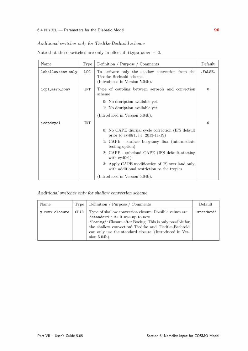
6.4 PHYCTL — Parameters for the Diabatic Model 96
Additional switches only for Tiedtke-Bechtold scheme
Note that these switches are only in effect if itype conv = 2.
Name Type Definition / Purpose / Comments Default
lshallowconv only LOG To activate only the shallow convection from theTiedtke-Bechtold scheme.(Introduced in Version 5.04h).
.FALSE.
icpl aero conv INT Type of coupling between aerosols and convectionscheme
0: No desription available yet.
1: No desription available yet.
(Introduced in Version 5.04b).
0
icapdcycl INT
0: No CAPE diurnal cycle correction (IFS defaultprior to cy40r1, i.e. 2013-11-19)
1: CAPE - surface buoyancy flux (intermediatetesting option)
2: CAPE - subcloud CAPE (IFS default startingwith cy40r1)
3: Apply CAPE modification of (2) over land only,with additional restriction to the tropics
(Introduced in Version 5.04b).
0
Additional switches only for shallow convection scheme
Name Type Definition / Purpose / Comments Default
y conv closure CHAR Type of shallow convection closure: Possible values are:’standard’: As it was up to now’Boeing’: Closure after Boeing. This is only possible forthe shallow convection! Tiedtke and Tiedtke-Bechtoldcan only use the standard closure. (Introduced in Ver-sion 5.04b).
’standard’
Part VII – User’s Guide 5.05 Section 6: Namelist Input for COSMO-Model
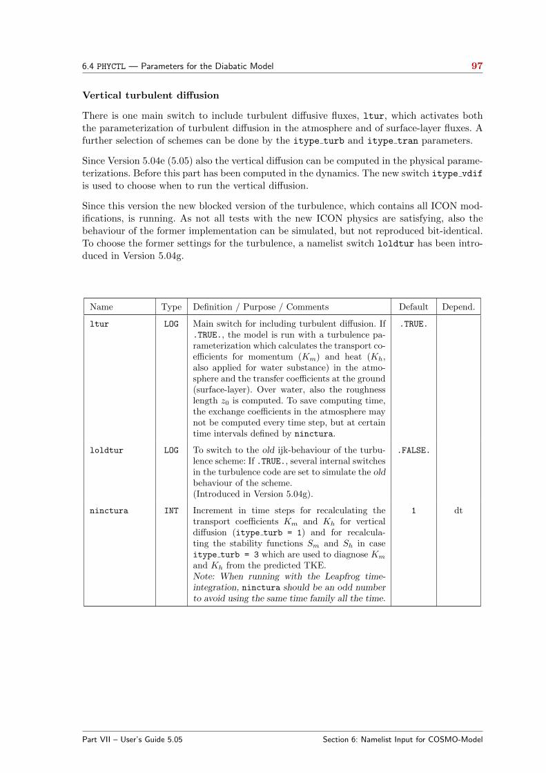
6.4 PHYCTL — Parameters for the Diabatic Model 97
Vertical turbulent diffusion
There is one main switch to include turbulent diffusive fluxes, ltur, which activates boththe parameterization of turbulent diffusion in the atmosphere and of surface-layer fluxes. Afurther selection of schemes can be done by the itype turb and itype tran parameters.
Since Version 5.04e (5.05) also the vertical diffusion can be computed in the physical parame-terizations. Before this part has been computed in the dynamics. The new switch itype vdif
is used to choose when to run the vertical diffusion.
Since this version the new blocked version of the turbulence, which contains all ICON mod-ifications, is running. As not all tests with the new ICON physics are satisfying, also thebehaviour of the former implementation can be simulated, but not reproduced bit-identical.To choose the former settings for the turbulence, a namelist switch loldtur has been intro-duced in Version 5.04g.
Name Type Definition / Purpose / Comments Default Depend.
ltur LOG Main switch for including turbulent diffusion. If.TRUE., the model is run with a turbulence pa-rameterization which calculates the transport co-efficients for momentum (Km) and heat (Kh,also applied for water substance) in the atmo-sphere and the transfer coefficients at the ground(surface-layer). Over water, also the roughnesslength z0 is computed. To save computing time,the exchange coefficients in the atmosphere maynot be computed every time step, but at certaintime intervals defined by ninctura.
.TRUE.
loldtur LOG To switch to the old ijk-behaviour of the turbu-lence scheme: If .TRUE., several internal switchesin the turbulence code are set to simulate the oldbehaviour of the scheme.(Introduced in Version 5.04g).
.FALSE.
ninctura INT Increment in time steps for recalculating thetransport coefficients Km and Kh for verticaldiffusion (itype turb = 1) and for recalcula-ting the stability functions Sm and Sh in caseitype turb = 3 which are used to diagnose Km
and Kh from the predicted TKE.Note: When running with the Leapfrog time-integration, ninctura should be an odd numberto avoid using the same time family all the time.
1 dt
Part VII – User’s Guide 5.05 Section 6: Namelist Input for COSMO-Model
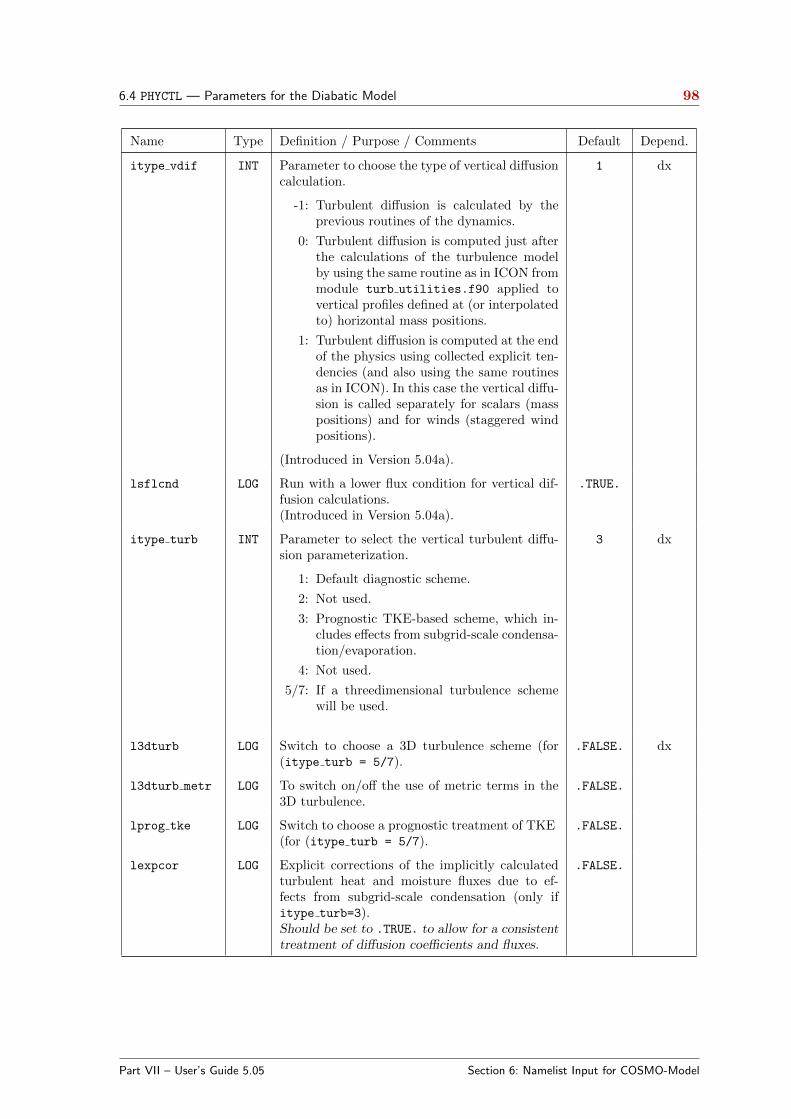
6.4 PHYCTL — Parameters for the Diabatic Model 98
Name Type Definition / Purpose / Comments Default Depend.
itype vdif INT Parameter to choose the type of vertical diffusioncalculation.
-1: Turbulent diffusion is calculated by theprevious routines of the dynamics.
0: Turbulent diffusion is computed just afterthe calculations of the turbulence modelby using the same routine as in ICON frommodule turb utilities.f90 applied tovertical profiles defined at (or interpolatedto) horizontal mass positions.
1: Turbulent diffusion is computed at the endof the physics using collected explicit ten-dencies (and also using the same routinesas in ICON). In this case the vertical diffu-sion is called separately for scalars (masspositions) and for winds (staggered windpositions).
(Introduced in Version 5.04a).
1 dx
lsflcnd LOG Run with a lower flux condition for vertical dif-fusion calculations.(Introduced in Version 5.04a).
.TRUE.
itype turb INT Parameter to select the vertical turbulent diffu-sion parameterization.
1: Default diagnostic scheme.
2: Not used.
3: Prognostic TKE-based scheme, which in-cludes effects from subgrid-scale condensa-tion/evaporation.
4: Not used.
5/7: If a threedimensional turbulence schemewill be used.
3 dx
l3dturb LOG Switch to choose a 3D turbulence scheme (for(itype turb = 5/7).
.FALSE. dx
l3dturb metr LOG To switch on/off the use of metric terms in the3D turbulence.
.FALSE.
lprog tke LOG Switch to choose a prognostic treatment of TKE(for (itype turb = 5/7).
.FALSE.
lexpcor LOG Explicit corrections of the implicitly calculatedturbulent heat and moisture fluxes due to ef-fects from subgrid-scale condensation (only ifitype turb=3).Should be set to .TRUE. to allow for a consistenttreatment of diffusion coefficients and fluxes.
.FALSE.
Part VII – User’s Guide 5.05 Section 6: Namelist Input for COSMO-Model

6.4 PHYCTL — Parameters for the Diabatic Model 99
Name Type Definition / Purpose / Comments Default Depend.
imode turb INT Changed meaning in Version 5.04e;Mode of TKE equation in turbulence scheme.
0: Diagnostic equation.
1: Prognostic equation (default).
2: Prognostic equation (implicitely positivedefinite).
1 dt
icldm turb INT Mode of cloud representation to take into ac-count subgrid-scale condensation within the tur-bulence parameterization in case of itype turb
= 3.
-1: Ignoring cloud water completely (pure dryscheme).
0: No clouds are considered.
1: Only grid-scale clouds are considered.
2: Grid- and sub-grid scale water clouds areconsidered; cloud cover and water con-tent are calculated according to a relative-humidity criterion (itype wcld = 1) or astatistical closure (itype wcld = 2).
2
ltmpcor LOG Consideration of thermal TKE-source in en-thalpy budget (only if itype turb=3).
.FALSE.
lnonloc LOG Nonlocal calculation of vertical gradients used forturbulentdiffusion (only if itype turb=3).
.FALSE.
lcpfluc LOG Consideration of fluctuations of the heat capacityof air (only if itype turb=3).
.FALSE.
lturhor LOG Switch to include horizontal turbulent diffusion.It has been eliminated in Version 4.10 and re-placed by limpltkediff.
.FALSE.
limpltkediff LOG Switch to include horizontal turbulent diffusion.Implemented in Version 4.10.
.TRUE.
ltkesso LOG Switch, to calculate SSO-wake turbulence pro-duction for TKE.Changed default in Version 5.04e;Implemented in Version 4.10.
.FALSE.
.TRUE.
ltkecon LOG Switch to consider convective buoyancy produc-tion for TKE.Implemented in Version 4.20.
.FALSE.
ltkeshs LOG Switch to consider horizontal shear productionfor TKE.Implemented in Version 4.20.(Introduced in Version 5.04a).
.FALSE.
Part VII – User’s Guide 5.05 Section 6: Namelist Input for COSMO-Model

6.4 PHYCTL — Parameters for the Diabatic Model 100
Name Type Definition / Purpose / Comments Default Depend.
itype sher INT Type of shear production for TKE.Changed default and meaning of options in Ver-sion 5.04e;Implemented in Version 4.10.
0: Only vertical shear of horizontal wind.
1: Vertical shear of horizontal wind plus hor-izontal shear correction.
2: Vertical shear of horizontal wind, horizon-tal shear correction plus shear from verti-cal velocity.
1
0
Part VII – User’s Guide 5.05 Section 6: Namelist Input for COSMO-Model
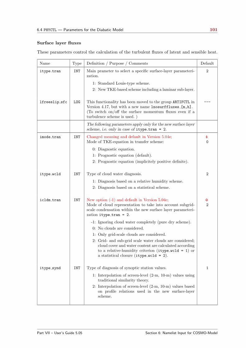
6.4 PHYCTL — Parameters for the Diabatic Model 101
Surface layer fluxes
These parameters control the calculation of the turbulent fluxes of latent and sensible heat.
Name Type Definition / Purpose / Comments Default
itype tran INT Main prameter to select a specific surface-layer parameteri-zation.
1: Standard Louis-type scheme.
2: New TKE-based scheme including a laminar sub-layer.
2
lfreeslip sfc LOG This functionality has been moved to the group ARTIFCTL inVersion 4.17, but with a new name lnosurffluxes [m,h].(To switch on/off the surface momentum fluxes even if aturbulence scheme is used. )
---
The following parameters apply only for the new surface layerscheme, i.e. only in case of itype tran = 2.
imode tran INT Changed meaning and default in Version 5.04e;Mode of TKE-equation in transfer scheme:
0: Diagnostic equation.
1: Prognostic equation (default).
2: Prognostic equation (implicitely positive definite).
1
0
itype wcld INT Type of cloud water diagnosis.
1: Diagnosis based on a relative humidity scheme.
2: Diagnosis based on a statistical scheme.
2
icldm tran INT New option (-1) and default in Version 5.04e;Mode of cloud representation to take into account subgrid-scale condensation within the new surface layer parameteri-zation itype tran = 2.
-1: Ignoring cloud water completely (pure dry scheme).
0: No clouds are considered.
1: Only grid-scale clouds are considered.
2: Grid- and sub-grid scale water clouds are considered;cloud cover and water content are calculated accordingto a relative-humidity criterion (itype wcld = 1) ora statistical closure (itype wcld = 2).
0
2
itype synd INT Type of diagnosis of synoptic station values.
1: Interpolation of screen-level (2-m, 10-m) values usingtraditional similarity theory.
2: Interpolation of screen-level (2-m, 10-m) values basedon profile relations used in the new surface-layerscheme.
1
Part VII – User’s Guide 5.05 Section 6: Namelist Input for COSMO-Model
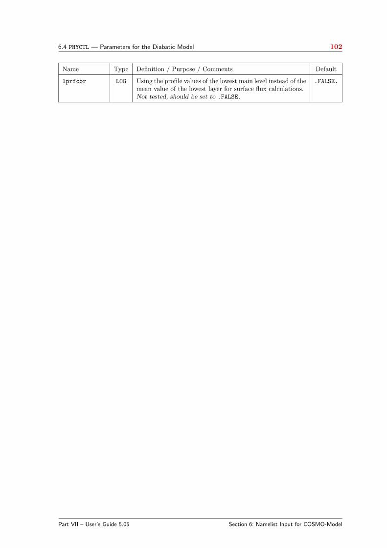
6.4 PHYCTL — Parameters for the Diabatic Model 102
Name Type Definition / Purpose / Comments Default
lprfcor LOG Using the profile values of the lowest main level instead of themean value of the lowest layer for surface flux calculations.Not tested, should be set to .FALSE.
.FALSE.
Part VII – User’s Guide 5.05 Section 6: Namelist Input for COSMO-Model
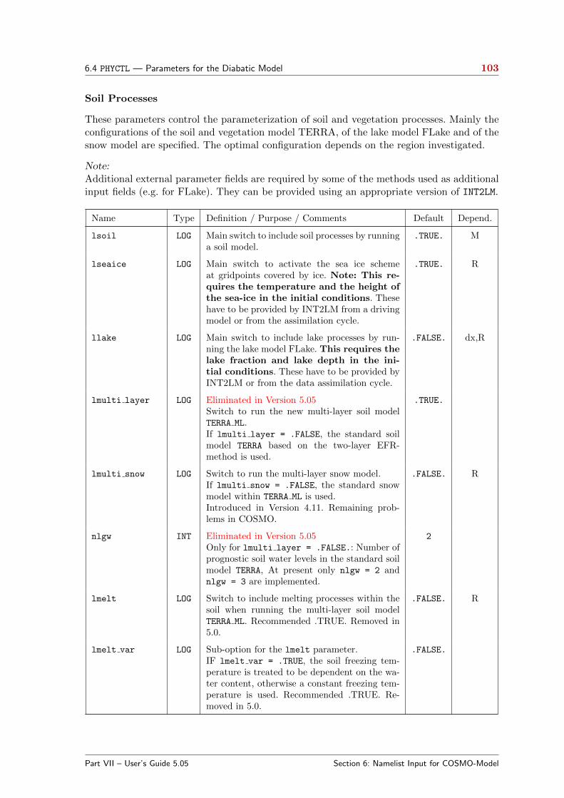
6.4 PHYCTL — Parameters for the Diabatic Model 103
Soil Processes
These parameters control the parameterization of soil and vegetation processes. Mainly theconfigurations of the soil and vegetation model TERRA, of the lake model FLake and of thesnow model are specified. The optimal configuration depends on the region investigated.
Note:Additional external parameter fields are required by some of the methods used as additionalinput fields (e.g. for FLake). They can be provided using an appropriate version of INT2LM.
Name Type Definition / Purpose / Comments Default Depend.
lsoil LOG Main switch to include soil processes by runninga soil model.
.TRUE. M
lseaice LOG Main switch to activate the sea ice schemeat gridpoints covered by ice. Note: This re-quires the temperature and the height ofthe sea-ice in the initial conditions. Thesehave to be provided by INT2LM from a drivingmodel or from the assimilation cycle.
.TRUE. R
llake LOG Main switch to include lake processes by run-ning the lake model FLake. This requires thelake fraction and lake depth in the ini-tial conditions. These have to be provided byINT2LM or from the data assimilation cycle.
.FALSE. dx,R
lmulti layer LOG Eliminated in Version 5.05Switch to run the new multi-layer soil modelTERRA ML.If lmulti layer = .FALSE, the standard soilmodel TERRA based on the two-layer EFR-method is used.
.TRUE.
lmulti snow LOG Switch to run the multi-layer snow model.If lmulti snow = .FALSE, the standard snowmodel within TERRA ML is used.Introduced in Version 4.11. Remaining prob-lems in COSMO.
.FALSE. R
nlgw INT Eliminated in Version 5.05Only for lmulti layer = .FALSE.: Number ofprognostic soil water levels in the standard soilmodel TERRA, At present only nlgw = 2 andnlgw = 3 are implemented.
2
lmelt LOG Switch to include melting processes within thesoil when running the multi-layer soil modelTERRA ML. Recommended .TRUE. Removed in5.0.
.FALSE. R
lmelt var LOG Sub-option for the lmelt parameter.IF lmelt var = .TRUE, the soil freezing tem-perature is treated to be dependent on the wa-ter content, otherwise a constant freezing tem-perature is used. Recommended .TRUE. Re-moved in 5.0.
.FALSE.
Part VII – User’s Guide 5.05 Section 6: Namelist Input for COSMO-Model
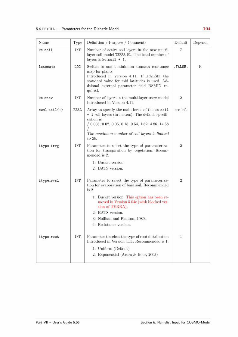
6.4 PHYCTL — Parameters for the Diabatic Model 104
Name Type Definition / Purpose / Comments Default Depend.
ke soil INT Number of active soil layers in the new multi-layer soil model TERRA ML. The total number oflayers is ke soil + 1.
7
lstomata LOG Switch to use a minimum stomata resistancemap for plantsIntroduced in Version 4.11.. If .FALSE. thestandard value for mid latitudes is used. Ad-dtional external parameter field RSMIN re-quired.
.FALSE. R
ke snow INT Number of layers in the multi-layer snow modelIntroduced in Version 4.11.
2
czml soil(:) REAL Array to specify the main levels of the ke soil
+ 1 soil layers (in meters). The default specifi-cation is/ 0.005, 0.02, 0.06, 0.18, 0.54, 1.62, 4.86, 14.58/The maximum number of soil layers is limitedto 20.
see left
itype trvg INT Parameter to select the type of parameteriza-tion for transpiration by vegetation. Recom-mended is 2.
1: Bucket version.
2: BATS version.
2
itype evsl INT Parameter to select the type of parameteriza-tion for evaporation of bare soil. Recommendedis 2.
1: Bucket version. This option has been re-moved in Version 5.04e (with blocked ver-sion of TERRA).
2: BATS version.
3: Noilhan and Planton, 1989.
4: Resistance version.
2
itype root INT Parameter to select the type of root distributionIntroduced in Version 4.11. Recommended is 1.
1: Uniform (Default)
2: Exponential (Arora & Boer, 2003)
1
Part VII – User’s Guide 5.05 Section 6: Namelist Input for COSMO-Model
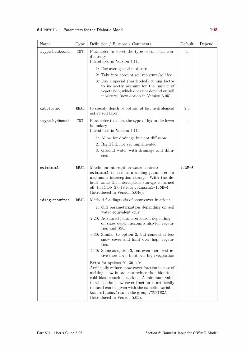
6.4 PHYCTL — Parameters for the Diabatic Model 105
Name Type Definition / Purpose / Comments Default Depend.
itype heatcond INT Parameter to select the type of soil heat con-ductivityIntroduced in Version 4.11.
1: Use average soil moisture
2: Take into account soil moisture/soil ice
3: Use a special (hardcoded) tuning factorto indirectly account for the impact ofvegetation, which does not depend on soilmoisture. (new option in Version 5.05).
1
czbot w so REAL to specify depth of bottom of last hydrologicalactive soil layer
2.5
itype hydbound INT Parameter to select the type of hydraulic lowerboundaryIntroduced in Version 4.11.
1: Allow for drainage but not diffusion
2: Rigid lid: not yet implemented
3: Ground water with drainage and diffu-sion
1
cwimax ml REAL Maximum interception water content:cwimax ml is used as a scaling parameter formaximum interception storage. With the de-fault value the interception storage is turnedoff. In ICON 2.0.18 it is cwimax ml=1.0E-4.(Introduced in Version 5.04e).
1.0E-6
idiag snowfrac REAL Method for diagnosis of snow-cover fraction:
1: Old parameterization depending on soilwater equivalent only.
2,20: Advanced parameterization dependingon snow depth, accounts also for vegeta-tion and SSO.
3,30: Similar to option 2, but somewhat lesssnow cover and limit over high vegeta-tion.
4,40: Same as option 3, but even more restric-tive snow cover limit over high vegetation
Extra for options 20, 30, 40:Artificially reduce snow-cover fraction in case ofmelting snow in order to reduce the ubiquitouscold bias in such situations. A minimum valueto which the snow cover fraction is artificiallyreduced can be given with the namelist variabletune minsnowfrac in the group /TUNING/.(Introduced in Version 5.05).
1
Part VII – User’s Guide 5.05 Section 6: Namelist Input for COSMO-Model
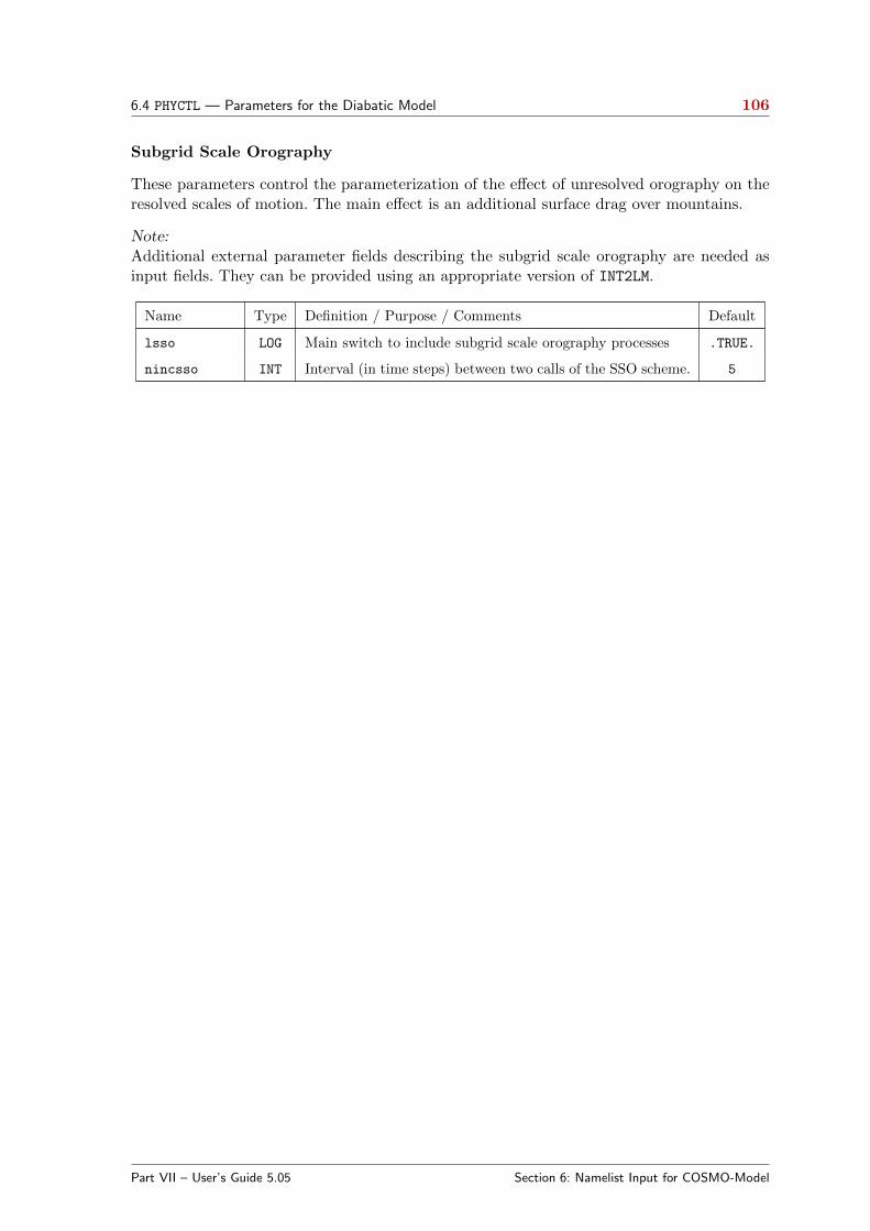
6.4 PHYCTL — Parameters for the Diabatic Model 106
Subgrid Scale Orography
These parameters control the parameterization of the effect of unresolved orography on theresolved scales of motion. The main effect is an additional surface drag over mountains.
Note:Additional external parameter fields describing the subgrid scale orography are needed asinput fields. They can be provided using an appropriate version of INT2LM.
Name Type Definition / Purpose / Comments Default
lsso LOG Main switch to include subgrid scale orography processes .TRUE.
nincsso INT Interval (in time steps) between two calls of the SSO scheme. 5
Part VII – User’s Guide 5.05 Section 6: Namelist Input for COSMO-Model
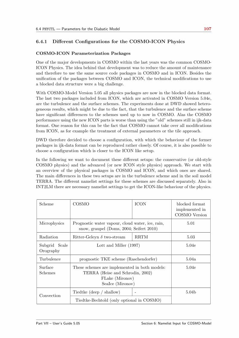
6.4 PHYCTL — Parameters for the Diabatic Model 107
6.4.1 Different Configurations for the COSMO-ICON Physics
COSMO-ICON Parameterization Packages
One of the major developments in COSMO within the last years was the common COSMO-ICON Physics. The idea behind that development was to reduce the amount of maintenanceand therefore to use the same source code packages in COSMO and in ICON. Besides theunification of the packages between COSMO and ICON, the technical modifications to usea blocked data structure were a big challenge.
With COSMO-Model Version 5.05 all physics packages are now in the blocked data format.The last two packages included from ICON, which are activated in COSMO Version 5.04e,are the turbulence and the surface schemes. The experiments done at DWD showed hetero-geneous results, which might be due to the fact, that the turbulence and the surface schemehave significant differences to the schemes used up to now in COSMO. Alas the COSMOperformance using the new ICON parts is worse than using the ”old” schemes still in ijk-dataformat. One reason for this can be the fact that COSMO cannot take over all modificationsfrom ICON, as for example the treatment of external parameters or the tile approach.
DWD therefore decided to choose a configuration, with which the behaviour of the formerpackages in ijk-data format can be reproduced rather closely. Of course, it is also possible tochoose a configuration which is closer to the ICON like setup.
In the following we want to document these different setups: the conservative (or old-styleCOSMO physics) and the advanced (or new ICON style physics) approach. We start withan overview of the physical packages in COSMO and ICON, and which ones are shared.The main differences in these two setups are in the turbulence scheme and in the soil modelTERRA. The different namelist settings for these schemes are discussed separately. Also inINT2LM there are necessary namelist settings to get the ICON-like behaviour of the physics.
Scheme COSMO ICON blocked formatimplemented in
COSMO Version
Microphysics Prognostic water vapour, cloud water, ice, rain,snow, graupel (Doms, 2004; Seifert 2010)
5.01
Radiation Ritter-Geleyn δ two-stream RRTM 5.03
Subgrid ScaleOrography
Lott and Miller (1997) 5.04e
Turbulence prognostic TKE scheme (Raschendorfer) 5.04a
SurfaceSchemes
These schemes are implemented in both models:TERRA (Heise and Schrodin, 2002)
FLake (Mironov)SeaIce (Mironov)
5.04e
ConvectionTiedtke (deep / shallow) - 5.04b
Tiedtke-Bechtold (only optional in COSMO)
Part VII – User’s Guide 5.05 Section 6: Namelist Input for COSMO-Model
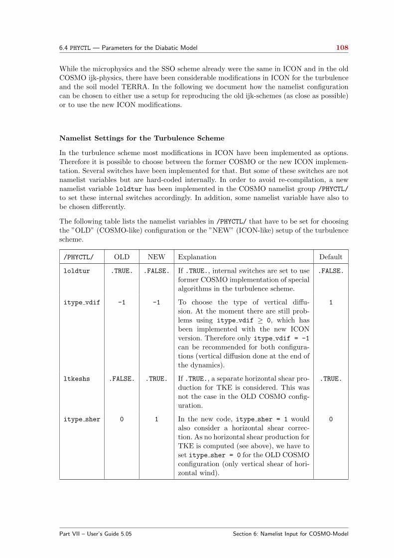
6.4 PHYCTL — Parameters for the Diabatic Model 108
While the microphysics and the SSO scheme already were the same in ICON and in the oldCOSMO ijk-physics, there have been considerable modifications in ICON for the turbulenceand the soil model TERRA. In the following we document how the namelist configurationcan be chosen to either use a setup for reproducing the old ijk-schemes (as close as possible)or to use the new ICON modifications.
Namelist Settings for the Turbulence Scheme
In the turbulence scheme most modifications in ICON have been implemented as options.Therefore it is possible to choose between the former COSMO or the new ICON implemen-tation. Several switches have been implemented for that. But some of these switches are notnamelist variables but are hard-coded internally. In order to avoid re-compilation, a newnamelist variable loldtur has been implemented in the COSMO namelist group /PHYCTL/
to set these internal switches accordingly. In addition, some namelist variable have also tobe chosen differently.
The following table lists the namelist variables in /PHYCTL/ that have to be set for choosingthe ”OLD” (COSMO-like) configuration or the ”NEW” (ICON-like) setup of the turbulencescheme.
/PHYCTL/ OLD NEW Explanation Default
loldtur .TRUE. .FALSE. If .TRUE., internal switches are set to useformer COSMO implementation of specialalgorithms in the turbulence scheme.
.FALSE.
itype vdif -1 -1 To choose the type of vertical diffu-sion. At the moment there are still prob-lems using itype vdif ≥ 0, which hasbeen implemented with the new ICONversion. Therefore only itype vdif = -1
can be recommended for both configura-tions (vertical diffusion done at the end ofthe dynamics).
1
ltkeshs .FALSE. .TRUE. If .TRUE., a separate horizontal shear pro-duction for TKE is considered. This wasnot the case in the OLD COSMO config-uration.
.TRUE.
itype sher 0 1 In the new code, itype sher = 1 wouldalso consider a horizontal shear correc-tion. As no horizontal shear production forTKE is computed (see above), we have toset itype sher = 0 for the OLD COSMOconfiguration (only vertical shear of hori-zontal wind).
0
Part VII – User’s Guide 5.05 Section 6: Namelist Input for COSMO-Model
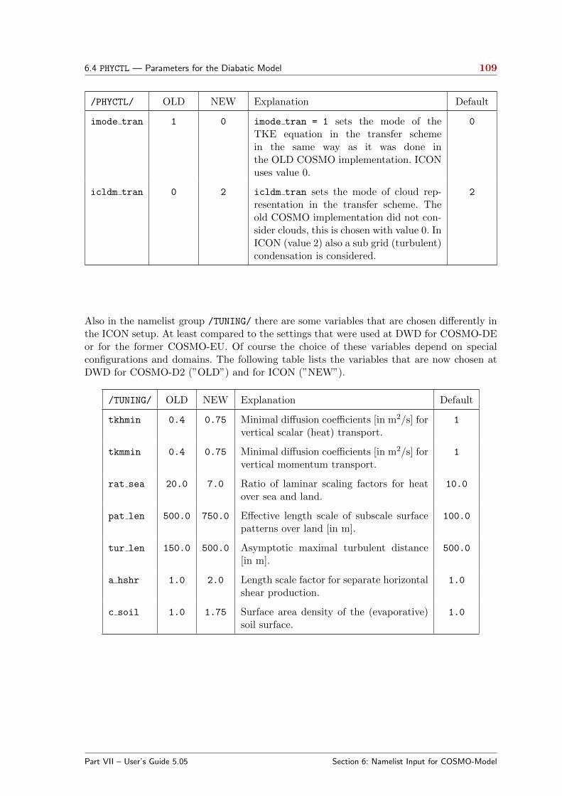
6.4 PHYCTL — Parameters for the Diabatic Model 109
/PHYCTL/ OLD NEW Explanation Default
imode tran 1 0 imode tran = 1 sets the mode of theTKE equation in the transfer schemein the same way as it was done inthe OLD COSMO implementation. ICONuses value 0.
0
icldm tran 0 2 icldm tran sets the mode of cloud rep-resentation in the transfer scheme. Theold COSMO implementation did not con-sider clouds, this is chosen with value 0. InICON (value 2) also a sub grid (turbulent)condensation is considered.
2
Also in the namelist group /TUNING/ there are some variables that are chosen differently inthe ICON setup. At least compared to the settings that were used at DWD for COSMO-DEor for the former COSMO-EU. Of course the choice of these variables depend on specialconfigurations and domains. The following table lists the variables that are now chosen atDWD for COSMO-D2 (”OLD”) and for ICON (”NEW”).
/TUNING/ OLD NEW Explanation Default
tkhmin 0.4 0.75 Minimal diffusion coefficients [in m2/s] forvertical scalar (heat) transport.
1
tkmmin 0.4 0.75 Minimal diffusion coefficients [in m2/s] forvertical momentum transport.
1
rat sea 20.0 7.0 Ratio of laminar scaling factors for heatover sea and land.
10.0
pat len 500.0 750.0 Effective length scale of subscale surfacepatterns over land [in m].
100.0
tur len 150.0 500.0 Asymptotic maximal turbulent distance[in m].
500.0
a hshr 1.0 2.0 Length scale factor for separate horizontalshear production.
1.0
c soil 1.0 1.75 Surface area density of the (evaporative)soil surface.
1.0
Part VII – User’s Guide 5.05 Section 6: Namelist Input for COSMO-Model

6.4 PHYCTL — Parameters for the Diabatic Model 110
Namelist Settings for TERRA
Also in TERRA there have been considerable changes in the ICON version compared tothe OLD COSMO implementation. Most of these modifications are not optional, so there isno way to mimic the OLD behaviour. Only for some algorithms, which already had severaloptions, new ways have been implemented, which could be chosen now. Note that not allICON options can be used in COSMO due to a different treatment of external parametersand the ICON tile approach.
The following table lists the namelist variables with which new ICON options could be chosen.The column ”OLD” again lists the COSMO-D2 settings from DWD, which correspond tothe former configuration of TERRA, while the column ”NEW” lists the ICON settings.DWD did not make enough tests (independent from the turbulence settings) to judge theperformance of the ICON settings in COSMO. But everybody is free to do so!
/TUNING/ OLD NEW Explanation Default
itype evsl 2 4 Type of parameterization of bare soilevaporation. Option 4 is the new imple-mentation by Jan-Peter Schulz. Notethat option 1 is no more available.
2
itype heatcond 1 3 Type of soil heat conductivity: Option1 uses an average soil moisture. Newoption 3 uses a special (hardcoded)tuning factor to indirectly account forthe impact of vegetation, which doesnot depend on soil moisture.
1
itype root 1 2 Type of root distribution: Option 1 as-sumes a uniform distribution used inthe OLD COSMO configuration. Op-tion 2, which assumes an exponentialdistribution, is used in ICON. Pleasenote, that if you want to use option 2,you also have to use itype rootdp =
4 in the INT2LM!
1
cwimax ml 1.0E-6 0.0005 cwimax ml is used as a scaling parame-ter for maximum interception storage.In the OLD COSMO implementationthis was a constant with value 1.0E-6. Now it is a namelist variable. ICONuses a value of 5.0E-4 = 0.0005.
1.0E-6
itype snowfrac 1 20 Method for diagnosis of snow-coverfraction. (Further explanation neces-sary).
1
Part VII – User’s Guide 5.05 Section 6: Namelist Input for COSMO-Model
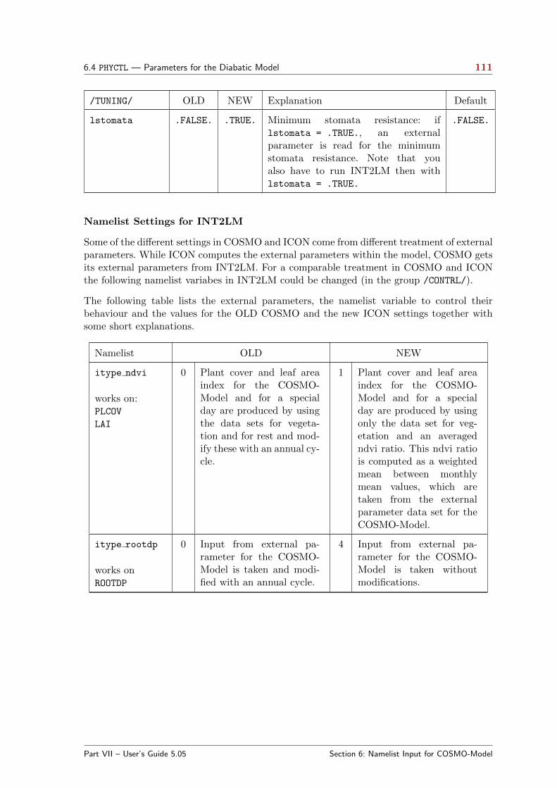
6.4 PHYCTL — Parameters for the Diabatic Model 111
/TUNING/ OLD NEW Explanation Default
lstomata .FALSE. .TRUE. Minimum stomata resistance: iflstomata = .TRUE., an externalparameter is read for the minimumstomata resistance. Note that youalso have to run INT2LM then withlstomata = .TRUE.
.FALSE.
Namelist Settings for INT2LM
Some of the different settings in COSMO and ICON come from different treatment of externalparameters. While ICON computes the external parameters within the model, COSMO getsits external parameters from INT2LM. For a comparable treatment in COSMO and ICONthe following namelist variabes in INT2LM could be changed (in the group /CONTRL/).
The following table lists the external parameters, the namelist variable to control theirbehaviour and the values for the OLD COSMO and the new ICON settings together withsome short explanations.
Namelist OLD NEW
itype ndvi
works on:PLCOV
LAI
0 Plant cover and leaf areaindex for the COSMO-Model and for a specialday are produced by usingthe data sets for vegeta-tion and for rest and mod-ify these with an annual cy-cle.
1 Plant cover and leaf areaindex for the COSMO-Model and for a specialday are produced by usingonly the data set for veg-etation and an averagedndvi ratio. This ndvi ratiois computed as a weightedmean between monthlymean values, which aretaken from the externalparameter data set for theCOSMO-Model.
itype rootdp
works onROOTDP
0 Input from external pa-rameter for the COSMO-Model is taken and modi-fied with an annual cycle.
4 Input from external pa-rameter for the COSMO-Model is taken withoutmodifications.
Part VII – User’s Guide 5.05 Section 6: Namelist Input for COSMO-Model

6.4 PHYCTL — Parameters for the Diabatic Model 112
Namelist OLD NEW
itype aerosol
works onAER SO4
AER DUST
AER ORG
AER BC
AER SS
1 No additional Fields foraerosol types are read fromthe external parameters.The COSMO-Model has torun with constant valuesfor the aerosol distributionon rural areas, urban ar-eas, desert areas or thesea (Tanre aerosol clima-tology).
2 Additional external pa-rameters for the aerosoltypes of sulfate, min-eral dust, organic, blackcarbon and sea salt areread as monthly meanvalues. Actual values forthe current day are com-puted and given to theCOSMO-Model (Tegenaerosol climatology).
lstomata
works onRSMIN
.FALSE.
No external parameter istaken. A constant valuefor all grid points is de-termined in the COSMO-Model.
.TRUE.
Take a map from the exter-nal parameters for the min-imum stomata resistance ofplants.
lemiss
works onEMIS RAD
.FALSE.
No external parameter istaken. A constant valuefor all grid points is de-termined in the COSMO-Model.
.TRUE.
Take a map from the ex-ternal parameters for thethermal radiative surfaceemissivity.
NOTE: Usage of SSO STDH and SSO SIGMA:
The new turbulence scheme now needs the external parameter SSO STDH and the new schemefor TERRA needs SSO SIGMA. Therefore the namelist variable lsso should be set to .TRUE.
in any case when running INT2LM.
Part VII – User’s Guide 5.05 Section 6: Namelist Input for COSMO-Model
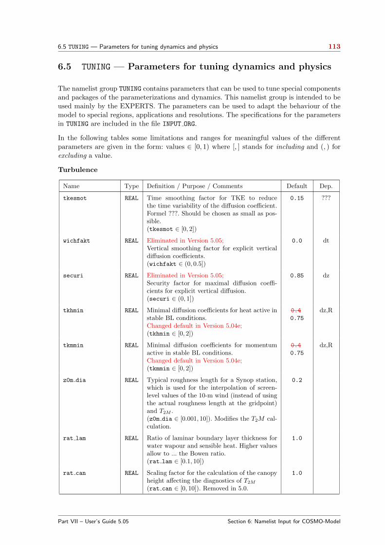
6.5 TUNING — Parameters for tuning dynamics and physics 113
6.5 TUNING — Parameters for tuning dynamics and physics
The namelist group TUNING contains parameters that can be used to tune special componentsand packages of the parameterizations and dynamics. This namelist group is intended to beused mainly by the EXPERTS. The parameters can be used to adapt the behaviour of themodel to special regions, applications and resolutions. The specifications for the parametersin TUNING are included in the file INPUT ORG.
In the following tables some limitations and ranges for meaningful values of the differentparameters are given in the form: values ∈ [0, 1) where [, ] stands for including and (, ) forexcluding a value.
Turbulence
Name Type Definition / Purpose / Comments Default Dep.
tkesmot REAL Time smoothing factor for TKE to reducethe time variability of the diffusion coefficient.Formel ???. Should be chosen as small as pos-sible.(tkesmot ∈ [0, 2])
0.15 ???
wichfakt REAL Eliminated in Version 5.05;Vertical smoothing factor for explicit verticaldiffusion coefficients.(wichfakt ∈ (0, 0.5])
0.0 dt
securi REAL Eliminated in Version 5.05;Security factor for maximal diffusion coeffi-cients for explicit vertical diffusion.(securi ∈ (0, 1])
0.85 dz
tkhmin REAL Minimal diffusion coefficients for heat active instable BL conditions.Changed default in Version 5.04e;(tkhmin ∈ [0, 2])
0.4
0.75
dz,R
tkmmin REAL Minimal diffusion coefficients for momentumactive in stable BL conditions.Changed default in Version 5.04e;(tkmmin ∈ [0, 2])
0.4
0.75
dz,R
z0m dia REAL Typical roughness length for a Synop station,which is used for the interpolation of screen-level values of the 10-m wind (instead of usingthe actual roughness length at the gridpoint)and T2M .(z0m dia ∈ [0.001, 10]). Modifies the T2M cal-culation.
0.2
rat lam REAL Ratio of laminar boundary layer thickness forwater wapour and sensible heat. Higher valuesallow to ... the Bowen ratio.(rat lam ∈ [0.1, 10])
1.0
rat can REAL Scaling factor for the calculation of the canopyheight affecting the diagnostics of T2M
(rat can ∈ [0, 10]). Removed in 5.0.
1.0
Part VII – User’s Guide 5.05 Section 6: Namelist Input for COSMO-Model
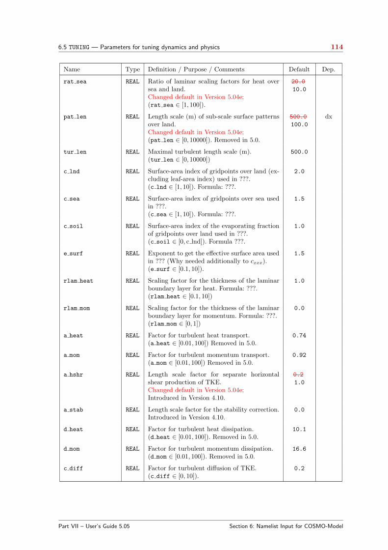
6.5 TUNING — Parameters for tuning dynamics and physics 114
Name Type Definition / Purpose / Comments Default Dep.
rat sea REAL Ratio of laminar scaling factors for heat oversea and land.Changed default in Version 5.04e;(rat sea ∈ [1, 100]).
20.0
10.0
pat len REAL Length scale (m) of sub-scale surface patternsover land.Changed default in Version 5.04e;(pat len ∈ [0, 10000]). Removed in 5.0.
500.0
100.0
dx
tur len REAL Maximal turbulent length scale (m).(tur len ∈ [0, 10000])
500.0
c lnd REAL Surface-area index of gridpoints over land (ex-cluding leaf-area index) used in ???.(c lnd ∈ [1, 10]). Formula: ???.
2.0
c sea REAL Surface-area index of gridpoints over sea usedin ???.(c sea ∈ [1, 10]). Formula: ???.
1.5
c soil REAL Surface-area index of the evaporating fractionof gridpoints over land used in ???.(c soil ∈ [0, c lnd]). Formula ???.
1.0
e surf REAL Exponent to get the effective surface area usedin ??? (Why needed additionally to cxxx).(e surf ∈ [0.1, 10]).
1.5
rlam heat REAL Scaling factor for the thickness of the laminarboundary layer for heat. Formula: ???.(rlam heat ∈ [0.1, 10])
1.0
rlam mom REAL Scaling factor for the thickness of the laminarboundary layer for momentum. Formula: ???.(rlam mom ∈ [0, 1])
0.0
a heat REAL Factor for turbulent heat transport.(a heat ∈ [0.01, 100]) Removed in 5.0.
0.74
a mom REAL Factor for turbulent momentum transport.(a mom ∈ [0.01, 100]) Removed in 5.0.
0.92
a hshr REAL Length scale factor for separate horizontalshear production of TKE.Changed default in Version 5.04e;Introduced in Version 4.10.
0.2
1.0
a stab REAL Length scale factor for the stability correction.Introduced in Version 4.10.
0.0
d heat REAL Factor for turbulent heat dissipation.(d heat ∈ [0.01, 100]). Removed in 5.0.
10.1
d mom REAL Factor for turbulent momentum dissipation.(d mom ∈ [0.01, 100]). Removed in 5.0.
16.6
c diff REAL Factor for turbulent diffusion of TKE.(c diff ∈ [0, 10]).
0.2
Part VII – User’s Guide 5.05 Section 6: Namelist Input for COSMO-Model

6.5 TUNING — Parameters for tuning dynamics and physics 115
Name Type Definition / Purpose / Comments Default Dep.
clc diag REAL Cloud cover at saturation in statistical clouddiagnostic.(clc diag ∈ (0, 1))
0.5
q crit REAL Critical value for normalized over-saturation.(q crit ∈ [1, 10])
4.0
Surface Schemes
Name Type Definition / Purpose / Comments Default Dep.
crsmin REAL Minimum value of stomatal resistance (used bythe BATS approach for vegetation transpira-tion, itype trvg=2).(crsmin ∈ [50, 200])
150.0
tune minsnowfrac REAL In case of melting snow the snow cover fractionis artificially reduced to this minimum value (incombination with idiag snowfrac = 20/30/40in group /PHYCTL/).(Introduced in Version 5.05).
0.125
SSO Scheme
Name Type Definition / Purpose / Comments Default Dep.
gkdrag REAL Scaling factor for gravity wave drag in SSOscheme.Reasonable values are: gkdrag ∈ [0.0, 1.0].With a value of 1, the gravity wave drag in theSSO scheme is switched on. When reducing thevalue, the strength of the gravity wave drag isreduced. With a value of 0, the gravity wavedrag in the SSO scheme is switched off.
0.075
gkwake REAL Scaling factor for low-level flow blocking inSSO scheme.Reasonable values are: gkwake ∈ [0.0, 1.0].With a value of 1, the low-level flow blockingin the SSO scheme is switched on. When re-ducing the value, the strength of the low-levelflow blocking is reduced. With a value of 0, thelow-level flow blocking in the SSO scheme isswitched off.
0.5
Part VII – User’s Guide 5.05 Section 6: Namelist Input for COSMO-Model

6.5 TUNING — Parameters for tuning dynamics and physics 116
Radiation
Name Type Definition / Purpose / Comments Default Dep.
radqc fact REAL Portion of grid scale qc + qr seen by the ra-diation.Reasonable values are:radqc fact ∈ [0.5, 1.0].(Introduced in Version 5.04c).
0.5
radqi fact REAL Portion of grid scale qi + qs + qg seen by theradiation.Reasonable values are: radqi fact ∈ [0.5, 1.0].(Introduced in Version 5.04c).
0.5
Microphysics
Name Type Definition / Purpose / Comments Default Dep.
qc0 REAL Cloud water threshold for autoconversion. 0.0
qi0 REAL Cloud ice threshold for autoconversion. 0.0
mu rain REAL Shape parameter of the rain drop size distribu-tion.Reasonable values are: mu rain ∈ [0.0, 5.0].Introduced in Version 4.5.ATTENTION: In Version 4.21 the defaultvalue has been changed from 0.5 to 0.0!
0.0
rain n0 factor REAL To reduce the evaporation of rain drops.Reasonable values are:rain n0 factor ∈ [0.0, 1.0].Introduced in Version 4.14.
1.0
cloud num REAL Cloud droplet number concentration. 5.0
E+08
v0snow REAL Factor in the terminal velocity for snow.This was a local variable in the subroutineshydci pp and hydci pp gr before, but had dif-ferent values. To reproduce the results from theformer version, the following values have to beset:
itype gscp = 3 and LF: 15.0
itype gscp = 3 and RK: 25.0
itype gscp = 4 and RK: 20.0
Introduced in Version 4.14.
25.0
Part VII – User’s Guide 5.05 Section 6: Namelist Input for COSMO-Model
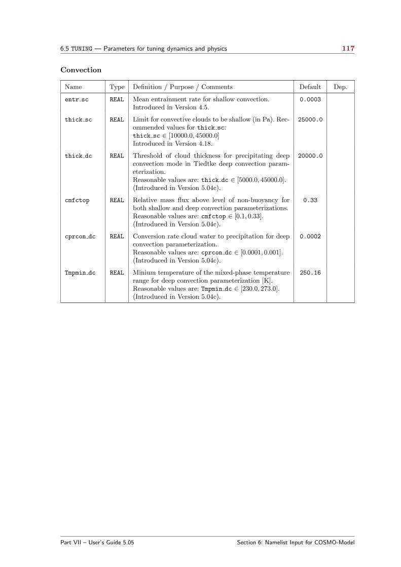
6.5 TUNING — Parameters for tuning dynamics and physics 117
Convection
Name Type Definition / Purpose / Comments Default Dep.
entr sc REAL Mean entrainment rate for shallow convection.Introduced in Version 4.5.
0.0003
thick sc REAL Limit for convective clouds to be shallow (in Pa). Rec-ommended values for thick sc:thick sc ∈ [10000.0, 45000.0]Introduced in Version 4.18.
25000.0
thick dc REAL Threshold of cloud thickness for precipitating deepconvection mode in Tiedtke deep convection param-eterization.Reasonable values are: thick dc ∈ [5000.0, 45000.0].(Introduced in Version 5.04c).
20000.0
cmfctop REAL Relative mass flux above level of non-buoyancy forboth shallow and deep convection parameterizations.Reasonable values are: cmfctop ∈ [0.1, 0.33].(Introduced in Version 5.04c).
0.33
cprcon dc REAL Conversion rate cloud water to precipitation for deepconvection parameterization.Reasonable values are: cprcon dc ∈ [0.0001, 0.001].(Introduced in Version 5.04c).
0.0002
Tmpmin dc REAL Minium temperature of the mixed-phase temperaturerange for deep convection parameterization [K].Reasonable values are: Tmpmin dc ∈ [230.0, 273.0].(Introduced in Version 5.04c).
250.16
Part VII – User’s Guide 5.05 Section 6: Namelist Input for COSMO-Model

6.5 TUNING — Parameters for tuning dynamics and physics 118
Additional switches only for Tiedtke-Bechtold scheme
These switches have been introduced with version 5.04b, when the Tiedtke-Bechtold schemehas been implemented.
Name Type Definition / Purpose / Comments Default
tune capdcfac et REAL Fraction of CAPE diurnal cycle correction ap-plied in the extratropics.
0.0
tune rhebc land REAL Relative humidity threshold for onset of evapora-tion below cloud base over land.
0.75
tune rhebc ocean REAL Relative humidity threshold for onset of evapora-tion below cloud base over sea.
0.85
tune texc REAL Excess value for temperature used in test parcelascent.
0.125
tune qexc REAL Excess fraction of grid-scale QV used in test par-cel ascent.
0.0125
tune rcucov REAL Convective area fraction. 0.05
tune entrorg REAL Entrainment parameter for deep convection validat dx=20 km.
0.001825
tune rhebc land trop REAL Relative humidity threshold for onset of evapora-tion below cloud base over land in the tropics.
0.7
tune rhebc ocean trop REAL Relative humidity threshold for onset of evapora-tion below cloud base over sea in the tropics.
0.8
tune rcucov trop REAL Convective area fraction in the tropics. 0.05
Part VII – User’s Guide 5.05 Section 6: Namelist Input for COSMO-Model

6.6 DIACTL — Parameters for Diagnostic Output 119
6.6 DIACTL — Parameters for Diagnostic Output
DIACTL contains parameters to generate gridpoint and control ASCII output. These param-eters are only in effect if the main switch ldiagnos in RUNCTL is set to .TRUE.. In thiscase, some additional time integrated fields – TDIV HUM (vertically integrated divergence ofspecific humidity) and AEVAP S (surface moisture flux) – are also calculated to allow for amass-budget calculation based on GRIB-output. Currently, the following ASCII output canbe generated:
- Grid point output (meteographs) in a specific form;results are written to files M stationname.
- Control output for a quick-look monitoring of the model run;results are written to files YUPRMASS (for mass variables) and YUPRHUMI (for humidityvariables), resp.
Note: Up to model version 3.4, two addtional forms of ASCII output could be generated: Di-agnostics for various subdomains and differences between predicted and and boundary fields.Since these diagnostics can be easily calculated from GRIB-output, they will no longer beretained.
See Part VI of the COSMO-Model Documentation (Model Output and Data Formats forI/O for a further description of the ASCII output.
Parameters for control ouput
For control output, a number of variables are computed and written to the ASCII filesYUPRMASS (for mass variables) and YUPRHUMI (for humidity variables). These variables aredomain averages of quantities like surface pressure, surface pressure tendency, kinetic energy,dry static energy, moist static energy, cloud water content, absolute vertical velocity at certainlevels, precipitation rates and accumulated precipitation, and domain maxima of absolutehorizontal and vertical velocity. This allows for a quick-look control of the model run.
Name Type Definition / Purpose / Comments Default
n0meanval INT Number of time step for the first call of control output. Ifn0meanval > nstop, no control output will be computed.
0
nincmeanval INT Interval (in time steps) between two calls of the control cal-culations.
10
Ouput for COSMO Testsuite
Name Type Definition / Purpose / Comments Default
ltestsuite LOG To activate additional ASCII output, which is used and eval-uated when running the COSMO Technical Testsuite.
.FALSE.
Part VII – User’s Guide 5.05 Section 6: Namelist Input for COSMO-Model
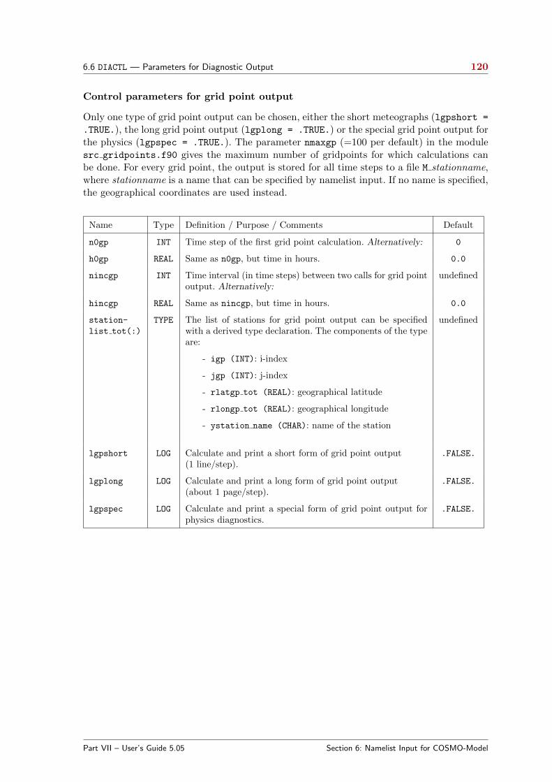
6.6 DIACTL — Parameters for Diagnostic Output 120
Control parameters for grid point output
Only one type of grid point output can be chosen, either the short meteographs (lgpshort =
.TRUE.), the long grid point output (lgplong = .TRUE.) or the special grid point output forthe physics (lgpspec = .TRUE.). The parameter nmaxgp (=100 per default) in the modulesrc gridpoints.f90 gives the maximum number of gridpoints for which calculations canbe done. For every grid point, the output is stored for all time steps to a file M stationname,where stationname is a name that can be specified by namelist input. If no name is specified,the geographical coordinates are used instead.
Name Type Definition / Purpose / Comments Default
n0gp INT Time step of the first grid point calculation. Alternatively: 0
h0gp REAL Same as n0gp, but time in hours. 0.0
nincgp INT Time interval (in time steps) between two calls for grid pointoutput. Alternatively:
undefined
hincgp REAL Same as nincgp, but time in hours. 0.0
station-
list tot(:)
TYPE The list of stations for grid point output can be specifiedwith a derived type declaration. The components of the typeare:
- igp (INT): i-index
- jgp (INT): j-index
- rlatgp tot (REAL): geographical latitude
- rlongp tot (REAL): geographical longitude
- ystation name (CHAR): name of the station
undefined
lgpshort LOG Calculate and print a short form of grid point output(1 line/step).
.FALSE.
lgplong LOG Calculate and print a long form of grid point output(about 1 page/step).
.FALSE.
lgpspec LOG Calculate and print a special form of grid point output forphysics diagnostics.
.FALSE.
Part VII – User’s Guide 5.05 Section 6: Namelist Input for COSMO-Model
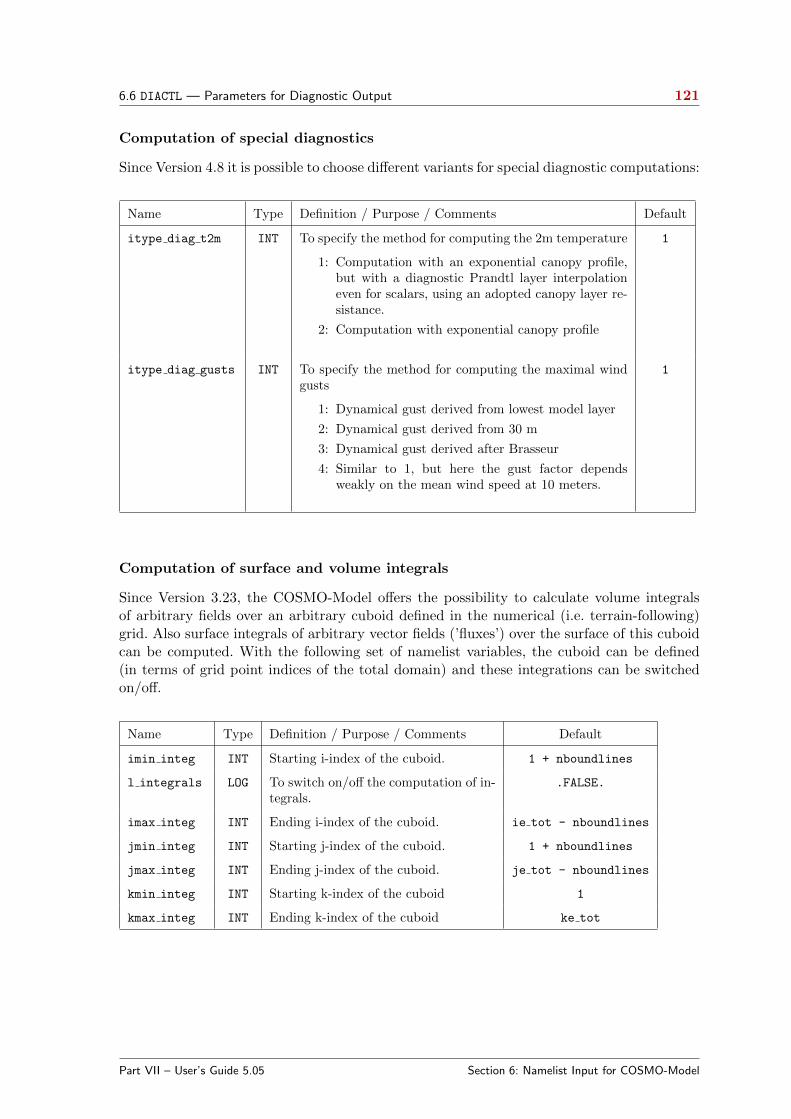
6.6 DIACTL — Parameters for Diagnostic Output 121
Computation of special diagnostics
Since Version 4.8 it is possible to choose different variants for special diagnostic computations:
Name Type Definition / Purpose / Comments Default
itype diag t2m INT To specify the method for computing the 2m temperature
1: Computation with an exponential canopy profile,but with a diagnostic Prandtl layer interpolationeven for scalars, using an adopted canopy layer re-sistance.
2: Computation with exponential canopy profile
1
itype diag gusts INT To specify the method for computing the maximal windgusts
1: Dynamical gust derived from lowest model layer
2: Dynamical gust derived from 30 m
3: Dynamical gust derived after Brasseur
4: Similar to 1, but here the gust factor dependsweakly on the mean wind speed at 10 meters.
1
Computation of surface and volume integrals
Since Version 3.23, the COSMO-Model offers the possibility to calculate volume integralsof arbitrary fields over an arbitrary cuboid defined in the numerical (i.e. terrain-following)grid. Also surface integrals of arbitrary vector fields (’fluxes’) over the surface of this cuboidcan be computed. With the following set of namelist variables, the cuboid can be defined(in terms of grid point indices of the total domain) and these integrations can be switchedon/off.
Name Type Definition / Purpose / Comments Default
imin integ INT Starting i-index of the cuboid. 1 + nboundlines
l integrals LOG To switch on/off the computation of in-tegrals.
.FALSE.
imax integ INT Ending i-index of the cuboid. ie tot - nboundlines
jmin integ INT Starting j-index of the cuboid. 1 + nboundlines
jmax integ INT Ending j-index of the cuboid. je tot - nboundlines
kmin integ INT Starting k-index of the cuboid 1
kmax integ INT Ending k-index of the cuboid ke tot
Part VII – User’s Guide 5.05 Section 6: Namelist Input for COSMO-Model
6.7 SATCTL — Controlling the Synthetic Satellite Images 122
6.7 SATCTL — Controlling the Synthetic Satellite Images
In August 2003 a project was started between DWD and the DLR Institute for AtmosphericPhysics which aimed at the generation of synthetic satellite images within the COSMO-Model. The RTTOV (Radiative Transfer model for TIROS Operational Vertical sounder)model, Version 7, is used to compute radiances for satellite infrared or microwave nadir scan-ning radiometers from an atmospheric profile of temperature, variable gas concentrations,and cloud and surface properties.
From Version 4.18 up to Version 5.04e, also the use of RTTOV, Version 9, was possible, buthas been removed again.
From Version 4.26 on, RTTOV 10 can be used. And in Version 5.05 also RTTOV 12 hasbeen implemented.
The different RTTOV-libraries are included in the COSMO-Model by conditional compila-tion. Depending on which implementation is used, the corresponding macro has to be setwhen compiling the COSMO-Model (for example with -DRTTOV7):
’RTTOV7’ to use the RTTOV7 library.Note that the COSMO-Model does not use the official RTTOV7 library, but a modifiedone, which takes care of using this library within parallel programs. It also containssome optimizations for vector processors.
’RTTOV9’ to use the RTTOV9 library. Eliminated in Version 5.05.
’RTTOV10’ to use the RTTOV10 library.
’RTTOV12’ to use the RTTOV12 library.
To use RTTOV10 or RTTOV12, another module, developed at DWD, is necessary as interfaceto this library: mo rttov ifc.f90. This module is available from DWD.
The RTTOV model can compute radiances and brightness temperatures of several instru-ments, which are located on diverse satellites. The implementation provided in the COSMO-Model only can compute the values for the following two instruments and channels specifiedin Table 6.38.
For every channel the following 4 products can be computed:
• cloudy brightness temperature
• clear-sky brightness temperature
• cloudy radiance
• clear-sky radiance
Note that the values for METEOSAT satellites can be computed, but be aware of the locationof these satellites. Only MSG 2 is located such that it is useful for Europe.
Part VII – User’s Guide 5.05 Section 6: Namelist Input for COSMO-Model
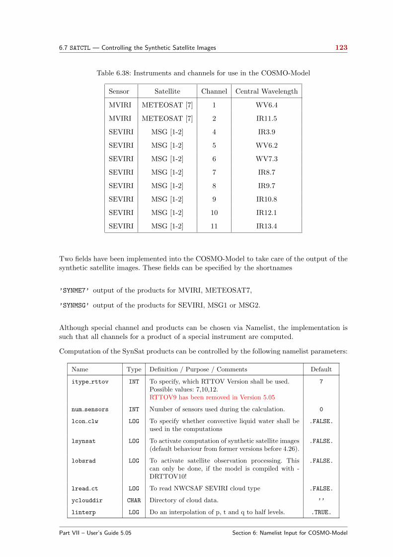
6.7 SATCTL — Controlling the Synthetic Satellite Images 123
Table 6.38: Instruments and channels for use in the COSMO-Model
Sensor Satellite Channel Central Wavelength
MVIRI METEOSAT [7] 1 WV6.4
MVIRI METEOSAT [7] 2 IR11.5
SEVIRI MSG [1-2] 4 IR3.9
SEVIRI MSG [1-2] 5 WV6.2
SEVIRI MSG [1-2] 6 WV7.3
SEVIRI MSG [1-2] 7 IR8.7
SEVIRI MSG [1-2] 8 IR9.7
SEVIRI MSG [1-2] 9 IR10.8
SEVIRI MSG [1-2] 10 IR12.1
SEVIRI MSG [1-2] 11 IR13.4
Two fields have been implemented into the COSMO-Model to take care of the output of thesynthetic satellite images. These fields can be specified by the shortnames
’SYNME7’ output of the products for MVIRI, METEOSAT7,
’SYNMSG’ output of the products for SEVIRI, MSG1 or MSG2.
Although special channel and products can be chosen via Namelist, the implementation issuch that all channels for a product of a special instrument are computed.
Computation of the SynSat products can be controlled by the following namelist parameters:
Name Type Definition / Purpose / Comments Default
itype rttov INT To specify, which RTTOV Version shall be used.Possible values: 7,10,12.RTTOV9 has been removed in Version 5.05
7
num sensors INT Number of sensors used during the calculation. 0
lcon clw LOG To specify whether convective liquid water shall beused in the computations
.FALSE.
lsynsat LOG To activate computation of synthetic satellite images(default behaviour from former versions before 4.26).
.FALSE.
lobsrad LOG To activate satellite observation processing. Thiscan only be done, if the model is compiled with -DRTTOV10!
.FALSE.
lread ct LOG To read NWCSAF SEVIRI cloud type .FALSE.
yclouddir CHAR Directory of cloud data. ’’
linterp LOG Do an interpolation of p, t and q to half levels. .TRUE.
Part VII – User’s Guide 5.05 Section 6: Namelist Input for COSMO-Model
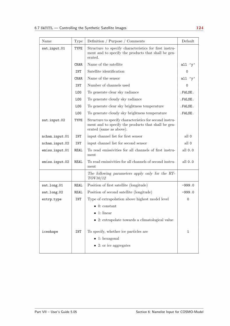
6.7 SATCTL — Controlling the Synthetic Satellite Images 124
Name Type Definition / Purpose / Comments Default
sat input 01 TYPE Structure to specify characteristics for first instru-ment and to specify the products that shall be gen-erated.
CHAR Name of the satellite all ’y’
INT Satellite identification 0
CHAR Name of the sensor all ’y’
INT Number of channels used 0
LOG To generate clear sky radiance .FALSE.
LOG To generate cloudy sky radiance .FALSE.
LOG To generate clear sky brightness temperature .FALSE.
LOG To generate cloudy sky brightness temperature .FALSE.
sat input 02 TYPE Structure to specify characteristics for second instru-ment and to specify the products that shall be gen-erated (same as above).
nchan input 01 INT input channel list for first sensor all 0
nchan input 02 INT input channel list for second sensor all 0
emiss input 01 REAL To read emissivities for all channels of first instru-ment
all 0.0
emiss input 02 REAL To read emissivities for all channels of second instru-ment
all 0.0
The following parameters apply only for the RT-TOV10/12
sat long 01 REAL Position of first satellite (longitude) -999.0
sat long 02 REAL Position of second satellite (longitude) -999.0
extrp type INT Type of extrapolation above highest model level
• 0: constant
• 1: linear
• 2: extrapolate towards a climatological value
0
iceshape INT To specify, whether ice particles are
• 1: hexagonal
• 2: or ice aggregates
1
Part VII – User’s Guide 5.05 Section 6: Namelist Input for COSMO-Model
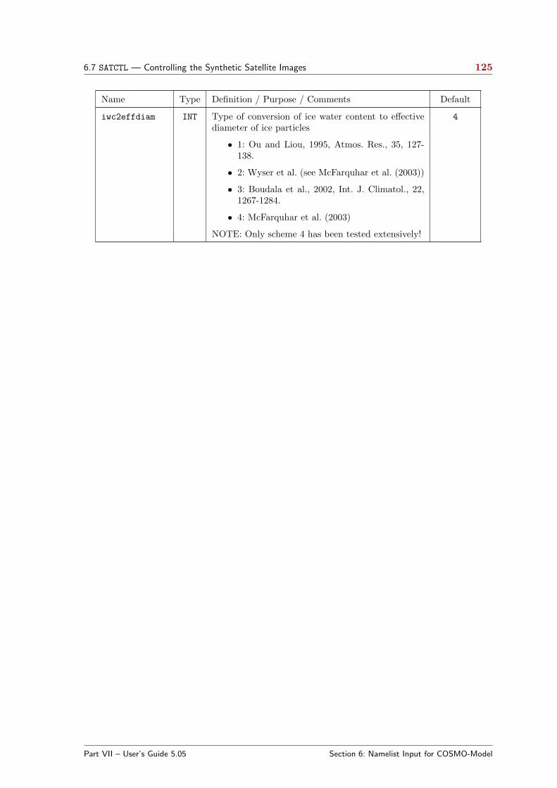
6.7 SATCTL — Controlling the Synthetic Satellite Images 125
Name Type Definition / Purpose / Comments Default
iwc2effdiam INT Type of conversion of ice water content to effectivediameter of ice particles
• 1: Ou and Liou, 1995, Atmos. Res., 35, 127-138.
• 2: Wyser et al. (see McFarquhar et al. (2003))
• 3: Boudala et al., 2002, Int. J. Climatol., 22,1267-1284.
• 4: McFarquhar et al. (2003)
NOTE: Only scheme 4 has been tested extensively!
4
Part VII – User’s Guide 5.05 Section 6: Namelist Input for COSMO-Model
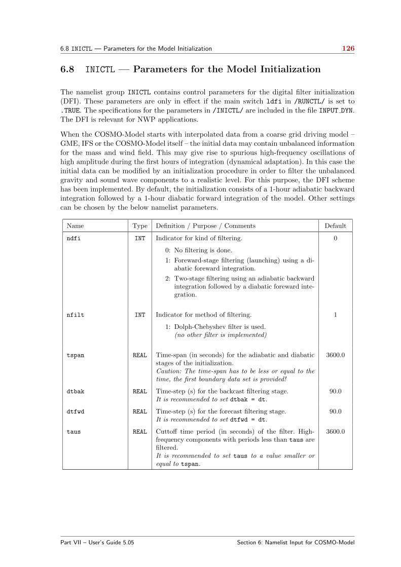
6.8 INICTL — Parameters for the Model Initialization 126
6.8 INICTL — Parameters for the Model Initialization
The namelist group INICTL contains control parameters for the digital filter initialization(DFI). These parameters are only in effect if the main switch ldfi in /RUNCTL/ is set to.TRUE. The specifications for the parameters in /INICTL/ are included in the file INPUT DYN.The DFI is relevant for NWP applications.
When the COSMO-Model starts with interpolated data from a coarse grid driving model –GME, IFS or the COSMO-Model itself – the initial data may contain unbalanced informationfor the mass and wind field. This may give rise to spurious high-frequency oscillations ofhigh amplitude during the first hours of integration (dynamical adaptation). In this case theinitial data can be modified by an initialization procedure in order to filter the unbalancedgravity and sound wave components to a realistic level. For this purpose, the DFI schemehas been implemented. By default, the initialization consists of a 1-hour adiabatic backwardintegration followed by a 1-hour diabatic forward integration of the model. Other settingscan be chosen by the below namelist parameters.
Name Type Definition / Purpose / Comments Default
ndfi INT Indicator for kind of filtering.
0: No filtering is done.
1: Foreward-stage filtering (launching) using a di-abatic foreward integration.
2: Two-stage filtering using an adiabatic backwardintegration followed by a diabatic foreward inte-gration.
0
nfilt INT Indicator for method of filtering.
1: Dolph-Chebyshev filter is used.(no other filter is implemented)
1
tspan REAL Time-span (in seconds) for the adiabatic and diabaticstages of the initialization.Caution: The time-span has to be less or equal to thetime, the first boundary data set is provided!
3600.0
dtbak REAL Time-step (s) for the backcast filtering stage.It is recommended to set dtbak = dt.
90.0
dtfwd REAL Time-step (s) for the forecast filtering stage.It is recommended to set dtfwd = dt.
90.0
taus REAL Cuttoff time period (in seconds) of the filter. High-frequency components with periods less than taus arefiltered.It is recommended to set taus to a value smaller orequal to tspan.
3600.0
Part VII – User’s Guide 5.05 Section 6: Namelist Input for COSMO-Model
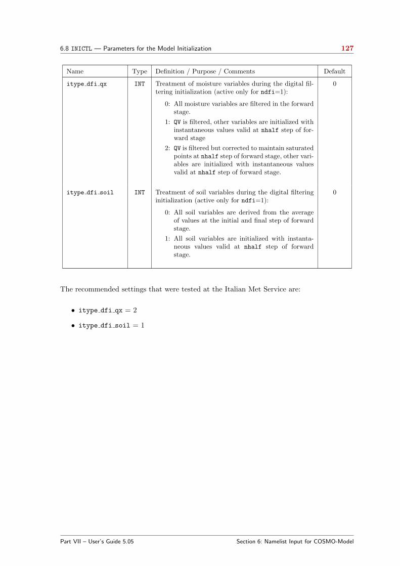
6.8 INICTL — Parameters for the Model Initialization 127
Name Type Definition / Purpose / Comments Default
itype dfi qx INT Treatment of moisture variables during the digital fil-tering initialization (active only for ndfi=1):
0: All moisture variables are filtered in the forwardstage.
1: QV is filtered, other variables are initialized withinstantaneous values valid at nhalf step of for-ward stage
2: QV is filtered but corrected to maintain saturatedpoints at nhalf step of forward stage, other vari-ables are initialized with instantaneous valuesvalid at nhalf step of forward stage.
0
itype dfi soil INT Treatment of soil variables during the digital filteringinitialization (active only for ndfi=1):
0: All soil variables are derived from the averageof values at the initial and final step of forwardstage.
1: All soil variables are initialized with instanta-neous values valid at nhalf step of forwardstage.
0
The recommended settings that were tested at the Italian Met Service are:
• itype dfi qx = 2
• itype dfi soil = 1
Part VII – User’s Guide 5.05 Section 6: Namelist Input for COSMO-Model

6.9 EPSCTL — Controlling the Ensemble Prediction Mode 128
6.9 EPSCTL — Controlling the Ensemble Prediction Mode
The namelist group /EPSCTL/ contains control parameters for the ensemble prediction mode(EPS), e.g. to define the number of members, variations in input- and boundary data andvariations in other namelist parameters to generate ensemble perturbations. The specifica-tions for the parameters in /EPSCTL/ are included in the file INPUT EPS.
Since Version 5.1 there are two more sets of variables in this namelist group, related to thestochastic perturbation of physics tendencies (SPPT) and the generation of random fieldsfor SPPT.
The namelist parameters of this group are described in the subsections
- basic control parameters and
- parameters for changing input fields
- stochastic perturbation of physics tendencies (SPPT)
- generation of random fields for SPPT
Basic control parameters:
Name Type Definition / Purpose / Comments Default
iepsmem INT ID of the member in the ensemble (ID ≥ 0)As a local solution for Grib 1, iepsmem is coded in productdefinition section 52 (ipds(52)).
-1
iepstot INT Total number of ensemble members (≥ 0)As a local solution for Grib 1, iepstot is coded in productdefinition section 51 (ipds(51)).
-1
iepstyp INT ID of the ensemble generation type (ID ≥ 0)As a local solution for Grib 1, iepstyp is coded in productdefinition section 50 (ipds(50)).
-1
Part VII – User’s Guide 5.05 Section 6: Namelist Input for COSMO-Model

6.9 EPSCTL — Controlling the Ensemble Prediction Mode 129
Parameters for changing input fields:
Name Type Definition / Purpose / Comments Default
fac plcov REAL Modification factor for PLCOV 1.0
rmin plcov REAL Lower limit for values of PLCOV 0.0
rmax plcov REAL Upper limit for values of PLCOV 1.0
fac lai REAL Modification factor for LAI 1.0
rmin lai REAL Lower limit for values of LAI 0.0
rmax lai REAL Upper limit for values of LAI 8.0
fac rootdp REAL Modification factor for ROOTDP 1.0
rmin rootdp REAL Lower limit for values of ROOTDP 0.0
rmax rootdp REAL Upper limit for values of ROOTDP 2.0
Parameters for the stochastic perturbation of physics tendencies
The following variables are only in effect, if the namelist variable lsppt in group /RUNCTL/
is set to .TRUE..
Name Type Definition / Purpose / Comments Default
itype qxpert rn INT Defines, which hydrometeor tendencies are perturbed:
0: qv only.
1: qv, qc, qi.
2: qv, qc, qi, qr, qs, qg.
0
itype qxlim rn INT Type of reduction/removal of the perturbation in case ofnegative (for qv, qx) or supersaturated (qv) values
0: No limitation of perturbed tendencies.
1: If new qv values are negative or super-saturatedthen tt T- and tt qv-tendencies are not per-turbed; if new qc, qi, qr, qs, qg-values are neg-ative then the corresponding tendencies are not per-turbed.
0
ltargetdiff mask LOG To switch off SPPT locally if targeted diffusion is active.(introduced in Version 5.04g)
.FALSE.
Part VII – User’s Guide 5.05 Section 6: Namelist Input for COSMO-Model
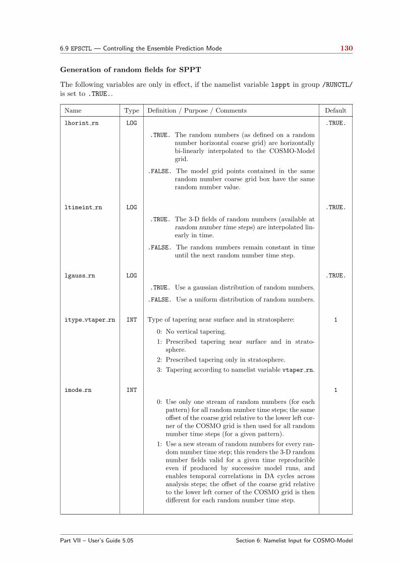
6.9 EPSCTL — Controlling the Ensemble Prediction Mode 130
Generation of random fields for SPPT
The following variables are only in effect, if the namelist variable lsppt in group /RUNCTL/
is set to .TRUE..
Name Type Definition / Purpose / Comments Default
lhorint rn LOG
.TRUE. The random numbers (as defined on a randomnumber horizontal coarse grid) are horizontallybi-linearly interpolated to the COSMO-Modelgrid.
.FALSE. The model grid points contained in the samerandom number coarse grid box have the samerandom number value.
.TRUE.
ltimeint rn LOG
.TRUE. The 3-D fields of random numbers (available atrandom number time steps) are interpolated lin-early in time.
.FALSE. The random numbers remain constant in timeuntil the next random number time step.
.TRUE.
lgauss rn LOG
.TRUE. Use a gaussian distribution of random numbers.
.FALSE. Use a uniform distribution of random numbers.
.TRUE.
itype vtaper rn INT Type of tapering near surface and in stratosphere:
0: No vertical tapering.
1: Prescribed tapering near surface and in strato-sphere.
2: Prescribed tapering only in stratosphere.
3: Tapering according to namelist variable vtaper rn.
1
imode rn INT
0: Use only one stream of random numbers (for eachpattern) for all random number time steps; the sameoffset of the coarse grid relative to the lower left cor-ner of the COSMO grid is then used for all randomnumber time steps (for a given pattern).
1: Use a new stream of random numbers for every ran-dom number time step; this renders the 3-D randomnumber fields valid for a given time reproducibleeven if produced by successive model runs, andenables temporal correlations in DA cycles acrossanalysis steps; the offset of the coarse grid relativeto the lower left corner of the COSMO grid is thendifferent for each random number time step.
1
Part VII – User’s Guide 5.05 Section 6: Namelist Input for COSMO-Model
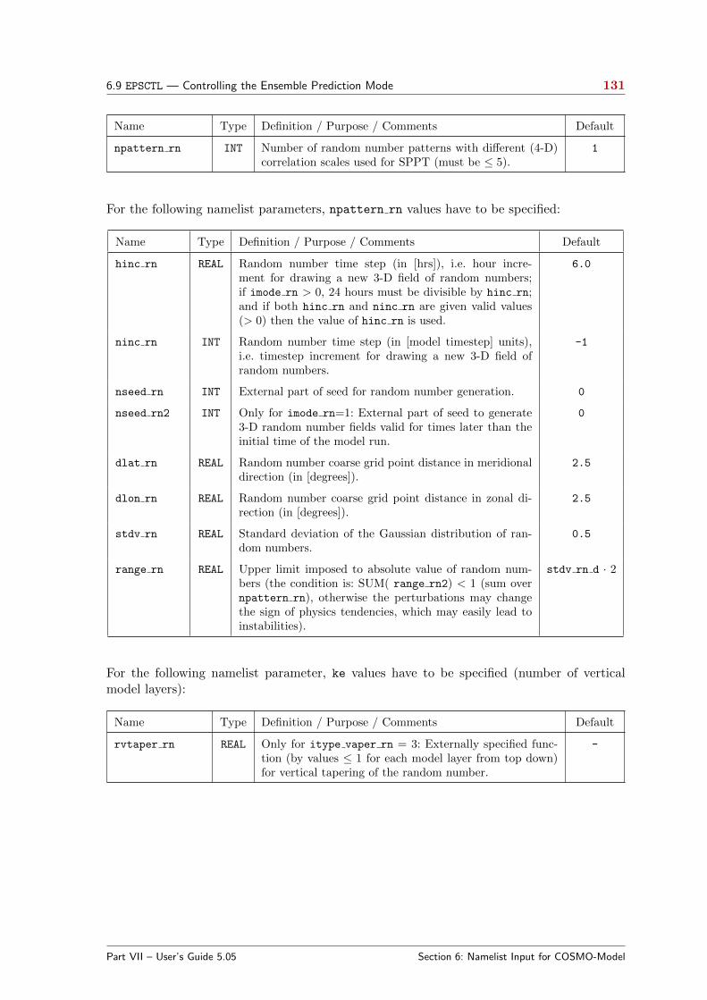
6.9 EPSCTL — Controlling the Ensemble Prediction Mode 131
Name Type Definition / Purpose / Comments Default
npattern rn INT Number of random number patterns with different (4-D)correlation scales used for SPPT (must be ≤ 5).
1
For the following namelist parameters, npattern rn values have to be specified:
Name Type Definition / Purpose / Comments Default
hinc rn REAL Random number time step (in [hrs]), i.e. hour incre-ment for drawing a new 3-D field of random numbers;if imode rn > 0, 24 hours must be divisible by hinc rn;and if both hinc rn and ninc rn are given valid values(> 0) then the value of hinc rn is used.
6.0
ninc rn INT Random number time step (in [model timestep] units),i.e. timestep increment for drawing a new 3-D field ofrandom numbers.
-1
nseed rn INT External part of seed for random number generation. 0
nseed rn2 INT Only for imode rn=1: External part of seed to generate3-D random number fields valid for times later than theinitial time of the model run.
0
dlat rn REAL Random number coarse grid point distance in meridionaldirection (in [degrees]).
2.5
dlon rn REAL Random number coarse grid point distance in zonal di-rection (in [degrees]).
2.5
stdv rn REAL Standard deviation of the Gaussian distribution of ran-dom numbers.
0.5
range rn REAL Upper limit imposed to absolute value of random num-bers (the condition is: SUM( range rn2) < 1 (sum overnpattern rn), otherwise the perturbations may changethe sign of physics tendencies, which may easily lead toinstabilities).
stdv rn d · 2
For the following namelist parameter, ke values have to be specified (number of verticalmodel layers):
Name Type Definition / Purpose / Comments Default
rvtaper rn REAL Only for itype vaper rn = 3: Externally specified func-tion (by values ≤ 1 for each model layer from top down)for vertical tapering of the random number.
-
Part VII – User’s Guide 5.05 Section 6: Namelist Input for COSMO-Model
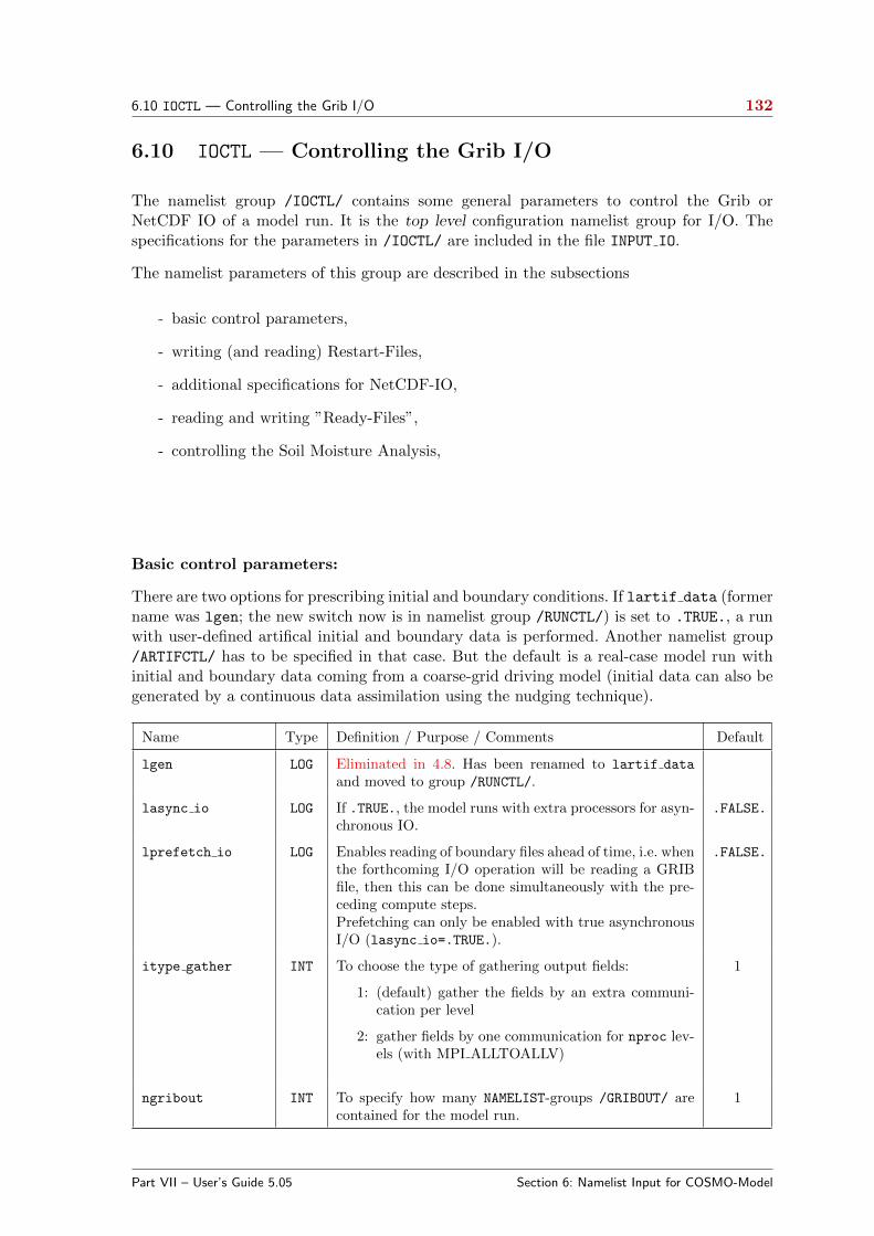
6.10 IOCTL — Controlling the Grib I/O 132
6.10 IOCTL — Controlling the Grib I/O
The namelist group /IOCTL/ contains some general parameters to control the Grib orNetCDF IO of a model run. It is the top level configuration namelist group for I/O. Thespecifications for the parameters in /IOCTL/ are included in the file INPUT IO.
The namelist parameters of this group are described in the subsections
- basic control parameters,
- writing (and reading) Restart-Files,
- additional specifications for NetCDF-IO,
- reading and writing ”Ready-Files”,
- controlling the Soil Moisture Analysis,
Basic control parameters:
There are two options for prescribing initial and boundary conditions. If lartif data (formername was lgen; the new switch now is in namelist group /RUNCTL/) is set to .TRUE., a runwith user-defined artifical initial and boundary data is performed. Another namelist group/ARTIFCTL/ has to be specified in that case. But the default is a real-case model run withinitial and boundary data coming from a coarse-grid driving model (initial data can also begenerated by a continuous data assimilation using the nudging technique).
Name Type Definition / Purpose / Comments Default
lgen LOG Eliminated in 4.8. Has been renamed to lartif data
and moved to group /RUNCTL/.
lasync io LOG If .TRUE., the model runs with extra processors for asyn-chronous IO.
.FALSE.
lprefetch io LOG Enables reading of boundary files ahead of time, i.e. whenthe forthcoming I/O operation will be reading a GRIBfile, then this can be done simultaneously with the pre-ceding compute steps.Prefetching can only be enabled with true asynchronousI/O (lasync io=.TRUE.).
.FALSE.
itype gather INT To choose the type of gathering output fields:
1: (default) gather the fields by an extra communi-cation per level
2: gather fields by one communication for nproc lev-els (with MPI ALLTOALLV)
1
ngribout INT To specify how many NAMELIST-groups /GRIBOUT/ arecontained for the model run.
1
Part VII – User’s Guide 5.05 Section 6: Namelist Input for COSMO-Model
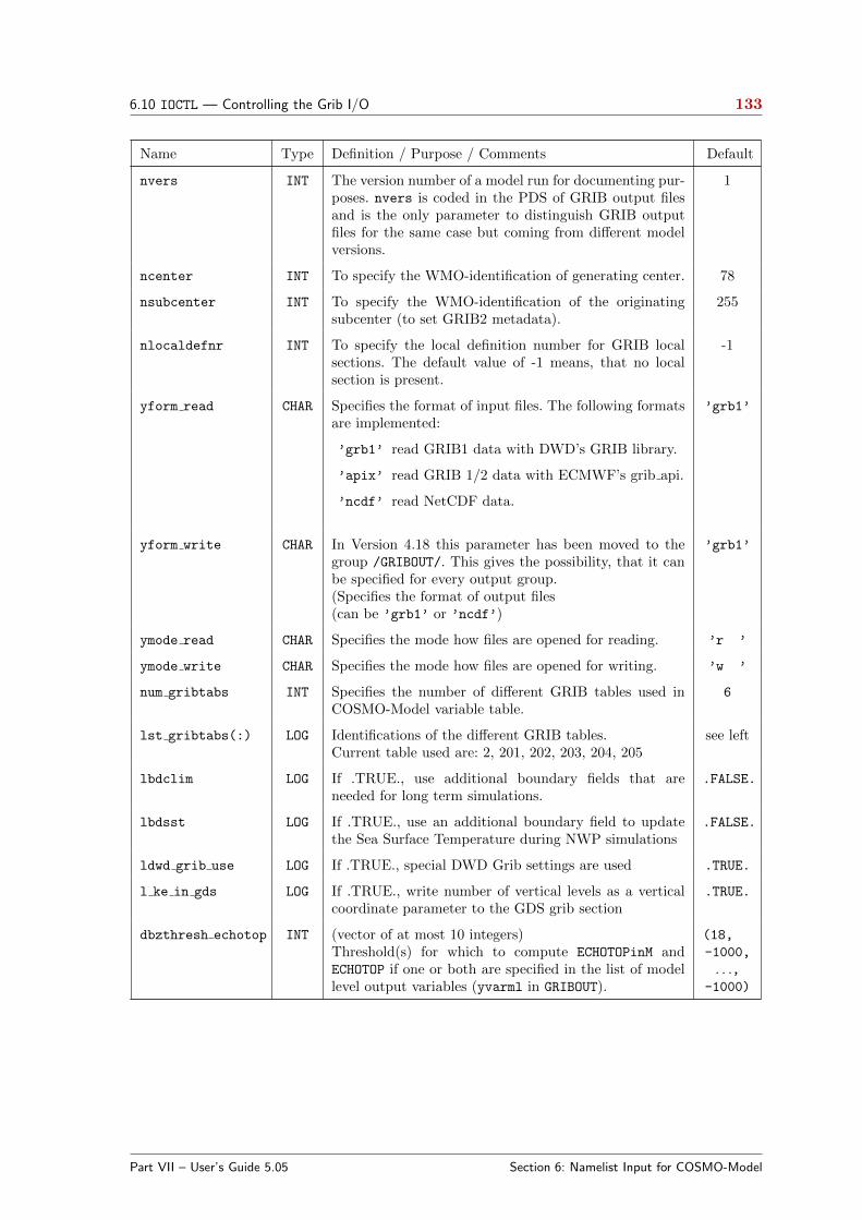
6.10 IOCTL — Controlling the Grib I/O 133
Name Type Definition / Purpose / Comments Default
nvers INT The version number of a model run for documenting pur-poses. nvers is coded in the PDS of GRIB output filesand is the only parameter to distinguish GRIB outputfiles for the same case but coming from different modelversions.
1
ncenter INT To specify the WMO-identification of generating center. 78
nsubcenter INT To specify the WMO-identification of the originatingsubcenter (to set GRIB2 metadata).
255
nlocaldefnr INT To specify the local definition number for GRIB localsections. The default value of -1 means, that no localsection is present.
-1
yform read CHAR Specifies the format of input files. The following formatsare implemented:
’grb1’ read GRIB1 data with DWD’s GRIB library.
’apix’ read GRIB 1/2 data with ECMWF’s grib api.
’ncdf’ read NetCDF data.
’grb1’
yform write CHAR In Version 4.18 this parameter has been moved to thegroup /GRIBOUT/. This gives the possibility, that it canbe specified for every output group.(Specifies the format of output files(can be ’grb1’ or ’ncdf’)
’grb1’
ymode read CHAR Specifies the mode how files are opened for reading. ’r ’
ymode write CHAR Specifies the mode how files are opened for writing. ’w ’
num gribtabs INT Specifies the number of different GRIB tables used inCOSMO-Model variable table.
6
lst gribtabs(:) LOG Identifications of the different GRIB tables.Current table used are: 2, 201, 202, 203, 204, 205
see left
lbdclim LOG If .TRUE., use additional boundary fields that areneeded for long term simulations.
.FALSE.
lbdsst LOG If .TRUE., use an additional boundary field to updatethe Sea Surface Temperature during NWP simulations
.FALSE.
ldwd grib use LOG If .TRUE., special DWD Grib settings are used .TRUE.
l ke in gds LOG If .TRUE., write number of vertical levels as a verticalcoordinate parameter to the GDS grib section
.TRUE.
dbzthresh echotop INT (vector of at most 10 integers)Threshold(s) for which to compute ECHOTOPinM andECHOTOP if one or both are specified in the list of modellevel output variables (yvarml in GRIBOUT).
(18,
-1000,
. . .,-1000)
Part VII – User’s Guide 5.05 Section 6: Namelist Input for COSMO-Model
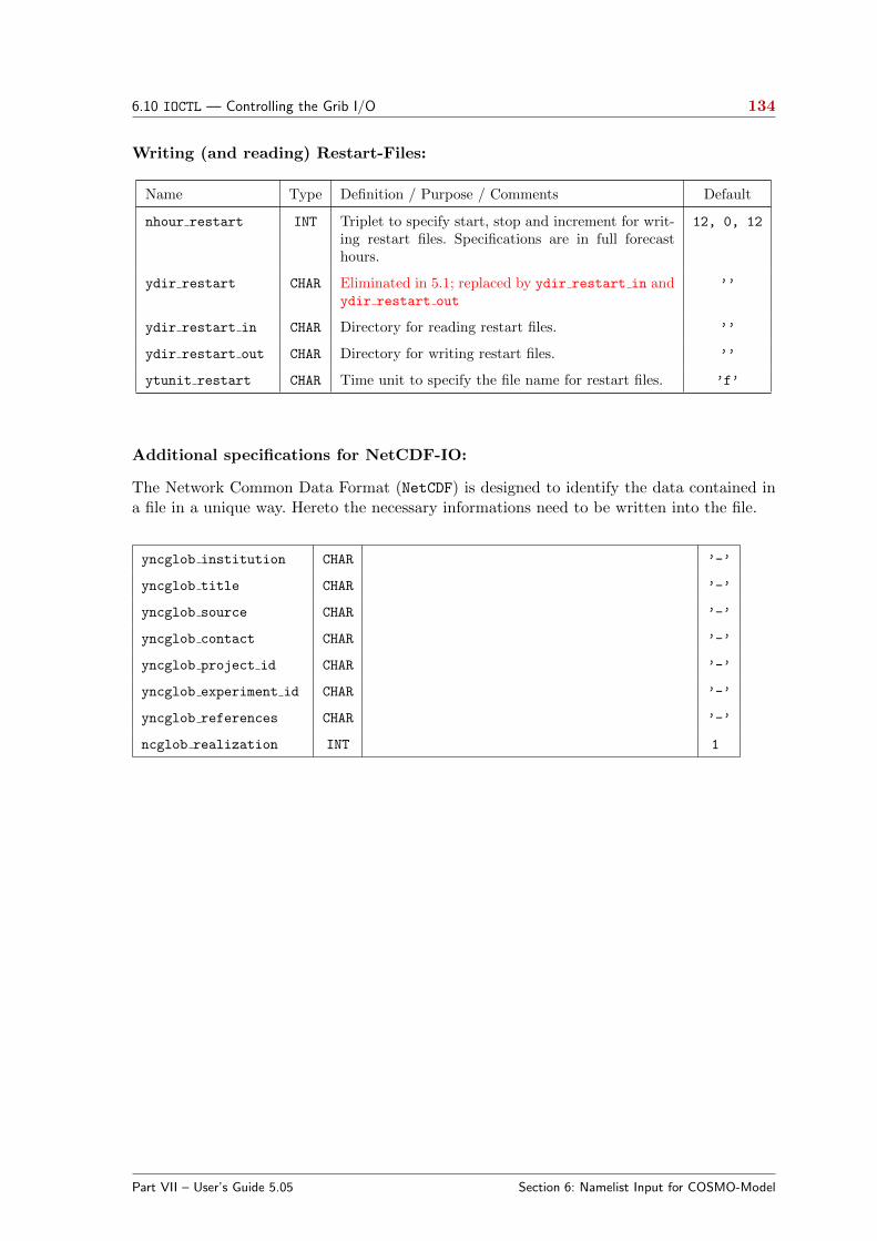
6.10 IOCTL — Controlling the Grib I/O 134
Writing (and reading) Restart-Files:
Name Type Definition / Purpose / Comments Default
nhour restart INT Triplet to specify start, stop and increment for writ-ing restart files. Specifications are in full forecasthours.
12, 0, 12
ydir restart CHAR Eliminated in 5.1; replaced by ydir restart in andydir restart out
’’
ydir restart in CHAR Directory for reading restart files. ’’
ydir restart out CHAR Directory for writing restart files. ’’
ytunit restart CHAR Time unit to specify the file name for restart files. ’f’
Additional specifications for NetCDF-IO:
The Network Common Data Format (NetCDF) is designed to identify the data contained ina file in a unique way. Hereto the necessary informations need to be written into the file.
yncglob institution CHAR ’-’
yncglob title CHAR ’-’
yncglob source CHAR ’-’
yncglob contact CHAR ’-’
yncglob project id CHAR ’-’
yncglob experiment id CHAR ’-’
yncglob references CHAR ’-’
ncglob realization INT 1
Part VII – User’s Guide 5.05 Section 6: Namelist Input for COSMO-Model

6.10 IOCTL — Controlling the Grib I/O 135
Reading and writing “Ready-Files”:
In an operational environment, the COSMO-Model can also be run in parallel with the in-terpolation program which generates lateral boundary conditions from the correspondingcoarse-grid model run. In this case, the interpolation program writes so-called ready-files,which simply indicate that a lateral boundary file for a certain forecast time has been success-fully and completely written. During program execution, the model checks for the existence ofthese files in certain time intervals – and in this way waits until the required lateral boundarydata-set is available for the next READ-operation on the corresponding input file. In a simi-lar way, the COSMO-Model writes ready files for each output file that has been successfullywritten. This allows to run postprocessing utilities in parallel to the model execution.
ytrans in CHAR Directory path for reading ready-files. ’ ’
ytrans out CHAR Directory path for writing ready-files. ’ ’
nincwait INT Seconds to wait until the next read attempt for a lateral bound-ary file if the corresponding ready file is not available.
0
nmaxwait INT Maximum seconds to wait until abort if the ready file for thenext lateral boundary file is not available.
0
Controlling the Soil Moisture Analysis:
nsma stat INT Status for soil moisture analysis. nsma stat is coded in thePDS of the grib-ed fields for soil moisture content (in the “localuse area”).
0: this is a “normal” soil moisture field.
20: this is a field derived by soil moisture analysis.
0
Part VII – User’s Guide 5.05 Section 6: Namelist Input for COSMO-Model

6.11 DATABASE — Specification of Database Job 136
6.11 DATABASE — Specification of Database Job
This Namelist group has been eliminated in Version 4.25, since the direct writing to thedatabase system has never been used!
Instead of using the file-based GRIB-IO, there is also a capability to read and write GRIB-files directly from a database system. However, this option works only if you work within theDWD IT-environment, which provides a very special but not portable interface csodaban
to a commercial database system. To use this option, you should be familiar with the DWDdatabase interface and the structure of the database system.
All users outside DWD have to work with file-based IO. Most Namelist input parametersfrom DATABASE are not relevant in this case – except nout sockets and nin sockets whichboth have to be set to 0 (default) in order to enable file-based IO.
Name Type Definition / Purpose / Comments Default
yinit order CHAR String to initialize the data-base interface program csodaban
for GRIB-IO, including specifications to write GRIB outputto the data base system.
’ak=nix’
yana tab CHAR Specifications to retrieve initial data from the data basesystem.
’*****’
ybd tab CHAR Specifications to retrieve boundary data from the data basesystem.
’*****’
nout sockets INT Number of sockets for database output per PE(0 means File-IO).
0
nin sockets INT Number of sockets for database input per PE(0 means File-IO; has to be ≤ 1).
0
iretry INT Number of seconds to retry on database failure. 0
ibackup size INT Size of incore backup space (in bytes) by a database failure. -1
ybackup dir CHAR Directory path for outcore backup. ’.’
idbg level INT Debug level for mpe io. 0
Part VII – User’s Guide 5.05 Section 6: Namelist Input for COSMO-Model

6.12 GRIBIN — Controlling the Grib Input 137
6.12 GRIBIN — Controlling the Grib Input
The namelist group /GRIBIN/ contains parameters related to the input of initial and bound-ary files, which are an analysis file for the initialization of the model fields (containing alsothe constant parameter fields such as orography, soil type etc.), and boundary data files forcertain equidistant boundary update time steps.
Note that the namelist group /GRIBIN/ applies to all possible input data formats (GRIB,NetCDF), not only to GRIB data. The specifications for the parameters in /GRIBIN/ areincluded in the file INPUT IO.
Each namelist parameters of the list is described in one of the sections:
- control parameters for initial data,
- control parameters for boundary data and
- additional parameters for continuous data assimilation
Control parameters for initial data
Name Type Definition / Purpose / Comments Default
ydirini CHAR Directory path of the initial data file – interpolated datafrom a driving model or analysis from a continuous COSMO-Model data assimilation.
’ ’
lchkini LOG Checking the initial data for min/max values. .FALSE.
yvarini(:) CHAR has been eliminated in Version 4.12.
lana qi LOG If .TRUE., use the cloud-ice field contained in the initialdata file as initial condition for cloud-ice; otherwise, initialconditions for cloud-ice are set in the model.
.FALSE.
lana qr qs LOG If .TRUE., values for rain and snow are read from the initialconditions. Otherwise, values are set in the model.
.FALSE.
lana qg LOG If .TRUE., values for the graupel scheme are provided in theinitial data;
.FALSE.
lana rho snow LOG If .TRUE., values for the density of snow are provided inthe initial data;
.FALSE.
nlgw ini INT Eliminated in Version 5.05Number of prognostic soil water levels in initial data. Thisparameter is only used for the “old” soil model.
2
nsec fg INT Lead time (in [s], as integer) of first guess file for incrementalanalysis update.(Introduced in Version 5.04d).
3600
Part VII – User’s Guide 5.05 Section 6: Namelist Input for COSMO-Model

6.12 GRIBIN — Controlling the Grib Input 138
Control parameters for boundary data
Name Type Definition / Purpose / Comments Default
hincbound REAL Interval in hours between two consecutive sets of bound-ary data (boundary update frequency). Within this timeinterval, boundary values are interpolated linearly intime. Only multiples of 0.25 are possible.
1.0
ydirbd CHAR Directory path of the boundary data files. ’ ’
lchkbd LOG Checking the boundary data for min/max values. .FALSE.
yvarbd CHAR has been eliminated in Version 4.12.
llb qi LOG If .TRUE., take cloud-ice values contained in the lat-eral boundary data as boundary condition for cloud ice;otherwise, cloud ice boundary conditions are set in themodel.
.FALSE.
llb qr qs LOG If .TRUE., take rain and snow values contained in thelateral boundary data as boundary condition.
.FALSE.
llb qg LOG If .TRUE., take graupel values contained in the lateralboundary data as boundary condition.
.FALSE.
lbdana LOG If .TRUE., use analysis data as lateral boundary condi-tions.
.FALSE.
lic2bc LOG If .TRUE., use initial conditions as boundary data attimestep 0.(Introduced in Version 5.04d).
.FALSE.
sic2bc REAL Period (in [s]) in which the initial conditions are addi-tionally used for the lateral boundary conditions (withweight 1 at time 0 decreasing linearly to zero at timesic2bc)(Introduced in Version 5.04d).
3600.0
hlastbc REAL Boundary fields valid later than this lead time [hour] arenot read (boundary conditions beyond that time limitare obtained by linear extrapolation of boundary fields).(Introduced in Version 5.04d).
hstop+100
ytunitbd CHAR Time unit indicator in the boundary data file name (seeSection 6.2).
t forecast range given in timesteps
f the forecast range is given in the form ddhhmmss
(where dd: day, hh: hour, mm: minute, ss: second)
c the forecast range is given in the form yyydddhh
(yyy: year, ddd: day of the year, hh: hour)
d the forecast range is given in the form yyyymmddhh
or (optionally) yyyymmddhhmise (can only beused, if hincbound is given in full hours) (Use ’d’for COSMO-CLM)
’f’
nlgw bd INT Eliminated in Version 5.05Number of prognostic soil water levels in boundary data.This parameter is only used for the “old” soil model.
2
Part VII – User’s Guide 5.05 Section 6: Namelist Input for COSMO-Model
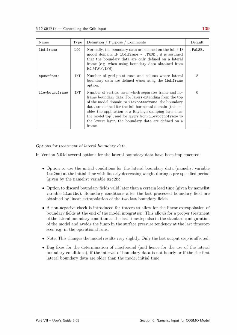
6.12 GRIBIN — Controlling the Grib Input 139
Name Type Definition / Purpose / Comments Default
lbd frame LOG Normally, the boundary data are defined on the full 3-Dmodel domain. IF lbd frame = .TRUE., it is assumedthat the boundary data are only defined on a lateralframe (e.g. when using boundary data obtained fromECMWF/IFS).
.FALSE.
npstrframe INT Number of grid-point rows and colums where lateralboundary data are defined when using the lbd frame
option.
8
ilevbotnoframe INT Number of vertical layer which separates frame and no-frame boundary data. For layers extending from the topof the model domain to ilevbotnoframe, the boundarydata are defined for the full horizontal domain (this en-ables the application of a Rayleigh damping layer nearthe model top), and for layers from ilevbotnoframe tothe lowest layer, the boundary data are defined on aframe.
0
Options for treatment of lateral boundary data
In Version 5.04d several options for the lateral boundary data have been implemented:
• Option to use the initial conditions for the lateral boundary data (namelist variablelic2bc) at the initial time with linearly decreasing weight during a pre-specified period(given by the namelist variable sic2bc.
• Option to discard boundary fields valid later than a certain lead time (given by namelistvariable hlastbc). Boundary conditions after the last processed boundary field areobtained by linear extrapolation of the two last boundary fields.
• A non-negative check is introduced for tracers to allow for the linear extrapolation ofboundary fields at the end of the model integration. This allows for a proper treatmentof the lateral boundary condition at the last timestep also in the standard configurationof the model and avoids the jump in the surface pressure tendency at the last timestepseen e.g. in the operational runs.
• Note: This changes the model results very slightly. Only the last output step is affected.
• Bug fixes for the determination of nlastbound (and hence for the use of the lateralboundary conditions), if the interval of boundary data is not hourly or if the the firstlateral boundary data are older than the model initial time.
Part VII – User’s Guide 5.05 Section 6: Namelist Input for COSMO-Model

6.12 GRIBIN — Controlling the Grib Input 140
Additional parameters for continuous data assimilation
Name Type Definition / Purpose / Comments Default
newbc INT Number of times that boundary update is analysis after 1hour.
360
newbcdt INT Time step increment of boundary update from analysis. ’ ’
hnewbcdt REAL Hour increment of boundary update from analysis. 0.0
nincboufac INT Factor to nincbound when new boundary update is analysis. 2
lan t s LOG Selection of analysed (tri=0) sea surface temperature. .FALSE.
lan t so0 LOG Selection of analysed (tri=0) sea surface temperature (for themulti-layer soil model.
.FALSE.
lan t snow LOG Selection of analysed snow temperature. .FALSE.
lan t cl LOG Selection of analysed climatological soil temperature. .FALSE.
lan w snow LOG Selection of analysed water content of snow. .FALSE.
lan w i LOG Selection of analysed interception water. .FALSE.
lan w so LOG Selection of analysed or external soil moisture. .FALSE.
lan w cl LOG Selection of analysed climatological soil water content. .FALSE.
lan vio3 LOG Selection of analysed vertical integrated ozone. .FALSE.
lan hmo3 LOG Selection of analysed ozone maximum. .FALSE.
lan plcov LOG Selection of analysed plant cover. .FALSE.
lan lai LOG Selection of analysed leaf area index. .FALSE.
lan rootdp LOG Selection of analysed root depth. .FALSE.
lan rho snow LOG Selection of analysed density of snow. .FALSE.
The control of the parameters lan xxx is as follows:.TRUE.: Fields are used from external analyses or from an interpolated coarse grid field..FALSE.: Fields are used from the continous data assimilation of the COSMO-Model.
Part VII – User’s Guide 5.05 Section 6: Namelist Input for COSMO-Model

6.13 GRIBOUT — Controlling the Grib Output 141
6.13 GRIBOUT — Controlling the Grib Output
How to use the NAMELIST group GRIBOUT is explained in more detail in Part VI of theCOSMO-Model Documentation: Model Output and Data Formats for I/O.
Basic parameters for controlling the output:
Name Type Definition / Purpose / Comments Default
ydir CHAR Directory of the output file. ’ ’
yvarml(:) CHAR List of model variables for output
yvarpl(:) CHAR List of variables for pressure levels
plev(:) REAL Pressure levels
yvarzl(:) CHAR List of variables for z-levels
zlev(:) REAL Z-levels
yvarsl(:) CHAR List of satellite channels for output
ngrib(:) INT List of output steps given in time steps 99999
ncomb(:) INT Triplets for building ngrib 99999
hgrib(:) REAL List of output steps given in hours 0.0
hcomb(:) REAL Triplets for building ngrib 0.0
Controlling the output domain and time unit indicator:
ytunit CHAR Time unit indicator in the output data file name (see Sec-tion 6.2).
’f’
ydomain CHAR Domain type (full or sub) indicator in the output data filename (see Section 6.2).
’f’
slon REAL Left longitude for a subdomain startlon tot
slat REAL Bottom latitude for a subdomain startlat tot
elon REAL Right longitude for a subdomain endlon tot
elat REAL Upper latitude for a subdomain endlat tot
Part VII – User’s Guide 5.05 Section 6: Namelist Input for COSMO-Model
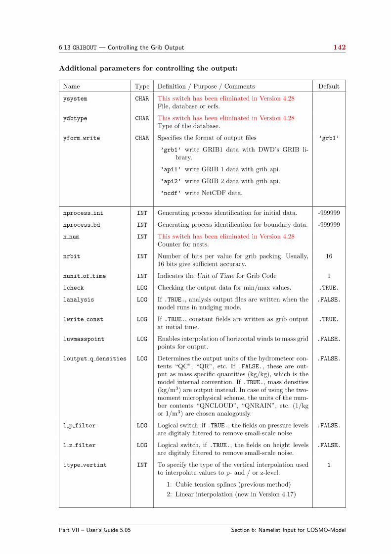
6.13 GRIBOUT — Controlling the Grib Output 142
Additional parameters for controlling the output:
Name Type Definition / Purpose / Comments Default
ysystem CHAR This switch has been eliminated in Version 4.28File, database or ecfs.
ydbtype CHAR This switch has been eliminated in Version 4.28Type of the database.
yform write CHAR Specifies the format of output files
’grb1’ write GRIB1 data with DWD’s GRIB li-brary.
’api1’ write GRIB 1 data with grib api.
’api2’ write GRIB 2 data with grib api.
’ncdf’ write NetCDF data.
’grb1’
nprocess ini INT Generating process identification for initial data. -999999
nprocess bd INT Generating process identification for boundary data. -999999
n num INT This switch has been eliminated in Version 4.28Counter for nests.
nrbit INT Number of bits per value for grib packing. Usually,16 bits give sufficient accuracy.
16
nunit of time INT Indicates the Unit of Time for Grib Code 1
lcheck LOG Checking the output data for min/max values. .TRUE.
lanalysis LOG If .TRUE., analysis output files are written when themodel runs in nudging mode.
.FALSE.
lwrite const LOG If .TRUE., constant fields are written as grib outputat initial time.
.TRUE.
luvmasspoint LOG Enables interpolation of horizontal winds to mass gridpoints for output.
.FALSE.
loutput q densities LOG Determines the output units of the hydrometeor con-tents “QC”, “QR”, etc. If .FALSE., these are out-put as mass specific quantities (kg/kg), which is themodel internal convention. If .TRUE., mass densities(kg/m3) are output instead. In case of using the two-moment microphysical scheme, the units of the num-ber contents “QNCLOUD”, “QNRAIN”, etc. (1/kgor 1/m3) are chosen analogously.
.FALSE.
l p filter LOG Logical switch, if .TRUE., the fields on pressure levelsare digitaly filtered to remove small-scale noise
.FALSE.
l z filter LOG Logical switch, if .TRUE., the fields on height levelsare digitaly filtered to remove small-scale noise.
.FALSE.
itype vertint INT To specify the type of the vertical interpolation usedto interpolate values to p- and / or z-level.
1: Cubic tension splines (previous method)
2: Linear interpolation (new in Version 4.17)
1
Part VII – User’s Guide 5.05 Section 6: Namelist Input for COSMO-Model

6.13 GRIBOUT — Controlling the Grib Output 143
Name Type Definition / Purpose / Comments Default
l fi ps smooth LOG This switch has been renamed (see below), becausewhat really is smoothed here is the mean sea levelpressure!
---
l fi pmsl smooth LOG Logical switch, if .TRUE., additional smoothing isdone for mean sea-level pressure and geopotential inmountainous areas.
.FALSE.
l fi filter LOG Logical switch to filter the geopotential FI indepen-dent of the settings of l p filter.
.FALSE.
l pmsl filter LOG Logical switch to filter the mean sea level pressurePMSL independent of the settings of l p filter and/ or l z filter
.TRUE.
ysuffix CHAR To add an optional suffix to the file names. ’’
Part VII – User’s Guide 5.05 Section 6: Namelist Input for COSMO-Model

6.13 GRIBOUT — Controlling the Grib Output 144
Handling of statistically processed fields:
The new diagnostic output variables for tracking of convective cells need a modified treatmentof statistically processed fields, because they should be reset after every output step.
Up to now only the following methods are possible in the COSMO-Model: Statistical pro-cessing by
• summation or averaging:Fields are summed up from beginning of the simulation and never reset. Only in climatemode (lbdclim=.TRUE.) the fields are reset to 0.0 after an output step.
• Min / Max values:
– Temperatures (TMIN 2M, TMAX 2M) are reset according to the namelist variablehincmxt in /RUNCTL/.
– Wind speeds and gusts (e.g. VMAX 10M, VABS 10M, VGUST DYN 10M, VGUST CON 10M)are reset according to namelist variable hincmxu in /RUNCTL/.
– the new MAX-variables for tracking of convective cells should be reset after everyoutput. The difficulty here is, that these variables could occur in different GRIBOUTnamelist groups.
A more generalized way has been implemented in the COSMO-Model, Version 5.05, how theresetting of statistically processed fields is organized.
All statistically processed fields are grouped into four categories.
Temperatures TMIN 2M, TMAX 2M,
Winds VMAX 10M, VABSMX 10M, VGUST DYN 10M, VGUST CON 10M,
Summations / T 2M AV, TD 2M AV, U 10M AV, V 10M AV,
Averages ASOB S, ATHB S, ASOB T, ATHB T,
ALHFL S, ASHFL S, AUMFL S, AVMFL S,
APAB S, ALHFL BS, ALHFL PL, ASWDIR S,
ASWDIFD S, ASWDIFU S, ATHD S, ATHU S,
ASOD T, AUSTR SSO, AVSTR SSO, AVDIS SSO,
AEVAP S, TOT PREC, SNOW CON, SNOW GSP,
RUNOFF S, RUNOFF G, SNOW MELT, DURSUN,
TDIV HUM, RAIN GSP, RAIN CON, GRAU GSP,
HAIL GSP, DURSUN M, DURSUN R,
Cells TCOND MAX, TCOND10 MX, LPI MAX, DBZ CTMAX,
UH MAX, VORW CTMAX, W CTMAX,
Part VII – User’s Guide 5.05 Section 6: Namelist Input for COSMO-Model
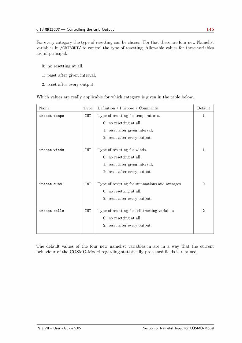
6.13 GRIBOUT — Controlling the Grib Output 145
For every category the type of resetting can be chosen. For that there are four new Namelistvariables in /GRIBOUT/ to control the type of resetting. Allowable values for these variablesare in principal:
0: no resetting at all,
1: reset after given interval,
2: reset after every output.
Which values are really applicable for which category is given in the table below.
Name Type Definition / Purpose / Comments Default
ireset temps INT Type of resetting for temperatures.
0: no resetting at all,
1: reset after given interval,
2: reset after every output.
1
ireset winds INT Type of resetting for winds.
0: no resetting at all,
1: reset after given interval,
2: reset after every output.
1
ireset sums INT Type of resetting for summations and averages
0: no resetting at all,
2: reset after every output.
0
ireset cells INT Type of resetting for cell tracking variables
0: no resetting at all,
2: reset after every output.
2
The default values of the four new namelist variables in are in a way that the currentbehaviour of the COSMO-Model regarding statistically processed fields is retained.
Part VII – User’s Guide 5.05 Section 6: Namelist Input for COSMO-Model

146
Section 7
Namelist Input for DataAssimilation
7.1 NUDGING — Controlling the Data Assimilation
The NAMELIST group ’/NUDGING/’ is required and read only if the compile option ’-DNUDGING’is used for the production of the COSMO binary and if the namelist parameter luseobs in/RUNCTL/ is set to .TRUE..
/NUDGING/ contains the variables that control all the processes which require meteorologicalobservations, except for the use of satellite radiances in order to produce synthethic satelliteimages (see NAMELIST group ’/SATCTL/’). Figure 7.1 shows an example for it as an excerptof the script that is used to run the COSMO-Model.
Note that the whole of the namelist group ’/NUDGING/’ has no effect at all as long as theNAMELIST variable ’luseobs’ of NAMELIST group ’/RUNCTL/’ is set to .FALSE.. This meansthat if a free model forecast is to be performed solely, it is sufficient to set luseobs=.FALSE.,and the group ’/NUDGING/’ does not have to be concerned with.
At present, there a four main processes requiring observations:
− data assimilation based on the nudging technique for atmospheric variables
− verification, which means here simply the writing of a NetCDF feedobs file and / or averification observation file VOF for the purpose of observation input for the LETKFanalysis scheme or input for verification tools (see Part VI: Model Output and DataFormats for I/O for more information on feedobs files and verification observation files).
− latent heat nudging (LHN) for the assimilation of radar-derived surface precipitationrates
− production of 2-dimensional (2D) surface-level analyses based on (synoptic) observa-tions; these analyses can be used for validation purposes or as input for the variationalsoil moisture analysis (SMA).
Part VII – User’s Guide 5.05 Section 7: Namelist Input for Data Assimilation

7.1 NUDGING — Controlling the Data Assimilation 147
cat > INPUT_ASS << end_input_ass
&NUDGING
lnudge =.TRUE.,
hnudgsta= 0.0, hnudgend = 7.0, tconbox = 180.0,
lverif =.TRUE., lverpas = .TRUE., nveripr = 3,
llhn =.TRUE., llhnverif=.TRUE., lhn_wweight=.TRUE., rqrsgmax= 0.4,
radar_in=’./’,
ycdfdir =’./’,
hversta = 0.001, hverend = 3.0,
nwtyp = 7,
niwtyp = 1,4,2,1,1,3,1
iwtyp = 0,-132,-133,-136,-137,1,4,2,9,-823,-830,-930,12,
kwtyp = 1,1,1,1,2,2,2,2,1,
khumbal = 100,
mruntyp = 2,
ntpscor = 1, ptpstop=400.0, luvgcor=.TRUE., mpsgcor = 1,
ltipol =.TRUE., tipolmx = 3.0, wtukrsa = 3.0, wtukrse = 1.0,
ltipsu =.TRUE., tipmxsu = 1.0, wtuksua = 1.5, wtuksue = 0.5,
wtukara = 1.5, wtukare = 0.5,
msprpar = 1, msprpsu = 0,
gnudg = 0.0006, 0.0012, 0.0006, 0.0006,
gnudgsu = 0.0006, 0.0012, 0.0000, 0.0006,
gnudgar = .0006, .0000, .0006, .0000,
gnudggp = 0.0003,
vcorls = .333 , .333 , .04 , .04 , vcutof = 0.75, 0.75, 1.0 , 1.0 ,
vcorlsu = .013 , .013 , .002 ,.00001, vcutosu = 0.75, 0.75, 4.0 ,0.001,
vcsnisu = 2500., 2500., 9. , 9. ,
rhvfac = 1.0 , 0.0 , 0.83, 0.83,
rhinfl = 0., 70., 0., 0., rhtfac = 1.3 , 1.43, 1.3 , 1.3 ,
rhiflsu = 70., 70., 100., 70., rhtfsu = 1.0 , 1.43, 1.0 , 1.0 ,
fnondiv = 0.8 , cnondiv = 0.1 , cutofr = 3.5 , 3.5 , 3.5 , 3.5 ,
tnondiv = 1.1 , cutofsu = 2.0 , 3.5 , 2.0 , 2.0 ,
topobs = 849., 1099., 799., 699.,
botmod = 1099., 1099., 1099., 899.,
lscadj =.TRUE.,.TRUE.,.TRUE.,.FALSE.,
dtqc = 720., qcvf = 5.00, 1.00,10.00, 1.00,
qcc = 0.00,500.00, 0.00, 0.00,
qccsu = 12., 500., 12., .7,
mqcorr92= 0,
lsynop =.TRUE., laircf =.TRUE., ldribu =.TRUE., ltemp =.TRUE.,
lpilot =.TRUE., lsatem =.FALSE., lgps =.TRUE.,
lscatt =.TRUE., lcd122 =.TRUE., lcd123 =.TRUE.,
igpscen = 30,23,26,24,29,33,34,37,32,0,21,35,25,
lcd132 =.TRUE., lcd133=.TRUE., lcd137=.TRUE.,
maxmlo = 800, maxsgo = 6000, maxuso = 5000, maxgpo = 7000 , nolbc = 5,
altopsu = 100., 5000., 5000., 5000., thairh = 20.,
exnlat = 90., exslat =-90., exwlon = -180., exelon = 180.,
lsurfa =.TRUE.,
lt2m =.TRUE., ht2a = 0., ht2i = 1.,
lrh2m =.TRUE., hh2a = 0., hh2i = 1.,
lff10m =.TRUE., hffa = 0., hffi = 1.,
lprecp =.FALSE., hprc = 0., raintp = 12.,
lpraof =.FALSE., lprodr =.TRUE., ldiasa =.TRUE.,
ionl = 255, jonl = 271, ionl2 = 255, jonl2 = 271
/
end_input_ass
Figure 7.1: Excerpt of run script for COSMO-Model to create the INPUT ASS filerelated to the NAMELIST group ’NUDGING’.
Part VII – User’s Guide 5.05 Section 7: Namelist Input for Data Assimilation

7.1 NUDGING — Controlling the Data Assimilation 148
It is possible to perform any combination of these four processes, and the first group ofNAMELIST variables in ’NUDGING’ decides which of them will be performed.
Switches on the main processes:
Name Type Definition / Purpose / Comments Default
lnudge LOG On−off switch for nudging .FALSE.
lverif LOG On−off switch for verification(i.e. for writing a VOF or NetCDF feedobs file, see mveripr)
.FALSE.
llhn LOG On−off switch for latent heat nudging (LHN) .FALSE.
lsurfa LOG On−off switch for deriving 2D analyses from observations .FALSE.
General variables controlling the nudging:
Name Type Definition / Purpose / Comments Default
nudgsta INT start of nudging period in [timesteps] 0
nudgend INT end of nudging period in [timesteps] 0
or:
hnudgsta REAL start of nudging period in [hours] 0.0
hnudgend REAL end of nudging period in [hours](relative to initial time of model run)
0.0
tconbox REAL time box in [s] for which analysis increments are computedonce and then held constant (dt : model timestep)
3*dt
nwtyp INT if > 1 then compute net weighted observation increments (i.e.preliminary analysis increments ∆ψ
min Section 3.2 of Part
III) for ’nwtyp’ different ’sets of observing systems’ separately
1
niwtyp(20) INT for each of the ’nwtyp’ ’sets of observing systems’:number of observation and/or code types which belong to anddefine that set of observing systems (for obs./code types, seebelow: ’use of observation and code types’)
(nwtyp = number of non-zero elements in ’niwtyp’)
1,
0,
0,
. . .
iwtyp(50) INT for each of the ’nwtyp’ ’sets of observing systems’:observation types (as positive values) and/or code types (asnegative values by setting: ’minus code type’) which definesuccessively one set after the other;’0’ denotes: all the remaining observation and code types thatare not specified to belong to another set of observing systems(number of non-zero elements in ’iwtyp’ = sum over values inarray ’niwtyp’ minus 1)
0,
0,
0,
. . .
Part VII – User’s Guide 5.05 Section 7: Namelist Input for Data Assimilation

7.1 NUDGING — Controlling the Data Assimilation 149
Name Type Definition / Purpose / Comments Default
kwtyp(22) INT mode of weighting W for multiple observations k, specified foreach ’set of observation systems’ m:
1: → cw(m) = 0
2: → cw(m) = 1
with Wmk =
w 2km
+ cw(m) wkm∑k′m
wk′m
+ cw(m)
( number of non-zero elements in ’kwtyp’= 1 if (nwtyp == 1)= nwtyp+2 if (nwtyp >= 2) → in this case, the
- the first ’nwtyp’ entries are used for the ’nwtyp’specified sets of observing systems
- the ’nwtyp+1’th entry is used combine the netobs. increments from these sets for the finalanalysis increment, and
- the ’nwtyp+2’th entry is for surface pressure )
1,
1,
1,
. . .
General variables controlling the verification without influence on the nudging:
Name Type Definition / Purpose / Comments Default
nversta INT start of verification period in [timesteps] 0
nverend INT end of verification period in [timesteps] 0
or:
hversta REAL start of verification period in [hours] 0.0
hverend REAL end of verification period in [hours] 0.0
mveripr INT type of verification/observation file(s) written
= 0 : no file written, equivalent to ’lverif=.false.’= 1 : NetCDF (feedobs/feedback) file for EnKF or verif.= 2 : ASCII file VOF (YUVERIF)= 3 : both NetCDF feedobs and ASCII VOF files
3
mruntyp INT type of current model run used for increments written to the(NetCDF feedobs and/or ASCII VOF) verification files
= -1 : no increments written to VOF= 2 : increments from current assimilation run= 40 : increments from current forecast run
-1
lverpas LOG on−off switch for writing also passive reports to the verificationfile(s)
.TRUE.
Part VII – User’s Guide 5.05 Section 7: Namelist Input for Data Assimilation
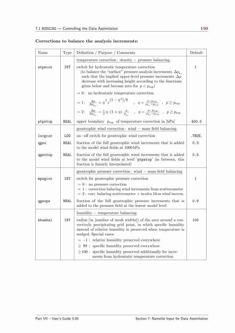
7.1 NUDGING — Controlling the Data Assimilation 150
Corrections to balance the analysis increments:
Name Type Definition / Purpose / Comments Default
temperature correction : density − pressure balancing
ntpscor INT switch for hydrostatic temperature correction(to balance the “surface” pressure analysis increments ∆p
ks
such that the implied upper-level pressure increments ∆pdecrease with increasing height according to the functionsgiven below and become zero for p < ptop)
= 0 : no hydrostatic temperature correction
= 1 : ∆p∆p
ks
= η2e(1− η 3)/8
, η =p−ptop
pks−ptop, p ≥ ptop
= 2 : ∆p∆p
ks
= 12 η ·(1 + η)· p
pks
, η =p−ptop
pks−ptop, p ≥ ptop
1
ptpstop REAL upper boundary ptop of temperature correction in [hPa] 400.0
geostrophic wind correction : wind − mass field balancing
luvgcor LOG on−off switch for geostrophic wind correction .TRUE.
qgeo REAL fraction of the full geostrophic wind increments that is addedto the model wind fields at 1000 hPa
0.3
qgeotop REAL fraction of the full geostrophic wind increments that is addedto the model wind fields at level ’ptpstop’ (in between, thisfraction is linearly interpolated)
0.5
geostrophic pressure correction : wind − mass field balancing
mpsgcor INT switch for geostrophic pressure correction
= 0 : no pressure correction= 1 : correction balacing wind increments from scatterometer= 2 : corr. balacing scatterometer + in-situ 10-m wind increm.
1
qgeops REAL fraction of the full geostrophic pressure increments that isadded to the pressure field at the lowest model level
0.9
humidity − temperature balancing
khumbal INT radius (in [number of mesh widths]) of the area around a con-vectively precipitating grid point, in which specific humidityinstead of relative humidity is preserved when temperature isnudged. Special cases:
= - 1 : relative humidity preserved everywhere
≥ 99 : specific humidity preserved everywhere
≥ 100 : specific humidity preserved additionally for incre-ments from hydrostatic temperature correction
100
Part VII – User’s Guide 5.05 Section 7: Namelist Input for Data Assimilation

7.1 NUDGING — Controlling the Data Assimilation 151
Several of the subsequent blocks of descriptions of NAMELIST parameters contain variableswhich are arrays of 4 elements. These always relate to the following physical quantities:
1: horizontal wind (u , v)
2: ’surface’ pressure ps ; this relates to station pressure observations and to pressure(observation and analysis) increments at the lowest model level
3: temperature T
4: humidity f
Nudging coefficients:
Name Type Definition / Purpose / Comments Default
gnudg(4) REAL nudging coefficients in [1/s]for radiosonde data
6 ·10−4 , 1.2 ·10−3 , 6 ·10−4 , 6 ·10−4
gnudgar(4) REAL nudging coefficients in [1/s]for aircraft data
6 ·10−4 , 0. , 6 ·10−4 , 0.
gnudgar(4) REAL nudging coefficients in [1/s]for MODE-S data
6 ·10−4 , 0. , 6 ·10−4 , 0.
gnudgsu(4) REAL nudging coefficients in [1/s]for surface-level data
6 ·10−4 , 1.2 ·10−3 , 0. , 6 ·10−4
gnudggp REAL nudging coefficient in [1/s]for GPS-derived IWV
0.
Part VII – User’s Guide 5.05 Section 7: Namelist Input for Data Assimilation
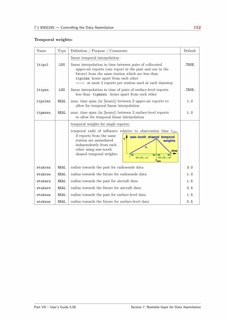
7.1 NUDGING — Controlling the Data Assimilation 152
Temporal weights:
Name Type Definition / Purpose / Comments Default
linear temporal interpolation :
ltipol LOG linear interpolation in time between pairs of collocatedupper-air reports (one report in the past and one in thefuture) from the same station which are less thantipolmx hours apart from each other==> at most 2 reports per station used at each timestep
.TRUE.
ltipsu LOG linear interpolation in time of pairs of surface-level reportsless than tipmxsu hours apart from each other
.TRUE.
tipolmx REAL max. time span (in [hours]) between 2 upper-air reports toallow for temporal linear interpolation
1.0
tipmxsu REAL max. time span (in [hours]) between 2 surface-level reportsto allow for temporal linear interpolation
1.0
temporal weights for single reports:
temporal radii of influence relative to observation time tobs,
wtuk..a wtuk..etobs
time
saw−tooth shaped temporal
weights1
wt
if reports from the samestation are assimilatedindependently from eachother using saw-toothshaped temporal weights:
wtukrsa REAL radius towards the past for radiosonde data 3.0
wtukrse REAL radius towards the future for radiosonde data 1.0
wtukara REAL radius towards the past for aircraft data 1.5
wtukare REAL radius towards the future for aircraft data 0.5
wtuksua REAL radius towards the past for surface-level data 1.5
wtuksue REAL radius towards the future for surface-level data 0.5
Part VII – User’s Guide 5.05 Section 7: Namelist Input for Data Assimilation
7.1 NUDGING — Controlling the Data Assimilation 153
Spatial weights, basic mode of spreading:
Name Type Definition / Purpose / Comments Default
msprpar INT switch specifying the surfaces along which upper-airobservation increments are (primarily) spread
= 0: spreading along model levels==> vertical weights depend approximately on
differences in log-pressure (exactly on differ-ences in scaled height) between the point POI ,for which the observation increment is valid,and the target level at the horizontal locationof the observation
= 1: spreading along horizontal surfaces==> vertical weights depend approximately on
log-pressure differences between point POI
and the target grid point
= 2: spreading along isentropic surfaces==> vertical weights depend on potential tempera-
ture differences between point POI and thetarget grid point
1
msprpsu INT switch specifying the surface along which surface-levelobservation increments are (primarily) spread
= 0: spreading along model levels= 1: spreading along horizontal surfaces= 2: spreading along isentropic surfaces
(for msprpsu , point POI is always a grid pointat the lowest full model level)
0
A “target grid point” is any model grid point for which the analysis increments and hencethe influence (or weight) of any observation is to be computed.
Part VII – User’s Guide 5.05 Section 7: Namelist Input for Data Assimilation
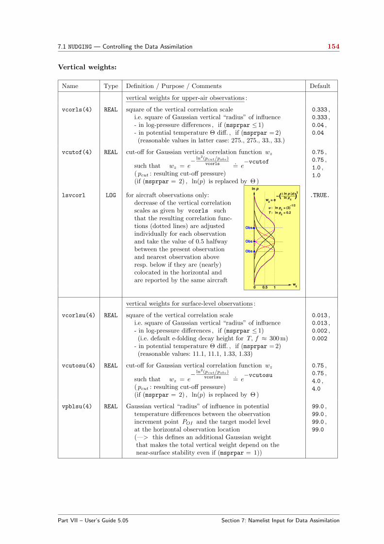
7.1 NUDGING — Controlling the Data Assimilation 154
Vertical weights:
Name Type Definition / Purpose / Comments Default
vertical weights for upper-air observations :
vcorls(4) REAL square of the vertical correlation scalei.e. square of Gaussian vertical “radius” of influence- in log-pressure differences , if (msprpar ≤ 1)- in potential temperature Θ diff. , if (msprpar = 2)(reasonable values in latter case: 275., 275., 33., 33.)
0.333 ,0.333 ,0.04 ,0.04
vcutof(4) REAL cut-off for Gaussian vertical correlation function wz
such that wz = e− ln2(pcut/pobs)
vcorls .= e−vcutof
( pcut : resulting cut-off pressure)(if (msprpar = 2) , ln(p) is replaced by Θ )
wz0.5 10
wz
= e( )−
∆ ln p (z)
ln p
2
c
T : ln p = 0.2c
u : ln p = (3)c
−1/2
ln p
Obs
Obs
Obs
0.75 ,0.75 ,1.0 ,1.0
lsvcorl LOG for aircraft observations only:decrease of the vertical correlationscales as given by vcorls suchthat the resulting correlation func-tions (dotted lines) are adjustedindividually for each observationand take the value of 0.5 halfwaybetween the present observationand nearest observation aboveresp. below if they are (nearly)colocated in the horizontal andare reported by the same aircraft
.TRUE.
vertical weights for surface-level observations :
vcorlsu(4) REAL square of the vertical correlation scalei.e. square of Gaussian vertical “radius” of influence- in log-pressure differences , if (msprpar ≤ 1)(i.e. default e-folding decay height for T, f ≈ 300 m)
- in potential temperature Θ diff. , if (msprpar = 2)(reasonable values: 11.1, 11.1, 1.33, 1.33)
0.013 ,0.013 ,0.002 ,0.002
vcutosu(4) REAL cut-off for Gaussian vertical correlation function wz
such that wz = e− ln2(pcut/pobs)
vcorlsu .= e−vcutosu
( pcut : resulting cut-off pressure)(if (msprpar = 2) , ln(p) is replaced by Θ )
0.75 ,0.75 ,4.0 ,4.0
vpblsu(4) REAL Gaussian vertical “radius” of influence in potentialtemperature differences between the observationincrement point POI and the target model levelat the horizontal observation location(—> this defines an additional Gaussian weightthat makes the total vertical weight depend on thenear-surface stability even if (msprpar = 1))
99.0 ,99.0 ,99.0 ,99.0
Part VII – User’s Guide 5.05 Section 7: Namelist Input for Data Assimilation
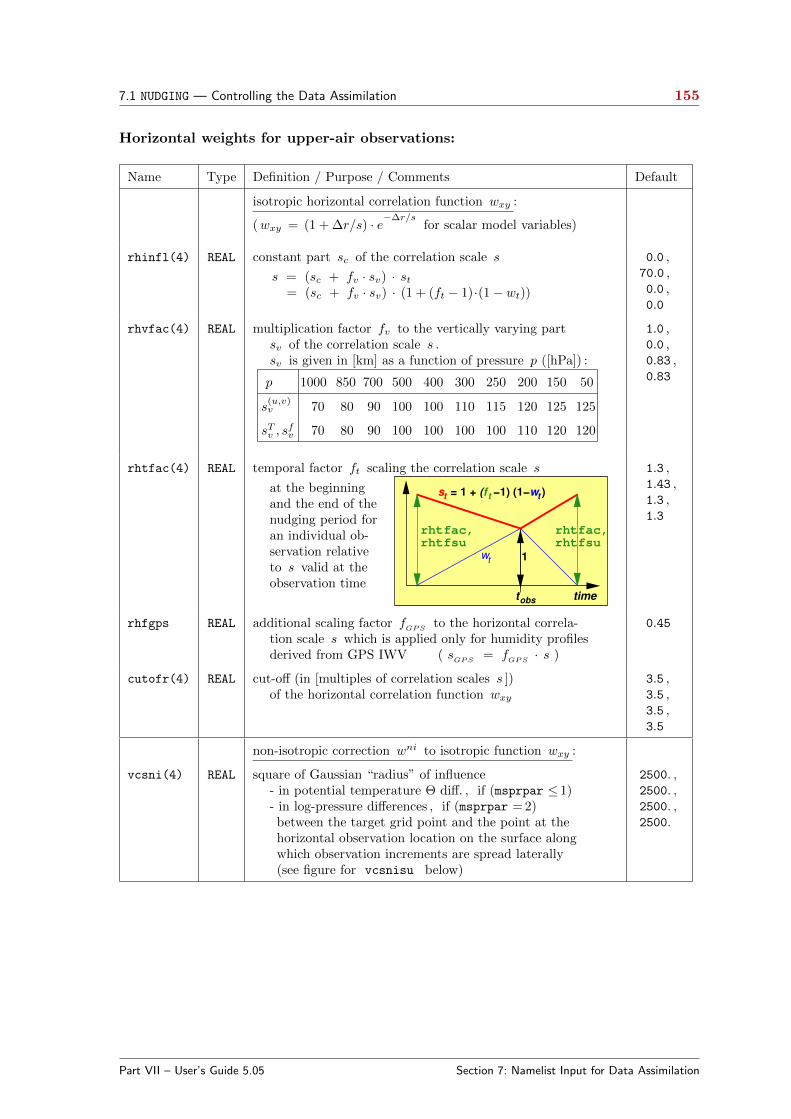
7.1 NUDGING — Controlling the Data Assimilation 155
Horizontal weights for upper-air observations:
Name Type Definition / Purpose / Comments Default
isotropic horizontal correlation function wxy :
(wxy = (1 + ∆r/s) · e−∆r/sfor scalar model variables)
rhinfl(4) REAL constant part sc of the correlation scale s
s = (sc + fv · sv) · st= (sc + fv · sv) · (1 + (ft − 1)·(1− wt))
0.0 ,70.0 ,0.0 ,0.0
rhvfac(4) REAL multiplication factor fv to the vertically varying partsv of the correlation scale s .sv is given in [km] as a function of pressure p ([hPa]) :
p 1000 850 700 500 400 300 250 200 150 50
s(u,v)v 70 80 90 100 100 110 115 120 125 125
sTv , sfv 70 80 90 100 100 100 100 110 120 120
1.0 ,0.0 ,0.83 ,0.83
rhtfac(4) REAL temporal factor ft scaling the correlation scale s
tobs time
1
rhtfac,
rhtfsu
s = 1 + (f −1) (1−w )t t t
wt
rhtfac,
rhtfsu
at the beginningand the end of thenudging period foran individual ob-servation relativeto s valid at theobservation time
1.3 ,1.43 ,1.3 ,1.3
rhfgps REAL additional scaling factor fGPS
to the horizontal correla-tion scale s which is applied only for humidity profilesderived from GPS IWV ( s
GPS= f
GPS· s )
0.45
cutofr(4) REAL cut-off (in [multiples of correlation scales s ])of the horizontal correlation function wxy
3.5 ,3.5 ,3.5 ,3.5
non-isotropic correction wni to isotropic function wxy :
vcsni(4) REAL square of Gaussian “radius” of influence- in potential temperature Θ diff. , if (msprpar ≤ 1)- in log-pressure differences , if (msprpar = 2)between the target grid point and the point at thehorizontal observation location on the surface alongwhich observation increments are spread laterally(see figure for vcsnisu below)
2500. ,2500. ,2500. ,2500.
Part VII – User’s Guide 5.05 Section 7: Namelist Input for Data Assimilation

7.1 NUDGING — Controlling the Data Assimilation 156
Horizontal weights for surface-level observations:
Name Type Definition / Purpose / Comments Default
isotropic horizontal correlation function wxy :
(wxy = (1 + ∆r/s) · e−∆r/sfor scalar model variables)
rhiflsu(4) REAL constant part sc of the correlation scale s (in [km])
s = sc · st = sc · (1 + (ft − 1)·(1− wt))
(wt : temporal weight)
70.0 ,70.0 ,100.0 ,70.0
rhtfsu(4) REAL temporal factor ft scaling the correlation scale sat the beginning and the end of the nudging periodfor an individual observation relative to s valid at theobservation time (see figure for rhtfac above)
1.0 ,1.43 ,1.0 ,1.0
cutofsu(4) REAL cut-off (in [multiples of correlation scales s ])of the horizontal correlation function wxy
2.0 ,3.5 ,2.0 ,2.0
non-isotropic correction wni to isotropic function wxy :
vcsnisu(4) REAL square of Gaussian ’radius’ of influence- in potential temperature differences
i.e. wni = e− (∆Θ)2
vcsnisu if (msprpsu ≤ 1)- in log-pressure differences , if (msprpsu = 2)
between the target grid point and the point at thehorizontal observation location on the surface alongwhich observation increments are spread laterally
888888888888888888888888888888888888888888888888888888888888888888888888888888888888888888888888888888888888888888888888888888888888888888888888888888888888888888888888888888888888888888888
.
mounta
in
vertical spreading −−> wz
observation increment
∆r ∆r
∆Θ
.
.
.non−isotropic correction −−> wni
isentropes
inversion
model levels
target grid point
isotropic lateralspreading−−> wxy
∆Θ
∆z ,∆Θ
spreading of surface-level observation incrementsalong model levels (msprpsu = 0)
2500. ,2500. ,
9. ,9.
rhfpsdd REAL for scaling horizontal correlation scale for surface pressure data 1.0
Part VII – User’s Guide 5.05 Section 7: Namelist Input for Data Assimilation
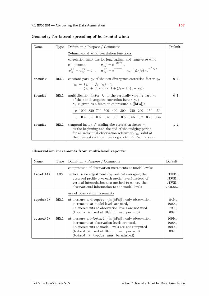
7.1 NUDGING — Controlling the Data Assimilation 157
Geometry for lateral spreading of horizontal wind:
Name Type Definition / Purpose / Comments Default
2-dimensional wind correlation functions :
correlation functions for longitudinal and transverse wind
components wLL
xy = e−∆r/s
,
wLT
xy = wTL
xy = 0 , wTT
xy = e−∆r/s − γn · (∆r/s) · e
−∆r/s
cnondiv REAL constant part γc of the non-divergence correction factor γn
γn = (γc + fv · γv) · γt= (γc + fv · γv) · (1 + (ft − 1)·(1− wt))
0.1
fnondiv REAL multiplication factor fv to the vertically varying part γvof the non-divergence correction factor γn ;γv is given as a function of pressure p ([hPa]) :
p 1000 850 700 500 400 300 250 200 150 50
γv 0.4 0.5 0.5 0.5 0.5 0.6 0.65 0.7 0.75 0.75
0.8
tnondiv REAL temporal factor ft scaling the correction factor γnat the beginning and the end of the nudging periodfor an individual observation relative to γn valid atthe observation time (analogous to rhtfac above)
1.1
Observation increments from multi-level reports:
Name Type Definition / Purpose / Comments Default
computation of observation increments at model levels :
lscadj(4) LOG vertical scale adjustment (by vertical averaging theobserved profile over each model layer) instead ofvertical interpolation as a method to convey theobservational information to the model levels
.TRUE. ,
.TRUE. ,
.TRUE. ,.FALSE.
use of observation increments :
topobs(4) REAL at pressure p < topobs (in [hPa]) , only observationincrements at model levels are used,i.e. increments at observation levels are not used(topobs is fixed at 1099., if msprpar = 0)
849. ,1099. ,799. ,699.
botmod(4) REAL at pressure p > botmod (in [hPa]) , only observationincrements at observation levels are used,i.e. increments at model levels are not computed(botmod is fixed at 1099., if msprpar = 0)(botmod ≥ topobs must be satisfied)
1099. ,1099. ,1099. ,899.
Part VII – User’s Guide 5.05 Section 7: Namelist Input for Data Assimilation
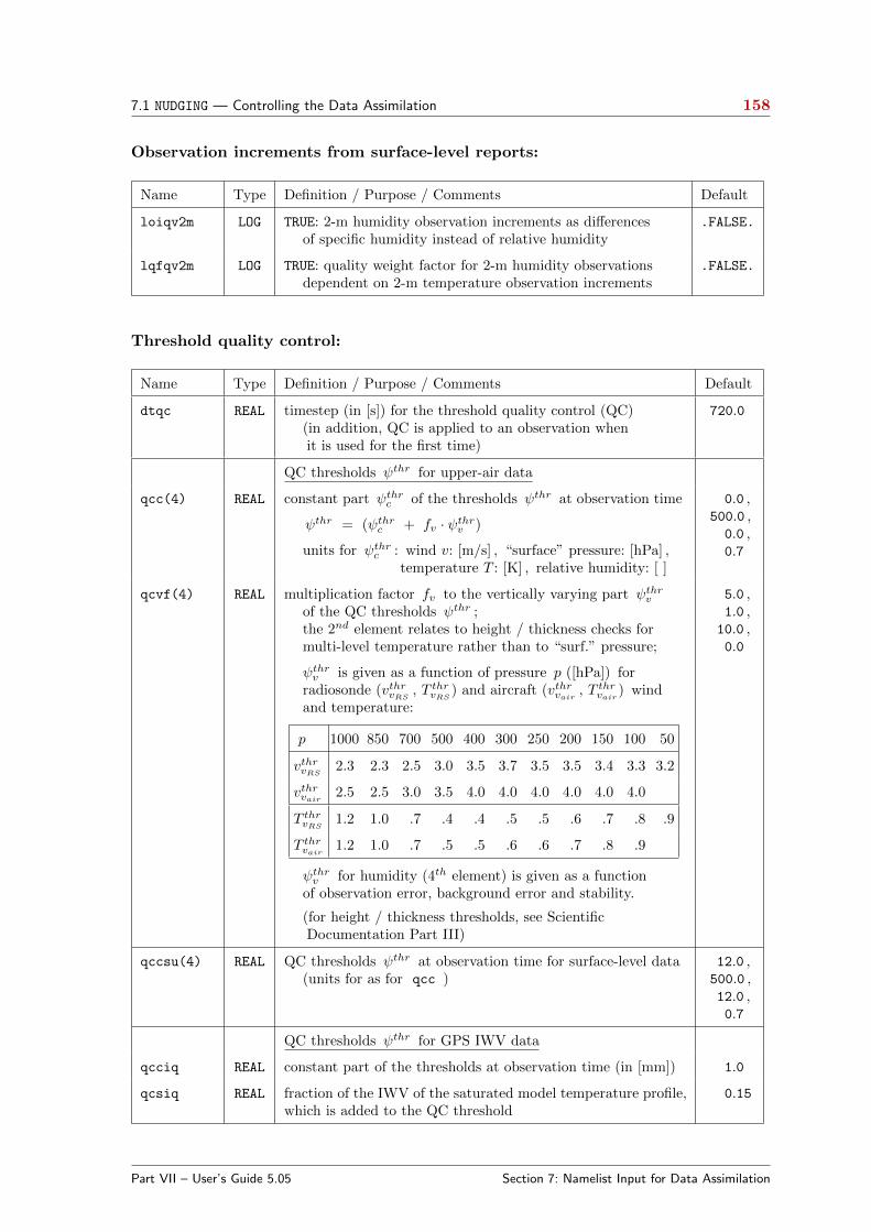
7.1 NUDGING — Controlling the Data Assimilation 158
Observation increments from surface-level reports:
Name Type Definition / Purpose / Comments Default
loiqv2m LOG TRUE: 2-m humidity observation increments as differencesof specific humidity instead of relative humidity
.FALSE.
lqfqv2m LOG TRUE: quality weight factor for 2-m humidity observationsdependent on 2-m temperature observation increments
.FALSE.
Threshold quality control:
Name Type Definition / Purpose / Comments Default
dtqc REAL timestep (in [s]) for the threshold quality control (QC)(in addition, QC is applied to an observation whenit is used for the first time)
720.0
QC thresholds ψthr for upper-air data
qcc(4) REAL constant part ψthrc of the thresholds ψthr at observation time
ψthr = (ψthrc + fv · ψthr
v )
units for ψthrc : wind v: [m/s] , “surface” pressure: [hPa] ,
temperature T : [K] , relative humidity: [ ]
0.0 ,500.0 ,0.0 ,0.7
qcvf(4) REAL multiplication factor fv to the vertically varying part ψthrv
of the QC thresholds ψthr ;the 2nd element relates to height / thickness checks formulti-level temperature rather than to “surf.” pressure;
ψthrv is given as a function of pressure p ([hPa]) for
radiosonde (vthrvRS, T thr
vRS) and aircraft (vthrvair
, T thrvair
) windand temperature:
p 1000 850 700 500 400 300 250 200 150 100 50
vthrvRS2.3 2.3 2.5 3.0 3.5 3.7 3.5 3.5 3.4 3.3 3.2
vthrvair2.5 2.5 3.0 3.5 4.0 4.0 4.0 4.0 4.0 4.0
T thrvRS
1.2 1.0 .7 .4 .4 .5 .5 .6 .7 .8 .9
T thrvair
1.2 1.0 .7 .5 .5 .6 .6 .7 .8 .9
ψthrv for humidity (4th element) is given as a function
of observation error, background error and stability.
(for height / thickness thresholds, see ScientificDocumentation Part III)
5.0 ,1.0 ,
10.0 ,0.0
qccsu(4) REAL QC thresholds ψthr at observation time for surface-level data(units for as for qcc )
12.0 ,500.0 ,12.0 ,0.7
QC thresholds ψthr for GPS IWV data
qcciq REAL constant part of the thresholds at observation time (in [mm]) 1.0
qcsiq REAL fraction of the IWV of the saturated model temperature profile,which is added to the QC threshold
0.15
Part VII – User’s Guide 5.05 Section 7: Namelist Input for Data Assimilation

7.1 NUDGING — Controlling the Data Assimilation 159
Quality weights for observations:
Name Type Definition / Purpose / Comments Default
doromx (4) REAL cut-off and Gaussian “radius” in [m] for reduction factor εzwhich is part of quality weight ε for surface-levelobservations:
|fD
∆z| ≤ doromx : εz = e−(fD·∆z
doromx
)2
(for ps only)
|fD
∆z| ≤ doromx : εz = 1 (for the other variables)
|fD
∆z| > doromx : εz = 0 (applied to all variables)
where ∆z = zobs− zmod : difference (in [m]) between stationheight zobs and model orography zmod
(for ps : zmod = height of lowest model level)
and fD
= 4 for ps if ∆z < 0 (i.e. if extrapolating)fD
= 1 otherwise
—> surface-level data are neglected if |fD
∆z| > doromx !
100.0 ,150.0 ,150.0 ,150.0
qcfpst REAL maximum enhancement factor of the (quality) weight forsurface pressure observations due to observed 3-hourlysurface pressure tendency ∂t ps
(qcfpst is applied if |∂t ps| ≥ 25 hPa ; the enhance-ment decreases linearly with decreasing |∂t ps| to 1 for|∂t ps| ≤ 3 hPa)
1.5
Use of observations and reports:
Name Type Definition / Purpose / Comments Default
altopsu (4) REAL surface-level observations above height altopsu (in [m]) areneglected;if altopsu = 0.0, all surface-level observations assigned to landgrid points are neglected.
100.
5000.
5000.
5000.
zlimv10(3) REAL additional limits for the use of 10-m wind observations:
1,2: positive resp. negative scaled Laplacian of orography[m];
3: surface roughness length [m].
(Introduced in Version 5.04d).
400.0
800.0
5.1
thairh REAL for contructing multi-level reports (’piecewise profiles’) fromsingle-level aircraft reports: maximum horizontal distance in[km] between the resulting multi-level report and the originallocation of any single-level report included in this multi-levelreport
20.
lgpsbias LOG This switch has been eliminated in Version 5.4.seasonal daytime-dependent bias correction applied to GPS-derived IWV (integrated water vapour) data
.FALSE.
Part VII – User’s Guide 5.05 Section 7: Namelist Input for Data Assimilation

7.1 NUDGING — Controlling the Data Assimilation 160
Name Type Definition / Purpose / Comments Default
mqcorr92 INT switch for bias correction for Vaisala RS92 radiosonde humidity
0: no correction for humidity
1: correction of solar radiation bias only
2: correction of total bias (incl. nighttime bias)
0
nolbc INT number of grid rows at the lateral boundaries of the COSMO-Model domain where all reports are neglected
5
observation area : all reports outside of it are neglected
obnlat REAL latitude of northern boundary of observation area ([deg.]) 90.
obslat REAL latitude of southern boundary of observation area ([deg.]) -90.
obwlon REAL longitude of western boundary of observation area ([deg.]) 180.
obelon REAL longitude of eastern boundary of observation area ([deg.]) -180.
Use of observation types and code types:
Name Type Definition / Purpose / Comments Default
exclusion area: reports inside of it are neglected if their obser-vation or code type is set to .FALSE.
exnlat REAL latitude of northern boundary of exclusion area ([deg.]) 90.
exslat REAL latitude of southern boundary of exclusion area ([deg.]) - 90.
exwlon REAL longitude of western boundary of exclusion area ([deg.]) - 180.
exelon REAL longitude of eastern boundary of exclusion area ([deg.]) 180.
observation type: reports inside the exclusion area are set passiveif their type is set to .FALSE.
lsynop LOG observation type SYNOP .TRUE.
laircf LOG observation type AIREP (aircraft) .TRUE.
lsatob LOG observation type SATOB .FALSE.
ldribu LOG observation type DRIBU (drifting buoy) .TRUE.
ltemp LOG observation type TEMP .TRUE.
lpilot LOG observation type PILOT .TRUE.
lsatem LOG observation type SATEM .FALSE.
lgps LOG observation type GPS IWV .FALSE.
lgnssstd LOG observation type GPS STD/ZTD(Introduced in Version 5.04d).
.FALSE.
lscatt LOG observation type SCATT (scatterometer) .TRUE.
Part VII – User’s Guide 5.05 Section 7: Namelist Input for Data Assimilation

7.1 NUDGING — Controlling the Data Assimilation 161
Name Type Definition / Purpose / Comments Default
code type: reports inside the exclusion area are set passiveif their code type is set to .FALSE.
lcd011 LOG SYNOP code 11 (manual land) .TRUE.
lcd014 LOG SYNOP code 14 (autom. land) .TRUE.
lcd021 LOG SYNOP code 21 (manual ship) .TRUE.
lcd022 LOG SYNOP code 22 (abbrev. ship) .TRUE.
lcd023 LOG SYNOP code 23 (reduced ship) .TRUE.
lcd024 LOG SYNOP code 24 (autom. ship) .TRUE.
lcd140 LOG SYNOP code 140 (METAR) .TRUE.
lcd041 LOG AIREP code 41 (CODAR) .TRUE.
lcd141 LOG AIREP code 141 (AIREP) .TRUE.
lcd241 LOG AIREP code 241 (constant level balloon) .TRUE.
lcd144 LOG AIREP code 144 (AMDAR) .TRUE.
lcd146 LOG AIREP code 146 (MODE-S) .TRUE.
lcd244 LOG AIREP code 244 (ACAR) .TRUE.
lcd088 LOG SATOB code 88 (SATOB) .TRUE.
lcd188 LOG SATOB code 188 (SST) .TRUE.
lcd063 LOG DRIBU code 63 (bathy sphere) .TRUE.
lcd064 LOG DRIBU code 64 (TESAC) .TRUE.
lcd165 LOG DRIBU code 165 (drifting buoy) .TRUE.
lcd035 LOG TEMP code 35 (land radiosonde) .TRUE.
lcd036 LOG TEMP code 36 (ship radiosonde) .TRUE.
lcd037 LOG TEMP code 37 (mobile radiosonde) .TRUE.
lcd135 LOG TEMP code 135 (drop sonde) .TRUE.
lcd039 LOG TEMP code 39 (land rocket) .TRUE.
lcd040 LOG TEMP code 40 (ship rocket) .TRUE.
lcd032 LOG PILOT code 32 (land PILOT) .TRUE.
lcd033 LOG PILOT code 33 (ship PILOT) .TRUE.
lcd038 LOG PILOT code 38 (mobile PILOT) .TRUE.
lcd132 LOG PILOT code 132 (European wind profiler) .TRUE.
lcd133 LOG PILOT code 133 (European SODAR / RASS) .TRUE.
lcd136 LOG PILOT code 136 (US wind profiler / RASS) .FALSE.
lcd137 LOG PILOT code 137 (radar VAD) .FALSE.
lcd122 LOG SCATT code 122 (OSCAT) .TRUE.
lcd123 LOG SCATT code 123 (ASCAT) .TRUE.
lcd090 LOG AMV 90 (AMV) .TRUE.
Part VII – User’s Guide 5.05 Section 7: Namelist Input for Data Assimilation

7.1 NUDGING — Controlling the Data Assimilation 162
Name Type Definition / Purpose / Comments Default
lcd096 LOG GPS code 96 (ground-based GPS) ; this code type is usedonly for GPS data read from a specialASCII file in COST-716 format
.TRUE.
igpscen
(20)
INT array of processing centres of GPS reports used actively:
- the order of centres determines the preference in the re-dundancy check; ’-1’ means no active centre
- the numbers Np indicating the processing centres are givenin the WMO Common Code Table C-12 for BUFR/CREXdata (WMO descriptor ’0 01 034’)
- the code types for GPS data (if read from NetCDF files)are set to ’X +Np’ where X=800 or X=900 ; these codetype have to be used e.g. for setting ’iwtyp’
-1,
-1,
. . .
Part VII – User’s Guide 5.05 Section 7: Namelist Input for Data Assimilation
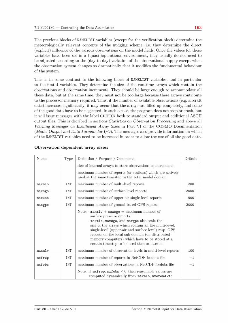
7.1 NUDGING — Controlling the Data Assimilation 163
The previous blocks of NAMELIST variables (except for the verification block) determine themeteorologically relevant contents of the nudging scheme, i.e. they determine the direct(explicit) influence of the various observations on the model fields. Once the values for thesevariables have been set in a (quasi-)operational environment, they usually do not need tobe adjusted according to the (day-to-day) variation of the observational supply except whenthe observation system changes so dramatically that it modifies the fundamental behaviourof the system.
This is in some contrast to the following block of NAMELIST variables, and in particularto the first 4 variables. They determine the size of the run-time arrays which contain theobservations and observation increments. They should be large enough to accommodate allthese data, but at the same time, they must not be too large because these arrays contributeto the processor memory required. Thus, if the number of available observations (e.g. aircraftdata) increases significantly, it may occur that the arrays are filled up completely, and someof the good data have to be neglected. In such a case, the program does not stop or crash, butit will issue messages with the label CAUTION both to standard output and additional ASCIIoutput files. This is decribed in sections Statistics on Observation Processing and above allWarning Messages on Insufficient Array Sizes in Part VI of the COSMO Documentation(Model Output and Data Formats for I/O). The messages also provide information on whichof the NAMELIST variables need to be increased in order to allow the use of all the good data.
Observation dependent array sizes:
Name Type Definition / Purpose / Comments Default
size of internal arrays to store observations or increments
maximum number of reports (or stations) which are activelyused at the same timestep in the total model domain
maxmlo INT maximum number of multi-level reports 300
maxsgo INT maximum number of surface-level reports 3000
maxuso INT maximum number of upper-air single-level reports 900
maxgpo INT maximum number of ground-based GPS reports 3000
Note: - maxmlo + maxsgo = maximum number ofsurface pressure reports
- maxmlo, maxsgo, and maxgpo also scale thesize of the arrays which contain all the multi-level,single-level (upper-air and surface level) resp. GPSreports on the local sub-domain (on distributed-memory computers) which have to be stored at acertain timestep to be used then or later on
maxmlv INT maximum number of observation levels in multi-level reports 100
mxfrep INT maximum number of reports in NetCDF feedobs file −1
mxfobs INT maximum number of observations in NetCDF feedobs file −1
Note: if mxfrep, mxfobs ≤ 0 then reasonable values arecomputed dynamically from maxmlo, hverend etc.
Part VII – User’s Guide 5.05 Section 7: Namelist Input for Data Assimilation

7.1 NUDGING — Controlling the Data Assimilation 164
Directory and file names related to nudging:
Name Type Definition / Purpose / Comments Default
itype obfile INT This switch has been eliminated in Version 5.4.Only NetCDF files are possible now, AOF files are no moresupported.
—
yaofpath CHAR This switch has been eliminated in Version 5.4. —
ycdfdir CHAR directory, where NetCDF observation input files and theblacklist file reside
’./’
yfofdir CHAR directory for output of NetCDF fof file ’./’
Diagnostic output:
The ASCII files that are produced by the diagnostic output are explained in detail in PartVI of the COSMO Documentation: Model Output and Data Formats for I/O.
Name Type Definition / Purpose / Comments Default
lprodr LOG diagnostic print about observation data record ODRon file YUOBSDR
.TRUE.
ionl INT grid point coordinates for control output on file YUPRINT 167
jonl INT 103
ionl2 INT grid point coordinates for further control output 167
jonl2 INT 103
All these switches have been eliminated in Version 5.4.
lpraof LOG diagnostic print of analysis observation file AOF on file YUAOFEX .FALSE.
dinlat REAL latitude of northern boundary of diagnostic print area ([deg.]) 0.
dislat REAL latitude of southern boundary of diagnostic print area ([deg.]) 0.
diwlon REAL longitude of western boundary of diagnostic print area ([deg.]) 0.
dielon REAL longitude of eastern boundary of diagnostic print area ([deg.]) 0.
noctrq INT observation or code type of reports to be printed;if (noctrq = 9) then print all report (types)
9
Part VII – User’s Guide 5.05 Section 7: Namelist Input for Data Assimilation

7.1 NUDGING — Controlling the Data Assimilation 165
The following variables and are relevant only if ’lsurfa = .TRUE.’ .
2-dimensional analyses derived from observations:
Name Type Definition / Purpose / Comments Default
2-m temperature analyses
lt2m LOG 2-m temperature field is analysed (if true) .FALSE.
ht2a REAL time (in [hours]) of first 2-m temperature analysisrelative to initial time of model run
999.
ht2i REAL time increment (in [hours]) between successive2-m temperature analyses
999.
2-m relative humidity analyses
lrh2m LOG 2-m relative humidity field is analysed .FALSE.
hh2a REAL time (in [hours]) of first 2-m relative humidity analysisrelative to initial time of model run
999.
hh2i REAL time increment (in [hours]) between successive2-m relative humidity analyses
999.
10-m wind analyses
lff10m LOG 10-m wind speed is analysed .FALSE.
hffa REAL time (in [hours]) of first 10-m wind analysisrelative to initial time of model run
999.
hffi REAL time increment (in [hours]) between successive10-m wind analyses
999.
precipitation analyses
lprecp LOG precipitation is analysed .FALSE.
hprc REAL time (in [hours]) of analysis of precipitation sumrelative to initial time of model run
999.
raintp REAL time period (in [hours]) over which precipitation is summed up 12.
ldiasa LOG diagnostics on 2-dimensional surface analyses on file YUSURF .FALSE.
Part VII – User’s Guide 5.05 Section 7: Namelist Input for Data Assimilation
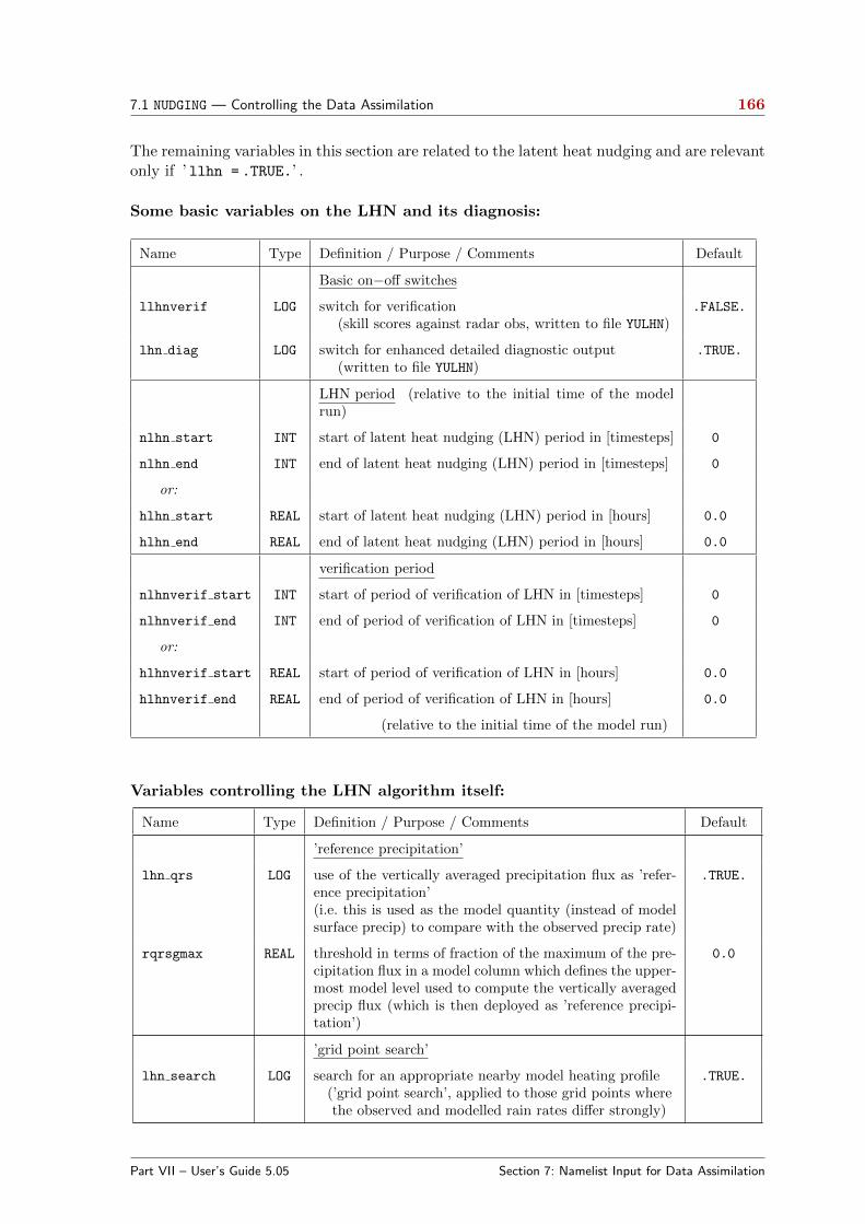
7.1 NUDGING — Controlling the Data Assimilation 166
The remaining variables in this section are related to the latent heat nudging and are relevantonly if ’ llhn = .TRUE.’ .
Some basic variables on the LHN and its diagnosis:
Name Type Definition / Purpose / Comments Default
Basic on−off switches
llhnverif LOG switch for verification(skill scores against radar obs, written to file YULHN)
.FALSE.
lhn diag LOG switch for enhanced detailed diagnostic output(written to file YULHN)
.TRUE.
LHN period (relative to the initial time of the modelrun)
nlhn start INT start of latent heat nudging (LHN) period in [timesteps] 0
nlhn end INT end of latent heat nudging (LHN) period in [timesteps] 0
or:
hlhn start REAL start of latent heat nudging (LHN) period in [hours] 0.0
hlhn end REAL end of latent heat nudging (LHN) period in [hours] 0.0
verification period
nlhnverif start INT start of period of verification of LHN in [timesteps] 0
nlhnverif end INT end of period of verification of LHN in [timesteps] 0
or:
hlhnverif start REAL start of period of verification of LHN in [hours] 0.0
hlhnverif end REAL end of period of verification of LHN in [hours] 0.0
(relative to the initial time of the model run)
Variables controlling the LHN algorithm itself:
Name Type Definition / Purpose / Comments Default
’reference precipitation’
lhn qrs LOG use of the vertically averaged precipitation flux as ’refer-ence precipitation’(i.e. this is used as the model quantity (instead of modelsurface precip) to compare with the observed precip rate)
.TRUE.
rqrsgmax REAL threshold in terms of fraction of the maximum of the pre-cipitation flux in a model column which defines the upper-most model level used to compute the vertically averagedprecip flux (which is then deployed as ’reference precipi-tation’)
0.0
’grid point search’
lhn search LOG search for an appropriate nearby model heating profile(’grid point search’, applied to those grid points wherethe observed and modelled rain rates differ strongly)
.TRUE.
Part VII – User’s Guide 5.05 Section 7: Namelist Input for Data Assimilation
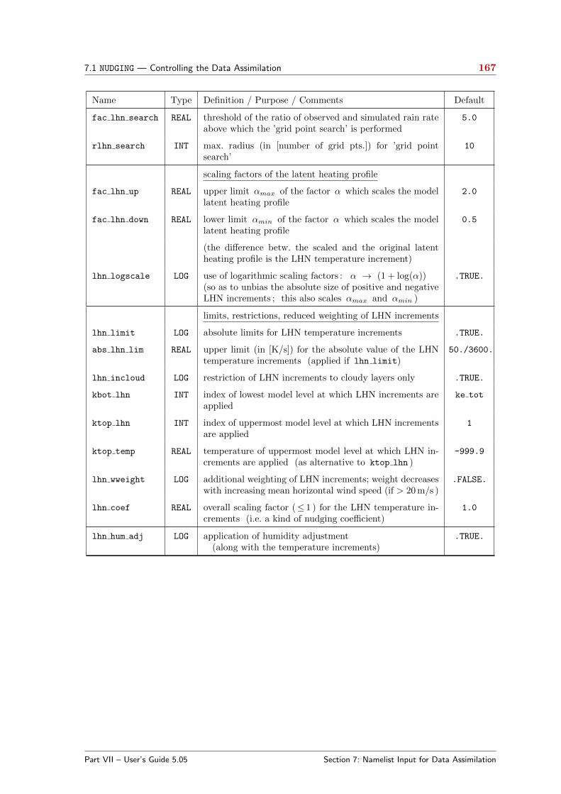
7.1 NUDGING — Controlling the Data Assimilation 167
Name Type Definition / Purpose / Comments Default
fac lhn search REAL threshold of the ratio of observed and simulated rain rateabove which the ’grid point search’ is performed
5.0
rlhn search INT max. radius (in [number of grid pts.]) for ’grid pointsearch’
10
scaling factors of the latent heating profile
fac lhn up REAL upper limit αmax of the factor α which scales the modellatent heating profile
2.0
fac lhn down REAL lower limit αmin of the factor α which scales the modellatent heating profile
0.5
(the difference betw. the scaled and the original latentheating profile is the LHN temperature increment)
lhn logscale LOG use of logarithmic scaling factors : α → (1 + log(α))(so as to unbias the absolute size of positive and negativeLHN increments ; this also scales αmax and αmin )
.TRUE.
limits, restrictions, reduced weighting of LHN increments
lhn limit LOG absolute limits for LHN temperature increments .TRUE.
abs lhn lim REAL upper limit (in [K/s]) for the absolute value of the LHNtemperature increments (applied if lhn limit)
50./3600.
lhn incloud LOG restriction of LHN increments to cloudy layers only .TRUE.
kbot lhn INT index of lowest model level at which LHN increments areapplied
ke tot
ktop lhn INT index of uppermost model level at which LHN incrementsare applied
1
ktop temp REAL temperature of uppermost model level at which LHN in-crements are applied (as alternative to ktop lhn )
-999.9
lhn wweight LOG additional weighting of LHN increments; weight decreaseswith increasing mean horizontal wind speed (if > 20 m/s )
.FALSE.
lhn coef REAL overall scaling factor (≤ 1 ) for the LHN temperature in-crements (i.e. a kind of nudging coefficient)
1.0
lhn hum adj LOG application of humidity adjustment(along with the temperature increments)
.TRUE.
Part VII – User’s Guide 5.05 Section 7: Namelist Input for Data Assimilation

7.1 NUDGING — Controlling the Data Assimilation 168
Observation and file input for LHN:
Name Type Definition / Purpose / Comments Default
spatial filtering
lhn filt LOG vertical filtering of LHN temperature increments .TRUE.
lhn relax LOG horizontal filtering, both of the− (observed and simulated) precipitation fields (input)− LHN temperature increments (output)
.TRUE.
nlhn relax INT number of iterations of (2-grid-point scale) horiz. filtering 2
thresholds and weighting of observation input
thres lhn REAL threshold (in [mm/s]) below which the rain rate is consid-ered to be zero in many aspects within the LHN scheme
0.1/3600.
rad wobs lhn REAL maximum range from radar site with full observationweight (in [km])
100.
lhn spqual LOG use of a spatial quality function of the input rain rates .FALSE.
observation and auxilliary file input
nradar INT maximum number of radar stations in obs input data 33
lhn dt obs REAL time step of the observation input data (in [minutes]) 5.0
noobs date (36) CHAR dates without radar data(as [YYYYMMDDHHTT], where YYYY = year, MM =month, DD = day, HH = hour, TT = minute)
’ ’
lhn black LOG use of a blacklist for radar data(this requires an additional Grib file, see blacklist)
.TRUE.
lhn bright LOG bright band detection (and rejection of flagged data)(this requires radar beam height maps)
.TRUE.
lhn height LOG use of radar beam height maps(this requires an additional Grib file, see height file)
.TRUE.
Name Type Definition / Purpose / Comments Default
directory and file names
radar in CHAR directory in which the radar data files reside ’.’
(incl. blacklist & beam height map files)
blacklist file CHAR file name of blacklist for radar data ’blacklist dx.grib1’
height file CHAR file name of radar beam height maps ’height dx.grib1’
Part VII – User’s Guide 5.05 Section 7: Namelist Input for Data Assimilation
169
Section 8
Special Operators for the DataAssimilation
8.1 The GNSS STD Operator
8.1.1 Input for the GNSS STD Operator
Geoid Undulation
COSMO provides the surface height (field HSURF) and the heights of half levels (field HHL)as heights above mean sea level which are equivalent to heights above geoid. The geoid isrelated to the local gravity field of the Earth and only empirical estimates of the Earth’sgeoid are available. Consequently, there is no general transformation from the geographicalcoordinates provided by COSMO and other reference systems, e. g. used to define satellitedata. It is necessary to translate the heights above geoid to heights above a reference ellipsoid.Such ellipsoidal coordinates can easily be transformed to global Cartesian coordinates andto any other reference system.
The geoid undulation describes the difference between the height above geoid and the heightabove ellipsoid. Several empirical data sets are available and are updated in regular intervals,either because of new gravity data or because the Earth’s gravity field changed. One of themost recent and best resolved data sets is the eigen-6c3stat geoid which is used in COSMO.
The global eigen-6c3stat geoid with a resolution of 0.1◦ can be obtained from the web sitehttp://icgem.gfz-potsdam.de/ICGEM/ICGEM.html. The web server provides the 350 MBASCII file eigen-6c3stat-450553.gdf. The format of the geoid data is described on theweb site and in Forste et al. (2013). It is rather time consuming to read such a large ASCIIfile therefore a netCDF converter was written. The size of the netCDF file is 50 MB and it ispossible to read only the geoid subarray required for the given model domain. The contentsof the netCDF file is described below.
The geoid file is required only if the GNSS STD operator is running.
Part VII – User’s Guide 5.05 Section 8: Special Operators for the Data Assimilation
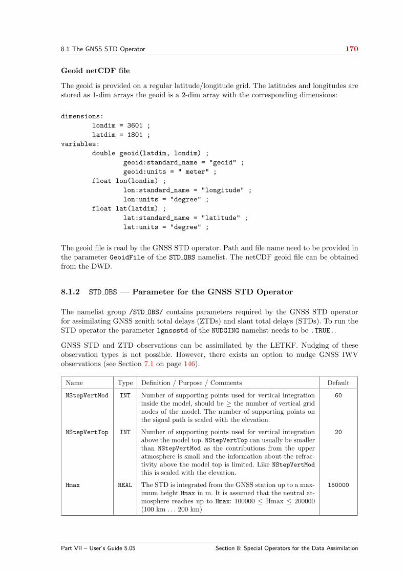
8.1 The GNSS STD Operator 170
Geoid netCDF file
The geoid is provided on a regular latitude/longitude grid. The latitudes and longitudes arestored as 1-dim arrays the geoid is a 2-dim array with the corresponding dimensions:
dimensions:
londim = 3601 ;
latdim = 1801 ;
variables:
double geoid(latdim, londim) ;
geoid:standard_name = "geoid" ;
geoid:units = " meter" ;
float lon(londim) ;
lon:standard_name = "longitude" ;
lon:units = "degree" ;
float lat(latdim) ;
lat:standard_name = "latitude" ;
lat:units = "degree" ;
The geoid file is read by the GNSS STD operator. Path and file name need to be provided inthe parameter GeoidFile of the STD OBS namelist. The netCDF geoid file can be obtainedfrom the DWD.
8.1.2 STD OBS — Parameter for the GNSS STD Operator
The namelist group /STD OBS/ contains parameters required by the GNSS STD operatorfor assimilating GNSS zenith total delays (ZTDs) and slant total delays (STDs). To run theSTD operator the parameter lgnssstd of the NUDGING namelist needs to be .TRUE..
GNSS STD and ZTD observations can be assimilated by the LETKF. Nudging of theseobservation types is not possible. However, there exists an option to nudge GNSS IWVobservations (see Section 7.1 on page 146).
Name Type Definition / Purpose / Comments Default
NStepVertMod INT Number of supporting points used for vertical integrationinside the model, should be ≥ the number of vertical gridnodes of the model. The number of supporting points onthe signal path is scaled with the elevation.
60
NStepVertTop INT Number of supporting points used for vertical integrationabove the model top. NStepVertTop can usually be smallerthan NStepVertMod as the contributions from the upperatmosphere is small and the information about the refrac-tivity above the model top is limited. Like NStepVertMod
this is scaled with the elevation.
20
Hmax REAL The STD is integrated from the GNSS station up to a max-imum height Hmax in m. It is assumed that the neutral at-mosphere reaches up to Hmax: 100000 ≤ Hmax ≤ 200000(100 km . . . 200 km)
150000
Part VII – User’s Guide 5.05 Section 8: Special Operators for the Data Assimilation
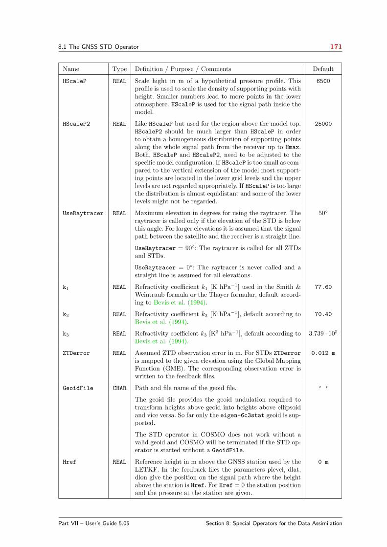
8.1 The GNSS STD Operator 171
Name Type Definition / Purpose / Comments Default
HScaleP REAL Scale hight in m of a hypothetical pressure profile. Thisprofile is used to scale the density of supporting points withheight. Smaller numbers lead to more points in the loweratmosphere. HScaleP is used for the signal path inside themodel.
6500
HScaleP2 REAL Like HScaleP but used for the region above the model top.HScaleP2 should be much larger than HScaleP in orderto obtain a homogeneous distribution of supporting pointsalong the whole signal path from the receiver up to Hmax.Both, HScaleP and HScaleP2, need to be adjusted to thespecific model configuration. If HScaleP is too small as com-pared to the vertical extension of the model most support-ing points are located in the lower grid levels and the upperlevels are not regarded appropriately. If HScaleP is too largethe distribution is almost equidistant and some of the lowerlevels might not be regarded.
25000
UseRaytracer REAL Maximum elevation in degrees for using the raytracer. Theraytracer is called only if the elevation of the STD is belowthis angle. For larger elevations it is assumed that the signalpath between the satellite and the receiver is a straight line.
50◦
UseRaytracer = 90◦: The raytracer is called for all ZTDsand STDs.
UseRaytracer = 0◦: The raytracer is never called and astraight line is assumed for all elevations.
k1 REAL Refractivity coefficient k1 [K hPa−1] used in the Smith &Weintraub formula or the Thayer formular, default accord-ing to Bevis et al. (1994).
77.60
k2 REAL Refractivity coefficient k2 [K hPa−1], default according toBevis et al. (1994).
70.40
k3 REAL Refractivity coefficient k3 [K2 hPa−1], default according toBevis et al. (1994).
3.739 · 105
ZTDerror REAL Assumed ZTD observation error in m. For STDs ZTDerroris mapped to the given elevation using the Global MappingFunction (GME). The corresponding observation error iswritten to the feedback files.
0.012 m
GeoidFile CHAR Path and file name of the geoid file. ’ ’
The geoid file provides the geoid undulation required totransform heights above geoid into heights above ellipsoidand vice versa. So far only the eigen-6c3stat geoid is sup-ported.
The STD operator in COSMO does not work without avalid geoid and COSMO will be terminated if the STD op-erator is started without a GeoidFile.
Href REAL Reference height in m above the GNSS station used by theLETKF. In the feedback files the parameters plevel, dlat,dlon give the position on the signal path where the heightabove the station is Href. For Href = 0 the station positionand the pressure at the station are given.
0 m
Part VII – User’s Guide 5.05 Section 8: Special Operators for the Data Assimilation

8.1 The GNSS STD Operator 172
Name Type Definition / Purpose / Comments Default
MaxSTDobs INT Maximum number of STDs to read/process 100000
MaxZTDobs INT Maximum number of ZTDs to read/process The memoryrequired to read and process the GNSS observations growswith the number of observations and may exceed the avail-able memory. As the number of future observations is un-predictable an upper limit is set in order to guarantee stableoperation.
50000
verbose REAL Verbosity level of program messages. At higher verbositylevels the output of all lower levels will also be provided.This parameter is used by the STD operator only.
0
verbose = 0 (default)
Output limited to some status messages.
verbose = 1
Messages necessary to follow the program flow.
verbose = 2
More messages and output of some important variables.
verbose = 3
Debug mode, huge amount of output.
HORIFile CHAR Path and file name of the GNSS station list. ’ ’
The GNSS station list is required to process STD obser-vations which are provided in a preliminary data format.As STD and ZTD data are processed in the same way theGNSS station list needs to be available even if only ZTDsare used. This parameter will become obsolete as soon asSTD BUFR data are available.
Part VII – User’s Guide 5.05 Section 8: Special Operators for the Data Assimilation
REFERENCES 173
References
Baldauf, M., 2013. A new fast-waves solver for the Runge-Kutta dynamical core. COSMO Technical Report No. 21,Consortium for Small-Scale Modelling, http://www.cosmo-model.org/content/model/documentation/techReports/default.htm.
Baldauf, M., 2014. The COSMO model: towards cloud-resolving NWP. In RecentDevelopments in Numerical Methods for Atmosphere and Ocean Modelling -Proceedings of a Seminar, pp. 107–122. ECMWF, Reading, UK.
Bechtold, P., E. Bazile, F. Guichard, P. Mascart, and E. Richard, 2001. A mass-flux convection scheme for regional and global models. Quart. J. Roy. Meteor. Soc.,127, 869–886.
Bechtold, P., M. Kohler, T. Jung, F. Doblas-Reyes, M. Leutbecher, M. Rod-well, F. Vitart, and G. Balsa, 2008. Advances in simulating atmospheric variabilitywith the ECMWF model: From synoptic to decadal time-scales. Quart. J. Roy. Meteor.Soc., 134, 1337–1351.
Bechtold, P., N. Semane, P. Lopez, J.-P. Chaboureau, A. Beljaars, and N. Bor-mann, 2008. Representing equilibrium and non-equilibrium convection in large-scalemodels. J. Atmos. Sci., 71, 734–753.
Bevis, M., S. Businger, S. Chiswell, T. A. Herring, R. A. Anthes, C. Rocken,and R. H. Ware, 1994. GPS Meteorology: Mapping Zenith Wet Delays onto Pre-cipitable Water. J. Appl. Meteor. 33(3), 379–386.
Davies, H. and R. Turner, 1977. Updating prediction models by dynamical relaxation:An examination of the technique. Quart. J. R. Met. Soc., 103, 225–245.
Dudhia, J., 1993. A nonhydrostatic version of the Penn State / NCAR mesoscale model:Validation tests and simulation of an Atlantic cyclone and cold front. Mon. Wea. Rev.,121, 1493–1513.
Forste, C., S. Bruinsma, J.-C. Marty, F. Flechtner, O. Abrikosov, C. Dahle,J.-M. Lemoine, K. H. Neumayer, R. Biancale, F. Barthelmes, and R. Konig,2013. EIGEN-6C3stat - the newest High Resolution Global Combined GravityField Model based on the 4th Release of the GOCE Direct Approach. Talk, Pots-dam/Toulouse.
Hess, R., 2001. Assimilation of screen-level observations by variational soil moistureanalysis. Meteorol. Atmos. Phys., 77, 155–166.
Jacobsen, I. and E. Heise, 1982. A new economic method for the computation of thesurface temperature in numerical models. Contr. Atmos. Phys., 55, 128–141.
Kessler, E., 1969. On the Distribution and Continuity of water substance in the
Part VII – User’s Guide 5.05 REFERENCES
REFERENCES 174
atmospheric circulations, Volume 32 of Meteorological Monographs Vol. 10. Ameri-can Meteorological Society, Boston.
Klemp, J. and R. Wilhelmson, 1978. The Simulation of Three-dimensional ConvectiveStorm Dynamics. J. Atmos. Sci., 35, 1070–1096.
Liu, X.-D., S. Osher, and T. Chan, 1994. Weighted essentially non-oscillatoryschemes. J. Comput. Phys., 115, 200–212.
Louis, J.-F., 1979. A parametric model of vertical eddy fluxes in the atmosphere. Bound.Layer Meteor., 17, 187–202.
Lynch, P., D. Girard, and V. Ivanovici, 1997. mproving the efficiency of a digitalfiltering scheme. Mon. Wea. Rev., 125, 1976–1982.
Mellor, G. and T. Yamada, 1974. A hierarchy of turbulence closure models for plan-etary boundary layers. J. Atm. Sc., 31, 1791–1806.
Mironov, D., 2008. Parameterization of lakes in numerical weather prediction. De-scription of a lake model. COSMO Technical Report No. 11, Deutscher Wetterdienst,Deutscher Wetterdienst, D-63004 Offenbach, Germany.
Mironov, D. and R. B., 2004. Testing the new ice model for the global NWP systemGME of the German Weather Service. Technical documentation, 1220, WMO, WMO,Geneve, Switzerland.
Muller, E., 1981. Turbulent flux parameterization in a regional-scale model. In ECMWFWorkshop on planetary boundary layer parameterization, pp. 193–220. 25-27 Novem-ber, 1981.
Ritter, B. and J.-F. Geleyn, 1992. A comprehensive radiation scheme for numericalweather prediction models with potential applications in climate simulations. Mon.Wea. Rev., 120, 303–325.
Schaer, C., D. Leuenberger, O. Fuhrer, D. Luthi, and C. Girard, 2002. A newterrain-following vertical coordinate formulation for atmospheric prediction models.Mon. Wea. Rev., 130, 2459–2480.
Schraff, C., 1996. Data assimilation and mesoscale weather prediction: A study with aforecast model for the Alpine region. Publication 56, Swiss Meteorological Institute,Zurich.
Schraff, C., 1997. Mesoscale data assimilation and prediction of low stratus in the Alpineregion. Meteorol. Atmos. Phys., 64, 21–50.
Skamarock, W. and J. Klemp, 1992. The stability of time-split numerical methods forthe hydrostatic and nonhydrostatic elasic equations. Mon. Wea. Rev., 120, 2109–2127.
Skamarock, W., P. Smolarkiewicz, and J. Klemp, 1997. Preconditioned ConjugateGradient Solvers for Helmholtz Equations in Nonhydrostatic Models. Mon. Wea. Rev.,125, 587–599.
Sommeria, G. and J. W. Deardorff, 1977. Subgrid-scale condensation in models ofnon-precipitating clouds. J. Atmos. Sci., 34, 344–355.
Stauffer, D. and N. Seaman, 1990. Use of four-dimensional data assimilation in alimited-area mesoscale model. Part I: Experiments with synoptic-scale data. Mon. Wea.Rev., 118, 1250–1277.
Stauffer, D. and N. Seaman, 1994. Multiscale four-dimensional data assimilation. J.Appl. Meteor., 33, 416–434.
Part VII – User’s Guide 5.05 REFERENCES
REFERENCES 175
Stephan, K., S. Klink, and C. Schraff, 2008. Assimilation of radar-derived rain ratesinto the convective-scale model COSMO-DE at DWD. Quart. J. R. Meteor. Soc., 134,1315–1326.
Thomas, S., C. Girard, G. Doms, and U. Schattler, 2000. Semi-Implicit Schemefor the DWD Lokal-Modell. Meteorol. Atmos. Phys., 73, 105–125.
Tiedtke, M., 1989. A comprehensive mass flux scheme for cumulus parameterization inlarge-scale models. Mon. Wea. Rev., 117, 1779–1799.
Wicker, L. and W. Skamarock, 2002. Time-splitting methods for elastic models usingforward time schemes. Mon. Wea. Rev., 130, 2088–2097.
Part VII – User’s Guide 5.05 REFERENCES