A Demonstration of Data Mining - Win-Vector LLC Demonstration of Data Mining John Mount August 19,...
16
A Demonstration of Data Mining John Mount * August 19, 2009 Abstract We demonstrate the spirit of data mining techniques by working through a simple idealized example. We then use the experience from the example to support a survey of important data mining considerations. 1 Introduction A major industry in our time is the collection of large data sets in preparation for the magic of data mining [Loh09, HNP09]. There is extreme excitement about both the possible applications (identifying important customers, identifying medical risks, targeting advertising, designing auctions and so on) and the various methods for data mining and machine learning. To some extent these methods are classic statistics presented in a new bottle. Unfortunately, the concerns, background and language of the modern data-mining practitioner are different than that of the classic statistician- so some demonstration and translation is required. In this writeup we will show how much of the magic of current data mining and machine learning can be explained in terms of statistical regression techniques and show how the statistician’s view is useful in choosing techniques. Too often data mining is used as a black-box. It is quite possible to clearly use statistics to understand the meaning and mechanisms of data mining. 2 The Example Problem Throughout this writeup we will work on a single idealized example problem. For our problem we will assume we are working with a company that sells items and that this company has recorded its past sales visits. We assume they recorded how well the prospect matched the product offering (we will call this “match factor”), how much of a discount was offered to the prospect (we will call this “discount factor”) and if the prospect became a customer or not (this is our determination of positive or negative outcome). The goal is to use this past record as “training data” and build a model to predict the odds of making a new sale as a function of the match factor and the discount factor. In a perfect world the historic data would look a lot like Figure 1. In Figure 1 each icon represents a past sales-visit, the red diamonds are non-sales and the green disks are successful sales. Each icon is positioned horizontally to correspond to the discount factor used and vertically to correspond to the degree of product match estimated during the prospective customer visit. This data is literally too good to be true in at least three qualities: the past data covers a large range of possibilities, every possible combination has already been tried in an orderly fashion and the good and bad events “are linearly separable.” The job of the modeler would then be to draw the separating line (shown in * mailto:[email protected] http://www.win-vector.com/ http://www.win-vector.com/blog/ 1
Transcript of A Demonstration of Data Mining - Win-Vector LLC Demonstration of Data Mining John Mount August 19,...
A Demonstration of Data Mining
John Mount∗
August 19, 2009
Abstract
We demonstrate the spirit of data mining techniques by working through a simple idealizedexample. We then use the experience from the example to support a survey of important data miningconsiderations.
1 Introduction
A major industry in our time is the collection of large data sets in preparation for the magic of datamining [Loh09, HNP09]. There is extreme excitement about both the possible applications (identifyingimportant customers, identifying medical risks, targeting advertising, designing auctions and so on)and the various methods for data mining and machine learning. To some extent these methods areclassic statistics presented in a new bottle. Unfortunately, the concerns, background and languageof the modern data-mining practitioner are different than that of the classic statistician- so somedemonstration and translation is required. In this writeup we will show how much of the magic ofcurrent data mining and machine learning can be explained in terms of statistical regression techniquesand show how the statistician’s view is useful in choosing techniques.
Too often data mining is used as a black-box. It is quite possible to clearly use statistics tounderstand the meaning and mechanisms of data mining.
2 The Example Problem
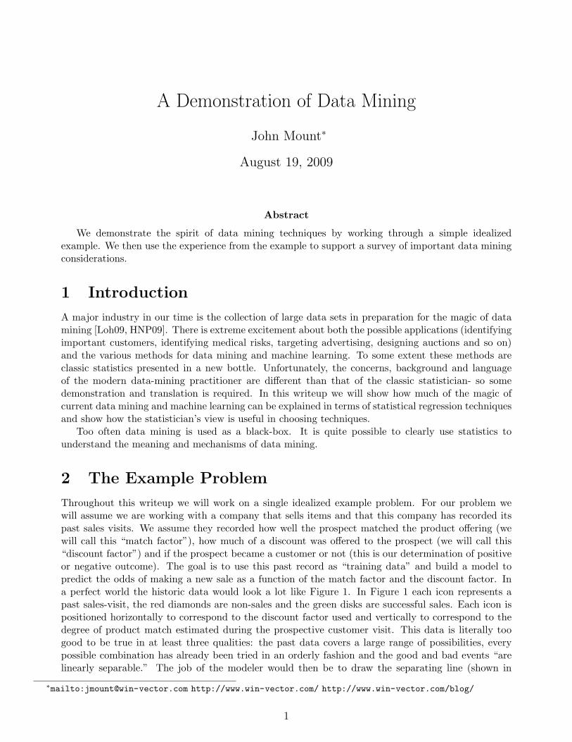
Throughout this writeup we will work on a single idealized example problem. For our problem wewill assume we are working with a company that sells items and that this company has recorded itspast sales visits. We assume they recorded how well the prospect matched the product offering (wewill call this “match factor”), how much of a discount was offered to the prospect (we will call this“discount factor”) and if the prospect became a customer or not (this is our determination of positiveor negative outcome). The goal is to use this past record as “training data” and build a model topredict the odds of making a new sale as a function of the match factor and the discount factor. Ina perfect world the historic data would look a lot like Figure 1. In Figure 1 each icon represents apast sales-visit, the red diamonds are non-sales and the green disks are successful sales. Each icon ispositioned horizontally to correspond to the discount factor used and vertically to correspond to thedegree of product match estimated during the prospective customer visit. This data is literally toogood to be true in at least three qualities: the past data covers a large range of possibilities, everypossible combination has already been tried in an orderly fashion and the good and bad events “arelinearly separable.” The job of the modeler would then be to draw the separating line (shown in
∗mailto:[email protected] http://www.win-vector.com/ http://www.win-vector.com/blog/
1
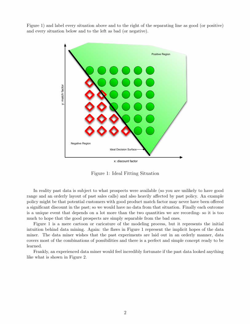
Figure 1) and label every situation above and to the right of the separating line as good (or positive)and every situation below and to the left as bad (or negative).
x: discount factor
y: m
atch
fact
or
Ideal Decision Surface
Positive Region
Negative Region
Figure 1: Ideal Fitting Situation
In reality past data is subject to what prospects were available (so you are unlikely to have goodrange and an orderly layout of past sales calls) and also heavily affected by past policy. An examplepolicy might be that potential customers with good product match factor may never have been offereda significant discount in the past; so we would have no data from that situation. Finally each outcomeis a unique event that depends on a lot more than the two quantities we are recording- so it is toomuch to hope that the good prospects are simply separable from the bad ones.
Figure 1 is a mere cartoon or caricature of the modeling process, but it represents the initialintuition behind data mining. Again: the flaws in Figure 1 represent the implicit hopes of the dataminer. The data miner wishes that the past experiments are laid out in an orderly manner, datacovers most of the combinations of possibilities and there is a perfect and simple concept ready to belearned.
Frankly, an experienced data miner would feel incredibly fortunate if the past data looked anythinglike what is shown in Figure 2.
2
x: discount factor
y: m
atch
fact
or
-2
0
2
4
-4 -2 0 2 4 6
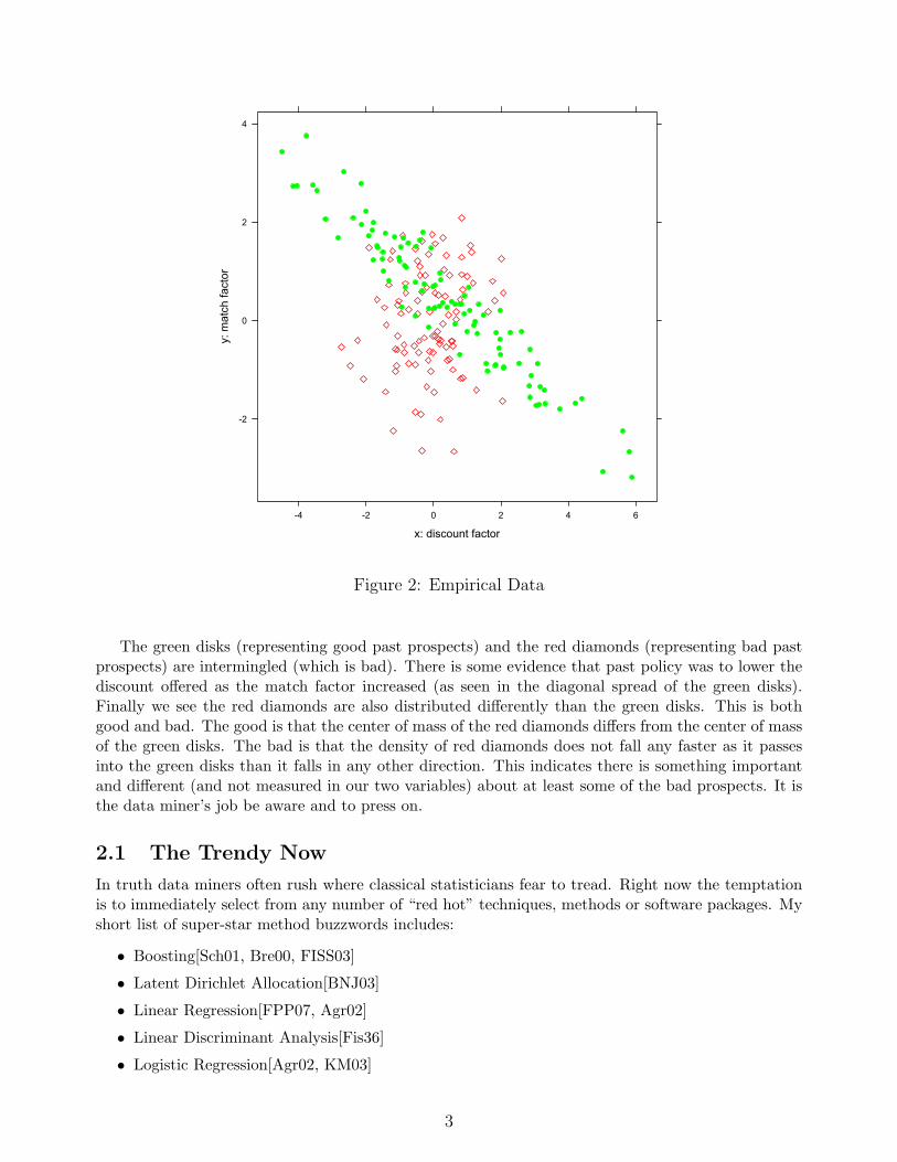
Figure 2: Empirical Data
The green disks (representing good past prospects) and the red diamonds (representing bad pastprospects) are intermingled (which is bad). There is some evidence that past policy was to lower thediscount offered as the match factor increased (as seen in the diagonal spread of the green disks).Finally we see the red diamonds are also distributed differently than the green disks. This is bothgood and bad. The good is that the center of mass of the red diamonds differs from the center of massof the green disks. The bad is that the density of red diamonds does not fall any faster as it passesinto the green disks than it falls in any other direction. This indicates there is something importantand different (and not measured in our two variables) about at least some of the bad prospects. It isthe data miner’s job be aware and to press on.
2.1 The Trendy Now
In truth data miners often rush where classical statisticians fear to tread. Right now the temptationis to immediately select from any number of “red hot” techniques, methods or software packages. Myshort list of super-star method buzzwords includes:
• Boosting[Sch01, Bre00, FISS03]
• Latent Dirichlet Allocation[BNJ03]
• Linear Regression[FPP07, Agr02]
• Linear Discriminant Analysis[Fis36]
• Logistic Regression[Agr02, KM03]
3
• Kernel Methods[CST00, STC04]
• Maximum Entropy[KM03, Gru05, SC89, DS06]
• Naive Bayes[Lew98]
• Perceptrons[BRS08, DKM05]
• Quantile Regression[Koe05]
• Ridge Regression[BF97]
• Support Vector Machines[CST00]
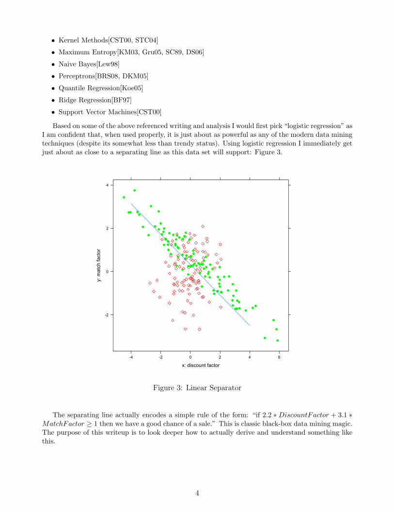
Based on some of the above referenced writing and analysis I would first pick “logistic regression” asI am confident that, when used properly, it is just about as powerful as any of the modern data miningtechniques (despite its somewhat less than trendy status). Using logistic regression I immediately getjust about as close to a separating line as this data set will support: Figure 3.
x: discount factor
y: m
atch
fact
or
-2
0
2
4
-4 -2 0 2 4 6
Figure 3: Linear Separator
The separating line actually encodes a simple rule of the form: “if 2.2 ∗ DiscountFactor + 3.1 ∗MatchFactor ≥ 1 then we have a good chance of a sale.” This is classic black-box data mining magic.The purpose of this writeup is to look deeper how to actually derive and understand something likethis.
4
3 Explanation
What is really going on? Why is our magic formula at all sensible advice, why did this work at all andwhat motivates the analysis? It turns out regression (be it linear regression or logistic regression) worksin this case because it somewhat imitates the methodology of linear discriminant analysis (describedin: [Fis36]). In fact in many cases it would be a better idea to perform a linear discriminant analysisor perform an analysis of variance than to immediately appeal to a complicated method. I will firststep through the process of linear discriminant analysis and then relate it to our logistic regression.Stepping through understandable stages lets us see where we were lucky in modeling and what limitsand opportunities for improvement we have.
x: discount factor
y: m
atch
fact
or
-2
0
2
4
-4 -2 0 2 4 6
Positive Example Points
x: discount factor
y: m
atch
fact
or
-2
-1
0
1
2
-2 -1 0 1 2
Negative Example Points
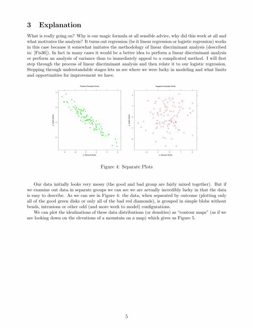
Figure 4: Separate Plots
Our data initially looks very messy (the good and bad group are fairly mixed together). But ifwe examine out data in separate groups we can see we are actually incredibly lucky in that the datais easy to describe. As we can see in Figure 4: the data, when separated by outcome (plotting onlyall of the good green disks or only all of the bad red diamonds), is grouped in simple blobs withoutbends, intrusions or other odd (and more work to model) configurations.
We can plot the idealizations of these data distributions (or densities) as “contour maps” (as if weare looking down on the elevations of a mountain on a map) which gives us Figure 5.
5

x: discount factor
y: m
atch
fact
or
-2
0
2
-2 0 2
0.05
0.10
0.15
0.200.25
0.30
-0.05
0.00
0.05
0.10
0.15
0.20
0.25
0.30
0.35
Distribution of Positive Examples
x: discount factor
y: m
atch
fact
or
-2
0
2
-2 0 2
0.050.100.150.200.250.30
-0.05
0.00
0.05
0.10
0.15
0.20
0.25
0.30
0.35
Distribution of Negative Examples
Figure 5: Separate Distributions
3.1 Full Bayes Model
From Figure 5 we can see while our data is not separable there are significant differences between thegroups. The difference in the groups is more obvious if we plot the difference of the densities on thesame graph as in Figure 6. Here we are visualizing the distribution of positive examples as a connectedpair of peaks (colored green) and the distribution of negative examples a deep valley (colored red)located just below and to the left of the peaks.
6

x: discount factor
y: m
atch
fact
or
-2
0
2
-2 0 2
-0.20
-0.15
-0.10
-0.05
0.00
0.05
0.10
0.15
0.20
Figure 6: Difference in Density
This difference graph is demonstrating how both of the densities or distributions (positive andnegative) reach into different regions of the plane. The white areas are where the difference in densitiesis very small which includes the areas in the corners (where there is little of either distribution) andthe area between the blobs (where there is a lot of mass from both distributions competing). Thisview is a bit closer to what a statistician wants to see- how the distributions of successes and failuresdifferent (this is a step to take before even guessing at or looking for causes and explanations).
Figure 6 is already an actionable model- we can predict the odds a new prospect will buy or notat a given discount by looking where they fall on Figure 6 and checking if they fall in a region onstrong red or strong green color. We can also recommend a discount for a given potential customer bydrawing a line at the height determined by their degree of match and tracing from left to right untilwe first hit a strong green region. We could hand out a simplified Figure 7 as a sales rulebook.
7

x: discount factor
y: m
atch
fact
or
-2
0
2
-2 0 2
Figure 7: Full Bayes Model
This model is a full Bayes model (but not a Naive Bayes model, which is oddly more famous andwhich we will cover later). The steps we took were: first we summarized or idealized our known datainto two Gaussian blobs (as depicted in Figure 5). Once we had estimated the centers, widths andorientations of these blobs we could then: for any new point say how likely the point is under themodeled distribution of sales and how likely the point is under the modeled distribution of non-sales.Mathematically we claim we can estimate P (x, y|sale)1 and P (x, y|non-sale) (where x is our discountfactor and y is our matching factor).2 Neither of these are what we are actually interested in (wewant: P (sale|x, y)3). We can, however, use these values to calculate what we want to know. Bayes’law is a law of probability that says if we know P (sale|x, y), P (non-sale|x, y), P (sale) and P (non-sale)4
then:P (sale|x, y) =
P (sale)P (x, y|sale)P (sale)P (x, y|sale) + P (non-sale)P (x, y|non-sale)
.
Figure 7 depicts a central hourglass shaped region (colored green) that represents the region of x, yvalues where P (sale|x, y) is estimated to be at least 0.5 and the remaining (darker red region) are the
1Read P (A|B) as: “the probability of A will happen given we know B is true.”2Technically we are working with densities, not probabilities, but we will use probability notation for its intuition.3P (sale|x, y) is the probability of making a sale as a function of what we know about the prospective customer and our
offer. Whereas P (x, y|sale) was just how likely it is to see a prospect with the given x and y values, conditioned on knowingwe made a sale to this prospect.
4 P (sale) and P (non-sale) are just the “prior odds” of sales or what our estimate of our chances of success are before welook at any facts about a particular customer. We can use our historical overall success and failure rates as estimates of thesequantities.
8

situations predicted to be less favorable. Here we are using priors of P (sale) = P (non-sale) = 0.5, fordifferent priors and thresholds we would get different graphs.
Even at this early stage in the analysis we have already accidentally introduced what we call “aninductive bias.” By modeling both distributions as Gaussians we have guaranteed that our acceptanceregion will be an hourglass figure (as we saw in Figure 7). One undesirable consequence of the modelingtechnique is the prediction sales become unlikely when both match factor and discount factor are verylarge. This is somewhat a consequence of our modeling technique (though the fact that the negativedata does not fall quickly as it passes into the green region also added to this). This un-realistic(or “not physically plausible”) prediction is called an artifact (of the technique and of the data) andit is the statistician’s job to see this, confirm they don’t want it and eliminate it (by deliberatelyintroducing a “useful modeling bias”).
3.2 Linear Discriminant
To get around the bad predictions of our model in the upper-right quadrant we “apply domainknowledge” and introduce a useful modeling bias as follows. Let us insist that our model be monotone:that if moving some direction is good than moving further in the same direction is better. In fact let’sinsist that our model be a half-plane (instead of two parabolas). We want a nice straight separatingcut, which brings us to linear discriminant analysis. We have enough information to apply Fisher lineardiscriminant technique and find a separator that maximizes the variance of data across categories whileminimizing the variance of data within one category and within the other category. This is called thelinear discriminant and it is shown in Figure 8.
x: discount factor
y: m
atch
fact
or
-2
0
2
-2 0 2
-0.20
-0.15
-0.10
-0.05
0.00
0.05
0.10
0.15
0.20
Figure 8: Linear Discriminant
9
The blue line is the linear discriminant (similar to the logistic regression line depicted earlier onthe data-slide). Everything above or to the right of the blue line is considered good and everythingbelow or to the left of the blue line is considered bad. Notice that this advice while not quite asaccurate as the Bayes Model near the boundary between the two distributions is much more sensibleabout the upper right corner of the graph.
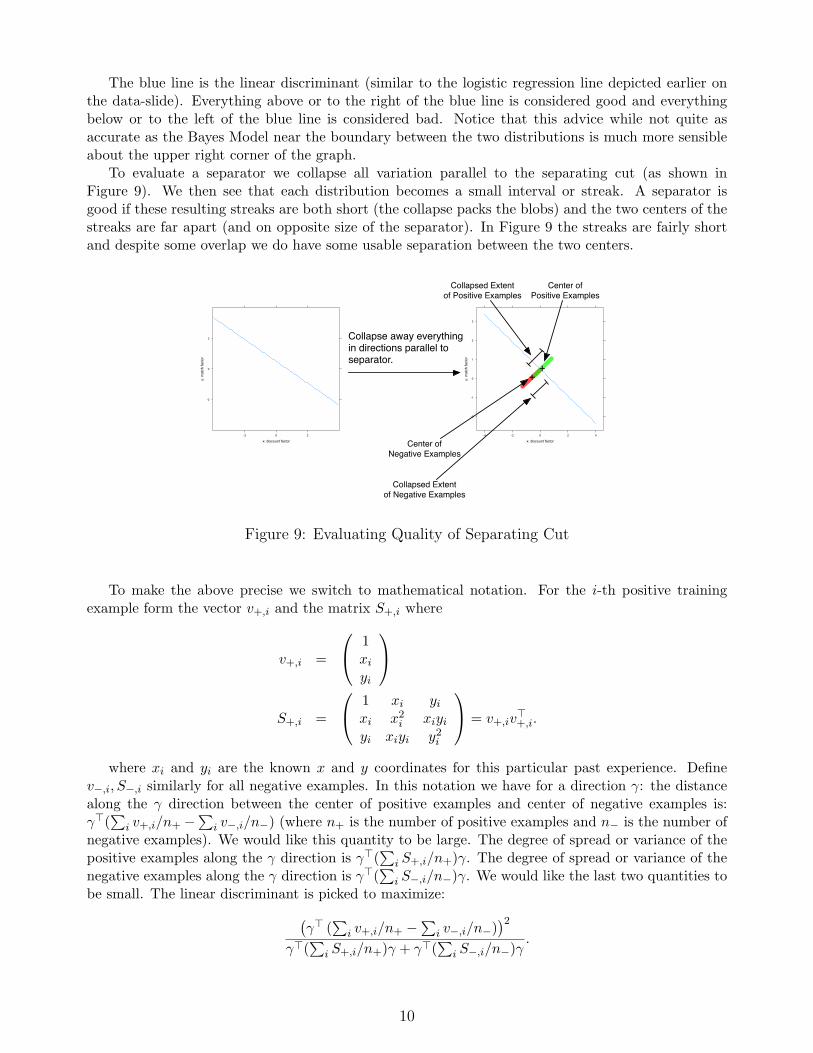
To evaluate a separator we collapse all variation parallel to the separating cut (as shown inFigure 9). We then see that each distribution becomes a small interval or streak. A separator isgood if these resulting streaks are both short (the collapse packs the blobs) and the two centers of thestreaks are far apart (and on opposite size of the separator). In Figure 9 the streaks are fairly shortand despite some overlap we do have some usable separation between the two centers.
x: discount factor
y: m
atc
h f
acto
r
-2
0
2
-2 0 2
Collapse away everythingin directions parallel toseparator.
x: discount factor
y: m
atc
h f
acto
r
-2
-1
0
1
2
3
-4 -2 0 2 4
Collapsed Extentof Positive Examples
Collapsed Extentof Negative Examples
++
Center ofNegative Examples
Center ofPositive Examples
Figure 9: Evaluating Quality of Separating Cut
To make the above precise we switch to mathematical notation. For the i-th positive trainingexample form the vector v+,i and the matrix S+,i where
v+,i =
1xi
yi
S+,i =
1 xi yi
xi x2i xiyi
yi xiyi y2i
= v+,iv>+,i.
where xi and yi are the known x and y coordinates for this particular past experience. Definev−,i, S−,i similarly for all negative examples. In this notation we have for a direction γ: the distancealong the γ direction between the center of positive examples and center of negative examples is:γ>(
∑i v+,i/n+ −
∑i v−,i/n−) (where n+ is the number of positive examples and n− is the number of
negative examples). We would like this quantity to be large. The degree of spread or variance of thepositive examples along the γ direction is γ>(
∑i S+,i/n+)γ. The degree of spread or variance of the
negative examples along the γ direction is γ>(∑
i S−,i/n−)γ. We would like the last two quantities tobe small. The linear discriminant is picked to maximize:(
γ> (∑
i v+,i/n+ −∑
i v−,i/n−))2
γ>(∑
i S+,i/n+)γ + γ>(∑
i S−,i/n−)γ.
10

It is a fairly standard observation (involving the Rayleigh quotient) that this form is maximized when:
γ =
(∑i
S+,i/n+ +∑
i
S−,i/n−
)−1(∑i
v+,i/n+ −∑
i
v−,i/n−
). (1)
As we have said, the linear discriminant is very similar to what is returned by a regression orlogistic regression. In fact in our diagrams the regression lines are almost identical to the lineardiscriminant. A large part of why regression can be usefully applied in classification comes from itsclose relationship to the linear discriminant.
3.3 Linear Regression
Linear regression is designed to model continuous functions subject to independent normal errors inobservation. Linear regression is incredibly powerful at characterizing and elimination correlationsbetween the input variables of a model. While function fitting is different than classification (ourexample problem) linear regression is so useful whenever there is any suspected correlation (which isalmost always the case) that it is an appropriate tool. In our example in the positive examples (thosethat led to sales) there is clearly a historical dependence between the degree of estimated match andamount of discount offered. Likely this dependence is from past prospects being subject to a (rational)policy of “the worse the match the higher the offered discount” (instead of being arranged in a perfectgrid-like experiment as in our first diagram: Figure 1). If this dependence is not dealt with we wouldunder-estimate the value of discount because we would think that discounted customers are not signingup at a higher rate (when these prospects are in fact clearly motivated by discount, once you controlfor the fact that many of the deeply discounted prospects had a much worse degree of match thanaverage).
For analysis of categorical data linear regression is closely linked to ANOVA (analysis ofvariance).[Agr02] Recall that variance was a major consideration with the linear discriminant analysis,so we should by now be on familiar ground.
In our notation the standard least-squares regression solution is:
β =
(∑i
S+,i +∑
i
S−,i
)−1(∑i
v+,iy+,i +∑
i
v−,iy−,i
)(2)
where y+,i = 1 for all i and y−,i = −1 for all i.If we have the same number of positive and negative examples (i.e. n+ = n−) then Equation 1
and Equation 2 are identical and we have β = γ. So in this special case the linear discriminantequals the least square linear regression solution. We can even ask how the solutions change if therelative proportions of positive and negative training data changes. The linear discriminant is carefullydesigned not to move, but the regression solution will tilt to be an angle that is more compatible withthe larger of the example classes and shift to cut less into that class. The linear regression solutioncan be fixed (by re-weighting the data) to also be insensitive to the relative proportions of positiveand negative examples but does not behave that way “fresh out of the box.”
3.4 Logistic Regression
While linear regression is designed to pick a function that minimizes the sum of square errors logisticregression is designed to pick a separator that maximizes something called the plausibility of the data.In our case since the data is so well behaved the logistic regression line is essentially the same as thelinear regression line. It is in fact an important property of logistic regression that there is always are-weighting (or choice of re-emphasis) of the data that causes some linear regression to pick the sameseparator as the logistic regression. Because linear and logistic regression are only identical in specific
11

circumstances it is the job of the statistician to know which of the two is more appropriate for a givendata set and given intended use of the resulting model.
4 Other Methods and Techniques
4.1 Kernelized Regression
One way to greatly expand the power of modeling methods is a trick called kernel methods. Roughlykernel methods are those methods that increase the power of machine learning by moving from asimple problem space (like ours in variables x and y) to a richer problem space that may be easierto work in. A lot of ink is spilled about how efficient the kernel methods are (they work in timeproportional to the size of the simple space, not the complex one) but this is not their essentialfeature. The essential feature is the expanded explanation power and this is so important that eventhe trivial kernel methods (such as directly adjoining additional combinations of variables) pick upmost of the power of the method. Kernel methods are also overly associated with Support VectorMachines- but are just as useful when added to Naive Bayes, linear regression or logistic regression.
For instance: Figure 10 shows a bow-tie like acceptance region found by using linear regressionover the variables x, y, x2, y2 and xy (instead of just x and y). Note how this result is similar to thefull Bayes model (but comes from a different feature set and fitting technique).
x: discount factor
y: m
atch
fact
or
-2
0
2
-2 0 2
x: discount factor
y: m
atch
fact
or
-2
0
2
-2 0 2
Figure 10: Kernelized Regression
12

4.2 Naive Bayes Model
We briefly return to the Bayes model to discuss a more common alternative called “NaiveBayes.” A Naive Bayes model is like a full Bayes model except an additional modelingsimplification is introduced in assuming that P (x, y|sale) = P (x|sale)P (y|sale) and P (x, y|non-sale) =P (x|non-sale)P (y|non-sale). That is we are assuming that the distributions of the x and ymeasurements are essentially independent (once we know which outcome happened). This assumptionis the opposite of what we do with regression in that we ignore dependencies in the data (instead ofmodeling and eliminating the dependencies). However, Naive Bayes methods are quite powerful andvery appropriate in sparse-data situations (such as text classification). The “naive” assumption thatthe input variables are independent greatly reduces the amount of data that needs to be tracked (it ismuch less work to track values of variables instead of simultaneous values of pairs of variables). Thecurved separator from this Naive Bayes model is illustrated in Figure 11.
x: discount factor
y: m
atch
fact
or
-2
0
2
-2 0 2
x: discount factor
y: m
atch
fact
or
-2
0
2
-2 0 2
Figure 11: Naive Bayes Model
The Naive Bayes version of the advice or policy chart is always going to be an axis-aligned parabolaas in Figure 12. Notice how both the linear discriminant and the Naive Bayes model make mistakes(places some colors on the wrong side of the curve)- but they are simple, reliable models that havethe desirable property of having connected prediction regions.
13

x: discount factor
y: m
atch
fact
or
-2
0
2
-2 0 2
Figure 12: Naive Bayes Decision
4.3 More Exotic Methods
Many of the hot buzzword machine learning and data mining methods we listed earlier are essentiallydifferent techniques of fitting a linear separator over data. These methods seem very different butthey all form a family once you realize many of the details of the methods are determined by:
• Choice of Loss FunctionThis is what notion of “goodness of fit” is being used. It can be normalized mean-variance (lineardiscriminants), un-normalized variance (linear regression), plausibility (logistic regression), L1distance (support vector machines, quantile regression), entropy (maximum entropy), probabilitymass and so on.
• Choice of Optimization TechniqueFor a given loss function we can optimize in many ways (though most authors make the mistakeof binding their current favorite optimization method deep into their specification of technique):EM, steepest descent, conjugate gradient, quasi-Newton, linear programming and quadraticprogramming to name a few.
• Choice of Regularization MethodRegularization is the idea of forcing the model to not pick extreme values of parameters toover-fit irrelevant artifacts in training data. Methods include MDL, controlling energy/entropy,Lagrange smoothing, shrinkage, bagging and early termination of optimization. Non-explicittreatment of regularization is one reason many methods completely specify their optimizationprocedure (to get some accidental regularization).
14

• Choice of Features/KernelizationThe richness of the feature set the method is applied to is the single largest determinant of modelquality.
• Pre-transformation TricksSome statistical methods are improved by pre-transforming the outcome data to look morenormal or be more homoscedastic.5
If you think along a few axes like these (instead of evaluating them by their name and lineage)you tend to see different data mining methods more as embodying different trade-offs than as beingunique incompatible disciplines.
5 Conclusion
Our goal for this writeup was to fully demonstrate a data mining method and then survey someimportant data mining and machine learning techniques. Many of the important considerations are“too obvious” to be discussed by statisticians and “too statistical” to be comfortably expressed interms popular with data miners. The theory and considerations from statistics when combinedwith the experience and optimism of data-mining/machine-learning truly make possible achievingthe important goal of “learning from data.”
This expository writeup is also meant to serve as an example of the types of research, analysis,software and training supplied by Win-Vector LLC http://www.win-vector.com . Win-Vector LLCprides itself in depth of research and specializes in identifying, documenting and implementing the“simplest technique that can possibly work” (which is often the most understandable, maintainable,robust and reliable). Win-Vector LLC specializes in research but has significant experience indelivering full solutions (including software solutions and integration with existing databases).
References
[Agr02] Alan Agresti, Categorical data analysis (wiley series in probability and statistics), Wiley-Interscience, July 2002.
[BF97] Leo Breiman and Jerome H Friedman, Predicting multivariate responses in multiple linearregression, Journal of the Royal Statistical Society, Series B (Methodological) 59 (1997),no. 1, 3–54.
[BNJ03] David M Blei, Andrew Y Ng, and Michael I Jordan, Latent dirichlet allocation, Journal ofMachine Learning Research 3 (2003), 993–1022.
[Bre00] Leo Breiman, Special invited paper. additive logistic regression: A statistical view of boosting:Discussion, Ann. Statist. 28 (2000), no. 2, 374–377.
[BRS08] Richard Beigel, Nick Reingold, and Daniel A Spielman, The perceptron strikes back, 6.
[CST00] Nello Cristianini and John Shawe-Taylor, An introduction to support vector machines andother kernel-based learning methods, 1 ed., Cambridge University Press, March 2000.
[DKM05] Sanjoy Dasgupta, Adam Tauman Kalai, and Claire Monteleoni, Analysis of perceptron-basedactive learning, CSAIL Tech. Report (2005), 16.
5A situation is homoscedastic if the errors are independent of where we are in the parameter space (our x,y or matchfactor and discount factor). This property is very important for meaningful fitting/modeling and interpreting significance offits.
15

[DS06] Miroslav Dudik and Robert E Schapire, Maximum entropy distribution estimation withgeneralized regularization, COLT (2006), 15.
[Fis36] Ronald A Fisher, The use of multiple measurements in taxonomic problems, Annals ofEugenics 7 (1936), 179–188.
[FISS03] Yoav Freund, Raj Iyer, Robert E Schapire, and Yoram Singer, An efficient boostingalgorithm for combining preferences, Journal of Machine Learning Research 4 (2003), 933–969.
[FPP07] David Freedman, Robert Pisani, and Roger Purves, Statistics 4th edition, W. W. Nortonand Company, 2007.
[Gru05] Peter D Grunwald, Maximum entropy and the glasses you are looking through.
[HNP09] Alon Halevy, Peter Norvig, and Fernando Pereira, The unreasonable effectiveness of data,IEEE Intellegent Systems (2009).
[KM03] Dan Klein and Christopher D Manning, Maxent models, conditional estimation, andoptimization.
[Koe05] Roger Koenker, Quantile regression, Cambridge University Press, May 2005.
[Lew98] David D Lewis, Naive (bayes) at forty: The independence assumption in informationretrieval.
[Loh09] Steve Lohr, For todays graduate, just one word: Statistics, http://www.nytimes.com/2009/08/06/technology/06stats.html, August 2009.
[Sar08] Deepayan Sarkar, Lattice: Multivariate data visualization with R, Springer, New York, 2008,ISBN 978-0-387-75968-5.
[SC89] Hal Stern and Thomas M Cover, Maximum entropy and the lottery, Journal of the AmericanStatistical Association 84 (1989), no. 408, 980–985.
[Sch01] Robert E Schapire, The boosting approach to machine learning an overview, 23.
[STC04] John Shawe-Taylor and Nello Cristianini, Kernel methods for pattern analysis, CambridgeUniversity Press, June 2004.
APPENDIX
A Graphs
The majority of the graphs in this writeup were produced using “R” http://www.r-project.org/and Deepayan Sarkar’s Lattice package[Sar08].
16