A delayed choice quantum eraser explained bythe transactional interpretation of quantum mechanics

H. Fearn

Physics Department, California State University Fullerton800 N. State College Blvd., Fullerton CA 92834

email: hfearn@fullerton.edu

Abstract

This paper explains the delayed choice quantum eraser of Kim et al. [1] in terms of the trans-actional interpretation of quantum mechanics by John Cramer [2, 3]. It is kept deliberatelymathematically simple to help explain the transactional technique. The emphasis is on a clearunderstanding of how the instantaneous “collapse” of the wave function due to a measurementat a specific time and place may be reinterpreted as a relativistically well-defined collapse overthe entire path of the photon and over the entire transit time from slit to detector. This ismade possible by the use of a retarded offer wave, which is thought to travel from the slits (orrather the small region within the parametric crystal where down-conversion takes place) to thedetector and an advanced counter wave traveling backward in time from the detector to the slits.The point here is to make clear how simple the transactional picture is and how much more intu-itive the collapse of the wave function becomes if viewed in this way. Also, any confusion aboutpossible retro-causal signaling is put to rest. A delayed choice quantum eraser does not requireany sort of backward in time communication. This paper makes the point that it is preferableto use the Transactional Interpretation (TI) over the usual Copenhagen Interpretation (CI) fora more intuitive understanding of the quantum eraser delayed choice experiment. Both methodsgive exactly the same end results and can be used interchangeably.

PACS codes: 03.65.Ta, 03.65.Ud, 42.50.Dv

Key Words: Transactional interpretation, advanced waves, delayed choice, quantum eraser

Complementarity, which path information and quantum erasers

Feynman 1965, in his famous lectures on physics [4] stated that the Young’s double slit experi-ment contains nearly all mysteries of quantum mechanics, namely, wave–particle duality, particletrajectories, collapse of the wave function and non locality. We may see interference, or we mayknow through which slit the photon passes, but we can never know both at the same time. Thisis what is commonly referred to as the principle of complementarity. We say two observables arecomplementary if precise knowledge of one implies that all possible outcomes of measuring theother are equally likely. The fundamental enforcement of complementarity arises from correla-tions between the detector and the interfering particle in a way that show up in the wave functionfor the system. It is not, as some undergraduate text books would have you believe, a consequenceof the uncertainty principle, although the application of the uncertainty principle makes for aneasy calculation when the wave function of the system is difficult to write out. There have beenmany gedanken (German for thought) experiments over the years to show complementarity. Themost famous are the Einstein recoiling slit, Feynman’s light scattering scheme both discussedin Feynman’s lectures on physics [4] and Wheeler’s delayed choice experiment [5]. The TI of

1

Figure 1: The figure shows the Scully Druhl quantum eraser 2 slit arrangement. Two 3-levelatoms are in place of the two slits. A laser excites either atom to the upper level a which maythen decay to level b or c. If the atom decays to level c, the ground state, then there will beinterference since there is no way to distinguish between the two atoms and so no which pathinformation. See figure (a). The green dots represent the single slit diffraction pattern. The solidline is the intensity detected. If the atom decays to level b, then there is which path informationand there will be no interference pattern as in figure (b). The drawings are simplified.

Cramer is preferred in this paper, over the usual CI, for a more intuitive understanding of thequantum eraser delayed choice experiment. An alternative theory, which also claims to presentan alternative perspective to the CI and provides an intuitive understanding of the paradoxes ofquantum mechanics, including the quantum eraser and delayed choice, is that by Sohrab [6, 7]which we mention for completeness, but will not discuss further there.Of particular interest here is the delayed choice quantum eraser gedanken experiment by Scullyand Druhl 1982 [8]. This work described a basic quantum eraser experiment and a delayed choicequantum eraser arrangement. The basic quantum eraser experiment is described using two 3-levelΛ–type atoms [9], in the place of two slits. See Fig. 1. The atoms start off in the ground stateand then a laser pulse comes in and excites either atom A or B. The excited atom then decaysand emits a signal photon. Interference fringes are sought between these signal photons on ascreen some distance away. Let the identical 3-level atoms have one upper level a and two lowerlevels b and c. The laser excites one of the atoms up to the level a but the atom can de-exciteto either state b or c. If both atoms start off in the ground state c, there are two possibilities.The excited atom decays and falls back to level c, so the excited atom becomes indistinguishablefrom the other atom which was not excited. In this case we would expect to see an interferencepattern since there is no which path information. In the second case, the excited atom drops tolevel b which is distinguishable from level c. In this case we have which path information and wewould get no interference pattern. That describes the basic quantum eraser.

For a delayed choice quantum eraser [8], the 3-level atoms change to 4-level atoms with levelsa, b, c, d, with d the ground state. See Fig. 2. Instead of one exciting laser pulse there are twoclosely spaced pulses, which will both go to the same atom. The first laser pulse excites eitheratom A or B from the ground state d to the upper level a. The excited atom then spontaneouslydecays to c emitting the signal photon. The second laser pulse then excites the atom from levelc to level b, which then decays with the emission of a lower energy idler photon to the groundstate. Now the atoms are inside a cleverly constructed cavity with a trap door separating them.The cavity is transparent to the signal photons and laser light but strongly reflects the idler

2

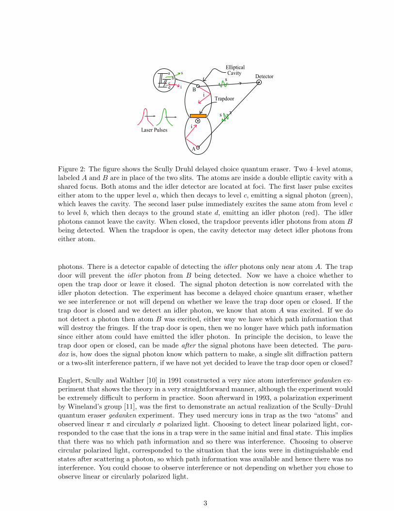
Figure 2: The figure shows the Scully Druhl delayed choice quantum eraser. Two 4–level atoms,labeled A and B are in place of the two slits. The atoms are inside a double elliptic cavity with ashared focus. Both atoms and the idler detector are located at foci. The first laser pulse exciteseither atom to the upper level a, which then decays to level c, emitting a signal photon (green),which leaves the cavity. The second laser pulse immediately excites the same atom from level cto level b, which then decays to the ground state d, emitting an idler photon (red). The idlerphotons cannot leave the cavity. When closed, the trapdoor prevents idler photons from atom Bbeing detected. When the trapdoor is open, the cavity detector may detect idler photons fromeither atom.

photons. There is a detector capable of detecting the idler photons only near atom A. The trapdoor will prevent the idler photon from B being detected. Now we have a choice whether toopen the trap door or leave it closed. The signal photon detection is now correlated with theidler photon detection. The experiment has become a delayed choice quantum eraser, whetherwe see interference or not will depend on whether we leave the trap door open or closed. If thetrap door is closed and we detect an idler photon, we know that atom A was excited. If we donot detect a photon then atom B was excited, either way we have which path information thatwill destroy the fringes. If the trap door is open, then we no longer have which path informationsince either atom could have emitted the idler photon. In principle the decision, to leave thetrap door open or closed, can be made after the signal photons have been detected. The para-dox is, how does the signal photon know which pattern to make, a single slit diffraction patternor a two-slit interference pattern, if we have not yet decided to leave the trap door open or closed?

Englert, Scully and Walther [10] in 1991 constructed a very nice atom interference gedanken ex-periment that shows the theory in a very straightforward manner, although the experiment wouldbe extremely difficult to perform in practice. Soon afterward in 1993, a polarization experimentby Wineland’s group [11], was the first to demonstrate an actual realization of the Scully–Druhlquantum eraser gedanken experiment. They used mercury ions in trap as the two “atoms” andobserved linear π and circularly σ polarized light. Choosing to detect linear polarized light, cor-responded to the case that the ions in a trap were in the same initial and final state. This impliesthat there was no which path information and so there was interference. Choosing to observecircular polarized light, corresponded to the situation that the ions were in distinguishable endstates after scattering a photon, so which path information was available and hence there was nointerference. You could choose to observe interference or not depending on whether you chose toobserve linear or circularly polarized light.

3

There have been many quantum optics experiments involving two photon entangled states andquantum eraser arrangements to demonstrate the complementarity arguments above. Three ofthe better ones are [12, 13, 14]. One experiment in particular by Zeilinger’s group [15] is worthyof a special note. The arm lengths in their apparatus were very long, between 55 m up to 144Km. They point out that there is no possible communication between one photon and the otherin the entangled pair because of the space-like separation between them and they assume nofaster-than-light communication is possible.

The most famous real experiment of the delayed choice type is that by Kim et al. [1], usingparametric down conversion entangled photons. It has drawn considerably more press thanany other experiment of this type and even has a couple of online animations [16]. We chooseto present our case for the transactional interpretation of quantum mechanics using the Kimexperiment as our example, but any of the delayed choice quantum erasers would work just aswell.

Introduction to the Transactional Interpretation of Quantum Mechanics

The transactional interpretation of quantum mechanics was proposed by John Cramer [2] in areview article in 1986 and a short overview in 1988 [17]. More recently Cramer has written abook [3] which should become available early in 2016. It is a way to view quantum mechanicsthat is very intuitive and easily accounts for all the well known quantum paradoxes, EinsteinRosen Podolsky (EPR ) experiment [18], which-way detection and quantum eraser experiments,[19, 20]. Unfortunately, it has garnered little support over the years and has fallen off the radar.It deserves a much broader dissemination and part of the motivation to publish this paper was tobring Cramer’s ideas, and the advanced wave concept, to the attention of the younger generationof physicists, who may not have heard of them before. The advanced wave is a standard solu-tion of relativistic wave equation and was utilized by such notable physicists as Dirac, Wheeler,Feynman, Davies, Hoyle and his doctoral student Narlikar. The direct particle interaction the-ory (which uses advanced waves, traveling backward in time) was used by Wheeler, Feynman,Schwinger, Hoyle and Narlikar. The direct particle interaction does away with the idea of afield, the vacuum field then would be truly empty, with zero energy, as Feynman believed. FrankWilczek recounts a conversation with Feynman [21].

Around 1982, I had a memorable conversation with Feynman at Santa Barbara.Usually, at least with people he didn’t know well, Feynman was “on” – in performancemode. But after a day of bravura performances he was a little tired and easedup. Alone for a couple of hours, before dinner, we had a wide-ranging discussionabout physics. Our conversation inevitably drifted to the most mysterious aspect ofour model of the world– both in 1982 and today– the subject of the cosmologicalconstant. (The cosmological constant is, essentially, the energy density of emptyspace. Anticipating a little, let me just mention that a big puzzle in modern physicsis why empty space weighs so little even though there’s so much to it.) I askedFeynman, “Doesn’t it bother you that gravity seems to ignore all we have learnedabout the complications of the vacuum?” To which he immediately responded, “Ionce thought I’d solved that one.” Then Feynman became wistful. Ordinarily hewould look you right in the eye, and speak slowly but beautifully, in a smooth flowof fully formed sentences or even paragraphs. Now, however, he gazed off into space;

4

he seemed transported for a moment, and said nothing. Gathering himself again,Feynman explained that he had been disappointed with the outcome of his workon quantum electrodynamics. It was a startling thing for him to say, because thatbrilliant work was what brought Feynman graphs to the world, as well as many ofthe methods we still use to do difficult calculations in quantum field theory. It wasalso the work for which he won the Nobel Prize. Feynman told me that when herealized that his theory of photons and electrons is mathematically equivalent to theusual theory, it crushed his deepest hopes. He had hoped that by formulating histheory directly in terms of paths of particles in space–time – Feynman graphs – hewould avoid the field concept and construct something essentially new. For a whilehe thought he had. Why did he want to get rid of fields? “I had a slogan,” he said.Ratcheting up the volume and his Brooklyn accent, he intoned it:

The vacuum doesn’t weigh anything [dramatic pause] because there’s nothing there!

Experimental observations show that the vacuum energy density is in fact very close to zero. Tocalculate the vacuum energy in quantum field theory, we must admit that spacetime is probablynot a continuum but rather has a discrete nature, at quantum dimensions, and only sum thezero-point energies for vibrational modes having wavelengths larger than, the Planck length (10−35 m) and less than or equal to the size of the universe (diameter approx. 8.8× 1026m). Thisgives a ridiculously large but finite vacuum energy density of about 10111 Jm−3 or in terms ofmass density 1094 Kgm−3. Clearly, no where near the experimentally observed value for energydensity near zero and mass density, near the critical value of 10−26 Kgm−3. The quantum fieldtheory vacuum mass density is about 120 orders of magnitude too large – rather embarrassingreally.

Absorber theory and Advanced Waves and Direct Particle Interaction Theory

The idea of advanced waves in classical electrodynamics started with Dirac [22] in 1938 and hisderivation of the radiation reaction of a charged accelerated particle. Advanced waves travelbackward in time and are a perfect way to allow for action-at-a-distance. A remote particle caninteract with a local source particle by absorbing retarded waves from the source in the futureand in response, emits an advanced wave which travels backward in time and interacts withthe source immediately, at the instant the retarded wave was emitted. This is a direct particleinteraction and does not require the presence of a field. This direct particle interaction conservesmomentum. Dirac assumed an advanced wave, in his radiation reaction calculations, but gave nophysical explanation as to where it came from. Later Wheeler and Feynman [23] wrote papersin 1945 and 1949 on absorber theory, which was their attempt to give a physical description ofthe origins of the advanced waves introduced by Dirac. An added motivation was to try andremove the self energy from the electron, but that was not entirely successful, as Wilzcek re-counts above. The radiation reaction could be accounted for without self interaction, but at thequantum level self-interaction became unavoidable for charge renormalization, electron –positronpairs are still required to shield the infinite negative bare mass. With an upper bound (Rindlerhorizon caused by an accelerating expansion ) and lower length cutoff (Schwarzschild radius of aparticle about 10−45cm) , the standard renormalization procedure can be applied to the directparticle interaction approach, which is then no less suitable than conventional field theory, buthas no cosmological constant problem. There are no classical divergences if the self-interactionis non-quantized. Feynman’s PhD thesis included the path integral approach to non-relativisticquantum mechanics, which was used to describe how to quantize the direct particle interaction

5

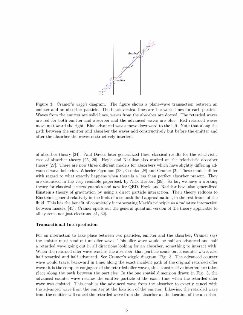
Figure 3: Cramer’s wiggle diagram. The figure shows a plane-wave transaction between anemitter and an absorber particle. The black vertical lines are the world-lines for each particle.Waves from the emitter are solid lines, waves from the absorber are dotted. The retarded wavesare red for both emitter and absorber and the advanced waves are blue. Red retarded wavesmove up toward the right. Blue advanced waves move downward to the left. Note that along thepath between the emitter and absorber the waves add constructively but before the emitter andafter the absorber the waves destructively interfere.

of absorber theory [24]. Paul Davies later generalized these classical results for the relativisticcase of absorber theory [25, 26]. Hoyle and Narlikar also worked on the relativistic absorbertheory [27]. There are now three different models for absorbers which have slightly differing ad-vanced wave behavior. Wheeler-Feynman [23], Csonka [28] and Cramer [2]. These models differwith regard to what exactly happens when there is a less than perfect absorber present. Theyare discussed in the very readable paperback by Nick Herbert [29]. So far, we have a workingtheory for classical electrodynamics and now for QED. Hoyle and Narlikar have also generalizedEinstein’s theory of gravitation by using a direct particle interaction. Their theory reduces toEinstein’s general relativity in the limit of a smooth fluid approximation, in the rest frame of thefluid. This has the benefit of completely incorporating Mach’s principle as a radiative interactionbetween masses, [45]. Cramer spells out the general quantum version of the theory applicable toall systems not just electrons [31, 32].

Transactional Interpretation

For an interaction to take place between two particles, emitter and the absorber, Cramer saysthe emitter must send out an offer wave. This offer wave would be half an advanced and halfa retarded wave going out in all directions looking for an absorber, something to interact with.When the retarded offer wave reaches the absorber, that particle sends out a counter wave, alsohalf retarded and half advanced. See Cramer’s wiggle diagram, Fig. 3. The advanced counterwave would travel backward in time, along the exact incident path of the original retarded offerwave (it is the complex conjugate of the retarded offer wave), thus constructive interference takesplace along the path between the particles. In the one spatial dimension drawn in Fig. 3, theadvanced counter wave reaches the emitter particle at the exact time when the retarded offerwave was emitted. This enables the advanced wave from the absorber to exactly cancel withthe advanced wave from the emitter at the location of the emitter. Likewise, the retarded wavefrom the emitter will cancel the retarded wave from the absorber at the location of the absorber.

6

Only the retarded wave from the emitter and the advanced wave from the absorber along theadjoining path are enhanced by the superposition, they do not cancel out. These waves representthe interaction between the particles.

In three spatial dimensions things are a little more complicated. Advanced and retarded wavestravel in all directions not just in the direction of one absorber. Retarded waves carry on intothe future and maybe absorbed at some later point in time. An advanced wave travels backwardin time to the big bang. At this point it is reflected and will move forward in time as an advancedwave identical to, and π out of phase with, the incident advanced wave. This will produce acancellation at every point along the world-line back to the point of emission of the wave. Alladvanced waves therefore cancel out, [30]. Note that the waves are assumed to travel at speedc the speed-of-light in a vacuum, although the advanced wave is traveling backward in time,or with -t [31]. Basically, in quantum terms, the regular wave function is the offer wave, (orat least the retarded wave part that does not cancel out) the complex conjugate wave functionis the confirmation wave (the advanced part moving between the absorber going back in timeto the emitter) and together they give a handshake [32], which allows an interaction to take place.

Recently Kastner [33] has expounded the virtues of the transactional method with an additionaltwist allowing for free will. There are many examples of the use of the transactional method inthe book and it is well worth a read. In this paper we make no distinction between the originalCramer Transactional Interpretation (TI) and the Kastner version of Possibilist TransactionInterpretation (PTI). Kastner’s approach [34],

“is to consider a growing emergent universe in which the future is not set in stonebut is actualized from an underlying substratum of quantum possibilities.”

Cramer’s approach means (from the authors view point) that the future is set, the past, presentand future may all coexist and we simply have the illusion of flowing through time. To avoidconfusion, we quote Cramer on his own interpretation [35];

“Let me give an example. When you use your cash card at the grocery store to payfor your purchases, the electronic handshake that occurs between the bank and thecash register insures that money is “conserved” and is neither created nor destroyed,but it does not determine what you elected to purchase. The same is true withquantum transactions, which guarantee the conservation laws but do not determinethe future. The real difference between Kastner’s PTI and my TI is that for her,offer and confirmation waves exist as objects only in some multidimensional Hilbertspace. In the TI the waves exist in real 3+1 dimensional space. Hilbert space wasinvented by theorists prone to abstraction because it was the only way they couldimagine that quantum waves could be entangled. The TI explains how they canbe entangled, because the multi-particle transactions allow only those subset of thewaves that satisfy the conservation laws to become real transactions.”

Others have considered a Many-Worlds Interpretation, with every possible event happening alongparallel realities in order to maintain free will. Neither Kastner nor Cramer agree with the many-worlds view [18]. Here, the reader is asked to make up their own mind. This paper is concernedonly with; Does the transactional interpretation fit the data or not? It is found that all the usualquantum results hold and the TI is simply an alternative point of view from the Copenhageninterpretation, and the instantaneously collapsing wave function, way of thinking.

7

The delayed choice quantum eraser by Kim et al.

First we briefly explain the experiment and the observed results. The experimental arrangementcan be seen in Fig. 4. An argon laser ( λp = 351.1 nm) is passed through a double slit andilluminates a type II phase matching nonlinear crystal of β- Barium Borate BBO (β −BaB2O4)The slit A allows region A of the crystal to be illuminated and slit B allows only region B of thecrystal to be illuminated. This small region is about 0.3 mm long which we take to be the slitwidth a. The separation d of the two regions is about 0.7 mm as specified in the paper [1]. So wemay discuss regions A and B of the crystal just as well as the original 2 slits. Parametric downconversion will occur at both sites and from the one pump photon will emerge two photons, asignal and an idler. Note that all possible frequencies are created νp = νs + νi. We are selectingtwo of the same frequency, or equivalently, twice the pump wavelength λs = 702.2 nm. Thesignal and idler photons represent the e-ray and o-ray of the nonlinear crystal.

These photons are momentum entangled and are created essentially at the same time. The prob-ability for a downconversion event is slight, so we may assume that there is only one entangledpair of photons in the system at any given time. Different wavelengths of signal and idler photonsexit the crystal at different angles. The required wavelengths are selected by restricting the exitangle. Usually a small range of wavelengths would be selected. For convenience we track onlyone wavelength, but we should bear in mind that there will be a small bandwidth of wavelengthswhich will affect the interference pattern of the signal photons and change the visibility of thefringes accordingly. The bandwidth can also be changed using filters in front of the detectors.The detectors will have a less than perfect efficiency which will also affect the fringe visibility.The efficiency of the detectors was not mentioned in the experiment however, and neither wasthe effective bandwidth.

The signal photons are sent though a lens, of focal length f , (not specified in the paper [1]) andthen focussed onto a screen where they can be detected by detector D0. The detector scans, viastepper motor, along the x-axis to build up a pattern. The lens is used to create the far field condi-tion at the detector so we expect a Fraunhofer type pattern which is built up over time. The idlerphotons, from region A and B of the crystal, are sent in the direction of a Glen-Thompson prism(a wedge mirror is used in figure 4. instead) which separates them into different paths. The idlerphotons from region A hit BSA and are either reflected or transmitted. The reflected photonswill be detected by D3. The transmitted photons will be reflected by mirror MA and then eithertransmitted through the beamsplitter BS to detector D2 or reflected by BS into detector D1.The idler photons from B hit BSB and are either reflected or transmitted. The reflected photonswill be detected by D4. The transmitted photons will be reflected by mirror MB and then ei-ther transmitted through the beamsplitter BS to detector D1 or reflected by BS into detector D2.

The time of flight from the crystal to the detector D0 for the signal photons is 8 ns shorter thanfor the idler photons which go in the direction of the beamsplitters and were eventually detectedby detectors D3, D4 or by D1 or D2. The equivalent path length is approximately 2.5 m. Weassume that all the detector path lengths, D1 – D4, are the same and equal to 2.5 m. This pathlength will introduce a constant phase shift into each joint detection. It is also assumed that allmirror reflection angles are the same in both paths so that no additional phase shift differencesneed to be considered. Since all the phase shifts are considered equal they will cancel out andwill not effect the overall interference pattern.

All the detectors are linked to a coincidence counter and the interference patterns are recorded.

8

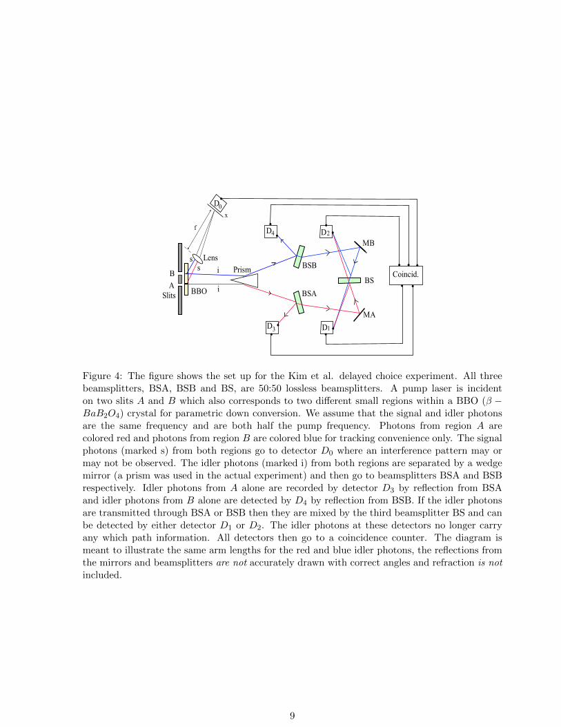
Figure 4: The figure shows the set up for the Kim et al. delayed choice experiment. All threebeamsplitters, BSA, BSB and BS, are 50:50 lossless beamsplitters. A pump laser is incidenton two slits A and B which also corresponds to two different small regions within a BBO (β −BaB2O4) crystal for parametric down conversion. We assume that the signal and idler photonsare the same frequency and are both half the pump frequency. Photons from region A arecolored red and photons from region B are colored blue for tracking convenience only. The signalphotons (marked s) from both regions go to detector D0 where an interference pattern may ormay not be observed. The idler photons (marked i) from both regions are separated by a wedgemirror (a prism was used in the actual experiment) and then go to beamsplitters BSA and BSBrespectively. Idler photons from A alone are recorded by detector D3 by reflection from BSAand idler photons from B alone are detected by D4 by reflection from BSB. If the idler photonsare transmitted through BSA or BSB then they are mixed by the third beamsplitter BS and canbe detected by either detector D1 or D2. The idler photons at these detectors no longer carryany which path information. All detectors then go to a coincidence counter. The diagram ismeant to illustrate the same arm lengths for the red and blue idler photons, the reflections fromthe mirrors and beamsplitters are not accurately drawn with correct angles and refraction is notincluded.

9

The intensity pattern recorded at D0 shows no interference when there is a coincidence betweenD0 and D3 or D4. In these cases, we have which path information, since D3 only records idlerphotons from slit A and D4 only records idler photons from slit B. Since the signal and idlerphotons come from the same region of the crystal, we would then know through which path thesignal photons came and we expect no interference.

When the coincidence counts are between D0 and D1 there is an interference pattern. Thebeamsplitter BS mixes the idler photons from both regions and we have now erased the whichpath information. There is also an interference pattern when there is a coincidence between D0

and D2 but this pattern differs from the previous one by a phase shift of π. In other words ifone pattern shows a co-sinusoidal interference the other will be sinusoidal. The experiment isconsidered a delayed choice quantum eraser since the signal photons path length is shorter thanthe idler photons. It would seem that the signal photons are detected first, then we make aselection of which coincidence detections to look at, and depending on that choice we see or donot see interference of the signal photons. The paradox being, how can you influence the signalphoton, basically tell it to interfere or not, by making a choice of detector D1 −D4,8 ns after the signal photon has already been detected by D0. This however is the wrong way tothink about this problem. If looked at in the correct way there is no paradox.

These observations can easily be explained in terms of the transactional interpretation of quantummechanics as follows. A brief account of this experiment is given in the book by Kastner [33], wegive a bit more detail here.

Transactional interpretation derivation

Let us start with a few preliminaries. The three beamsplitters in the experiment are all 50:50lossless beamsplitters. When a photon wavepacket goes through one of these beamsplitters thereis no loss so one would expect the probability amplitude of the wave function to remain unaltered.

|ψ|2 = |rψ + tψ|2

= [|r|2 + |t|2 + (r∗t+ rt∗)]|ψ|2 (1)

This means that the amplitude reflection and transmission coefficients obey,

|r|2 + |t|2 = 1

|r|2 = |t|2 =1

2r∗t+ rt∗ = 0

hence r =i√2

and t =1√2. (2)

We take all the beamsplitters to be identical for convenience. It will be assumed that each opticalpath length for the idler photons, is the same and any phase changes due to mirror reflectionshave been compensated for. An offer wave will go out from the slits and get absorbed by a de-tector. The detector will then send back an advanced wave (backwards in time) along the samepath as the incident wave to the slits to handshake and confirm the interaction. Only then doesthe photon actually leave the slit region. The offer wave is a momentum entangled two-photonstate (or bi-photon). The possible transactions will depend on the detector configuration whichgenerates the counter wave. We will go through the process step by step.

10

The original offer wave from the slits comes from the pump laser beam, we will take this to be,

ψ =α√2

(|Ap〉+ |Bp〉) (3)

where the subscript p stands for pump. The α is the single slit diffraction pattern, a sinc functionof the usual kind. A and B stand for the photon wave functions from the two slits, of plane wavetype. Parametric downconversion inside the β-barium borate (BBO) crystal duplicates eachpump photon into a signal and an idler photon. For type I parametric down conversion, thesignal and idler have the same polarization, for type II the signal and idler polarizations areperpendicular. This is of no importance here since the signal photons from regions A and Binterfere at detector D0 and both idler photons interfere at one of the four detectors D1–D4. Theoffer wave from the 2 slits and crystal then becomes,

ψ =α√2

(|As〉|Ai〉+ |Bs〉|Bi〉) . (4)

We select both the signal and idler photons of half the pump frequency, by restricting the exitangle from the crystal. Even so there will be a small spread in frequency, and thus wavelength,which will cause the fringe visibility to be less than perfect. However, we will continue thinkingof the photons wave functions as simple monochromatic plane waves for simplicity. It is easy togeneralize the end result for more than one wavelength.

The time dependent, correlation function calculation can be found in Appendix A. This isfor comparison with the TI approach taken below. We skip the details of the parametric down-conversion process in what follows, but they can be found in [36, 37, 38, 9] and these results areused in the Appendix A calculation. The first reference refers to 5 basic quantum experimentsand has simple theory accessible to undergraduates [36]. The second reference has more theorybut still some experiment, and is geared more for graduates and researchers [37] and the last tworeference is a theory paper and a text book [38, 9].

The signal photons are sent to the detector D0. The idler photons are sent to the beamsplittersetup. The path lengths in the experiment are arranged so that the signal photons reach detectorD0 before the idler photons reach their final destination. So if the signal photon is detected atposition x on the screen, then our offer wave becomes [33]

ψ =α√2

(〈x|As〉|Ai〉+ 〈x|Bs〉|Bi〉) . (5)

A simple fourier transform of a slit with a constant electric field will give the single slit diffractionamplitude α in the form

α = sinc(kxa/2) (6)

where a is the slit width and kx = k sin θ and the angle θ is the angular displacement from thecenter of the slits to the position x on the screen. For the paraxial ray approximation this wouldbe

kx = k sin θ =kx

f=πx

λf(7)

where f is the focal length of the lens which is taken to be roughly the slit screen distance andλ is the wavelength of the signal photons and we have used k = 2π/λ. Hence

α = sinc

(kxa

2f

)= sinc

(πxa

λf

)(8)

11

We will now assume that

〈x|As〉 = eikxdA

〈x|Bs〉 = eikxdB (9)

where dA and dB are the distances from the crystal regions A and B to the screen at position x.Also we assume that the slit separation can be given by d = dA − dB. The offer wave can nowbe written as,

ψow =α√2

(eikxdA |Ai〉+ eikxdB |Bi〉

). (10)

Note that we have now dealt with the signal photons and only have to concern ourselves with theidler photon detection. At this point we can continue with the Cramer interpretation or take thewave function Eq. (10) as a standard wave function and use spontaneous emission photon wavepackets and expand them in terms or retarded and advanced waves to clearly see the overlap ofthe two and how the advanced waves retrace the retarded wave in time. This is carried out, forCase 1. below, in Appendix B. to show the technique. Three cases follow:

Case 1:

Assume the idler photon will be detected at detector D1. The offer wave produced by passingphotons through the beamsplitters will be

ψow =α√2

(eikxdAtr|Ai〉+ eikxdB t2|Bi〉

)(11)

the Ai idler photon is transmitted through BSA and reflected from BS to reach D1. The Biidler photon is transmitted through BSB and transmitted through BS to reach D1. See Fig. 4for details of the paths. We have assumed that the extra path length in traveling through thebeamsplitters is the same for both photons Ai and Bi, otherwise we would need additional phasefactors to account for the path length difference. The counter wave produced by detector D1 willbe the complex conjugate wave traveling backward in time towards the slits,

ψ∗cw =α∗√

2

(e−ikxdAt∗r∗〈Ai|+ e−ikxdB t∗2〈Bi|

). (12)

The probability that this transaction will occur then becomes,

ψ∗cwψow =1

2|α|2

[|r|2|t|2〈Ai|Ai〉+ |t|4〈Bi|Bi〉+ |t|2

(r∗t〈Ai|Bi〉e−ikxd + rt〈Bi|Ai〉eikxd

)](13)

Let the amplitudes 〈Ai|Ai〉 = 〈Bi|Bi〉 = 1, 〈Ai|Bi〉 = η1/21 exp(−iφ) and complex conjugate

〈Bi|Ai〉 = η1/21 exp(iφ) , where η1 represents the detector efficiency of D1 which is most likely

less than unity. The detector efficiency has been incorporated into the probability amplitude forconvenience only. Then we may write,

ψ∗cwψow =1

2|α|2|t|2

[(|r|2 + |t|2) + η1

(r∗te−i(kxd+φ) + rtei(kxd+φ)

)]. (14)

Using our earlier results Eq(2) for the amplitudes r and t of the lossless beamsplitters and

e±iπ/2 = cosπ/2± i sinπ/2 = ±i (15)

12

we get,

ψ∗cwψow =1

4|α|2 [1 + η1 cos(kxd+ φ+ π/2)]

=1

4|α|2

[1 + η1 cos

(πd

λf+ φ+ π/2

)](16)

It is more general to leave the result in this form. However the Kim paper [1] goes on to simplifyfurther, uses η1 = 1 for perfect detection and writes,

ψ∗cwψow =1

2|α|2 cos2

[kxd

2+φ

2+π

4

](17)

where α is given by Eq.(8) and kx is given by Eq.(7). In the last step we used the double angleformula for cos 2β = 2 cos2 β − 1. This is the coincidence result between detector D1 togetherwith detector D0 and shows interference.

Using our result Eq.(16) it is easy to generalize to a small spread of wavelengths (bandwidth=∆λ)by using a computer code to plot the equation and summing the interference patterns for λ,λ±∆λ, λ±∆λ/2 and λ±∆λ/4. This will give a quite accurate interference pattern which willmatch the experimental data very well. If you also include the detector efficiency η1 then youcan match the experimental fringe visibility almost exactly. This is easy to do with a symbolicmanipulation code like Mathematica, which also plots the results for you.

Case 2:

When the idler photons are detected at D2 the offer wave becomes,

ψow =α√2

(eikxdAt2|Ai〉+ eikxdB tr|Bi〉

)(18)

Note that the Ai photon is transmitted by both BSA and BS, and the Bi photon is transmittedby BSB but reflected by BS to reach D2. See Fig. 4 for details. The detector produces a counterwave which is the complex conjugate of the offer wave above,

ψ∗cw =α∗√

2

(e−ikxdAt∗2〈Ai|+ e−ikxdB t∗r∗〈Bi|

)(19)

Using the same manipulations as before, leaving the detector efficiency as unity, the joint prob-ability detection of coincidence counts between D0 and D2 becomes,

ψ∗cwψow =|α|2

2|t|2[|t|2〈Ai|Ai〉+ |r|2〈Bi|Bi〉+

(t∗r〈Ai|Bi〉e−ikxd + r∗t〈Bi|Ai〉eikxd

)]=|α|2

4

[1 +

i

2e−i(kxd+φ) − i

2ei(kxd+φ)

]=|α|2

4

[1 + cos

(kxd+ φ− π

2

)]=|α|2

2cos2

(kxd

2+φ

2− π

4

)(20)

which also shows interference. The factor α is given by Eq.(8). Note that this interference isπ out of phase with the interference pattern obtained from the coincidence count between D0

13

and D1. This is easier to see in the cosine result rather than the cos2 result. That means if theinterference with D1 is co-sinusoidal then this interference would be sinusoidal. This is exactlywhat was observed in the experiment [1].

Case 3:

If the idler photon is detected at either D3 or D4 then the corresponding offer waves would be,

ψow =αr√

2

(eikxdA |Ai〉+ eikxdB |Bi〉

)(21)

and the counter waves would be

ψ∗cw3 =α∗r∗√

2〈Ai|e−ikxdA for detector D3

ψ∗cw4 =α∗r∗√

2〈Bi|e−ikxdB for detector D4 (22)

The probability of a coincidence count between D0 and D3 becomes,

ψ∗cw3ψow =|α|2|r|2

2〈Ai|Ai〉 =

|α|2

4(23)

which shows no interference only a single slit diffraction pattern. The probability of a coincidencecount between D0 and D4 becomes,

ψ∗cw4ψow =|α|2|r|2

2〈Bi|Bi〉 =

|α|2

4(24)

which likewise shows no interference. Again, the single slit diffraction amplitude α is given byEq ( 8). This also agrees with the experimental results of Kim et al. [1].

Discussion

The transactional interpretation is related to the direct particle interaction theory of Wheeler –Feynman and Hoyle – Narlikar and involves advanced waves as well as the usual retarded waves.The advanced waves are natural solutions to the relativistic wave equation and are required toconserve momentum in direct particle interactions. This paper has briefly considered the prosand cons of direct particle interactions verse conventional field theory methods. In terms ofvacuum energy density the direct particle approach tells us there is no vacuum field and thusits energy is identically zero, close in fact to the observed value. Quantum field theory tells usthat the vacuum energy density is huge and gives a value 120 times too large. Direct particle orsource theory does away with self interaction and subtracting infinities is only needed for chargerenormalization. Charge renormalization follows in the same manner as in the field theory casewhen you introduce a size cutoff (no point particles) of the Schwarzschild radius of the particle.There is also a size limit to the universe to prevent a divergent advanced wave integral due to theRindler horizon for an accelerating expansion of the universe [39]. Advanced waves have neverbeen detected in practice and this lack of experimental evidence is enough for some to rule themout altogether.

It only takes one experimental observation to refute a theory. John Cramer and Nick Herbert[40] considered several experimental possibilities of nonlocal quantum signaling (retrocausal sig-nals) involving path entangled systems and in all cases found that the complementarity between

14

two-photon interference and one-photon interference blocks any potential nonlocal signal [41].The traditional way of thinking about an instantaneous wave function collapse, at a certain timeat a certain place, which is clearly in conflict with relativity, is superseded in the transactionalpicture. The wave function collapse is among the most confusing aspects of quantum mechanics(as a component of the measurement problem) and is simply resolved using the TI method ofCramer, or PTI of Kastner. Indeed the Copenhagen approach actually evades the entire issueby taking the wave function and its collapse as epistemic–a measure of knowledge rather thana physical entity. This approach is observer-dependent; it is subject to the ’Heisenberg Cut’in which there is no physically grounded and non-arbitrary account of what constitutes an ’ob-server’. In the transactional approach, there is no observer-dependence: it is absorbers thatprovide the missing ingredient that defines when a measurement and attendant collapse occurs.

Advanced waves are natural solutions to relativistic wave equations. In order to use this theoryfor the nonrelativistic case it is necessary to think of two Schrodinger equations: one Schrodingerequation for the wave function ψ and one for its complex conjugate ψ∗, which becomes the ad-vanced wave. This makes sense if we think of the Schrodinger equation as a square root versionof the relativistic Klein Gordon equation.

Furthermore, work by Hogarth [42] and Hoyle and Narlikar (HN) [43, 44, 45] has paved theway to a new version of direct particle interaction gravitational theory, which is fully Machian,incorporates advanced waves and has Einstein’s theory as a special case. The HN theory may bequantized as in their book [45] using the path integral technique pioneered by Feynman [24].

It is interesting to note that the mass field m(x) in HN theory looks similar to the sourcefield S(x) introduced by Schwinger [46]. Wheeler never gave up on the absorber theory, whichis a direct particle interaction (action–at–a–distance) theory. It simply wasn’t popular at thetime and dropped off the radar. Gerard t’Hooft found a way to renormalize Yang Mills fieldtheories in a way similar to QED and most physicists took that path. We believe the works ofCramer, Wheeler–Feynman, Hoyle–Narlikar, and Schwinger’s source theory, are all direct particleinteractions. How source theory is related to the Feynman path integrals is explained by Schweber[47]. It should be noted that Schwinger was able to derive the Casimir force using the sourcefield method in which there are no nontrivial vacuum fields [48, 49]. The action at a distancetheories are well worth study and may lead to a consistent picture of quantum gravity. Radiationreaction can be dealt with using the half retarded half advanced absorber picture. Many QEDresults thought to be vacuum fluctuation related can in fact be derived by considering sourcefields instead, including the Lamb shift and particle self energy [48].

Conclusions

The main aim of this paper is to draw attention to the fact that the transactional interpretationof quantum mechanics by John Cramer is perfectly viable and legitimate, and should be givendue consideration by the physics community, which has not been the case thus far. The TI byCramer [2], gives a simple and intuitive picture for wave function collapse distributed over theentire path of the interacting system (in Kastner’s approach, the collapse is what establishes thatpath). In the case of the Kim experiment [1], the wave function would collapse along the entirepath between the slits (or the regions A and B of the down converting crystal) and the detectorsand it would happen in a way distributed over time, not in an instant. The TI picture rules outthe possibility of any backward in time signals using quantum delayed choice experiments. In

15

fact it makes clear the idea is nonsense since the advanced counter wave from the detector musttravel the entire distance back to the slit in order for the photon (from the slit) to make the tripin the first place. The choice is really no longer delayed since the photon knows where it willend up because of the advanced wave coming backwards in time to confirm the interaction orhandshake, as Cramer puts it. The alternative way of avoiding wave function collapse is to usethe correlation functions as in Appendix A. The calculations are far more long winded, than thefairly quick and easy calculation in the main paper, and in the opinion of the author the correla-tion function method masks what is really going on and thus leaves room for misinterpretation.

Appendix A.

Here we derive the Shih experimental result via the usual quantum optics correlation functionapproach and show the steps omitted in the experimental paper, [1]. You could approximate theparametric down conversion photons with spontaneous emission photons and use the results inthe Scully Druhl paper [8]. This would give a sensible answer, but we have given the parametricdownconversion theory in detail in what follows. The quantum mechanical interaction pictureHamiltonian for the non-degenerate parametric downconversion in the rotating wave approxima-tion [9] is

Vint = ~κ(a†sa†iap + asaia

†p) (25)

where a†s, a†i and a†p are the creation operators for the signal, idler and pump beams re-

spectively and as, ai and ap are the corresponding annihilation operators. The coupling constantκ depends on the second order susceptibility tensor which mediates the interaction, [9]. In thenon degenerate operation we find a two mode squeezed state output. In degenerate operation,where the signal and idler frequencies are the same and each half the pump frequency, you wouldget a single mode squeezed state. In the parametric approximation, the pump beam is treatedclassically as a coherent state and pump depletion can be neglected. If we allow αp and θ to bethe real amplitude and phase of the pump then the interaction Hamiltonian becomes,

Vint = ~καp(a†sa†ie−iθ + asaieiθ) (26)

The equation of motion for the signal annihilation operator, taking the expectation over thesignal vacuum becomes ;

as =i

~〈0|[Vint, as]|0〉s

= −iΩpa†ie−iθ (27)

where Ωp = καp. The signal creation operator equation of motion becomes a†s = iΩpaieiθ.

Similarly for the idler operators we use the idler vacuum to find;

ai = −iΩpa†se−iθ

a†i = iΩpaseiθ (28)

By differentiating the above equations with respect to time and substitution we can find,

as(t) = As cosh(Ωpt) +Bs sinh(Ωpt)

a†s(t) = A†a cosh(Ωpt) +B†s sinh(Ωpt) (29)

16

from which you can set t = 0, and find solutions for the initial conditions. By substituting backthe original equations, you can easily find the As, Bs coefficients in terms of initial conditionsfor the creation and annihilation operators as follows,

as(t) = as(0) cosh(Ωpt)− ie−iθa†i(0) sinh(Ωpt)

a†s(t) = a†s(0) cosh(Ωpt) + ieiθai(0) sinh(Ωpt) . (30)

Similarly for the idler operators,

ai(t) = ai(0) cosh(Ωpt)− ie−iθa†s(0) sinh(Ωpt)

a†i(t) = a†i(0) cosh(Ωpt) + ieiθas(0) sinh(Ωpt) . (31)

For θ = π/2 these look like non degenerate squeezed state transformations, [9]. For simplicitywe are using type I parametric down conversion and degenerate frequencies. The frequency ofthe pump is the sum of the signal and idler frequencies. The signal and idler frequencies aretaken to be the same. ωp = ωs + ωi, where ωs = ωi. In type I parametric downconversionthe polarization of the signal and idler are the same. In the experiment [1], the signal photonsinterfere and the idler photons interfere separately so it makes no difference that they are fromtype II parametric down conversion and thus in perpendicular polarization states. We shall alsouse the same simplifying assumptions as in the previous transactional interpretation method.We assume that the separation of the region A and B from the detector D0 are very similarthe only difference in path length being the region separation. We further assume that the idlerdistances from region A or B to the same detector D1 – D4 are the same. This brings about agreat simplification in that the integrations are over 2 times and not 4. The extra work involvedin allowing the signal photons to have two distinct path lengths and the two idler photons toalso have two distinct path lengths, to the same detector, does not add to the physics and onlycomplicates the integrations unnecessarily. This is easy to set up but gets messy, very quickly,in practice.

Joint Detection D0 and D1 detectors

For the probability of joint detection R0,1 from detectors (D0, D1) we set up the following inte-gration [1],

R01 ∝1

T

∫ T

0

∫ T

0dt0dt1〈 : E(−)

s (t0)E(+)s (t0)E

(−)i (ti)E

(+)i (ti) : 〉 (32)

where 〈 : : 〉 denotes normal ordering where all creation operators are to the left of all theannihilation operators. The i will take values of 1-4 depending on the idler detector D1– D4.Here t0 is the time for the signal photons to go from the crystal to the detector D0 and t1 is thetime for the idler photons to get from the crystal to detector D1. We take the signal path lengthto be dA or dB for the two regions and the idler path length to be xA and xB from the crystalto detector one. From the experiment t0 < t1 by about 8ns. Shih et al [1] tell us that the aboveintegral is approximately the same as the integral of |〈E(+)(t0)E(+)(t1)〉|2. The positive frequency

part of the electric signal is E(+)s (t) = E0as(t)e

iωst the negative part is E(−)s (t) = E0a

†s(t)e

−iωst,where E0 is some constant. The interference results are usually normalized so we set E0 = 1 inwhat follows. We drop all the ω terms , ωp = ωs + ωi since they will all cancel out, and we takeωs = ωi for simplicity. Actually if you expand the 4th order correlation function you get 3 suchterms as follows, see Collett and Loudon [50];

17

〈 : E(−)s (t0)E(+)

s (t0)E(−)i (t1)E

(+)i (t1) : 〉 = 〈E(−)

s (t− t0)E(+)i (t′ − t1)〉〈E(−)

i (t′ − t1)E(+)s (t− t0)〉

+ 〈E(−)s (t− t0)E

(−)i (t′ − t1)〉〈E(+)

s (t− t0)E(+)i (t′ − t1)〉

+ 〈E(−)s (t− t0)E(+)

s (t− t0)〉〈E(−)i (t′ − t1)E

(+)i (t′ − t1)〉

(33)

It turns out only the first term cancels but the other two terms are non zero. Collett andLoudon [50] outline a more advanced time integration procedure. We are approximating withtwo times only assuming the distances for both signal photons are almost the same and the idlerphotons have equal path lengths to the same detector. The signal and idler electric fields fordetection at D0 and D1 can be written as;

E(+)s (t) =

√α

2

(ase

ikxdA cosh(Ωpt0)− ia†it?r?e−ikxAe−iθ sinh(Ωpt1))

+

√α

2

(ase

ikxdB cosh(Ωpt0)− ia†it?2e−ikxBe−iθ sinh(Ωpt1))

E(+)i=1(t) =

√α

2

(a1rte

ikxA cosh(Ωpt1)− ia†se−ikxdAe−iθ sinh(Ωpt0))

+

√α

2

(a1t

2eikxB cosh(Ωpt1)− ia†se−ikxdBe−iθ sinh(Ωpt0))

(34)

where the first line of each electric field equation is from region A of the crystal, and the secondline comes from region B. The α term is the sinc function or the square root of the single slitdiffraction pattern as defined in the TI section. See Eq.s (6-9) in this paper. The expectationvalues are evaluated in a vacuum. After some tedious algebra it can be shown that the first termin Eq. (33) gives zero. The only non-zero terms have combinations of 〈0|asa†s|0〉 , 〈0|aia†i|0〉 inthem. The second order correlation functions in the second term are;

〈E(+)s E

(+)1 〉 = −ie−iθ〈asa†s〉

α

22 sinh(Ωpt0) cosh(Ωpt0)(1 + cos[kxd])

〈E(−)s E

(−)1 〉 = ieiθ〈a1a

†1〉α

2|t|2 sinh(Ωpt1) cosh(Ωpt1)

[|r|2 + |t|2 + r?te−ik(xA−xB) + rt?eik(xA−xB)

](35)

where we have used the lossless beamsplitter result that rt? + r?t = 0 and |r|2 + |t|2 = 1 andd = dA − dB is the slit separation (distance between regions A and B or the crystal). It is alsoassumed that xA = xB so the idler photons travel the same distance to the same detector D1.The second term in the expansion with i = 1 for D1 becomes;

〈E(+)1 E(+)

s 〉〈E(−)1 E(−)

s 〉 =α2

4cosh(Ωpt0) sinh(Ωpt0) cosh(Ωpt1) sinh(Ωpt1)

×2|t|2(1 + cos[kxd]) . (36)

Similarly,

〈E(−)s E(+)

s 〉 = 〈a1a†1〉α

2sinh2(Ωpt1)|t|2

[(|r|2 + |t|2) + r?t+ rt?

]〈E(−)

1 E(+)1 〉 = 〈asa†s〉

α

22 sinh2(Ωpt0)(1 + cos[kxd]) (37)

18

The third term in the expansion Eq. (33) becomes;

〈E(−)s E(+)

s 〉〈E(−)1 E

(+)1 〉 =

α2

2sinh2(Ωpt0) sinh2(Ωpt1)|t|2

×(1 + cos[kxd]) (38)

Hence, adding terms 2 , Eq. (36) and term 3, Eq. ( 38) we find the probability R01 to be,

〈 : E(−)s (t0)E(+)

s (t0)E(−)1 (t1)E

(+)1 (t1) : 〉 ∝ α2

2|t|2 sinh(Ωpt0) sinh(Ωpt1)

× cosh(Ωp[t0 + t1])(1 + cos[kxd]) . (39)

The 1T

∫ T0 cosh2(Ωpt0)dt0 and 1

T

∫ T0 cosh2(Ωpt1)dt1 integrals, can be performed and lead to con-

stants so long as ΩpT > 0. Clearly the cos[kxd] term leads to interference of the signal photons.

Joint Detection D0 and D2 detectors

The joint probability R0,2, detection of (D0, D2) leads to similar interference terms. The startingelectric fields for detector 2 become;

E(+)s (t) =

√α

2

(ase

ikxdA cosh(Ωpt0)− ia†2t?2e−ikxAe−iθ sinh(Ωpt2))

+

√α

2

(ase

ikxdB cosh(Ωpt0)− ia†2t?r?e−ikxBe−iθ sinh(Ωpt2))

E(+)2 (t) =

√α

2

(a2t

2eikxA cosh(Ωpt2)− ia†se−ikxdAe−iθ sinh(Ωpt0))

+

√α

2

(a2tre

ikxB cosh(Ωpt2)− ia†se−ikxdBe−iθ sinh(Ωpt0))

(40)

Since we have chosen to calculate type I, there will be no polarization change and we expect asimilar result to that of R0,1 above with the only difference that t1 → t2. We have not worriedabout any subtle phase changes on reflection here.

Joint Detection D0 and D3 detectors

The joint probability R0,3 , detection of (D0, D3) signal and idler photons can be calculated usinga similar technique but the starting electric fields would be, using i = 3;

E(+)s (t) =

√α

2

(ase

ikxdA cosh(Ωpt0)− ia†3r?e−ikxAe−iθ sinh(Ωpt3))

E(+)3 (t) =

√α

2

(a3re

ikxA cosh(Ωpt3)− ia†se−ikxdAe−iθ sinh(Ωpt0) .)

(41)

In this case only idler photons from region A can reach detector 3. This implies that the signalphotons also came from region A and no interference results. The new term 2 becomes;

〈E(+)s E

(+)3 〉 = 〈asa†s〉

α

2(−ie−iθ) cosh(Ωpt0) sinh(Ωpt0)

19

〈E(−)s E

(−)3 〉 = 〈a3a

†3〉α

2(ieiθ) cosh(Ωpt3) sinh(Ωpt3)|r|2

〈E(+)s E

(+)3 〉〈E(−)

s E(−)3 〉 =

α2

4cosh(Ωpt0) sinh(Ωpt0) cosh(Ωpt3) sinh(Ωpt3)|r|2 . (42)

The new term 3 becomes;

〈E(−)s E(+)

s 〉 = 〈a3a†3〉α

2|r|2 sinh2(Ωpt3)

〈E(−)3 E

(+)3 〉 = 〈asa†s〉

α

2sinh2(Ωpt0)

〈E(−)s E(+)

s 〉〈E(−)3 E

(+)3 〉 =

α2

4|r|2 sinh2(Ωpt0) sinh2(Ωpt3) . (43)

The point probability R03 becomes ;

〈 : E(−)s (t0)E(+)

s (t0)E(−)3 (t3)E

(+)3 (t3) : 〉 ∝ α2

4|r|2 sinh2(Ωpt0) sinh2(Ωpt3) cosh(Ωp[t0 + t3]) (44)

Clearly no interference present.

Joint Detection D0 and D4 detectors

The joint probability R0,4, detection of (D0, D4) signal and idler photons i = 4, can be calculatedusing the electric fields below;

E(+)s (t) =

√α

2

(ase

ikxdB cosh(Ωpt0)− ia†4r?e−ikxBe−iθ sinh(Ωpt4))

E(+)4 (t) =

√α

2

(a4re

ikxB cosh(Ωpt4)− ia†se−ikxdBe−iθ sinh(Ωpt0) .)

(45)

Only idler photons from region B can reach detector 4. This implies the signal photons camefrom region B also, and so no interference. The joint probability R0,4 is very similar to theprevious result for R03 with t3 → t4.

Appendix B.

Here we derive the results for Case 1, treated in the main paper, but using a symmetric wave-function with both retarded and advanced waves. Using the notation from the book by Zubairyand Scully [9] we find that a spontaneously emitted photon (idler photon in our case) can berepresented by a wave function of the type,

〈0|E+|φi〉 = −i ℘ab sin η

8ε0π2∆r

ω2

c2

∫ ∞−∞

dνk

[e−iνkt+iνk∆r/c

νk − ω + iγ/2− e−iνkt−iνk∆r/c

νk − ω + iγ/2

](46)

Using the contour integration in [9] the upper hemisphere anti clockwise gives zero since there isno pole, the lower hemisphere clockwise gives a simple residue at νk = ω − iγ/2. This gives theresult,

〈0|E+|φi〉 = ε0

[e(−iω−γ/2)(t−∆r/c)θ(t−∆r/c)− e(−iω−γ/2)(t+∆r/c)θ(t+ ∆r/c)

]ε0 =

(ω2℘ab sin η

4πε0∆rc2

)(47)

20

where the spontaneous decay is γ, the atomic transition dipole matrix element is ℘ab and η is theangle between the dipole matrix element and the z–axis. The frequency ω is the idler frequency.The θ(t ± ∆r/c) functions are determined from the direction around the contour integrationtaken to find a nonzero result. The negative sign is for retarded waves the positive sign is forthe advanced waves going backward in time. The Eq. (47) is used for both idler photons for theCase 1. Starting from Eq. (10) in the main text the wave function for the idler photon to bedetected by detector 1 becomes,

ψ1 =αε0√

2

[e(−iω−γ/2)(t−L1A/c)eikxdAθ(t− L1A/c)− e(−iω−γ/2)(t+L1A/c)eikxdAθ(t+ L1A/c)

+e(−iω−γ/2)(t−L1B/c)eikxdBθ(t− L1B/c)− e(−iω−γ/2)(t+L1B/c)eikxdBθ(t+ L1B/c)]

(48)

where we have approximated by missing out the r and t reflection and transmission coefficients.These would lead to a numerical factor and possibly a phase shift which is not of importance atthe moment. (Note – this is to eliminate any confusion between the transmission coefficient andthe time t.) The lengths from region A,B of the crystal to detector 1 are L1A , L1B respectively.For interference we want to find ψ?1ψ1. It is quite straightforward to multiple this out. Forconvenience we make the further simplifying assumptions;

L1A ≈ L1B = LL1A − L1B

c≈ δt (49)

It is assumed that the path lengths from the regions A,B of the crystal to detector 1 are almostthe same and equal to length L, which could be a meter or more in length. It is further assumed,that if there is a path difference from regions A,B of the crystal to the detector 1, it is very smallso that the path difference divided by c becomes δt → 0. The following result is then found forψ?1ψ1,

ψ?1ψ1 = |α|2ε20

e−γ(t−L/c)θ2(t− L/c) + e−γ(t+L/c)θ2(t+ L/c)

+ cos[ωδt+ kxd]e−γ(t−L/c)θ2(t− L/c) + cos[ωδt− kxd]e−γ(t+L/c)θ2(t+ L/c)

+ cos[2Lω/c+ kxd][e−γ(t−δt/2) + e−γ(t+δt/2)

]θ(t− L/c)θ(t+ L/c)

− 2e−γt cos(2ωL/c)θ(t− L/c)θ(t+ L/c)

(50)

where d = dA − dB as before. The result is symmetric in the retarded and advanced waves. Theadvanced waves are normally not detectable. The first line shows single slit diffraction terms.These theta squared terms were just in lengths for paths L1A or L1B alone and a factor of 2 hasbeen removed. The interference is clear from the second line of the above equation. This resultsfrom a path interference between lengths L1A and L1B. Both terms are either retarded or bothadvanced. The 3rd and 4th lines show an interference between the retarded and advanced waves.The 3rd line is actually a mixture of theta functions from paths L1A and L1B, the 4th line wasoriginally two terms, one from region A and the other from region B. The full expression israther long, so both arm lengths from crystal to detector 1 were taken to be approximately thesame length L. The value of 2Lω/c can be very large of order ∼ 107 for lengths L of a meter,and frequency ω = 3 × 1015rad/s. Interference of the retarded and advanced waves takes placealong the entire path length L. An advanced wave returns along the same path as the outgoingretarded wave, but the advanced wave travels in the reverse time direction from detector to slits

21

and thus collapses the wave function along the entire path of the photon. The last term wouldmost likely not be visible due to the large argument of the cosine which would have a tendencyto cause rapid oscillation and wash out the fringes as a result (for any variation in ω). Thisappears to confirm Cramer’s hypothesis that the wave function collapse is not instantaneous, butis distributed in time along the flight path of the photon.

Acknowledgements

HF thanks both J. G. Cramer and R. E. Kastner for reviewing the paper and for suggesting greatimprovements. Thanks also go to K. Wanser and P. W. Milonni for helpful comments.

References

[1] Y-H Kim, R. Yu, S. P. Kulik and Y. H. Shih, “ A delayed choice Quantum eraser”,arXiv:9903047 [quant-ph] (1999).

[2] J. G. Cramer, “The transactional Interpretation of quantum mechanics”, Rev. Mod. Phys.58, 647 (1986).

[3] John G. Cramer, “The Quantum Handshake, Entanglement, Nonlcality and Transactions”,Springer , completed July 2015, to be published early 2016.

[4] R. P. Feynman, R. Leighton and M. Sands, The Feynman lectures of Physics, Vol. III,Addison Wesley, Reading (1965).

[5] See Wheeler’s “Delayed choice”, in Quantum Theory and Measurement, edited by J. A.Wheeler and W. H. Zurek, Princeton Univ. Press (1983). See also experimental verificationby Jacques et al. arXiv:610241 [quant-ph] (2006).

[6] S. H. Sohrab, “Quantum theory of fields from Planck to Cosmic scales”, WSEAS Trans.Math. 9, (9) 734–756 (2010).

[7] S.H. Sohrab, “Implications of a scale invariant model of statistical mechanics to nonstandardanalysis and the wave equation.”, WSEAS Trans. Math. —bf 5, (3) 93–103 (2008).

[8] M. O. Scully and Kai Druhl, “Quantum Eraser: A proposed quantum correlation experimentconcerning observation and ’delayed choice’ in quantum mechanics”, Phys. Rev. A25, 2208(1982).

[9] M. O. Scully and M. S. Zubairy, Quantum Optics, Cambridge University Press (1997). Seepage p223 for dark states and coherent trapping. See p583 chap 21 for spontaneous emissionad the Scully Druhl paper derivation. See chap 16, p461 for parametric down conversion.

[10] M. O. Scully, B-G Englert and H. Walther, “Quantum optical tests of Complementarity”,Nature 351, 6322 (1991). See also “Quantum optical Ramsey Fringes and Complementarity”,Appl. Phys. B54, pp 366–368 (1992).

[11] U. Eichmann, J. C. Bergquist, J.J. Bollinger, et al. “Young’s Interference Experiment withlight scattered from two atoms”, Phys. Rev. Letts. 70 (16) p2359–2362 (1993).

[12] W. Holladay, “A simple quantum eraser”, Phys. Letts. A183(4), pp280–282 (1993). Seealso, M. Devereux, “Testing Quantum eraser and reversible quantum measurement withHolladay’s simple Experiment”, J. of Phys: Conference series 462 012010 (2013).

22

[13] T. J. Herzog, P. G. Kwiat, H. Weinfurter and A. Zeilinger, “Complementarity and thequantum eraser”, Phys. Rev. Letts. 75, (17) 3034 (1995).

[14] P. G. Kwiat, A. M. Steinberg & R. Y. Chiao, “Observation of a quantum eraser; A revivalof coherence in a two-photon interference experiment”, Phys. Rev. A45, 7729 (1992).

[15] Xiao-Song Ma et al. ( Zeilinger’s group), “Quantum erasure with causally disconnectedchoice”, PNAS 110 (4) pp1221-1226 (2013).

[16] See for example http://www.youtube.com/watch?v=u9bXolOFAB8 There are other anima-tions discussing the philosophy of the experiment online.

[17] J. G. Cramer, “An overview of the Transactional Interpretation of Quantum Mechanics”,Int. J. of Theo. Phys. 27, 227 (1988).

[18] R. E. Kastner and J. G. Cramer, “Why Everettians Should Appreciate the TransactionalInterpretation”, arXiv: 1001.2867 [quant-ph].

[19] J. G. Cramer, “A Transactional Analysis of Interaction Free Measurements”, Found. of Phys.Letts. 19 pp63-73 (2006), also arXiv: 0508102 [quant-ph].

[20] J. G. Cramer, “The quantum Eraser”, Analog Science Fiction/Fact Magazine, June, 1998;http://www.npl.washington.edu/AV/altvw90.html

[21] Frank Wilczek, The Lightness of Being, published by Basic Books 2008.

[22] P. A. M. Dirac, “Classical theory of radiating electrons”, Proc. Roy. Soc. Lon. A167, 148(1938).

[23] J. A. Wheeler and R. P., Feynman, “Interaction with the absorber as a mechanism ofradiation”, Rev. Mod. Phys. 17 157 (1945).

[24] R. P. Feynman, “Space–Time Approach to Non–Relativistic Quantum mechanics”, Rev.Mod. Phys. 20 (2), pp367–387 (1948).

[25] P. C. W. Davies “Extension of Wheeler–Feynman quantum theory to the relativistic domainI. Scattering processes”, J. Phys. A4, 836–845 (1971).

[26] P. C. W. Davies, “Extension of Wheeler–Feynman quantum theory to the relativistic domainII. Emission processes”, J. Phys. A 5, 1025–1036 (1972).

[27] F. Hoyle and J. V. Narlikar, Ann. Phys. (N. Y.) 54, 207 (1969) and ibid 62, 44 (1971).

[28] Paul L. Csonka “Advanced Effects in Particle Physics”, Phys. Rev. 180, 1266-1281 (1969).

[29] Nick Herbert, Faster than Light; Superluminal Loopholes in Physics 77–97, A Plume book,Penguin Group, New York (1989).

[30] J. G. Cramer, “The Arrow of Electromagnetic Time and the Generalized Absorber Theory”,Found. of Phys. 13 (9), 887–902 (1983).

[31] J. G. Cramer, “The Plane of the Present and the New Transactional Paradigm of Time”, inchap 9 of the book Time and the instant by R. Drurie ed. Clinamen Press, UK (2001). AlsoarXiv: 0507089 [quant-ph].

23

[32] J. G. Cramer, “The quantum Handshake”, Analog Science Fiction/Fact Magazine, Nov1986; http://www.npl.washington.edu/AV/altvw16.html

[33] Ruth E. Kastner, The Transactional Interpretation of Quantum Mechanics , CambridgeUniversity Press (2013).

[34] R. E. Kastner, “The Possibilist Transactional Interpretation and Relativity”,arXiv:1204.5227 [quant-ph]. See Kastner’s webpage for more papers and interestingdetails. http://transactionalinterpretation.org

[35] J. G. Cramer, Private communication.

[36] E. J. Galvez, et al., “Interference with correlated photons: Five quantum mechanics exper-iments for undergraduates”, Am. J. Phys. 73 (2) pp127-140 (2005).

[37] G. Di Giuseppe et al., “Entangled-photon generation from parametric down-conversion inmedia with inhomogeneous nonlinearity”, Phys Rev. A66, 013801 (2002).

[38] P. W. Milonni, H. Fearn and A. Zeilinger, “Theory of two-photon down-conversion in thepresence of mirrors”, Phys. Rev. A 53, (6) 4556-4566 (1996).

[39] H. Fearn, “Mach’s Principle, Action at a Distance and Cosmology”, J. Mod. Phys. 6, pp260–272 (2015).

[40] J. G. Cramer and Nick Herbert, “An Inquiry into the Possibility of Nonlocal QuantumCommunication”, arXiv: 1409.5098 [quant-ph].

[41] G. Jaeger, M. A. Horne and A. Shimony, Phys. Rev. A48, 1023–1027 (1993).

[42] J. E. Hogarth, “ Considerations of the Absorber Theory of Radiation”, Proc. Roy. Soc.A267, 365-383 (1962).

[43] F. Hoyle and J. V. Narlikar, “A new theory of gravitation”, Proc. Roy. Soc. Lon. A282, 191(1964).

[44] F. Hoyle and J. V. Narlikar, “On the gravitational influence of direct particle fields”, Proc.Roy. Soc. Lon. A282, 184 (1964). See also “A conformal theory of gravitation”, Proc. Roy.Soc. Lon. A294, 138 (1966).

[45] F. Hoyle and J. V. Narlikar, Action at a distance in Physics and Cosmology, W. H.Freeman and Company, San Francisco, (1974). See also, by Hoyle and Narlikar , Lectureson Cosmology and Action at a Distance Electrodynamics, (World Scientific, Singapore 1996).

[46] J. Schwinger, “Particles ands Sources”, Phys. Rev. 152 (4) 1219–1226 (1966). See alsoSchwinger’s 3 books on Source theory. Particles, Sources and Fields, Vol I, II, III. Advancedbooks program, Perseus books, Reading MA (1998).

[47] Silvan S. Schweber, “The sources of Schwinger’s Green’s functions”, PNAS 102 (22) 7783-7788 (2005)

[48] P. W. Milonni, The Quantum Vacuum An Introduction to Quantum Electrodynamics, Aca-demic Press, New York 1994. See p474.

24

[49] J. Schwinger, L. L. DeRaad Jr., and K. A. Milton, “Casimir effect in dielectrics”, Ann. Phys.(New York) 115 1 (1978).

[50] M. J. Collett and R. Loudon, “Output properties of parametric amplifiers in cavities”, J. ofthe Opt. Soc. Am. B4 (10) 1525 (1987).

25