A Decentralized Optimal Load Current Sharing Method for...
15
Journal of Power Electronics, to be published 1 A Decentralized Optimal Load Current Sharing Method for Power Line Loss Minimization in MT-HVDC Systems Yiqi Liu * , Wenlong Song † , Ningning Li ** , Linquan Bai *** , and Yanchao Ji ** †* College of Mechanical and Electrical Engineering, Northeast Forestry University, Harbin, China ** School of Electrical Engineering and Automation, Harbin Institute of Technology, Harbin, China *** Electrical Engineering and Computer Science Department, University of Tennessee, Knoxville, TN, USA Abstract This paper discusses the elimination of DC voltage deviation and the enhancement of load current sharing accuracy in multi-terminal high voltage direct current (MT-HVDC) systems. In order to minimize the power line losses in different parallel network topologies and to insure the stable operation of systems, a decentralized control method based on a modified droop control is presented in this paper. Averaging the DC output voltage and averaging the output current of two neighboring converters are employed to reduce the congestion of the communication network in a control system, and the decentralized control method is implemented. By minimizing the power loss of the cable, the optimal load current sharing proportion is derived in order to achieve rational current sharing among different converters. The validity of the proposed method using a low bandwidth communication (LBC) network for different topologies is verified. The influence of the parameters of the power cable on the control system stability is analyzed in detail. Finally, transient response simulations and experiments are performed to demonstrate the feasibility of the proposed control strategy for a MT-HVDC system. Key words: Current sharing accuracy, Droop, Multi-terminal high voltage DC (MT-HVDC), Optimization, Power line loss minimization I. INTRODUCTION With the increasing penetration of HVDC grids into modern electric systems, multi-terminal HVDC (MT-HVDC) systems are gaining more attention [1-4]. Compared to conventional AC electric grids, DC grids have several advantages, such as the absence of reactive power and harmonics, independence from synchronization, higher efficiency, etc. [5, 6]. In offshore wind farms, considering the capacitive impedance in the sea, transmissions based on AC coupling cannot be used [7, 8]. In this situation, it is effective to use DC power to transmit the generated power from wind turbines to onshore stations. Since offshore wind farms usually consist of several terminals [9, 10], different network configurations for MT-HVDC systems are formed. There is also an increasing awareness of the current distribution in MT-HVDC systems. A reasonable sharing proportion should be determined to obtain efficient operation from the overall DC system. Several current sharing methods can be found in the existing literature, e.g. master-slave control [11], average current control [12], etc. Considering that different DC terminals may be far from each other, and that the transmission line impedance impacts the stability of control systems, droop control is a suitable current sharing method due to its low communication dependency [13]. However, droop control has two limitations [14]. First, DC output deviation is involved by the droop action. Second, the load current sharing accuracy is degraded when considering the power line loss. It is necessary to solve these problems in order to enhance the performance of droop control. An improved droop control method was proposed in [15]. This method can be used to efficiently compensate the voltage drop and enhance the load distribution accuracy
Transcript of A Decentralized Optimal Load Current Sharing Method for...

Journal of Power Electronics, to be published 1
A Decentralized Optimal Load Current Sharing Method for Power Line Loss Minimization in
MT-HVDC Systems
Yiqi Liu*, Wenlong Song†, Ningning Li**, Linquan Bai***, and Yanchao Ji**
†*College of Mechanical and Electrical Engineering, Northeast Forestry University, Harbin, China **School of Electrical Engineering and Automation, Harbin Institute of Technology, Harbin, China
***Electrical Engineering and Computer Science Department, University of Tennessee, Knoxville, TN, USA
Abstract
This paper discusses the elimination of DC voltage deviation and the enhancement of load current sharing accuracy in multi-terminal high voltage direct current (MT-HVDC) systems. In order to minimize the power line losses in different parallel network topologies and to insure the stable operation of systems, a decentralized control method based on a modified droop control is presented in this paper. Averaging the DC output voltage and averaging the output current of two neighboring converters are employed to reduce the congestion of the communication network in a control system, and the decentralized control method is implemented. By minimizing the power loss of the cable, the optimal load current sharing proportion is derived in order to achieve rational current sharing among different converters. The validity of the proposed method using a low bandwidth communication (LBC) network for different topologies is verified. The influence of the parameters of the power cable on the control system stability is analyzed in detail. Finally, transient response simulations and experiments are performed to demonstrate the feasibility of the proposed control strategy for a MT-HVDC system. Key words: Current sharing accuracy, Droop, Multi-terminal high voltage DC (MT-HVDC), Optimization, Power line loss minimization
I. INTRODUCTION
With the increasing penetration of HVDC grids into modern electric systems, multi-terminal HVDC (MT-HVDC) systems are gaining more attention [1-4]. Compared to conventional AC electric grids, DC grids have several advantages, such as the absence of reactive power and harmonics, independence from synchronization, higher efficiency, etc. [5, 6]. In offshore wind farms, considering the capacitive impedance in the sea, transmissions based on AC coupling cannot be used [7, 8]. In this situation, it is effective to use DC power to transmit the generated power from wind turbines to onshore stations. Since offshore wind farms usually consist of several terminals [9, 10], different network
configurations for MT-HVDC systems are formed. There is also an increasing awareness of the current distribution in MT-HVDC systems. A reasonable sharing proportion should be determined to obtain efficient operation from the overall DC system. Several current sharing methods can be found in the existing literature, e.g. master-slave control [11], average current control [12], etc. Considering that different DC terminals may be far from each other, and that the transmission line impedance impacts the stability of control systems, droop control is a suitable current sharing method due to its low communication dependency [13]. However, droop control has two limitations [14]. First, DC output deviation is involved by the droop action. Second, the load current sharing accuracy is degraded when considering the power line loss. It is necessary to solve these problems in order to enhance the performance of droop control. An improved droop control method was proposed in [15]. This method can be used to efficiently compensate the voltage drop and enhance the load distribution accuracy
2 Journal of Power Electronics, to be published
simultaneously. It can also be extended to alleviate the communication stress and to consider both radial and meshed configurations. In [16], the average voltage and average current of the two adjacent converters are selected as control variables, so that the communication traffic can be solved. Although this is suitable for the low voltage level transmission lines of DC microgrids, it is insufficient for MT-HVDC systems since the impact of the transmission line parameters is not comprehensively studied.
In this paper, information on the control variables for each converter is transferred through a LBC network, and the influence of DC cable impedance on the modified droop control system stability is discussed. The optimal current sharing proportional is obtained by power line loss minimization in MT-HVDC systems. Finally, both meshed and radial architectures are studied. Simulation results demonstrate the feasibility of the proposed method based on variable parameters. Section II introduces the MT-HVDC network configurations. This is followed by analyses of the current sharing issues and power line loss minimization. Meanwhile, the impact of MT-HVDC system parameters on stability is discussed in Section III. Section IV presents some simulation and experimental results, and Section V concludes the paper.
II. ANALYSIS OF MT-HVDC NETWORK CONFIGURATIONS
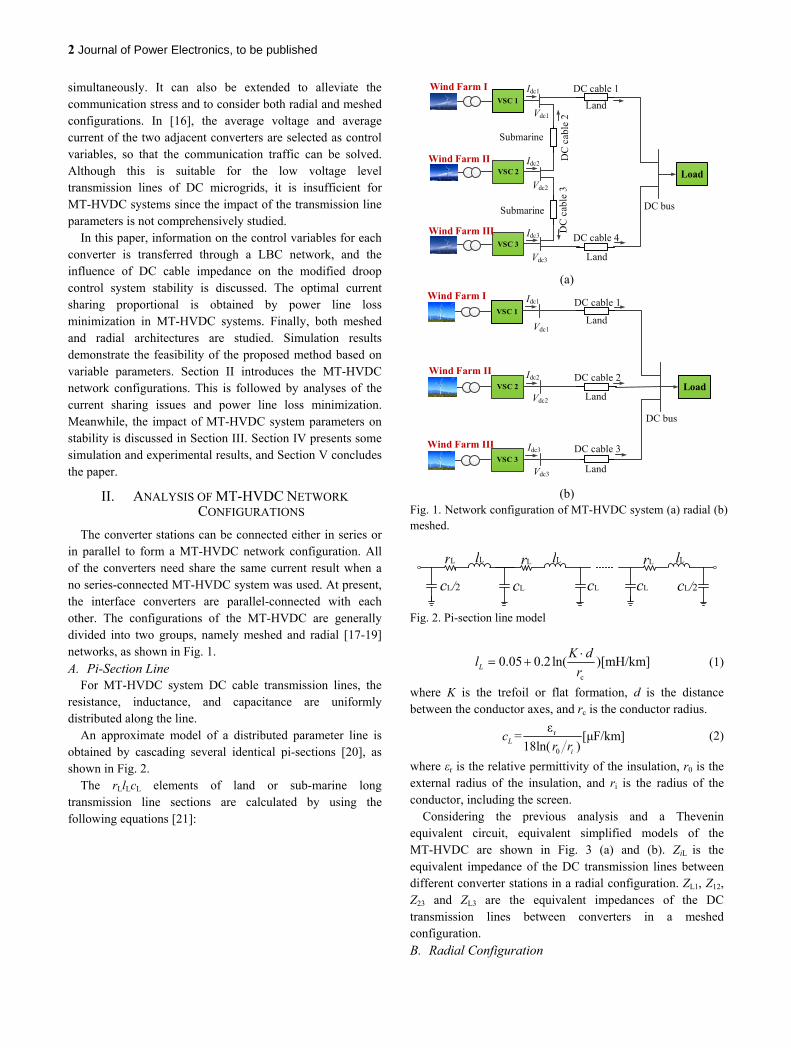
The converter stations can be connected either in series or in parallel to form a MT-HVDC network configuration. All of the converters need share the same current result when a no series-connected MT-HVDC system was used. At present, the interface converters are parallel-connected with each other. The configurations of the MT-HVDC are generally divided into two groups, namely meshed and radial [17-19] networks, as shown in Fig. 1. A. Pi-Section Line
For MT-HVDC system DC cable transmission lines, the resistance, inductance, and capacitance are uniformly distributed along the line.
An approximate model of a distributed parameter line is obtained by cascading several identical pi-sections [20], as shown in Fig. 2.
The rLlLcL elements of land or sub-marine long transmission line sections are calculated by using the following equations [21]:
Wind Farm II
VSC 1
VSC 2
Idc1
Idc2
DC cable 1
Vdc1
Vdc2
VSC 3
Wind Farm III Idc3
Vdc3
DC bus
Wind Farm I
DC
cab
le 2
DC
cab
le 3
DC cable 4
Load
Land
Submarine
Land
Submarine
(a)
VSC 1
VSC 2
Idc1
Idc2
Vdc1
Vdc2
VSC 3
Idc3
Vdc3
Wind Farm II
Wind Farm III
Wind Farm I
DC bus
Load
DC cable 1
DC cable 2
DC cable 3
Land
Land
Land
(b) Fig. 1. Network configuration of MT-HVDC system (a) radial (b) meshed.
lL
cL/2 cL
rL lLrL lLrL
cL cL cL/2
Fig. 2. Pi-section line model
c
0.05 0.2 ln( )[mH/km]L
K dl
r
(1)
where K is the trefoil or flat formation, d is the distance between the conductor axes, and rc is the conductor radius.
r
0
ε= [μF/km]
18ln( )Li
cr r
(2)
where εr is the relative permittivity of the insulation, r0 is the external radius of the insulation, and ri is the radius of the conductor, including the screen.
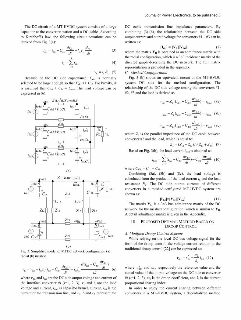
Considering the previous analysis and a Thevenin equivalent circuit, equivalent simplified models of the MT-HVDC are shown in Fig. 3 (a) and (b). ZiL is the equivalent impedance of the DC transmission lines between different converter stations in a radial configuration. ZL1, Z12, Z23 and ZL3 are the equivalent impedances of the DC transmission lines between converters in a meshed configuration. B. Radial Configuration
Journal of Power Electronics, to be published 3
The DC circuit of a MT-HVDC system consists of a large capacitor at the converter station and a DC cable. According to Kirchhoff's law, the following circuit equations can be derived from Fig. 3(a):
dc Lcc dc dc L
ii i i iL
dv dvi i C l c
dt dt (3)
3
L cci1i
i i
(4)
L L Lv i R (5)
Because of the DC side capacitance, Cdci is normally selected to be large enough so that Cdci >> CLi. For brevity, it is assumed that Cdci + CLi = Cdci. The load voltage can be expressed in (6):
vL
Z1L=l1L(rL+jωlL)
Z2L
Z3L
Cdc1+l1LcLidc1
vdc1
vdc2
vdc3
idc2
idc3
icc2
icc3
iL
l2LcL
icc1
l1LcL
RL
icL1icdc1
l3LcL
Cdc2+l2LcL
Cdc3+l3LcL
icL2icdc2
icL3icdc3
(a)
vL
ZL1=lL1(rL+jωlL)
Z23
Z12
Cdc1idc1
vdc1
idc2 idc3
iL
C13LRL
icdc1
Cdc3Cdc2
ZL3
icdc2 icdc3
Z12
Z23
ZL3
ZL1
+
_
vdc2+ vdc3+
_ _
i13Lidc1L
idc3Lidc12
idc23
(b)
Fig. 3. Simplified model of MTDC network configuration (a) radial (b) meshed.
dcdc dc
dcL dc L dc dc L
( )( )
ii i
ii iL i i iL
dvd i Cdv dtv v l r i C l l
dt dt
(6)
where vdci and idci are the DC side output voltage and current of the interface converter #i (i=1, 2, 3), vL and iL are the load voltage and current, icdci is capacitor branch current, icci is the current of the transmission line, and rL, lL and cL represent the
DC cable transmission line impedance parameters. By combining (3)-(6), the relationship between the DC side output current and output voltage for converters #1 ~ #3 can be written as:
[Idci] = [YR][Vdci] (7) where the matrix YR is obtained as an admittance matrix with the radial configuration, which is a 3×3 incidence matrix of the directed graph describing the DC network. The full matrix representation is provided in the appendix. C. Meshed Configuration
Fig. 3 (b) shows an equivalent circuit of the MT-HVDC system DC side for the meshed configuration. The relationship of the DC side voltage among the converters #1, #2, #3 and the load is derived as:
dc1dc1 L1 dc1 dc1 load( )
dvv Z i C v
dt (8a)
dc2dc2 p dc2 dc2 load( )
dvv Z i C v
dt (8b)
dc3dc3 L3 dc3 dc3 load( )
dvv Z i C v
dt (8c)
where Zp is the parallel impedance of the DC cable between converter #2 and the load, which is equal to:
L1 12 L3 23( ) / /( )pZ Z Z Z Z (9)
Based on Fig. 3(b), the load current iload is obtained as: 3
dc loadload dc dc 13L
1
( )ii i
i
dv dvi i C C
dt dt
(10)
where C13L = C1L + C3L. Combining (8a), (8b) and (8c), the load voltage is
calculated from the product of the load current iL and the load resistance RL. The DC side output currents of different converters in a meshed-configured MT-HVDC system are shown as:
[Idci]=[YM][Vdci] (11) The matrix YM is a 3×3 bus admittance matrix of the DC
network for the meshed configuration, which is similar to YR. A detail admittance matrix is given in the Appendix.
III. PROPOSED OPTIMAL METHOD BASED ON DROOP CONTROL
A. Modified Droop Control Scheme While relying on the local DC bus voltage signal for the
form of the droop control, the voltage-current relation at the traditional droop control [22] can be expressed as:
* 0dc dc dci i
i
mv v i
k (12)
where ∗ and vdci, respectively the reference value and the actual value of the output voltage on the DC side at converter #i (i=1, 2, 3), m0 is the droop coefficient, and ki is the current proportional sharing index.
In order to study the current sharing between different converters in a MT-HVDC system, a decentralized method
4 Journal of Power Electronics, to be published
based on droop control is proposed to solve this problem. According to (12), it can be seen that the given value of the DC side output voltage linearly decreases with an increase of the DC output current. Since there is no reactive power in the DC side of the MT-HVDC system, only the active current sharing accuracy should be noticed. In general, the consideration of the line impedance is inevitable due to the high DC output voltage, especially for cases with long power transmission lines.
In this paper, DC voltage deviation is eliminated and current sharing accuracy is enhanced by adding two compensation controllers to the reference value of each DC voltage. Meanwhile, the communication data of the compensation controllers are transferred from two adjacent converters through an LBC network. These controllers are achieved locally and it can achieve decentralized control. At the same time, the load current can achieve proportional sharing by compensation controller II. Then the current flow of the sharing system is modified by the outer control loop. Finally, the sharing of the DC output current is enhanced. The output voltage reference value of each converter can be obtained as:
* 0dc dc dc
dc( -1) dc( +1)*piv dc d
dc( 1) dc( +1)dcpic d
( )2
( )2
i i LPFi
i i
i ii
i
mv v i G
k
v vG v G
i iiG G
k
Compensation controller (13) where GLPF is the low pass filter, and the cutting frequency fc is set to 20 Hz. vdc(i-1), vdc(i+1), idc(i-1) and idc(i+1) are the DC side output voltage and current of the converters #(i-1) and #(i+1). Gpiv and Gpic are the transfer functions of the compensate voltage and current PI controllers, and the communication delay is shown as Gd, which can be expressed as follows:
d
1
1G
s
(14)
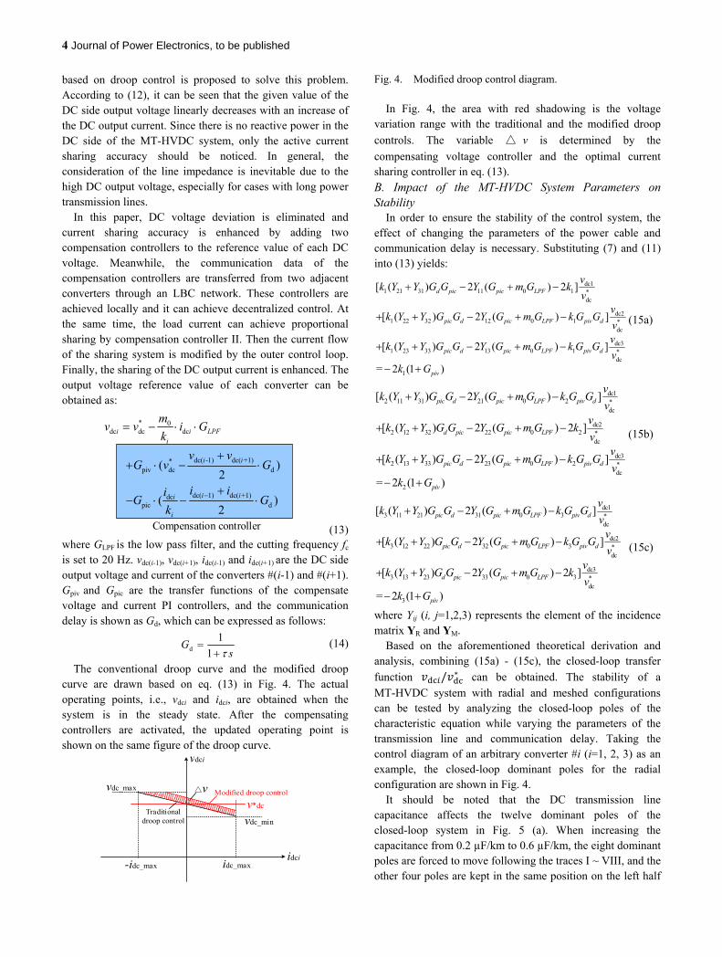
The conventional droop curve and the modified droop curve are drawn based on eq. (13) in Fig. 4. The actual operating points, i.e., vdci and idci, are obtained when the system is in the steady state. After the compensating controllers are activated, the updated operating point is shown on the same figure of the droop curve.
vdc_max
vdc_min
v*dc
idc_max
Traditional droop control
vdci
-idc_maxidci
v Modified droop control
Fig. 4. Modified droop control diagram.
In Fig. 4, the area with red shadowing is the voltage variation range with the traditional and the modified droop
controls. The variable v is determined by the
compensating voltage controller and the optimal current sharing controller in eq. (13). B. Impact of the MT-HVDC System Parameters on Stability
In order to ensure the stability of the control system, the effect of changing the parameters of the power cable and communication delay is necessary. Substituting (7) and (11) into (13) yields:
dc11 21 31 11 0 1 *
dc
dc21 22 32 12 0 1 *
dc
dc31 23 33 13 0 1 *
dc
1
[ ( ) 2 ( ) 2 ]
[ ( ) 2 ( ) ]
[ ( ) 2 ( ) ]
= 2 (1 )
d pic pic LPF
pic d pic LPF piv d
pic d pic LPF piv d
piv
vk Y Y G G Y G m G k
vv
k Y Y G G Y G m G k G Gvv
k Y Y G G Y G m G k G Gv
k G
(15a)
dc12 11 31 21 0 2 *
dc
dc22 12 32 22 0 2 *
dc
dc32 13 33 23 0 2 *
dc
2
[ ( ) 2 ( ) ]
[ ( ) 2 ( ) 2 ]
[ ( ) 2 ( ) ]
= 2 (1 )
pic d pic LPF piv d
d pic pic LPF
pic d pic LPF piv d
piv
vk Y Y G G Y G m G k G G
vv
k Y Y G G Y G m G kv
vk Y Y G G Y G m G k G G
vk G
(15b)
dc13 11 21 31 0 3 *
dc
dc23 12 22 32 0 3 *
dc
dc33 13 23 33 0 3 *
dc
3
[ ( ) 2 ( ) ]
[ ( ) 2 ( ) ]
[ ( ) 2 ( ) 2 ]
= 2 (1 )
pic d pic LPF piv d
pic d pic LPF piv d
d pic pic LPF
piv
vk Y Y G G Y G m G k G G
vv
k Y Y G G Y G m G k G Gv
vk Y Y G G Y G m G k
vk G
(15c)
where Yij (i, j=1,2,3) represents the element of the incidence matrix YR and YM.
Based on the aforementioned theoretical derivation and analysis, combining (15a) - (15c), the closed-loop transfer
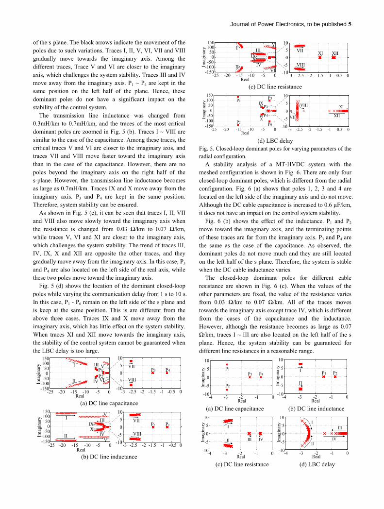
function / ∗ can be obtained. The stability of a MT-HVDC system with radial and meshed configurations can be tested by analyzing the closed-loop poles of the characteristic equation while varying the parameters of the transmission line and communication delay. Taking the control diagram of an arbitrary converter #i (i=1, 2, 3) as an example, the closed-loop dominant poles for the radial configuration are shown in Fig. 4.
It should be noted that the DC transmission line capacitance affects the twelve dominant poles of the closed-loop system in Fig. 5 (a). When increasing the capacitance from 0.2 µF/km to 0.6 µF/km, the eight dominant poles are forced to move following the traces I ~ VIII, and the other four poles are kept in the same position on the left half
Journal of Power Electronics, to be published 5
of the s-plane. The black arrows indicate the movement of the poles due to such variations. Traces I, II, V, VI, VII and VIII gradually move towards the imaginary axis. Among the different traces, Trace V and VI are closer to the imaginary axis, which challenges the system stability. Traces III and IV move away from the imaginary axis. P1 ~ P4 are kept in the same position on the left half of the plane. Hence, these dominant poles do not have a significant impact on the stability of the control system.
The transmission line inductance was changed from 0.3mH/km to 0.7mH/km, and the traces of the most critical dominant poles are zoomed in Fig. 5 (b). Traces I ~ VIII are similar to the case of the capacitance. Among these traces, the critical traces V and VI are closer to the imaginary axis, and traces VII and VIII move faster toward the imaginary axis than in the case of the capacitance. However, there are no poles beyond the imaginary axis on the right half of the s-plane. However, the transmission line inductance becomes as large as 0.7mH/km. Traces IX and X move away from the imaginary axis. P3 and P4 are kept in the same position. Therefore, system stability can be ensured.
As shown in Fig. 5 (c), it can be seen that traces I, II, VII and VIII also move slowly toward the imaginary axis when the resistance is changed from 0.03 Ω/km to 0.07 Ω/km, while traces V, VI and XI are closer to the imaginary axis, which challenges the system stability. The trend of traces III, IV, IX, X and XII are opposite the other traces, and they gradually move away from the imaginary axis. In this case, P3 and P4 are also located on the left side of the real axis, while these two poles move toward the imaginary axis.
Fig. 5 (d) shows the location of the dominant closed-loop poles while varying the communication delay from 1 s to 10 s. In this case, P1 - P6 remain on the left side of the s plane and is keep at the same position. This is are different from the above three cases. Traces IX and X move away from the imaginary axis, which has little effect on the system stability. When traces XI and XII move towards the imaginary axis, the stability of the control system cannot be guaranteed when the LBC delay is too large.
-3 -2.5 -2 -1.5 -1 -0.5 0-10
-5
0
5
10
-25 -20 -15 -10 -5 0-150-100-50
050
100150
I
II
III
IV
V
VI
VII
VIIIP2
P1 P4P3
Real
Imag
inar
y
(a) DC line capacitance
-10
-5
0
5
10
-3 -2.5 -2 -1.5 -1 -0.5 0
P4P3VII
VIII
-25 -20 -15 -10 -5 0-150-100-50
050
100150
I
II
IIIV
VIIV
IXX
Real
Imag
inar
y
(b) DC line inductance
-25 -20 -15 -10 -5 0-150-100-50
050
100150
-10
-5
0
5
10I
II
IIIV
VIIV
IXX
-3 -2.5 -2 -1.5 -1 -0.5 0
XIVII
VIII
XII
Real
Imag
inar
y
(c) DC line resistance
-25 -20 -15 -10 -5 0-150-100-50
050
100150
-3 -2.5 -2 -1.5 -1 -0.5 0-10
-5
0
5
10
VIII
X
P1
P2
P3
P4
P5
P6
IX
VII
XI
XII
Real
Imag
inar
y
(d) LBC delay
Fig. 5. Closed-loop dominant poles for varying parameters of the radial configuration.
A stability analysis of a MT-HVDC system with the meshed configuration is shown in Fig. 6. There are only four closed-loop dominant poles, which is different from the radial configuration. Fig. 6 (a) shows that poles 1, 2, 3 and 4 are located on the left side of the imaginary axis and do not move. Although the DC cable capacitance is increased to 0.6 µF/km, it does not have an impact on the control system stability.
Fig. 6 (b) shows the effect of the inductance. P1 and P2 move toward the imaginary axis, and the terminating points of these traces are far from the imaginary axis. P3 and P4 are the same as the case of the capacitance. As observed, the dominant poles do not move much and they are still located on the left half of the s plane. Therefore, the system is stable when the DC cable inductance varies.
The closed-loop dominant poles for different cable resistance are shown in Fig. 6 (c). When the values of the other parameters are fixed, the value of the resistance varies from 0.03 Ω/km to 0.07 Ω/km. All of the traces moves towards the imaginary axis except trace IV, which is different from the cases of the capacitance and the inductance. However, although the resistance becomes as large as 0.07 Ω/km, traces I ~ III are also located on the left half of the s plane. Hence, the system stability can be guaranteed for different line resistances in a reasonable range.
-4 -3 -2 -1 0-10
-5
0
5
10
P1
P2
P3 P4
Real
Imag
inar
y
-4 -3 -2 -1 0-10
-5
0
5
10
I
II
P1 P2
Real
Imag
inar
y
(a) DC line capacitance (b) DC line inductance
-4 -3 -2 -1 0-10
-5
0
5
10
I
II III IV
Real
Imag
inar
y
-4 -3 -2 -1 0-10
-5
0
5
10I
IIIV
III
Real
Imag
inar
y
(c) DC line resistance (d) LBC delay
6 Journal of Power Electronics, to be published
Fig. 6. Closed-loop dominant poles for varying parameters of the meshed configuration.
The closed-loop dominant poles of vdci/v
*dc for different
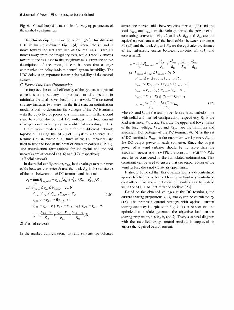
LBC delays are shown in Fig. 6 (d), where traces I and II move toward the left half side of the real axis. Trace III moves away from the imaginary axis, while Trace IV moves toward it and is closer to the imaginary axis. From the above descriptions of the traces, it can be seen that a large communication delay leads to control system instability. The LBC delay is an important factor in the stability of the control system. C. Power Line Loss Optimization
To improve the overall efficiency of the system, an optimal current sharing strategy is proposed in this section to minimize the total power loss in the network. The proposed strategy includes two steps: In the first step, an optimization model is built to determine the voltages of the DC terminals with the objective of power loss minimization; in the second step, based on the optimal DC voltages, the load current sharing accuracies k1: k2: k3 can be obtained according to (15).
Optimization models are built for the different network topologies. Taking the MT-HVDC system with three DC terminals as an example, all three of the DC terminals are used to feed the load at the point of common coupling (PCC). The optimization formulations for the radial and meshed networks are expressed as (16) and (17), respectively. 1) Radial network
In the radial configuration, vdciL is the voltage across power cable between converter #i and the load. RiL is the resistance of the line between the #i DC terminal and the load.
2 2 21 loss_radial dc1L 1 dc2L 2 dc3L 3
dcmin dc dcmax
min max dc
dc1L dc2L dc3L
dc1L dc1 L dc2L dc2 L dc3L dc3 L
dc1 L dc2 L dc3 L
1 2
min
. . ,
;
0; 0; 0
; ;
(
dciL L L
v
i
L L L MPPT i
LL L
P v R v R v R
s t V v V i
V v V P P
v v v
v v v v v v v v v
v v v v v vv
R R
L
3
)L
RR
(16)
2) Meshed network
In the meshed configuration, vdcL1 and vdcL3 are the voltages
across the power cable between converter #1 (#3) and the load, vdc12 and vdc23 are the voltage across the power cable connecting converters #1, #2 and #3. RL1 and RL3 are the equivalent resistances of the land cables between converter #1 (#3) and the load. R12 and R23 are the equivalent resistance of the submarine cables between converter #1 (#3) and converter #2.
dc
2 2 2 2dcL1 dc12 dc23 dcL3
2 loss_meshL1 12 23 L3
dcmin dc dcmax
min max dc
dcL1 dc12 dc23 dc3L
dcL1 dc1 L dc12 dc2 dc1
dc1L dc2 dc3 dcL3 dc3 L
min
. . ,
;
0; 0; 0; 0
;
;
iv
i
L L L MPPT i
v v v vP
R R R R
s t V v V i
V v V P P
v v v v
v v v v v v
v v v v v v
dc1 L dc3 LL
L1 L3
( )L
v v v vv R
R R
(17)
where λ1 and λ2 are the total power losses in transmission line with radial and meshed configuration, respectively. RL is the load resistance, VLmax and VLmin are the upper and lower limits of the load voltage, Vdcmin and Vdcmax are the minimum and maximum DC voltages of the DC terminal #i. is the set
of DC terminals. PMPPT is the maximum wind power. Pdci is the DC output power in each converter. Since the output power of a wind turbines should be no more than the maximum power point (MPP), the constraint PMPPT ≥ Pdci need to be considered in the formulated optimization. This constraint can be used to ensure that the output power of the wind turbine does not violate its upper limit.
It should be noted that this optimization is a decentralized approach which is performed locally without any centralized controllers. The above optimization models can be solved using the MATLAB optimization toolbox [23].
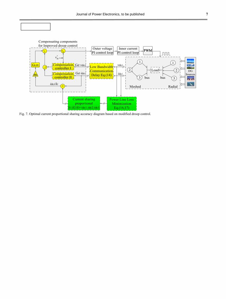
Based on the obtained voltages at the DC terminals, the current sharing proportions k1, k2 and k3 can be calculated by (15). The proposed control strategy with optimal current sharing accuracy is depicted in Fig. 7. It can be seen that the optimization module generates the objective load current sharing proportion, i.e. k1, k2 and k3. Then, a control diagram with the modified droop control method is employed to ensure the required output current.
Journal of Power Electronics, to be published 7
Local bus
3
Load
1
2
1
2
3
Meshed Radial
DG Sources
vdci
idci
bus
PWMPWM
Compensating components for Improved droop control
GLPF
m0Gd·idci
Low Bandwidth Communication Delay Eq.(14)
+ +
*dcv
idci/ki
+_
+_
÷
Gd·vdci
bus
Power Line Loss Minimization
Eq.(16,17)
Current sharing proportional
k1:k2:k3=idc1:idc2:idc3
Compensation controller I
Compensation controller II
Outer voltagePI control loop
Inner currentPI control loop
Fig. 7. Optimal current proportional sharing accuracy diagram based on modified droop control.

Journal of Power Electronics, to be published 1
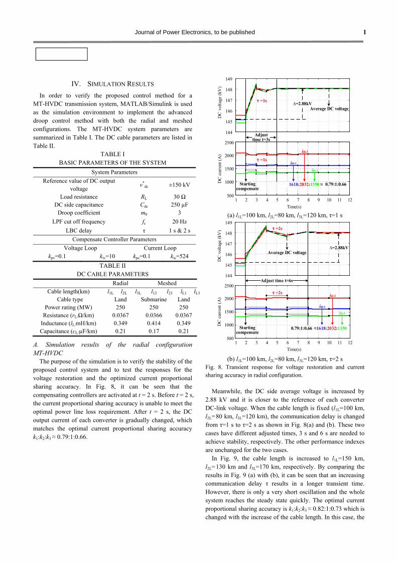
IV. SIMULATION RESULTS
In order to verify the proposed control method for a MT-HVDC transmission system, MATLAB/Simulink is used as the simulation environment to implement the advanced droop control method with both the radial and meshed configurations. The MT-HVDC system parameters are summarized in Table I. The DC cable parameters are listed in Table II.
TABLE I BASIC PARAMETERS OF THE SYSTEM
System Parameters
Reference value of DC output voltage
v*dc ±150 kV
Load resistance RL 30 Ω DC side capacitance Cdc 250 µF
Droop coefficient m0 3
LPF cut off frequency fc 20 Hz
LBC delay τ 1 s & 2 s
Compensate Controller Parameters
Voltage Loop Current Loop kpv=0.1 kiv=10 kpc=0.1 kic=524
TABLE II DC CABLE PARAMETERS
Radial Meshed Cable length(km) l1L l2L l3L l12 l23 lL1 lL3
Cable type Land Submarine Land Power rating (MW) 250 250 250
Resistance (rL/Ω/km) 0.0367 0.0366 0.0367Inductance (lL/mH/km) 0.349 0.414 0.349 Capacitance (cL/µF/km) 0.21 0.17 0.21
A. Simulation results of the radial configuration MT-HVDC
The purpose of the simulation is to verify the stability of the proposed control system and to test the responses for the voltage restoration and the optimized current proportional sharing accuracy. In Fig. 8, it can be seen that the compensating controllers are activated at t = 2 s. Before t = 2 s, the current proportional sharing accuracy is unable to meet the optimal power line loss requirement. After t = 2 s, the DC output current of each converter is gradually changed, which matches the optimal current proportional sharing accuracy k1:k2:k3 ≈ 0.79:1:0.66.
Adjust time t=3s
1 2 3 4 5 6 7 8 9 10 11 12500
1000
1500
2000
2500
Time(s)
DC
cur
rent
(A
)
144
145
146
147
148
149
DC
vol
tage
(kV
)
Average DC voltage
τ =1s
1618:2032:1350 ≈ 0.79:1:0.66
τ =1s
Starting compensate
idc1
idc2
idc3
(a) l1L=100 km, l2L=80 km, l3L=120 km, τ=1 s
1 2 3 4 5 6 7 8 9 10 11 12500
1000
1500
2000
2500
Time(s)
DC
cur
rent
(A
)
144
145
146
147
148
149 D
C v
olta
ge (
kV)
τ =2s
≈1618:2032:1350 0.79:1:0.66
τ =2s
Starting compensate
Average DC voltage
idc1
idc2
idc3
(b) l1L=100 km, l2L=80 km, l3L=120 km, τ=2 s
Fig. 8. Transient response for voltage restoration and current sharing accuracy in radial configuration.
Meanwhile, the DC side average voltage is increased by 2.88 kV and it is closer to the reference of each converter DC-link voltage. When the cable length is fixed (l1L=100 km, l2L=80 km, l3L=120 km), the communication delay is changed from τ=1 s to τ=2 s as shown in Fig. 8(a) and (b). These two cases have different adjusted times, 3 s and 6 s are needed to achieve stability, respectively. The other performance indexes are unchanged for the two cases.
In Fig. 9, the cable length is increased to l1L=150 km, l2L=130 km and l3L=170 km, respectively. By comparing the results in Fig. 9 (a) with (b), it can be seen that an increasing communication delay τ results in a longer transient time. However, there is only a very short oscillation and the whole system reaches the steady state quickly. The optimal current proportional sharing accuracy is k1:k2:k3 ≈ 0.82:1:0.73 which is changed with the increase of the cable length. In this case, the
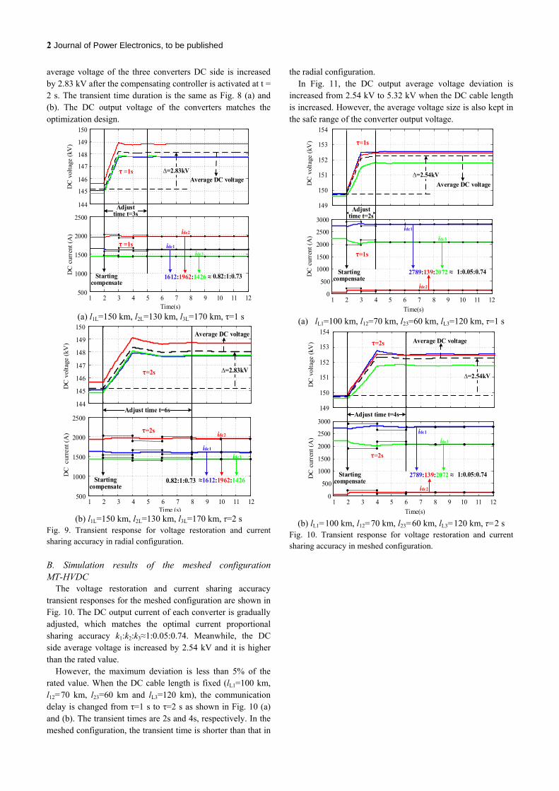
2 Journal of Power Electronics, to be published
average voltage of the three converters DC side is increased by 2.83 kV after the compensating controller is activated at t = 2 s. The transient time duration is the same as Fig. 8 (a) and (b). The DC output voltage of the converters matches the optimization design.
144
146
148
150
Time(s)
DC
cur
rent
(A
) D
C v
olta
ge (
kV)
1 2 3 4 5 6 7 8 9 10 11 12500
1000
1500
2000
2500
Adjust time t=3s
Average DC voltage
1612:1962:1426 ≈ 0.82:1:0.73
τ =1s
Starting compensate
τ =1s
145
147
149
idc1
idc2
idc3
(a) l1L=150 km, l2L=130 km, l3L=170 km, τ=1 s
144
145
146
147
148
149
150
DC
vol
tage
(kV
)
1 2 3 4 5 6 7 8 9 10 11 12500
1000
1500
2000
2500
Time (s)
DC
cur
rent
(A
)
∆=2.83kV
Average DC voltage
τ=2s
≈1612:1962:1426 0.82:1:0.73
Adjust time t=6s
Starting compensate
τ=2s
idc1
idc2
idc3
(b) l1L=150 km, l2L=130 km, l3L=170 km, τ=2 s
Fig. 9. Transient response for voltage restoration and current sharing accuracy in radial configuration.
B. Simulation results of the meshed configuration MT-HVDC
The voltage restoration and current sharing accuracy transient responses for the meshed configuration are shown in Fig. 10. The DC output current of each converter is gradually adjusted, which matches the optimal current proportional sharing accuracy k1:k2:k3≈1:0.05:0.74. Meanwhile, the DC side average voltage is increased by 2.54 kV and it is higher than the rated value.
However, the maximum deviation is less than 5% of the rated value. When the DC cable length is fixed (lL1=100 km, l12=70 km, l23=60 km and lL3=120 km), the communication delay is changed from τ=1 s to τ=2 s as shown in Fig. 10 (a) and (b). The transient times are 2s and 4s, respectively. In the meshed configuration, the transient time is shorter than that in
the radial configuration. In Fig. 11, the DC output average voltage deviation is
increased from 2.54 kV to 5.32 kV when the DC cable length is increased. However, the average voltage size is also kept in the safe range of the converter output voltage.
Adjust time t=2s
1 2 3 4 5 6 7 8 9 10 11 12
Time(s) D
C c
urre
nt (
A)
DC
vol
tage
(kV
)
0
500
1000
1500
2000
2500
3000
149
150
151
152
153
154
Average DC voltage
τ=1s
2789:139:2072 ≈ 1:0.05:0.74
τ=1s
Starting compensate
idc1
idc2
idc3
(a) lL1=100 km, l12=70 km, l23=60 km, lL3=120 km, τ=1 s
1 2 3 4 5 6 7 8 9 10 11 12
Time(s)
DC
cur
rent
(A
) D
C v
olta
ge (
kV)
0
500
1000
1500
2000
2500
3000
149
150
151
152
153
154Average DC voltage τ=2s
2789:139:2072 ≈ 1:0.05:0.74
τ=2s
Adjust time t=4s
Starting compensate
idc1
idc2
idc3
(b) lL1=100 km, l12=70 km, l23=60 km, lL3=120 km, τ=2 s
Fig. 10. Transient response for voltage restoration and current sharing accuracy in meshed configuration.
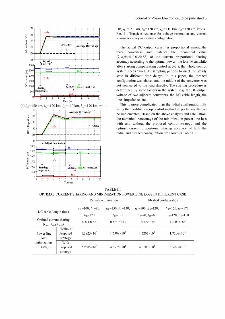
Journal of Power Electronics, to be published 3
Adjust time t=2s
148
150
152
154
156
158D
C v
olta
ge (
kV)
1 2 3 4 5 6 7 8 9 10 11 120
500
1000
1500
2000
2500
3000
Time (s)
DC
cur
rent
(A
)
Average DC voltage
τ =1s
2622:72:2306 ≈ 1:0.03:0.88
τ =1s
Starting compensate
idc1
idc2
idc3
(a) lL1=150 km, l12=120 km, l23=110 km, lL3=170 km, τ=1 s
0
500
1000
1500
2000
2500
3000
DC
cur
rent
(A
)
1 2 3 4 5 6 7 8 9 10 11 12
148
150
152
154
156
158
DC
vol
tage
(kV
)
Time (s)
Average DC voltage
τ=2s
2622:72:2306 ≈ 1:0.03:0.88
τ=2s
Adjust time t=4s
Starting compensate
idc1
idc2
idc3
(b) lL1=150 km, l12=120 km, l23=110 km, lL3=170 km, τ=2 s Fig. 11. Transient response for voltage restoration and current sharing accuracy in meshed configuration.
The actual DC output current is proportional among the three converters and matches the theoretical value (k1:k2:k3≈1:0.03:0.88) of the current proportional sharing accuracy according to the optimal power line loss. Meanwhile, after starting compensating control at t=2 s, the whole control system needs two LBC sampling periods to meet the steady state in different time delays. In this paper, the meshed configuration was chosen and the middle of the converter was not connected to the load directly. The starting procedure is determined by some factors in the system, e.g. the DC output voltage of two adjacent converters, the DC cable length, the lines impedance, etc.
This is more complicated than the radial configuration. By using the modified droop control method, expected results can be implemented. Based on the above analysis and calculation, the numerical percentage of the minimization power line loss with and without the proposed control strategy and the optimal current proportional sharing accuracy of both the radial and meshed configuration are shown in Table III.
TABLE III OPTIMAL CURRENT SHARING AND MINIMIZATION POWER LINE LOSS IN DIFFERENT CASE
Radial configuration Meshed configuration
DC cable Length (km) l1L=100; l2L=80;
l3L=120
l1L=150; l2L=130;
l3L=170
lL1=100; lL3=120;
l12=70; l12=60
lL1=150; lL3=170;
l12=120; l12=110 Optimal current sharing
(kopt1:kopt2:kopt3) 0.8:1:0.68 0.82:1:0.73 1:0.05:0.74 1:0.03:0.88
Power line loss
minimization (kW)
Without Proposed strategy
1.3825×10⁵ 1.5509×10⁵ 1.5202×10⁵ 1.7206×10⁵
With Proposed strategy
2.9505×10⁴ 4.3576×10⁴ 4.5185×10⁴ 6.5995×10⁴
Journal of Power Electronics, to be published 2
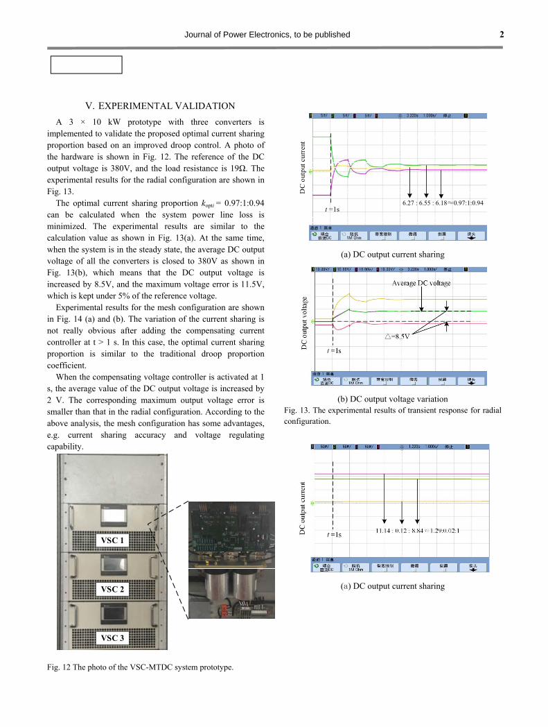
V. EXPERIMENTAL VALIDATION
A 3 × 10 kW prototype with three converters is implemented to validate the proposed optimal current sharing proportion based on an improved droop control. A photo of the hardware is shown in Fig. 12. The reference of the DC output voltage is 380V, and the load resistance is 19Ω. The experimental results for the radial configuration are shown in Fig. 13.
The optimal current sharing proportion kopti = 0.97:1:0.94 can be calculated when the system power line loss is minimized. The experimental results are similar to the calculation value as shown in Fig. 13(a). At the same time, when the system is in the steady state, the average DC output voltage of all the converters is closed to 380V as shown in Fig. 13(b), which means that the DC output voltage is increased by 8.5V, and the maximum voltage error is 11.5V, which is kept under 5% of the reference voltage.
Experimental results for the mesh configuration are shown in Fig. 14 (a) and (b). The variation of the current sharing is not really obvious after adding the compensating current controller at t > 1 s. In this case, the optimal current sharing proportion is similar to the traditional droop proportion coefficient.
When the compensating voltage controller is activated at 1 s, the average value of the DC output voltage is increased by 2 V. The corresponding maximum output voltage error is smaller than that in the radial configuration. According to the above analysis, the mesh configuration has some advantages, e.g. current sharing accuracy and voltage regulating capability.
VSC 1
VSC 2
VSC 3
Fig. 12 The photo of the VSC-MTDC system prototype.
t =1s
DC
out
put c
urre
nt
6.27 : 6.55 : 6.18≈0.97:1:0.94
(a) DC output current sharing
(b) DC output voltage variation Fig. 13. The experimental results of transient response for radial configuration.
(a) DC output current sharing
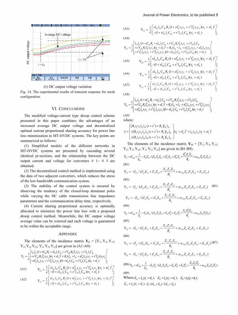
Journal of Power Electronics, to be published 3
(b) DC output voltage variation Fig. 14. The experimental results of transient response for mesh configuration.
VI. CONCLUSIONS
The modified voltage-current type droop control scheme presented in this paper combines the advantages of an increased average DC output voltage and decentralized optimal current proportional sharing accuracy for power line loss minimization in MT-HVDC systems. The key points are summarized as follows:
(1) Simplified models of the different networks in MT-HVDC systems are presented by cascading several identical pi-sections, and the relationship between the DC output current and voltage for converters # 1~ # 3 are obtained.
(2) The decentralized control method is implemented using the data of two adjacent converters, which reduces the stress of the low bandwidth communication system.
(3) The stability of the control system is ensured by observing the tendency of the closed-loop dominant poles while varying the DC cable transmission line impedance parameters and the communication delay time, respectively.
(4) Current sharing proportional accuracy is optimally allocated to minimize the power line loss with a proposed droop control method. Meanwhile, the DC output voltage average value can be restored and each voltage is guaranteed to be within the acceptable range.
APPENDIX
The elements of the incidence matrix YR = [Y11 Y12 Y13; Y21 Y22 Y23; Y31 Y32 Y33] are given in (A1-A9).
2 2 22L 3L dc L 1L L dc dc L 1L L L 1L L dc
3 2 2 2 2 211 dc L 1L L L L L L 3L 2L 2L 3L L L 2L 3 L L
2 2 2 23L 2L L L 3L 2L L L 1L L dc 1L L dc L L
(11
Y )( ) ()(1 )( )
l l sC R sl l C s C R l r c s l l Cs C R l r c r sl R l l sl l r c s l r csl l r c s l l r c sl l C s l l C r sl
(A1)2 2 2 2
2L 3L dc L 2L L L 2L L L L L212
2L L dc 2L L dc L L
1 (1 )( )Y(1 )( )
sl l C R sl r c s l r c r slsl l C s l l C r sl
(A2)2 2 2 2
2 L 3L dc L 2L L L 2L L L L L13 2
2L L dc 2L L dc L L
(1 )( )1Y
(1 )( )
sl l C R sl r c s l r c r sl
sl l C s l l C r sl
(A3)2 2 2 2
1L 3L dc L 1L L L 1L L L L L21 2
1L L dc 1L L dc L L
(1 )( )1Y
(1 )( )
sl l C R sl r c s l r c r sl
sl l C s l l C r sl
(A4)2 2 2
1L 3L dc L 2L L dc dc L 2L L L 2L L dc3 2 2 2 2
22 dc L 2L L L L L L 3L 1L 1L 3L L L 3L 1L L L2 2 2 2 2
1L 3L L L 3L 1L L L 2L L dc 2L L dc L L
(11
Y )( ) ()(1 )( )
l l sC R sl l C s C R l r c s l l Cs C R l r c r sl R l l sl l r c sl l r cs l l r c s l l r c sl l C s l l C r sl
(A5)2 2 2 2
1L 3L dc L 3L L L 3L L L L L23 2
3L L dc 3L L dc L L
(1 )( )1Y
(1 )( )
sl l C R sl r c s l r c r sl
sl l C s l l C r sl
(A6)2 2 2 2
1L 2L dc L 1L L L 1L L L L L31 2
1L L dc 1L L dc L L
(1 )( )1Y
(1 )( )
sl l C R sl r c s l r c r sl
sl l C s l l C r sl
(A7)2 2 2 2
1L 2L dc L 2L L L 2L L L L L32 2
2L L dc 2L L dc L L
(1 )( )1Y
(1 )( )
sl l C R sl r c s l r c r sl
sl l C s l l C r sl
(A8) 2 2 2
1L 2L dc L 3L L dc dc L 3L L L 3L L dc3 2 2 2 2 2
33 dc L 3L L L L L L 2L 1L 1L 2L L L 1L 2L L L2 2 2 22L 1L L L 2L 1L L L 3L L dc 3L L dc L L
(11
Y )( ) ()(1 )( )
l l sC R sl l C s C R l r c s l l Cs C R l r c r sl R l l sl l r c s l l r csl l r c s l l r c sl l C s l l C r sl
(A9)
where: 2
L L L 1L 3L L 1L 2L
2 2 3L L L 1L 2L L 2L 3L L L 1L 2L 3L L L
2L L L 2L 3L L 1L 3L
[ ( ) ]
[ ( ) ] ( ) ( )
[ ( ) ]
R r c l l s s R l l
R r c l l s s R l l r sl l l l r sl
R r c l l s s R l l
The elements of the incidence matrix YM = [Y11 Y12 Y13; Y21 Y22 Y23; Y31 Y32 Y33] are given in (B1-B9).
2L1 L32 2 2
11 dc1 L3 L1 L3 L1 L3 L1 13L L1 L3L1 L
1Y /( )p
p p p p
Z Z ZsC Z Z Z Z Z Z Z Z Z sc Z Z Z
Z R
(B1)
L1 L312 L3 L1 L3 13L L1 L3 L1 L3
L
Y / ( )pp p p
Z Z ZZ Z Z Z Z sc Z Z Z Z Z
R
(B2)
L1 L313 L1 L3 L3 13L L1 L3 L1
L
Y / ( )pp p p p
Z Z ZZ Z Z Z Z sc Z Z Z Z Z
R (B3)
L1 L321 L3 L1 L3 13L L1 L3 L1 L3
L
Y / ( )pp p p
Z Z ZZ Z Z Z Z sc Z Z Z Z Z
R
(B4) 2
L1 L32 2 222 dc2 L1 L3 L1 L3 L1 L3 13L L1 L3
L
1Y /( )p
p p p pp
Z Z ZsC Z Z Z Z Z Z Z Z Z sc Z Z Z
Z R
(B5)
L1 L323 L1 L1 L3 13L L1 L3 L1 L3
L
Y / ( )pp p p
Z Z ZZ Z Z Z Z sc Z Z Z Z Z
R
(B6)
L1 L331 L1 L3 L3 13L L1 L3 L1
L
Y / ( )pp p p p
Z Z ZZ Z Z Z Z sc Z Z Z Z Z
R (B7)
L1 L332 L1 L1 L3 13L L1 L3 L1 L3
L
Y / ( )pp p p
Z Z ZZ Z Z Z Z sc Z Z Z Z Z
R
(B8)2
L1 L32 2 233 dc3 L1 L1 L3 L1 L3 L3 13L L1 L3
L3 L
1Y /( )p
p p p p
Z Z ZsC Z Z Z Z Z Z Z Z Z sc Z Z Z
Z R
(B9)
Where L1 L1 L L( )Z l r sl , 12 12 L L( )Z l r sl , 23 23 L L( )Z l r sl ,
L3 L3 L L( )Z l r sl ,L1 12 L3 23=( ) / /( )pZ Z Z Z Z
4 Journal of Power Electronics, to be published
REFERENCES
[1]. K. Rouzbehi, A. Miranian, A. Luna, P. Rodriguez, “DC Voltage Control and Power Sharing in Multiterminal DC Grids Based on Optimal DC Power Flow and Voltage-Droop Strategy”, IEEE Journal of Emerging and Selected Topics in Power Electronics, Vol. 2, No. 4, pp.1171-1180,Dec.2014.
[2]. Z. Wei, Y. Yuan, X. Lei, H. Wang, G. Sun and Y. Sun, "Direct-Current Predictive Control Strategy for Inhibiting Commutation Failure in HVDC Converter," in IEEE Transactions on Power Systems, vol. 29, no. 5, pp. 2409-2417, Sept. 2014.
[3]. X. Shi, Z. Wang, B. Liu, Y. Liu, L. M. Tolbert and F. Wang, "Characteristic Investigation and Control of a Modular Multilevel Converter-Based HVDC System Under Single-Line-to-Ground Fault Conditions," in IEEE Transactions on Power Electronics, vol. 30, no. 1, pp. 408-421, Jan. 2015.
[4]. T. M. Haileselassie and K. Uhlen, "Impact of DC Line Voltage Drops on Power Flow of MTDC Using Droop Control," in IEEE Transactions on Power Systems, vol. 27, no. 3, pp. 1441-1449, Aug. 2012.
[5]. B. Sfurtoc, R. da Silva and S. Chaudhary, "A MTDC system layout review based on system revenue a Kriegers Flak case study," Power Engineering, Energy and Electrical Drives (POWERENG), 2013 Fourth International Conference on, Istanbul, 2013, pp. 793-800.
[6]. F. Deng, C.Z. Zhe, “An off-shore wind farm with DC grid connection and its performance under power system transients”, 2011 IEEE Power and Energy Society General Meeting, pp.24-29, Jul. 2011.
[7]. C. Li, P. Zhan, J. Wen, M. Yao, N. Li and W. J. Lee, "Offshore Wind Farm Integration and Frequency Support Control Utilizing Hybrid Multiterminal HVDC Transmission," in IEEE Transactions on Industry Applications, vol. 50, no. 4, pp. 2788-2797, July-Aug. 2014.
[8]. J. Ren, K. Li, L. Sun, J. Zhao, Y. Liang, W. Lee, Z. Ding, Y. Sun, “A coordination control strategy of voltage source converter based MTDC for off-shore wind farms”, IEEE Industry Applications Society Annual Meeting, pp.5-9, Oct. 2014.
[9]. S.J. Shao, V.G. Agelidis, “Review of DC System Technologies for Large Scale Integration of Wind Energy Systems with Electricity Grids”, Energies, Vol. 3, pp. 1303-1319, 2010.
[10]. S. Rodrigues, R.T. Pinto, P. Bauer, J. Pierik, “Optimal Power Flow Control of VSC-Based Multiterminal DC Network for off-shore Wind Integration in the North Sea”, IEEE Journal of Emerging and Selected Topics in Power Electronics, Vol. 1, No. 4, pp.260-268, Dec. 2013.
[11]. W. Li, Mi Sa-Nguyen Thi., “Power flow control of off-shore wind farms fed to power grids using an HVDC system”, 2012 IEEE Industry Applications Society Annual Meeting (IAS), pp.7-11, Oct. 2012.
[12]. X. Sun, Y.S. Lee, D.H. Xu, “Modeling, analysis, and implementation of parallel multi-inverter systems with instantaneous average-current-sharing scheme”, IEEE Trans. Power Electron., Vol. 18, No. 3, pp. 844–856, May. 2003.
[13]. X.N. Lu, J.M. Guerrero, K. Sun, J.C. Vasquez, R. Teodorescu, L.P. Huang. “Hierarchical Control of Parallel
AC-DC Converter Interfaces for Hybrid Microgrids”, IEEE Transactions on Smart Grid, Vol.5, No.2, pp.683-692, Mar. 2014.
[14]. W. Wang, M. Barnes, “Power Flow Algorithms for Multi-Terminal VSC-HVDC With Droop Control”, IEEE Transactions on Power Systems, Vol. 29, No. 4, pp.1721-1730, Jul. 2014.
[15]. X.N. Lu, J.M. Guerrero, K. Sun, J.C. Vasquez, “An Improved Droop Control Method for DC Microgrids Based on Low Bandwidth Communication With DC Bus Voltage Restoration and Enhanced Current Sharing Accuracy”, IEEE Transactions on Power Electronics, Vol. 29, No. 4, pp.1800-1812, Apr. 2014.
[16]. Y.Q. Liu, J.Z. Wang, N.N. Li, Y. Fu, Y.C. Ji, “Enhanced Load Power Sharing Accuracy in Droop-Controlled DC Microgrids with Both Mesh and Radial Configurations”. Energies, Vol.8, pp. 3591-3605, Apr. 2015.
[17]. J. Beerten, S. Cole, R. Belmans, “Modeling of Multi-Terminal VSC HVDC Systems With Distributed DC Voltage Control”, IEEE Transactions on Power Systems, Vol. 29, No.1, pp.34-42, Jan. 2014.
[18]. G.O. Kalcon, G.P. Adam, Anaya-Lara, O. Lo, S. K. Uhlen, “Small-Signal Stability Analysis of Multi-Terminal VSC-Based DC Transmission Systems”, IEEE Transactions on Power Systems, Vol. 27, No. 4, pp. 1818-1830, Nov. 2012.
[19]. R.T. Pinto, P. Bauer, S.F. Rodrigues, etc., “A Novel Distributed Direct-Voltage Control Strategy for Grid Integration of off-shore Wind Energy Systems Through MTDC Network”, IEEE Transactions on Industrial Electronics, Vol. 60, No. 6, pp.2429-2441, Jun. 2013.
[20]. S. Lin, C. Yeh, “Microstrip branch-line coupler with optimized spurious suppression based on cascaded PI-type equivalent transmission lines”, 2014 IEEE International Workshop on Electromagnetics, pp. 4-6, Aug. 2014.
[21]. An introduction to high voltage direct current (HVDC) underground cable,” Europacable, Brussels, 2011
[22]. K. Rouzbehi, A. Miranian, J.I. Candela, A. Luna, P. Rodriguez, “A Generalized Voltage Droop Strategy for Control of Multiterminal DC Grids”, IEEE Transactions on Industry Applications, Vol. 51, No. 1, pp. 607-618, Jan. 2015.
[23]. A-P. Mònica, E-À. Agustí, G-A. Samuel, G-B. Oriol: “Droop control for loss minimization in HVDC multi-terminal transmission systems for large off-shore wind farms”, Electric Power Systems Research, Vol. 112, No.1, pp.48-55, Apr. 2014.
Yiqi Liu received his B.S. degree in Electrical Engineering from the Northeast Agriculture University, Harbin, China, in 2009; and his M.S. degree in Electrical Engineering from the Tianjin University of Technology, Tianjin, China, in 2012. He is presently working towards his Ph.D. degree in the School of Electrical Engineering and Automation, Harbin
Institute of Technology, Harbin, China. From 2013 to 2015, he was a Visiting Ph.D. student with the Center for Ultra-Wide-Area Resilient Electric Energy Transmission Networks (CURENT), University of Tennessee, Knoxville, TN, USA, with support from China Scholarship Council. He joined the Northeast Forestry University, Harbin, China, in 2016, and is

Journal of Power Electronics, to be published 5
presently working as an Associate Professor. His current research interests include power electronics for renewable energy sources, multilevel converters, high-voltage direct-current (HVDC) technology, DC micro-grids and energy conversion.
Wenlong Song received his B.S., M.S., and Ph.D. degrees in Electrical Engineering from the Northeast Forestry University, Harbin, China, in 1995, 2004, and 2008, respectively. He joined the Northeast Forestry University, in 1995, and is presently working as a full Professor. His current research interests include forestry engineering automation, plant
life information detection, automation control technology, etc.
Ningning Li received his B.S. and M.S. degrees in Electronics Engineering from the Northeast Agriculture University, Harbin, China, in 2005 and 2010, respectively; and his Ph.D. degree in Electrical Engineering from the Harbin Institute of Technology, Harbin, China, in 2016. He joined the Northeast Agricultural University, in 2016, and is
presently working as a Lecturer. His current research interests include power electronics and drives, renewable energy generation and applications, FACTS, and power quality.
Linquan Bai received his B.S. and M.S. degrees in Electrical Engineering both from Tianjin University, China in 2010 and 2013 respectively. He is working towards his Ph.D. degree at the University of Tennessee, Knoxville, USA. His research interests include electricity markets, microgrid optimal
operation and planning, and integrated energy systems.
Yanchao Ji received the B.S. and M.S. degrees in electrical engineering from Northeast Dianli University, Jilin, China, in 1983 and 1989, respectively, and the Ph.D. degree in electrical engineering from the North China Electric Power University, Beijing, China, in 1993. He joined the Department of Electrical Engineering, Harbin
Institute of Technology, Harbin, China, in 1993. From 1995 to 1996, he was an Associate Professor with the Department of Electrical Engineering, Harbin Institute of Technology, where he is currently a Professor. His current research interests include pulse width modulation technique, power converter, and flexible ac transmission systems device