Review Article 1

A critical synthesis of remotely sensed optical image change detection techniques 2

Andrew P. Tewkesbury (andrew.tewkesbury@astrium.eads.net) a,b,*, Alexis J. Comber (ajc36@leicester.ac.uk) 3

b, Nicholas J. Tate (njt9@leicester.ac.uk) b, Alistair Lamb (alistair.Lamb@astrium.eads.net) a, Peter F. Fisher b 4

a Airbus Defence and Space, 6 Dominus Way, Meridian Business Park, Leicester, LE19 1RP, UK 5

b Department of Geography, University of Leicester, Leicester, LE1 7RH, UK 6

*Corresponding author: Andrew Tewkesbury, +44 (0)116 240 7200 7

Abstract 8

State of the art reviews of remote sensing change detection are becoming increasingly complicated and 9

disparate due to an ever growing list of techniques, algorithms and methods. To provide a clearer, synoptic 10

view of the field this review has organised the literature by the unit of analysis and the comparison method 11

used to identify change. This significantly reduces the conceptual overlap present in previous reviews giving a 12

succinct nomenclature with which to understand and apply change detection workflows. Under this 13

framework, several decades of research has been summarised to provide an overview of current change 14

detection approaches. Seven units of analysis and six comparison methods were identified and described 15

highlighting the advantages and limitations of each within a change detection workflow. Of these, the pixel 16

and post-classification change methods remain the most popular choices. In this review we extend previous 17

summaries and provide an accessible description of the field. This supports future research by placing a clear 18

separation between the analysis unit and the change classification method. This separation is then discussed, 19

providing guidance for applied change detection research and future benchmarking experiments. 20

Keywords 21

Remote sensing, change detection, pixel-based, object-based, land use land cover change (LULCC) 22

1. Introduction 23

Remote sensing change detection is a disparate, highly variable and ever-expanding area of research. There 24

are many different methods in use, developed over several decades of satellite remote sensing. These 25

approaches have been consolidated in several reviews (Coppin et al., 2004; Hussain et al., 2013; Lu et al., 2004; 26

Radke et al., 2005; Warner et al., 2009) and even reviews of reviews (İlsever & Ünsalan, 2012), each aiming to 27

better inform applied research and steer future developments. However, most authors agree that a universal 28

change detection technique does not yet exist (Ehlers et al., 2014) leaving end-users of the technology with an 29

increasingly difficult task selecting a suitable approach. For instance Lu et al. (2004) present seven categories 30

divided into 31 techniques, making an overall assessment very difficult. Recent advances in Object Based 31

Image Analysis (OBIA) have also further complicated this picture by presenting two parallel streams of 32

techniques (G. Chen et al., 2012; Hussain et al., 2013) with significant conceptual overlaps. For instance, direct 33

image comparison and direct object comparison (Hussain et al., 2013) could relate to identical operations 34

applied to different analysis units. This review provides a clearer nomenclature with less conceptual overlap by 35

providing a clear separation between the unit of analysis, be it the pixel or image-object, and the comparison 36

method used to highlight change. 37

Previous reviews (Hussain et al., 2013; Lu et al., 2004) have identified three broad stages in a remote sensing 38

change detection project, namely pre-processing, change detection technique selection and accuracy 39

assessment. This review focuses on the second stage, aiming to bring an improved clarity to a change 40

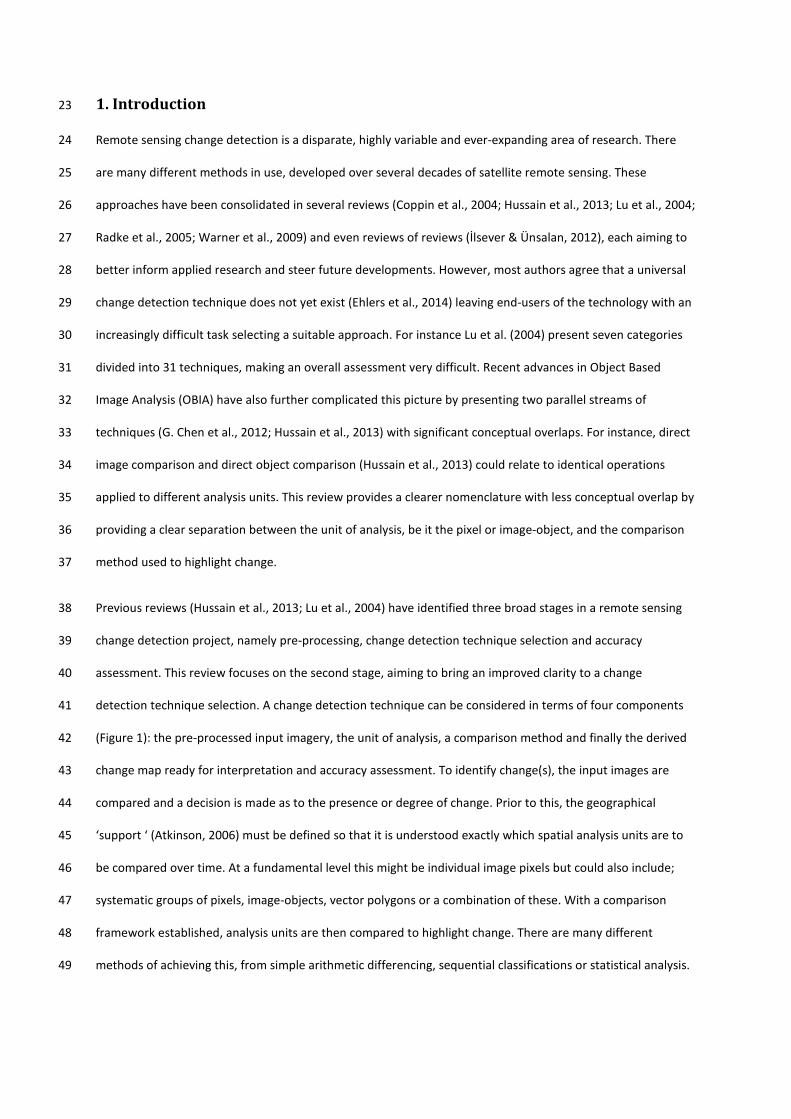
detection technique selection. A change detection technique can be considered in terms of four components 41

(Figure 1): the pre-processed input imagery, the unit of analysis, a comparison method and finally the derived 42

change map ready for interpretation and accuracy assessment. To identify change(s), the input images are 43

compared and a decision is made as to the presence or degree of change. Prior to this, the geographical 44

‘support ‘ (Atkinson, 2006) must be defined so that it is understood exactly which spatial analysis units are to 45

be compared over time. At a fundamental level this might be individual image pixels but could also include; 46

systematic groups of pixels, image-objects, vector polygons or a combination of these. With a comparison 47

framework established, analysis units are then compared to highlight change. There are many different 48

methods of achieving this, from simple arithmetic differencing, sequential classifications or statistical analysis. 49

This comparison results in a ‘change’ map which may depict the apparent magnitude of change, the type of 50

change or a combination of both. 51

52

Figure 1. A schematic showing the four components of a change detection technique. 53

2. Unit of Analysis 54

Modern remote sensing and image processing facilitate the comparison of images under several different 55

frameworks. In the broadest sense image pixels and image-objects are the two main categories of analysis 56

unit presented in the change detection literature (G. Chen et al., 2012; Hussain et al., 2013). When further 57

exploring the possible interactions, there are in fact many more permutations by which a change comparison 58

can be made. For instance, image pixels may be considered individual autonomous units or part of a 59

systematic group such as a kernel filter or moving window. Listner and Niemeyer (2011a) outlined three 60

different scenarios of image-object comparison; those generated independently, those generated from a 61

multi-temporal data stack, and lastly a simple overlay operation. In addition to these one could also consider 62

mapping objects, typically vector polygons derived from field survey, or stereo or mono photogrammetry 63

(Comber et al., 2004b; Sofina et al., 2012; Walter, 2004). Furthermore, a mixture of analysis units may be 64

utilised, with this strategy sometimes referred to as a hybrid approach (G. Chen et al., 2012; Hussain et al., 65

Image T0

Image T1

Image Tn

Unit of Analysis

Comparison method

Change map

Pixel Kernel

Image-object overlay Image-object comparison

Multi-temporal image-object Vector polygon

Hybrid

Layer arithmetic Post-classification Direct classification

Transformation Change vector analysis

Hybrid

1 2 3 4

Pre-processed imagery

Magnitude Type

2013). We discuss these elements in seven categories, namely pixel, kernel, image-object overlay, image-66

object comparison, multi-temporal image-object, vector polygon and hybrid. These categories are summarised 67

in Table 1 to include a brief description of each, advantages and disadvantages and some examples from the 68

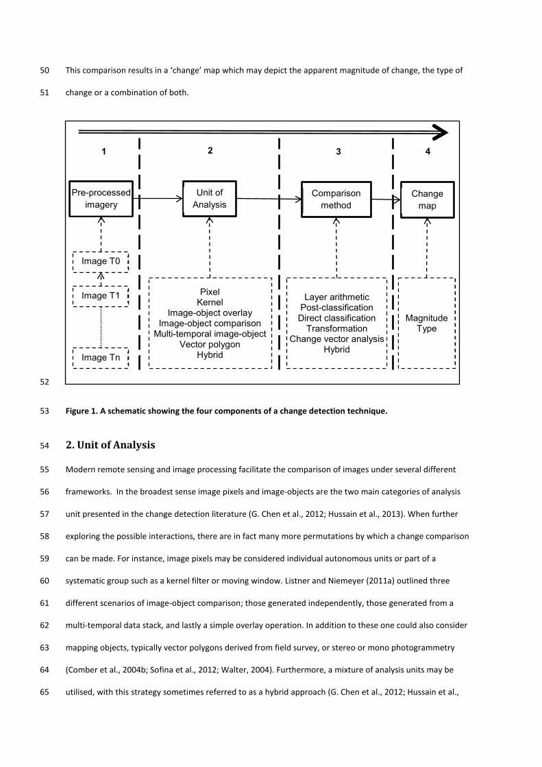
literature. To further clarify these definitions illustrations are given in Figure 2, where the absolute change 69

magnitude under each unit of analysis is depicted for a bi-temporal pair of images. The review then continues 70

with a more detailed discussion of each unit of analysis. 71

Table 1: An overview of analysis units commonly used in remote sensing change detection studies. The 72 comparable features are based on Avery & Colwell’s fundamental features of image interpretation; as cited 73 by Campbell 1983, p43. 74

Description

Comparable features

Advantages Limitations Example studies

Pixe

l Single image pixels are compared.

Tone Shadow (limited)

Fast and suitable for larger pixels sizes. The unit does not generalise the data.

May be unsuitable for higher resolution imagery. Tone is

the only comparable reference point.

Abd El-Kawy et al. (2011); Deng et al. (2008); Green et al.,

(1994); Hame et al., (1998); Jensen & Toll, (1982); Ochoa-Gaona & Gonzalez-Espinosa

(2000); Peiman (2011); Rahman et al. (2011); Shalaby & Tateishi (2007); Torres-Vera

et al. (2009)

Kern

el Groups of pixels are

compared within a kernel filter or moving

window.

Tone Texture

Pattern (limited) Association (limited)

Shadow (limited)

Enables measures of statistical correlation and texture. Facilitates basic

contextual measures.

Generalises the data. The scale of the comparison is typically limited by a fixed

kernel size. Adaptive kernels have been developed but

multi-scale analysis remains a challenge. Contextual information is limited.

Bruzzone & Prieto (2000); He et al. (2011); Im & Jensen (2005); Klaric et al. (2013); Volpi et al.

(2013)

Imag

e-ob

ject

ove

rlay

Image-objects are generated by

segmenting one of the images in the time

series. A comparison against other images is then made by simple

overlay.

Tone Texture

Pattern (limited) Association (limited)

Shadow (limited)

Segmentation may provide a more meaningful framework

for texture measures and generalisation. Provides a

suitable framework for modelling contextual

features.

Generalises the data. Object size and shape cannot be

compared. Sub-object change may remain undetectable.

Comber et al. (2004a); Listner & Niemeyer (2011a);

Tewkesbury & Allitt (2010); Tewkesbury (2011)

Imag

e-ob

ject

co

mpa

rison

Image-objects are generated by

segmenting each image in the time

series independently.

Tone Texture

Size Shape

Pattern Association

Shadow

Shares the advantages of image-object overlay plus an

independent spatial framework facilitates rigorous comparisons.

Generalises the data. Linking image-objects over time is a

challenge. Inconsistent segmentation

leads to object ‘slivers’.

Boldt et al. (2012); Dingle Robertson & King (2011);

Ehlers et al. (2006); Gamanya et al. (2009); Listner &

Niemeyer (2011a); Lizarazo (2012)

Mul

ti-te

mpo

ral

imag

e-ob

ject

Image-objects are generated by

segmenting the entire time series together.

Tone Texture Pattern

Association Shadow

Shares the advantages of image-object overlay plus

the segmentation can honour both static and

dynamic boundaries while maintaining a consistent

topology.

Generalises the data. Object size and shape cannot be

compared.

Bontemps et al. (2012); Chehata et al. (2011); Desclée

et al. (2006); Doxani et al. (2011); Teo & Shih (2013)

Vect

or p

olyg

on

Vector polygons extracted from digital mapping or cadastral

datasets.

Tone Texture

Association Shadow (limited)

Digital mapping databases often provide a

cartographically ‘clean’ basis for analysis with the

potential to focus the analysis using attributed

thematic information.

Generalises the data. Object size and shape cannot be

compared.

Comber et al. (2004b); Duro et al. (2013); Gerard et al. (2010);

Sofina et al. (2012); Walter (2004)

Hyb

rid Segmented image-

objects generated from a pixel or kernel level

comparison.

Tone Texture Pattern

Association Shadow

The level of generalisation may be chosen with

reference to the identified radiometric change.

Although size and shape cannot be used in the

comparison it may be used in the interpretation of the

radiometric change.

Object size and shape cannot be compared.

Aguirre-Gutiérrez et al. (2012); Bazi et al. (2010); Bruzzone &

Bovolo (2013)

75

Image 1 Change magnitude Image 2

Pixel

Kernel (moving window)

Image-object overlay

Image-object comparison

Multi-temporal image-object

Vector polygon

Hybrid

Figure 2. A matrix of analysis units commonly used in remote sensing change detection studies. Image 1 is 76 25cm resolution aerial imagery over Norwich, UK from 2006. Image 2 is aerial imagery captured over the 77 same area in 2010, also at 25cm resolution. The change magnitude is the absolute difference between Image 78 1 and Image 2 calculated over the respective unit of analysis. All imagery ©Airbus Defence and Space Ltd. 79 2014. 80

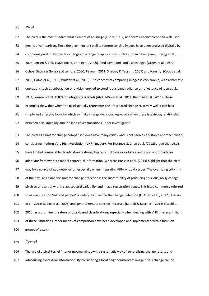
Pixel 81

The pixel is the most fundamental element of an image (Fisher, 1997) and forms a convenient and well used 82

means of comparison. Since the beginning of satellite remote sensing images have been analysed digitally by 83

comparing pixel intensities for changes in a range of applications such as urban development (Deng et al., 84

2008; Jensen & Toll, 1982; Torres-Vera et al., 2009), land cover and land use changes (Green et al., 1994; 85

Ochoa-Gaona & Gonzalez-Espinosa, 2000; Peiman, 2011; Shalaby & Tateishi, 2007) and forestry (Coops et al., 86

2010; Hame et al., 1998; Wulder et al., 2008). The concept of comparing images is very simple, with arithmetic 87

operations such as subtraction or division applied to continuous band radiance or reflectance (Green et al., 88

1994; Jensen & Toll, 1982), or integer class labels (Abd El-Kawy et al., 2011; Rahman et al., 2011). These 89

examples show that when the pixel spatially represents the anticipated change relatively well it can be a 90

simple and effective focus by which to make change decisions, especially when there is a strong relationship 91

between pixel intensity and the land cover transitions under investigation. 92

The pixel as a unit for change comparison does have many critics, and is not seen as a suitable approach when 93

considering modern Very High Resolution (VHR) imagery. For instance G. Chen et al. (2012) argue that pixels 94

have limited comparable classification features, typically just tone or radiance and so do not provide an 95

adequate framework to model contextual information. Whereas Hussain et al. (2013) highlight that the pixel 96

may be a source of geometric error, especially when integrating different data types. The overriding criticism 97

of the pixel as an analysis unit for change detection is the susceptibility of producing spurious, noisy change 98

pixels as a result of within class spectral variability and image registration issues. This issue commonly referred 99

to as classification ‘salt and pepper’ is widely discussed in the change detection (G. Chen et al., 2012; Hussain 100

et al., 2013; Radke et al., 2005) and general remote sensing literature (Baraldi & Boschetti, 2012; Blaschke, 101

2010) as a prominent feature of pixel-based classifications, especially when dealing with VHR imagery. In light 102

of these limitations, other means of comparison have been developed and implemented with a focus on 103

groups of pixels. 104

Kernel 105

The use of a pixel kernel filter or moving window is a systematic way of generalising change results and 106

introducing contextual information. By considering a local neighbourhood of image pixels change can be 107

interpreted statistically, aiming to filter noise and identify ‘true’ change. A neighbourhood of pixels is also a 108

means of modelling local texture and contextual relationships by statistical and knowledge-based means. For 109

instance, Im & Jensen (2005) used a neighbourhood correlation analysis to improve the identification of 110

change information in VHR imagery by considering linear regression parameters instead of pixel radiance 111

alone. The use of kernel-based texture measures have also proved to be a complementary addition to the 112

change detection problem in several studies including those by He et al. (2011) & Klaric et al. (2013). 113

Furthermore, the use of contextual information is an effective method of filtering spurious change pixels 114

(Bruzzone & Prieto, 2000; Volpi et al., 2013). These examples highlight the benefit of kernel filters; as a means 115

of reducing spurious change and as a mechanism of allowing change decisions to be made beyond basic tonal 116

differences. Unfortunately, kernel filters are often operated at a fixed scale and the determination of optimum 117

window sizes is not clearly defined (Warner, 2011). Consequently their use can lead to blurred boundaries and 118

the removal of smaller features. 119

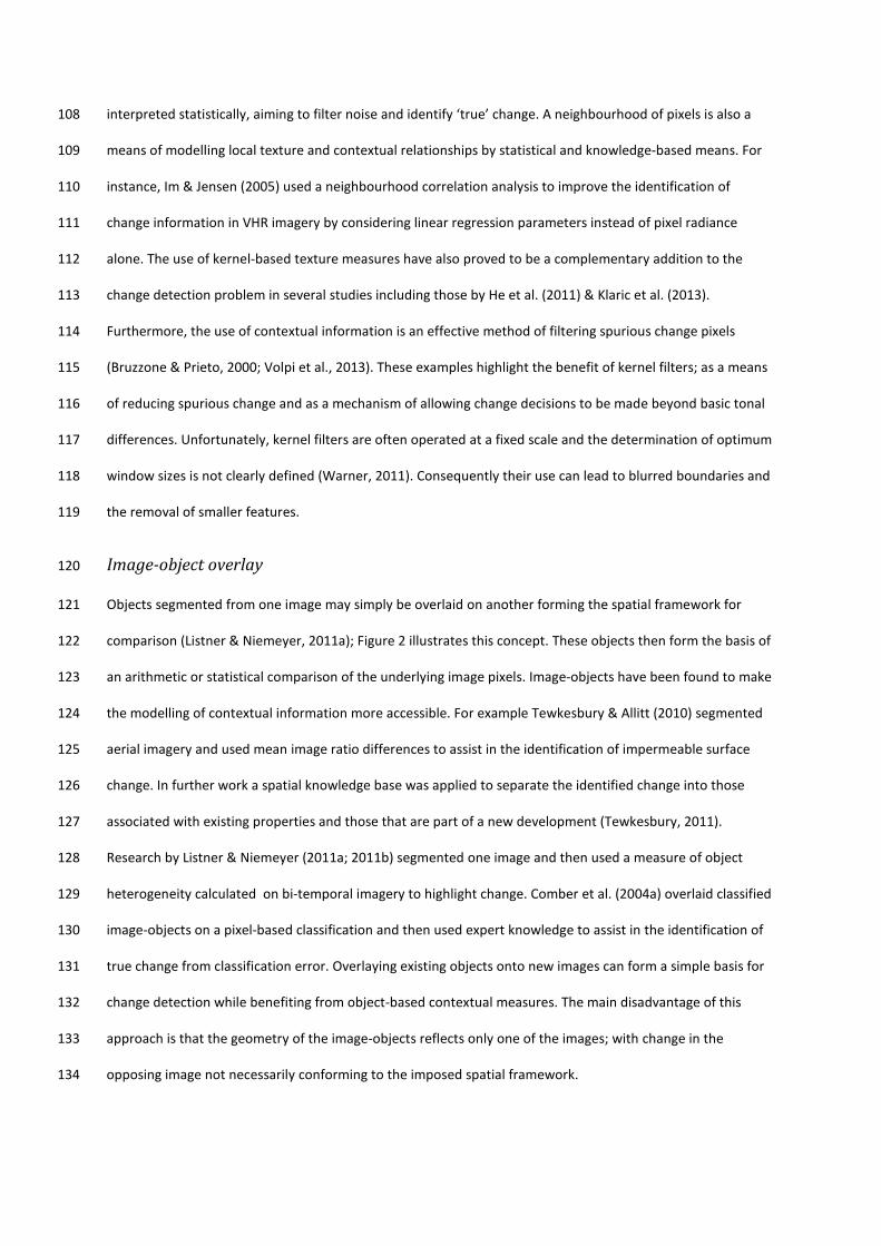
Image-object overlay 120

Objects segmented from one image may simply be overlaid on another forming the spatial framework for 121

comparison (Listner & Niemeyer, 2011a); Figure 2 illustrates this concept. These objects then form the basis of 122

an arithmetic or statistical comparison of the underlying image pixels. Image-objects have been found to make 123

the modelling of contextual information more accessible. For example Tewkesbury & Allitt (2010) segmented 124

aerial imagery and used mean image ratio differences to assist in the identification of impermeable surface 125

change. In further work a spatial knowledge base was applied to separate the identified change into those 126

associated with existing properties and those that are part of a new development (Tewkesbury, 2011). 127

Research by Listner & Niemeyer (2011a; 2011b) segmented one image and then used a measure of object 128

heterogeneity calculated on bi-temporal imagery to highlight change. Comber et al. (2004a) overlaid classified 129

image-objects on a pixel-based classification and then used expert knowledge to assist in the identification of 130

true change from classification error. Overlaying existing objects onto new images can form a simple basis for 131

change detection while benefiting from object-based contextual measures. The main disadvantage of this 132

approach is that the geometry of the image-objects reflects only one of the images; with change in the 133

opposing image not necessarily conforming to the imposed spatial framework. 134

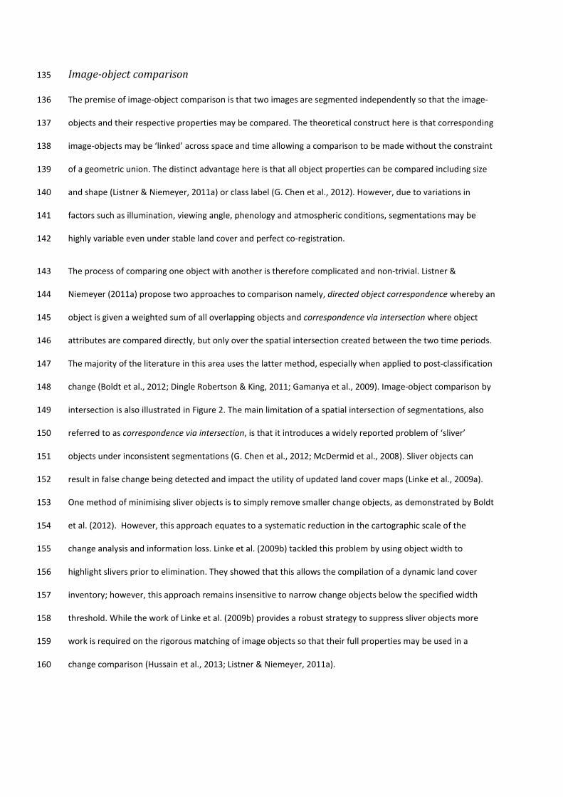
Image-object comparison 135

The premise of image-object comparison is that two images are segmented independently so that the image-136

objects and their respective properties may be compared. The theoretical construct here is that corresponding 137

image-objects may be ‘linked’ across space and time allowing a comparison to be made without the constraint 138

of a geometric union. The distinct advantage here is that all object properties can be compared including size 139

and shape (Listner & Niemeyer, 2011a) or class label (G. Chen et al., 2012). However, due to variations in 140

factors such as illumination, viewing angle, phenology and atmospheric conditions, segmentations may be 141

highly variable even under stable land cover and perfect co-registration. 142

The process of comparing one object with another is therefore complicated and non-trivial. Listner & 143

Niemeyer (2011a) propose two approaches to comparison namely, directed object correspondence whereby an 144

object is given a weighted sum of all overlapping objects and correspondence via intersection where object 145

attributes are compared directly, but only over the spatial intersection created between the two time periods. 146

The majority of the literature in this area uses the latter method, especially when applied to post-classification 147

change (Boldt et al., 2012; Dingle Robertson & King, 2011; Gamanya et al., 2009). Image-object comparison by 148

intersection is also illustrated in Figure 2. The main limitation of a spatial intersection of segmentations, also 149

referred to as correspondence via intersection, is that it introduces a widely reported problem of ‘sliver’ 150

objects under inconsistent segmentations (G. Chen et al., 2012; McDermid et al., 2008). Sliver objects can 151

result in false change being detected and impact the utility of updated land cover maps (Linke et al., 2009a). 152

One method of minimising sliver objects is to simply remove smaller change objects, as demonstrated by Boldt 153

et al. (2012). However, this approach equates to a systematic reduction in the cartographic scale of the 154

change analysis and information loss. Linke et al. (2009b) tackled this problem by using object width to 155

highlight slivers prior to elimination. They showed that this allows the compilation of a dynamic land cover 156

inventory; however, this approach remains insensitive to narrow change objects below the specified width 157

threshold. While the work of Linke et al. (2009b) provides a robust strategy to suppress sliver objects more 158

work is required on the rigorous matching of image objects so that their full properties may be used in a 159

change comparison (Hussain et al., 2013; Listner & Niemeyer, 2011a). 160

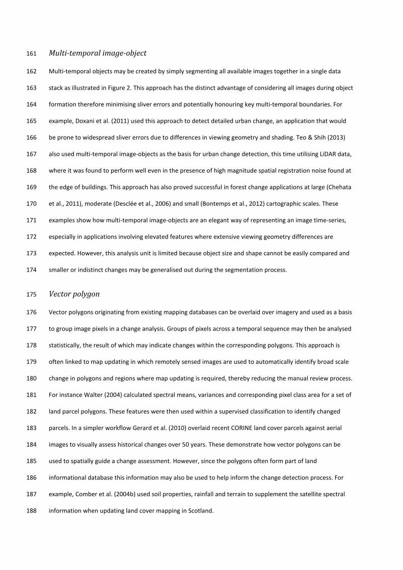
Multi-temporal image-object 161

Multi-temporal objects may be created by simply segmenting all available images together in a single data 162

stack as illustrated in Figure 2. This approach has the distinct advantage of considering all images during object 163

formation therefore minimising sliver errors and potentially honouring key multi-temporal boundaries. For 164

example, Doxani et al. (2011) used this approach to detect detailed urban change, an application that would 165

be prone to widespread sliver errors due to differences in viewing geometry and shading. Teo & Shih (2013) 166

also used multi-temporal image-objects as the basis for urban change detection, this time utilising LiDAR data, 167

where it was found to perform well even in the presence of high magnitude spatial registration noise found at 168

the edge of buildings. This approach has also proved successful in forest change applications at large (Chehata 169

et al., 2011), moderate (Desclée et al., 2006) and small (Bontemps et al., 2012) cartographic scales. These 170

examples show how multi-temporal image-objects are an elegant way of representing an image time-series, 171

especially in applications involving elevated features where extensive viewing geometry differences are 172

expected. However, this analysis unit is limited because object size and shape cannot be easily compared and 173

smaller or indistinct changes may be generalised out during the segmentation process. 174

Vector polygon 175

Vector polygons originating from existing mapping databases can be overlaid over imagery and used as a basis 176

to group image pixels in a change analysis. Groups of pixels across a temporal sequence may then be analysed 177

statistically, the result of which may indicate changes within the corresponding polygons. This approach is 178

often linked to map updating in which remotely sensed images are used to automatically identify broad scale 179

change in polygons and regions where map updating is required, thereby reducing the manual review process. 180

For instance Walter (2004) calculated spectral means, variances and corresponding pixel class area for a set of 181

land parcel polygons. These features were then used within a supervised classification to identify changed 182

parcels. In a simpler workflow Gerard et al. (2010) overlaid recent CORINE land cover parcels against aerial 183

images to visually assess historical changes over 50 years. These demonstrate how vector polygons can be 184

used to spatially guide a change assessment. However, since the polygons often form part of land 185

informational database this information may also be used to help inform the change detection process. For 186

example, Comber et al. (2004b) used soil properties, rainfall and terrain to supplement the satellite spectral 187

information when updating land cover mapping in Scotland. 188

Existing class labels can provide useful information in change detection workflows, allowing efforts to be 189

focused and acting as a thematic guide for classification algorithms. For instance, Bouziani et al. (2010) & 190

Sofina et al. (2012) used a ‘map guided’ approach to train a supervised classification algorithm to identify new 191

buildings and Duro et al. (2013) used cross correlation analysis to statistically identify change candidates based 192

on existing land cover map class labels. The use of vector polygons as a framework for change detection has 193

great potential especially in cases where existing, high quality attribution is used to inform the classification 194

process. However, an assumption of this approach is that the scale of the vector polygons matches the scale of 195

the change of interest. If this is not the case then a strategy will need to be considered to adequately represent 196

the change; for instance pixels may be used to delineate smaller change features within a vector polygon. 197

Hybrid 198

A hybrid approach refers to a combination of analysis units to highlight change in a stepwise way. In its most 199

basic form this relates to a change comparison of pixels which are then filtered or segmented as a mechanism 200

to interpret what the change image is showing. For example, Bazi et al. (2010) first derived a pixel-based 201

change image and then used multi-resolution segmentation to logically group the results. Their approach 202

proved successful when experimentally applied to Landsat and Ikonos imagery. Figure 2 replicates the method 203

employed by Bazi et al. (2010), first calculating the absolute difference between image pixels and then 204

performs a multi-resolution segmentation on the difference image before finally calculating the mean absolute 205

difference of the original images by image-object. Research by Linke et al. (2009b) found that a multi-206

resolution segmentation of pixel-based Landsat wetness difference images proved an effective method of 207

identifying montane land cover change in Alberta, Canada. Aguirre-Gutiérrez et al. (2012) combined pixel and 208

object-based classifications in a post-classification workflow that sought to retain the most accurate elements 209

of each. Bruzzone & Bovolo (2013) modelled different elements of change at the pixel level to include 210

shadows, registration noise and change magnitude. These pixel-based change indicators were then used to 211

inform a change classification based on overriding multi-temporal image-objects. These examples show that 212

using a hybrid of analysis units may be an intuitive approach whereby change in pixel intensity is logically 213

grouped towards identifying features of interest. 214

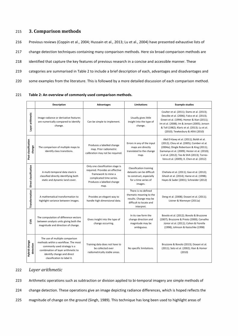
3. Comparison methods 215

Previous reviews (Coppin et al., 2004; Hussain et al., 2013; Lu et al., 2004) have presented exhaustive lists of 216

change detection techniques containing many comparison methods. Here six broad comparison methods are 217

identified that capture the key features of previous research in a concise and accessible manner. These 218

categories are summarised in Table 2 to include a brief description of each, advantages and disadvantages and 219

some examples from the literature. This is followed by a more detailed discussion of each comparison method. 220

Table 2: An overview of commonly used comparison methods. 221

Description Advantages Limitations Example studies

Laye

r arit

hmet

ic

Image radiance or derivative features are numerically compared to identify

change. Can be simple to implement.

Usually gives little insight into the type of

change.

Coulter et al. (2011); Dams et al. (2013); Desclée et al. (2006); Falco et al. (2013);

Green et al. (1994); Homer & Xian (2011); Im et al. (2008); Im & Jensen (2005); Jensen

& Toll (1982); Klaric et al. (2013); Lu et al. (2010); Tewkesbury & Allitt (2010)

Post

-cla

ssifi

catio

n ch

ange

The comparison of multiple maps to identify class transitions.

Produces a labelled change map. Prior radiometric

calibration may not be required.

Errors in any of the input maps are directly

translated to the change map.

Abd El-Kawy et al. (2011); Boldt et al. (2012); Chou et al. (2005); Comber et al. (2004a); Dingle Robertson & King (2011);

Gamanya et al. (2009); Hester et al. (2010); Li et al. (2012); Teo & Shih (2013); Torres-

Vera et al. (2009); X. Chen et al. (2012)

Dire

ct c

lass

ifica

tion

A multi-temporal data stack is classified directly identifying both

static and dynamic land cover.

Only one classification stage is required. Provides an effective

framework to mine a complicated time series.

Produces a labelled change map.

Classification training datasets can be difficult to construct, especially

for a time series of images.

Chehata et al. (2011); Gao et al. (2012); Ghosh et al. (2014); Hame et al. (1998); Hayes & Sader (2001); Schneider (2012)

Tran

sfor

mat

ion

A mathematical transformation to highlight variance between images.

Provides an elegant way to handle high dimensional data.

There is no defined thematic meaning to the results. Change may be difficult to locate and

interpret.

Deng et al. (2008); Doxani et al. (2011); Listner & Niemeyer (2011a)

CVA

The computation of difference vectors between analysis units giving both the

magnitude and direction of change.

Gives insight into the type of change occurring.

In its raw form the change direction and

magnitude may be ambiguous.

Bovolo et al. (2012); Bovolo & Bruzzone (2007); Bruzzone & Prieto (2000); Carvalho

Júnior et al. (2011); Cohen & Fiorella (1998); Johnson & Kasischke (1998)

Hyb

rid c

hang

e de

tect

ion

The use of multiple comparison methods within a workflow. The most

commonly used strategy is a combination of layer arithmetic to

identify change and direct classification to label it.

Training data does not have to be collected over

radiometrically stable areas. No specific limitations.

Bruzzone & Bovolo (2013); Doxani et al. (2011); Seto et al. (2002); Xian & Homer

(2010)

Layer arithmetic 222

Arithmetic operations such as subtraction or division applied to bi-temporal imagery are simple methods of 223

change detection. These operations give an image depicting radiance differences, which is hoped reflects the 224

magnitude of change on the ground (Singh, 1989). This technique has long been used to highlight areas of 225

image change quickly with minimal supervision (Green et al., 1994; Jensen & Toll, 1982) and is still in use 226

today, typically applied to image-objects (Desclée et al., 2006; Tewkesbury & Allitt, 2010). To add thematic 227

meaning to a difference image, the image radiance may be transformed into a vegetation index or fractional 228

cover image prior to the layer arithmetic. For example Coulter et al. (2011) differenced regionally normalised 229

measures of NDVI to identify vegetative land cover change while Tewkesbury & Allitt (2010) used image ratios 230

to identify vegetation removal in aerial imagery. It is also common to monitor urban expansion by subtracting 231

multi-temporal impermeable surface fractional cover images obtained by sub-pixel analysis (Dams et al., 2013; 232

Gangkofner et al., 2010; Lu et al.,2010). A highly evolved system of layer differencing is presented by Jin et al. 233

(2013), whereby change is assessed based upon combining difference images of image spectral indices and 234

biophysical transformations. These examples demonstrate how simple arithmetic operations of image 235

radiance, or derivative features can be used to highlight changed areas, target specific features based upon an 236

expected spectral response or quantify fractional, sub-pixel changes. 237

Layer arithmetic comparisons may go beyond simple radiometric differencing by leveraging different units of 238

analysis. This empowers the comparison by considering texture, context and morphology; therefore reducing 239

the dependency on a target’s spectral characteristics as an indicator of change. For instance Im & Jensen 240

(2005) found that measures of kernel similarity –namely correlation coefficient, slope and offset- proved to be 241

more effective indicators of change than simple pixel differencing. Further work showed that this same 242

comparison method may also be applied to multi-temporal image-objects (Im et al., 2008); although no 243

significant improvement was found when compared to the kernel based approach. When working with VHR 244

imagery several researchers have incorporated measures of texture and morphology into the arithmetic 245

comparison as a means of reducing the dependence on image tone. For instance, Klaric et al. (2013) present a 246

change detection system based on a weighted combination of neighbourhood spectral, textural and 247

morphological features. The authors argue that this approach is not entirely dependent on spectral change and 248

is applicable to multi-spectral and panchromatic imagery. The idea of reducing the dependence on spectral 249

information is further developed by Falco et al. (2013) in research using Quickbird panchromatic imagery 250

alone, as a basis for change detection, by comparing measures of morphology and spatial autocorrelation. 251

Image change isn’t necessarily associated with a strong spectral difference, and these examples have shown 252

how researchers have tackled this problem by using contextual information. However, there is still much 253

research to be done in this area to improve classification accuracies over complex targets. 254

Post-classification change 255

Post-classification change or map-to-map change detection is the process of overlaying coincident thematic 256

maps from different time periods to identify changes between them. The distinct advantage of this technique 257

is that the baseline classification and the change transitions are explicitly known. Furthermore, since the maps 258

may be produced independently, a radiometric normalisation is not necessary (Coppin et al., 2004; Warner et 259

al., 2009). The direct comparison of satellite derived land cover maps is one of the most established and widely 260

used change detection methods, applicable to Landsat class imagery (Abd El-Kawy et al., 2011; Dingle 261

Robertson & King, 2011; Gamanya et al., 2009; Torres-Vera et al., 2009) and VHR imagery (Boldt et al., 2012; 262

Demir et al., 2013; Hester et al., 2010). The approach may also be used to locate changes of a specific 263

thematic target. For instance, Boldt et al. (2012) and Teo & Shih (2013) both used post-classification change to 264

uniquely identify building changes. These examples show that post-classification change is a thematically rich 265

technique able to answer specific change questions, making it suitable for a range of different applications. 266

Post-classification change is limited by map production issues and compounded errors making it a costly and 267

difficult method to adopt. The comparison method requires the production of two entire maps which may be 268

an expensive (Lu et al., 2004) and an operationally complex task. Furthermore, input maps may be produced 269

using differing data and algorithms. In this case, a distinction must be made between classification 270

inconsistencies and real change as explored by Comber et al. (2004a). The biggest issue with post-classification 271

change is that it is entirely dependent on the quality of the input maps (Coppin et al., 2004; Lu et al., 2004) 272

with individual errors compounding in the change map (Serra et al., 2003). Therefore, it is difficult and 273

expensive to produce a time series of maps with sufficient quality to obtain meaningful change results. 274

There have been significant efforts to improve post-classification change results by accounting for classification 275

uncertainty and by modelling anticipated change scenarios. Classification uncertainty may be spatial, thematic 276

or a combination of both and accounted for by assigning confidences to these criteria. For instance, X. Chen et 277

al. (2012) compared fuzzy class probability, rather than crisp labels, to highlight uncertain land cover 278

transitions. Hester et al. (2010) used spatial and thematic fuzziness in the classification of urban change using 279

Quickbird imagery accounting for increased pixel level mis-registration in VHR imagery. Specific change 280

scenarios can also be modelled in an attempt to identify and remove unlikely land cover transitions. For 281

instance Chou et al. (2005) developed a spatial knowledge base, implemented as pixel kernel filters to remove 282

change pixels not conforming to pre-determined change scenarios. This approach has also been extended to 283

include full urban simulations as a means of identifying unlikely transitions (Li et al., 2012). These examples 284

demonstrate that post-classification change has been extended from a simple map label arithmetic operation 285

to one that considers the confidence of a particular label and the likelihood of its indicated change. 286

Direct classification 287

A multi-temporal stack of images can be directly classified to give a land cover inventory over stable areas and 288

land cover transitions where change has occurred. The data stack consists of multiple sets of n band images 289

which may be treated by a classifier as one set of classification features. This is then classified with a 290

supervised or unsupervised technique aiming to give a set of stable land cover classes and changed land cover 291

transitions. The technique is advantageous, since only one classification stage is required and identified 292

changes are thematically labelled. Several researchers investigating forest change have used this approach as a 293

means of directly identifying their target of interest. For instance, Hayes & Sader (2001), Hame et al. (1998) 294

and Chehata et al. (2011) all implemented forest change detection systems based an unsupervised 295

classification of multi-temporal imagery, facilitated by a good understanding of the nature of the change. 296

These examples from forestry applications show how the direct classification technique can be used to solve a 297

relatively well constrained problem. However, direct classification is a powerful tool in the context of a data 298

mining problem such as the interpretation of a dense time series of images. Such a scenario is very difficult to 299

conceptualise or model with expert knowledge, and is an ideal scenario for machine learning algorithms. For 300

example, Schneider (2012) was able to successfully mine a time series of 50 Landsat images from 1988 to 2010 301

for changes in urban extent using supervised support vector machine (SVM) and decision tree classifiers. The 302

dense time series and machine learning approach allowed the extraction of meaningful change under 303

complicated phenological patterns without explicitly modelling them. Gao et al. (2012) also used this strategy, 304

applying a supervised decision tree classifier to extract impermeable surface change over 33 years using nine 305

Landsat images. These examples demonstrate that the direct classification of a time series of images can be an 306

effective way of deciphering change that may be buried within complex patterns. However, deriving training 307

datasets for such a classification can be very challenging (Lu et al., 2004) and unsupervised approaches can 308

prove unresponsive to small magnitude change patterns (Warner et al., 2009). In light of these limitations, 309

recent work by Ghosh et al. (2014) into semi-supervised change classification is extremely interesting with 310

more research needed in this area. 311

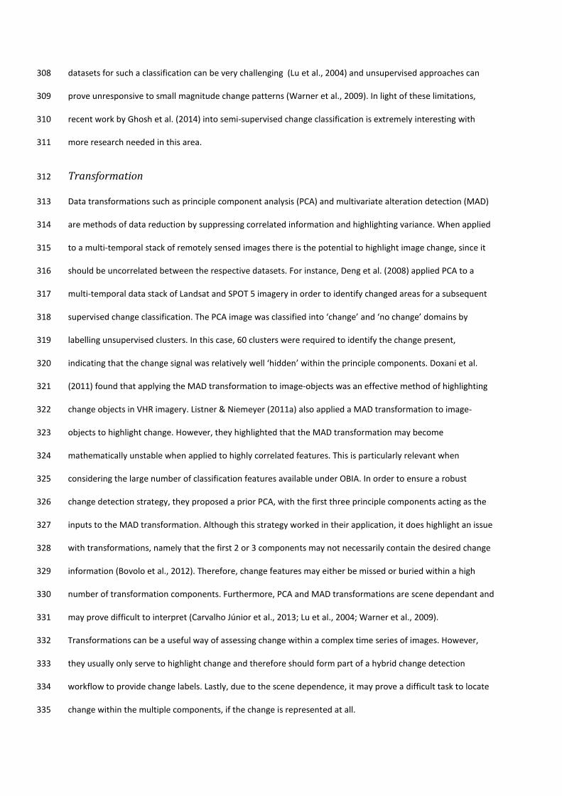
Transformation 312

Data transformations such as principle component analysis (PCA) and multivariate alteration detection (MAD) 313

are methods of data reduction by suppressing correlated information and highlighting variance. When applied 314

to a multi-temporal stack of remotely sensed images there is the potential to highlight image change, since it 315

should be uncorrelated between the respective datasets. For instance, Deng et al. (2008) applied PCA to a 316

multi-temporal data stack of Landsat and SPOT 5 imagery in order to identify changed areas for a subsequent 317

supervised change classification. The PCA image was classified into ‘change’ and ‘no change’ domains by 318

labelling unsupervised clusters. In this case, 60 clusters were required to identify the change present, 319

indicating that the change signal was relatively well ‘hidden’ within the principle components. Doxani et al. 320

(2011) found that applying the MAD transformation to image-objects was an effective method of highlighting 321

change objects in VHR imagery. Listner & Niemeyer (2011a) also applied a MAD transformation to image-322

objects to highlight change. However, they highlighted that the MAD transformation may become 323

mathematically unstable when applied to highly correlated features. This is particularly relevant when 324

considering the large number of classification features available under OBIA. In order to ensure a robust 325

change detection strategy, they proposed a prior PCA, with the first three principle components acting as the 326

inputs to the MAD transformation. Although this strategy worked in their application, it does highlight an issue 327

with transformations, namely that the first 2 or 3 components may not necessarily contain the desired change 328

information (Bovolo et al., 2012). Therefore, change features may either be missed or buried within a high 329

number of transformation components. Furthermore, PCA and MAD transformations are scene dependant and 330

may prove difficult to interpret (Carvalho Júnior et al., 2013; Lu et al., 2004; Warner et al., 2009). 331

Transformations can be a useful way of assessing change within a complex time series of images. However, 332

they usually only serve to highlight change and therefore should form part of a hybrid change detection 333

workflow to provide change labels. Lastly, due to the scene dependence, it may prove a difficult task to locate 334

change within the multiple components, if the change is represented at all. 335

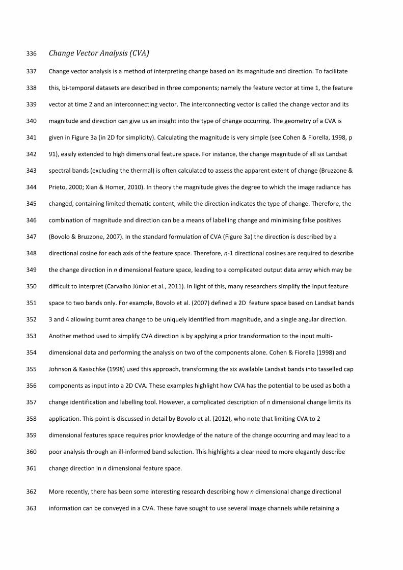
Change Vector Analysis (CVA) 336

Change vector analysis is a method of interpreting change based on its magnitude and direction. To facilitate 337

this, bi-temporal datasets are described in three components; namely the feature vector at time 1, the feature 338

vector at time 2 and an interconnecting vector. The interconnecting vector is called the change vector and its 339

magnitude and direction can give us an insight into the type of change occurring. The geometry of a CVA is 340

given in Figure 3a (in 2D for simplicity). Calculating the magnitude is very simple (see Cohen & Fiorella, 1998, p 341

91), easily extended to high dimensional feature space. For instance, the change magnitude of all six Landsat 342

spectral bands (excluding the thermal) is often calculated to assess the apparent extent of change (Bruzzone & 343

Prieto, 2000; Xian & Homer, 2010). In theory the magnitude gives the degree to which the image radiance has 344

changed, containing limited thematic content, while the direction indicates the type of change. Therefore, the 345

combination of magnitude and direction can be a means of labelling change and minimising false positives 346

(Bovolo & Bruzzone, 2007). In the standard formulation of CVA (Figure 3a) the direction is described by a 347

directional cosine for each axis of the feature space. Therefore, n-1 directional cosines are required to describe 348

the change direction in n dimensional feature space, leading to a complicated output data array which may be 349

difficult to interpret (Carvalho Júnior et al., 2011). In light of this, many researchers simplify the input feature 350

space to two bands only. For example, Bovolo et al. (2007) defined a 2D feature space based on Landsat bands 351

3 and 4 allowing burnt area change to be uniquely identified from magnitude, and a single angular direction. 352

Another method used to simplify CVA direction is by applying a prior transformation to the input multi-353

dimensional data and performing the analysis on two of the components alone. Cohen & Fiorella (1998) and 354

Johnson & Kasischke (1998) used this approach, transforming the six available Landsat bands into tasselled cap 355

components as input into a 2D CVA. These examples highlight how CVA has the potential to be used as both a 356

change identification and labelling tool. However, a complicated description of n dimensional change limits its 357

application. This point is discussed in detail by Bovolo et al. (2012), who note that limiting CVA to 2 358

dimensional features space requires prior knowledge of the nature of the change occurring and may lead to a 359

poor analysis through an ill-informed band selection. This highlights a clear need to more elegantly describe 360

change direction in n dimensional feature space. 361

More recently, there has been some interesting research describing how n dimensional change directional 362

information can be conveyed in a CVA. These have sought to use several image channels while retaining a 363

simple description of the change direction. For instance, Carvalho Júnior et al. (2011) proposed the use of the 364

spectral angle mapper (SAM) and its statistically normalised derivative, spectral correlation mapper (SCM), 365

both well-established techniques, common in hyperspectral remote sensing. Such techniques are used to 366

describe how similar any two n dimensional vectors are to each other, and so has clear applicability to change 367

detection. SAM, mathematically based on the inner product of two vectors (Yuan et al., 1998) is the single 368

angle between two n dimensional vectors (Figure 3b). It is worth re-iterating that SAM and SCM are both 369

measures of similarity and do not give change direction or type per-se. However, they can be highly 370

informative and complementary to a change vector analysis (Carvalho Júnior et al., 2011). 371

The principle behind SAM was further explored by Bovolo et al. (2012) in order to relate the single angle back 372

to change direction. This work used the same theoretical basis as Carvalho Júnior et al. (2011) but instead 373

evaluated the angle between the change vector itself and an arbitrary reference vector (Figure 3c), and Bovolo 374

et al. (2012) normalised the reference vector by setting all elements equal to √𝑛 𝑛� . The rationale for this 375

approach is that the use of an arbitrary reference vector gives a consistent baseline for the change direction, 376

allowing thematic changes to be consistently grouped throughout a scene. Bovolo et al. (2012) argue with 377

reference to experimental examples, that this formulation of CVA does not require any prior knowledge of the 378

anticipated change or its remote sensing response. Moreover, the technique can identify more types of change 379

since all of the available information is considered. These developments could go some way towards 380

establishing CVA as a universal framework for change detection as suggested by Johnson & Kasischke (1998). 381

Due to the recent nature of this research there are few published examples however the underlying 382

philosophy has great potential, particularly when considering future super spectral satellite missions and the 383

wide variety of object-based features available. At the time of writing there is no published research 384

integrating the work of Carvalho Júnior et al. (2011) and Bovolo et al. (2012), despite the complementary 385

nature of these descriptors of multi-dimensional change. 386

A little-reported limitation of CVA is that both the magnitude and direction can be ambiguous (Johnson & 387

Kasischke, 1998). Consider the three identified formulations of CVA displayed in Figure 3a, b & c. It is evident 388

that the change vector itself can be translated within the feature space, while retaining the same measures of 389

magnitude and direction. There is the possibility that multiple thematic changes may be described by identical 390

measures of magnitude and direction, limiting the power of CVA as a change labelling tool. In appraising this 391

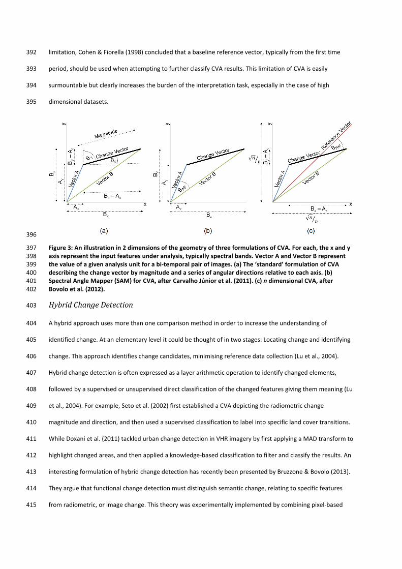
limitation, Cohen & Fiorella (1998) concluded that a baseline reference vector, typically from the first time 392

period, should be used when attempting to further classify CVA results. This limitation of CVA is easily 393

surmountable but clearly increases the burden of the interpretation task, especially in the case of high 394

dimensional datasets. 395

396

Figure 3: An illustration in 2 dimensions of the geometry of three formulations of CVA. For each, the x and y 397 axis represent the input features under analysis, typically spectral bands. Vector A and Vector B represent 398 the value of a given analysis unit for a bi-temporal pair of images. (a) The ‘standard’ formulation of CVA 399 describing the change vector by magnitude and a series of angular directions relative to each axis. (b) 400 Spectral Angle Mapper (SAM) for CVA, after Carvalho Júnior et al. (2011). (c) n dimensional CVA, after 401 Bovolo et al. (2012). 402

Hybrid Change Detection 403

A hybrid approach uses more than one comparison method in order to increase the understanding of 404

identified change. At an elementary level it could be thought of in two stages: Locating change and identifying 405

change. This approach identifies change candidates, minimising reference data collection (Lu et al., 2004). 406

Hybrid change detection is often expressed as a layer arithmetic operation to identify changed elements, 407

followed by a supervised or unsupervised direct classification of the changed features giving them meaning (Lu 408

et al., 2004). For example, Seto et al. (2002) first established a CVA depicting the radiometric change 409

magnitude and direction, and then used a supervised classification to label into specific land cover transitions. 410

While Doxani et al. (2011) tackled urban change detection in VHR imagery by first applying a MAD transform to 411

highlight changed areas, and then applied a knowledge-based classification to filter and classify the results. An 412

interesting formulation of hybrid change detection has recently been presented by Bruzzone & Bovolo (2013). 413

They argue that functional change detection must distinguish semantic change, relating to specific features 414

from radiometric, or image change. This theory was experimentally implemented by combining pixel-based 415

measures of shadow, radiometric change and noise within an object-based classification. These examples 416

highlight a trend amongst research that seeks to use multiple stages of change comparison to solve particular 417

problems, a trend which is likely to continue as workflows become ever more complex. 418

4. Discussion 419

Here, we consider some of the specific issues which underlie this review, and make some practical suggestions 420

which may be adopted in future experimental and applied research. The organisation and nomenclature 421

developed is a response to the burgeoning change detection literature, proliferated by the addition of object-422

based methods. While OBCD has undoubted merits, the pixel as an analysis unit and allied comparison 423

methods are still very relevant. Therefore, remotely sensed optical image change detection should be 424

considered as a whole. We further discuss this rationale starting with the recent rise of OBCD and why its use 425

should be carefully considered on merit and better-organised in experimental research. We then discuss an 426

application-driven framework to identify requirements, and inform the selection of an appropriate unit of 427

analysis and comparison method based on scale and thematic objectives. We argue that a unit of analysis 428

should be selected based on its representation of the application scale with respect to the available image 429

resolution, and its ability to deliver the required comparison features. On the other hand the comparison 430

method must fit the application’s thematic objectives. 431

There is currently a debate in the remote sensing literature over the merits of object-based change detection 432

(OBCD) verses traditional pixel-based methods. Some believe that OBCD is a more advanced solution, capable 433

of producing more accurate estimates of change particularly when VHR imagery is used. For instance G Chen 434

et al. (2012) and Hussain et al. (2013) argue that OBCD is an advancement beyond pixel-based change 435

detection that generates fewer spurious results with an enhanced capability to model contextual information. 436

Moreover, Boldt et al. (2012) describe pixel-based change detection of VHR imagery as inappropriate. Kuntz et 437

al. (2011) comments that objects are less sensitive to geometric errors due to a greater potential for a majority 438

overlap and Im et al. (2008) points to the fact that OBIA may be a more efficient means of making change 439

comparisons. Crucially, objects are described as an intuitive vehicle to apply expert knowledge (Blaschke, 440

2010; Vieira et al., 2012) which if operationalized would represent an opportunity to model specific change 441

features. 442

There is a significant technical overlap between object and pixel-based approaches. It is becoming increasing 443

common in the literature to subdivide change detection methods into either pixel or object-based approaches 444

followed by a range of sub-methods (Boldt et al., 2012; G. Chen et al., 2012; Hussain et al., 2013). This results 445

in a very disparate and complicated set of change detection methods, making evaluation and selection 446

extremely difficult. However, many of the sub-methods are very similar, if not identical, varying only by the 447

analysis unit used for the comparison. For instance, post-classification change remains conceptually the same 448

under pixel and object-based implementations as shown in a comparative analysis by Walter (2004). Simple 449

arithmetic change operations such as differencing and ratios (Green et al., 1994; Jensen & Toll, 1982) -arguably 450

the foundation of remote sensing change detection- may be applied equally to pixels or image-objects. More 451

complicated procedures such as a multivariate correlation analysis may also be applied to pixels or objects (Im 452

et al., 2008). Warner et al. (2009) suggests that any change detection technique that can be applied to pixels 453

can also be applied to objects. While there are obvious merits to working with objects, it is not always useful to 454

make a hard distinction between object and pixel-based change detection. This can result in an overly 455

complicated and disparate presentation of the available techniques. 456

Focusing on OBCD may unnecessarily narrow the focus of a literature review or method selection because of a 457

bias towards the unit of analysis, at the detriment of the comparison methodology. Although using image-458

objects for change analysis has its undoubted merits and is a ‘hot topic’ for research (Blaschke, 2010), it is 459

important to consider remote sensing change detection as a whole and be aware of advancements in both 460

pixel and object-based methods since they are usually interchangeable. For instance, two recent reviews of 461

change detection focusing on OBIA methods (G. Chen et al., 2012; Hussain et al., 2013) bypass recent 462

important advancements in CVA (Bovolo & Bruzzone, 2007; Bovolo et al., 2012; Carvalho Júnior et al., 2011). 463

CVA and the vast majority of comparison methodologies are not constrained to image pixels with a change 464

analysis executable on pixels, primitive image-objects or meaningful image-objects (Bruzzone & Bovolo, 2013). 465

In essence, change detection workflows are more often than not transferable between analysis units 466

regardless of their initial conception. Ultimately, it is more useful to make a technique selection considering 467

the merits of both the comparison methodology and analysis unit in relation to the task in hand. 468

OBIA and by association OBCD is a means of generalising image pixels, with the segmentation scale directly 469

controlling the size of detectable features. When segmenting at a particular scale the resultant objects are 470

conveying statistical summaries of the underlying pixels. As highlighted by Walter (2004), regions of change 471

must occupy a significant proportion of an object or exhibit extraordinary magnitude in order to be detectable. 472

Therefore, the segmentation scale and image resolution must be carefully chosen so as to adequately define 473

change features of interest (Hall & Hay, 2003). Dingle Robertson & King (2011) highlight that the selection of 474

an appropriate segmentation scale is not straightforward. In their workflow they qualitatively identified a 475

suitable segmentation scale but nonetheless found that smaller, less abundant classes were not retained in 476

their post-classification change analysis. The generalising properties of OBIA are however actively used as a 477

means of removing spurious, ‘salt and pepper’ features (Boldt et al., 2012; Im et al., 2008). This point would be 478

of particular concern when seeking change at large cartographic scales. Clearly then, when considering an 479

object-based unit of analysis, the size of the target change must be known prior to performing the analysis so 480

that a suitable segmentation scale may be applied. 481

Experimental methods aiming to test object-based methods against pixel-based counterparts are often flawed 482

because several variables are under comparison. Research aiming to compare pixel-based classifications 483

against object-based ones should then be designed with the analysis unit as the sole variable. Under the 484

framework presented in this review, change detection analysis units could then be meaningfully compared 485

while maintaining identical comparison methodologies. However, it is often the case that experiments are 486

undertaken varying both the analysis unit and comparison or classification method. For instance, Dingle 487

Robertson & King (2011) compared a maximum likelihood classification of pixels to a nearest neighbour 488

classification of image-objects; While Myint et al. (2011) compared nearest neighbour and knowledge based 489

classifications of image-objects to a maximum likelihood pixel classification. These experiments provide 490

conclusions based on compounded variables with the effect of an analysis unit change confused with a change 491

of classification algorithm. Conversely, interesting research by Duro et al. (2012) found that the differences in 492

accuracy of pixel and object-based classifications were not statistically significant when executed with the 493

same machine learning algorithm. There is then a case for caution before declaring object-based methods as 494

superior. In the case of change detection it is hoped that the clearer demarcation between the analysis unit 495

and comparison methodology presented in this review can help to steer research in this area, providing more 496

reliable information as to the relative merits of each component. 497

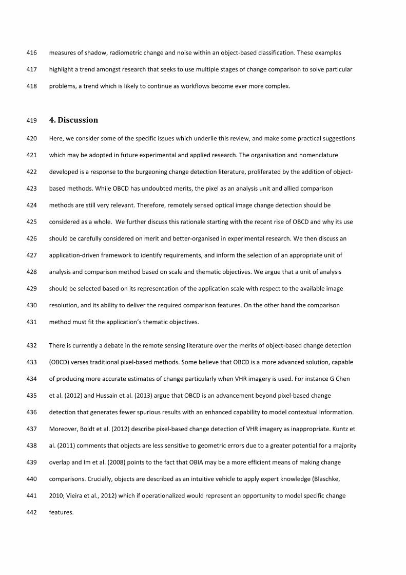
The nomenclature presented here may be used to help guide method selection in applied research. While this 498

is an extremely complicated and non-prescriptive task, we believe that the breakdown of change detection 499

into two discrete components does help to focus selection decisions more meaningfully. An application-driven 500

framework is provided by which to build criteria for a technique selection. This framework, along with the key 501

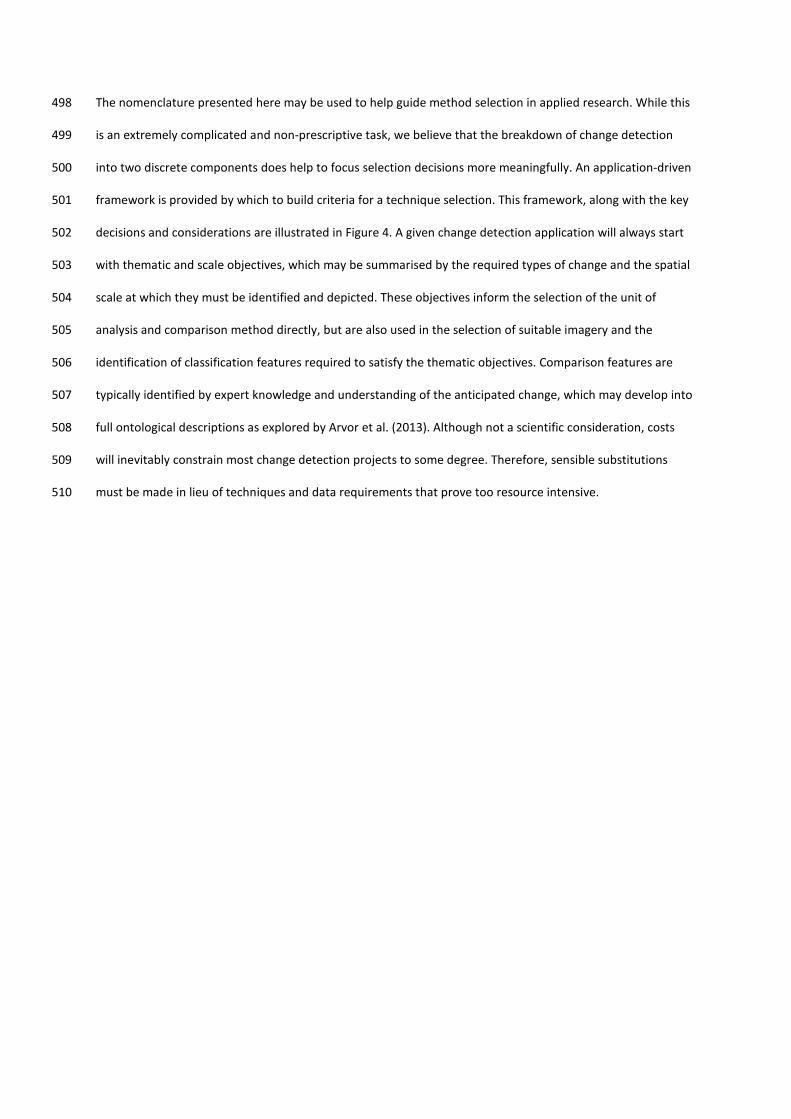
decisions and considerations are illustrated in Figure 4. A given change detection application will always start 502

with thematic and scale objectives, which may be summarised by the required types of change and the spatial 503

scale at which they must be identified and depicted. These objectives inform the selection of the unit of 504

analysis and comparison method directly, but are also used in the selection of suitable imagery and the 505

identification of classification features required to satisfy the thematic objectives. Comparison features are 506

typically identified by expert knowledge and understanding of the anticipated change, which may develop into 507

full ontological descriptions as explored by Arvor et al. (2013). Although not a scientific consideration, costs 508

will inevitably constrain most change detection projects to some degree. Therefore, sensible substitutions 509

must be made in lieu of techniques and data requirements that prove too resource intensive. 510

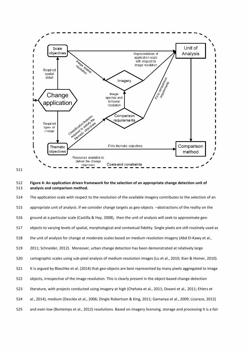
511

Figure 4: An application driven framework for the selection of an appropriate change detection unit of 512 analysis and comparison method. 513

The application scale with respect to the resolution of the available imagery contributes to the selection of an 514

appropriate unit of analysis. If we consider change targets as geo-objects –abstractions of the reality on the 515

ground at a particular scale (Castilla & Hay, 2008), then the unit of analysis will seek to approximate geo-516

objects to varying levels of spatial, morphological and contextual fidelity. Single pixels are still routinely used as 517

the unit of analysis for change at moderate scales based on medium resolution imagery (Abd El-Kawy et al., 518

2011; Schneider, 2012). Moreover, urban change detection has been demonstrated at relatively large 519

cartographic scales using sub-pixel analysis of medium resolution images (Lu et al., 2010; Xian & Homer, 2010). 520

It is argued by Blaschke et al. (2014) that geo-objects are best represented by many pixels aggregated to image 521

objects, irrespective of the image resolution. This is clearly present in the object-based change detection 522

literature, with projects conducted using imagery at high (Chehata et al., 2011; Doxani et al., 2011; Ehlers et 523

al., 2014), medium (Desclée et al., 2006; Dingle Robertson & King, 2011; Gamanya et al., 2009; Lizarazo, 2012) 524

and even low (Bontemps et al., 2012) resolutions. Based on imagery licensing, storage and processing it is a fair 525

assumption that the cost to conduct a change analysis will be related to the number of pixels under 526

investigation. Therefore, the use of aggregated image-object units of analysis may represent a higher cost 527

solution for a given application scale. For example, the sub-pixel detection of change at a relatively large 528

cartographic scale employed by Xian & Homer (2010) presents a solution with ‘reasonable costs and 529

production times’ (Xian & Homer, 2010, p1685). Given the huge variability present in the literature, it is not 530

possible to recommend an appropriate unit of analysis based on the application scale and image resolution 531

alone. Clearly, cost has influenced previous projects but the required comparable features, driven by an 532

application’s thematic objectives is a crucial factor that completes the decision. 533

The classification features required to make a meaningful change comparison are pivotal when selecting an 534

appropriate unit of analysis. To illustrate this point, we consider the comparisons requirements for a specific 535

change application, (the comparison of impervious surfaces) and then refer to instances in the literature that 536

have addressed this problem. The comprehensive identification of impervious surfaces, and the monitoring of 537

their change over time using remotely sensed data, would require the comparison of multi-spectral image 538

tone, supplemented by texture and context. More specifically, this task might involve the analysis of: (1) Key 539

absorption and reflection features present in the visible, near-infrared and especially short-wave infrared 540

regions (Weng, 2012), (2) Fine scale textures (Perry & Nawaz, 2008), and lastly (3) The image scene’s 541

contextual and 3D parameters (Herold, 2008). Interpreting these may imply an image-object comparison of 542

hyperspectral imagery; which may be beyond the resources of most applications. Therefore, it is common to 543

sensibly reduce the scope of a change analysis to meet the available resources. For example, while Landsat 544

imagery does not have the spectral fidelity to model impervious spectral responses precisely, Landsat’s broad 545

short wave infrared band is useful in the task. For example, Xian & Homer (2010) developed a sub-pixel 546

method of estimating relatively large-scale impervious surface change derived from the spectral information of 547

30m Landsat pixels alone. If there is an exploitable spectral signature associated with the change of interest, 548

which may be identified in the available data, then a tonal comparison only is required. This opens up all 549

available units of analysis. For instance, forest change has been detected by comparing image tone by pixel 550

(Cohen & Fiorella, 1998; Hayes & Sader, 2001; Tan et al., 2013), image-object overlay (Tian et al., 2013) or 551

multi-temporal image-objects (Bontemps et al., 2012). Returning to the impervious surface change theme, 552

Zhou, et al. (2008) found that their available VHR colour infrared images were insufficient to detect impervious 553

surfaces spectrally. Therefore, 3D LiDAR information and auxiliary mapping was utilised to assist with the 554

detection. Research by X. Chen et al. (2012) also found spectral confusion in change detection, this time 555

between forest and cropland change. In these circumstances, the inclusion of additional classification features 556

-facilitated by units of analysis other than the pixel- may be used to improve change detection results. For 557

example, kernel based texture (He et al., 2011), multi-temporal image-object texture (Desclée et al., 2006), 558

image-object shape comparison (Boldt et al., 2012), local image correlation from kernel (Im & Jensen, 2005) 559

and multi-temporal image-objects (Im et al., 2008) and lastly, context modelled with kernels (Volpi et al., 2013) 560

and image-object comparison (Hazel, 2001). To summarise, if the target of interest is associated with a 561

measurable spectral signature then the separation may be ‘trivial’ (Blaschke et al., 2014, p182), opening up all 562

available units of analysis. In this case selection may be based on the application’s scale objectives and the 563

available imagery. For more complex situations, the ability of the unit of analysis to model textural, 564

morphological and contextual features over time should be used in the selection. Image-object comparison 565

presents the most comprehensive framework, but the technical complications may limit its application. 566

Therefore in such circumstances, image-object comparison and hybrid approaches offer simplified, albeit more 567

limited frameworks. 568

The thematic objectives of an application must be carefully considered when evaluating a comparison method. 569

Consequently, it is important to distinguish between the two broad outcomes of a change analysis, namely the 570

identification of radiometric change and semantic change (Bruzzone & Bovolo, 2013). Radiometric change 571

relates to spectral or image change (Warner et al., 2009) and is simply an observed difference in image tone. 572

Radiometric change relates to all changes indiscriminately to include actual changes on the ground and those 573

associated with illumination, phenology or viewing geometry. Semantic change on the other hand is 574

thematically subdivided into meaningful categories – be they differences in scene shading or specific land 575

cover transitions. Clearly, semantic change is of greater value, directly informing the end user. Unfortunately, 576

these two very different outcomes are normally presented jointly as ‘change detection’ (Johnson & Kasischke, 577

1998) making comparisons between different research projects very difficult. Generally, simple layer 578

arithmetic comparisons resulting in a difference image depict radiometric change only, leaving the end user to 579

review all radiometric change prior to identifying features of interest. Bruzzone & Bovolo (2013) have argued 580

strongly that change detection should identify different types of change in order to effectively remove noise 581

and isolate targets of interest. The default choice of identifying semantic change for applications requiring 582

meaningful, quantitative information is post-classification change (Abd El-Kawy et al., 2011; Rahman et al., 583

2011; Torres-Vera et al., 2009) but this may be prohibitively expensive in some cases. In applications such as 584

impervious surface change (Lu et al., 2010), layer arithmetic may be used to directly inform the thematic 585

objectives. For more complicated requirements, a direct classification of a multi-temporal data stack shows 586

great potential, especially when applied to a dense time series with suitable training data. 587

5. Conclusions 588

This review has presented optical image change detection techniques to a clear, succinct nomenclature based 589

on the unit of analysis and the comparison methodology. This nomenclature significantly reduces conceptual 590

overlap in modern change detection making a synoptic view of the field far more accessible. Furthermore, this 591

approach will help to guide technique comparison research by placing a clear separation of variables between 592

the analysis unit and classification method. 593

The summary of analysis units shows that more research is required to identify optimum approaches for 594

change detection. While image-object comparison is theoretically the most powerful unit, in light of 595

inconsistent segmentations, matching image-objects over space and time requires far more sophisticated map 596

conflation technology. Therefore, multi-temporal image-objects or a hybrid approach are likely the most 597

robust analysis units, while the pixel is still suitable for many applications. It is recommended that future 598

research in this area ensures a strict separation of analysis unit and comparison method variables in order to 599

provide clearer information on the relative merits of each. 600

Post-classification change is the most popular comparison method due to the descriptive nature of the results 601

allowing specific thematic questions to be answered. A direct classification of a complicated data stack is also 602

an effective method of identifying semantic changes. However, the required training data is extremely difficult 603

to obtain since the location of change is usually not known prior to an analysis. As highlighted by Lu et al. 604

(2004) a hybrid approach may inherit the benefits of a direct classification while simplifying training data 605

collection. Recent developments in CVA provide a powerful framework to compare multi-dimensional data but 606

remain largely untested in the literature. Therefore, more research is required exploring recent formulations of 607

CVA, in particularly the effect of integrating object-based features and other contextual measures. 608

The use of image-objects as the unit of analysis in a change detection workflow should be a carefully 609

considered decision based on the application at hand rather than adopted as a default choice. The main factor 610

in this decision should be the requirement to compare features inherent to image-objects such as morphology 611

and context. This decision must also include the scale of the analysis and acceptable levels of generalisation to 612

be applied with respect to the pixel size of the images under analysis. 613

Remote sensing change detection is a vast subject that has evolved significantly in the last 30 years but more 614

research is required to tackle persistent problems. These include: scene illumination effects (Hussain et al., 615

2013; Singh, 1989), changes in viewing geometry (Listner & Niemeyer, 2011a; Lu et al., 2004), scale and the 616

identification of small, ‘sub-area’ change (G. Chen et al., 2012), objects based feature utilisation (G. Chen et al., 617

2012; Hussain et al., 2013) and segmentation consistency and comparison (Hussain et al., 2013; Listner & 618

Niemeyer, 2011a). This review makes a contribution by offering a clearer organisation by which to conduct 619

research in this field. 620

Acknowledgements 621

Professor Peter Francis Fisher passed away during the preparation of this manuscript and he will be greatly 622

missed. The authors would like to thank the anonymous reviewers for their very useful comments and 623

suggestions that helped to improve the manuscript. This research received no specific grant from any funding 624

agency in the public, commercial, or not-for-profit sectors. 625

References 626

Abd El-Kawy, O. R., Rød, J. K., Ismail, H. A., & Suliman, A. S. (2011). Land use and land cover change detection in 627 the western Nile delta of Egypt using remote sensing data. Applied Geography, 31(2), 483–494. 628 doi:10.1016/j.apgeog.2010.10.012 629

Aguirre-Gutiérrez, J., Seijmonsbergen, A. C., & Duivenvoorden, J. F. (2012). Optimizing land cover classification 630 accuracy for change detection, a combined pixel-based and object-based approach in a mountainous 631 area in Mexico. Applied Geography, 34(5), 29–37. doi:10.1016/j.apgeog.2011.10.010 632

Arvor, D., Durieux, L., Andrés, S., & Laporte, M.-A. (2013). Advances in Geographic Object-Based Image Analysis 633 with ontologies: A review of main contributions and limitations from a remote sensing perspective. ISPRS 634 Journal of Photogrammetry and Remote Sensing, 82, 125–137. doi:10.1016/j.isprsjprs.2013.05.003 635

Atkinson, P. M. (2006). Resolution Manipulation and sub-Pixel Mapping. In S. M. De Jong & F. van der Meer 636 (Eds.), Remote Sensing Image Analysis: Including the Spatial Domain (pp. 51 – 70). Springer. 637

Baraldi, A., & Boschetti, L. (2012). Operational Automatic Remote Sensing Image Understanding Systems: 638 Beyond Geographic Object-Based and Object-Oriented Image Analysis (GEOBIA/GEOOIA). 639 Part 1: Introduction. Remote Sensing, 4(12), 2694–2735. doi:10.3390/rs4092694 640

Bazi, Y., Melgani, F., & Al-Sharari, H. D. (2010). Unsupervised Change Detection in Multispectral Remotely 641 Sensed Imagery With Level Set Methods. IEEE Transactions on Geoscience and Remote Sensing, 48(8), 642 3178–3187. doi:10.1109/TGRS.2010.2045506 643

Blaschke, T. (2010). Object based image analysis for remote sensing. ISPRS Journal of Photogrammetry and 644 Remote Sensing, 65(1), 2–16. doi:10.1016/j.isprsjprs.2009.06.004 645

Blaschke, T., Hay, G. J., Kelly, M., Lang, S., Hofmann, P., Addink, E., … Tiede, D. (2014). Geographic Object-646 Based Image Analysis – Towards a new paradigm. ISPRS Journal of Photogrammetry and Remote Sensing, 647 87, 180–191. doi:10.1016/j.isprsjprs.2013.09.014 648

Boldt, M., Thiele, A., & Schulz, K. (2012). Object-based urban change detection analyzing high resolution 649 optical satellite images. In PROCEEDINGS- SPIE THE INTERNATIONAL SOCIETY FOR OPTICAL 650 ENGINEERING: Earth Resources and Environmental Remote Sensing/GIS Applications III Vol 8538 (p. 651 85380E–1 to 85380E–9). 652

Bontemps, S., Langer, A., & Defourny, P. (2012). Monitoring forest changes in Borneo on a yearly basis by an 653 object-based change detection algorithm using SPOT-VEGETATION time series. International Journal of 654 Remote Sensing, 33(15), 4673–4699. Retrieved from 655 http://www.tandfonline.com/doi/abs/10.1080/01431161.2011.638336 656

Bouziani, M., Goïta, K., & He, D.-C. (2010). Automatic change detection of buildings in urban environment from 657 very high spatial resolution images using existing geodatabase and prior knowledge. ISPRS Journal of 658 Photogrammetry and Remote Sensing, 65(1), 143–153. doi:10.1016/j.isprsjprs.2009.10.002 659

Bovolo, F., & Bruzzone, L. (2007). A theoretical framework for unsupervised change detection based on change 660 vector analysis in the polar domain. IEEE Transactions on Geoscience and Remote Sensing, 45(1), 218–661 236. Retrieved from http://ieeexplore.ieee.org/xpls/abs_all.jsp?arnumber=4039609 662

Bovolo, F., Marchesi, S., & Bruzzone, L. (2012). A framework for automatic and unsupervised detection of 663 multiple changes in multitemporal images. IEEE Transactions on Geoscience and Remote Sensing, 50(6), 664 2196–2212. Retrieved from http://ieeexplore.ieee.org/xpls/abs_all.jsp?arnumber=6085609 665

Bruzzone, L., & Bovolo, F. (2013). A Novel Framework for the Design of Change-Detection Systems for Very-666 High-Resolution Remote Sensing Images. Proceedings of the IEEE, 101(3), 609–630. 667 doi:10.1109/JPROC.2012.2197169 668

Bruzzone, L., & Prieto, D. F. (2000). Automatic analysis of the difference image for unsupervised change 669 detection. IEEE Transactions on Geoscience and Remote Sensing, 38(3), 1171–1182. Retrieved from 670 http://ieeexplore.ieee.org/xpls/abs_all.jsp?arnumber=843009 671

Carvalho Júnior, O. A., Guimarães, R. F., Gillespie, A., Silva, N. C., & Gomes, R. (2011). A New Approach to 672 Change Vector Analysis Using Distance and Similarity Measures. Remote Sensing, 3(12), 2473–2493. 673 doi:10.3390/rs3112473 674

Carvalho Júnior, O. A., Guimarães, R. F., Silva, N. C., Gillespie, A., Gomes, R., Silva, C., & de Carvalho, A. (2013). 675 Radiometric Normalization of Temporal Images Combining Automatic Detection of Pseudo-Invariant 676 Features from the Distance and Similarity Spectral Measures, Density Scatterplot Analysis, and Robust 677 Regression. Remote Sensing, 5(6), 2763–2794. doi:10.3390/rs5062763 678

Castilla, G., & Hay, G. J. (2008). Image objects and geographic objects. In T. Blaschke, S. Lang, & G. J. Hay (Eds.), 679 Object-Based Image Analysis (pp. 91–110). Springer. 680

Chehata, N., Orny, C., Boukir, S., & Guyon, D. (2011). Object-based forest change detection using high 681 resolution satellite images. Remote Sensing and Spatial Information Sciences, 38. Retrieved from 682 http://www.int-arch-photogramm-remote-sens-spatial-inf-sci.net/XXXVIII-3-W22/49/2011/isprsarchives-683 XXXVIII-3-W22-49-2011.pdf 684

Chen, G., Hay, G. J., Carvalho, L. M. T., & Wulder, M. A. (2012). Object-based Change Detection. International 685 Journal of Remote Sensing, 33(14), 4434–4457. Retrieved from 686 http://www.ingentaconnect.com/content/schweiz/pfg/2011/00002011/00000004/art00005 687

Chen, X., Chen, J., Shi, Y., & Yamaguchi, Y. (2012). An automated approach for updating land cover maps based 688 on integrated change detection and classification methods. ISPRS Journal of Photogrammetry and 689 Remote Sensing, 71, 86–95. doi:10.1016/j.isprsjprs.2012.05.006 690

Chou, T. Y., Lei, T. C., Wan, S., & Yang, L. S. (2005). Spatial knowledge databases as applied to the detection of 691 changes in urban land use. International Journal of Remote Sensing, 26(14), 3047–3068. 692 doi:10.1080/01431160500057889 693

Cohen, W. B., & Fiorella, M. (1998). Comparison of Methods for Detecting Conifer Forest Change with 694 Thematic Mapper Imagery. In R. S. Lunetta & C. D. Elvidge (Eds.), Remote Sensing Change Detection (pp. 695 89 – 99). ANN ARBOR PRESS. 696

Comber, A., Fisher, P. F., & Wadsworth, R. (2004a). Assessment of a Semantic Statistical Approach to Detecting 697 Land Cover Change Using Inconsistent Data Sets. Photogrammetric Engineering & Remote Sensing, 70(8), 698 931–938. 699

Comber, A., Law, A. N. R., & Lishman, J. R. (2004b). Application of knowledge for automated land cover change 700 monitoring. International Journal of Remote Sensing, 25(16), 3177–3192. 701 doi:10.1080/01431160310001657795 702

Coops, N. C., Gillanders, S. N., Wulder, M. a., Gergel, S. E., Nelson, T., & Goodwin, N. R. (2010). Assessing 703 changes in forest fragmentation following infestation using time series Landsat imagery. Forest Ecology 704 and Management, 259(12), 2355–2365. doi:10.1016/j.foreco.2010.03.008 705

Coppin, P., Jonckheere, I., Nackaerts, K., Muys, B., & Lambin, E. (2004). Review ArticleDigital change detection 706 methods in ecosystem monitoring: a review. International Journal of Remote Sensing, 25(9), 1565–1596. 707 doi:10.1080/0143116031000101675 708

Coulter, L., Hope, A. S., & Stow, D. A. (2011). Time-space radiometric normalization of TM/ETM+ images for 709 land cover change detection. International Journal of Remote Sensing, 32(20), 7539–3556. Retrieved 710 from http://www.tandfonline.com/doi/abs/10.1080/01431161.2010.524676 711

Dams, J., Dujardin, J., Reggers, R., Bashir, I., Canters, F., & Batelaan, O. (2013). Mapping impervious surface 712 change from remote sensing for hydrological modeling. Journal of Hydrology, 485, 84–95. 713 doi:10.1016/j.jhydrol.2012.09.045 714

Demir, B., Bovolo, F., & Bruzzone, L. (2013). Updating land-cover maps by classification of image time series: A 715 novel change-detection-driven transfer learning approach. IEEE Transactions on Geoscience and Remote 716 Sensing, 51(1), 300–312. Retrieved from http://ieeexplore.ieee.org/xpls/abs_all.jsp?arnumber=6208857 717

Deng, J. S., Wang, K., Deng, Y. H., & Qi, G. J. (2008). PCA-based land-use change detection and analysis using 718 multitemporal and multisensor satellite data. International Journal of Remote Sensing, 29(16), 4823–719 4838. doi:10.1080/01431160801950162 720

Desclée, B., Bogaert, P., & Defourny, P. (2006). Forest change detection by statistical object-based method. 721 Remote Sensing of Environment, 102(1-2), 1–11. doi:10.1016/j.rse.2006.01.013 722

Dingle Robertson, L., & King, D. (2011). Comparison of pixel- and object-based classification in land cover 723 change mapping. International Journal of Remote Sensing, 32(6), 1505–1529. 724 doi:10.1080/01431160903571791 725

Doxani, G., Karantzalos, K., & Tsakiri-Strati, M. (2011). Monitoring urban changes based on scale-space filtering 726 and object-oriented classification. International Journal of Applied Earth Observation and 727 Geoinformation, 15, 38–48. doi:10.1016/j.jag.2011.07.002 728

Duro, D. C., Franklin, S. E., & Dubé, M. G. (2012). A comparison of pixel-based and object-based image analysis 729 with selected machine learning algorithms for the classification of agricultural landscapes using SPOT-5 730 HRG imagery. Remote Sensing of Environment, 118, 259–272. doi:10.1016/j.rse.2011.11.020 731

Duro, D. C., Franklin, S. E., & Dubé, M. G. (2013). Hybrid Object-based Change Detection and Hierarchical 732 Image Segmentation for Thematic Map Updating. Photogrammetric Engineering and Remote Sensing, 733 79(3), 259–268. Retrieved from http://cat.inist.fr/?aModele=afficheN&cpsidt=27040182 734

Ehlers, M., Sofina, N., Filippovska, Y., & Kada, M. (2014). Automated Techniques for Change Detection Using 735 Combined Edge Segment Texture Analysis, GIS, and 3D Information. In Q. Weng (Ed.), Global Urban 736 Monitoring and Assessment through Earth Observation (pp. 325 – 351). CRC Press, Taylor & Francis 737 Group. Retrieved from http://www.crcpress.com/product/isbn/9781466564497 738

Falco, N., Mura, M., & Bovolo, F. (2013). Change Detection in VHR Images Based on Morphological Attribute 739 Profiles. IEEE Geoscience and Remote Sensing Letters, 10(3), 636–640. Retrieved from 740 http://ieeexplore.ieee.org/xpls/abs_all.jsp?arnumber=6374646 741

Fisher, P. F. (1997). The pixel: a snare and a delusion. International Journal of Remote Sensing, 18(3), 679–685. 742 Retrieved from http://www.tandfonline.com/doi/abs/10.1080/014311697219015 743

Gamanya, R., De Maeyer, P., & De Dapper, M. (2009). Object-oriented change detection for the city of Harare, 744 Zimbabwe. Expert Systems with Applications, 36(1), 571–588. doi:10.1016/j.eswa.2007.09.067 745

Gangkofner, U., Weichelsbaum, J., Kuntz, S., Brodksy, L., Larsson, K., & Pasquale, V. D. E. (2010). Update of the 746 European High-resolution Layer of Built-up Areas and Soil Sealing 2006 with Image2009 Data. In 30th 747 EARSeL Symposium: Remote Sensing for Science, Education and Culture. EARSeL. Retrieved from 748 http://www.earsel.org/symposia/2010-symposium-Paris/Proceedings/EARSeL-Symposium-2010_5-749 01.pdf 750

Gao, F., Colstoun, E. de, & Ma, R. (2012). Mapping impervious surface expansion using medium-resolution 751 satellite image time series: a case study in the Yangtze River Delta, China. International Journal of 752 Remote Sensing, 33(24), 7609–7628. Retrieved from 753 http://www.tandfonline.com/doi/abs/10.1080/01431161.2012.700424 754

Gerard, F., Petit, S., Smith, G. M., & Thomson, A. (2010). Land cover change in Europe between 1950 and 2000 755 determined employing aerial photography. Progress in Physical, 34(2), 183–205. 756 doi:10.1177/0309133309360141 757

Ghosh, S., Roy, M., & Ghosh, A. (2014). Semi-supervised change detection using modified self-organizing 758 feature map neural network. Applied Soft Computing, 15, 1–20. doi:10.1016/j.asoc.2013.09.010 759

Green, K., Kempka, D., & Lackey, L. (1994). Using remote sensing to detect and monitor land-cover and land-760 use change. Photogrammetric Engineering & Remote Sensing, 60(3), 331–337. Retrieved from 761 http://cat.inist.fr/?aModele=afficheN&cpsidt=3983194 762

Hall, O., & Hay, G. J. (2003). A Multiscale Object-Specific Approach to Digital Change Detection. International 763 Journal of Applied Earth Observation and Geoinformation, 4(4), 311–327. doi:10.1016/S0303-764 2434(03)00010-2 765

Hame, T., Heiler, I., & San Miguel-Ayanz, J. (1998). An unsupervised change detection and recognition system 766 for forestry. International Journal of Remote Sensing, 19(6), 1079–1099. Retrieved from 767 http://www.tandfonline.com/doi/abs/10.1080/014311698215612 768

Hayes, D., & Sader, S. (2001). Comparison of change-detection techniques for monitoring tropical forest 769 clearing and vegetation regrowth in a time series. Photogrammetric engineering and remote sensing, 770 67(9), 1067–1075. Retrieved from 771 http://www.asprs.org/a/publications/pers/2001journal/september/2001_sep_1067-1075.pdf 772

Hazel, G. G. (2001). Object-level change detection in spectral imagery. IEEE Transactions on Geoscience and 773 Remote Sensing, 39(3), 553–561. Retrieved from 774 http://ieeexplore.ieee.org/xpls/abs_all.jsp?arnumber=911113 775

He, C., Wei, A., Shi, P., Zhang, Q., & Zhao, Y. (2011). Detecting land-use/land-cover change in rural–urban fringe 776 areas using extended change-vector analysis. International Journal of Applied Earth Observation and 777 Geoinformation, 13(4), 572–585. doi:10.1016/j.jag.2011.03.002 778

Herold, M. (2008). Spectral Characteristics of asphalt Road Surfaces. In Q. Weng (Ed.), Remote sensing of 779 impervious surfaces (pp. 237–250). CRC Press, Taylor & Francis Group. 780

Hester, D. B., Nelson, S. A. C., Cakir, H. I., Khorram, S., & Cheshire, H. (2010). High-resolution land cover change 781 detection based on fuzzy uncertainty analysis and change reasoning. International Journal of Remote 782 Sensing, 31(2), 455–475. doi:10.1080/01431160902893493 783

Hussain, M., Chen, D., Cheng, A., Wei, H., & Stanley, D. (2013). Change detection from remotely sensed 784 images: From pixel-based to object-based approaches. ISPRS Journal of Photogrammetry and Remote 785 Sensing, 80, 91–106. doi:10.1016/j.isprsjprs.2013.03.006 786

İlsever, M., & Ünsalan, C. (2012). Two-Dimensional Change Detection Methods (p. 72). Springer. 787

Im, J., & Jensen, J. R. (2005). A change detection model based on neighborhood correlation image analysis and 788 decision tree classification. Remote Sensing of Environment, 99(3), 326–340. 789 doi:10.1016/j.rse.2005.09.008 790

Im, J., Jensen, J. R., & Tullis, J. A. (2008). Object-based change detection using correlation image analysis and 791 image segmentation. International Journal of Remote Sensing, 29(2), 399–423. 792 doi:10.1080/01431160601075582 793

Jensen, J. R., & Toll, D. (1982). Detecting residential land-use development at the urban fringe. 794 Photogrammetric Engineering and Remote Sensing, 48(4), 629–643. Retrieved from 795 http://scholar.google.com/scholar?hl=en&btnG=Search&q=intitle:Detecting+Residential+Land-796 Use+Development+at+the+Urban+Fringe#0 797

Jin, S., Yang, L., Danielson, P., Homer, C., Fry, J., & Xian, G. (2013). A comprehensive change detection method 798 for updating the National Land Cover Database to circa 2011. Remote Sensing of Environment, 132, 159–799 175. doi:10.1016/j.rse.2013.01.012 800

Johnson, R. D., & Kasischke, E. S. (1998). Change vector analysis: A technique for the multispectral monitoring 801 of land cover and condition. International Journal of Remote Sensing, 19(3), 411–426. 802 doi:10.1080/014311698216062 803

Klaric, M. N., Claywell, B. C., Scott, G. J., Hudson, N. J., Sjahputera, O., Li, Y., … Davis, C. H. (2013). GeoCDX: An 804 Automated Change Detection and Exploitation System for High-Resolution Satellite Imagery. IEEE 805 Transactions on Geoscience and Remote Sensing, 51(4), 2067–2086. Retrieved from 806 http://ieeexplore.ieee.org/xpls/abs_all.jsp?arnumber=6479289 807

Kuntz, S., Braun, M., Ernst, C., Gallaun, H., Santos, C., Hame, T., … Kotarba, A. (2011). Geoland 2 - Technical 808 Note - Change Detection Status Report. Retrieved from 809 http://sia.eionet.europa.eu/EAGLE/EAGLE_5rdMeeting_g2_MONINA_FFM/Change Detection Methods-810 I2.pdf 811

Li, X., Zhang, Y., Liu, X., & Chen, Y. (2012). Assimilating process context information of cellular automata into 812 change detection for monitoring land use changes. International Journal of Geographical Information 813 Science, 26(9), 1667–1687. Retrieved from 814 http://www.tandfonline.com/doi/abs/10.1080/13658816.2011.643803 815

Linke, J., McDermid, G. J., Laskin, D. N., McLane, A. J., Pape, A. D., Cranston, J., … Franklin, S. E. (2009b). A 816 Disturbance-Inventory Framework for Flexible and Reliable Landscape Monitoring. Photogrammetric 817 Engineering & Remote Sensing, 75(8), 981–995. doi:10.14358/PERS.75.8.981 818

Linke, J., McDermid, G. J., Pape, A. D., McLane, A. J., Laskin, D. N., Hall-Beyer, M., & Franklin, S. E. (2009a). The 819 influence of patch-delineation mismatches on multi-temporal landscape pattern analysis. Landscape 820 Ecology, 24(2), 157–170. doi:10.1007/s10980-008-9290-z 821

Listner, C., & Niemeyer, I. (2011a). Object-based Change Detection. Photogrammetrie - Fernerkundung - 822 Geoinformation, 2011(4), 233–245. doi:10.1127/1432-8364/2011/0085 823

Listner, C., & Niemeyer, I. (2011b). Recent advances in object-based change detection. In Geoscience and 824 Remote Sensing Symposium (IGARSS), IEEE International (pp. 110–113). Retrieved from 825 http://ieeexplore.ieee.org/xpls/abs_all.jsp?arnumber=6048910 826

Lizarazo, I. (2012). Quantitative land cover change analysis using fuzzy segmentation. International Journal of 827 Applied Earth Observation and Geoinformation, 15, 16–27. doi:10.1016/j.jag.2011.05.012 828

Lu, D., Mausel, P., Brondizio, E. S., & Moran, E. (2004). Change detection techniques. International Journal of 829 Remote Sensing, 25(12), 2365–2401. doi:10.1080/0143116031000139863 830

Lu, D., Moran, E., & Hetrick, S. (2010). Detection of impervious surface change with multitemporal Landsat 831 images in an urban–rural frontier. ISPRS Journal of Photogrammetry and Remote Sensing. 832 doi:10.1016/j.isprsjprs.2010.10.010 833

McDermid, G. J., Linke, J., Pape, A. D., Laskin, D. N., McLane, A. J., & Franklin, S. E. (2008). Object-based 834 approaches to change analysis and thematic map update: challenges and limitations. Canadian Journal of 835 Remote Sensing, 34(5), 462–466. Retrieved from http://www.tandfonline.com/doi/abs/10.5589/m08-836 061 837

Myint, S. W., Gober, P., Brazel, A., Grossman-Clarke, S., & Weng, Q. (2011). Per-pixel vs. object-based 838 classification of urban land cover extraction using high spatial resolution imagery. Remote Sensing of 839 Environment, 115(5), 1145–1161. doi:10.1016/j.rse.2010.12.017 840

Ochoa-Gaona, S., & Gonzalez-Espinosa, M. (2000). Land use and deforestation in the highlands of Chiapas, 841 Mexico. Applied Geography, 20(1), 17–42. doi:10.1016/S0143-6228(99)00017-X 842

Peiman, R. (2011). Pre-classification and post-classification change-detection techniques to monitor land-cover 843 and land-use change using multi-temporal Landsat imagery: a case study. International Journal of 844

Remote Sensing, 32(15), 4365–4381. Retrieved from 845 http://www.tandfonline.com/doi/abs/10.1080/01431161.2010.486806 846

Perry, T., & Nawaz, R. (2008). An investigation into the extent and impacts of hard surfacing of domestic 847 gardens in an area of Leeds, United Kingdom. Landscape and Urban Planning, 86(1), 1–13. 848 doi:10.1016/j.landurbplan.2007.12.004 849

Radke, R. J., Andra, S., Al-Kofahi, O., & Roysam, B. (2005). Image change detection algorithms: a systematic 850 survey. IEEE transactions on image processing, 14(3), 294–307. Retrieved from 851 http://www.ncbi.nlm.nih.gov/pubmed/15762326 852

Rahman, A., Aggarwal, S. P., Netzband, M., & Fazal, S. (2011). Monitoring Urban Sprawl Using Remote Sensing 853 and GIS Techniques of a Fast Growing Urban Centre, India. IEEE Journal of Selected Topics in Applied 854 Earth Observations and Remote Sensing, 4(1), 56–64. 855

Schneider, A. (2012). Monitoring land cover change in urban and peri-urban areas using dense time stacks of 856 Landsat satellite data and a data mining approach. Remote Sensing of Environment, 124, 689–704. 857 doi:10.1016/j.rse.2012.06.006 858

Serra, P., Pons, X., & Sauri, D. (2003). Post-classification change detection with data from different sensors: 859 some accuracy considerations. International Journal of Remote Sensing, 24(16), 3311–3340. Retrieved 860 from http://www.tandfonline.com/doi/abs/10.1080/0143116021000021189 861

Seto, K. C., Woodcock, C. E., Song, C., Huang, X., Lu, J., & Kaufmann, R. K. (2002). Monitoring land-use change 862 in the Pearl River Delta using Landsat TM. International Journal of Remote Sensing, 23(10), 1985–2004. 863 doi:10.1080/01431160110075532 864

Shalaby, A., & Tateishi, R. (2007). Remote sensing and GIS for mapping and monitoring land cover and land-use 865 changes in the Northwestern coastal zone of Egypt. Applied Geography, 27(1), 28–41. 866 doi:10.1016/j.apgeog.2006.09.004 867

Singh, A. (1989). Review Article Digital change detection techniques using remotely-sensed data. International 868 Journal of Remote Sensing, 10(6), 989–1003. doi:10.1080/01431168908903939 869

Sofina, N., Ehlers, M., & Michel, U. (2012). Integrated data processing of remotely sensed and vector data for 870 building change detection. In Proceedings of SPIE The International Society for Optical Enginerring: Earth 871 Resources and Environmental Remote Sensing/GIS Applications III Vol 8538 (p. 85380F–1 to 85380F–8). 872

Tan, B., Masek, J. G., Wolfe, R., Gao, F., Huang, C., Vermote, E. F., … Ederer, G. (2013). Improved forest change 873 detection with terrain illumination corrected Landsat images. Remote Sensing of Environment, 136, 469–874 483. doi:10.1016/j.rse.2013.05.013 875

Teo, T.-A., & Shih, T.-Y. (2013). Lidar-based change detection and change-type determination in urban areas. 876 International Journal of Remote Sensing, 34(3), 968–981. doi:10.1080/01431161.2012.714504 877

Tewkesbury, A. (2011). Mapping the extent of urban creep in Exeter using OBIA. In Proceedings of RSPSoc 878 Annual Conference (p. 163). 879

Tewkesbury, A., & Allitt, M. (2010). Urban creep mapping from Remote Sensing data. In Proceedings of RSPSoc 880 Annual Conference and Irish Earth Observation Symposium (p. 34). 881

Tian, J., Reinartz, P., D’Angelo, P., & Ehlers, M. (2013). Region-based automatic building and forest change 882 detection on Cartosat-1 stereo imagery. ISPRS Journal of Photogrammetry and Remote Sensing, 79, 226–883 239. doi:10.1016/j.isprsjprs.2013.02.017 884

Torres-Vera, M. a., Prol-Ledesma, R. M., & Garcia-Lopez, D. (2009). Three decades of land use variations in 885 Mexico City. International Journal of Remote Sensing, 30(1), 117–138. doi:10.1080/01431160802261163 886

Vieira, M. A., Formaggio, A. R., Rennó, C. D., Atzberger, C., Aguiar, D. A., & Mello, M. P. (2012). Object Based 887 Image Analysis and Data Mining applied to a remotely sensed Landsat time-series to map sugarcane over 888 large areas. Remote Sensing of Environment, 123, 553–562. doi:10.1016/j.rse.2012.04.011 889

Volpi, M., Tuia, D., Bovolo, F., Kanevski, M., & Bruzzone, L. (2013). Supervised change detection in VHR images 890 using contextual information and support vector machines. International Journal of Applied Earth 891 Observation and Geoinformation, 20, 77–85. doi:10.1016/j.jag.2011.10.013 892

Walter, V. (2004). Object-based classification of remote sensing data for change detection. ISPRS Journal of 893 Photogrammetry and Remote Sensing, 58(3-4), 225–238. doi:10.1016/j.isprsjprs.2003.09.007 894

Warner, T. (2011). Kernel-Based Texture in Remote Sensing Image Classification. Geography Compass, 5(10), 895 781–798. doi:10.1111/j.1749-8198.2011.00451.x 896

Warner, T., Almutairi, A., & Lee, J. Y. (2009). Remote Sensing of Land Cover Change. In T. A. Warner, D. M. 897 Nellis, & G. M. Foody (Eds.), The SAGE Handbook of Remote Sensing (pp. 459–472). SAGE Publications. 898

Weng, Q. (2012). Remote sensing of impervious surfaces in the urban areas: Requirements, methods, and 899 trends. Remote Sensing of Environment, 117, 34–49. doi:10.1016/j.rse.2011.02.030 900

Wulder, M. a., Butson, C. R., & White, J. C. (2008). Cross-sensor change detection over a forested landscape: 901 Options to enable continuity of medium spatial resolution measures. Remote Sensing of Environment, 902 112(3), 796–809. doi:10.1016/j.rse.2007.06.013 903

Xian, G., & Homer, C. (2010). Updating the 2001 National Land Cover Database Impervious Surface Products to 904 2006 using Landsat Imagery Change Detection Methods. Remote Sensing of Environment, 114(8), 1676–905 1686. doi:10.1016/j.rse.2010.02.018 906

Yuan, D., Elvidge, C. D., & Lunetta, R. S. (1998). Survey of Multispectral Methods for Land Cover Change 907 Analysis. In R. S. Lunetta & C. D. Elvidge (Eds.), Remote Sensing Change Detection (pp. 21–35). ANN 908 ARBOR PRESS. 909

Zhou, W., Troy, A., & Grove, M. (2008). Object-based land cover classification and change analysis in the 910 Baltimore metropolitan area using multitemporal high resolution remote sensing data. Sensors, 8, 1613–911 1636. Retrieved from http://www.mdpi.com/1424-8220/8/3/1613/htm 912

913