A Credit Scoring Model Based on Classifiers … · A Credit Scoring Model Based on Classifiers...

A Credit Scoring Model Based on Classifiers

Consensus System Approach

A thesis submitted in partial fulfilment of the requirements for the degree

of Doctor of Philosophy (PhD)

Electronic and Computer Engineering

College of Engineering, Design and Physical Sciences

Brunel University London

United Kingdom

by

Maher A. Ala’raj

March 2016

i

ABSTRACT

Managing customer credit is an important issue for each commercial bank; therefore, banks

take great care when dealing with customer loans to avoid any improper decisions that can

lead to loss of opportunity or financial losses. The manual estimation of customer

creditworthiness has become both time- and resource-consuming. Moreover, a manual

approach is subjective (dependable on the bank employee who gives this estimation), which is

why devising and implementing programming models that provide loan estimations is the

only way of eradicating the ‘human factor’ in this problem. This model should give

recommendations to the bank in terms of whether or not a loan should be given, or otherwise

can give a probability in relation to whether the loan will be returned. Nowadays, a number of

models have been designed, but there is no ideal classifier amongst these models since each

gives some percentage of incorrect outputs; this is a critical consideration when each percent

of incorrect answer can mean millions of dollars of losses for large banks. However, the LR

remains the industry standard tool for credit-scoring models development. For this purpose,

an investigation is carried out on the combination of the most efficient classifiers in credit-

scoring scope in an attempt to produce a classifier that exceeds each of its classifiers or

components.

In this work, a fusion model referred to as ‘the Classifiers Consensus Approach’ is

developed, which gives a lot better performance than each of single classifiers that constitute

it. The difference of the consensus approach and the majority of other combiners lie in the

fact that the consensus approach adopts the model of real expert group behaviour during the

process of finding the consensus (aggregate) answer. The consensus model is compared not

only with single classifiers, but also with traditional combiners and a quite complex combiner

model known as the ‘Dynamic Ensemble Selection’ approach.

As a pre-processing technique, step data-filtering (select training entries which fits input data

well and remove outliers and noisy data) and feature selection (remove useless and

statistically insignificant features which values are low correlated with real quality of loan)

are used. These techniques are valuable in significantly improving the consensus approach

results. Results clearly show that the consensus approach is statistically better (with 95%

confidence value, according to Friedman test) than any other single classifier or combiner

ii

analysed; this means that for similar datasets, there is a 95% guarantee that the consensus

approach will outperform all other classifiers. The consensus approach gives not only the best

accuracy, but also better AUC value, Brier score and H-measure for almost all datasets

investigated in this thesis. Moreover, it outperformed Logistic Regression. Thus, it has been

proven that the use of the consensus approach for credit-scoring is justified and

recommended in commercial banks.

Along with the consensus approach, the dynamic ensemble selection approach is analysed,

the results of which show that, under some conditions, the dynamic ensemble selection

approach can rival the consensus approach. The good sides of dynamic ensemble selection

approach include its stability and high accuracy on various datasets.

The consensus approach, which is improved in this work, may be considered in banks that

hold the same characteristics of the datasets used in this work, where utilisation could

decrease the level of mistakenly rejected loans of solvent customers, and the level of

mistakenly accepted loans that are never to be returned. Furthermore, the consensus approach

is a notable step in the direction of building a universal classifier that can fit data with any

structure. Another advantage of the consensus approach is its flexibility; therefore, even if the

input data is changed due to various reasons, the consensus approach can be easily re-trained

and used with the same performance.

iii

DEDICATION

To my lovely parents and family

This thesis is dedicated to my ever-loving mother, Khadija, for her continuous love and

support. She always believed in me and made it all possible. Her endless love and

encouragement has absolutely helped me to achieve my dream. Without her standing by my

side and her permanent support, this work would not have been possible.

To my wonderful father, Abdelhamid, who has been a great source of motivation, inspiration

and everlasting support throughout my journey, and who sacrificed everything for me to be

what I am now.

I also dedicate this work to my wonderful brothers and only sister, Mohammed, Ahmed,

Omar, Ibrahim and Noor, for their incessant love, care and encouragement, also my lovely

nephew Abdelhamid. I owe everything I have achieved or will achieve to my lovely family.

iv

ACKNOWLEDGMENTS

Above all, I am grateful and indebted to almighty God who has given me the strength and

patience to complete this work and who remains to bless me every day.

First of all, I am deeply beholden to my thesis supervisor, Dr. Maysam Abbod, whom he is

the base of this work. I thank him for his valuable guidance, encouragement, and enduring

support during this journey. He has always been there when I have needed him, and his

advice has made a huge contribution to my academic and personal development.

I want to take the chance like to express my deepest thanks and gratitude to all those who

have helped me and offered their support over these past years of my PhD journey. Also

special thanks goes to my best friends Dr. Tamer Darwish, Dr. Mohammed Radi and Dr. Ziad

Hunaiti whom they were a real support to me and faithful friends during this journey.

v

DECLARATION

It is hereby declared that the thesis in focus is the author’s own work and is submitted for the

first time to the Post-Graduate Research Office. The study was originated, composed and

reviewed by the mentioned author and supervisors in the Department of Electronic and

Computer Engineering, College of Engineering, Design and Physical Sciences, Brunel

University London UK. All the information derived from other works has been properly

referenced and acknowledged.

Maher A. Ala’raj

March 2016

London, UK

vi

TABLE OF CONTENTS

Abstract .................................................................................................................................................................. i

Dedication ............................................................................................................................................................. iii

Acknowledgments ................................................................................................................................................ iv

Declaration ............................................................................................................................................................ v

Table of Contents ................................................................................................................................................. vi

List of Figures ...................................................................................................................................................... xi

List of Tables ...................................................................................................................................................... xiv

List of Abbreviations ........................................................................................................................................ xvii

Chapter 1 ............................................................................................................................................................... 1

Introduction .......................................................................................................................................................... 1

1.1 Background.......................................................................................................................................... 1

1.2 Research Motivations .......................................................................................................................... 2

1.3 Aim and Objectives ............................................................................................................................. 3

1.4 Contributions to Knowledge .............................................................................................................. 4

1.5 Structure of the Thesis ........................................................................................................................ 4

1.6 List of Publications .............................................................................................................................. 6

CHAPTER 2 .......................................................................................................................................................... 7

Background and Review of the Literature ......................................................................................................... 7

2.1 Introduction ......................................................................................................................................... 7

2.2 What is Credit-Scoring ....................................................................................................................... 7

2.2.1 The Importance of Credit-Scoring ................................................................................ 10

2.2.2 Credit-Scoring Evaluation Techniques ......................................................................... 11

2.2.2.1 Judgmental Scoring Systems ........................................................................................ 12

2.2.2.2 Credit-Scoring Systems................................................................................................. 13

2.3 Quantitative Credit-Scoring ............................................................................................................. 14

2.3.1 LDA .............................................................................................................................. 15

2.3.2 LR ................................................................................................................................. 16

2.3.3 DT ................................................................................................................................. 18

2.3.4 NB ................................................................................................................................. 20

2.3.5 MARS ........................................................................................................................... 21

2.3.6 NN ................................................................................................................................. 23

2.3.7 SVM .............................................................................................................................. 25

2.3.8 RF .................................................................................................................................. 26

2.4 Credit-Scoring Modelling Approaches ............................................................................................ 28

vii

2.4.1 Individual Classifiers .................................................................................................... 28

2.4.2 Hybrid Techniques ........................................................................................................ 29

2.4.3 Ensemble Techniques ................................................................................................... 30

2.5 Model Performance and Significance Measures ............................................................................ 32

2.6 Credit-scoring Studies ...................................................................................................................... 33

2.6.1 Literature Review Collection Process ........................................................................... 34

2.6.2 Literature Discussion and Analysis ............................................................................... 35

2.7 Summary ............................................................................................................................................ 45

Chapter 3 ............................................................................................................................................................. 47

The Experimental Design Framework for the Proposed Credit-scoring Model ........................................... 47

3.1 Introduction ....................................................................................................................................... 47

3.2 Datasets .............................................................................................................................................. 47

3.2.1 Dataset Size ................................................................................................................... 47

3.2.2 Number of Datasets ....................................................................................................... 48

3.2.3 Collection of the Datasets ............................................................................................. 49

3.3 Data Pre-Processing .......................................................................................................................... 50

3.3.1 Data Imputation............................................................................................................. 51

3.3.2 Data Normalisation ....................................................................................................... 52

3.3.4 Data-filtering (Instance Selection) ................................................................................ 54

3.4 Data Splitting and Partitioning Techniques.................................................................................... 55

3.4.1 Holdout Technique ........................................................................................................ 56

3.4.2 K-Fold Cross-validation ................................................................................................ 57

3.5 Modelling Approach ......................................................................................................................... 58

3.6 Performance Evaluation Measurement ........................................................................................... 59

3.6.1 Confusion Matrix Measures .......................................................................................... 59

3.6.1.1 Accuracy Rate ............................................................................................................... 60

3.6.1.2 Sensitivity and Specificity ............................................................................................ 60

3.6.1.3 Type I and II Error ........................................................................................................ 61

3.6.2 Area Under the Curve ................................................................................................... 61

3.6.3 H-Measure ..................................................................................................................... 63

3.6.4 Brier Score .................................................................................................................... 63

3.7 Statistical Tests of Significance ........................................................................................................ 64

3.8 The Proposed Experimental Design Framework ........................................................................... 66

3.9 Summary ............................................................................................................................................ 66

Chapter 4 ............................................................................................................................................................. 68

Credit-Scoring Models using Individual Classifiers Techniques .................................................................... 68

4.1 Introduction ....................................................................................................................................... 68

viii

4.2 Individual Classifiers Development ................................................................................................. 69

4.2.1 Data Pre-processing and Preparation for Training and Evaluation ............................... 69

4.2.2 Classifiers Parameters Selection and Tuning ................................................................ 69

4.3 Experimental Results ........................................................................................................................ 72

4.4 Analysis and Discussion .................................................................................................................... 85

4.5 Summary ............................................................................................................................................ 88

Chapter 5 ............................................................................................................................................................. 90

Credit-Scoring Models Using Hybrid Classifiers Techniques ........................................................................ 90

5.1 Introduction ....................................................................................................................................... 90

5.2 Data-Filtering .................................................................................................................................... 91

5.2.1 Classifiers Results Using the GNG filtering algorithm ................................................. 97

5.3 Feature Selection ............................................................................................................................. 100

5.3.1 Classifiers Results Using MARS ................................................................................ 105

5.4 Classifiers Results Using GNG + MARS ....................................................................................... 108

5.5 Comparison of Results and Justification of Combining GNG + MARS .................................... 119

5.6 Analysis and Discussion .................................................................................................................. 123

5.7 Summary .......................................................................................................................................... 125

Chapter 6 ........................................................................................................................................................... 126

Credit-Scoring Models Using Ensemble Classifiers Techniques .................................................................. 126

6.1 Introduction ..................................................................................................................................... 126

6.2 Traditional Combiners ................................................................................................................... 127

6.2.1 Min Rule (MIN) .......................................................................................................... 127

6.2.2 Max Rule (MAX) ........................................................................................................ 128

6.2.3 Product Rule (PROD) ................................................................................................. 129

6.2.4 Average Rule (AVG) .................................................................................................. 130

6.2.5 Majority Voting Rule (MajVot) .................................................................................. 131

6.2.6 Weighted Average Rule (WAVG) .............................................................................. 133

6.2.7 Weighted Voting Rule (WVOT) ................................................................................. 134

6.3 Experimental Results ...................................................................................................................... 135

6.3.1 Min Rule Results ......................................................................................................... 136

6.3.2 Max Rule Results ........................................................................................................ 137

6.3.3 Product Rule Results ................................................................................................... 139

6.3.4 Average Rule Results .................................................................................................. 141

6.3.5 Majority Voting Rule Results ..................................................................................... 143

6.3.6 Weighted Average Rule Results ................................................................................. 145

6.3.7 Weighted Voting Rule Results .................................................................................... 147


ix

6.5 Summary .......................................................................................................................................... 152

Chapter 7 ........................................................................................................................................................... 154

Hybrid Ensemble Credit-Scoring Model using Classifier Consensus Aggregation Approach .................. 154

7.1 Introduction ..................................................................................................................................... 154

7.2 The Proposed Approaches .............................................................................................................. 155

7.2.1 The Dynamic Ensemble Approach ............................................................................. 155

7.2.2 The Classifiers ConsA ................................................................................................ 157

7.3 D-ENS Approach: Description of the Algorithm ......................................................................... 158

7.4 Classifiers Consensus Approach: Description of the Algorithm ................................................. 163

7.4.1 Calculating Classifiers Rankings and Build a Decision Profiles ................................ 164

7.4.2 Calculating the Classifiers Uncertainty ....................................................................... 165

7.4.3 Calculating the Classifiers Weights ............................................................................ 168

7.4.4 Aggregating the Consensus Rankings and Decision Calculations .............................. 170

7.5 Summary ......................................................................................................................................... 175

Chapter 8 ........................................................................................................................................................... 176

The Experimental Results for the New Hybrid Ensemble Credit-scoring Model ....................................... 176

8.1 Introduction ..................................................................................................................................... 176

8.2 Experimental Results ...................................................................................................................... 176

8.2.1 Results of German Dataset .......................................................................................... 176

8.2.2 Results of Australian Dataset ...................................................................................... 180

8.2.3 Results of Japanese Dataset ........................................................................................ 182

8.2.4 Results of Iranian Dataset ........................................................................................... 185

8.2.5 Results of Polish Dataset ............................................................................................. 189

8.2.6 Results of Jordanian Dataset ....................................................................................... 192

8.2.7 Results of UCSD Dataset ............................................................................................ 195

8.3 Statistical Significance Test ................................................................................................................... 197

8.3.1 Friedman Test with Statistical Pairwise Comparison of Best Classifiers ................... 198

8.3.2 Bonferroni-Dunn Test for all Classifiers..................................................................... 202


8.4.1 Accuracy, Sensitivity and Specificity ......................................................................... 205

8.4.2 AUC and ROC Plots ................................................................................................... 205

8.4.3 Brier Score Results...................................................................................................... 207

8.4.4 H-measure Results ...................................................................................................... 208

8.4.5 Friedman Test ............................................................................................................. 208

8.4.6 Bonferroni-Dunn Test ................................................................................................. 208

8.5 Summary .......................................................................................................................................... 209

Chapter 9 ........................................................................................................................................................... 210

x

Conclusions & Future Work ............................................................................................................................ 210

9.1 Conclusions ...................................................................................................................................... 210

9.2 Limitations ....................................................................................................................................... 214

9.3 Future Work .................................................................................................................................... 215

References ......................................................................................................................................................... 216

Appendix A ........................................................................................................................................................ 226

Appendix B ........................................................................................................................................................ 228

Appendix C ........................................................................................................................................................ 230

xi

LIST OF FIGURES

Figure 2.1 The procedure of credit-scoring ............................................................................................ 8

Figure 2.2 Logistic curve (Sayad, 2010) .............................................................................................. 17

Figure 2.3 Example of DTfor credit-scoring ........................................................................................ 19

Figure 2.4 MARS example on linear regression intervals and knot locations (Briand et al., 2004) .... 21

Figure 2.5 The topology of back propagation (FFBP) NN(Al-Hnaity et al., 2015) ............................ 23

Figure 2.6 The basis of SVM (Li et al., 2006) ..................................................................................... 25

Figure 2.7 RF architecture (Verikas et al, 2011) ................................................................................. 27

Figure 3.1 ROC curve illustrative example (Brown & Mues, 2012) ................................................... 62

Figure 3.2 The main stages of the experimental design for the proposed model ................................. 67

Figure 4.1 LRROC curve for all datasets ............................................................................................. 74

Figure 4.2 NNmeasures compared to LR ............................................................................................. 75

Figure 4.3 NNROC curve for all datasets ............................................................................................ 76

Table 4.3 SVM results .......................................................................................................................... 77

Figure 4.4 SVM measures compared to LR ......................................................................................... 78

Figure 4.5 SVM ROC curve for all datasets ........................................................................................ 78

Figure 4.6 RF measures compared to LR ............................................................................................. 80

Figure 4.7 RFROC curve for all datasets ............................................................................................. 81

Figure 4.8 DT measures compared to LR ............................................................................................ 82

Figure 4.9 DTROC curve for all datasets ............................................................................................. 83

Figure 4.10 NB measures compared to Logistic Regression ............................................................... 84

Figure 4.11 NB ROC curve for all datasets ......................................................................................... 85

Figure 5.1 illustration of GNG edge connection (Gabriel & Sokal, 1969) .......................................... 92

Figure 5.2 Construction of a Gabriel Neighbourhood Graph for a 2-D training dataset (Gabriel &

Sokal, 1969) .......................................................................................................................................... 92

Figure 5.3 Example of filtering process on a 2-D dataset .................................................................... 95

Figure 5.4 NNmeasures compared to Logistic Regression ................................................................ 110

Figure 5.5 NNROC curve for all datasets .......................................................................................... 110

Figure 5.6 SVM measures compared to Logistic Regression ............................................................ 112

Figure 5.7 SVM ROC curve for all datasets ...................................................................................... 112

xii

Figure 5.8 RF measures compared to Logistic Regression ................................................................ 114

Figure 5.9 RFROC curve for all datasets ........................................................................................... 115

Figure 5.10 DTmeasures compared to Logistic Regression .............................................................. 116

Figure 5.11 DTROC curve for all datasets ......................................................................................... 117

Figure 5.12 NB measures compared to Logistic Regression ............................................................. 118

Figure 5.13 NB ROC curve for all datasets ....................................................................................... 119

Figure 6.1 MIN ensemble example .................................................................................................... 128

Figure 6.2 MAX ensemble example .................................................................................................. 129

Figure 6.3 PROD ensemble example ................................................................................................. 130

Figure 6.4 AVG ensemble example ................................................................................................... 131

Figure 6.5 MajVot ensemble example ............................................................................................... 132

Figure 6.6 WAVG ensemble example ............................................................................................... 134

Figure 6.7 WVOT ensemble example ................................................................................................ 135

Figure 6.8 MIN ROC curve for all datasets ....................................................................................... 137

Figure 6.9 MAX ROC curve for all datasets ...................................................................................... 139

Figure 6.10 PROD ROC curve for all datasets .................................................................................. 141

Figure 6.11 AVG ROC curve for all datasets .................................................................................... 143

Figure 6.12 MajVot ROC curve for all datasets................................................................................. 145

Figure 6.13 WAVG ROC curve for all datasets................................................................................. 147

Figure 6.14 WVOT ROC curve for all datasets ................................................................................. 149

Figure 6.15 Average ranking of the traditional combiners and LRfrom best to worst ...................... 150

Figure 6.16 Accuracy difference with Logistic Regression ............................................................... 152

Figure 7.1 The process of the D-ENS Approach ............................................................................... 156

Figure 7.2 The process of the Classifier ConsA................................................................................. 157

Figure 7.3 Local Accuracy evaluation example ................................................................................. 160

Figure 7.4 Uncertainty value 𝑼𝒊𝒊 as a function of the parameter 𝑹𝒊 ................................................. 167

Figure 7.5 The ConsA Accuracy improvements depending on iterations number ............................ 174

Figure 8.1 ROC curves for all single classifiers, most efficient traditional combiner, D-ENS classifier

and ConsA for German dataset ........................................................................................................... 178

Figure 8.2 Frequency histogram of conditional and absolute values 𝑹𝑮 over the test set for German

dataset ................................................................................................................................................. 179


and ConsA for Australian dataset ....................................................................................................... 181

xiii

Figure 8.4 Frequency histogram of conditional and absolute values 𝑅𝐺 over the test set for Australian

dataset ................................................................................................................................................. 182


and ConsA for Japanese dataset .......................................................................................................... 184

Figure 8.6 Frequency histogram of conditional and absolute values 𝑹𝑮 over the test set for Japanese

dataset ................................................................................................................................................. 185


and ConsA for Iranian dataset ............................................................................................................. 187

Figure 8.8 Frequency histogram of conditional and absolute values 𝑹𝑮 over the test set for Iranian

dataset ................................................................................................................................................. 188


and ConsA for Polish dataset .............................................................................................................. 190

Figure 8.10 Frequency histogram of conditional and absolute values 𝑹𝑮 over the test set for Polish

dataset ................................................................................................................................................. 191

Figure 8.11 ROC curves for all single classifiers, most efficient traditional combiner, D-ENS

classifier and ConsA for Jordanian dataset ......................................................................................... 193

Figure 8.12 Frequency histogram of conditional and absolute values 𝑹𝑮 over the test set for

Jordanian dataset ................................................................................................................................. 194

Figure 8.13 ROC curves for all single classifiers, most efficient traditional combiner, D-ENS

classifier and ConsA for UCSD dataset .............................................................................................. 196

Figure 8.14 Frequency histogram of conditional and absolute values 𝑹𝑮 over the test set for UCSD

dataset ................................................................................................................................................. 197

Figure 8.15 Significance ranking for the Bonferroni–Dunn two-tailed test for ConsA Approach,

benchmark classifier, base classifiers and traditional combination methods with ∝ = 0.05 and ∝= 0.10

............................................................................................................................................................ 203

xiv

LIST OF TABLES

Table 2.1 Confusion Matrix for Credit-scoring .................................................................................... 32

Table 2.2 Related studies comparison .................................................................................................. 38

Table 3.1 Description of the datasets ................................................................................................... 50

Table 3.2 Attributes values before normalisation................................................................................. 52

Table 3.3 The maximum and minimum attributes values .................................................................... 52

Table 3.4 Attributes values after normalisation ................................................................................... 53

Table 3.5 The k-fold cross-validation process ..................................................................................... 57

Table 4.1 LR results ............................................................................................................................. 73

Table 4.2 NN results ............................................................................................................................. 75

Table 4.4 RF results ............................................................................................................................. 79

Table 4.5 DT results ............................................................................................................................. 82

Table 4.6 NB results ............................................................................................................................. 84

Table 4.7 Rankings of base classifiers based on their accuracy across all datasets ............................. 88

Table 5.1 Filtered percentages of training data for all classifiers and datasets .................................... 96

Table 5.2 NN results using GNG filtering algorithm ........................................................................... 97

Table 5.3 SVM results using GNG filtering algorithm ........................................................................ 98

Table 5.4 RF results using GNG filtering algorithm ............................................................................ 98

Table 5.5 DT results using GNG filtering algorithm ........................................................................... 99

Table 5.6 NB results using GNG filtering algorithm ........................................................................... 99

Table 5.7 Number of selected features ............................................................................................... 102

Table 5.8 Features importance for German dataset ............................................................................ 102

Table 5.9 Features importance for Australian dataset ........................................................................ 103

Table 5.10 Features importance for Japanese dataset ........................................................................ 103

Table 5.11 Features importance for Iranian dataset ........................................................................... 103

Table 5.12 Features importance for Polish dataset ............................................................................. 103

Table 5.13 Features importance for Jordanian dataset ....................................................................... 104

Table 5.14 Features importance for UCSD dataset ............................................................................ 104

Table 5.15 NN results using MARS ................................................................................................... 105

xv

Table 5.16 SVM results using MARS ................................................................................................ 106

Table 5.17 RF results using MARS ................................................................................................... 106

Table 5.18 DT results using MARS ................................................................................................... 107

Table 5.19 NB results using MARS ................................................................................................... 108

Table 5.20 NN results using GNG + MARS ...................................................................................... 109

Table 5.21 SVM results using GNG + MARS ................................................................................... 111

Table 5.22 RF results using GNG + MARS ....................................................................................... 113

Table 5.23 DT results using GNG + MARS ...................................................................................... 116

Table 5.24 NB results using GNG + MARS ...................................................................................... 118

Table 5.25 NN results comparison of GNG, MARS and GNG+MARS ............................................ 120

Table 5.26 SVM Results comparison of GNG, MARS and GNG+MARS ........................................ 121

Table 5.27 RF Results comparison of GNG, MARS and GNG+MARS ........................................... 121

Table 5.28 DT Results comparison of GNG, MARS and GNG+MARS ........................................... 122

Table 5.29 NB Results comparison of GNG, MARS and GNG+MARS ........................................... 123

Table 5.30 Rankings of base classifiers based on their accuracy across all datasets ......................... 124

Table 6.1 MIN combination results .................................................................................................... 136

Table 6.2 MIN thresholds across all datasets ..................................................................................... 136

Table 6.3 MAX combination results .................................................................................................. 138

Table 6.4 MAX thresholds across all datasets ................................................................................... 138

Table 6.5 PROD combination results ................................................................................................. 140

Table 6.6 PROD thresholds across all datasets .................................................................................. 140

Table 6.7AVG combination results .................................................................................................... 142

Table 6.8 MajVot Rule combination results ...................................................................................... 144

Table 6.9 WAVG combination results ............................................................................................... 146

Table 6.10 WAVG coefficients for each dataset for all classifiers .................................................... 146

Table 6.11 WVOT combination results ............................................................................................. 148

Table 6.12 WVOT coefficients for each dataset for all classifiers ..................................................... 148

Table 6.13 Global rating of traditional combiners by Accuracy ........................................................ 149

Table 6.14 Difference with Logistic Regression ................................................................................ 151

Table 8.1 Performance results for German dataset for all single classifiers, hybrid classifiers,

traditional combiners and the proposed methods ................................................................................ 177

xvi

Table 8.2 The improvement of ConsA over LR for German dataset ................................................. 179

Table 8.3 Performance results for Australian dataset for all single classifiers, hybrid classifiers,


Table 8.4 The improvement of ConsA over LR for Australian dataset ............................................. 182

Table 8.5 Performance results for Japanese dataset for all single classifiers, hybrid classifiers,

traditional combiners and the proposed method ................................................................................. 183

Table 8.6 The improvement of ConsA over LR for Japanese dataset ................................................ 185

Table 8.7 Performance results for Iranian dataset for all single classifiers, hybrid classifiers,


Table 8.8 The improvement of ConsA over LR for Iranian dataset ................................................... 188

Table 8.9 Performance results for Polish dataset for all single classifiers, hybrid classifiers, traditional

combiners and the proposed methods ................................................................................................. 189

Table 8.10 The improvement of ConsA over LR for Polish dataset .................................................. 191

Table 8.11 Performance results for Jordanian dataset for all single classifiers, hybrid classifiers,


Table 8.12 The improvement of ConsA over LR for Jordanian dataset ............................................. 195

Table 8.13 Performance results for UCSD dataset for all single classifiers, hybrid classifiers,


Table 8.14 The improvement of ConsA over LR for UCSD dataset ................................................. 197

Table 8.16 Friedman test for all classifier (1st row) and best classifiers (2

nd row) ............................. 199

Table 8.17 German dataset pairwise comparison ............................................................................... 199

Table 8.18 Australian dataset pairwise comparison ........................................................................... 200

Table 8.19 Japanese dataset pairwise comparison ............................................................................. 200

Table 8.20 Iranian dataset pairwise comparison ................................................................................ 200

Table 8.21 Polish dataset pairwise comparison .................................................................................. 200

Table 8.22 Jordanian dataset pairwise comparison ............................................................................ 201

Table 8.23 UCSD dataset pairwise comparison ................................................................................. 201

Table 8.24 Computational time for all integral parts of ConsA for all 50 iterations/ second ............ 203

xvii

LIST OF ABBREVIATIONS

AUC Area Under Curve

AVG Average Rule

ConsA Consensus Approach

D-ENS Dynamic Ensemble Selection

DT Decision Tree

GNG Gabriel Neighbourhood Graphs

LDA Linear Discriminant Analysis

LR Logistic Regression

MajVot Majority Voting Rule

MARS Multiple Adaptive Regression Splines

MAX Maximum Rule

MIN Minimum Rule

NB Naïve Bayes

NN Neural Networks

PROD Product Rule

RF Random Forests

ROC Receiver Operating Characteristics

SVM Support Vector Machines

WAVG Weighted Average Rule

WVOT Weighted Voting Rule

1

CHAPTER 1

INTRODUCTION

1.1 Background

Credit granting to lenders is considered a key business activity that generates profits for banks,

financial institutions and shareholders, as well as contributing to the community; however, it

also can be a great source of risk. The recent financial crises resulted in huge losses globally

and, hence, increased the attention directed by banks and financial institutions to credit risk

models. That is, as a result of the crises, banks are now more conscientious when considering

the need to adopt rigorous credit evaluation models in their systems when granting a loan to an

individual client or a company.

The problem associated with credit-scoring is that of categorising potential borrowers into

either good or bad. Models are developed to help banks to decide whether or not to grant a

loan to a new borrower using their data characteristics (Kim & Sohn, 2004). The area of

credit-scoring has become a widely researched topic by scholars and the financial industry

(Kumar & Ravi, 2007; Lin et al., 2012) since the seminal work of Altman in 1968 (Altman,

1968). Subsequently, many models have been proposed and developed using statistical

approaches, such as LR and linear discriminate analysis (LDA) (Desai et al., 1996; Baesens et

al., 2003). Recently, the Basel Committee on Banking Supervision (Lessmann et al., 2015)

requested that all banks and financial institutions implement rigorous and complex credit-

scoring systems in order to help them improve their credit risk levels and capital allocation.

Despite developments in technology, LR remains the industry-standard baseline model used

for building credit-scoring models (Lessmann et al., 2015); many studies have demonstrated

that artificial intelligence (AI) techniques, such as NN, SVM, DT, RF and NB, which may act

as substitutes for statistical approaches in building credit-scoring models (Atiya, 2000;

Bellotti & Crook, 2009; Brown & Mues, 2012; Hsieh & Hung, 2010).

The utilisation of the different techniques in building credit-scoring models have varied with

time, with researchers tending to use each technique individually, and then later to overcome

shortcomings of applying these techniques individually, with researchers tending to customise

2

the design of credit-scoring models. Researchers leant towards complexity in their designs

and trying new modelling approaches, such as hybrid and ensemble modelling, with both

approaches showing better performance than the use of individual techniques. However,

hybrid and ensemble approaches can be utilised independently or in combination. The basic

idea behind hybrid and ensemble modelling, for the former, is to conduct a pre-processing

step for the data that is fed to the classifiers whilst for the latter is to use and garner benefit of

group of classifiers trained on the dame problem and use their opinions to reach a proper

classification decision. However, modelling complexity can be associated with financial and

computational cost; nonetheless, it is believed that complexity could lead to a better and

universal classification models for credit-scoring, which in fact is the main aim of this thesis

investigation.

Generally, there is no overall best classification technique used in building credit-scoring

model; selecting a model that could discriminate between two groups, depends on the nature

of the problem, data structure, variables used and the market and environment (developed by

Hand& Henley, (1997)).

1.2 Research Motivations

In recent years, the research trend has been actively moving towards using single AI

techniques in building ensemble models (Wang et al., 2011). According to Tsai (2014), the

idea of ensemble classifiers is based on the combination of a pool of diversified classifiers,

such that their combination achieves higher performance than single classifiers since each

complements the other classifier’s errors. However, in the literature on credit-scoring, most of

the classifier combination techniques adopt the form of homogenous and heterogeneous

classifier ensembles, where the former combines the classifiers of the same algorithm, whilst

the latter combine classifiers of different algorithms (Lessmann et al., 2015; Tsai, 2014). As

Nanni & Lumini (2009) point out, an ensemble of classifiers is a set of classifiers, where the

decisions of each are combined using the same approach.

Recent studies have shown ensemble models perform better than single AI classifiers in

credit-scoring (Lessmann et al., 2015; Nanni & Lumini, 2009). Most of the related work in

ensemble studies in the domain of credit-scoring have focused on homogenous ensemble

classifiers via simple combination rules and basic fusion methods, such as majority voting,

weighted average, weighted voting, reliability-based methods, stacking and fuzzy rules

3

(Wang et al., 2012; Tsai, 2014; Yu et al., 2009; Tsai & Wu, 2008; West et al., 2005; Yu et

al., 2008). A few researchers have employed heterogeneous ensemble classifiers in their

studies, but still with the aforementioned combination rules (Lessmann et al., 2015; Wang et

al., 2012; Hsieh & Hung, 2010; Tsai, 2014). In ensemble learning, all classifiers are trained

independently to produce their decisions, to be combined via a heuristic algorithm to produce

one final decision (Zang et al., 2014; Rokach, 2010).

1.3 Aim and Objectives

This core aim of this research is to explore a new combination method in the field of credit-

scoring that can replace the existing combination methods by developing a new combination

rule whereby the ensemble classifiers can work and collaborate as a group or a team in which

their decisions are shared between classifiers. The classifier ConsA is where classifier

ensembles work as a team to interact and cooperate to solve the same problem. Another aim

is centred on addressing the question as to whether or not complexity in modelling credit-

scoring problems is worth investigation by encompassing several stages to reach the core aim

of this thesis. The stages involved in the proposed model include starting with simple models,

followed by steady complexity carried out through the implementation of developments,

investigations and comparisons on the models for the goal of achieving better results and

validating it is effectiveness. However, the main objectives of this research are as follows:

Implement five single classifiers: RF, DT, NB, NN and SVM. Moreover, implement a

LR benchmark classifier for comparison with all the results achieved during this work.

Investigate the influence of data-filtering and feature selection over training data on a

single classifier performance.

Implement D-ENS Selection model and investigate how the Accuracy of this

combiner exceeds the Accuracy of single classifiers and classical combiners over the

selected datasets.

Improve the performance of existing models by combining them into one model using

ConsA.

An important step in ConsA that it cannot be used without information about

conditional ranking for all pairs of single classifier, the intermediary task which

remains in front of us is to estimate conditional rankings in a logically relevant way.

Using Friedman and Bonferroni-Dunn statistical methods prove that ConsA is really

better than any other classifier or combiner considered in this work.

4

1.4 Contributions to Knowledge

In this work, several algorithms have been improved and developed in an effort to increase

the performance of classifiers and combiners to an even greater degree. The main

contributions of this thesis are as follows:

This thesis delivers a critical related literature on the different hybrid and ensemble

techniques, taking into consideration different aspects and sides of their modelling

approaches for the period of 2002–2015.

Use improved filtering method, based on the weighted average of Gabriel Graph

neighbour labels, rather than simple average. Use various threshold values to filter

data instead of simple 0.5 threshold value for good and bad loan entries.

Evaluate local Accuracy using weighted average, instead of simple Average. Weights

are inversely proportional to the distance from the target point to the neighbours.

Improve ConsA to be able to use it as credit-scoring model. To do this, conditional

rankings for all classifiers were estimated using local Accuracy.

Introduce new technique to evaluate ranking vector, which are based on mean squared

error rather than iterations procedure.

Introduce several parameters inside ConsA to be able to fine-tune it to obtain better

performance.

1.5 Structure of the Thesis

The thesis is made up of nine individual chapters, which are structured as follows:

Chapter 2 presents the background and literature review in two-fold: the first fold

provides a theoretical background on credit-scoring and related issues, in addition to

the quantitative tools utilised in the developed models; the second fold focuses on the

related work of credit-scoring models that are correlated to the proposed modelling

approach of this thesis, followed by a critical review and analysis of the selected

studies tracked by drawings and findings.

Chapter 3 explains the process of the methodological experimental design of this

thesis, where the experimental procedure is described in stages and each stage

5

discusses several issues relating to the best modelling approach for selection in order

to achieve a stable and reliable model.

Chapter 4 applies and develops the base classifiers used in this thesis (RF, DT, NB,

NN and SVM). Their results are discussed, analysed and then compared with the

benchmark model of this thesis (LR).

Chapter 5 seeks to improve the performance of the single base classifiers by

producing hybrid classifiers through applying two data pre-processing techniques,

namely data-filtering and feature selection. The results demonstrated are based on

three experiments with data-filtering and feature selection and by combining both

techniques. All results are discussed, analysed and compared with the benchmark

model of this thesis (LR).

Chapter 6 delves into more depth by investigating the ensemble classifiers using

seven traditional combinations rules. Each combination rule is analysed in terms of

strength and weaknesses for each. Finally, the results are discussed, analysed and

compared with the results of the single base classifiers’ results and LR.

Chapter 7 presents the new hybrid ensemble proposed method based on the

classifiers ConsA, along with another combination technique based on local Accuracy

estimates for comparison purposes and to investigate to extent to which modelling

complexity can enhance classification performance. This chapter discusses the

theoretical aspects of the proposed model components supported with illustrative

examples of their implementation.

Chapter 8 demonstrates the experimental results of /her and D-ENS Classifier

approach. Results of ConsA are discussed, analysed and compared with all models

developed (single classifiers, hybrid classifiers, ensemble classifiers with traditional

combiners, D-ENS Classifiers approach and LR) and then followed by statistical

significance test to validate its superiority over all models.

Chapter 9 highlights the conclusions, limitations and suggests future research

directions of this thesis.

6

1.6 List of Publications

Journals

Ala'raj, M., Abbod, M. Classifiers consensus system approach for credit scoring.

Knowledge-Based Systems (In Press).

Ala'raj, M., Abbod, M. A new hybrid ensemble credit scoring model based on

classifiers consensus system approach. Expert Systems with Applications (Submitted

27 Mar. 2015, Under 2nd

review).

Ala'raj, M., Abbod, M. On the use of credit-scoring models in emerging economies:

The case of the Jordanian retail banking. Review of Development Finance (Submitted

27 Mar. 2015, Under review).

Conferences

Al-hnaity, B., Abbod, M., Alar'raj, M. (2015). Predicting FTSE 100 close price using

hybrid model. SAI Intelligent Systems Conference (IntelliSys), 49-54.London, UK.

Ala'raj, M., Abbod, M. (2015). A systematic credit-scoring model based on

heterogeneous classifier ensembles. Innovations in Intelligent SysTems and

Applications (INISTA), 1-7. Madrid, Spain.

Ala'raj, M., Abbod, M., Al-Hnaity, B. (2015). Evaluation of Consumer Credit in

Jordanian Banks: A Credit-scoring Approach.’ 17th UKSIM-AMSS International

Conference on Modelling and Simulation. Cambridge, UK.

Ala'raj, M., Abbod, M., Hunaiti, Z. (2014). Evaluating consumer loans using NN

ensembles. International Conference on Machine-learning, Electrical and Mechanical

Engineering. Dubai, UAE.

7

CHAPTER 2

BACKGROUND AND REVIEW OF THE LITERATURE

2.1 Introduction

In this section, a comprehensive literature review is conducted related to credit-scoring and its

modelling approaches. At the beginning, a theoretical background on credit-scoring in terms

of its definition, its importance and the systems used to assess credit and evaluation

techniques to validate the developed credit-scoring models is demonstrated. Following this,

the techniques used in developing credit-scoring models, from statistical to machine-learning

methods and the modelling approaches used to develop these models, are described and

discussed in detail. To date, a large number of studies have been undertaken to propose an

efficient approach that can lead to better loan classification. In order to clarify the research

aim and accordingly establish a theoretical framework for this study, only the related and

most relevant literature utilising quantitative methods to develop credit-scoring systems on

real world datasets is collected for analysis, discussion and comparison, especially for binary

classification problem. Finally, a summary of the findings is demonstrated, along with

identifying and addressing the interesting research trends in the field of classification and

credit-scoring.

2.2 What is Credit-Scoring

For banks or any financial institution, credit lending activities are the principal of their

business. However, good lending action leads to high profits, otherwise loss will take place.

In order to minimise risk and choose where the money should be granted, a critical evaluation

of loan applications should be carried out in order to reach to a reliable and effective decision.

Hence, it is important for each lender, bank or financial institution to have methods that help

them in identifying borrowers risk levels.

Credit-scoring has become an essential tool in banks’ credit management process, with banks

recognised as facing a lot of risks, especially those associated with the granting of loans to

customers. Banks collect data, analyse it and then give a final decision on the loan, i.e.

whether to accept or reject it. The important role of credit-scoring is to help analysts to reduce

8

the expected risks that might occur when a customer defaults. It gives signs and indicators

about which customers are ‘good’ and which are ‘bad’; this could prevent a wrong decision

that causes financial losses.

Theoretically, many useful definitions of credit-scoring have been provided by many scholars

in the field, which mention some are described. According to Thomas et al. (2002) they

define credit-scoring as a ‘set of decision models and their underlying techniques that aid

lenders in the granting of consumer credit’. Hand (1996) believes that credit-scoring ‘is the

term used to describe formal statistical methods used for classifying applicants for credit into

“good” and “bad” risk classes’. Another definition is based on ‘assigning a single

quantitative measure, or score, to a potential borrower representing an estimate of the

borrower's future loan performance’ (Frame et al., 2001). Moreover, Anderson (2007) has a

different view on how to define credit-scoring; he proposes the term be split into two

components: the first one ‘Credit’, meaning ‘buy now, pay later’; the second one ‘Scoring’,

referring to the use of numerical formulae to rank different loan applications according to the

available data and to their level of risk.

All the aforementioned definitions of credit-scoring lie in the use of quantitative methods or

decision tools that are able to derive a score that can be used to help lenders to assess the risk

level of each borrower and accordingly assign them to the appropriate risk class based on the

available data. In order to quantify or measure the associated risk, lenders aimed at

developing and building automated systems known as credit-scoring. Figure 2.1 illustrates the

procedure of credit-scoring.

Figure 2.1 The procedure of credit-scoring

9

As can be observed from the above figure, the process of credit-scoring comprises two main

phases, namely the model development and the model implementation. The first phase of the

process starts with collecting samples of good and bad loan applications of past borrowers,

where the selected sample is used develop and train a model that can capture the payment

behaviour patterns between different borrowers. Formally, let x* = {xi,yi} be a pool of past

loan application, where xi is number of loan applications and yi is the status or the target for

each loan application which is either good or bad loan. Each loan application is characterised

by a number of m attributes or variables xi = (xi1, xi2,…, xim) which make up the loan

application form. Consequently, a model is developed based on quantitative methods that

construct a function f(x) with the ability to map the attributes of each loan applicant to

measure their probability of default. After the model has been developed and trained, the

second phase is aimed at bringing the model in action by implementing and testing its ability

to classify new loan applicants. The final measurement or score given to the applicant is

based on a pre-determined threshold or cut-off score of (Tc) in which the lender will make a

decision as to whether or not to grant the loan. The status of a loan applicant y is recognised

either as good (whom can repay) or bad (whom cannot repay loan) usually labelled as (0) for

good loan and (1) for bad loan. In the case of a new loan application, the developed model

will generate a score specified by f(x). If this score is below the cut-off score T then the loan

is approved; otherwise, it is rejected. The cut-off score value is assigned by lender in a way

that meets its financial business objectives and strategies, such as through fulfilling their

default loans target rate. Equation 2.1 explains the decision process.

y = 0, f(x) ≤ T (2.1)

1, otherwise

From the discussion, it can noted that the entire process can be seen as a binary classification

problem, where the problem is associated in categorising the loans of potential borrowers into

either good or bad loan class using models and decision tools which will help to decide the

optimal f(x) to derive the accurate credit score. For this reason, the area of credit-scoring has

become a topic researched by scholars and the financial industry (Kumar & Ravi, 2007; Lin et

al., 2012) since the seminal work of Altman in 1968. In this context, the focus of this thesis is

centred on investigating and developing decision models that are able to classify loan

applicants in line with their appropriate class, taking into account all issues emerging

throughout the model development process.

10

It is worth noting that credit-scoring contains two main types (Liu, 2001): the first is

application scoring, where a score is used to give a decision on new credit application; the

second type is behavioural scoring, where this type of score is used to deal with existing loan

customers. Therefore, the main focus of the thesis is on the first type. The coming subsections

will focus on the importance and the need of credit-scoring systems along with its evaluation

techniques and approaches adopted by lenders.

2.2.1 The Importance of Credit-Scoring

As is obvious from the previous section, credit-scoring has many forms of definitions, and

there is no doubt that it has become an important tool in banking system. With this noted, this

section will show how credit-scoring has developed in importance. Banks face a wealth of

risks, such as credit, market and operational, etc., and these risks are subject to economic,

political and environmental factors or inappropriate policies and regulations. For this purpose,

the role of effective management is important to banks and bankers. As credit risk considered

the most effective risk on banks’ performance, banks should be strict and sound in their credit

granting policies in order to minimise risk and accordingly increase profit. The motivation

comes here in developing reliable credit-scoring systems for evaluating and discrimination of

risk classes.

The quality of credit in banks is a very important issue and, in order to control it efficiently,

Basel Committee on Banking Supervision (2000) required banks and financial institutions to

use solid credit-scoring systems to help them in estimating degrees of credit risk and different

risk exposures, and to improve capital allocation and credit pricing. The Basel Committee,

which consists of the Central Bank and other banks from different countries, have formulated

a number of guidelines and standards for banks to implement. Credit-scoring is used by banks

and financial institutions in order to predict default, make loan decisions and accordingly

estimate the probability of default (PD) and exposure at default (EAD), as required by Basel

II (BCBS, 2010). In relation to the quick growth of the credit industry, granting loans is one

of the significant decisions that needs to be handled in a special way due to the huge demand

on loans (Huang et al., 2007) by adopting credit-scoring systems credit analysts could reduce

the cost of analysis, reduce bad loan risks, and speed-up the evaluation process, observing

existing clients’ accounts, improvements in cash flow and the collection process (Brill, 1998;

West, 2000; Mester, 1997).

11

In reference to Mester (1997), and in line with the Federal Reserve 1996 option survey,

credit-scoring models have been reported as used by approximately 97% of banks in

evaluating loan applications, with approximately about 82% of banks using them as a guide to

deciding which applicant is eligible for a credit card. According to Lee et al. (2002 and West

(2000), it has been stated that having a consistent credit-scoring model can lead to great

advantages to the bank in terms of cash flow improvement, appropriate credit collection,

credit losses reduction, time consumption and the evaluation of the purchase behaviour of

current customers. In developing a robust credit-scoring model, economically significant

changes will be seen in credit portfolio performance (Blochlinger & Leippold, 2006).

In conclusion, credit-scoring derived its importance from being employed widely to solve or

to be an indicator to serious problems. Robust credit-scoring systems could lead to the better

estimation of different risks, improved credit management process, enhanced decision-

making, and a greater degree of reliability, in addition to being an effective tool for indicating

a serious problem that could result in huge financial losses in future, which might end up to

business distress or failure.

2.2.2 Credit-Scoring Evaluation Techniques

Banks and financial institution do not grant a loan to anyone who asks for it; rather, an

evaluation is conducted to measure the risk level of the applicants and then coming out with a

decision to either grant the credit or not. In other words, if the characteristics of new

applicants are similar to those of previous applicants (either defaulted or not) and based on

their history performance, whether or not a loan can be granted is decided. Generally, the

results or scores generated by the scoring systems can be obtained in two ways or approaches,

namely judgmental approach and statistical approach (Liu, 2001; Thomas, 2000).

12

2.2.2.1 Judgmental Scoring Systems

In banking systems, before using numerical scoring systems, the traditional method of the

decision of granting credit to customers was originally based on the credit officer judgmental

and subjective decision (Hand & Henley, 1997; Thomas, 2000). In addition, these subjective

decisions integrate guidelines and other credit rules established by bank policies (Chandler &

Coffman, 1979). According to Liu (2001), in judgmental scoring systems, points/weight are

assigned to the borrower in terms of his given characteristic; these then are weighted and

turned to a score, which decides whether or not to grant a loan. The final decisions are made

by credit officer based on his experience, his common sense and simple numerical support.

Other helpful tools that can support the subjective decision of the credit officer are the well-

known 5Cs, which are useful in determining borrower’s creditworthiness, as stated by

Thomas (2000), which are: (1) Character (the background and reputation of the borrower); (2)

Capital (borrower’s contribution to the investment); (3) Collateral (guarantees to back-up the

loan in case of default); (4) Capacity (the financial ability of the borrower to pay the loan);

and (5) Condition (the overall economy of the borrower).

There are many arguments concerning the efficiency and reliability of judgmental

approaches. On the one hand, Capon (1982) states that the importance of judgmental

evaluation have been criticised due to some shortcomings, such as the possibility of human

error, high costs of training and inconsistency in the application of credit policies across

credit officers; therefore, lenders are searching for more computerised ways of completing

credit evaluation and decision. Limsombunchai et al. (2005) have given the assurance that the

results of the judgmental approach are inefficient, inconsistent and lacking in uniformity.

In contrast, Anderson (2007) states that judgmental techniques are still used with lending

decisions, based on little or unstructured data and experience. Moreover, Jensen (1992) states

why lending institutions have resisted using credit-scoring systems that might be centred on

the unwillingness to lose the credit officers with high experience, errors that might exist in the

models, and the shortness of quantitative skills in credit management. Moreover, they believe

that the credit-granting process does not achieve the level of using statistical systems.

However, due to the fast growth of consumer credit industry and the significant amount of

data, banks and financial institutions tend to have objective, fast, consistent and uniformed

methods to replace or supplement the judgmental methods (Thomas, 2000; Hand & Henley,

13

1997; Anderson, 2007). These methods are built up using statistical techniques that have been

developed year by year.

2.2.2.2 Credit-Scoring Systems

As noted earlier, the intense growth of consumer lending and technology in recent decades

has caused banks and financial institutions to upgrade their credit strategies to a level that can

cope with this growth, with changes made in the way credit is assessed, with greater

engagement in more sophisticated methods that can replace and overcome the shortcomings

of their approaches.

Capon (1982), in his paper, drew attention to the importance of using statistical credit-

scoring; he showed that the awareness by lenders increased where the use statistical credit-

scoring could be the best replacement of the judgmental methods when considering

objectivity, consistency and reliability. The widespread use of quantitative and statistical

methods did not arise until the development of the necessary computer technology in the

early 1960s. This was augmented by economic pressures, which eased as a result of the

development of objective credit decisions structure, known as credit-scoring (Thomas, 2000).

Thomas (2000) states that, these days, credit-scoring is based on statistical or operational

methods, such as discriminant analysis, logistic regression, decision tress and neural

networks. According to Jensen (1992), banks seek to reduce delinquency rates and achieve

better control on their credit policies, which eventually leads them to experiment the credit-

scoring: ‘They found that credit-scoring provided (1) lower processing costs, (2) more

efficient credit control, (3) racially and ethnically non-discriminatory lending, (4) ease in

adjusting credit standards, and (5) faster loan approval decisions’. Along with this, banks

experienced an increase in the number of customers without a corresponding increase in

delinquency rates. According to Reichert et al. (1983), objective techniques can be a good

tool for understanding credit evaluation process up to the decision-making stage. On the other

hand, albeit the growth of consumer lending, it can be argued that the use of statistical

systems in markets with limited number of customers can be costly. Anderson (2007)

supported that judgmental evaluation should be used in certain conditions, such as granting a

highly valued customer whom can bring high profit, where the statistical scoring system

cannot capture customers’ information. Mays (2004) argues that costs and benefits generated

from using statistical scoring limited from the use of judgmental evaluation in credit

14

decisions. Credit-scoring techniques (statistical and machine-learning) are discussed in detail

with their empirical studies in the coming sections.

2.3 Quantitative Credit-Scoring

The main purpose, when building a credit-scoring model, is to establish the best classification

techniques that can discriminate between good and bad credit, and accordingly predict new

loan applicants. Credit-scoring models are being applied widely in the area of finance, and in

banking in particular. A wide range of classification techniques can be used to build credit-

scoring varying from statistical (e.g., LDA, LR and NB) to machine-learning (e.g., NN,

SVM) classification techniques. The use of statistical techniques was first introduced to solve

a classification problem by Fisher (1936), and it was proposed in building credit-scoring in

the late 1960s by the Fair Isaac Company (Thomas, 2000). Since then, statistical techniques

have been adopted in developing credit-scoring methods until the appearance of the machine-

learning or artificial intelligence (AI) techniques, which was stirred up by evolution of

computer technologies. However, these techniques are believed to have better performance

than statistical techniques (Desai et al., 1996; Huang et al., 2004). The main significant

difference between statistical methods and machine-learning methods is that statistical

techniques focus on analysing existing data and study the relationship between them by

making assumptions in order to predict an outcome, whilst machine-learning techniques do

not require any assumptions about data and focus by constructing systems that can acquire

knowledge directly from the available data (Huang et al., 2004; Ratner, 2012).

Regardless of the variety differences in the methods and techniques used, the main purpose is

to build a model that can predict borrower loan applications, and classify and measure

borrowers’ repayment behaviour accurately (Lee et al., 2002; Thomas, 2000). In this section,

the mostly used state-of-the art statistical and machine-learning classification techniques that

are relevant to this thesis and used to develop credit-scoring models are summarised.

15

2.3.1 LDA

LDA is a parametric statistical method first proposed by Fisher (1936) in order to classify and

disseminate between two objects in a population. Moreover, in the field of credit-scoring,

LDA was first recognised and proposed by Durand (1941) to measure the good credit

payments. Moreover, LDA was one of the first methods used in developing credit-scoring

models (Thomas, 2000; West, 2000).

Practically, in a credit-scoring classification problem, assume there is a dataset of n

customers, where each customer in the dataset has certain m characteristics or variables x =

(x1, x2,…., xm) that are used to classify the customers to their appropriate class or group y

(good/0 or bad/1 loans). Within the dataset customers are categorised in ng which is the group

of customers with good loan status and nb which are the group of customers with bad loan

status. The objective of LDA is to estimate the probability of a customer as either good or bad

loan group p(y|x) given a vector of its characteristics, features or variables x. LDA proposes

separating the objects by linearly combining their independent variables in order classify the

objects in its appropriate groups or classes (Lee et al., 2002). The linear combination of

discriminate analysis can be expressed as:

Z= β₀ +β1X 1 + β2X2 + …. + βnXn. (2.2)

where Z represents the discriminate score, β₀ is the intercept term, and βi represent the

coefficient or weights related to the variables xi (i=1, 2… n). The above equation constructs

the discriminate model, which helps in predicting and classifying the customer’s loan to the

suitable group of credit. In LDA model, data are necessary to be independent, distributed

normally, variance and the distribution of good and bad loans should be homogenous and

equal (West, 2000; Lee et al., 2002). The values of coefficients β = (β1, β2, …, βn) are adjusted

based on the covariance of matrix and the mean feature vectors of the two group of loans.

After attaining the values of the coefficient vector, the discriminate score can be calculated.

Finally, when a new loan is received, it is classified by projecting it onto the maximally

separating direction represented by the function Z = β T

x+ β₀. Classification is achieved by

comparing β T

x to a threshold Tc. If β T

x< Tc. The loan then is a good loan, otherwise it’s a

bad loan. The threshold is chosen based on the prior probabilities of the loan customers in

each loan group. The classification problem lies in finding coefficient values that can

maximise the distance between the good and bad loans and minimise it within the good and

bad loans. The goal is to select a projection that best separates the two loan classes.

16

LDA is considered a simple method in classifying linear data, but one weakness could occur

when the data are non-linearly related, as LDA assumes the relationship between variables

are linear, and for that reason, LDA might be considered as having a lack of Accuracy when

dealing with non-linear data (Sustersic et al., 2009). Other limitations of LDA are improper

grouping definitions, estimation of classification errors and improper prior probabilities

(Eisenbeis, 1978; Rosenberg & Gleit, 2004). However, LDA has been widely adopted in

building scoring models (Reichert et al., 1983; Boyes et al., 1989; Deasi et al., 1996; Lee et

al, 2002).

2.3.2 LR

LR is another broadly used statistical technique and the most popular tool for classification

problems. In general, LDA and regression models (e.g., linear regression) gives a continuous

output that ranges from [-∞, +∞] by linear combining the independent variables. In credit-

scoring, the classification is a binary or dichotomous problem in which the decision is

characterised by 0 (grant the loan) or 1 (reject the loan) (Thomas, 2000). For this reason, LR

was developed to address this issue by reducing the output to either 0 (good loan) or 1 (bad

loan). LR studies the relationship between several independent variables and the probability

of a loan being granted by fitting them to a logistic curve (Sweet & Martin, 1999). As shown

in Figure. 2.2, the LR model outcome is either a good loan (0) or bad loan (1). In this context,

the classification cannot be modelled using a linear relationship as it must be estimated at a

continuous level. However, LR will construct an ‘s-shape’ logistic curve, where the values

are between 0 and 1; this curve expresses the relationship between the independent variables

and the probability of a binary outcome of interest, using non-linear function of independent

variables, as in Equation (2.3).

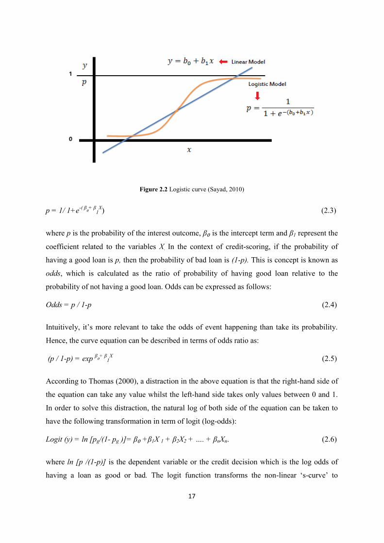
17

Figure 2.2 Logistic curve (Sayad, 2010)

p = 1/ 1+e-( β₀+ β

1X) (2.3)

where p is the probability of the interest outcome, β₀ is the intercept term and β1 represent the

coefficient related to the variables X. In the context of credit-scoring, if the probability of

having a good loan is p, then the probability of bad loan is (1-p). This is concept is known as

odds, which is calculated as the ratio of probability of having good loan relative to the

probability of not having a good loan. Odds can be expressed as follows:

Odds = p / 1-p (2.4)

Intuitively, it’s more relevant to take the odds of event happening than take its probability.

Hence, the curve equation can be described in terms of odds ratio as:

(p / 1-p) = exp β₀+ β

1X

(2.5)

According to Thomas (2000), a distraction in the above equation is that the right-hand side of

the equation can take any value whilst the left-hand side takes only values between 0 and 1.

In order to solve this distraction, the natural log of both side of the equation can be taken to

have the following transformation in term of logit (log-odds):

Logit (y) = ln [pg/(1- pg )]= β₀ +β1X 1 + β2X2 + …. + βnXn. (2.6)

where ln [p /(1-p)] is the dependent variable or the credit decision which is the log odds of

having a loan as good or bad. The logit function transforms the non-linear ‘s-curve’ to

18

approximately straight line and to change the range of the proportion from 0–1 to –∞ to +∞

(Bewick et al., 2005). The intercept and coefficients of the logit function are estimated using

the maximum likelihood function, in which it is an iterative process that is responsible in

finding the best values that raise log likelihood (Bewick et al., 2005; Kleinbaum & Klein,

2010). Once knowing the odds of the logit function, the probability can be known and hence

the outcome between 0 and 1 can be achieved.

P = odds / 1+odds (2.7)

Unlike LDA, LR does not require multivariate normal distribution of data. However, the LR

is exposed to a full linear relationship between the independent variable when related to the

logit of dependent variable (Lee & Chen, 2005). Moreover, if data are non-linear, the

Accuracy of LR decreases (Ong et al., 2005). Furthermore, according to West (2000),

Thomas (2000) and Akkoc (2012), LR and LDA are designed for problems where the

relationship between variables is linear; therefore, this might lead to deficiency in models’

predictive performance.

Despite the limitations, LR is an easy technique and is more suitable for credit-scoring than

LDA (Press & Wilson, 1978) and is recognised as the industry standard for building credit-

scoring models (Lessmann et al., 2015); this has been widely adopted in the literature

(Wiginton, 1980; Steenackers & Goovaerts, 1989; Hand & Henley, 1996; Desai & Crook,

1996; Baesens et al., 2003; Deasi et al., 2009; Crook et al., 2007).

2.3.3 DT

DT is another commonly used approach for classification purposes in credit-scoring

applications. It is also well-known as recursive partitioning method (Hand & Henley, 1997)

and classification and regression trees’ CART (Breiman et al,, 1984; Lee et al., 2006; Zekic-

Susac et al., 2004). DT are non-parametric classification techniques used to analyse

dependant variables as a function of independent variables (Arminger et al., 1997; Lee et al.,

2006). As shown in Figure 2.3, DT use graphical tools; the node is shown in the box with

lines to show the possible events and consequences, until reaching the best and optimal

outcome. The idea behind the DT in credit-scoring is to provide a classification between two

classes of credit ‘good’ and ‘bad’ loans. It begins with a root node that contain the two types

of class, with the node then being split into two subsets with possible events based on the

19

chosen variable or attribute, and so are the nodes, until the decision algorithm loops on all the

splits to find the optimal split and select the wining sub-tree which gives the best partitioning

of mostly ‘good’ and ‘bad credit based on its overall error rate and lowest misclassification

cost (Biermann et al., 1984; Thomas, 2000).

Total Loans = 10

Good loans = 5

Bad loans = 5

Creditworthy = 50%

Total Loans = 6

Good loans = 4

Bad loans = 2

Creditworthy = 66%

Total Loans = 4

Good loans = 1

Bad loans = 3

Creditworthy = 25%

Age > 35 Age <= 35

Total Loans = 4

Good loans = 4

Bad loans =0

Creditworthy = 100%

Total Loans = 2

Good loans = 0

Bad loans = 2

Creditworthy = 0%

Married Single

Figure 2.3 Example of DT for credit-scoring

A problem seen to arise in building DT is the goodness of split, which is what variable to

choose to grow the tree that could discriminate between classes (Mingers, 1989). In general,

the selection of the variable is based on the purity of the split, where several approaches are

available for splitting (Berzal et al., 2002), where the common one used is the information

entropy, which is based on the highest information gained from each attribute (Berzal et al.,

2002; Osei-Bryson, 2006). After finishing building the DT, some sections of the tree with less

predictive ability can be removed or pruned; this can reduce the complexity of the tree, hence

achieving better Accuracy by reducing overfitting (Mansour, 1997). Some pros of DTs are: 1)

Easy and interpretable; 2) Handles missing values; 3) They hold nominal and numeric

attributes; and 4) They don’t make assumptions about data distribution. Some cons include

the fact that DTs are: 1) sensitive to irrelevant attributes and noise; 2) DTs take a great deal of

effort in handling missing values (Rokach & Maimon, 2008); and 3) DT lacks robustness and

performance optimality (Lariviere & Van den poel, 2005).

Makowski (1985) was the first to introduce DTs in credit-scoring, and then it was

investigated in building credit-scoring models in various contexts, such as credit cards,

20

consumer loans, business failure and corporate loans (Srinivasan & Kim, 1987; McKee &

Greenstein, 2000). On the other hand, different forms of DT models were used as a

comparison with other techniques, such as LDA and LR: for example, in Lee et al. (2006),

Henley & Hand (1996) and Yeh & Lien (2009). DT was superior to LDA and LR, whilst it

was inferior in other works (West, 2000; Baesens et al., 2003; Zhou et al., 2009).

2.3.4 NB

NB classifiers are statistical classifiers that predict a particular class (good or bad) loan.

Bayesian classification is based on Bayesian theory and is a valuable and helpful measure

when the input feature space is high (Bishop, 2006). This is considered a very simple method

for making classification rules that are more accurate than those made from other methods;

therefore, very little attention and focus was assigned to the credit-scoring domain (Antonakis

& Sfakianakis, 2009). NB is calculated using the posterior probability of a class by

multiplying the prior probability of a class before seeing any data with the likelihood of the

data given its class: for example, in the credit-scoring context, the assumption can be made

that the training sample set D = { x₁, x₂,….,xn}, where each x is made up of n characteristics

or attributes { x11, x12,…., x1n} and assisted with a class label c either good or bad loan. The

task of the NB classifier is centred on analysing these training set instances and determining a

mapping function ƒ: (x11,….,x1n} -> (c), which can decide the label of an unknown example x

= (x1,….., xn):

P (ci| x1,….., xn) = P (x1,….., xn | ci)* P (ci)/ P(x1,….., xn) (2.8)

where P (c| x1,….., xn) is the posterior probability of class c after seeing data x. P (x1,….., xn |

ci) is the likelihood of the data x belonging class ci. P (ci) is the prior probability of class ci

before seeing any data and finally P(x1,….., xn) is the probability of data on class ci .Bayesian

classifiers choose the class that has the greatest posterior probability P(ci |x1… xn) as the class

label, according to minimum error probability criterion or maximum posterior probability

criterion. That is, if P (ci | x) = max P(ci | x), then assigning x to a particular class ci can be

determined. For the purpose of structure simplicity, the NB classifier (Bishop, 2006) strongly

assumes that the variables of data are independent and not correlated; however, this is

considered a weakness since dependences between variables can exist (Antonakis &

Sfakianakis, 2009). Some advantages of NB classifiers include that they are easy to explain

and understand; it is fast to train and classify; resistant to irrelevant attributes and outliers

21

(Kohavi, 1996; Oded & Rokash, 2005). Regardless, the advantages of NB include good

performance n many classification tasks but poor performance in others (Ratanamahatana &

Gunopulos, 2003). However, NB has been investigated in some credit-scoring studies and has

not shown valuable performance compared to other methods (e.g., Baesens et al., 2003; Yeh

& Lien, 2009; Antonakis & Sfakianakis, 2009).

2.3.5 MARS

It is a non-parametric and non-linear regression technique developed by Friedman (1991),

which models the complex relationships between the independent input variables and the

dependent target variable. Multivariate Adaptive Regression Splines (MARS) is built using

piece-wise linear regression by modelling a sequence of linear regressions on different

intervals or splines (Briand et al., 2004). Each spline should be specified by finding the

suitable independent variable to fit.

Figure.2.4 demonstrates how MARS fit data onto each linear regression spline. As can be

seen, each spline or interval is separated by what is referred to as a knot, which indicates the

end of an interval and the beginning of another one. This also indicates changing in the

behaviour of the dependent variable y or, in other words, knots are the place where the

behaviour of linear regression function change.

Figure 2.4 MARS example on linear regression intervals and knot locations (Briand et al., 2004)

In the figure, knots are labelled by x1 and x2, identifying three different linear relationships on

each interval or spline. In MARS, identifying and determining the knots’ locations is done by

a searching mechanism. MARS built a model in the form of:

22

y = c0 + ∑ ‍𝑘𝑖=1‍ ci *Bi(x) (2.9)

where c0 is a constant coefficient, Bi(x) is the basis functions and ci is a coefficient for the

basis functions. MARS use what is referred to as the basis function, taking numerous forms of

independent variables interactions. The common functions used are the hinge functions that

are used to find variables, which are selected as knots; hence, the function takes the following

form (Miguéis et al., 2013):

max (0, X – c) or, (2.10)

max (0, c –X) (2.11)

where c is constant, threshold or knot location, X is the independent variable. The goal behind

the basis functions is to transform the independent variable X in to a new variable (e.g., X*).

Based on equations 2.10 and 2.11 X* will take the value of X if X is greater than c and it will

take value of zero if the value of X is less than c (Briand et al., 2004). The knots’ locations c

is determined by forward/backward stepwise criteria, where many basis functions create

many knots, allowing interactions between different independent variables. Later, these knots

are pruned based on their contribution to the overall fit of the model (Lee et al., 2006;

Miguéis et al., 2013). An important advantage of MARS is that it can identify the importance

of each independent variable to the dependent variable when various possible independent

variables are measured (Lee et al., 2006). MARS refits the model after removing all terms

involving the variable to be assessed and accordingly calculates the reduction in model error,

with all variables categorised according to their influence on the performance of the model;

the optimal MARS model is based on the lowest generalised cross-validation (GCV) measure

(Briand et al., 2004; Miguéis et al., 2013) (for more insight of the MARS modelling, refer to

Friedman (1991) and Hastie et al. (2001)). Therefore, in the context of credit-scoring, this

feature of MARS is exploited in building credit-scoring model, as it is mostly utilised to

obtain a subset of the most significant variables based on their relative importance on the

model and use it as an inputs for the ordinary model (Lee et al., 2005; Lee et al., 2006; Chen

et al., 2009; Chuang & Lin, 2009). A strong advantage of MARS is that it is easy to

understand the model and it does not require a long training process (Lee et al., 2005).

23

2.3.6 NN

NN are machine-learning systems based on the concept of Artificial Intelligence (AI) inspired

by the design of the biological neuron (Haykin, 1999). NN models are modelled in such a

way to be able to mimic the human brain functions in terms of capturing complex

relationships between the inputs and outputs (Bhattacharyya and Maulik, 2013). In credit-

scoring context, NNs has been identified as an effective tool used in building credit-scoring

models as an alternative to the statistical techniques such as LDA and LR (Atiya, 2001;

Angelini, 2008). One of the most common architectures for NNs is the multi-layer perceptron

(MLP), which consists of one input layer, one or more hidden layers, and one output layer

(Jensen, 1992). According to Angelini (2008), one of the key issues needing to be addressed

in building NNs is their topology, structure and learning algorithm. The most commonly

utilised topology of NNs model in credit-scoring is the three-layer feed-forward back

propagation (FFBP). Figure 2.5 illustrates the architecture of common topology of NN based

on interconnected three layers FFBP.

Figure 2.5 The topology of back propagation (FFBP) NN (Al-Hnaity et al., 2015)

Consider the input of credit-scoring training set x = {x1, x2,…, xn}, the NN model works in

one direction, starting from feeding the data x to input layer (x includes the customer’s

attribute or characteristics). These inputs then are sent to a hidden layer through links or

synapsis, associated with random initial weight for every input. The hidden layer will process

what it has received from the input layer and accordingly will apply it to an activation

function. The results are served as a weighted input to the output layer, which will further

24

process weighted inputs and apply activation function, which will lead to a final decision. The

following steps the steps illustrate the training computations of the NN, all neurons in the

hidden layers are calculated as follows:

ni = ƒ H (‍∑ ‍𝑁𝑗=1‍ xj.wji), i = 1,2,…..,S (2.12)

where ni is the output of the hidden layer, ƒ H is the activation function (threshold) applied on

the value of each node in the hidden layer, activation function can take many forms the most

common one is the sigmoid function. Hence, the output of the hidden layer is passed with

other weights to the output layer, which is computed as follows:

yt = ƒ t (‍∑ ‍𝑆𝑖=1‍ ni.wit), t = 1,2,…..,L (2.13)

where yt is the output of the final decision after applying the activation function (threshold) on

the value of each node in the output layer. If the difference between final decision and the

actual target is significant, the back propagation learning algorithm will revert and update the

weights between hidden layer and output layer, and the weights between inputs and hidden

layer, with computation completed again until the difference between, with the NN computed

again until the final decision and the actual target is minimised. Building an NN model

involves training procedure for the variables in order to differentiate between that to get a

better decision and results. However, if the results are improper, the estimated values are

changed by the NN model until they become proper and acceptable (Abdou & Pointon,

2011).

The NN tend to establish the relationship between a customer’s probability of default and

their given characteristics, which then are filtered, and with the most important prediction

variables amongst them identified. The main advantages of NNs models is that it can handle

incomplete, missing or noisy data and requires no prior assumptions relating to the

distribution of the variables (Vellido et al., 1999). Moreover, it has the ability to recognise

complex patterns between input and output variables and accordingly predict the outcome of

new independent input data (Keramati & Youssefi, 2010). On the other hand, NNs are

criticised and lack explanatory capability, such that it cannot give an explanation or

justification as to how customers are chosen as either ‘good’ or ‘bad’, accepted or rejected.

Another shortcoming in NN is the selection of parameters as there is no official method to

select the appropriate parameters for the model, which might affect its prediction Accuracy

25

(Vellido et al., 1999; Lahsasna et al., 2010). Several studies have proven that NNs

outperformed statistical techniques (e.g., LDA, LR, NB and MARS) in prediction Accuracy

(West, 2000; Baesens et al., 2003; Desai et al., 1996; Malhorta & Malhorta, 2003; Lee &

Chen, 2005; Abdou et al., 2008).

2.3.7 SVM

SVM is another powerful machine-learning technique used in classification and credit-

scoring problems. It is being widely used in the area of credit-scoring and other fields for its

superior results (Huang et al., 2007; Lahsasna et al., 2010). SVMs first were proposed by

Cortes & Vapnik (1995), adopting the form of a linear classifier. SVMs take a set of two

classes of given inputs and predict them in order to determine which of the likely two classes

have the output. SVMs are used for binary classification in order to make a finest hyperplane

(Line) that categorize the input data in two classes (good and bad credit) (Li et al., 2006).

Figure 2.6 shows the foundation of SVM.

Figure 2.6 The basis of SVM (Li et al., 2006)

According to Figure 2.6, an input training vector should be assumed (x1,y1), (x2,y2),…, (xn,yn)

exists, where x ∈ Rd, which is a vector in d-dimensional feature space and yi ∈ {1,+1} is the

class label. Next step is to build a dividing hyperplane, which could be described like:

𝑤 ⋅ 𝑥 − 𝑏 = 0 (2.14)

Vector 𝑤 is orthogonal to diving hyperplane, and parameter 𝑏/𝑤 is equal to the distance from

the dividing hyperplane to the centre of coordinates. Since the goal is to find for the optimal

separation, finding bearing vectors and hyperplanes is needed. However, they can be

represented with these equations:

26

𝑤. 𝑥 − 𝑏 = 1 (2.15)

𝑤. 𝑥 − 𝑏 = −1 (2.16)

where 1 and –1 are coefficients dependent on the normalising. If the data is linearly separable,

than the only task left is to find‍𝑤 and‍𝑏‍. In such a case that data are non-linear, other types

would be proposed in order to improve the Accuracy of the original model. The main

difference of the new model, compared to the initial model, is the function used to map the

data into a higher dimensional space. New functions were proposed, namely linear,

polynomial, radial basis function (RBF) and sigmoid.

SVMs map non-linear data of two classes to a high-dimensional feature space, with a linear

model then used to implement the non-linear classes. The linear model in the new space will

denote the non-linear decision margin in the original space. Subsequently, SVMs will

construct an optimal line (hyperplane) that could perfectly separate the two classes in the

space. The advantages of the SVM lie in its capability in model non-linear data, which

delivers high prediction Accuracy compared with other techniques. The disadvantages of

SVM include that it is difficult to understand, which might lead to hesitation in its use

(Martens et al., 2007); many studies, on the other hand, have adopted SVMs in building

credit-scoring models (Zhou et al., 2009; Bellotti & Crook et al., 2009; Li et al., 2006; Huang

et al., 2007; Chen & Li, 2009).

2.3.8 RF

RF is considered an advanced technique of DTs, as proposed by Biermann (2001), which

consists of a bunch of DTs that are created by generating n subsets from the main dataset,

with each subset a DT created based on randomly selected variables, which is why it is

referred to as RF, since a very large number of trees are generated. After all DTs are

generated and trained, the final decision class is based on voting procedure, where the most

popular class determined by each tree is selected as a final class for the RF. Figure 2.7

illustrates the RF architecture.

27

Figure 2.7 RF architecture (Verikas et al, 2011)

Regardless of the simplicity of DTs, it has disadvantages that have been addressed by

researchers focused on optimising the DT technique, where such efforts lead to the

developing of RF (Biermann, 2001; Lariviere & Van den poel, 2005). The main two

parameters to be set when building an RF are the number of tress and the number of variables

or features needing to grow each DT (Brown & Mues, 2012). According to Breiman (2001),

the process of building an RF starts by:

Creating random bootstraps from the training set with replacement.

On each bootstrap, building several DTs by selecting random variables from each

subset.

The starting node of each DT is selected with the high information gain.

The tree will grow up until no more nodes can give more information about the class,

there is no pruning.

A voting procedure then will take place between the several DTs leading to the final

class decision of the RF.

According to Miner et al. (2009), RFs have many remarkable advantages: 1) it gives

relatively high Accuracy amongst other classification techniques; 2) It is robust in handling

missing data; 3) It can handle any size data and variables; 4) It can detect the variables with

high influence on the classification results; and 5) It is fast to run and easy to use. A limitation

in RF is that it cannot handle very large numbers of irrelevant attributes (Grosan & Abraham,

2011).

28

RF has been afforded much attention since its introduction and has become a very popular

technique in classification and other measures, and has been applied in many fields, such as

bioinformatics, image processing, chemistry and credit card fraud detection (Verikas et al.,

2011). However, in the credit-scoring context, RF has not been investigated widely, yet it

has shown good classification results (Brown & Mues, 2012; Wang et al., 2012; Lessmann et

al., 2015).

2.4 Credit-Scoring Modelling Approaches

In the previous section, the state-of-the art quantitative approaches from statistical to

machine-learning techniques that are mostly used in developing credit-scoring models were

overviewed. The reliability of the credit-scoring model is measured in terms of its accuracy.

In this section, the approaches and the ways of utilising these techniques in building credit-

scoring models is covered.

2.4.1 Individual Classifiers

In order to develop a credit-scoring model, a classifier should be selected to fulfil this task.

However, many techniques have been proposed during the last decades, the aim of which was

to build a good performing credit-scoring model that serves the purpose for which it was

built. The selection of a classifier that could do its best is based on the nature of the problem,

dataset size, variables used and the market environment for which it is developed (Hand &

Henley, 1997). The early credit-scoring models started using statistical techniques, such as

LDA and LG as common methods; however, they have shown various shortcomings that lead

to being replaced by other new machine-learning techniques that produce more rigorous

models, such as NN, SVM and DTs. Several studies have investigated the use of individual

classifiers in constructing credit-scoring models for example (Desai et al., 1997; Malhotra &

Malhotra, 2003; Zekic-Susac et al., 2004; Lee et al., 2006).

According to Khashei et al. (2009), using individual classifiers in building credit-scoring

models might give accurate and precise models, but there are some negatives for both of

them; they are considered to use classical logic process in their modelling, they cannot

efficiently model complexities and uncertainties. For this reason, researchers have directed

their efforts towards finding different ways and approaches to utilising these techniques to get

more reliable, credible and accurate results.

29

2.4.2 Hybrid Techniques

Hybridisation or hybrid models are a new method in building credit-scoring model and have

been widely adopted in the literature. The concept of hybrid modelling is to combine one or

more classifiers together in order to give higher prediction Accuracy (Khashei et al., 2013).

The main purpose of hybrid models is to condense the risk of choosing an improper model

when solving a problem. However, the basic idea of combining several classifiers is to get

benefits of the unique features of each classifier in order to capture different patterns of the

characteristics of the dataset, which will lead to an efficient credit-scoring model with highly

improved results. Every individual classifier has strong and weak points; however, the notion

of hybrid techniques is to overcome weaknesses and exploit strengths of each classifier by

integrating techniques together (Khashei et al., 2012; Sadatrasoul et al., 2013).

The idea behind a hybrid model is to combine two models or techniques in sequential process

where one model is trained to serve as an input for the other model to perform the

classification task. According to Li & Zhong (2012), there is no clear solution on how to

classify hybrid models; hence, in their study, Tsai & Chen (2010) divided the hybrid models

structure by combing classification techniques and clustering techniques through all possible

ways.

The main aim of the first classifier is either to be trained or pre-processed. Its output then is

fused to train the next classifier or clustering technique. The simplest way of building a

hybrid model is through three steps: 1) Feature selection as pre-processing step; 2) Model

parameters selection; and 3) Classification (Li & Zhong, 2012). The pre-processing step

comprises feature selection that selects the most significant features as a new feature subset to

the new classifier. Moreover, data pre-processing can also comprise feature extraction,

clustering and data-filtering (for more details refer to Verikas et al. (2010) and Garcia et al.

(2012)). More about the data pre-processing step is discussed in detail in the next chapter.

30

2.4.3 Ensemble Techniques

Alongside the hybrid techniques, another method used by researchers is the ensemble

learning method or multiple classifier system, which have become the most recent methods in

credit-scoring evaluation (Lin & Zhong, 2012). These techniques have widely attracted the

attention of researchers in the field of credit-scoring over the last decade, with many having

combined multiple classifier systems in different ways in order to achieve high prediction

performance classifiers (Tsai, 2014; Nanni & Lumini, 2009). The ensemble method is an

approach that applies multi-classifiers rather than single classifiers in order to achieve higher

Accuracy results. Moreover, the difference between ensemble and hybrid methods is that the

ensemble output of the multiple classifiers is pooled to give a decision whilst, in hybrid

methods, only one classifier gives the final output, whereas the other classifier results are

processed as an input to the final classifier (Verikas et al., 2010). A central key issue in

building an ensemble classifier is to make each single classifier different from the other

classifiers as possible; in other words, to be as diverse as possible (Nanni & Lumini, 2009).

The ensemble method in building the credit-scoring models is valued due to its ability to

outperform the best single classifier’s performance (Kittler et al., 1998). The basic idea of

ensemble classifiers is to generate multi-classifiers and accordingly combine their

information in order to reduce the variance of single classifier estimation errors and increase

the overall classification outcomes. In addition, the ensemble method seeks to construct a set

of assumptions and combine them to establish the desired results—not as a single classifier,

which only learns one assumption from the dataset (Wang & Ma, 2012). Practically, building

an ensemble of classifiers involves three main steps: 1) System topology; 2) Classifier

generation; and 3) Classifier fusion or combination (Zhang & Duin, 2010; Wozniak et al.,

2014). Firstly, the topology of building the ensemble model can take two structures: the

parallel and serial structures. The parallel structure is the most commonly used structure in

building ensemble models in the literature; this is based on training the individual classifiers

on the same input data. The serial ensemble structure involves the individual classifiers being

applied in sequence order, so that the output of the first classifier is used as new data to the

next classifier, classifier after classifier, until the classifier is confident about its output

(Wozniak et al., 2014). The parallel ensemble structure is adopted in this thesis.

The second step includes the generation of the classifier; practically, there are two common

ways of generating an ensemble of classifiers. The first is to build the classifiers using the

31

same type of learning algorithm that could be with different parameters; this way is

homogenous classifier. The other way is to build the ensemble using different types of

learning algorithm (Zhang & Duin, 2011). Alternatively, different classification algorithms

can be applied to make the ensemble, with the idea being that the different classifiers have

different views on the same data and can complement one another (Lessmann et al., 2015;

Zhang & Duin, 2011). However, these generated classifiers, in either way, are trained on

different data or different features of the training dataset. That is, different classifiers are

trained on diverse parts of data, meaning each trained classifier will generalise in different

ways (Tsai & Wu, 2008; Zhang & Duin, 2011). The most popular approaches for modifying

training data are cross-validation, bagging and boosting (West et al., 2005).

After all classifiers give their decisions, they are pooled in order to combine and fuse them by

some rule or method, here comes the third step. Usually, when combining ensemble outputs

two approaches are utilised namely classifier fusion and classifier selection (Canuto et al.,

2007; Kheradpisheh et al., 2013). The classifier fusion considers combining all classifiers

predictions that are trained to the whole problem, with a combination rule accordingly applied

to combine them. Some common ways of combining classifiers are majority voting (MajVot),

weighted average (WAVG), weighted voting (WVOT), mean (AVG), maximum rule (MAX),

minimum rule (MIN) and product rule (PROD) (Canuto et al., 2007; Zhang & Duin, 2011;

Tsai, 2014); besides, these methods also are considered as fixed or static combiners (Zhang &

Duin, 2011; Xiao et al., 2012). These fusion methods could be the best option for combining

multiple classifiers owing to their simplicity and good performance (Zhang & Duin, 2011).

On the other hand, classifiers ensemble selection is based on selecting the classifiers that do

well on each input data; classifier selection that best fit each input data is made during

running phase. A popular method used in this matter is the dynamic classifier selection based

on local Accuracy (DCS-LA) where the output of each data is based on its local Accuracy

(Woods et al., 1997; Canuto et al., 2007; Zhang and Duin, 2011; Xiao et al., 2012) (For

further reading about classifier selection combination methods, please refer to Canuto et al.

(2007) and Zhang & Duin (2011).

32

2.5 Model Performance and Significance Measures

After finishing from training the model, it must be validated for its efficiency by applying it

to an unseen sample; however, there exist many performance indicators that can designate the

efficiency of the developed model. According to Hand (1997), a range of performance

measures indicators are available. The most common performance measures adopted in

credit-scoring is the Accuracy rate of the model, which shows how many instances where

classified correctly. Another measure is the error rate of the model which is 1 – Accuracy;

this indicates how many instances are misclassified by the model. However, as the problem in

credit-scoring is a binary class problem the decisions made by the model can take the form of

a 2×2 confusion matrix as shown in Table 2.1.

Predicted

Actual Good loans Bad loans Accuracy

Good applicant TP FN (Type II error) Accuracygood

Bad applicant FP (Type I error) TN Accuracybad

PPV NPV Accuracytotal

Table 2.1 Confusion Matrix for Credit-scoring

It is clear from the above table that loans are in two groups good and bad loan applicant: if the

model correctly detected the good loans and the bad loans then it is a TP (true positive) and

TN (true negative), respectively, otherwise it is an FN (Type I error) and an FP (Type II

error), respectively. The Accuracy good and Accuracy bad indicates the model’s accuracy in

identifying good and bad loans, whilst the Accuracy total shows the overall Accuracy of the

model and how well it performs. Besides the predicted positive value (PPV) and negative

predicted value (NPV), the percentages of how many loans were predicted as good and bad

loans by the model correspondingly. In other words, it indicates how many applicants are

given a loan. Another common measure also used in the area of credit-scoring is the receiving

operating characteristic curve (ROC), which is a measure indicating the classification

performance of a model through a range of several thresholds, unlike the Accuracy, which the

performance of the model is based on pre-determined single threshold. Another measure,

known as the area under curve (AUC), is used for comparison across several classifiers. Other

uncommon measures are H-measure, Brier score, and Gini coefficient, which also are

33

addressed in credit-scoring (Lessmann et al., 2013). The purpose of investigating different

performance measures is centred on assessing the model from different aspects (Lessmann et

al., 2013).

Another important phase of investigating the efficiency of a credit-scoring model is that it is

robust, and its performance is not related to any factors associated during the development

process of building the model (Garcia et al., 2015). However, in order to achieve this, some

kind of hypothesis-testing should be carried out so as to assure that the model performance is

not a matter of luck. Many tests’ parametrical and non-parametrical significant statistical tests

can be utilised to validate the results of the model, such as in the case of the t-test, Friedman

rank test and Bonferroni-Dunn test. A greater insight into performance indicator measures

and statistical significance tests are discussed in the next chapter.

2.6 Credit-scoring Studies

The area of credit-scoring has been a widely investigated topic in the literature for the last

five decades. Significant studies have been adopted on assessing the performance of

individual credit customers and corporate credit customers, which also are known as

bankruptcy prediction. This thesis will be strict on the area of dealing with individual credit

customers and, specifically, on the quantitative approaches used in developing credit-scoring

models for these customers. Many approaches have been utilised, from statistical to machine-

learning techniques. Such methods were used in different ways, from implementing single

classifiers, hybrid models and ensemble models and the main aim were to achieve a reliable

and efficient model that can serve the purpose it was developed for. Since adopting the simple

statistical approaches such as LDA and LR to score and assess customers’ creditworthiness,

these approaches have been widely used till the emerging of machine-learning techniques that

were believed to fill the shortcomings of the statistical techniques.

In practice, real historical datasets are used in order to develop credit-scoring models; these

datasets might differ in size, nature, and the information or characteristics it holds, whilst

individual classifiers might not be able to capture different relationships of these datasets

characteristics. As a result, researchers have employed hybrid modelling techniques that can

exploit the strength and compensate weaknesses of different classifiers in learning the

relationships between data. From hybrid-modelling, researchers have inspired the ensemble

modelling, which gives classifiers the opportunity express their ability to learn data on

34

different parts of data and feature space. Almost all studies reported that hybrid and ensemble

modelling is superior to individual classifiers; for this reason, this thesis will focus on the

studies that applied hybrid and ensemble techniques in the field of customer credit-scoring.

Prior to starting the representing and summarising of related studies, the mechanism of how

the related work was collected is explained.

2.6.1 Literature Review Collection Process

The area of credit-scoring is an important topic in finance and data classification, and it has

been expected to have received much focus through the completion of a large number of

studies related to the development of credit-scoring models. Firstly, the searching process for

the relevant work started with the typing the keywords ‘credit-scoring’, ‘credit customer

classification’, ‘hybrid models’ and ‘ensemble models’ in the relevant fields, supported by

five most widely known and used academic science databases, namely ‘Google Scholar’,

‘Science Direct’, ‘IEEE Xplore’ and ‘Springer’. The search provided results centred on topics

related to credit-scoring, credit risk and bankruptcy prediction. The intended search of papers

ranged from 2002 up to 2015, and the results included huge resources comprising many

journal papers, articles, books and conference papers.

Secondly, only journals papers were included in the further search as these were considered

better related to the new developments in the credit-scoring field than books and were

believed to contain more in-depth explanations about methods used than conference papers.

In the filtering stage, it seems that papers containing credit risk and bankruptcy predictions

were related or were seen to have the same concept of credit-scoring in terms of the datasets

used in validating the developed model or in the motivation of proposing methods that

increase model performance. All the papers that aimed at using individual classifiers only to

develop models were excluded as the aim is centred on collecting papers that used hybrid and

ensemble models; however, these studies included individual classifiers as a benchmark.

Thirdly, all related studies are selected and organised in sequential order from 2002 till 2015,

with all the findings of studies comprehensively summarised and discussed based the

experimental design of studies, the features of the datasets used, the classification techniques

used, the ways of how data is pre-processed, the modelling approaches, performance indicator

measures and hypothesis testing employed.

35

2.6.2 Literature Discussion and Analysis

A collection of 37 papers was selected from various rigorous scientific journals with the focus

on hybrid, ensemble, data-pre-processing studies and studies that focused on improving or

proposing new approaches in credit-scoring. Table 2.2 summarises all the collected related

studies that contain valuable information and findings that could lead to reliable conclusions.

No.

Study

No. D

ata

sets

Data

splittin

g

Data

pre-

processin

g

Data

pre-

processin

g

Tech

niq

ue

No. C

lassifier

s

Base

Cla

ssifiers

Hyb

rid

ap

proach

Ensemble approach

Perfo

rm

an

ce

measu

res

Sig

nifica

nt te

st

Classifiers Combination

rule

1 Lee et al.

(2002) 1

Hold-

out

Feature

selection LDA 3

LDA, LR,

NN Yes - - Acc, Type & II errors -

2 Hseih (2005) 2 K-fold Clustering SOM, K-

means 1 NN Yes - - Acc, Type & II errors -

3 Lee and Chen

(2005) 1

Hold-

out

Feature

selection MARS 4

LDA, LR,

NN,

MARS

Yes - - Acc, Type & II errors,

EMC4 -

4 West et al.

(2005) 3

Hold-

out - 4 NN - Homogenous MajVot, WAVG Acc Yes

5 Huang et al.

(2006) 2

Hold-

out

Feature

selection GP 6

GP, NN,

LR,

DT(CART

, C4.5), k-

NN

Yes - - Acc -

6 Huang et al.

(2007) 2 K-fold

Feature

selection

Grid

search, F-

score, GA

4 SVM, NN,

DT Yes - - Acc -

7 Tsai and Wu

(2008) 3

Hold-

out - - 1

NN

ensemble - Homogenous MajVot Acc, Type & II errors Yes

8 Yu et al.

(2008) 3

Hold-

out - - 7

LR, SVM.

NN

ensemble

-

Homogenous/S

elective

ensemble

MajVot,

Reliability-based1 Acc, Type & II errors -

9

Nanni and

Lumini

(2009)

3 Hold-

out - - 12

Ensemble

of LMNC,

NN, k-NN,

SVM

- Homogenous Sum rule Acc, Type & II errors,

AUC Yes

10 Sustersic et

al. (2009) 1 K-fold

Feature

selection PCA, GA 2 LR, NN Yes - - Acc, Type & II errors -

36

11 Bellotti and

Crook (2009) 1

Hold-

out

Feature

selection SVM 4

LR, LDA,

k-NN,

SVM

- - - AUC -

12 Chen et al.

(2009) 1

Hold-

out

Feature

selection

MARS,

DT(CART) 5

SVM, DT

(CART),

MARS

Yes - - Acc, Type & II errors -

13 Chunag et al.

(2009) 1

Hold-

out

Feature

selection MARS 5

LDA, LR,

DT(CART

), NN,

CBR

Yes - - Acc, Type & II errors -

14 Yu et al.

(2009) 3

Hold-

out - - 10

LDA, LR,

NN, SVM,

Ensemble

of NN and

SVM

- Heterogeneous Fuzzy GDM2 Acc, Type I & II errors,

AUC Yes

15 Tsai (2009) 5 K-fold Feature

selection

t-test,

Stepwise,

F-score,

CM, PCA

6 NN - - - Acc, Type I & II error

16 Chen and Li

(2010) 2

Hold-

out

Feature

selection

LDA, F-

score, DT,

Rough sets

1 SVM - - - Acc Yes

17 Zhou et al.

(2010) 2

Hold-

out - - 25

LDA,

QDA19,

LR, NN,

DT, NB,

PR20

-

Homogenous/

Selective

Ensemble

MajVot,

Reliability-based,

Weights based on

tough samples

Acc, Sn, SP, AUC

18 Hseih and

Hung (2010) 1 K-fold - - 4

SVM, NN,

NB - Heterogeneous

Confidence

WAVG Acc -

19 Zhang et al.

(2010) 2 K-fold

Feature

selection Rough sets 11 DT Yes Homogenous MajVot Acc -

20 Tsai and

Chen (2010) 1

Hold-

out

Feature

selection/

Clustering

K-means,

EM 12

LR, DR,

NB, NN Yes - - Acc -

21 Yu et al.

(2010) 1

Hold-

out - - 8 SVM - Homogenous

MajVot, WAVG,

ALNN3

Acc, Type I & II errors,

AUC Yes

22

Chuang and

Hunag.

(2011)

2 Hold-

out

Feature

selection Rough sets 5

LDA, LR,

NN, CBR Yes - -


AUC -

23 Wang et al.

(2011) 3

Hold-

out - - 13

LR, DT,

SVM, NN -

Homogenous/

Heterogenous

MajVot, WAVG,

Stacking Acc, Type I & II errors -

37

24 Finlay (2011) 2 K-fold Feature

selection Stepwise 18

LDA, LR,

DT

(CART),

k-NN, NN,

Ensemble

of all

above

- Homogenous MajVot, WAVG,

Mean Classification Error Rate Yes

25 Akkoc

(2012) 1 K-fold

Feature

selection LDA, LR 4 NN Yes - -


AUC, EMC -

26 Wang and

Ma (2012) 1 K-fold - - 13

DT,

Ensembles

of DT

Yes Homogenous MajVot Acc, Type I & II errors Yes

27 Wang et al.

(2012) 2 K-fold - - 11

LR, NN,

DT, SVM,

Ensemble

of SVM

Yes Homogenous MajVot Acc, Type I & II errors -

28 Marques et

al. (2012a) 6 K-fold - - 17

Ensembles

of k-NN,

NB, LR,

NNs,

SVM, DT

(C4.5)

- Homogenous MajVot Type I & II errors, AUC Yes

29 Marques et

al. (2012b) 6 K-fold - - 35

of k-NN,

NB, LR,

SVM,

DT(C4.5),

Ensembles

of DT

(C4.5)

- Homogenous MajVot Acc, Type I & II errors Yes

30 Brown and

Mues (2012) 5

Hold-

out - - 10

LR, NN,

DT (C4.5),

LDA,

QDA, RF,

k-NN,

SVM,

GB21

- Homogenous MajVot AUC Yes

31 Tsai and

Cheng (2012) 4 K-fold

Data-

filtering K-means 4

NN, DT,

SVM, LR - - - Acc, Type I & II error -

32 Garcia et al.

(2012) 8 K-fold

Data-

filtering

20 filtering

algorithms 20 k-NN Yes - - Acc Yes

33 Xiao et al.

(2012) 2

Hold-

out - - 8

DT

(CART) -

Selective

Ensemble

MajVot,

WMajVot Acc, Sn, Sp, AUC -

34 Tsai (2014) 5 K-fold Clustering SOM, K-

means 21

LR, NN,

DT

(CART)

Yes Homogenous/

Heterogenous

MajVot,

Weighted Vote Acc, Type I & II errors Yes

35

Abellan and

Mantas

(2014)

3 Hold-

out - - 5

LMNC,

DT (C4.5,

CDT22)

- Homogenous MajVot AUC Yes

38

Ensembles

of all

above

36 Harris (2014) 2 Hold-

out Clustering K-means 8 SVM, LR - - -

Acc, AUC, BAC5, Sn,

Sp Yes

37 Lessmann et

al. (2015) 8 K-fold - - 41

Refer to

paper -

Homogenous/

Heterogenous/

Selective

Ensemble

MajVot, WAVG,

Stacking

Acc, AUC, Brier Score,

KS6, PG7, H-measure Yes

Total 102 19 14/2/4 - 369 - 16 14/5/4 - 37 16

Average 2.7 - - - 9.9 - - - - - -

1Acc: Accuracy, 2Sn and Sp: Sensitivity and Specificity, 3 Reliability-based: minimum, maximum, mean, median, and product rules, 4GDM: group decision

making. 5 ALNN: adaptive linear neural network. 6 EMC: expected misclassification cost. 7 BAC: balanced Accuracy.8 KS: Kolmogorov-Smirnov. 9 PG: Partial

Gini index. 10SOM: 10Self Organizing Map. 11GP: Genetic Programming. 12GA: Genetic Algorithm.13Levenberg–Marquardt neural net.14CBR: Case Based

Reasoning.15EM: Expected Minimization algorithm.16PCA: Principal Component Analysis. 17CM: Correlation Matrix. 18FA: Factor Analysis.19QDA: Quadratic

Discriminate Analyses. 20PR: Probit Regression.21GB: Gradient Boosting. 22CDT: Credal Decision Trees.

Table 2.2 Related studies comparison

Table 2.2 summarises all the related studies, taking into consideration various essential

factors that make up the development process of any credit-scoring model. The number of

datasets used to validate the model with, data-splitting techniques that are responsible for

evaluating and assessing the model, the data pre-processing that deals with analysing the data

in terms of noise and outliers, and preparing clean data to be trained in order to achieve better

performance. Moreover, the number of classifiers used in each study is important as it reflects

the extent to which classifiers are used to compete with one another. Moreover, the

experimental design approaches, whether hybrid or ensemble approaches, are considered, as

well as the performance indication measures used in each study and the significant tests

associated to proving the reliability and robustness of the developed models.

Overall, findings that will give us information about what has been done or tackled so far in

the field of credit-scoring are summarised, including the procedure of building or designing

credit-scoring models, and the extent to which these could help or lead to addressing areas

that are not fully investigated or afforded attention in the field of credit-scoring. As a result,

we are guided in reaching a systematic comprehensive model that comprises new approaches

on different aspects of the model. It is worth noting that this thesis is focused on proposing

new approaches in the field of credit-scoring rather than comparing classification results with

the related studies.

Various findings and conclusions can be derived from Table 2.2. The first finding is that the

majority of the studies (30 out of 37) used between 1 and 3 datasets to evaluate their models.

39

A total of 2 studies used 8 datasets; however, on average, the number of datasets used in all

related studies equated to approximately 3, which are relatively small. Going in-depth into the

studies, the vast majority of them shared same common datasets, namely German and

Australian credit datasets (is discussed in more details in the next chapter), and according to

Lessmann et al. (2013), relying on these datasets for developing new models could lead to

bias. Moreover, these datasets might not reflect datasets used in industry as different datasets

could have different characteristics (Finlay, 2011). However, some studies used one private

dataset provided by banks and companies to validate their studies and other studies used

combined benchmarked and private datasets to extra validate their models. One main reason

for relying on German and Australian credit datasets is that they are publicly available for

researchers, with collecting industry datasets not an easy task due to confidential policies by

some financial institutions.

The second finding is related to splitting or partitioning the data used to train the model, with

the data assessing the model. As can be established, 21 studies used the hold-out splitting

technique and 17 studies used the k-fold Cross-validation (CV) splitting technique. Basically,

hold-out is cutting the dataset randomly into two parts: one part builds the model and the

other part assesses the model. The k-fold CV technique involves dividing the datasets into K

subsets (or folds) of equal size (K = 1, 2…, K), although K cannot exceed the size of the

dataset. Therefore, the model training is based K-1 folds, and the remaining K folds are saved

for model evaluation or testing. The process continues until all K folds are used for

evaluation. All the tested K fold predictions are used to estimate the model Accuracy (by

taking the average). Despite the attention towards these particular splitting techniques, there

are other ways of splitting the data, such as repeated hold-out, leave-one-out and k1xk2- fold

CV (Alpaydin, 2010; Garcia et al., 2015). According to Garcia (2015), the choice of each

splitting techniques to be employed depends on researcher preference. However, issues

should be considered prior to choosing a splitting technique, such as the stratification of data

samples based on their class and the size of the dataset(s) available.

Another important step in model-building is the pre-processing of data that is used to build up

the model. Principally, each dataset is made up of samples, where each sample consists of a

number of characteristics, attributes or features that vary in size depending on the nature of

the data. However, amongst these samples and features, there could exist outliers, noisy,

redundant or irrelevant features that may affect the performance of the model. The superiority

40

of the data is important in order to achieve better model performance, which is highly

dependent of the data efficiency in terms of number of data samples, the relevance of its

attributes or features and the presence of outliers in the dataset (Garcia et al., 2012).

Consequently, the cleaning or filtering of the unnecessary and redundant information can

consume time and costs, but also increase model performance (Tsai, 2009). Also another way

of pre-processing data, according to Tsai & Chen (2010), is clustering, which is another

method in data pre-processing used in building hybrid models; here, data are grouped or

clustered according to their similarities and dissimilarities. According to Saddatrasoul et al.

(2013), the clustering technique is done in order to identify and filter the outliers of the data,

and then the remaining ones that are not filtered are used to train the classifier in order to

improve the classification result. As can be seen from Table 15, feature selection was used as

a pre-processing step where only a subset of significant and relevant features was used to

train the model. Notably, only 2 and 4 studies embraced data-filtering and clustering,

respectively, for data pre-processing. In total, 21 studies applied the processing step for their

data, which is almost half of the studies; this reflects the importance of this step for enhancing

the model performance. All the studies reported achieving better model predictions than

without cleaning data from outliers and noisy information. Many methods are available for

feature selection, data-filtering and clustering, such as MARS, Relative neighbourhood graph

editing (RNG) and k-means (Lee and Chen, 2005; Garcia et al., 2012; Tsai, 2014). In general,

data on pre-processing has increased in importance and has become a fundamental step in

credit-scoring models development (Garcia et al., 2012).

Another major stage in model development is the development of the classifiers and how

these classifiers are used for comparison in each study. Well, as can be noticed from the table,

the number of classifiers developed and used in the related studies varied from small to large

(e.g., from 1 to 41 classifiers), providing an average of 9.9 classifiers. The reason behind the

varying numbers of classifiers in each study is that: 1) each study try in proposing new

methods and compare it with other methods within the same study (e.g., West et al., 2005;

Tsai & Wu, 2008; Marques et al., 2012a) or to 2) compare new developed methods with other

methods from other studies (Yu et al., 2008; Zhang et al., 2010; Wang et al., 2012; Abellan &

Mantas. 2014). In general, the number of classifiers used in a study depends on the developed

model and how many classifiers or methods are to be compared in order to prove its

validation and superiority. It is worth mentioning that Hand (2006) made some remarks on

studies, comparing their results with other study results, where the comparison could be fair

41

enough, as the author making the comparison might be more skilled in the method using and

the level to which he can tune it to achieve better results. In other words, there is no universal

superiority of a model on another, and reaching fair comparison factors, such as datasets used,

data-splitting techniques and performance measures employed, should be taken into

consideration in order to prove relative superiority.

In reference to the previous discussion, researchers tend to build classifiers that perform and

generalise the data well, whether by proposing novel ideas or creating different modelling

structures. One of the approaches used to enhance the model classification results is the

hybrid modelling, which is proven to be a superior approach in achieving high performance

when applied to credit-scoring problems. As discussed earlier, in Section 2.3.2, the

experimental design of this is achieved by integrating or uniting different methods or

classifiers together in order to exploit their strengths and overcome the weaknesses of each

method. As is clear from Table 2.2, 16 studies adopted hybrid modelling to achieve high

prediction performance. It can be noticed that all the hybrid modelling studies adopted feature

selection, clustering and data-filtering as a first stage in the hybrid model, where the

significant features or representative data to be used as training input for the classifier in the

second stage. Majority of the studies focused on applying feature selection, whilst only 4 and

2 studies focused on clustering and data-filtering, respectively.

Clustering is a technique used when data labels are not provided in which the group is data

based on their similarities, although credit-scoring datasets are labelled clustering techniques

and are applied in credit-scoring studies (e.g., Hseih, 2005; Tsai & Chen, 2010; Tsai, 2014).

Regarding feature selection and data-filtering, both are used to select the most appropriate

features and data to train the model.

Another experimental approach of modelling, as proposed to achieve better model

performance, is the ensemble approach. Unlike hybrid methods, ensemble learning creates

several classifiers with different types or parameter, such as several NN classifiers with

different structures, and accordingly train different samples of the dataset for several times,

with the right classifiers chosen as ensemble members. The results of the members are

pooled, with the ensemble strategies employed to get the final results (Lin & Zhong, 2012). In

creating the ensemble model, two points should be made in consideration of the selection of

the single classifiers. First, the classifiers should be successfully applied in credit-scoring

42

analysis. Secondly, the design of the classifiers should be based on different theoretical

concepts (Hseih & Hung, 2010). The important aspect of ensemble models is to be diverse

and accurate (Wang et al., 2011).

Table 2.2 shows that there are 19 studies that followed the ensemble modelling in their work.

This reflects the importance of the ensemble modelling approach in building a credit-scoring

model. Exploring the studies in-depth, all of them have followed the parallel structure, with

most of them adopting the bagging method so as to achieve diversity for the data that needs to

be trained in the model. After having the data ready, models have to be developed so as to

train the subsets of different data. Models can be developed in two ways: 1) building

homogenous classifiers where classifiers are all of the same type; or 2) building

heterogeneous classifiers where different types of classifiers are used to train the data. After

training, all or some of the model predictions are combined into a single classifier so as to

give a final answer or decision on the data. A total of 16 studies used homogenous ensemble

in their models (e.g., West et al., 2015; Tsai & Wu, 2008), whilst 5 studies used

heterogeneous ensemble (e.g., Yu et al., 2009; Hsieh & Hung, 2010; Tsai, 2014). Some

studies did not combine the classifiers’ predictions but rather chose the most appropriate and

representative ensembles for combining their predictions (Yu et al., 2008; Zhou et al., 2010;

Finlay, 2011; Lessmann et al., 2015).

Xiao et al. (2012) used dynamic classifiers ensemble using local Accuracy (DCE-LA) where

best ensembles are selected based on their ability to classify a certain data sample. DCE-LA

is done by computing the local Accuracy of a classifier with respect to output class of the data

sample in a region of competence, and classifiers with a high level of competence in

classifying the data point is selected for combination (Cruz et al., 2014). Another vital step is

classifiers combination and regarding the combination rules that are used to fuse all the

predictions of classifiers, majority vote (MajVot) is the most popular due to its simplicity;

weighted average (Wavg) was also used but with less frequency. Reliability-based methods

were only applied in 3 studies and stacking, which is considered a trainable combiner, was

employed in 2 studies.

Another major step is the evaluation of the model performance, which assesses how well it

will do in consideration to new data. With regards to performance measurements, measures

that can be derived from the confusion matrix average Accuracy (Acc) were used in almost

43

all studies, with Type I and Type II error appearing in 22 studies, and the sensitivity and

specificity appearing in 4 studies. The AUC was used in 12 studies. Lessmann et al. (2015)

investigated the use of new performance measures for credit-scoring, namely the inclusion of

Brier Score, KS, PG and the H-measure. Moreover, a new measure was used by Harris

(2014), which is the balanced Accuracy measure (BAC). From a practical perspective, each

of these methods expresses different views on model performance, meaning the important

issue is to use the most appropriate performance measures that fit the model concerns (Garcia

et al., 2015; Lessmann et al., 2015).

Finally, after assessing the model performance the model developers have to check whether

the model results are robust and reliable and it is not a pure coincidence. According to Garcia

et al. (2015) the statistical tests for model results is an important stage in the models

development process. However, as can be noticed, less than half of the studies employed

statistical significant tests on their proposed methods to determine whether the performance

of their proposed models was statistically significant than other compared methods. There are

several statistical tests of significance available for comparing and validating performance

results of different models, such as the parametric test (e.g., t-test) and non-parametric tests

(e.g., Friedman rank test, Bonferroni- Dunn test). Nonetheless, choosing the best test for

application depends on different aspects, such as the number of datasets used and the number

of classifiers developed and needing to be compared (Garcia et al., 2015).

In conclusion, it can be inferred from Table 2.2 that the main steps of general framework for a

credit-scoring model comprise the following:

Collection of the datasets: most of the studies have public benchmark datasets in

common, and it is good also to include real industrial datasets in order to have diverse

view on different data size, data characteristics and data class distribution.

Choosing the proper splitting techniques: Choosing the most suitable splitting

technique for the data and it important to take in consideration the size of the dataset

and the distribution of its classes (e.g., majority and minority classes).

Modelling approach: This depends on how the developer or researcher looks to solve

the problem in hand; however, the main aim is to achieve an effective model with

reliable results. Developers could use only single classifiers with raw data, whilst

others could analyse the data and clean it before training. Others try to develop novel

44

ideas either by using hybrid or ensemble modelling. Therefore, in general, this is kept

for the researcher’s perspective.

The use of performance measures indicators: Many performance measures are

available, and the researcher should choose the most appropriate ones that can reflect

all angles of the model performance.

Statistically testing and validating model results: to reach a reliable conclusion that the

developed model is not merely a matter of luck; its results should be statistically

validated using an appropriate test.

Moreover, several issues have been found to which little attention has been afforded by the

related studies from Table 2.2, as follows:

Data-filtering is rarely used by studies as data pre-processing step. Furthermore, has

not been found any study suggesting combining 2 data pre-processing methods

together and determine the extent to which it performs when 1 method is used.

In ensemble modelling, the vast majority of studies merely focus on creating

homogenous classier ensembles in their studies, whilst the heterogeneous classifiers

ensemble was not given high attention.

The area of building a selective ensemble model has not been thoroughly investigated

in the related studies, with only three studies applying this with homogenous

classifiers and 1 study with homogenous /heterogamous classifiers. It is believed that

it is worth investigating; the more classifier members, the better the results, so

choosing a selecting strategy for deciding the most appropriate member is quite an

interesting trend worth investigating.

The majority of the studies have developed multiple classifier systems, where each

classifier has afforded independent decisions and then combined them into one single

output without any collaboration or coordination between the classifiers through the

learning process. Contrariwise, in a study by Yu et al. (2009), heterogeneous

ensembles were developed and combined with those using fuzzy rules based on group

decision-making that involves classifiers working in a group to reach a consensus on

the final output.

Statistical tests of significance to prove model results are infrequently used in their

model development; however, it is believed that using a proper significant test is an

essential part of model validity.

45

It has not been really addressed that there has not been a study that has proposed a

model that integrated: Public and industry datasets + a combined data pre-processing

methods + heterogeneous ensembles + ensemble selection + new combination rule +

several performance evaluation measures (for a comprehensive validation of the

model) + significant test. Although its sounds very complex and despite the fact it

encompasses many phases, here we would like to investigate the extent to which each

step of the model can enhance model performance, and answer a question whether

complexity is worth investigating in the field of credit-scoring development, as many

in the industry consider a simple LR model as s the standard tool for building an

efficient credit-scoring models (e.g., Crook et al., 2007).

2.7 Summary

In summary, this chapter was divided into two areas: theoretical background of credit-scoring

and its related issues; and a review of credit-scoring literature. The first part started by giving

a background about credit-scoring in terms of definitions and procedural framework in terms

of development and implementation. Also, it discussed why credit-scoring has become an

important topic for financial institution and the machine-learning community due to massive

credit growth year by year, meaning dealing with credit and trying to discriminate between

two groups of credit has become positioned as an important area for developers and

researchers.

The general methods used in credit-scoring evaluation techniques starting from the

judgmental approach that rely on the experience of credit analysts have been overviewed.

Such a form of evaluation has been criticised for various reasons, including the huge increase

of credit data and decision bias that could occur, affected by relationships with customers. In

order to avoid such issues, researchers tend to identify an easy and systemised way of

achieving credit evaluation.

Subsequently, the quantitative tools that were used to develop credit-scoring models that

came as a replacement to traditional evaluation techniques were highlighted. An overview of

several methods and algorithms, ranging from statistical to machine-learning, as well as their

application in credit-scoring field, was provided. After, the relevant algorithms used in credit-

46

scoring development was considered, shining a light on the different modelling approaches

and how these algorithms can be used in such a design so as to achieve a good performance.

In credit-scoring model development, approaches begin with the use of individual classifiers,

with the motivation then rising to establish efficient modelling ways that utilise most

classifiers; this resulted in hybrid classifiers and ensemble classifiers, followed by the

proposal of ensemble classifiers. Moreover, an important stage after developing and training

the modes, which is the performance evaluation measures and significant tests for the

developed model, have been highlighted. The performance measures and significant test that

can be used to check models reliability and robustness have been highlighted.

The second fold contained the literature review and the collection for the related studies that

utilised the aforementioned algorithms and modelling approaches. The studies in the collected

literature was systematically analysed and summarised in terms of their experimental design

or procedure that cover several factors, such as the number of datasets used, data-partitioning,

data-pre-processing stage, hybrid modelling, ensemble modelling and its approaches,

performance evaluation measures and statistical test of significance. Several issues, findings

and conclusions were seen to have emerged from the analysis, which is worth further

investigation, where studies have not been afforded attention, such as combining more than

the data-cleaning method, focus on ensemble selection and introducing new classifiers

combination rule.

In the next chapter, the methodological framework of the development process of the

experimental design of credit-scoring model and the related issues are presented and

discussed.

47

CHAPTER 3

THE EXPERIMENTAL DESIGN FRAMEWORK FOR THE

PROPOSED CREDIT-SCORING MODEL

3.1 Introduction

In this chapter the main phases that make up the experimental design of proposed credit-

scoring model and what each phase includes, is explained and discussed. Moreover, an

overview of the most common ways in processing is provided, with each phase and the main

issues associated to them discussed. Furthermore, the contents of our experimental design of

this thesis and the justification behind it are shown. Firstly, this chapter will start with the

explanation of the datasets used in this thesis, with the main questions regarding them also

detailed. Secondly, focus on the datasets is given in terms of per-processing and

normalisation. Thirdly, the ways in which datasets can be partitioned, with the one considered

best fitting the datasets, is discussed. Then, the modelling approach adopted is explained.

Following, a description of the performance evaluation measurements is employed so as to

validate the proposed model. However, extra validation is followed with the use of

statistically significant tests.

3.2 Datasets

The main and the first step of the process of building credit-scoring models is the collection

of the datasets used to execute the developed models. However, according to Garcia et al.

(2015), there are two factors that have to be taken into consideration when collecting the

datasets. This section, will discuss these factors in addition to the description of the datasets

characteristics used in this thesis.

3.2.1 Dataset Size

In the field of credit-scoring, the determination of the ideal size of the dataset is an issue that

has been addressed amongst researchers (Abdou & Pointon, 2011). It is believed that the

large datasets are beneficial for the model, and small datasets are efficient for the model

(Crone & Finlay, 2012). Empirically, the determination of the dataset size is matter to the

48

data availability, market size and credit environment. Typically, in industry, datasets are very

large, whilst datasets used in credit-scoring studies can be either be available public data or a

private data provided by a financial institution. In reference to the previous chapter in Table

2.2, there were 31 related studies that used datasets containing 1,000 samples or less (public

and private datasets), whereas the majority of them used the available real-world public

datasets. Besides, Garcia et al. (2015) stated that there are no strict rules about what an

adequate dataset size should be. This indicates that dataset size is subject to its availability.

3.2.2 Number of Datasets

Another factor to be taken into consideration is the number of datasets to use to validate the

developed model. In reference to Table 2.2, on average, studies used on average three

datasets, the majority of which tended to use up to three datasets to validate their models.

Generally speaking, datasets vary in their characteristics in terms of number samples,

attributes and class distribution, and draw reliable conclusions from the developed model as a

preferable way of validating the model by exposing it to different datasets that hold different

characteristics. As has been stated earlier, the vast majority of studies have relied on well-

known benchmarking public datasets; however, studies also have experimented private

collected datasets provided by several financial institutions for extra validation (Garcia et al.,

2015). Essentially, relying on public datasets only to validate could be not efficient enough as

they do not reflect or represent enough the datasets that occur in industry in term of socio-

economic conditions and this might lead to out-of-date and insignificant conclusions.

However, the main advantage in using public data is to carry comparisons between different

studies. Therefore, according to Lessmann et al. (2013), along with public datasets, using

private datasets from different companies and financial institutions can offer more robustness

to the model under different environmental conditions, which, in return, can lead to reliable

conclusions on model performance.

49

3.2.3 Collection of the Datasets

As per our discussions in the above sections, a collection of public and private datasets with

different characteristics is employed in the process of empirical model evaluation. In total,

seven datasets are obtained where four are public and three are private. The public datasets

are well-known real-world credit-scoring datasets that have been widely adopted by

researchers in their studies and which are easily accessed and publicly available at the UCI

machine-learning repository (Asuncion & Newman, 2007).

The first 3 datasets are German1, Australian

2 and Japanese

3. In addition, the fourth and fifth

datasets are a corporate and bankruptcy datasets were used for extra validation. The Iranian4

dataset, which consists of an alteration of a corporate client data from a small private bank in

Iran, as investigated by Sabzevari et al. (2007), utilised an altered dataset, which will the

same as used in other works (Garcia et al., 2012; Marques et al., 2012a, 2012b). The Polish5

dataset that is known to contain information on bankrupted polish companies recorded over

two years (Pietruszkiewicz, 2008) also was used in several studies (Garcia et al., 2012;

Marques et al., 2012a, 2012b).

The sixth dataset is the Jordanian6 dataset, which is based on a historical loan dataset, was

gathered from one public commercial bank in Jordan. These data are confidential and

sensitive; hence, acquiring the data was a detailed and time-consuming process. The dataset

consists of 500 loans, 400 of which are good loans and 100 are bad loans. Bad loan cases

were more difficult to obtain due to manual storage at the banking institution. Therefore, bad

loan data also include current cases rather than historical cases. These are loans that are

currently 90 consecutive days past due, which is considered to be in default status in

Jordanian banking policy. It is clear that the dataset is biased towards good loans due to the

low default rates occurred at that time in the bank. The seventh dataset, which is the UCSD7

1 https://archive.ics.uci.edu/ml/datasets/Statlog+(German+Credit+Data).

2 https://archive.ics.uci.edu/ml/datasets/Statlog+(Australian+Credit+Approval).

3 https://archive.ics.uci.edu/ml/datasets/Japanese0Credit0Screening.

4 Contact [email protected].

5 Contact wieslaw@)pietruszkiewicz.com.

6 Contact the author at [email protected].

7 Contact the author at [email protected].

https://archive.ics.uci.edu/ml/datasets/Statlog+(German+Credit+Data)

https://archive.ics.uci.edu/ml/datasets/Statlog+(Australian+Credit+Approval)

https://archive.ics.uci.edu/ml/datasets/Japanese0Credit0Screening

50

that matches to a reduced version of a database used in the 2007 Data Mining Contest

organised by the University of California San Diego and Fair Isaac Corporation.

All the datasets samples differ in their class distribution and number of variables. For

example, the datasets vary from high, medium and low imbalance class distribution, and also

comprise several amounts of independent variables that make up each loan applicant and one

dependent variable which is the status of their application which is either good or bad. A

summary of the datasets characteristics is represented in Table 3.1.To access and obtain the

full datasets please refer to the footnotes below.

Dataset #Loans #Attributes

# Nominal/

Categorical

Att.

# Numeric

Att. #Good #Bad Good: Bad

Missing

values

German 1000 20 13 7 700 300 70:30 No

Australian 690 14 8 6 307 383 44:56 No

Japanese 690 15 10 5 307 383 44:56 Yes

Iranian 1000 27 3 24 950 50 95:5 No

Polish 240 30 0 30 128 112 53:47 No

Jordanian 500 12 7 4 400 100 80:20 No

UCSD 2435 38 6 32 1836 599 75:25 No

Table 3.1 Description of the datasets

3.3 Data Pre-Processing

The quality of the data plays is considered a critical point in enhancing models generalisation

performance. This essentially depends on the suitability of the data to be used in relation to

the number of samples, the importance of the features used in the analysis and the occurrence

of outliers in the dataset. Accordingly, data pre-processing developed to be an essential step

in credit-scoring classification problems (Garcia et al., 2012). Datasets in general can be

collected from different sources and can be in different forms. However, datasets that are

collected from the real-world may completely be raw data that is not clean, transformed or

changed. Data quality can be measured using three important elements, namely accuracy,

completeness and consistency. Contrariwise, this is not the case with real-world datasets as

they can be easily sensitive to noise, outliers, missing attribute values and inconsistency

(Garcia et al., 2015). The confirmation on the data representation and its quality is very

important before any further analyses or procedure. If there exists any sample or attribute in

51

the dataset that is irrelevant, redundant, noisy or unreliable, this could pose a problem in the

model training as it makes the knowledge mining and discovery a difficult task (Hall &

Holmes, 2003; Kotsiantis et al., 2006). Therefore, data pre-processing becomes a very

important step to ensuring the quality of the data and hence improving and comforting the

knowledge discovery process of the models. Data pre-processing is a very crucial and critical

step in the model development that deal with the raw datasets, and it comprises several

methods, such as data imputation, normalisation, feature selection and data-filtering or

instance selection. Following the processing of the data, a new training dataset is ready for

further analysis (Garcia et al., 2015). Therefore, this section will present the data pre-

processing methods which are opted in the proposed model.

3.3.1 Data Imputation

When a customer is filling in a loan application, he/she might forget or skip some fields in the

application. However, when collecting a group of applicants in a dataset and there exists

missing or incomplete fields values in the datasets, this can disturb the classifiers’ discovery

process when training a classifier. In order to overcome this issue, data can go through a stage

of pre-processing and cleaning in order to make the data sufficient and easy for knowledge

discovery (Luengo et al., 2012). The easiest way of dealing with missing values is to delete

the instances containing the missing value of the feature; however, there are other ways of

handling missing values instead of deleting them, such as by adopting an imputation

approach, which means replacing missing values with new values based on some estimation

(Acuna et al., 2004).

Regarding the collected datasets, only the Japanese dataset was found containing some

missing values, and it was deciding to impute them via a simple imputation approach as

following (Acuna et al., 2004; Lessmann et al., 2015):

Replace missing categorical or nominal data with the most frequent category within

the remaining entries, in other words the mode.

Replace missing quantitative data with the mean value of the features that holds that

missing value.

52

3.3.2 Data Normalisation

Some classifiers, such as NN and SVM, require input values that range from 0 to 1 and in

vectors of real number. However, the datasets contain inputs that hold values that are fed to

the NN. Each attribute in the dataset contains values that vary in range. In order to avoid bias

and accordingly feed the classifiers with data within the same interval, data should be

transformed from a different scale of values to a common scale values. In order to achieve

this dataset, attributes should be normalised to values in the range of between 0 and 1 using

an appropriate way: for example, if a simple normalisation method were used such as taking

the highest or the maximum value of an attribute in a dataset and divide all the attribute by

this value, here all the normalised values tends to almost 0 which do not reflect the original

values, thus leading bias to inefficient classifiers training (Khashman, 2010).

For our datasets, data are normalised using the min-max normalisation procedure (Sustersic et

al., 2009; Wang & Huang, 2009; Li & Sun, 2009), where the maximum value in an attribute

is given a value of 1 (max_new) and the minimum value in an attribute is given value of 0

(min_new) and the values in between are scaled based on the below equation:

new_value = (original – min) / (max– min) * (max_new – min_new) + min_new (3.1)

Moreover, in order to provide an example of the normalisation procedure, an example is

illustrated on 4 samples of the Australian dataset (Attributes values before and after

normalisation)

Attributes 1 2 3 4 5 6 7 8 9 10 11 12 13 14 Class

Cus #1 1 22.08 11.46 2 4 4 1.585 0 0 0 1 2 100 1213 0

Cus #2 0 22.67 7 2 8 4 0.165 0 0 0 0 2 160 1 0

Cus #3 0 29.58 1.75 1 4 4 1.25 0 0 0 1 2 280 1 0

Cus #4 0 21.67 11.5 1 5 3 0 1 1 11 1 2 0 1 1

Table 3.2 Attributes values before normalisation

Attribute 1 T2 3 4 5 6 7 8 9 10 11 12 13 14

Max value 1 80.25 28 3 14 9 28.5 1 1 67 1 3 2000 100001

Min value 0 13.75 0 1 1 1 0 0 0 0 0 1 0 1

Table 3.3 The maximum and minimum attributes values

53

Attributes 1 2 3 4 5 6 7 8 9 10 11 12 13 14

Cus #1 1 0.125 0.409 0.5 0.2307 0.375 0.05 0 0 0 1 0.5 0.05 0.0121

Cus #2 0 0.134 0.25 0.5 0.5384 0.375 0.0057 0 0 0 0 0.5 0.08 0

Cus #3 0 0.238 0.0625 0 0.2307 0.375 0.0438 0 0 0 1 0.5 0.14 0

Cus #4 0 0.119 0.4107 0 0.3076 0.25 0 1 1 0.16

41 1 0.5 0 0

Table 3.4 Attributes values after normalisation

3.3.3 Features Selection

As mentioned earlier, the data that are used in building the classification models and each raw

data is associated with variables or features. Even though a huge number of features might be

available, it is often looked-for to a classification model to be trained on a limited number of

features in order to simplify the model and reduce its data requirements (Falangis & Glen,

2010). By developing a classifier with selected features, benefits can be achieved such as: 1)

makes data easy to visualise and understand; 2) reduces the data storage requirements; 3)

reduces training time; and 4) reduces dimensionality to improve prediction performance

(Guyon & Elisseeff, 2003). After replacing the missing variables and normalising the datasets

with new entries, the dataset is ready for extra further processing. Datasets in general contain

different attributes or features that make them up, and they vary from one dataset to another.

However, datasets could include irrelevant and redundant features that make it complex for

models to train so leading to models with low performance and Accuracy. As a result,

analysing features and investigating its importance has become a necessary and essential task

for data pre-processing in data-mining in general and credit-scoring in particular in an effort

to enhance the model’s prediction performance (Tsai, 2009; Yao, 2009). Feature selection is

an important step in selecting the most relevant and appropriate features and accordingly

removing the unneeded ones; in other words, it is a process of selection a subset of

representative features that can lead to models performance.

In reference to Table 2.2, the vast majority of studies conducted feature selection to their data

and train the model with new subset of significant features. Moreover, investigating in-depth

inside the studies, the feature selection methods used in the related studies vary from study to

study: for example, studies used simple selection approaches, such as stepwise regression,

with other incorporated classifiers (e.g., LDA, LR, SVM, NN, DT and MARS), evolutionary

algorithms (e.g., GA and GP) and clustering algorithms (e.g., k-means, EM), in an effort to

54

establish the significance and representative features to be trained. Along with features

selection, some studies investigated the use of dimensionality reduction techniques in their

studies, such as the feature extraction methods (e.g., PCA), where all features are reduced to

fewer features that carry the most information about them. However, these methods are out of

the scope of the thesis. Although the many methods that have been used for conducting

feature selection process in the related studies, Tsai (2009) states that it is unknown which is

the best method to adopt in selecting the best features for a model. Moreover Liu &

Schumann (2005) argue that there is no ‘economic theory to denote which features are

relevant and which are not relevant to creditworthiness, the process of choosing the best set

of features in practice is unsystematic and dominated by arbitrary trial’. In this thesis, MARS

will be adopted in order to perform the feature selection task for the developed model.

3.3.4 Data-filtering (Instance Selection)

Studies in credit-scoring have afforded only little high attention to feature selection or

elimination in their data pre-processing stage, whilst only a little attention was afforded to

that of data-filtering or instance selection as a pre-processing stage for training the data. The

purpose of data-filtering or instance selection is to reduce the size of the original dataset and

produce a representative training dataset, whilst keeping its integrity (Wilson & Martinez,

2000). Data that are noisy or contain outliers could have as strong effect on model

performance as much as redundant and irrelevant features could have on model performance.

According to Tsai & Chou (2011), in some cases, removing outliers can increase classifiers’

performance and Accuracy by smoothing the decision boundaries between data points or

feature space. In general, outliers in a dataset mean that a sample of the dataset appears to be

inconsistent within other samples in the same dataset; these data can be atypical data, data

without prior class or data that are mislabelled. If all this appears in a dataset, then these

outliers must be eliminated by filtering those samples that hold such characterises that could

distract the training process, since their occurrence can lead to inefficient data training by

classifiers (Tsai & Chou, 2011). In reference to Table 2.1, it may be seen that the data-

filtering technique is rarely considered in the area of credit-scoring and here, in this thesis,

data-filtering will be considered a part of data-pre-processing steps due to our belief that its

important can be found in improving modelling generalisation process along with feature

selection.

55

Practically, assume a training set TR that contains N data samples, after applying a data-

filtering algorithm a k number of data N is eliminated, so having a new subset of training data

R, hence R is a subset of TR (R⫃ TR) whereas the new subset R and the number of data

samples from each class that are based on the filtering algorithm used.

Besides, it is believed that training a classifier with the filtered dataset can have several

benefits (Garcia et al., 2012) such as:

Decision boundaries are smooth and clear.

It is easier for classifiers to discriminate between the classes.

Improve the Accuracy performance of the model.

Computational costs can be reduced.

Filtering algorithms are widely researched in the field of data-mining (Dasarathy, 1991;

Wilson & Martinez, 2000). Garcia et al. (2012) have conducted a study using a wide range of

filtering algorithms ad applied it on the credit-scoring and assessment problem. They used a

total of 20 filtering algorithms, all of which showed superiority over the original training set.

From the 20 algorithms used, they reported that the RNG8 filtering algorithm filtering

algorithm which is based on proximity graphs was the most statistically significant to others.

For this purpose, the idea of the idea of proximity graphs is adopted in this thesis as the

filtering algorithm that will be used to pre-process the training data for the collected datasets

of this thesis. The filtering algorithm adopted in this thesis which is based on proximity

graphs called Gabriel Neighbourhood Graph editing (GNG). More about the GNG algorithm

is summarised in Chapter 5.

3.4 Data Splitting and Partitioning Techniques

After replacing any missing variables in the data and normalising them, data is ready to be

partitioned into training and testing sets, which are to be used for building and evaluating the

model, respectively. However, after partitioning the dataset, the training set can be further

processed through the application of feature and instance selection. Data-splitting,

partitioning or resampling is recognised as a fundamental step in the model-building,

evaluation and validation processes. Datasets have to be partitioned into two parts, namely

8 Relative Neighbourhood Graph editing

56

training and testing, the reason for which is to train the model on the first part, which is the

seen data, and then to validate and apply the model on the second part, which is the unseen

data, which will communicate how well the model performed and how it would perform on

the real-world future cases. Issues related to data consider how many data shall be preserved

for training and testing; the more data there is in the training set, the more the model is fitted

to the data; on the other hand, the more data there is in the testing set, the more the model is

more reliable in its Accuracy estimates, as it is more confident to have good Accuracy on

1,000 testing data than 100 testing data.

Another issue can arise here, which is the size of the available data and the number of data

samples associated to each prior class, which makes the use of a particular splitting technique

have a great effect on the model performance due to different datasets sizes as well as data

class distribution. Also another important thing is the fair distribution of the data of different

classes in the training and testing sets, to make sure that data with different classes are trained

well so to have a good model generalisation over the testing set. However, different data

splitting techniques have been used in the field of credit-scoring, in reference to Table 2.2, it

is clear that the majority of the studies focused on just two techniques, which are the hold-out

and k-fold techniques, in partitioning the datasets, and can be inferred that the choosing of a

particular technique is kept to the authors. Next, both techniques are discussed and one is

chosen for application on the collected datasets.

3.4.1 Holdout Technique

This is a technique based on cutting the dataset into two parts: one part for training and

learning the model, and the other part for testing and validating the model. This method is

very simple, and has been widely adopted in the literature, with the common way involving

the partitioning of the dataset in order to randomly preserve 80% of the data for training and

20% for testing. However, the holdout technique might be biased in its Accuracy results, and

it could be a matter of luck as data can be poorly used, and both training and testing set might

be non-representative (e.g., testing set could have easy or hard data) (Bischl et al., 2012).

Nevertheless, this issue can be avoided by repeating the holdout technique several times in

order to have randomly selected training and testing sets data each time, meaning the

probability of getting a lucky testing set is less, even though the training and testing might be

overlap and that may not perfect.

57

3.4.2 K-Fold Cross-validation

In this technique, the original dataset is partitioned in to k-subsets or folds of approximately

equal size, for example consider P1, P2, P3,….., Pk, are number of partitions made from the

original dataset. Now, individually each partition must be trained and tested. Practically, the

process of training and testing is illustrated in Table 3.5.

Folds/ Partitions Training set Testing set

1 P2 P3 P4 Pk P1

2 P1 P3 P4 Pk P2

3 P1 P2 P4 Pk P3

4 P1 P2 P3 Pk P4

5 P1 P2 P3 P4 Pk

Table 3.5 The k-fold cross-validation process

As can be seen from the table, the process of k-fold cross-validation proposes that, from all

the partitions available, one partition is for testing and the rest are for training. The process

continues until all partitions are trained and tested. The final Accuracy is estimated by taking

the average of all the partitions or folds that were tested. Unlike the holdout technique, k-fold

cross-validation ensures the effect use of all data available, hence avoiding any overlapping

from occurring, and it would be more robust and efficient to repeat the process multiple times

due to having many data trained and tested as much as possible at each repetition.

Further, issues also could arise regarding the consideration of how many folds or partitions to

put data in, and whether the folds are too many and the model performance is accurate, but

with high variance; on the other hand, there is the question as to whether the folds are small

the model performance is biased and the variance is reduced. The ideal number of folds is

dependable on the size of the dataset; Garcia et al. (2015) state that 5 or 10 folds can be a

good choice with data sets with different sizes, with repetitions of the process also desirable

in order to ensure switching between training and testing data as much as possible and also to

avoid high variances. In this thesis, a 5-fold cross-validation is adopted with the repetition of

50 times in order to achieve reliable and robust conclusions relating to model performance.

As a result, in this thesis, a 10 × 5-fold cross-validation is applied on each dataset, and the

process is repeated 10 times for each, giving a total of 50 test results that are averaged to give

a final result for each dataset.

58

3.5 Modelling Approach

In this section, the modelling approach and design proposed in this thesis is discussed. In

reference to Table 2.2, it may be inferred that the studies followed wither the hybrid or the

ensemble modelling due to their advantages on the usage of individual classifiers. Therefore,

to justify this experimentally, a comprehensive modelling approach is developed, which

includes a single, hybrid and ensemble modelling. The stages of the modelling process as

follows:

Building of the individual classifiers: several heterogeneous classifiers is built and trained

on each of the 7 datasets adopted in this thesis.

Building of the hybrid classifiers: hybridize the built individual classifiers by pre-

processing the data to be fed to the individual classifiers as the following:

- Apply feature selection technique (MARS) separately on the classifiers.

- Apply data-filtering technique (RNG) separately on the classifiers.

- Combining both the data-filtering with feature selection on the classifiers.

Several comparisons will carried out to investigate to what extent using such techniques will

enhance the classifiers performance in order to be selected for the next modelling stage.

Building of the ensemble classifiers: After selecting the best technique that performed

best on the classifiers, the heterogeneous individual classifiers predictions is pooled all

together and be combines using:

- Traditional combination technique (e.g., majority vote, weighted average,

etc.).

- New D-ENS method based on classifiers ensemble selection (discussed in

Chapter 7).

- New combination methods based on collaboration between classifiers in order

to present an outcome which outperform the previous two techniques

(discussed in Chapter 7).

All the methods are compared together and to determine the extent to which the new

combination technique could outperform all the preceded methods, from D-ENS, traditional

59

combiner, hybrid classifiers and individual classifiers, as well as to address whether or not

complexity in modelling can achieve desirable results. All the models are compared and

validated via performance evaluation measures and statistical tests of significance so as to

reach a reliable and valid conclusion of the superiority of the proposed approach or method.

3.6 Performance Evaluation Measurement

The performance evaluation of the model is considered the most important stage in the

modelling development process. Throughout this stage, the developed model is tested over

the collected datasets and the performance evaluation metrics will determine the extent to

which the model is well-learned and whether the results are robust and reliable so that it can

be ready to predict new real-world data. In order to reach a reliable conclusion on how well

the developed model performed, three types of indicator measure, covering all aspects of the

model views on the results, should considered (Lessmann et al., 2015): firstly, measures that

assess the predictive power of the model (e.g., classifying between good and bad loans);

Secondly, measures that assess discrimination power of the model; and thirdly, measures that

assess the Accuracy of the predictions probabilities of the model. Hence, considering these

indicators provides a comprehensive view on the developed model performance.

Furthermore, in order to ensure the worth of the model, the suggestion is made to use more

than one performance evaluation measure so as to allow the capture of all the important

features of the model (Japkowicz & Shah, 2011; Lessmann et al., 2015).

As a result, in order to validate our model and reach a reliable and robust conclusion on its

predictive Accuracy, eight performance indicator measures are adopted in this thesis, namely

the measures that can be integrated from the confusion matrix (Table 2.1), which are the

Accuracy, Sensitivity, Specificity, Type I error and Type II error, the area under the curve

(AUC), the H-measure and the Brier Score. These were chosen because they are popular in

credit-scoring and they cover all aspects of model performance.

3.6.1 Confusion Matrix Measures

In reference to Table 2.1, the confusion matrix describes the prediction performance ability of

the developed model in terms of how many data has been correctly classified or has been

incorrectly classified. Several indicators can be derived from the confusion matrix and many

60

of them have been widely used in the literature to assess their developed models. Important

measures that can be derived are described below.

3.6.1.1 Accuracy Rate

The Accuracy rate of a model is defined as the proportion of correctly classified cases to the

total number of cases. It is very popular measure for assessing models performance and is

almost used in every study in credit-scoring literature, and is considered the most important

measure to draw conclusions on the models’ performance on credit-scoring (Ravi, 2007).

Moreover, for good classifiers, its superiority in Accuracy perhaps is considered the most

important performance measure in credit-scoring applications (Wang, 2008; Siami et al.,

2011). This can be clearly seen in Table 2.1. Regardless of the advantages of this measure,

there is a shortcoming that can be noticed, which is that it does not take into account or give

insight as to how cases with different classes have performed individually. For example, if a

dataset is made up of 95% of cases are good loans and 5% are bad loans, if the developed

classifier correctly classified the good loans and misclassified all the bad loans a very good

classifier performance of 95% is still achieved. Therefore, considering measures that can give

an insight on each class is preferable to know how well the developed model is suited to

classify different data classes and to see if it is biased toward a particular class. The formula

of the Accuracy rate based on Table 2.1 is as follows:

Accuracy = (TP + TN) / (TP + FN + TN + FP) (3.2)

3.6.1.2 Sensitivity and Specificity

Sensitivity and specificity are measures that deal with loan cases from each class individually.

Sensitivity measure is defined as the proportion of good loans cases that correctly predicted

as good loans, it’s also known as true positive (TP). Specificity is defined as the proportion of

bad loans cases that are correctly predicted as bad loans. It is known as true negative (TN).

The advantages of these measures is that it can assess the profits gained and losses prevented

(Han et al., 2011). However, the sensitivity and specificity are measures as follows:

Sensitivity = TP / (TP + FN) (3.3)

Specificity = TN / (TN + FP) (3.4)

61

3.6.1.3 Type I and II Error

Opposite to sensitivity and specificity, Type I also occurs, which is called false negative (FP)

and Type II error is false negative (FN). If a bad loan is assigned as a good loan, this is

considered a Type I error; conversely, if the good loan is assigned as a bad loan, this is

considered a Type II error. This measure was highly adopted in the related studies with

Accuracy measures (see Table 2.2).

From the perspective of banks and financial institutions, Type I errors are related to financial

loss (bad loan assigned to be good loan), with huge credit risks possibly occurring, and Type

II related to the opportunity of profit loss (rejecting a good loan and assign it as bad one).

From a financial point of view, risks associated with Type I errors are more costly than Type

II (West, 2000; Marques et al., 2012); in other words, it can be seen as a ‘Financial vs. profit

loss’. From Table 2.1, Type I and Type II errors are expressed in following equations:

Type I error = FP/ TN+FP (Bad as Good, lose money) (3.5)

Type II error = FN/ TP+FN (Good as Bad, lose potential income) (3.6)

Basically, a model that can correctly predict bad loans is more beneficial financially than a

model focusing on correctly predicting good loans as financial lost could be prevented, which

is more important than missing a profit opportunity. As a general rule, an ideal model is a

model that can prevent losses and make profits, which is a challenging task. Moreover,

building a balanced model that is not biased to any class is also essential.

3.6.2 Area Under the Curve

The area under curve (AUC) is considered a measure that assesses the discriminatory ability

of the developed model. Basically, it represents for the area under the Receiver Operating

Characteristics curve (ROC). ROC curve is a graphical tool that represents the possible

distributions of the good and the bad loan cases. The ROC curve is a two-dimensional

performance classification measurement represented in graphical diagram, which plots the

proportion of good loans predicted as good (y-axis) beside the bad loans predicted as good (x-

axis) (Baesens et al., 2003; Crook et al., 2007 ). The y-axis is the sensitivity (TP), and the x-

axis is called ‘1-specificity’ (FP) (Fawcett, 2006; Crook et al., 2007). Mainly, the ROC curve

provides guidance on setting the cut-off values in addition it describes the classifier property

without consideration of factors such as misclassification cost and class distribution, meaning

62

it will efficiently separate the classification performance from these factors (Baesens et al.,

2003). Figure 3.1 illustrates the ROC curve.

Figure 3.1 ROC curve illustrative example (Brown & Mues, 2012)

The decision of accepting or rejecting a loan relies on a pre-determined cut-off score (T): if

the score is higher than cut-off (T) the loan is rejected, if the score is lower than the cut-off

the loan is granted. According to Fawcett (2006) and Crook et al., (2007), the ROC curve is

unaffected to any change in class distribution (good and bad cases) or any error costs results

from misclassification; this depends on only the performance of the classes or cases. In the

case of comparing the performance of ROC curve of different classifiers, regularly, AUC

curves of the different classifiers are calculated. The classifier with greater AUC is

considered as the highest and better performance than the others. For a classifier with good

discrimination ability, the ROC curve should be stretched to the upper left corner of the

graph. As can be seen from Figure 3.1, it can be inferred that ROC1 curve indicates the best

classifier performance against other ROCs; for the diagonal line, the classifier is considered a

random guessing classifier as it correctly classifies good cases as the same rate of

misclassifying bad cases, whilst the classifier that lies below the diagonal is a bad classifier.

In other words, AUC can be seen as the average ranking for positive cases, which means that

ranking randomly picked positive case higher than a randomly picked negative case (Baesens

et al., 2003; Fawcett, 2006). Therefore, ranking all positives higher than all negatives will

63

lead to a perfect classifier. AUC is a good tool in assessing classifiers and measuring their

performance; they were given various advantages on other performance measurements due to

their ability to work without being affected to class distribution or errors cost (Fawcett, 2006).

3.6.3 H-Measure

As discussed above, AUC measure assess the performance of several classifiers without

taking into consideration any prior information of misclassification costs that occur within

classifiers, for example if the cost of misclassifying bad case as good case and vice versa are

different., the AUC can be incoherent and it works fine only when it assumes costs are equal

(Hand, 2009). However, Hand (2009) showed how AUC can derive the misclassification

costs and how that they could be providing misleading results about classifiers performance.

AUC assumes different costs distribution amongst classifiers depending on their actual score

distribution, which prevents them from being compared effectively.

As a result Hand (2009) proposed an alternative measure that can show discriminatory power

of a classifier that can fill possible AUC limitations. This measure is called the H-measure,

what it basically does is that it assumes different costs distribution between classifiers without

depending on their scores. Basically, it includes a beta-distribution that contain 2 parameters

alpha (α) and beta (β) these parameters are responsible to deal with different misclassification

costs between classifiers in a reliable way (Hand, 2009). Choosing the values for the

parameters depends on researcher and how severe they think about the cost of

misclassification. H-measure calculates the expected misclassification loss of a classifier and

output a classifier that ranges from 0 to 1 where 0 denote for random classifier and 1 denote

for perfect classifier, the classifier values are based on the expected minimum

misclassification loss (Hand, 2009; Lessmann et al., 2013). In the field of credit-scoring H-

measure was only used in one study (see Table 2.2).

3.6.4 Brier Score

According to Blochlinger & Leippold (2011) in credit risk, companies and financial

institutions risk management decisions are based on accurate and well calibrated estimates of

probability of default. Therefore assessing the classifiers based on their probabilities and how

accurate are they are considered an important part of a developed model performance, so

considering a measure such as brier score would be beneficial for model performance

assessment (Lessmann et al., 2013). Brier Score which also known as means square error

64

(Brier, 1950) it measures the Accuracy of the probability predictions of the classifier, by

taking the mean squared the error of the probability, or in other words it shows the average

quadratic possibility of a mistake, and the main difference between it and Accuracy rate (Acc)

is that it directly takes the probabilities into the account, while Accuracy transforms these

probabilities into 0 or 1 based on a pre-determined threshold or cut-off score. Brier Score can

be expressed as follows:

Brier Score = 1/ N‍∑ ‍𝑁𝑖=1 (Pi - Yi) 2

(3.7)

where N denote for the loan cases, Pi are the probability of the loan case i, and Yi is the actual

class for loan case i. Consequently, the lower the Brier Score the better the predictions are

calibrated. Same as H-measure and Brier Score was also not considered in credit-scoring

studies as it appears only used in one study (see Table 2.2).

3.7 Statistical Tests of Significance

The final stage of model development is to statistically test its significance. According to

Garcia et al. (2015), it is not sufficient to prove that a model achieves results better than

another, because of the different performance measures or splitting techniques used. For a

complete performance evaluation, it would seem appropriate to implement some hypothesis

testing to emphasize that the experimental differences in performance are statistically

significant, and not just due to random splitting effects. Choosing the right test for specific

experiments depends on factors such as the number of data sets and the number of classifiers

to be compared. As it can be seen in Table 2.2 more than half of the studies carried out

statistical validation tests on their models, this indicates that carrying a statistical validation

test is an important step in order to reach a reliable conclusion about the robustness and

reliability of the developed model. However, according to McCrum-Gardner (2008) and

Garcia et al., (2015) choosing the right test depends on several factors such as number of

datasets, number of classifiers to be compared and the measurement scale of the data output

such as (binary, nominal or interval). Several statistical tests can be used to validate a study,

and using an inappropriate test can lead to misleading and unreliable conclusions (McCrum-

Gardner, 2008).

According to Demšar (2006) statistical tests can be parametric (e.g., Paired t- test) and non-

parametric (e.g., Wilcoxon, Friedman test) However, Demšar advised that using non-

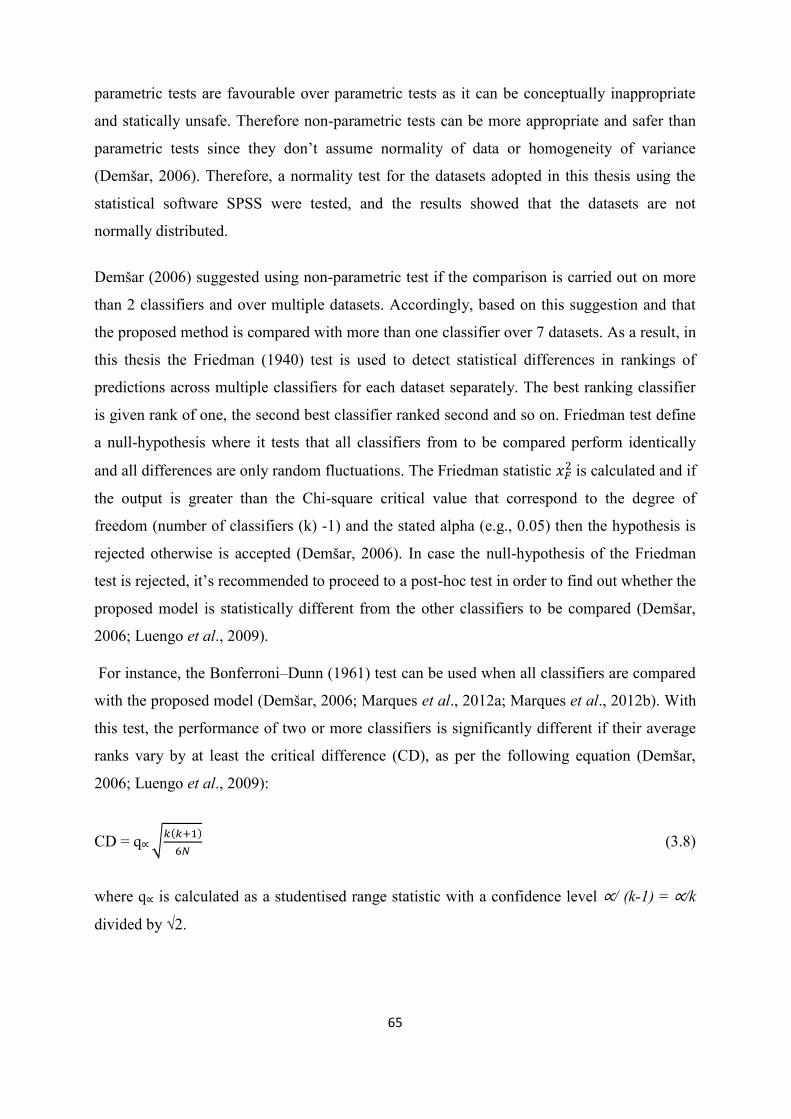
65

parametric tests are favourable over parametric tests as it can be conceptually inappropriate

and statically unsafe. Therefore non-parametric tests can be more appropriate and safer than

parametric tests since they don’t assume normality of data or homogeneity of variance

(Demšar, 2006). Therefore, a normality test for the datasets adopted in this thesis using the

statistical software SPSS were tested, and the results showed that the datasets are not

normally distributed.

Demšar (2006) suggested using non-parametric test if the comparison is carried out on more

than 2 classifiers and over multiple datasets. Accordingly, based on this suggestion and that

the proposed method is compared with more than one classifier over 7 datasets. As a result, in

this thesis the Friedman (1940) test is used to detect statistical differences in rankings of

predictions across multiple classifiers for each dataset separately. The best ranking classifier

is given rank of one, the second best classifier ranked second and so on. Friedman test define

a null-hypothesis where it tests that all classifiers from to be compared perform identically

and all differences are only random fluctuations. The Friedman statistic 𝑥𝐹2‍is calculated and if

the output is greater than the Chi-square critical value that correspond to the degree of

freedom (number of classifiers (k) -1) and the stated alpha (e.g., 0.05) then the hypothesis is

rejected otherwise is accepted (Demšar, 2006). In case the null-hypothesis of the Friedman

test is rejected, it’s recommended to proceed to a post-hoc test in order to find out whether the

proposed model is statistically different from the other classifiers to be compared (Demšar,

2006; Luengo et al., 2009).

For instance, the Bonferroni–Dunn (1961) test can be used when all classifiers are compared

with the proposed model (Demšar, 2006; Marques et al., 2012a; Marques et al., 2012b). With

this test, the performance of two or more classifiers is significantly different if their average

ranks vary by at least the critical difference (CD), as per the following equation (Demšar,

2006; Luengo et al., 2009):

CD = q∝ √𝑘(𝑘+1)

6𝑁 (3.8)

where q∝ is calculated as a studentised range statistic with a confidence level ∝/ (k-1) = ∝/k

divided by √2.

66

3.8 The Proposed Experimental Design Framework

In reference to the all previous discussion, the essential stages of building a comprehensive

credit-scoring model were explained. Garcia et al. (2015) suggested guidelines that need to be

adopted in order to have a rigorous and effective credit-scoring model: 1) Using multiple

dataset, with various sizes. 2) Using an appropriate data splitting technique according to

datasets characteristics. 3) Choose suitable performance evaluation methods that can well

describe the model performance. 4) Carry out appropriate statistical tests in order to validate

the model's performance.

Accordingly, the main experimental design stages of the proposed credit-scoring model

adopted in this thesis can be illustrated in Figure 3.2 As it can be seem from the figure,

several phases and stages make up the experimental design of the proposed model. Therefore,

these stages can be summarised as following:

Stage I: Datasets collection ( 7 datasets are collected to build and validate the model)

Stage II: Pre-processing of the datasets (Cleaning and normalising the dataset).

Stage III: Splitting the datasets (splitting the data for training and testing).

Stage IV: Further processing for the split datasets (feature selection + data-filtering

for the split datasets).

Stage V: Classifiers development and modelling approach (Developing of individual

hybrid and ensemble classifiers).

Stage VI: Performance evaluation measurement for the developed classifiers (Using

different evaluation metrics to assess the classifiers results efficiency).

Stage VII. Statistically test the developed classifiers for their significance (Validate the

classifiers predictions performance statistically).

3.9 Summary

In this chapter, the main stages of the experimental design framework of the proposed model

of this thesis were overviewed. The development of credit-scoring models is a not a simple

practice; it encompasses the collection of datasets and their pre-processing, with the designs

validating and implementing the model. Therefore, the experimental design framework of the

proposed model comprises several essential methods that will lead to a comprehensive and

67

reliable experimental modelling design of a credit-scoring model. In summary, each stage of

the proposed model is fully demonstrated experimentally in the next coming chapters.

Dataset

Missing

Values ?

Data

Replacement

Yes

Data

Normalization

No

Data splitting

Data Filtering

Training

Classifier 1 Classfier i Classfier n

Combining

Classifiers F(x)

Classifiers Performance Evaluation

Significance Tests

Testing

Feature

Selection

Figure 3.2 The main stages of the experimental design for the proposed model

68

CHAPTER 4

CREDIT-SCORING MODELS USING INDIVIDUAL

CLASSIFIERS TECHNIQUES

4.1 Introduction

In this chapter, several methods are used to generate classifiers in order to evaluate their

performance over seven credit datasets. This chapter demonstrates the development of the

individual base classifiers and compare their performance amongst each other to assess the

extent to which the classifiers can perform on different datasets and by using various

evaluation performance metrics. Then, based on the classification results, the need to delve

deeper is justified. In reference to the literature review discussion in Chapter 2 and regarding

the credit classification problem, the 6 most commonly used classification methods in the

literature of credit scoring can be distinguished.

These methods are well-known and are easy to implement, which facilitates banks or credit

cards companies in quickly evaluating the creditworthiness of clients. Therefore, 6 base

classifiers are analysed, namely, NN, SVM, DT, NB, LR and RF. Each of these classifiers has

its own parameters to be set-up based on each dataset. It is worth noting that only the first five

classifiers could be considered as individual classifiers: Inherently, RF is a homogenous

ensemble of many DT but, due to its significantly high performance in credit-scoring field the

decision has been made for it to be included into the group of base classifiers (Lessmann et

al., 2013). LR is served as a benchmark classifier; the objective is to compare results of the

classifiers with performance of LR which serves as the industry standard for credit-scoring

modelling. All the experiments of this thesis are performed using Matlab 2014b version, on a

PC with 3.4 GHz, Intel CORE i7 and 8 GB RAM, using Microsoft Windows 7 operating

system.

69

4.2 Individual Classifiers Development

The most important step of classifier training and development is the selection of its

parameters. In general, credit-scoring datasets vary in their features, and building an effective

scoring model that can deal with different datasets features is crucial. Therefore, in the

training phase, selecting the best parameters for each classifier is very important in order to

evaluate the classifiers and accordingly achieve good performance results. This section will

present: 1) input data to the classifiers has to be prepared and the pre-processed to feed the

classifiers; and 2) the development and training procedure for each selected classifier which

will serve as the base classifiers for the whole proposed developed model in terms of the

classifiers parameters selection and tuning is carried out.

4.2.1 Data Pre-processing and Preparation for Training and Evaluation

Prior to fusing data in to classifiers, data have to be prepared and pre-processed in order to

guarantee the quality of the data and, as a result, improve and ease the knowledge discovery

process of the developed classifiers. In this particular stage, data is pre-processed by:

Imputation of the missing values if occurred in each dataset.

Then the normalisation the input data of each dataset.

Subsequently, data is ready to be partitioned into training and testing set with 10 × 5 cross-

validation. During the training phase, an important stage of classifier-building and

development is conducted, which is selecting and tuning classifiers parameters. Following,

the selected and tuned parameters are used to evaluate and test the performance of the

developed classifiers. The developed classifiers parameters selection and tuning process is

carried out in the next subsection.

4.2.2 Classifiers Parameters Selection and Tuning

All classifiers, with the exception of NB and LR, require parameter selection and tuning.

Moreover, in order to reach optimal results performance, each classifier might have different

parameters depending on the type of dataset evaluated. Below is the description of the

parameters set for each classifier depending on the dataset used. In addition to the description

below a summary of all parameters for all classifiers will be also provided (Please refer to

Appendix A).

70

- NN: The main issue in developing a NN classifier is finding the most suitable

arrangement of learning function, transfer function, training function, learning speed

and the structure topology of the network in terms of number of hidden neurons into

hidden layers so as to solve the classification problem in hand. The developed NN

classifier is based on the back propagation learning algorithm; therefore, various

parameters have been selected and tuned, based on the features of input data. The

transfer function from the hidden layer is chosen to be ′𝑡𝑎𝑛𝑠𝑖𝑔′ the hyperbolic tangent.

This is the most common transfer function used in NN.

𝑡𝑎𝑛ℎ(𝑥) =2

1−𝑒−2𝑥+ 1 (4.1)

As a transfer function from output layer pure linear 'purlin' function was chosen; this means

that single output from a hidden layer does not change but serves as a final decision of NN

classifier. Regarding training functions, many functions are available in Matlab NN Toolbox,

such as trainlm, traingda and traingdx. The purpose of these training functions is to train the

network by updating inputs weights in order to achieve the optimal output value. Besides, for

every particular dataset, it is important to change the way in which the NN is trained: in

German, Australian, Polish, UCSD and Jordanian datasets it stay default (𝑡𝑟𝑎𝑖𝑛𝑙𝑚), whereas

in Japanese and Iranian datasets it change to {𝑡𝑟𝑎𝑖𝑛𝑔𝑑𝑥, 𝑡𝑟𝑎𝑖𝑛𝑔𝑑𝑎} respectively. For the

Japanese dataset a momentum the default parameter of 0.9 was chosen. For all other datasets,

momentum was not defined as 𝑡𝑟𝑎𝑖𝑛𝑙𝑚 and 𝑡𝑟𝑎𝑖𝑛𝑔𝑑𝑎 training methods do not require this

parameter. Regarding the network structure, one hidden layer is used, and the numbers of

neurons in the hidden layers were chosen for reasons of obtained model complexity: the more

neurons in the hidden layer are, the more complex evaluated model is, but in this case training

become much slower and a risk of overfitting may occur. For datasets German, Australian,

Japanese, Iranian, Polish, UCSD and Jordanian the chosen number of neurons in the hidden

layer are {4, 10, 3, 10, 10, 10, 10} respectively. For most of the datasets, value ‘10’ shows the

best performance, but in case of German dataset, NN with only 4 hidden neurons fits input

the best way. Generally, the number of hidden neurons should be chosen relatively to number

and complexity of relations between input features for each dataset. In the developed NN

classifier, a grid search was carried out to find the optimal number of neurons in the hidden

layer for each dataset. The learning rate is default (0.01) in the case of Australian, Japanese,

Iranian, UCSD and Jordanian datasets, while in the German and Polish datasets the values

71

changed to 0.005 and 0.5 respectively. Maximal number of epochs is set to 1000, but almost

always training process finishes by not reaching maximum epoch.

- SVM: The idea of the SVM lies in the basis that if the input data is not linearly

separable lie in moving to a space with higher dimension, in which positive and

negative samples would be linearly separable, this is done by using the kernel

function. The common kernel functions used by SVM can be:

Linear: Linear kernel, meaning dot product.

Quadratic: Quadratic kernel.

Polynomial: Polynomial kernel

RBF: Gaussian Radial Basis Function kernel with has a hyper parameter scaling factor

called sigma.

Throughout the implementing of the SVM classifier, the RBF kernel function was used. For

each dataset, different values of kernel scale parameters were provided (German – ‘1.37’,

Australian, Japanese, UCSD, Polish and Jordanian: 'auto', Iranian: ‘1’). Thus, for the majority

of datasets, the SVM function automatically chooses the appropriate kernel scale. However,

for some datasets, values for the kernel scale parameter that increases SVM Accuracy were

found by grid search in comparison to the default ('auto') parameter.

- RF: The main parameter of the RF classifier is number of trees‍𝑁, 𝑁‍was‍set‍to‍60

based on the best accuracy and computational time on training set. Method used for

RF is 'regression', as it gives better results than default Matlab method. Another

parameter is number of attributes chosen for growing each DT, the default value was

selected (all attributes available in dataset). Another important issue is worth noting is

the defining of the categorical variables for each analysed dataset. Number of the

features which were define as categorical during the RF evaluation is less than initial

number of categorical features because some categorical features is better to consider

as numerical. According to (Rhemtulla et al., 2012) when the categorical variables

have many levels, there is a considerable advantage to treat it as continuous variable.

Let's make an example: in some dataset there is ‘Education’ feature, and ‘0’ means

‘No education’, ‘1’ – ‘ordinary school’, ‘2’ – MSc ‘3’ – ‘PhD’, Here feature can be

considered as numerical, the bigger value of this feature is, the smarter is loan

72

applicant. So during leaf splitting, RF shouldn't iterate over all values of this feature,

but can simply define the leaf threshold, which is more efficient in this case.

- DT: Since different datasets are assessed, and building a DT requires fine-tuning

parameters according to every dataset. For each dataset list of categorical variables is

defined, and passed as a parameter into DT algorithm. Categorical variables are being

estimated separately from the main program. The impurity evaluation is performed

according to Gini’s diversity index. Another option is selecting the algorithm for best

categorical variables split. For two classes, as it is the case, as an optimal was selected

’Exact’ option. That means for categorical variable with C categories, all 2C−1

−1

combinations are considered. After estimating the categorical attributes and defining

additional options the only thing left to be done is to build and execute the tree. After

building the tree, comes the pruning of the tree, pruning is the process of deletion part

of the tree without big decrease of Accuracy. Pruning is used to simplify the model,

and avoid the overfitting. As the available datasets do not have a huge amount of

parameters, pruning was not used after DT training.

4.3 Experimental Results

This section demonstrates the results obtained from each individual base classifier (The

results are evaluated by taking the average of 50 testing sets resulting from the 10 × 5 cross-

validation) across the seven datasets adopted in this thesis. Moreover, six performance

evaluation metrics were used to assess the classifiers performance. After obtaining the results,

all the classifiers across all datasets were compared with the benchmark classifier LR which

is considered the industry standard for credit-scoring modelling to determine the extent to

which the performance of the individual classifiers can be compared to logistic regression.

Table 4.1 show the results of the LR model, Tables 4.2 to 4.6 show the results for the NN,

SVM, RF, DT and NB classifiers, respectively, along with a comparison with the LR in

Figures 4.1 to 4.5. Subsequently, the classifier results obtained are analysed and discussed.

The setup of all classifiers for all datasets is based on the parameters described in previous

section.

73

LR

LR is considered to be a benchmark classifier in this thesis. Table 4.1 demonstrates LR results

across all datasets and for various performance metrics. LR Accuracy for the majority of

datasets is better than NB, DT and NN, but AUC value of NN may be higher than AUC of

LR. On the other hand, LR concedes to RF on all datasets, and sometimes performs worse

than SVM. Brier Score and H-measure of LR are changing accordingly to the Accuracy

(Brier Score is inversely proportional, H-measure is direct proportional), meaning there is no

need to describe them separately. In general, LR is not best, but nonetheless it is a solid

classifier that can be used for fast and quite accurate predictions.

German Australian Japanese Iranian Polish Jordanian UCSD

Accuracy 0.7597 0.8641 0.8626 0.9239 0.7246 0.8240 0.8417

Sensitivity 0.8841 0.8585 0.8474 0.9702 07150 0.9698 0.6439

Specificity 0.4715 0.8700 0.8832 0.0305 0.7325 0.2420 0.9064

AUC 0.7798 0.9294 0.9171 0.6227 0.7405 0.7336 0.8824

Brier Score 0.1656 0.0999 0.1039 0.1005 0.2298 0.1354 0.1144

H-measure 0.2725 0.6352 0.6254 0.0623 0.2663 0.2205 0.4417

Table 4.1 LR results

Figure 4.1 demonstrates the ROC curve of LR across all datasets. In general, LRROC curves

remain RF ones, albeit a bit lower. The three leaders are the Australian, Japanese and UCSD

datasets, whereas other datasets have much lower ROC curves with bad shape.

74

Figure 4.1 LR ROC curve for all datasets

NN

Table 4.2 demonstrates the results of NN across all datasets. In general, the results of the NN

are better than DT and NB in all datasets, and it comes behind RF in all datasets, and it rivals

SVM in most on datasets.

Moreover, as can be seen from Figure 4.2, compared to Logistic Regression, NN shows

worse results across all datasets except in the case of the Iranian dataset (Table 4.2). On the

large dataset UCSD, NN shows a performance that is 1% worse than LR and 3% worse than

RF, but which beats SVM (not by Accuracy, but by AUC and H-measure). Interestingly, for

the Jordanian dataset, NN shows worse results than LR by Accuracy, but better results by

specificity and AUC measure. This means that the NN is more preferable than LR when it is

more important to achieve stability of results for a variety of thresholds and, besides, it is

important to classify bad loans well. This fact describes that the first measure is completely

inadequate in terms of making a decision as to which classifier is better; actually, the decision

75

should be made according to the demands to the predictions and possible threshold and

classifying cost permissible set.

The Brier Score of NN shows similar results as SVM and better average results than LR,

which shows that the certainty of NN is proportional to its output ranking, which can be used

as an additional information during the decision making process.


Accuracy 0.7476 0.8588 0.8581 0.9499 0.6975 0.8148 0.8311

Sensitivity 0.8784 0.8504 0.8466 0.9980 0.6902 0.9352 0.5661

Specificity 0.4440 0.8679 0.8738 0.0120 0.7083 0.3334 0.9176

AUC 0.7638 0.9153 0.9118 0.6132 0.7673 0.7459 0.8590

Brier Score 0.1724 0.1080 0.1078 0.0476 0.1983 0.1423 0.1233

H-measure 0.2390 0.6144 0.6185 0.0615 0.2504 0.2378 0.3978

Table 4.2 NN results

Figure 4.2 NN measures compared to LR

Figure 4.3 shows that NN has the best performance on the Australian and Japanese dataset.

On the UCSD dataset, the ROC curve is a bit lower; however, its perfect shape tells that, for

this dataset, NN can successfully predict good and bad loans for a wide range of thresholds.

-0.0

12

1

-0.0

05

3

-0.0

04

5

0.0

26

0

-0.0

27

1

-0.0

09

2

-0.0

10

6

-0.0

05

7

-0.0

08

1

-0.0

00

8

0.0

29

2

-0.0

24

8

-0.0

34

6

-0.0

77

8 -0

.02

95

-0.0

02

1

-0.0

09

4

-0.0

18

5

-0.0

24

2

0.0

91

4

0.0

11

2

-0.0

16

0

-0.0

14

1

-0.0

05

3

-0.0

09

5

0.0

26

8

0.0

12

3

-0.0

23

4

0.0

06

8

0.0

08

1

0.0

03

9

-0.0

52

9 -0.0

31

5

0.0

06

9

0.0

08

9

-0.0

33

5

-0.0

20

8

-0.0

06

9

-0.0

00

8

-0.0

15

9

0.0

17

3

-0.0

43

9

G E R M A N A U S T R A L I A N J A P A N E S E I R A N I A N P O L I S H J O R D A N I A N U C S D

Accuracy Sensitivity Specificity AUC Brier Score H-measure

76

The German, Jordanian, and Polish datasets ROC curves are almost equal by shape, which

shows that NN is also quite a good classifier for similar datasets. The worst curve that can be

seen is for Iranian dataset.

Figure 4.3 NN ROC curve for all datasets

SVM

Table 4.1 demonstrates SVM results across all datasets and for various performance metrics;

however, several findings can be summarised. Although SVM shows worse Accuracy results

than LR on Australian, Japanese and UCSD datasets, the SVM classifier remains the main

competitor of the RF. All the measures, which are almost the closest to the RF, are not

described here; only special features and big differences.

The Accuracy of SVM differs from RF not more than by 1.45% on the Australian dataset;

however, this difference increases to 2.5% and 3% on the Jordanian and UCSD datasets,

respectively. In fact, SVM gives us less qualitative classification across all datasets, if

comparing with the RF.

77

SVM in general is a very good classifying method; however, regarding SVM, there is a risk

of over-training and/or mis-training over outliers in training data. This is why it is essential to

use filtering, especially with this classifier. SVM performance also decreases in datasets with

high-dimensional input (for example, Iranian and Polish datasets). This is why these datasets

should use feature selection, where such use is more than justified.


Accuracy 0.7614 0.8523 0.8581 0.9482 0.7487 0.8298 0.8306

Sensitivity 0.9118 0.8540 0.8661 0.9980 0.6712 0.9655 0.5060

Specificity 0.4119 0.8498 0.8495 0.0029 0.8211 0.2872 0.9365

AUC 0.7826 0.9109 0.9071 0.6032 0.8206 0.7888 0.8431

Brier Score 0.1659 0.1135 0.1139 0.0505 0.1760 0.1284 0.1341

H-measure 0.2721 0.6024 0.6074 0.0733 0.3655 0.3085 0.3864

Table 4.3 SVM results

Looking at Figure 4.4, SVM beats LR on Iranian, Polish and Jordanian datasets, but it cannot

be crowned as better regarding to the results of Australian and UCSD datasets. As UCSD

dataset is real dataset, it is especially preferably in mind of achieving a good Accuracy on this

dataset; with this task LR performing better than SVM.

Regarding Figure 4.5, it can be seen that SVM, like all other classifiers, has the best

performance on Australian and Japanese datasets. UCSD datasets also should be outlined as

those for which SVM gives pretty good-shaped and high ROC curve. All other datasets are

much worse than these three leaders. The worst Datasets in terms of AUC again is the Iranian

dataset, which its ROC curve lays close to the diagonal. This means that if it is necessary to

significantly increase Specificity for the Iranian dataset, Sensitivity value will drop down till

the level, where classifier performance and results became useless. So, for example, if it is

needed to obtain 50% Specificity value using SVM, Sensitivity value will drop significantly

from 99% to almost 60%, which is considered a completely bad performance.

78

Figure 4.4 SVM measures compared to LR

Figure 4.5 SVM ROC curve for all datasets

0.0

01

7

-0.0

11

8

-0.0

04

5

0.0

24

3

0.0

24

1

0.0

05

8

-0.0

11

1

0.0

27

7

-0.0

04

5

0.0

18

7

0.0

27

8

-0.0

43

8 -0

.00

43

-0.1

37

9

-0.0

59

6 -0

.02

02

-0.0

33

7

-0.0

27

6

0.0

88

6

0.0

45

2

0.0

30

1

0.0

02

8

-0.0

18

5

-0.0

10

0

-0.0

19

5

0.0

80

1

0.0

55

2

-0.0

39

3

0.0

00

3

0.0

13

6

0.0

10

0

-0.0

50

0

-0.0

53

8

-0.0

07

0

0.0

19

7

-0.0

00

4

-0.0

32

8

-0.0

18

0

0.0

11

0

0.0

99

2

0.0

88

0

-0.0

55

3



79

RF

From Table 4.4 it can be inferred that the RF classifier shows the best Accuracy between all

single classifiers on every dataset. Specificity and Sensitivity are the highest when compared

to other classifiers in most cases; however, on Jordanian and UCSD datasets, this rivals with

SVM classifier. On German and Iranian datasets, the Specificity lowers down to 0.44 and

0.056, respectively. The three highest results RF achieves is on Australian, Japanese and

Iranian accordingly. The AUC of the RF classifier, as well as all previous measures, has the

biggest and best results. Being just the best on German, Australian and Japanese datasets, it

stands out on Iranian dataset. Two other measures are much better than other classifiers.


Accuracy 0.7669 0.8668 0.8674 0.9510 0.7625 0.8550 0.8619

Sensitivity 0.9078 0.8685 0.8708 0.9982 0.7548 0.9410 0.6690

Specificity 0.4394 0.8638 0.8640 0.0567 0.7768 0.5131 0.9250

AUC 0.7918 0.9360 0.9308 0.7787 0.8373 0.9087 0.9028

Brier Score 0.1616 0.0947 0.0979 0.0433 0.1646 0.0965 0.1005

H-measure 0.2885 0.6608 0.6485 0.2758 0.3840 0.5345 0.5127

Table 4.4 RF results

The best results between all classifiers may be explained in terms of Probability theory and

good results of the DT classifier. In fact, RF classifier is just a modification of the DT; the

difference lies in the number of decision finding layers. The first layer consists of DT, when

the second is analysing the results of the first layer. The Probability theory prompts: the more

trees you have in your forest, the more weighted and equitable results you achieve. Of course,

the amount of trees should not be infinite; it is easy to get lost with all possible trees. RF is

the only homogeneous ensemble analysed in this chapter, and shows stable and robust results,

meaning it shows a prospects of using this classifier in credit-scoring models.

Figure 4.6 shows RF in comparison with LR across all performance measures. It is clear that

RF beats LR in all measures significantly except the Brier Score and Specificity measure.

80

Figure 4.6 RF measures compared to LR

Regarding Figure 4.7, RF has the best performance on Australian and Japanese dataset. In

general, RF ROC curves are very similar to those of the DT, but they are shifted more so to

the left upper corner, which says that RF is definitely better than the DT. Even for the Iranian

dataset, the ROC curve is only slightly worse than the German dataset. For the Polish dataset,

despite its lower Accuracy, the ROC curve is much higher than German dataset curve.

Therefore, it can be concluded that RF is more efficient (in terms of threshold choosing) for

balanced datasets (like Australian, Japanese and Polish), even if there are many noise and

outliers in them.

0.0

07

2

0.0

02

7

0.0

04

8

0.0

27

1

0.0

37

9

0.0

31

0

0.0

20

2

-0.0

32

1

-0.0

06

2

-0.0

19

2

0.0

26

2

0.0

44

3

0.2

71

1

0.0

18

6

0.0

12

0

0.0

06

6

0.0

13

7

0.1

56

0

0.0

96

8

0.1

75

1

0.0

20

4

-0.0

04

0

-0.0

05

2

-0.0

06

0

-0.0

57

2

-0.0

65

2

-0.0

38

9

-0.0

13

9

0.0

16

0

0.0

25

6

0.0

23

1

0.2

13

5

0.1

17

7

0.3

14

0

0.0

71

0



81

Figure 4.7 RF ROC curve for all datasets

DT

Table 4.5 reveals that the DT classifier is one of the least accurate single classifiers on

German, Australian, Japanese, Polish and UCSD datasets. Although it is the worst classifier,

results on the Jordanian dataset are amongst the best with SVM and RFs. The reason is that

the DT are very sensitive to the number of features, and is inaccurate when it is large. Since

the Jordanian dataset has the least number of features, the DT becomes a good choice. In

regards the Brier score being stable across all datasets, for this dataset, it lowers it down to

0.2665. This could be explained with a higher Accuracy mark. The only measure left is the H-

measure, where the best value has been achieved on datasets but is still the worst compared to

other classifiers.

The DT, by its structure, does not show robust results over multiple training-testing iterations.

This is why it can be seen as relatively bad results on small datasets as Polish, as well as bad

results on complex and big datasets, such as German, Japanese and UCSD. The reason is that

82

building the optimal DT is a NP-complete task, and existing algorithms sometimes fail to

build well-performed DT due to the wrong choice of features. Another reason for the bad

performance of this classifier is he lack of bad loans in training data. Figure 4.8 shows DT in

comparison with LR across all performance measures it can be seen how worse it is compared

to LR except for Brier Score in almost all datasets and Specificity in Jordanian dataset.


Accuracy 0.7045 0.8258 0.8171 0.9238 0.7013 0.8278 0.8201

Sensitivity 0.8001 0.8562 0.8470 0.9641 0.6862 0.8948 0.6178

Specificity 0.4827 0.7886 0.7814 0.1638 0.7177 0.5617 0.8866

AUC 0.6793 0.8664 0.8556 0.6150 0.7278 0.7950 0.7882

Brier Score 0.2521 0.1470 0.1570 0.0698 0.2665 0.1427 0.1586

H-measure 0.1362 0.5153 0.4893 0.1123 0.2097 0.3852 0.3296

Table 4.5 DT results

Figure 4.8 DT measures compared to LR

Regarding Figure 4.9, DT show the best performance on Australian and Japanese datasets. On

Jordanian and UCSD datasets, the results also are good, but are a bit skewed because of these

two datasets and their imbalance. Despite the high Accuracy, the worst curve can be seen is

-0.0

55

2

-0.0

38

3

-0.0

45

5

-0.0

00

1

-0.0

23

3

0.0

03

8

-0.0

21

6

-0.0

84

0 -0

.00

23

-0.0

00

4

-0.0

06

1

-0.0

28

8

-0.0

75

0

-0.0

26

1

0.0

11

2

-0.0

81

4

-0.1

01

8

0.1

33

3

-0.0

14

8

0.3

19

7

-0.0

19

8

-0.1

00

5

-0.0

63

0

-0.0

61

5

-0.0

07

7

-0.0

12

7

0.0

61

4

-0.0

94

2

0.0

86

5

0.0

47

1

0.0

53

1

-0.0

30

7

0.0

36

7

0.0

07

3

0.0

44

2

-0.1

36

3

-0.1

19

9

-0.1

36

1

0.0

50

0

-0.0

56

6

0.1

64

7

-0.1

12

1



83

for Iranian dataset; this may be explained by the fact that Iranian dataset is very skewed.

Figure 4.9 DT ROC curve for all datasets

NB

As shown in Table 4.6, the NB classifiers results on German, Australian, Japanese and

Iranian datasets can rival the DT by the Accuracy measure. On the Jordanian and UCSD

datasets, NB is the least accurate classifier (particularly on UCSD dataset, notably the least

accurate dataset ever for NB). It NB is sensitive to it. As far as it is assumed that features are

independent, some important information may be lost throughout the construction of NBs

model. In fact, NB performance is worse than LR performance in three cases: on large

datasets, on unbalanced datasets, and on datasets with large number of features. Moreover,

since UCSD dataset satisfies all these three conditions, Accuracy of NB classifier compared

to other classifiers drops down very much (see Figure 4.10).

84


Accuracy 0.7250 0.8030 0.7970 0.9262 0.6896 0.8106 0.6140

Sensitivity 0.7639 0.9094 0.9043 0.9622 0.8028 0.9581 0.0553

Specificity 0.6344 0.6707 0.6639 0.2500 0.5880 0.2180 0.7965

Type 1 error 0.2361 0.0906 0.0957 0.0378 0.1972 0.0419 0.9447

Type 2 error 0.3656 0.3293 0.3361 0.7500 0.4120 0.7820 0.2035

AUC 0.7624 0.8962 0.8890 0.7135 0.7401 0.7070 0.5740

Brier Score 0.1994 0.1672 0.1748 0.0755 0.2974 0.1720 0.3143

H-measure 0.2384 0.5802 0.5666 0.1930 0.2346 0.1760 0.0803

Table 4.6 NB results

Figure 4.10 NB measures compared to Logistic Regression

Although NB classifier has the worst value of Sensitivity on Iranian dataset, the Specificity

value is much greater than every other classifier in the German and Iranian dataset. The Brier

Score remains the highest, meaning the worst, but the H-measure concedes only to the NN,

SVM and RF.

As has been stated in the method description, NB classifier assumes that all attributes are

independent of one another, but still able to give very accurate results. It seems clear that real

attributes of a client, whose credit-scoring is being calculated, are never independent. The

ideal Bayes classifier would compute the class without that Naive assumption, calculating the

sought-for probability with each time for each attribute.

-0.0

34

7

-0.0

61

1

-0.0

65

6

0.0

02

3

-0.0

35

0

-0.0

13

4

-0.2

27

7

-0.1

20

2

0.0

50

9

0.0

56

9

-0.0

08

0

0.0

87

8

-0.0

11

7

-0.5

88

6

0.1

62

9

-0.1

99

3

-0.2

19

3

0.2

19

5

-0.1

44

5

-0.0

24

0

-0.1

09

9

-0.0

17

4

-0.0

33

2

-0.0

28

1

0.0

90

8

-0.0

00

4

-0.0

26

6

-0.3

08

4

0.0

33

8

0.0

67

3

0.0

70

9

-0.0

25

0

0.0

67

6

0.0

36

6 0

.19

99

-0.0

34

1

-0.0

55

0

-0.0

58

8

0.1

30

7

-0.0

31

7

-0.0

44

5

-0.3

61

4



85

Regarding to Figure 4.11, NB, not surprisingly, has the best performance on the Australian

and Japanese datasets. On the German dataset it has very solid ROC curve with a good shape.

The ROC curves for all other datasets, with almost all the thresholds lower than ROC curves

of three leaders. For the UCSD dataset, it is worth mentioning that, for some threshold values,

the curve can be seen under the diagonal, from which the conclusion can be drawn that the

Accuracy of NB classifier for the UCSD dataset for some threshold values could be under

50%, which makes no sense, and for these thresholds using NB classifier is completely

unwanted, even on the best possible threshold NB gives around 61%, which is not good at all.

Figure 4.11 NB ROC curve for all datasets

4.4 Analysis and Discussion

Accuracy on the German dataset stands from 70.45% on DT classifier, to 76.76% on RF.

Such low Accuracy, compatible with the percentage of good loans throughout the dataset,

makes the DT not only the poorest classifier on this dataset, but also almost entirely useless

for the classifier, which returns ‘0’ as the prediction in all instances, meaning Accuracy

would be 70%—only half of a percent lower. Specificity and sensitivity differ from classifier

to classifier, but sensitivity mark is always better; this is caused by the ratio of good and bad

86

loans. Although sensitivity and specificity reflect the Accuracy, higher Accuracy does not

mean that both of these measures will rise with the increase of Accuracy. AUC, Brier score

and H-measure also reflect Accuracy, and moreover, this reflection is directly proportional

for AUC and H-measure, and inversely proportional for Brier score for all classifiers.

Australian and Japanese datasets are very similar; the same number of good and bad loans has

very similar attributes and also has similar results, which is why they are described together.

The rating of classifiers differs somewhat to the German dataset: although RF is still the best,

the poorest classifier is now NB with 80.3% on Australian dataset and 79.7% on Japanese

dataset, unlike on the German dataset, where sensitivity and specificity do not depend on the

good/bad loans ratio that much. Although these datasets have more good loans than bad, LR

and NN have bigger specificity than sensitivity. AUC, Brier score and H-measure, as well as

on German dataset, reflect the Accuracy of a classifier. However, NB does not have that

feature, its AUC and H-measure measures are better than some other classifiers, although it

has lower Accuracy.

Regarding the Iranian dataset, the rare situation is when every classifier is if not more

accurate than LR, at the least almost the same (DT). The Iranian dataset, according to

sensitivity and specificity values, shows that the higher Accuracy does not mean that the

classifier is implicitly better. When considering the NN and NB classifiers, NN has a higher

Accuracy but very low specificity, which means that this Accuracy is reached by setting most

of the data to good loans, which provides high accuracy only because of dataset good/bad

loans ratio. NB shows a different situation: the total Accuracy is lower; however, the value of

specificity is much higher. This fact means that, with lower Accuracy, losses of using this

classifier may be less than losses with more accurate classifiers. AUC, Brier score and H-

measure only reflect the Accuracy of each classifier. Only the H-measure of NN shows that

this classifier is strongly trained for one particular mistake price. In terms of Accuracy values,

the Polish dataset is similar to the German dataset; however, the values of the least accurate

classifier, with 68.96% Accuracy, are NB, not the DT, which is still less accurate than the

Logistic Regression. The most accurate classifier remains the RF with 76.25% Accuracy. In

relation to this dataset, there are more bad loans than good ones, which makes the picture of

sensitivity and specificity contrast to the German dataset, meaning, in this dataset, specificity

exceeds sensitivity. The only odd classifier is the NB as the most inaccurate classifier. This,

by far, is the reason behind its in accuracy. AUC, Brier score and H-measure on this dataset,

87

does not reflect Accuracy values that much as on previous datasets; here, situations are

slightly different. On this dataset, the definitions of these measures really matter: for example,

less accurate NN is less dependent from threshold values than more accurate DT. In any case,

RF exceeds every other classifier in every measure.

Regarding the Jordanian dataset, this dataset has 80% good loans, which means that a good

classifier must have an Accuracy equating to higher than 80%. Every classifier on this dataset

reaches this goal, and even the least accurate NB, for example, exceed it for more than 1%.

The sensitivity and specificity ratio reflects the ratio of good/bad loans in the dataset, being at

the same time a good addition to Accuracy. The most accurate classifier on this dataset is RF,

although its sensitivity is not the highest; all those classifiers that have higher sensitivity have,

at the same time, a much lower specificity; in its turn, this lowers classifier Accuracy. In other

words, RF is the most balanced classifier amongst all. In fact, AUC, Brier score and H-

measure are also significantly better than their closest rival, which makes RF an absolute

leader.

A special feature of this dataset is that it consists of unfiltered real-world data. This fact

makes it clear as to why results on this particular dataset differ so much from all obtained

earlier. There is no such dataset, where results would make similar pictures. This influences

every possible classifier and every results measure. Accuracy, for example, has an average

value of 84%, if not counting NB, the accuracy of which constitutes only 61.4%. In the

description of NB, it is said that it is assumed that all of the data features are independent

from one another. If on other datasets it could work, this assumption here causes the

Accuracy, which is even worse if it is said that all of the loans in the dataset are bad. In actual

fact, NB is close to that, as far as its sensitivity is ten times lower than the other closest one.

Other classifier measures are proportional. Now, with all results obtained, it is desirable to

improve these results and decide which classifier can be considered the best.

To decide, let us look at the Accuracy comparison diagrams. They clearly show that the most

common classifier Logistic Regression, with no doubt, wins every other classifier on

Australian and Japanese datasets, except in the case of the RF. On Polish dataset, it rivals

with SVM and RF; however, the difference is less than 0.4 %, so on these datasets the

decision of the best classifier comes down to personal preferences. On Australian, Japanese

and Iranian, the most desirable classifier seems to be one of SVM, RF or NN. The use of NB

88

and DT on these three datasets is unwarranted; their Accuracy is much lower than the

proposed classifiers. To conclude, the commonness of LR classifier is clearly reasoned with

its higher Accuracy on most possible datasets. There is no grounding in changing the

classifier until it becomes better than LR on those datasets where it concedes. Looking on the

comparing figures for all classifiers, one can conclude that LR is one of the best classifiers,

slightly worse than RF, and for some datasets SVM. LR shows convincing results on

Australian, Japanese and UCSD datasets Australian, Japanese and UCSD, and slightly worse

results on German dataset. LR is a solid classifier, which works well on the data with a lot of

features and possible inaccuracies. Table 4.7 summarize the best classifiers in term of their

accuracies.

Accuracy German Australian Japanese Iranian Polish Jordanian UCSD Average Rank

RF 1 1 1 1 1 1 1 1

SVM 2 4 3.5 3 2 2 4 2.9

LR 3 2 2 5 3 4 2 3

NN 4 3 3.5 2 5 5 3 3.6

DT 6 5 5 6 4 3 5 4.9

NB 5 6 6 4 6 6 6 5.6

Table 4.7 Rankings of base classifiers based on their accuracy across all datasets

One trend suggested in this thesis to improve the classifiers all at once is to enable sample or

instance filtering and feature selection. Sample filtering is an algorithm which finds the

exceptions (outliers) within the training data set. Feature selection dedicates which features

do not influence the result that much to be paid attention. These two methods might change

the situation in favour of other classifiers. Sample filtering and feature selection Accuracy

improving are the topic of the next chapter.

4.5 Summary

In this chapter, six state-of-the art individual base classifiers adopted in this thesis were

demonstrated. A total of seven credit datasets were used to validate the classifiers and six

performance measures were used to evaluate their performance: first the data was pre-

proceeded and normalised; second, they were partitioned into training and testing sets using

10 x 5 cross-validations; and thirdly, classifiers’ parameters were tuned on training datasets in

89

order to achieve the optimal value; and finally, classifiers were ready to be evaluated, with the

final results found to be the average of 50 runs.

The classifier results have been developed with LR used as a benchmark classifier to be

compared with the rest of the classifiers in order to determine the extent to which classifiers’

results perform against the industry standard LR. Results vary from classier to classifier, with

the RF showing the best performance across all classifiers and across all datasets,

emphasising superiority over logistic regression, with SVM beating LR in some cases.

In the next chapter, the various hybrid approaches are used in order to enhance the

performance of the model and to determine the extent to which complex modelling enhances

the performance over individual classifiers, as well as over the industry LR.

90

CHAPTER 5

CREDIT-SCORING MODELS USING HYBRID


5.1 Introduction

The target of the previous chapter was centred on the application of the state-of-the art

classification techniques individually and the assessment of their performance. This chapter

seeks to minimise the risks and accordingly improve the Accuracy over the individual

classifiers by implementing the hybrid approaches, such as data-filtering and feature selection

for classifiers. The rationale behind the feature selection is the idea that removing

unimportant or Accuracy-understating features from the classifier arguments list will improve

the classifier's Accuracy. The second method, filtering, is used to improve the results of

machine-learning classifiers, which obviously should be trained on some training data before

applying to testing entries. Filtering algorithm improves the training set of data by removing

the inaccurate samples from the set. Inaccurate data samples are those that stand out from the

whole picture: for example, an object of sample data stands all between the good samples, but

the label of this sample is ‘bad’. In this case, such an object would be removed from the

training set.

This chapter describes the data-filtering and feature selection algorithms and developing

hybrid classifiers using these two approaches. After all, using obtained results, classifiers are

compared comprehensively in terms of using feature selection and data-filtering separately

and by combining them together; up to our best knowledge, combining data-filtering

techniques with feature-selection techniques has not been considered before in the area of

credit-scoring. Finally, the decision has been made that hybrid classifiers with filtering and

feature selection together are better than considering them separately as well as applying

classifiers individually. The results are compared to the industry standard LR and see the size

of the improvement when used over individual classifiers.

91

5.2 Data-Filtering

As discussed in Chapter 3, the idea of the Gabriel Neighbourhood Graph editing (GNG) is

used as a filtering algorithm, the idea of the GNG algorithm is based on the idea of proximity

graphs which consist of a set of vertices and edges such that any two data points are

connected if they satisfy some neighbourhood relations (Garcia et al., 2012). Hence, the main

motivation of selecting GNG algorithm and proximity graphs is as following:

Proximity graphs are used to avoid incoherentnes of data (when some places are full

of points and some places have only few points).

Proximity graphs find neighbors in each direction, so if some point has two neighbors,

one and another just behind the first, the second will not count. This fact is unlike k-

NN filtering, where directions of neighbors don’t count.

Proximity graph describe the structure of data very well, so for each point the

algorithm finds the closest matches to it.

The efficient way to reflect structure of the data and interconnection between training set

entries is to represent training data using graph structure. The simplest way is to connect two

data points when they are close enough. So 𝑥𝑖 and 𝑥𝑗 are connected if 𝑑(𝑥𝑖. 𝑥𝑗) < 𝜖, where 𝜖 is

chosen manually). This method is easy but using this method in the case of non-uniform data

distribution it is impossible to derive coherency of data representation: some graph areas is

full of edges, but other areas will have a few edges. Moreover, it is not guaranteed that

obtained graph is connected. Thus, another idea is to use proximity graphs, which are

building without using fixed distance 𝜖, but connects two data points regarding of their

neighbours location with respect to them. So, the Gabriel Neighbourhood graphs (GNG)

(Garcia et al., 2012) were used as a special case of proximity graphs to get a list of

neighbours for each point from the training set.

The idea behind data-filtering is the selection of the data outliers, data points which labels are

weakly suit to the labels of its neighbours, so it can be assumed that some mistake in data

collection or representation was made and this data point may contain an error. Thus, the best

way is not to include such data into training process. Now, let 𝑑(⋅.⋅) be the Euclidean distance

in 𝑅𝑛. The GNG is defined as follows:

(𝑥𝑖, 𝑥𝑗) ∈ 𝐸 ⇔ 𝑑2(𝑥𝑖, 𝑥𝑗) ≤ 𝑑

2(𝑥𝑖, 𝑥𝑘) + 𝑑2(𝑥𝑗, 𝑥𝑘), ∀𝑥𝑘, 𝑘 ≠ 𝑖, 𝑗 (5.1)

92

Figure 5.1 demonstrate the connection between 2 points in the GNG, in simple words, the

idea is to connect the points 𝑖 and 𝑗 if and only if there is no point 𝑘 inside the circle with

segment [𝑖. 𝑗] as a diameter, otherwise the 2 point will not be connected. Euclidian distance is

calculated as follows: given two points 𝑥𝑖 = (𝑥𝑖1. 𝑥𝑖2. 𝑥𝑖3. … ) and 𝑥𝑗 = (𝑥𝑗1. 𝑥𝑗2. 𝑥𝑗3. … )

Euclidean distance can be calculated as follows:

𝑑(𝑥𝑖. 𝑥𝑗) = √(𝑥𝑖1 − 𝑥𝑗1)2+ (𝑥𝑖2 − 𝑥𝑗2)

2+⋯+ (𝑥𝑖𝑛 − 𝑥𝑗𝑛)

2 (5.2)

Figure 5.1 Illustration of GNG edge connection (Gabriel & Sokal, 1969)

Figure 5.2 illustrate the construction of a GNG on a 2-D training dataset and show how points

are connected and the process of filtering data points depending on meeting certain conditions

by the GNG algorithm.

Figure 5.2 Construction of a Gabriel Neighbourhood Graph for a 2-D training dataset (Gabriel & Sokal, 1969)

93

As it can be seen from Figure 5.2, the GNG is constructed and training data points are

connected, now for each sample 𝑥∗ the weighted average for all neighbour labels to 𝑥∗ are

evaluated. In this case the weights chosen are proportional to the distance from each 𝑥∗. Also

for every data point two scalar values, T0 and T1 are defined that can be interpreted as

thresholds. Subsequently, two conditions are checked whether:

If label of 𝑥∗ equal to 0, and weighted average of all GNG is greater than T0, 𝑥∗ is

removed or filtered from training set.

If label of 𝑥∗ equal to 1, and weighted average of all GNG is less than T1, 𝑥∗ is removed or

filtered from training set.

If neither condition is satisfied, 𝑥∗will remain in the training set.

In balanced datasets, where number of '0' labels is approximately equal to number of ‘1’

labels, it is wise to use 0.5 as both T0 and T1 thresholds. But in the case of imbalanced

datasets, when number of bad loans is far less than number of good loans, values of both

thresholds equal to 0.5 leads to excessive filtration for entries with data labelled as ‘1’.

Therefore the proposed new enhancement on the GNG in this thesis is using the following

two approaches:

Using weighted average for GNG instead of simple average in order to find to count far

points less than close points for each 𝑥∗‍to more precisely find outliers.

Using various thresholds to avoid excess filtering of bad loan entries in case the datasets

are imbalanced.

For clear understating the steps of the GNG filtering algorithm is summarised in the

following pseudo-code:

1. Compute GNG for all entries from training set:

For every pair 𝑥𝑖 𝑥𝑗 from training set:

- Check whether to connect them in GNG using Equation (5.1).

End for

2. For each classifier optimal good loans and bad loans thresholds (𝑇𝑟0, 𝑇𝑟1) are

evaluated beforehand.

94

For each entry 𝑥𝑖 of training set

- Compute the vector 𝑙 which consists of actual labels of all 𝑥𝑖 Gabriel Graph

neighbours.

- Compute the vector 𝑤 which consists of distances from 𝑥∗ to its Gabriel Graph

neighbours.

- Perform consequently such operations: 𝑤 = max(𝑤) − 𝑤,

- Evaluate𝑙∗ = 𝑤 ⋅ 𝑙, where ⟨⋅⟩ is a scalar product of vectors.

- If label of 𝑥∗ equal to 0, and 𝑙∗ is greater than 𝑇𝑟0, 𝑥∗ is removed from training set.

- If label of 𝑥∗ equal to 1, and 𝑙∗ is less than 𝑇𝑟1, 𝑥∗ is removed from training set.

End for

3. Perform training stage of selected classifier over reduced training set.

For illustration purposes the steps can be demonstrated in the following 2-D graphs (x-axis:

could be any variable in a dataset, y-axis: is the loan decision) presented in Figure 5.3.

a. Initial training data

95

b. Building GNG using this training Data

c. Filtering entries which satisfy filtering conditions

Figure 5.3 Example of filtering process on a 2-D dataset

Figure 5.3 the process of filtering for a sample 2-D dataset of labelled points is clearly

demonstrated. The first sub-graph is the initial training set before filtering. The second sub-

graph demonstrates proximity GNG built over the training dataset. The red circles around the

dots means that according to the GNG filtering algorithm they is filtered out. The third sub-

graph demonstrates the result of filtering algorithm. The black and blue crosses are placed in

the positions of the points that were filtered out from the training set and the reaming points

are trained. After applying the GNG filtering algorithm on the training set of the 7 datasets of

this thesis across the 5 base classification algorithms, the percentages of the filtered training

data for each dataset across the several base classifiers are illustrated in Table 5.1.

96

Dataset NN SVM RF DT NB Average % of

filtered data

German 1.4% 3.3% 1.4% 13.3% 14.1% 6.7%

Australian 6.67% 8.7% 12.1% 10% 11.44% 9.782%

Japanese 14.2% 10.43% 4.5% 10.29% 10.43% 9.97%

Iranian 0.5% 0.9% 0.5% 4.9% 0.5% 1.46%

Polish 15.4% 28.7% 1.7% 32.9% 22% 19.74%

Jordanian 4.8% 4.8% 17.8% 17.8% 3% 9.64%

UCSD 5.75% 2.83% 0.45% 5.75% 15.23% 6.00%

Average %

of filtered

data

6.96% 8.52% 5.49% 13.56% 10.96% 9.04%

Table 5.1 Filtered percentages of training data for all classifiers and datasets

Table 5.1 clearly shows that dataset with the biggest rate of filtered data is the Polish dataset,

and dataset with the lowest rate of filtered data is the Iranian dataset. In general, it can be

concluded that the more the dataset is balanced, the higher the rate the data could be filtered

out (e.g., Australian, Japanese and Polish datasets). However, by choosing thresholds T0 and

T1 different levels of filtered data can be obtained, but what is interesting, that the most

efficient levels are bigger for balanced datasets. This can be explained, by the fact, that for

imbalanced datasets it’s not efficient to filter out too many data of minor class, as training set

can become even more imbalanced, which, in general can badly affect the training process.

Regarding the data of major class, this is difficult to choose the right threshold to avoid

filtering out any important and valuable data points.

Classifiers which gave the best results with high level of filtered data are DT and NB, which

can be easily explained by the structure of these classifiers. Classifiers which need low level

of filtering are RF and NN. RF gives good results even without filtering, because this

classifier use voting ensemble of DT, and even if some of them make wrong decision due to

outlier data points, majority of other DT correct the prediction. Regarding the NN, it is well

known that feedforward NN is stable with respect to noisy and incorrect data if the level of

the noise and errors isn’t too big.

In the next section results of the base classifiers across all datasets using the GNG filtering

algorithm is summarised.

97

5.2.1 Classifiers Results Using the GNG filtering algorithm

Tables 5.2 to 5.6 summarise and discuss the results of the 5 base classifiers across 7 datasets

evaluated on six performance measures (The results are evaluated by taking the average of 50

testing sets resulting from the 10 × 5 cross-validation). All the base classifiers is hybridized

by applying the GNG filtering algorithm in order to filter the training data from noisy and

outlier instances and deliver to the classifiers a new training set.

NN

According to Table 5.2 the changes of the NN are in general are insignificant. NN, on the

training phase, adjusts its weights to minimise mean-squared error at the output. Thus, even if

some inputs are incorrect or outliers, the majority of good entries will overcome bad entries,

thus NN will train properly. But with some datasets filtering makes results of NN much better

(e.g., Polish dataset), because this dataset has noisier data than others (19.74% in average,

according to Table 5.1). So NN backpropagation procedure fails to deals with such big

number of bad entries, and Accuracy of NN became low.


Accuracy 0.7507 0.8588 0.8654 0.9488 0.7433 0.8198 0.8400

Sensitivity 0.8570 0.8224 0.8626 0.9984 0.7016 0.9317 0.5712

Specificity 0.5025 0.9030 0.8695 0.0065 0.7859 0.3733 0.9273

AUC 0.7663 0.9161 0.9077 0.6132 0.8058 0.7649 0.8573

Brier Score 0.1728 0.1095 0.1091 0.0481 0.1839 0.1368 0.1182

H-measure 0.2461 0.6233 0.6302 0.0703 0.3361 0.2685 0.4207

Table 5.2 NN results using GNG filtering algorithm

SVM

Table 5.3 demonstrates that SVM with data-filtering is better than without data-filtering.

However, the reason of the slight increase in Accuracy of the SVM classifier after filtering

implementing lay in the problem of impossibility to build the perfect separating hyper plane.

During the construction of this hyper plane, some of the samples are being filtered by the

classifier itself: If good and bad loans are not linearly separable, the number of ignorable

samples depends on the separating-in Accuracy parameter of soft-margin SVM algorithm.

98


Accuracy 0.7677 0.8626 0.8533 0.9464 0.7558 0.8342 0.8324

Sensitivity 0.8976 0.8494 0.8066 0.9958 0.6901 0.9603 0.5159

Specificity 0.4667 0.8786 0.9123 0.0095 0.8151 0.3285 0.9356

AUC 0.7956 0.9210 0.9113 0.6491 0.8095 0.8241 0.8442

Brier Score 0.1642 0.1050 0.1112 0.0508 0.1772 0.1191 0.1349

H-measure 0.2961 0.6356 0.6219 0.1166 0.3648 0.3859 0.3971

Table 5.3 SVM results using GNG filtering algorithm

RF

Table 5.4 shows the stability of RF results with and without filtering and this could be

explained by the nature of the RF itself. The classifying results of the RF classifier depend not

only on the training inputs fed into it, but also on the number and parameters of its members

the DT. RF implicitly filters the training input data by itself, and filtering algorithm does not

change the result of its work a lot. The best Accuracy RF demonstrates on the Australian and

the Iranian dataset, however the best values of AUC and H-measure classifier shows for

Japanese dataset. For the UCSD dataset RF demonstrates solid results, only a bit worse than

the results for the best two datasets.


Accuracy 0.7698 0.8677 0.8667 0.9508 0.7521 0.8638 0.8679

Sensitivity 0.8965 0.8734 0.8492 0.9979 0.7632 0.9682 0.6884

Specificity 0.4757 0.8596 0.8893 0.0587 0.7500 0.4486 0.9266

AUC 0.7927 0.9228 0.9292 0.7876 0.8344 0.8892 0.9155

Brier Score 0.1608 0.1006 0.0985 0.0430 0.1669 0.0998 0.0949

H-measure 0.2939 0.6475 0.6493 0.3010 0.3751 0.5138 0.5410

Table 5.4 RF results using GNG filtering algorithm

DT

The results of Table 5.5 absolutely show that all performance measures of DT classifier were

improved with filtering, only the Accuracy on Iranian dataset is an exception as it can be

explained by the huge imbalance of this dataset (There is a big risk to filter out some bad loan

entries that are useful for training process. As there is only 5% of bad loan entries, all filtered-

99

out bad loan entry increases the imbalance of Iranian dataset even more). The most significant

raise amongst all measures can be noticed on AUC and H-measure characteristic. This can be

explained by the fact, that filtering process often decreases the imbalance of dataset, so

classifier results became more robust with respect to threshold and misclassification cost

changing. Regarding to Brier Score, this characteristic also increased a lot: the filtering

algorithm allows selecting the most accurate subset of the training data, making the classifier

more certain about its correct predictions, which could be considered as useful improvement.


Accuracy 0.7446 0.8677 0.8635 0.9505 0.7513 0.8526 0.8343

Sensitivity 0.8874 0.8683 0.8425 1.0000 0.7380 0.9414 0.5776

Specificity 0.4143 0.8655 0.8896 0.0117 0.7666 0.4997 0.9182

AUC 0.6890 0.8876 0.8822 0.5303 0.7701 0.7630 0.7796

Brier Score 0.2301 0.1216 0.1274 0.0491 0.2338 0.1323 0.1503

H-measure 0.1815 0.6150 0.6068 0.0363 0.3115 0.3541 0.3444

Table 5.5 DT results using GNG filtering algorithm

NB

As well as DT classifier's results, Table 5.6 show that NB results also are increasing after

data-filtering. However, the reason of this improvement is that the filtering improves the

distribution of the input training data, so if the normal distribution were used as as a

parameter of NB classifier, this assumption became more close to the truth. Moreover,

filtering increases the confidence of the classifier that is why the Brier Score also performed

very well, indicating the NB is more confidence in its own decisions.


Accuracy 0.7590 0.8649 0.8630 0.9307 0.7262 0.8134 0.8069

Sensitivity 0.8680 0.8696 0.8579 0.9676 0.8800 0.9614 0.7317

Specificity 0.5052 0.8581 0.8702 0.2376 0.5904 0.2189 0.8314

AUC 0.7747 0.9109 0.9085 0.7224 0.7733 0.7101 0.8231

Brier Score 0.1981 0.1203 0.1221 0.0707 0.2637 0.1746 0.1908

H-measure 0.2675 0.6240 0.6225 0.2107 0.3021 0.1848 0.3730

Table 5.6 NB results using GNG filtering algorithm

100

5.3 Feature Selection

As discussed in Chapter 3, the main aim of feature selection is to choose an optimal subset of

features for improving prediction Accuracy or decreasing the size of the structure without

significantly decreasing prediction Accuracy of the classifier built using only the selected

features. This type of data pre-processing is important for many classifiers as it increases

learning speed and Accuracy over testing set. To fulfil this purpose MARS technique is used

to determine the most valuable variables or features over the input data. MARS is widely

accepted by researchers and practitioners for the following reasons (Lee et al. 2002) and that

is why it is adopted in this thesis:

MARS is capable of modeling complex non-linear relationship among variables

without strong model assumptions.

MARS can evaluate the relative importance of independent variables to the dependent

variable when many potential independent variables are considered.

MARS does not need long training process and hence can save lots of model building

time, especially when working with a large dataset.

Resulting model can be easily interpreted.

After finishing the training stage, the obtained MARS is as a mathematical generalised linear

model, which fits the data well. But this model can be used not only to classify entries, but to

analyse the input data and find the most important features, which are highly correlated with

target labels. The aim of feature selection is to choose a subset of features for improving

prediction Accuracy or decreasing the size of the structure without significantly decreasing

prediction Accuracy of the classifier built using only the selected features. This type of pre-

processing method is important for many classifiers as it increases learning speed and

Accuracy over testing set. ANOVA decomposition is used over MARS mathematical model

to determine the most valuable and important features over the input data. The main

characteristic which distinguishes MARS from other classifiers is that result of MARS

classifier is easily-interpreted model, and then ANOVA can be used with this model to make

investigations of input data structure, particularly feature importance. ANOVA, obviously,

cannot be used without MARS, and the results depend on how well MARS classifier is

trained.

According to (Wood et al, 1997) ANOVA decomposition is summarised by one row for each

MARS hinge function or product of these functions. Not all columns of ANOVA table are

101

used, only the second one, which gives the standard deviation of the function. This gives one

indication of its relative importance to the overall model and can be interpreted in a manner

similar to a standardized regression coefficient in a linear model. Each hinge function inside

ANOVA table commonly responds to one feature, so the values of the second column are

taken as an importance vector for all features. But if hinge function consists of 𝑁 features, and

there is some value 𝐴 in the second column, then value to each of the features is added, that

constitute this hinge function. The relative importance of each feature is computed by

computing MARS for all iterations and afterwards evaluating ANOVA decomposition. For

each iteration the second column of the ANOVA table is stored, and then at the end of the

whole algorithm all these columns are mixed into the single one by computing the average

value of each position for all columns. The steps of MARS feature selection process can be

summarised in Pseudo-code as following:

1. Suppose there are 𝑁 iterations, for each of them dataset is divided to training and

testing parts.

For i from 1 to N do

Evaluate MARS algorithm over training set with given parameters:

- Maximum number of functions in the model allowed. The default value for this

parameter is -1 in which case maxFuncs is calculated automatically using

formula‍𝑚𝑖𝑛(200.𝑚𝑎𝑥(20. 2𝑑)) + 1‍(Jekabsons, 2016), where d is the number of input

variables.

- Penalty value per knot. Larger values leads to fewer knots being placed (i.e., final

models is simpler)

- Perform ANOVA decomposition of obtained model using 𝑎𝑟𝑒𝑠𝑎𝑛𝑜𝑣𝑎 function. Store

second column of this table as (𝑖) . Thus, 𝑤𝑘(𝑖) denotes importance of k-th input

feature during i-th iteration.

End For

2. Assume 𝑁𝑓 is total number of features of the data.

For s from 1 to 𝑁𝑓 do

𝑤𝑠 =∑ ‍𝑁𝑖=1𝑤𝑠(𝑖)

𝑁 (5.3)

End for

102

3. Return 𝑤 = (𝑤1. 𝑤2. …𝑤𝑁𝑓)

4. Suppose that for each single classifier optimal feature importance threshold 𝑇𝑖𝑚𝑝 was

evaluated beforehand. Thus, for training and testing only features 𝑖 are chosen, for

which 𝑤𝑖 > 𝑇𝑖𝑚𝑝

As part of analysis of feature selection algorithm, the number of features that are filtered out

from each dataset by each classifier is demonstrated in Table 5.7.

Datasets All features NN SVM RF DT NB

German 20 16 18 16 12 12

Australian 14 12 12 13 12 9

Japanese 15 15 15 15 12 15

Iranian 27 21 13 21 18 13

Polish 30 20 20 23 10 22

Jordanian 12 8 8 10 8 7

UCSD 38 15 16 38 15 15

Table 5.7 Number of selected features

The obtained figures in Table 5.7 clearly show that Australian and Japanese datasets are the

two datasets that retain most of their features (only 2-3 features were removed). On the other

hand, for Iranian and Polish datasets, features reduced massively (up to 20 features, in the for

DT for Polish dataset). Some of the classifiers such as RF or NN are more resistant to a large

number of features, that is why their results are high enough even with all features selected.

Conversely, classifier as DT is very vulnerable to datasets with high amount of features. SVM

in general is more stable to redundant features, but computational complexity of building

optimal separating hyper plane in case of large-dimensional input space also increases a lot.

Another thing worth mentioning is that MARS feature selection algorithm assigned '0'

importance to 6 features on Iranian dataset, the reason is that Iranian dataset is highly

imbalanced, that is why MARS computed very simple model in that case without these 6

features. Tables 5.7 to 5.13 illustrate weights of each of the dataset features

German dataset

Feature # 1 2 4 5 3 6 10 14 7 9 11

Weight 6.06 3.98 3.58 3.48 3.46 2.74 2.13 1.75 1.65 1.64 1.62

Feature # 15 8 20 13 12 19 17 16 18

Weight 1.56 1.43 1.42 1.14 1.13 0.45 0.42 0.14 0.02

Table 5.8 Features importance for German dataset

103

Australian dataset

Feature`s # 8 10 5 3 14 7 4 13 12

Weight 13.47 3.72 3.66 3.52 3.14 2.59 2.33 2.06 1.49

Feature # 6 2 9 1, 11

Weight 0.36 0.34 0.06 0.00

Table 5.9 Features importance for Australian dataset

Japanese dataset

Feature # 5 4 9 11 3 15 6 8 14

Weight 17.77 16.08 14.06 3.81 3.35 3.28 2.67 2.46 2.15

Feature # 7 2 1 10 13 12

Weight 1.10 0.22 0.14 0.09 0.08 0.02

Table 5.10 Features importance for Japanese dataset

Iranian dataset

Feature # 1 8 3 19 21 6 9 4 2

Weight 2.82 1.64 1.12 1.09 1.06 0.88 0.71 0.62 0.54

Feature # 24 5 26 14 25 10 23 20 7

Weight 0.17 0.15 0.13 0.13 0.07 0.06 0.06 0.06 0.05

Feature # 13 11 27 12, 15, 16, 17, 18, 22

Weight 0.05 0.04 0.04 0.00

Table 5.11 Features importance for Iranian dataset

Polish dataset

Feature # 22 21 30 6 13 18 10 5 23

Weight 26.01 23.02 12.87 12.34 8.49 7.57 3.72 3.70 3.08

Feature # 1 4 24 17 14 15 3 2 19

Weight 2.96 2.67 2.59 2.52 2.50 2.41 2.31 1.74 1.43

Feature # 9 25 8 7 12 27 26 11, 16, 20, 28, 29

Weight 0.93 0.64 0.41 0.23 0.11 0.06 0.06 0.00

Table 5.12 Features importance for Polish dataset

104

Jordanian dataset

Feature # 8 9 6 5 10 3 1 7 11 2 4

Weight 14.69 10.34 7.42 5.00 4.19 4.03 1.07 0.79 0.44 0.37 0

Table 5.13 Features importance for Jordanian dataset

UCSD dataset

Feature # 32 13 33 28 37 19 24 29 8

Weight 7.28 6.07 3.78 3.60 3.28 2.34 2.15 1.98 1.55

Feature # 11 27 17 26 30 2 18

1, 3, 4, 5, 6, 7, 9, 10, 12, 14,

15, 16, 20, 21, 22, 23, 25,

31, 34, 35, 36, 38

Weight 1.52 1.09 0.68 0.25 0.19 0.12 0.03 0.00

Table 5.14 Features importance for UCSD dataset

Tables 5.8–5.14 illustrate the importance of each feature in each dataset. As it can be seen,

many features were weighted high that reflect its importance and some very low which reflect

it uselessness. Also it can be noticed that the more features dataset has, the more of them

appear to be unnecessary. The best example of it can be observed in the Iranian and the

UCSD datasets. These are real world datasets, include a lot of information collected while

deciding to loan grant a loan or not and it seems that it only stores space and rarely make

difference in decisions.

105

5.3.1 Classifiers Results Using MARS

Tables 5.15 to 5.19 summarise and discuss the results of the 5 base classifiers across 7

datasets evaluated on 6 performance measures (The results are evaluated by taking the

average of 50 testing sets resulting from the 10 × 5 cross-validation). All the base classifiers

obtained results are based on applying MARS algorithm to compute the most important and

valuable features for each classifier on each dataset.

NN

According to Table 5.15, on the most of datasets, the Accuracy of the NN classifier rises up,

but for some of them Accuracy remains the same and even slightly decrease (e.g., German

and Iranian datasets). In general, NN results are stable against redundant and unimportant

features, so the small rise of NN Accuracy can be considered as a success, even if for some

datasets this rise is slight. Other NN measures change accordingly, and often the rise of other

measures is even more than Accuracy rise (as for German dataset, where Accuracy remains

almost the same, but AUC increases by 0.32%)


Accuracy 0.7475 0.8649 0.8617 0.9494 0.6892 0.8382 0.8473

Sensitivity 0.8719 0.8584 0.8515 0.9991 0.6622 0.9326 0.6503

Specificity 0.4602 0.8720 0.8756 0.0037 0.7203 0.4589 0.9120

AUC 0.7670 0.9193 0.9110 0.6180 0.7715 0.8265 0.8889

Brier Score 0.1706 0.1040 0.1079 0.0478 0.1960 0.1209 0.1112

H-measure 0.2479 0.6289 0.6188 0.0609 0.2592 0.3775 0.4659

Table 5.15 NN results using MARS

SVM

In this case, Table 5.16 shows the fact that the SVM classifier becomes better with feature

selection is not a surprise. The fewer number of features used means that the points which are

used in separating have fewer dimensions to be considered. This in its turn simplifies the

process of building a separating hyper plane.

106


Accuracy 0.7655 0.8525 0.8575 0.9483 0.7538 0.8368 0.8444

Sensitivity 0.9153 0.8618 0.8692 0.9981 0.6844 0.9447 0.6336

Specificity 0.4178 0.8401 0.8444 0.0029 0.8199 0.4107 0.9134

AUC 0.7827 0.9051 0.9075 0.5655 0.8257 0.7960 0.8742

Brier Score 0.1647 0.1138 0.1143 0.0508 0.1731 0.1238 0.1393

H-measure 0.2807 0.5963 0.6077 0.0379 0.3744 0.3734 0.4558

Table 5.16 SVM results using MARS

RF

As well as the filtering effect, Table 5.17 shows the effect of feature selection algorithm is

mostly positive, but insignificant. This can be easily explained by the fact that RF consists of

several DT, and each has different features included. So if the number of RF DT members is

big enough, we'll definitely have a bunch of DT with the best Accuracy, which have only

important features included, so if number of insignificant features is less than 20-30%, these

will push DT to make a right decision. The reasons of classifier stability with feature

selection are the same as its stability with filtering.

Although the Accuracy for some datasets has dropped down slightly, the drop was not more

than tenths of a percent, which can be considered as statistically insignificant. Moreover, with

almost the same Accuracy, most of other measures (e.g., AUC and H-measure) show a slight

rise.


Accuracy 0.7667 0.8680 0.8662 0.9507 0.7679 0.8616 0.8664

Sensitivity 0.9031 0.8703 0.8694 0.9976 0.7638 0.9418 0.6793

Specificity 0.4499 0.8647 0.8628 0.0609 0.7776 0.5457 0.9376

AUC 0.7869 0.9403 0.9317 0.7896 0.8417 0.9203 0.9136

Brier Score 0.1628 0.0928 0.0976 0.0434 0.1624 0.0922 0.0960

H-measure 0.2835 0.6678 0.6509 0.2783 0.3950 0.5671 0.5375

Table 5.17 RF results using MARS

107

DT

Looking at Table 5.18, unlike with the RF, the results of DT change a lot with the

implementation of feature selection algorithm. The improvements are mostly positive; the

only exception is the Accuracy on the Japanese dataset which drop is little. The reason of the

general increment in the DT can be is in computation complexity of building the optimal DT

as it grows exponentially with respect to number of features. For example, if the number of

features increases by 10, optimal DT will compute 1000 times slower. That is why DT

growing Matlab algorithm allows computational simplification and that is why it often builds

non-optimal DT. Thus, the reason that results are increased comparing with classical DT

classifier is similar to the case of enabling filtering. Each decision which node to divide and

how to do that with presence of redundant features have the risk to be incorrect.


Accuracy 0.7212 0.8275 0.8167 0.9268 0.7254 0.8304 0.8544

Sensitivity 0.8198 0.8553 0.8444 0.9664 0.7179 0.8967 0.6319

Specificity 0.4924 0.7933 0.7837 0.1805 0.7344 0.5690 0.8875

AUC 0.6924 0.8676 0.8568 0.6394 0.7532 0.8092 0.8006

Brier Score 0.2392 0.1462 0.1563 0.0676 0.2412 0.1366 0.1521

H-measure 0.1561 0.5180 0.4929 0.1514 0.2637 0.4023 0.3497

Table 5.18 DT results using MARS

NB

In Table 5.19 and in comparing to the first experiment Chapter 4, where NB was trained

without data pre-processing, much better results with feature selection can be seen. The

increase is the most obvious on a dataset with large amount of features (e.g., Iranian, Polish

and UCSD datasets). In this experiment the features, which their impact on the entry label is

minimal, are removed from training and testing data, so they have no opportunity to affect

classifier's decision in the bad way. On the other hand, for Japanese dataset the Accuracy does

not change, which is explained by the fact, that all features for NB classification were

considered as important.

It is worth mentioning, that for UCSD dataset results of NB became better, but it remains the

worst classifier with 62.5% Accuracy. So for large real-world datasets using such simple

108

classifiers with only feature selection and without other powerful pre-processing techniques is

not a good idea.


Accuracy 0.7437 0.7849 0.7970 0.9447 0.7071 0.8210 0.6253

Sensitivity 0.8469 0.9202 0.9043 0.9866 0.7477 0.9875 0.0459

Specificity 0.5043 0.6161 0.6639 0.1555 0.6734 0.1540 0.8147

AUC 0.7678 0.8944 0.8890 0.7397 0.8011 0.7094 0.5930

Brier Score 0.1858 0.1735 0.1748 0.0547 0.2569 0.1692 0.3063

H-measure 0.2463 0.5739 0.5666 0.2181 0.3391 0.1771 0.0967

Table 5.19 NB results using MARS

5.4 Classifiers Results Using GNG + MARS

The previous experiments in this chapter were conducted on applying both GNG filtering

algorithm and MARS feature selection on the base classifiers independently. Different results

were obtained; this section combines both GNG filtering algorithm and MARS feature

selection to see to what extent results can be enhanced. Consequently, Tables 5.20 to 5.24

summarise and discuss the results of the 5 base classifiers across 7 datasets evaluated on 6

performance measures, followed by comparison with LR in Figures 5.4 to 5.8 (The results are

evaluated by taking the average of 50 testing sets resulting from the 10 × 5 cross-validation).

Results are compared to the results of previous experiments, and assumptions are made of

how and why filtering and feature selection affect various measures differently for different

classifiers. Moreover, the results are compared to the industry standard LR and assess to what

extent classifier results with hybrid modelling can outperform LR.

NN

In NN results as in Table 5.20, the Accuracy for almost all datasets increases with

implementing of GNG and MARS methods. The exact method, which causes positive

changes, depends on a dataset, but together they always show the best result. Actually, NN

does feature selection by itself implicitly: the principal of NN says that while learning, the

network assigns the proper weight to each feature. If a feature is not considered as important,

in NN, with or without feature selection, it does not influence the result. So external feature

selection (what is been conducted in this chapter) on NN should not give significant

109

advantage. However, looking at the results and by applying feature selection, some datasets

results increased (e.g., Jordanian and UCSD datasets). The reason of this that external feature

selection removes features completely from the consideration, so if some feature applied to

the input of NN, anyway it will have some impact, as weights from this feature are very

unlikely to be all ‘0’ at the same time. That is why sometimes feature selection improves the

results of NN very much.

Sensitivity and Specificity change on every classifier in the same way. Absolutely the same

thing could be said about other three performance measures. The NN algorithm by itself

should not be very sensitive to redundant features and noisy outlier data. But indeed, the

performance of NN shows advantage and importance of using filtering and feature selection

as a pre-processing algorithm. The highest improvements are on Polish, Jordanian and UCSD

datasets. Hence, this combination shows improvements on all 7 datasets.


Accuracy 0.7584 0.8643 0.8694 0.9500 0.7521 0.8454 0.8487

Sensitivity 0.8680 0.8584 0.8689 0.9994 0.7200 0.9325 0.6047

Specificity 0.5069 0.8713 0.8713 0.0127 0.7850 0.4994 0.9285

AUC 0.7717 0.9197 0.9073 0.6289 0.8060 0.8348 0.8825

Brier Score 0.1700 0.1035 0.1092 0.0472 0.1838 0.1193 0.1101

H-measure 0.2580 0.6313 0.6309 0.0747 0.3406 0.4042 0.4634

Table 5.20 NN results using GNG + MARS

As in Figure 5.4, with filtering and feature selection NN becomes a good alternative to the

LR, showing better Accuracy on every dataset except German, and on this dataset it concedes

on 0.1 percent, which is statistically insignificant difference. On average NN performance is

in general better than LR in 4 datasets on the other four measures, So, on the datasets like

these, NN shows solid results, stable against threshold and misclassifying cost change.

110

Figure 5.4 NN measures compared to Logistic Regression

The improvement of ROC curves of NN can be seen on all datasets except the Japanese,

although this decrease can be caused by random fluctuations, thus it is considered as

statistically insignificant. It can be concluded that filtering and feature selection improves the

classifiers performance on all datasets (see Figure 5.5).

Figure 5.5 NNROC curve for all datasets

-0.1

3%

0.0

2%

0.6

8%

2.6

1%

2.7

5%

2.1

4%

0.7

0%

-1.6

1%

-0.0

1%

2.1

5%

2.9

2%

0.5

0%

-3.7

3%

-3.9

2%

3.5

4%

0.1

3%

-1.1

9%

-1.7

8%

5.2

5%

25

.74

%

2.2

1%

-0.8

1%

-0.9

7%

-0.9

8%

0.6

2%

6.5

5%

10

.12

%

0.0

1%

0.4

4%

0.3

6%

0.5

3%

-5.3

3%

-4.6

0%

-1.6

1%

-0.4

3%

-1.4

5%

-0.3

9%

0.5

5%

1.2

4%

7.4

3%

18

.37

%

2.1

7%

G E R M A N A U S T J A P A N E S E I R A N I A N P O L I S H J O R D A N I A N U C S D


111

SVM

In Table 5.21 and regarding to the filtering and feature selection, the Accuracy of SVM

changes contrarily on different datasets. On German, Australian, Polish, Jordanian and UCSD

datasets it raises, but on other two datasets it decreases. It is unexpected, because the

reduction is caused by filtering, and filtering should conversely improve the Accuracy,

simplifying the separating hyper plane. SVM is the only classifier which the impact of feature

selection is more than data-filtering.

Sensitivity, Specificity and other measures change according to Accuracy changes for each

dataset. The other thing is that feature selection gives more impact on SVM results than

filtering, while for all other classifiers situation is exactly opposite. It can be concluded that

SVM is very sensitive to the redundant features.


Accuracy 0.7733 0.8686 0.8538 0.9464 0.7571 0.8474 0.8455

Sensitivity 0.9038 0.8667 0.8069 0.9959 0.7024 0.9424 0.6362

Specificity 0.4703 0.8703 0.9129 0.0082 0.8080 0.4705 0.9140

AUC 0.7942 0.9209 0.9111 0.6123 0.8158 0.8300 0.8683

Brier Score 0.1643 0.1043 0.1112 0.0508 0.1749 0.1133 0.1433

H-measure 0.2985 0.6370 0.6215 0.0784 0.3700 0.4585 0.4548

Table 5.21 SVM results using GNG + MARS

Figure 5.6 clearly shows that SVM got higher results on average than LR on all datasets,

except Japanese dataset. For Jordanian dataset, SVM shows much better AUC and H-

measure, so for Jordanian dataset from these two measures exactly SVM should be chosen as

more robust against threshold and misclassifying cost change. For the Australian dataset all

measures of SVM are better, except for AUC.

112

Figure 5.6 SVM measures compared to Logistic Regression

Figure 5.7 shows that SVM is the only classifier whose ROC curves are roughening instead

of smoothening, however the overall picture becomes better, all the figures become closer to

upper left point, which means becoming better a priori. The ROC curve for the Jordanian

dataset has one of the best results, which means that in most cases SVM classifier might work

better with the real data than with classical testing data.

Figure 5.7 SVM ROC curve for all datasets

1.3

6%

0.4

5%

-0.8

8%

2.2

5%

3.2

5%

2.3

4%

0.3

8%

1.9

7%

0.8

2%

-4.0

5%

2.5

7%

-1.2

6%

-2.7

4%

-0.7

7%

-0.1

2%

0.0

3%

2.9

7%

-2.2

3%

7.5

5%

22

.85

%

0.7

6%

1.4

4%

-0.8

5%

-0.6

0%

-1.0

4%

7.5

3%

9.6

4%

-1.4

1%

-0.1

3%

0.4

4%

0.7

3%

-4.9

7%

-5.4

9%

-2.2

1%

2.8

9%

2.6

0%

0.1

8%

-0.3

9%

1.6

1%

10

.37

%

23

.80

%

1.3

1%



113

RF

According to Table 5.22, the results of RF are enhanced by combining both GNG and MARS

methods. The improvement of the RF results due to filtering is based on the idea of the

filtering itself, for example some of the samples do not help to train the classifier properly as

they lie too close to the samples of the opposite class. Without inaccurate samples the error

became lower and Accuracy rises. Feature selection also helps to reduce number of features,

that’s why DT of the RF are built more precisely and optimally. However, the improvement is

smaller than for other classifiers, and this fact was explained in previous sections, where

analysed results were analysed with filtering and feature selection separately.

Specificity and Sensitivity change differently, the raise of both measures only could be found

in the Polish dataset, but on the rest of measures if one has increased, the second has

necessarily decreased. These increases and decreases do not exceed 0.2 % and can be

explained by the fact, that RF Accuracy changes only a bit, and thus ROC curve changes

insignificantly. Here and further, if such tendency reveals itself in other classifiers results, it

could be explained by the fact that optimal point of ROC curve. When the ROC curve slightly

increases, the optimal point of it changes too, what causes changes in Sensitivity and

Specificity.

The reduction of the Brier Score is simply explained by the Accuracy and the H-measure

increasing. Although feature selection and filtering are insufficient when applied separately,

but together they increase the Accuracy quite noticeably. However, this increase is not

enough to say that RF becomes much better with feature selection and filtering.


Accuracy 0.7725 0.8707 0.8717 0.9513 0.7742 0.8669 0.8690

Sensitivity 0.9066 0.8799 0.8806 0.9985 0.7782 0.9669 0.6924

Specificity 0.4611 0.8585 0.8618 0.0555 0.7774 0.4655 0.9269

AUC 0.7942 0.9286 0.9293 0.7786 0.8408 0.8861 0.9162

Brier Score 0.1603 0.0982 0.1001 0.0430 0.1627 0.1006 0.0946

H-measure 0.2966 0.6491 0.6513 0.2831 0.3945 0.5027 0.5422

Table 5.22 RF results using GNG + MARS

114

Regarding Figure 5.8, just as it was without filtering and feature selection, RF classifier stays

more accurate than LR on every dataset. The Accuracy increases by 3.9% on Australian

dataset and by 1.1% on Jordanian dataset. All measures of RF stay higher than corresponding

measures of LR The only exception is in Specificity in datasets German, Australian and

Japanese datasets, but balance between these two values (Specificity and Sensitivity) can be

easily adjusted by changing threshold value. As soon as AUC of RF is bigger than AUC of

LR, with changed threshold this advantage is maintained. Also Brier Score for RF is

improved across all datasets.

Figure 5.8 RF measures compared to Logistic Regression

Figure 5.9 shows that the ROC curves with feature selection and filtering combined become

smoother in comparison with ROC curves of RF from the previous chapter. This means that

classifier becomes more balanced, although the AUC values decrease in all cases except

Polish and UCSD datasets. The decrease of AUC, as it is known, means decrease the ability

of classifier to work with a wide range of thresholds, however if classifier demonstrates high

rise of Accuracy, relative small decrease of AUC can be considered as insignificant.

1.2

8%

0.6

6%

0.9

1%

2.7

4%

4.9

6%

4.2

0%

2.7

3%

2.2

5%

2.1

4%

3.3

2%

2.8

3%

6.3

2%

-0.2

9%

4.8

5%

-1.0

4%

-1.1

5%

-2.1

4%

2.5

0%

4.4

9%

22

.35

%

2.0

5%

1.4

4%

-0.0

8%

1.2

2%

15

.59

%

10

.03

% 15

.25

%

3.3

8%

-0.5

3%

-0.1

7%

-0.3

8%

-5.7

5%

-6.7

1%

-3.4

8%

-1.9

8%

2.4

1%

1.3

9%

2.5

9%

22

.08

%

12

.82

%

28

.22

%

10

.05

%



115

Figure 5.9 RFROC curve for all datasets

DT

It can be clearly seen from Table 5.23 that the results of DT increased comparing to results in

the previous chapter; however, according to Figure 5.10 on German and Japanese datasets

this raise is not enough to beat the LR. AUC value of DT is also smaller than corresponding

value of LR, this can be easily explained by the values of predictions that DT can produce as

output, majority of the DT output predictions are either ‘0’ or ‘1’, and only small fraction of

these predictions lies between these two values. That’s why, its ROC curves have a shape

more similar to triangle, than ROC curves of other classifiers, and this is the reason why AUC

value is lower than the AUC values of classifiers with similar Accuracy. Brier score and H-

measure on majority of datasets are also lower than LR.

As well as on RF, the Accuracy of DT has also increased, and on Polish dataset it improved

up to 4%. This increase is caused mostly by data-filtering, and slightly by feature selection. In

this case, filtering allows to weight every decision more accurately, when the feature selection

only tries to remove the attributes from classification process, that have only slight influence

on a label of the data, the set of features is originally are redundant so some of them cannot be

116

considered as important. The situation with the Sensitivity, Specificity, AUC, Brier Score and

H-measure is completely same to RF, as well as its background. Feature selection and

filtering improve the results of the DT separately, and together the improve they cause is even

better.


Accuracy 0.7528 0.8688 0.8616 0.9505 0.7900 0.8612 0.8414

Sensitivity 0.8964 0.8653 0.8434 1 0.7516 0.9444 0.5960

Specificity 0.4204 0.8722 0.8847 0.0117 0.8279 0.5295 0.9216

AUC 0.6994 0.8868 0.8795 0.5362 0.7975 0.7809 0.7933

Brier Score 0.2214 0.1216 0.1292 0.0489 0.2027 0.1248 0.1424

H-measure 0.1973 0.6157 0.6025 0.0400 0.3818 0.3994 0.3735

Table 5.23 DT results using GNG + MARS

Figure 5.10 DT measures compared to Logistic Regression

In Figure 5.11, ROC curves of the DT with the influence of filtering and feature Selection

become more linear. On the Iranian dataset, the curve is parallel to the random line. Other

shifts of the curves are due to datasets proportion of good and bad loans in dataset, the more

dataset is imbalanced, the more figure shifts, and the Iranian dataset is the best example of

this. An opposite conclusion is also possible, the more balanced the dataset is, the better ROC

-0.6

9%

0.4

7%

-0.1

0%

2.6

6%

6.5

4%

3.7

2%

-0.0

3%

1.2

3%

0.6

8%

-0.4

0%

2.9

8%

3.6

6%

-2.5

4%

-4.7

9%

-5.1

1%

0.2

2%

0.1

5%

-1.8

8%

9.5

4%

28

.75

%

1.5

2%

-8.0

4%

-4.2

6%

-3.7

6%

-8.6

5%

5.7

0%

4.7

3%

-8.9

1%

5.5

8%

2.1

7%

2.5

3%

-5.1

6%

-2.7

1%

-1.0

6%

2.8

0%

-7.5

2%

-1.9

5%

-2.2

9%

-2.2

3%

11

.55

% 1

7.8

9%

-6.8

2%



117

curve it has, although in this particular case the most balanced dataset the Polish comes after

the Australian and Japanese datasets due to its big number of features.

Figure 5.11 DT ROC curve for all datasets

NB

According Table 5.24, the situation with NB Accuracy is a bit different from DT and RFs. In

general, the NB performance improved Japanese dataset Accuracy comes in the third place in

Accuracy after RF and NN. However, on Iranian dataset the Accuracy stays almost the same

comparing with experiment with MARS and without GNG (0.9452 with this experiment and

0.9447 in the experiment with Feature Selection and without filtering).

However, the Accuracy of NB with only filtering is only 0.9307. The possible explanation for

this might lie in filtering. Iranian dataset consists of very small number of bad loans, and each

bad loan is surrounded by good loan points. So filtering while deleting bad loan entries

degrade bad/good loans proportion, the feature selection also has its weak sides; algorithm

might have considered some features as unimportant, what, in combination with naive

assumption that the attributes are independent, caused reduction of the Accuracy on this

dataset. On other measures, the only difference from the already examined measures is the

118

rise of AUC. This gives a good evidence to say that, for now, only NB becomes more

universal.


Accuracy 0.7638 0.8614 0.8630 0.9452 0.7296 0.8212 0.8083

Sensitivity 0.8861 0.8420 0.8579 0.9881 0.9038 0.9852 0.7787

Specificity 0.4789 0.8844 0.8702 0.1328 0.5775 0.1642 0.8181

AUC 0.7735 0.9093 0.9085 0.7470 0.7996 0.7765 0.8312

Brier Score 0.1927 0.1249 0.1221 0.0537 0.2642 0.1574 0.1908

H-measure 0.2668 0.6149 0.6225 0.2373 0.3449 0.2587 0.3958

Table 5.24 NB results using GNG + MARS

In Figure 5.12 and comparing to LR results, NB shows negative performance. Only on

Iranian dataset the performance of this classifier is better. On Polish dataset Accuracy is a bit

better, but most of other measures, including AUC is slightly better. On real-life UCSD

dataset NB shows lower result than LR, but comparing to the results with GNG and MARS,

NB shows tremendous rise in Accuracy (from 61.4% to almost 81%).

Figure 5.12 NB measures compared to Logistic Regression

According to Figure 5.13, ROC curves give only more evidence to the conclusion that GNG

and MARS soften the ROC curve for all datasets. This can be explained by the fact that NB

0.4

1%

-0.2

7%

0.0

4%

2.1

3%

0.5

0%

-0.2

8%

-3.3

4%

0.2

0%

-1.6

5%

1.0

5%

1.7

9%

18

.88

%

1.5

4%

13

.48

%

0.7

4%

1.4

4%

-1.3

0%

10

.23

%

-15

.50

%

-7.7

8%

-8.8

3%

-0.6

3%

-2.0

1%

-0.8

6%

12

.43

%

5.9

1%

3.9

9%

-5.1

2%

2.7

1%

2.5

0%

1.8

2%

-4.6

8%

3.4

4%

2.2

0%

7.6

4%

-0.5

7%

-2.0

3%

-0.2

9%

17

.50

%

7.8

6%

3.8

2%

-4.5

9%



119

ROC curves on datasets with lower number of features have good shape (and thus AUC have

bigger value). That's why ROC curves on datasets with high number of features improve due

to GNG and MARS applied. Thus, the best results are on datasets Australian and Japanese,

whereas the best improvement could be seen on the UCSD dataset, which is amongst the

most affected datasets by MARS. Other dataset's ROC curves in this case come very close to

each other near the optimal value of threshold, which means similar results in the wide range

of thresholds for all of them.

Figure 5.13 NB ROC curve for all datasets

5.5 Comparison of Results and Justification of Combining GNG + MARS

In this section an evaluation is conducted on the Accuracy improvement for all single

classifiers depending of pre-processing algorithms being used. For each classifier a table is

presented which demonstrates advantage of using GNG + MARS in combination. Tables 5.25

to 5.29 demonstrate an extensive comparison on individual classifiers based on:

All data and features.

All features and filtered data by GNG method.

All data and just important features selected by MARS.

120

Filtered data by GNG method and important features selected by MARS.

All increases represent the Accuracy change comparing to individual classification, with all

data and features. The advantage of filtering and feature selection pre-processing algorithms

combination is clearly seen in row 7 of all tables, when comparing to row 3 and row 5.

NN

Below in Table 5.25 GNG+MARS communicate in very special way. It could be said that

GNG and MARS alone work differently. Both methods together improve the Accuracy for all

datasets especially from 0.01% on Iranian dataset and to 5.46% on Polish dataset.


Individual

classification 0.7476 0.8588 0.8581 0.9499 0.6975 0.8148 0.8311

GNG 0.7507 0.8588 0.8654 0.9488 0.7433 0.8198 0.8400

Increment after

implementing

GNG 0.31% 0% 0.73% -0.11% 4.58% 0.5% 0.89%

MARS 0.7475 0.8649 0.8617 0.9494 0.6892 0.8382 0.8473

Increment after

implementing

MARS -0.01% 0.61% 0.36% -0.05% -0.83% 2.34% 1.62%

GNG + MARS 0.7584 0.8643 0.8694 0.9500 0.7521 0.8454 0.8487

Increment after

implementing

GNG+MARS 1.08% 0.55% 1.13% 0.01% 5.46% 3.06% 1.76%

Table 5.25 NN results comparison of GNG, MARS and GNG+MARS

SVM

According to Table 5.26, shows SVM the most controversial classifier, although

GNG+MARS should improve the Accuracy, the result looks different for the Japanese and

Iranian datasets. However, MARS on Japanese dataset decrease the Accuracy more than that

in GNG because Japanese dataset does not have many features, comparing to the Polish

dataset, for example. Finally, the way GNG and MARS work together is good as the overall

increase is a little greater than increase of applying pre-processing methods separately.

121


Individual

classification 0.7614 0.8523 0.8581 0.9482 0.7487 0.8298 0.8306

GNG 0.7677 0.8626 0.8533 0.9464 0.7558 0.8342 0.8324

Increment after

implementing

GNG 0.63% 1.03% -0.48% -0.18% 0.71% 0.44% 0.18%

MARS 0.7655 0.8525 0.8575 0.9483 0.7538 0.8368 0.8444

Increment after

implementing

MARS 0.41% 0.02% -0.06% 0.01% 0.51% 0.7% 1.38%

GNG + MARS 0.7733 0.8686 0.8538 0.9464 0.7571 0.8474 0.8455

Increment after

implementing

GNG+MARS 1.19% 1.63% -0.43% -0.18% 0.84% 1.76% 1.49%

Table 5.26 SVM Results comparison of GNG, MARS and GNG+MARS

RF

Table 5.27 shows a good example of how GNG+MARS work jointly better than separately.

This is clear on the Japanese dataset, where Accuracy decreases by 0.07% and 0.12% with

GNG and MARS respectively, but by combining them the Accuracy increases by 0.43%.


Individual

classification 0.7669 0.8668 0.8674 0.9510 0.7625 0.8550 0.8619

GNG 0.7698 0.8677 0.8667 0.9508 0.7521 0.8638 0.8679

Increment after

implementing

GNG 0.29% 0.09% -0.07% -0.02% -1.04% 0.88% 0.06

MARS 0.7667 0.8680 0.8662 0.9507 0.7679 0.8616 0.8664

Increment after

implementing

MARS -0.02% 0.12% -0.12% -0.03% 0.54% 0.66% 0.45%

GNG + MARS 0.7725 0.8707 0.8717 0.9513 0.7742 0.8660 0.8690

Increment after

implementing

GNG+MARS

0.56% 0.39% 0.43% 0.03% 1.17% 1.1% 0.71%

Table 5.27 RF Results comparison of GNG, MARS and GNG+MARS

122

Also a rare case is represented on Polish dataset, when filtering decreases the Accuracy and

feature selection increases it. The reason it goes this way is that Polish dataset has the less

number of data samples and the large number of features.

DT

Like on the RF, Table 5.28 here demonstrates GNG+MARS work well together. Both of them

separately increase the Accuracy, but combining them increase the Accuracy in all datasets

accept the Japanese, where GNG alone is better than GNG + MARS, this might be because of

MARS performance alone where it was worse than the Individual classification. Also another

massive increment for both methods is on Polish dataset where the increment is 8.87% which

is better the both methods separately.


Individual

classification 0.7045 0.8258 0.8171 0.9238 0.7013 0.8278 0.8201

GNG 0.7446 0.8677 0.8635 0.9505 0.7513 0.8526 0.8343

Increment after

implementing

GNG 4.01% 4.19% 4.64% 2.67% 5.00% 2.48% 1.42%

MARS 0.7212 0.8275 0.8167 0.9268 0.7254 0.8304 0.8244

Increment after

implementing

MARS 1.67% 0.17% -0.04% 0.30% 2.41% 0.26% 0.43%

GNG + MARS 0.7528 0.8688 0.8616 0.9505 0.7900 0.8612 0.8414

Increment after

implementing

GNG+MARS 4.83% 4.30% 4.45% 2.67% 8.87% 3.34% 2.13%

Table 5.28 DT Results comparison of GNG, MARS and GNG+MARS

NB

According Table 5.29, the use of GNG +MARS work the same way as on DT, for all datasets

increment is more than using them separately except on the Australian dataset where GNG

alone is better. In General, the performance of GNG alone is quite good with NB. But when

combining with MARS the performance gets better if the MARS performance is better than

Individual classification (e.g., Australian and Japanese datasets).

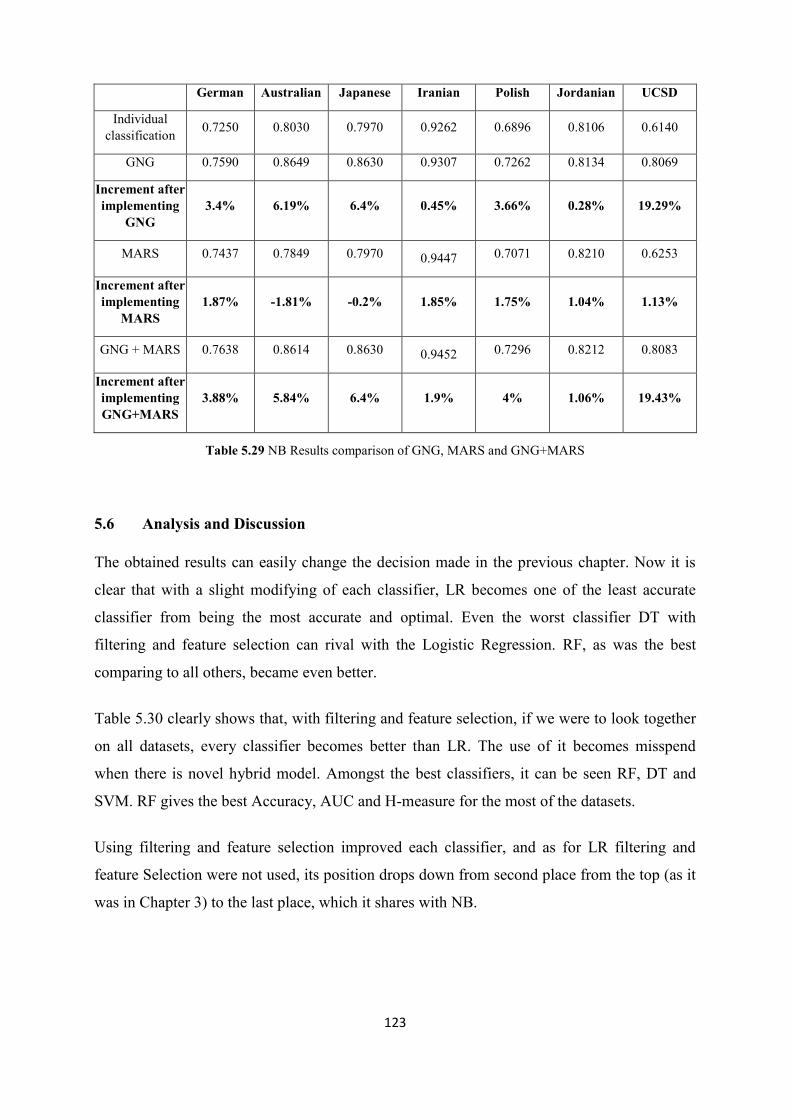
123


Individual

classification 0.7250 0.8030 0.7970 0.9262 0.6896 0.8106 0.6140

GNG 0.7590 0.8649 0.8630 0.9307 0.7262 0.8134 0.8069

Increment after

implementing

GNG 3.4% 6.19% 6.4% 0.45% 3.66% 0.28% 19.29%

MARS 0.7437 0.7849 0.7970 0.9447 0.7071 0.8210 0.6253

Increment after

implementing

MARS 1.87% -1.81% -0.2% 1.85% 1.75% 1.04% 1.13%

GNG + MARS 0.7638 0.8614 0.8630 0.9452 0.7296 0.8212 0.8083

Increment after

implementing

GNG+MARS 3.88% 5.84% 6.4% 1.9% 4% 1.06% 19.43%

Table 5.29 NB Results comparison of GNG, MARS and GNG+MARS


The obtained results can easily change the decision made in the previous chapter. Now it is

clear that with a slight modifying of each classifier, LR becomes one of the least accurate

classifier from being the most accurate and optimal. Even the worst classifier DT with

filtering and feature selection can rival with the Logistic Regression. RF, as was the best

comparing to all others, became even better.

Table 5.30 clearly shows that, with filtering and feature selection, if we were to look together

on all datasets, every classifier becomes better than LR. The use of it becomes misspend

when there is novel hybrid model. Amongst the best classifiers, it can be seen RF, DT and

SVM. RF gives the best Accuracy, AUC and H-measure for the most of the datasets.

Using filtering and feature selection improved each classifier, and as for LR filtering and

feature Selection were not used, its position drops down from second place from the top (as it

was in Chapter 3) to the last place, which it shares with NB.

124

Accuracy German Australian Japanese Iranian Polish Jordanian UCSD Average Rank

RF 2 1 1 1 2 1 1 1.29

DT 6 2 5 2 1 2 5 3.29

SVM 1 3 6 4 3 3 3 3.29

NN 5 4 2 3 4 4 2 3.43

NB 3 6 3 5 5 6 6 4.86

LR 4 5 4 6 6 5 4 4.86

Table 5.30 Rankings of base classifiers based on their accuracy across all datasets

Now let us show how much results have increased during applying these GNG and MARS

methods together (in average by all datasets):

NB: 6.07%

DT: 4.37%

NN: 2.41%

SVM: 0.90%

RF: 0.63%

It can be seen, that the worse results classifier shows without filtering and feature selection,

the best improvement can be seen after applying these two pre-processing methods. So let us

make a receipt when using filtering and feature selection is extremely useful:

When the dataset is well-balanced.

When data have a lot of features and some of them are categorical.

When any individual classifiers without filtering and feature selection give surprisingly

low results, which cannot be explained by other reason than existing of outliers in data.

When DT or NB used as a part of classification system. Even if one of them can be

applied to the data being analysed, using filtering and feature selection in combination is

very desirable.

Finally, it is very important to mention and describe the thresholds assigned to GNG + MARS

to each classifier for each dataset (Please refer to Appendix B).

125

5.7 Summary

In Chapter 2, the approaches are introduced namely GNG and MARS methods which are

data-filtering and feature selection techniques respectively. Several experiments were carried

out in order to build hybrid models with better Accuracy. Data-filtering and feature selection

were applied separately and in combination in order to see different effects on classifiers

results.

After applying GNG and MARS, relative and absolute performance of all classifiers without

an exception changed a lot. The most sensitive classifiers to these techniques are DT and NB

classifiers. Accuracy of NB increased by 6% in average, the most change was for the UCSD

dataset. Accuracy of DT increased by 4.3%, which also is very good; on the other hand, RF is

the least sensitive classifier to filtering and feature selection, the reason of this lies is an in the

complex structure of this classifier, which by itself consists of a bunch of random DT, as well

as initially high results of RF even without filtering and feature selection. As it can be seen

from comparison tables, filtering and feature selection in combination almost gives for

classifiers higher result comparing to experiments with applying only one of these techniques.

The main conclusion can be conducted from this chapter is that using filtering and feature

selection in combination is justified, and the experiments conducted with these two pre-

processing techniques show major improvement for all classifiers, comparing to non-pre-

processing and one pre-processing technique. It is worth noting, that filtering is more

responsible for Accuracy increase than feature selection. This can be seen when the results of

experiments were compared with only filtering and feature selection applied separately. Thus

the logical question come up into mind, whether is it feasible to combine the predictions of all

five classifiers so the performance of their combination is higher? In the next chapter simple

combiners is considered, with the hope that it will help to obtain higher results. (This is next

step in the direction of creating a perfect classifier, called the consensus classifiers approach,

which is discussed in the Chapter 7). So different experiments is carried out to use several

simple combiners, which is described in details in the next chapter and combine them using

simple multi-argument functions as MIN, MAX, PROD, AVG etc. amongst all traditional

combiners the best and the worse is addressed and suggestions is made on which combiner is

better to use in which situations.

126

CHAPTER 6

CREDIT-SCORING MODELS USING ENSEMBLE


6.1 Introduction

Whilst there is a bunch of single classifiers with a good performance, the question on how to

use their predictions together in order to obtain the most accurate predictions still remains

open. The most common way to merge single classifiers predictions is to use simple

function‍𝑓(𝑥1. 𝑥2. 𝑥3. 𝑥4. 𝑥5) = 𝑥∗, which convert all single classifiers predictions 𝑥𝑖 into

actual output ranking. An important issue in combining classifiers is that it is particularly

useful if they are different, see (Kittler et al., 1998). This can be achieved using different

feature sets or selecting different subsets of training data (Xu et al., 1992; Kuncheva, 2004).

In the previous two chapters, the principles of single classifiers and the methods reviewed

which improved their Accuracy with data-filtering and feature selection were demonstrated.

The next step in their analysis is to examine how they work together, building an ensemble of

single classifiers with a more complex ensemble classifier in a result. In fact, the ensemble is

just a classifier, whose arguments are the results of all single member classifiers. There are a

lot of different ways how the ensemble could work, but here are the ones, which are

implemented in this thesis:

Min Rule (MIN)

Max Rule (MAX)

Product Rule (PROD)

Average Rule (AVG)

Majority Voting (MajVot)

Weighted Average (WAVG)

Weighted Voting (WVOT).

As Chapter 5 has shown, data-filtering and feature selection techniques demonstrated a

significant rise on the classifiers accuracies and during the testing phase of the traditional

127

combiners with different options of filtering and feature selection, it has been discovered, that

the traditional combiners achieved highest results when both filtering and feature selection

methods are enabled. So the results those are provided only for the experiments with filtering

and feature selection ‘on’.

6.2 Traditional Combiners

At this section the main traditional combiners are considered, their mathematical models are

analysed and their strengths and weaknesses are demonstrated. Individually, each combiner

mathematical model is illustrated by a diagram. Also an assumption is made for what type of

data and which combiner is more advisable to use.

6.2.1 Min Rule (MIN)

MIN rule is based of taking the minimal raking of all classifiers to be chosen as final

rankings. Figure 6.1 will illustrate the mechanism of how MIN rule operate and followed by

the process description.

According to Figure 6.1, the results of MIN ensemble are the minimal ranking from all

classifiers' rankings. Although this ensemble looks very simple, it requires some additional

setting, namely threshold lowering. With the regular threshold most of the rankings of MIN

would be considered as positive (i.e. the majority of data outputs rankings are less than 0.5).

To avoid this situation a new threshold is being chosen during the training phase, the value

been chosen, gives the highest Accuracy of MIN ensemble over the training set. This

classifier mainly is used when most of the loans in training and testing data sets are good, and

all classifiers tend to predict good loans better than bad loans. So for each testing set data

point with actual output ‘0’, if even one of the classifiers predict this point correctly, the

result of MIN would be correct. On the other hand, MIN often predicts bad loans much worse

than good loans. This lack of balance, however, can be compensated partially by choosing

lower threshold (less than 0.5)

128

NN

SVM

RF

DT

NB

Evaluate

Minimum Value

0.4

0.32

0.35

0.37

0.35

0.32Threshold Passing

0.32 < T*? 0:1

Final result:

0

Evaluate optimal

threshold of max

rule over training

set

T* =0.6

Figure 6.1 MIN ensemble example

6.2.2 Max Rule (MAX)

MAX rule is based of taking the maximal raking of all classifiers to be chosen as final

rankings. Figure 6.2 will illustrate the mechanism of how MAX rule operate and followed by

the process description.

Based on Figure 6.2, MAX ensemble outputs the highest rankings of all single classifiers.

Similar, to MIN ensemble, MAX requires the change of threshold, but in an opposite way. It

could be said, that MAX is anti MIN, with the regular threshold most of testing set loans

would be predicted as negative (i.e for the majority of queries, output rankings are greater

than 0.5). This is being avoided by increasing the threshold while the maximal Accuracy over

the training set is obtained. On contrary MAX is mainly being used when most of the loans in

training and testing data sets are bad, and all classifiers tend to predict bad loans better then

good loans. This two combiners - MIN and MAX ensembles, have one very big disadvantage,

which may cause a significant decrease in the Accuracy. If one of the classifiers after training

got a bad performance, these two ensembles might choose the minimal or maximal output

value, which would be totally wrong. In other words, MIN and MAX combiners require all

highly accurate single classifiers to produce good Accuracy.

129

NN

SVM

RF

DT

NB

Evaluate

Maximum

Value

0.9

0.8

0.79

0.85

0.83


0.9 < T*? 0:1

Final result:

1

Evaluate optimal

threshold of min

rule over training

set

T* =0.4

Figure 6.2 MAX ensemble example

6.2.3 Product Rule (PROD)

It can by implied by its name, PROD, which is based on taking the product of all classifiers to

be chosen as final rankings. Figure 6.3 illustrates the mechanism of how the PROD rule

operates, followed by the process description.

According Figure 6.3, the result of a PROD is a product of rankings of all single classifiers,

all single classifiers outputs, are being multiplied. The following result is being compared

with the threshold, and the final output depends on comparison result. Obviously, the

multiplication result is mostly very low, that imposes the special demands on the threshold.

The threshold is being chosen very low (based on the Accuracy over the training set) to match

the average multiplication result. PROD is similar to MIN in the terms that output ranking of

these two ensembles is low. But PROD has one advantage, unlike Min and MAX combiners;

this combiner takes into consideration all single classifiers results.

Sometimes single combiners (e.g., DT or SVM) return a non-floating-point ranking from

[0,1] interval, but only ‘0’ or ‘1’ prediction. As a disadvantage for the PROD worth

mentioning that this combiner can show bad performance if only one of its components return

this type of output. For example, if combiner returns only ‘0’ or ‘1’, and have a bad

130

Specificity, then PROD will have the same or worse specificity than this combiner, this fact is

followed from the PROD mathematical model. However, if all classifiers are well trained,

and return a floating-point ranking, PROD should perform better than MIN.

NN

SVM

RF

DT

NB

Product of

Ensemble

0.7

0.56

0.65

0.68

0.71


0.12 < T*? 0:1

Final result:

1

�𝑋𝑖

𝑛

𝑖=1

Evaluate optimal

threshold of

product rule over

training set

T* =

0.1

Figure 6.3 PROD ensemble example

6.2.4 Average Rule (AVG)

AVG rule is constructed by taking the average or mean value raking of all classifiers to be

chose as final ranking. Figure 6.4 will illustrate the mechanism of how AVG rule operate and

followed by the process description.

According Figure 6.4, the AVG ensemble takes the results of the single classifiers and finds

its average values, and then compares it with the threshold. Unlike MIN and MAX, the

threshold value stays on its default value (0.5). With the AVG calculation procedure threshold

change is unnecessary, as if all single classifiers ranking distributions are balanced, the final

outputs of AVG are balanced too. The AVG combiner is, more trustworthy than MIN and

MAX its outputs are equally based on the output of all classifiers. Another advantage of the

AVG is the good balance between Sensitivity and Specificity if the dataset is balanced.

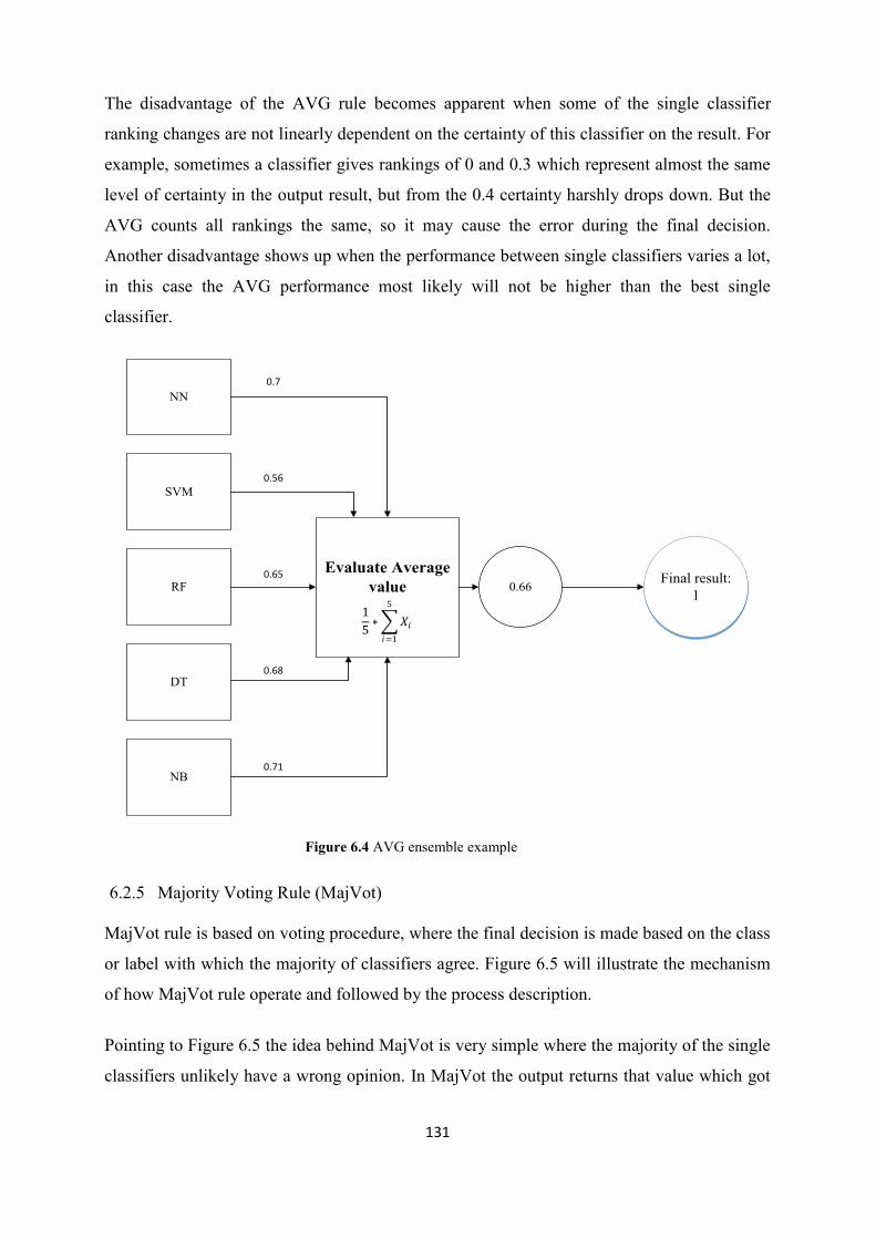
131

The disadvantage of the AVG rule becomes apparent when some of the single classifier

ranking changes are not linearly dependent on the certainty of this classifier on the result. For

example, sometimes a classifier gives rankings of 0 and 0.3 which represent almost the same

level of certainty in the output result, but from the 0.4 certainty harshly drops down. But the

AVG counts all rankings the same, so it may cause the error during the final decision.

Another disadvantage shows up when the performance between single classifiers varies a lot,

in this case the AVG performance most likely will not be higher than the best single

classifier.

NN

SVM

RF

DT

NB

Evaluate Average

value

0.7

0.56

0.65

0.68

0.71

0.66Final result:

11

5∗�𝑋𝑖

5

𝑖=1

Figure 6.4 AVG ensemble example

6.2.5 Majority Voting Rule (MajVot)

MajVot rule is based on voting procedure, where the final decision is made based on the class

or label with which the majority of classifiers agree. Figure 6.5 will illustrate the mechanism

of how MajVot rule operate and followed by the process description.

Pointing to Figure 6.5 the idea behind MajVot is very simple where the majority of the single

classifiers unlikely have a wrong opinion. In MajVot the output returns that value which got

132

the most of the classifiers votes. Obviously, with such a hierarchy, there is no need of the

threshold, only the numbers of votes given for each class are being compared, thus the final

prediction class, is that class, for which a majority of votes is given. In case of equality to tie-

in the numbers of the votes, the ensemble would classify the data point as bad loan (but in the

current case it is impossible, as there is an odd number of single classifiers).

NN

SVM

RF

DT

NB

Majority Rule

Ensemble

0.7

0.43

0.56

0.68

0.71

3>2

Quantity

estimating

Final result:

1

1

𝑁∗�𝑋𝑖

𝑁

𝑖=1

Result:

1

Result:0

Result:0

Result:

1

Result:

1

Figure 6.5 MajVot ensemble example

The MajVot avoids the first disadvantage; which AVG classifier has. MajVot is a very solid

classifier, which is simple to use and which often gives good performance. The bad efficiency

of a single classifier will not matter if all other classifiers performance is good. The Accuracy

of classifiers would matter only when number of such classifiers becomes approximately

equal to half of the number of all classifiers. However, this ensemble also has a shortcoming,

that are connected to simplifying the single classifiers output and sometimes loosing valuable

information.

133

6.2.6 Weighted Average Rule (WAVG)

WAVG rule is based on taking the average or mean value raking of all classifiers with a

weight associated to every ranking based on its performance to be chose as final ranking..

Figure 6.6 will illustrate the mechanism of how MajVot rule operate and followed by the

process description.

The WAVG ensemble is similar to AVG ensemble. The difference between them lies in the

weighting each classifier's output before finding the average value. Weighting coefficients are

evaluated according to single classifiers global Accuracy over the training set: the more

accurate classifier is on the training set, the bigger is weight coefficient assigned to this

classifier. An undeniable advantage of such development is the possibility to make more

accurate classifiers decisions more affecting the ensemble result, while less accurate

classifiers give less contribution to the final result.

However, WAVG has a very serious shortcoming, which is related to the fact that some

single classifiers tend to be over-trained, and give much better results over the training data

than over the testing data. The examples of such classifiers are NN, RF and SVM. That is

why some good classifiers may get low weights, which will have negative impact on the

WAVG result. The method how to overcome this disadvantage lies in increasing training set

until training set Accuracy of all classifiers is equally proportional to the test set Accuracy.

134

NN

SVM

RF

DT

NB

Weighted average

Ensemble

0.7

0.56

0.65

0.68

0.71

0.78 Threshold PassingFinal result:

11

𝑁∗�𝑋𝑖

𝑁

𝑖=1

∗ 𝐶𝑖

Ci – weight of a classifier

The weights are being

evaluated dependently on

the classifier`s accuracy

over the training data

Figure 6.6 WAVG ensemble example

6.2.7 Weighted Voting Rule (WVOT)

WVOT rule is based on the same idea of MajVot but each class is given a weight, the weights

of each class are combined and the decision of the final class is based on the highest value

after applying a threshold. Figure 6.7 will illustrate the mechanism of how MajVot rule

operate and followed by the process description.

WVOT is similar to MajVot ensemble. The difference between them lays in several

preparation steps before quantity estimating. The first step is rounding the single classifiers

output to the nearest integer. Weighting vector builds according to the same algorithm as in

the previous combiner WAVG. In the next step a linear combination of coefficients is done

dependently on the absolute Accuracy of each classifier on a training set. Then, the scalar

product of vector of weights is being performed and rounded vector of single classifiers

rankings. WVOT has the same disadvantage as WAVG, and it can be overcoming in the same

way.

135

NN

SVM

RF

DT

NB

Weighted Voting

Ensemble

0.7

0.43

0.49

0.68

0.71

0.65 > 0.35

Quantity

estimating

Final result:

1

1

𝑁∗�𝑋𝑖

𝑁

𝑖=1

𝐶𝑖 = 1

𝑁

𝑖=1

Rounding to

the integerWeighting

Weighting

Weighting

Weighting

Weighting

Rounding to

the intrger

Rounding to

the integer

Rounding to

the integer

Rounding to

the integer

1

0

1

0

1

0.3

0.15

0.2

0.2

0.15

Dependently on

absolute accuracy over

the training data

Figure 6.7 WVOT ensemble example


In this section results of the seven traditional combiners across seven datasets evaluated on

six performance measures are summarised and discussed (The results are evaluated by taking

the average of 50 testing sets resulting from the 10 × 5 cross-validation). All the base single

classifiers predictions is combined, their results is analysed, discussed and assumptions is

made on why these results and what they are. Tables 6.1 to 6.7 will demonstrate the results of

each combination method across all dataset on several performance measures.

136

6.3.1 Min Rule Results

According to Table 6.1, the MIN rule obviously gives good results on data sets for which

percentage of good loans is high (e.g., German, Iranian and UCSD datasets), although it's

result on the UCSD dataset is still very good. When comparing with MAX, it becomes clear

that there is 1% decrease over German dataset and 4% increase over Iranian and UCSD

dataset), the reason of this was described in previous section. On Polish dataset, results of

MIN are amongst one of the worst, when comparing to all other traditional combiners. Due to

threshold adjustment, levels of sensitivity and specificity are more or less balanced (except

for Iranian dataset, where specificity is 0).


Accuracy 0.7636 0.8662 0.8643 0.9500 0.7204 0.8246 0.8046

Sensitivity 0.9239 0.8927 0.9102 1 0.9052 0.9830 0.8576

Specificity 0.3920 0.8324 0.8087 0 0.5616 0.1906 0.7873

AUC 0.7178 0.9126 0.9130 0.5533 0.8287 0.8059 0.8828

Brier Score 0.2058 0.1153 0.1139 0.0494 0.2637 0.1466 0.1960

H-measure 0.2248 0.6355 0.6336 0.0545 0.3961 0.3837 0.4616

Table 6.1 MIN combination results

In Figure 6.8, the best results MIN provides across the Australian and Japanese datasets. For

UCSD dataset performance of MIN is also good. The worst dataset is Iranian, where the plot-

ROC curve lies almost on the diagonal. The Jordanian and the German has the same pattern

however, Jordanian is better. Very interesting is the Polish dataset ROC curve, which is not

convex for some threshold range. It is worth mentioning to describe the thresholds assigned to

each classifier for each dataset, Table 6.2 illustrates this:

Dataset German Australian Japanese Iranian Polish Jordanian UCSD

Threshold 0.326682 0.380086 0.465883 0.258415 0.236384 0.203055 0.428176

Table 6.2 MIN thresholds across all datasets

137

Figure 6.8 MIN ROC curve for all datasets

6.3.2 Max Rule Results

The MIN and MAX combiners are better to describe and analyse together, since they are two

extremes of one rule. Table 6.3 reveals that the work of these two combiners is very similar;

they both strongly depend on how good classifiers are trained. Also, as well as MIN

combiner, MAX works better on datasets with high percentage of bad loans. This could be

clearly seen on Polish dataset, comparing to MIN. Another reason of mistakes could be an

inappropriate is the choosing of threshold. For example, the MIN combiner outputs only zeros

on the Iranian dataset, whereas the threshold of MAX combiner allows it to allocate ones,

although the Accuracy rapidly decreases. However, in some cases, like with MIN on the

Iranian dataset, it is impossible to set an appropriate threshold. This is happening when one

class data prevails over the other class.

138


Accuracy 0.7532 0.8662 0.8449 0.9101 0.7679 0.8528 0.8416

Sensitivity 0.7899 0.8235 0.7638 0.9430 0.5826 0.9059 0.4713

Specificity 0.6697 0.9185 0.9458 0.2998 0.9334 0.6431 0.9626

AUC 0.7878 0.9075 0.9028 0.7401 0.8240 0.8607 0.8357

Brier Score 0.1951 0.1108 0.1641 0.0712 0.1881 0.1154 0.1247

H-measure 0.2879 0.6319 0.6137 0.2541 0.4086 0.4693 0.4011

Table 6.3 MAX combination results

According to Figure 6.9 the MAX rule has the highest is Australian and Japanese datasets, the

Jordanian comes third. MAX is good on a datasets with high amount of bad loans, so the

ROC curve for the Iranian dataset is a lot higher than that in the MIN. UCSD ROC curve is a

polyline, which means that for this dataset MAX is not very stable with respect to threshold

changings. It means that the threshold cannot be changed in order to obtain a desired

sensitivity, with a specificity value decreased very much. It is worth mentioning to describe

the thresholds assigned to each classifier for each dataset, Table 6.4 illustrates this:


Threshold 0.510207 0.598982 0.559070 0.396230 0.537883 0.578746 0.599937

Table 6.4 MAX thresholds across all datasets

139

Figure 6.9 MAX ROC curve for all datasets

6.3.3 Product Rule Results

As it has already been mentioned, the PROD is very sensitive to each input value from the

classifiers. This particular feature makes the threshold very hard to set perfectly, even the

small change in one input value, which makes no real difference, may totally change the

result of the combiners work. This can be seen in Table 6.5 results where exactly this feature

produces that same situation on the Iranian dataset as the MIN has, and makes it useless on

this particular dataset. Unlike Min and MAX combiners, the Accuracy of PROD does not

depend on the ratio of good and bad loans. The best results are shown on Australian and

Japanese datasets, datasets with the least number of features, although it is not a feature of

PROD particularly, but of all the combiners.

140


Accuracy 0.7362 0.8583 0.8597 0.9500 0.7187 0.8156 0.8030

Sensitivity 0.9828 0.9149 0.9094 1 0.9437 0.9948 0.8665

Specificity 0.1624 0.7867 0.7991 0 0.5243 0.0986 0.7822

AUC 0.7089 0.9116 0.9100 0.5384 0.8186 0.7727 0.8934

Brier Score 0.2316 0.1234 0.1225 0.0500 0.2687 0.1683 0.1862

H-measure 0.2246 0.6381 0.6332 0.0500 0.3950 0.4099 0.4727

Table 6.5 PROD combination results

Figure 6.10 shows that PROD ROC curves behave similarly as the MIN. The only difference

is that for some threshold values. UCSD ROC curve stays behind the two leaders (Australian

and Japanese datasets). This can be considered as advantage of PROD against other

classifiers. So for real-life datasets using of PROD may be justified. However, on German

and Iranian datasets PROD shows bad performance, these two dataset are the worst in terms

of AUC and ROC curve shapes. It is worth mentioning to describe the thresholds assigned to

each classifier for each dataset, Table 6.6 illustrates this:


Threshold 0.200688 0.201351 0.205318 0.599964 0.241857 0.201298 0.205830

Table 6.6 PROD thresholds across all datasets

141

Figure 6.10 PROD ROC curve for all datasets

6.3.4 Average Rule Results

Table 6.7 demonstrates that AVG is one of the best classifiers, the reason has already been

mentioned, it relies on every input value from single classifiers. Unlike the PROD, a slight

change of one value is not capable of changing the final result. Even approximately, AVG

looks like highly improved than the PROD. In Chapter 3 it was mentioned that AUC metric

could be explained as the flexibility of the classifier. This classifier shows the best flexibility

in pair with very low losses which is represented by the Brier Score. However, this is not

enough to prevent only '0' output on the Iranian dataset, which is still the only dataset that so

poorly classified by all combiners.

142


Accuracy 0.7730 0.8725 0.8648 0.9500 0.7817 0.8566 0.8639

Sensitivity 0.9014 0.8586 0.8437 1 0.7917 0.9607 0.7040

Specificity 0.4759 0.8890 0.8921 0 0.7787 0.4429 0.9158

AUC 0.7996 0.9294 0.9262 0.7770 0.8594 0.8817 0.9082

Brier Score 0.1584 0.0977 0.1005 0.0432 0.1527 0.1036 0.0999

H-measure 0.3063 0.6515 0.6468 0.2931 0.4461 0.4945 0.5160

Table 6.7AVG combination results

AVG is a very good combiner, and this fact is reflected in its ROC curves for all datasets in

Figure 6.11. AVG includes all single classifiers rankings equally, that’s why the rankings of

AVG rule are very versatile and that is why the ROC curves are round-shaped (not similar to

polylines, like plot-ROC curves of previous combiners). The leaders are the same (Australian

and Japanese datasets) with UCSD and Jordanian datasets in the third and fourth place

respectively. Even the ROC curve for Iranian dataset is not extremely low; it is close to the

ROC curve of the German dataset. Polish ROC curve is a bit jagged, which can be explained

by the small size of the Polish dataset.

143

Figure 6.11 AVG ROC curve for all datasets

6.3.5 Majority Voting Rule Results

In Table 6.8, MajVot demonstrates the best performance amongst all combiners. Although it

is not so multi-purposed as AVG, but it still has better Accuracy. This classifier shows us the

simple truth that there is no need for sophisticated analysis, when working with results of

many single classifiers. The result of the most ‘sure’ or ‘confident’ classifier is pretty enough.

Unfortunately, there is still a problem with the Iranian dataset where the most 'confident'

result would always be close to '0' on this dataset. This fact makes the most optimistic

combiner useless on the Iranian dataset.

144


Accuracy 0.7776 0.8736 0.8654 0.9500 0.7883 0.8604 0.8649

Sensitivity 0.9059 0.8642 0.8449 1 0.7989 0.9625 0.6859

Specificity 0.4859 0.8848 0.8918 0 0.7847 0.4555 0.9236

AUC 0.7548 0.9031 0.9082 0.5777 0.8578 0.8025 0.8772

Brier Score 0.1837 0.1106 0.1108 0.0471 0.1584 0.1136 0.1068

H-measure 0.2859 0.6382 0.6408 0.1089 0.4415 0.4345 0.4975

Table 6.8 MajVot Rule combination results

As it can be seen from Figure 6.12, MajVot ROC curves are always polylines, as MajVot can

take a limited number of values (0, 0.2, 0.4, 0.6, 0.8, 1). That is because the ranking of

MajVot is calculated as number of classifiers which vote that loan is bad, divided by the

whole number of classifiers. That’s why results of MajVot are not flexible with threshold

changing. While threshold is changing in (0.4, 0.6) interval, Accuracy remains the same, but

as soon as threshold exceeds 0.6, sensitivity dramatically rises, and specificity even more

dramatically falls. But for some datasets MajVot gives the best performance over all

combiners, so the final decision about which classifier to choose should be made using

additional dataset measurements. Three leaders are the same as in AVG rule; however the

ROC curve of Iranian dataset is much lower than other ROC curves.

145

Figure 6.12 MajVot ROC curve for all datasets

6.3.6 Weighted Average Rule Results

According to Table 6.9, this combiner, as a developed version of AVG combiner, takes into

consideration Accuracy of single classifiers when computing final ranking. Now classifiers

with bad Accuracy on training set have a little weight, and their influence is not enough to

change the final result to incorrect. The problem appears if highly weighted classifier makes a

mistake. Such situation may cause a mistake of all combiner. Such change instead of

increasing Accuracy decreases it. Decrease differs from 0.12% on Australian dataset, to

impressive 4.55% on Polish dataset, when compared to AVG. On the Jordanian dataset, on

the other hand, WAVG shows the best results. In general, WAVG performs well on the

datasets, where training set Accuracy correctly reflects single classifier quality, this became a

problem on a small dataset like Polish, where some classifiers on training set can show very

high Accuracy (due overtraining), but this has nothing in common with real quality of

classifier. It is worth mentioning to describe the weights or coefficients assigned to each

classifier for each dataset, Table 6.10 illustrates this:

146


Accuracy 0.7458 0.8713 0.8536 0.9497 0.7362 0.8622 0.8602

Sensitivity 0.8604 0.8789 0.9145 0.9898 0.7434 0.9327 0.7032

Specificity 0.4806 0.8611 0.7798 0.1978 0.7368 0.5842 0.9114

AUC 0.7459 0.9202 0.9091 0.7759 0.8010 0.8791 0.9011

Brier Score 0.1798 0.1021 0.1218 0.0452 0.1874 0.1014 0.1022

H-measure 0.2225 0.6356 0.6012 0.2838 0.3224 0.5064 0.5056

Table 6.9 WAVG combination results


RF 0.58 0.18 0.58 0.68 0.63 0.34 0.55

DT 0.21 0.35 0.03 0.08 0.01 0.12 0.30

NB 0.12 0.00 0.20 0.21 0.29 0.00 0.00

NN 0.09 0.28 0.19 0.00 0.07 0.17 0.07

SVM 0.00 0.19 0.00 0.03 0.00 0.38 0.08

Table 6.10 WAVG coefficients for each dataset for all classifiers

WAVG performance in terms of ROC curves is similar to AVG. Figure 6.13 shows that

Japanese dataset is slightly worse than Australian dataset. Surprisingly, the Jordanian dataset

shows solid ROC curve just after the UCSD ROC curve. The main problem of WAVG, as it

was mentioned before, is inconsistency between training set Accuracy and testing set

Accuracy, that’s why weighted coefficients may not always be optimal. This is the reason

why the most accurate classifier RF can receive lower weights than NN, which can show

even 100% Accuracy over the training set.

147

Figure 6.13 WAVG ROC curve for all datasets

6.3.7 Weighted Voting Rule Results

The results of Table 6.11 are seen to be similar to MajVot; however, in this combiner the

most effect on the results is caused by the weights. As far as the classifiers outputs are being

rounded, the uncertainty of the classifier does not cause any effect, the output could be on the

edge with the threshold value, the mistake could be minimal, but rounding has a critical

chance to change the combiner's result to wrong prediction. Thus, the possible reason is that

the mistake might become a common situation, when classifiers are uncertain about some

data. It is worth mentioning to describe the weights or coefficients assigned to each classifier

for each dataset, Table 6.12 illustrates this.

148


Accuracy 0.7725 0.8700 0.8717 0.9460 0.7742 0.8574 0.8690

Sensitivity 0.9066 0.8766 0.8806 0.9875 0.7782 0.9412 0.6924

Specificity 0.4611 0.8607 0.8618 0.1619 0.7774 0.5269 0.9269

AUC 0.6878 0.8908 0.8486 0.5723 0.7990 0.7954 0.8093

Brier Score 0.1933 0.1064 0.1154 0.0477 0.1990 0.1098 0.1145

H-measure 0.2473 0.6308 0.6113 0.1059 0.3843 0.4297 0.4809

Table 6.11 WVOT combination results


RF 0.71 0.19 0.46 0.29 0.70 0.20 0.53

DT 0.09 0.57 0.00 0.32 0.00 0.23 0.30

NB 0.00 0.00 0.22 0.26 0.08 0.00 0.00

NN 0.04 0.04 0.19 0.13 0.04 0.18 0.10

SVM 0.16 0.19 0.12 0.00 0.18 0.39 0.06

Table 6.12 WVOT coefficients for each dataset for all classifiers

Looking at Figure 6.14, WVOT ROC curves are similar to MajVot ones, and as that

classifier, WVOT ROC curves are polylines, which can be explained by the same way as

MajVot. WVOT shows good performance on Australian, Japanese and UCSD datasets,

however the ROC curve for the UCSD dataset drastically falls down on a low threshold

values. But on the high values of threshold performance of UCSD is even better than

Japanese and Australian performance.

149

Figure 6.14 WVOT ROC curve for all datasets


In this section all traditional combiners are analysed, compared between each other's and with

LR. Then, some assumptions are made for which type of datasets; combiner would show the

best performance. Firstly, the ranking table of all traditional combiners is given. It would help

to analyse, which combiner shows the best Accuracy and for which dataset.

German Australian Japanese Iranian Polish Jordanian UCSD Average ranking

MIN 4 5 4 1 6 6 6 4.57

MAX 5 5 7 4 4 5 5 5

PROD 7 6 5 1 7 7 7 5.71

AVG 2 2 3 1 2 4 3 2.43

MajVot 1 1 2 1 1 2 2 1.43

WAVG 6 3 6 2 5 1 4 3.86

WVOT 3 4 1 3 3 3 1 2.57

Table 6.13 Global rating of traditional combiners by Accuracy

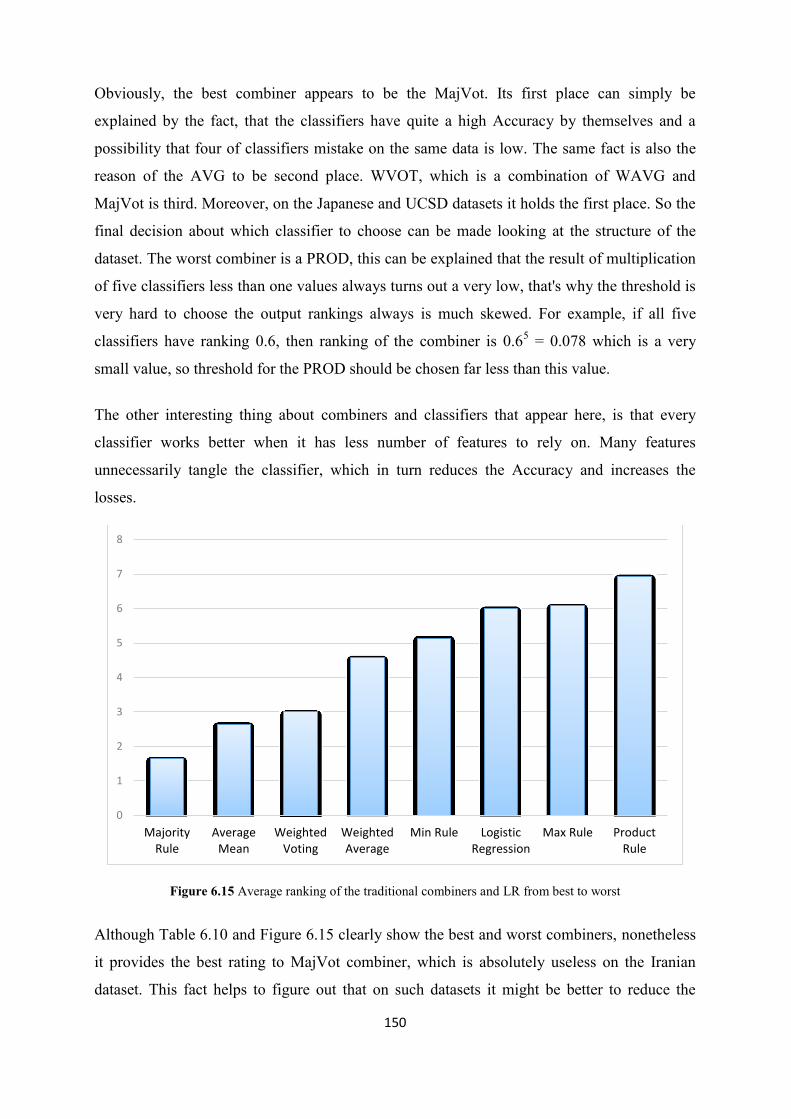
150

Obviously, the best combiner appears to be the MajVot. Its first place can simply be

explained by the fact, that the classifiers have quite a high Accuracy by themselves and a

possibility that four of classifiers mistake on the same data is low. The same fact is also the

reason of the AVG to be second place. WVOT, which is a combination of WAVG and

MajVot is third. Moreover, on the Japanese and UCSD datasets it holds the first place. So the

final decision about which classifier to choose can be made looking at the structure of the

dataset. The worst combiner is a PROD, this can be explained that the result of multiplication

of five classifiers less than one values always turns out a very low, that's why the threshold is

very hard to choose the output rankings always is much skewed. For example, if all five

classifiers have ranking 0.6, then ranking of the combiner is 0.65 = 0.078 which is a very

small value, so threshold for the PROD should be chosen far less than this value.

The other interesting thing about combiners and classifiers that appear here, is that every

classifier works better when it has less number of features to rely on. Many features

unnecessarily tangle the classifier, which in turn reduces the Accuracy and increases the

losses.

Figure 6.15 Average ranking of the traditional combiners and LR from best to worst

Although Table 6.10 and Figure 6.15 clearly show the best and worst combiners, nonetheless

it provides the best rating to MajVot combiner, which is absolutely useless on the Iranian

dataset. This fact helps to figure out that on such datasets it might be better to reduce the

0

1

2

3

4

5

6

7

8

MajorityRule

AverageMean

WeightedVoting

WeightedAverage

Min Rule LogisticRegression

Max Rule ProductRule

151

Accuracy but be able to find the '1's amongst the ocean of '0's and reduce the losses, as far as

all the combiners are being considered for being used in credit-scoring. Finally, the traditional

combiners could be used to improve the work of single classifiers, but these could not be used

on every dataset with the same productivity, and should be chosen dependently on each

dataset. Logistic regression, a benchmark classifier, holds the sixth position, which

demonstrates that using novel pre-processing techniques and strong classifiers helps to beat

LR even if very simple combiners were used.

One more dataset that requires some extra analysis is the UCSD dataset. This dataset clearly

shows, as in Table 6.14, that most of combiners are absolutely capable of giving results better

than Logistic Regression. There are two combiners that are very worse than LR which are the

MIN and PROD, and both these cases can be easily explained by the fact that the UCSD

dataset is a large real-world dataset which is highly imbalanced where it has around 75% of

good loans, and MIN and PROD in general have bad performance for such datasets. MAX

gives almost the same performance as Logistic Regression, and all other combiners are better

up to +2.73% for WVOT. As this dataset is a large real-world dataset, this fact is remarkable

and worth mentioning.

Table 6.14 provides the Accuracy of LR which shows how the Accuracy of traditional

combiners varies from them. The value is positive if combiner's Accuracy is better, and

negative otherwise. Subsequently, the table is illustrated in Figure 6.16.


Logistic Regression 0.7597 0.8641 0.8626 0.9239 0.7246 0.8240 0.8417

MIN 0.0039 0.0021 0.0017 0.0261 -0.0042 0.0006 -0.0371

MAX -0.0065 0.0021 -0.0177 -0.0138 0.0433 0.0288 -0.0001

PROD -0.0235 -0.0058 -0.0029 0.0261 -0.0059 -0.0084 -0.0387

AVG 0.0133 0.0084 0.0022 0.0261 0.0571 0.0326 0.0220

MajVot 0.0179 0.0095 0.0028 0.0261 0.0637 0.0364 0.0232

WAVG -0.0139 0.0072 -0.0090 0.0198 0.0116 0.0382 0.0185

WVOT 0.0128 0.0059 0.0091 0.0221 0.0496 0.0334 0.0273

Table 6.14 Difference with Logistic Regression

152

Figure 6.16 Accuracy difference with Logistic Regression

In fact, the table and graph only approve the conclusions made after the ranking table built.

The only thing that should be mentioned once more is the Iranian dataset. Although every

combiner is better on this dataset, it should not be forgotten, that most of combiners outputs

are good loans only. Thus, the superiority of such combiners is very doubtful.

6.5 Summary

The results obtained clearly show that most traditional combiners concede the best of

classifiers (RF) for all datasets. Of course, RF stays the best, but actually it is not a single

classifier but a homogenous combiner of DT.

However, all traditional combiners could be categorized into two groups. The first one, which

gives comparatively good results, that includes the MajVot, AVG and WVOT. These three

classifiers compared to LR shows better results in the main measures (e.g., Accuracy, AUC)

for all datasets without exception. The second group consists of MIN, MAX, PROD and

WAVG, these shows the worse classifiers, which are worse than LR for some datasets.

Advantages of traditional combiners from the first group are:

Simplicity and intuitiveness of the mathematical model of the combiner.

High stable results over all datasets.

-6

-4

-2

0

2

4

6

8

Min Rule Max Rule Product

Rule

Average

Mean

Majority

Rule

Weighted

Average

Weighted

Voting

Accuracy difference

German Aust Japanese Iranian Polish Jordanian UCSD

153

The second advantage should be explained: even though for some datasets single classifiers

can have advantage over traditional combiners and other single classifiers, for other datasets

for some reason results of single classifiers can become significantly worse than other

classifiers results. The example is DT in Polish dataset where it shows Accuracy even better

than Accuracy of RF, but for German dataset it shows the worst Accuracy amongst single

classifiers. Traditional combiners from the first group, on the other hand, show stable results

without significant drops and rises for all datasets.

Therefore, traditional combiners from the first group could be used in real-life applications if

they know that input data is varying a lot (input datasets have highly different number of

features, percentage of bad loans, number of outliers and noise etc.) so if traditional

combiners were used, it can be assured that the results would be good enough for all type of

datasets. The selecting of specific combiner between the first group is up to the a priori

knowledge about structure and parameters of a majority of input datasets.

On the other hand, the general performance of the traditional combiners has proven

insufficient as the Accuracy of the best of traditional combiner concedes the Accuracy of

RFs. As a result, in the next chapter an analysis to such complex combiners such as D-ENS

and classifier ConsA is undertaken and evaluation of their performance in comparison to the

performance of all single and hybrid classifiers and traditional combiners that have been

investigated in this and previous chapters.

154

CHAPTER 7

HYBRID ENSEMBLE CREDIT-SCORING MODEL USING

CLASSIFIER CONSENSUS AGGREGATION APPROACH

7.1 Introduction

In Chapter 5, it has been demonstrated that single classifiers performance are increased when

applying such pre-training data-selection algorithms as filtering and feature selection were

analysed. In Chapter 6 simple heterogeneous combiners in the hope that they show better

results than the best of single classifiers were considered. Unfortunately, the results of

traditional combiners showed drawbacks of traditional approaches to create ensembles of

single classifiers. In this Chapter, 2 ensemble algorithms, which are inherently different, were

proposed in the hope of showing high and stable results over all datasets.

In reference to Table 2.2, amongst 37 studies that has been investigated, it can be noticed that

only few number of studies focused on using selective ensembles and different classifiers

combination methods. For this reason this chapter will focus on developing different

combination approached in the hope of increasing the model performance.

Multiple classifiers systems or classifiers ensembles can be combined in 2 ways, either fusion

of the classifiers or dynamic classifier(s) selection (Woods et al., 1997; Ko et al., 2008; Xiao

et al., 2012). Classifier fusion methods take all classifiers rankings and combine them in one

classifier which also can be called static ensemble. On the other hand dynamic selection can

be either a selection of one best classifier or best group of classifiers from the pool of

classifiers that can classify each test sample; these two types of selection are called dynamic

classifier selection or D-ENS selection (Xiao et al., 2012). According to Ko et al. (2008) the

advantage of D-ENS over classifier selection is the distribution of the risk of over-

generalisation by choosing a group of classifiers instead of one for a test point. Therefore, D-

ENS selection approach is adopted in this work.

In this chapter new ensemble algorithms which belong to dynamic and static combination

approaches is investigated. The first algorithm is called the D-ENS classifier; its idea is

155

inspired from Xiao (2012) which is that in different areas of input N-dimensional space

(where N is number of features in dataset) different classifiers can be amongst the leaders in

terms of classification Accuracy. So for each point local Accuracy of each single classifier

amongst the training set is calculated, and evaluate weighting coefficients 𝑤𝑖 proportional to

these values. The ranking of the D-ENS classifier would be a linear combination of single

classifiers rankings with the weights‍𝑤‍𝑖.

The second approach is called the classifiers ConsA (DeGroot, 1974; Berger, 1981Shaban et

al., 2002) it simulates a behaviour and team-communication process of real experts group, so

that each of single experts can modify its own opinion accordingly to opinions of other

experts in the group. The final ranking of ConsA classifier is calculated as a common group

decision after equilibrium is reached and opinions do not change anymore. Besides, the D-

ENS and ConsA algorithms are connected with the approaches described in the fourth chapter

in the hope than if single classifiers shows better results, complex combiners will increase

their Accuracy even more.

7.2 The Proposed Approaches

In this section, models of modern and efficient combiners: D-ENS classifiers and classifiers

ConsA are considered. Both these models are complex and that is why they show different

behaviour in different points of input space (unlike classical combiners, which depends only

on single classifiers rankings, and evaluate final ranking using one fixed equation without

dynamic additional parameters).

7.2.1 The Dynamic Ensemble Approach

The proposed model of D-ENS classifiers approach is shown in Figure 7.1. In this model, two

pre-training phases were used before actually starting single classifiers training. Parameters of

single classifiers, including feature selection importance threshold and filtering thresholds

𝑇𝑟0‍and 𝑇𝑟1 are remaining the same as in Chapter 5.

156

Input data

Dynamic ensemble based

on local accuracy

Training data Testing data

Delete unnecessary

features

Data Filtering

MARS feature

selection

Random

Forest

Naive

Bayes

Decision

Tree

Neural

NetworkSVM

Ensemble Decision

Dynamic ensemble

algorithm

Dynamic ensemble

rankings

Figure 7.1 The process of the D-ENS Approach

The workflow of the dynamic classifiers ensemble can be summarised in the following steps:

Divide input data into training and testing set.

Evaluate MARS model onto training data to obtain list of selected features.

Build proximity graph and filter training data (the goal of filtering is removing outliers

and highly noisy data points)

Train five classifiers and obtain classifiers rankings for testing set queries.

Perform D-ENS classifiers algorithm to merge single classifiers rankings into one.

The details of the D-ENS approach are discussed in Section 7.3.

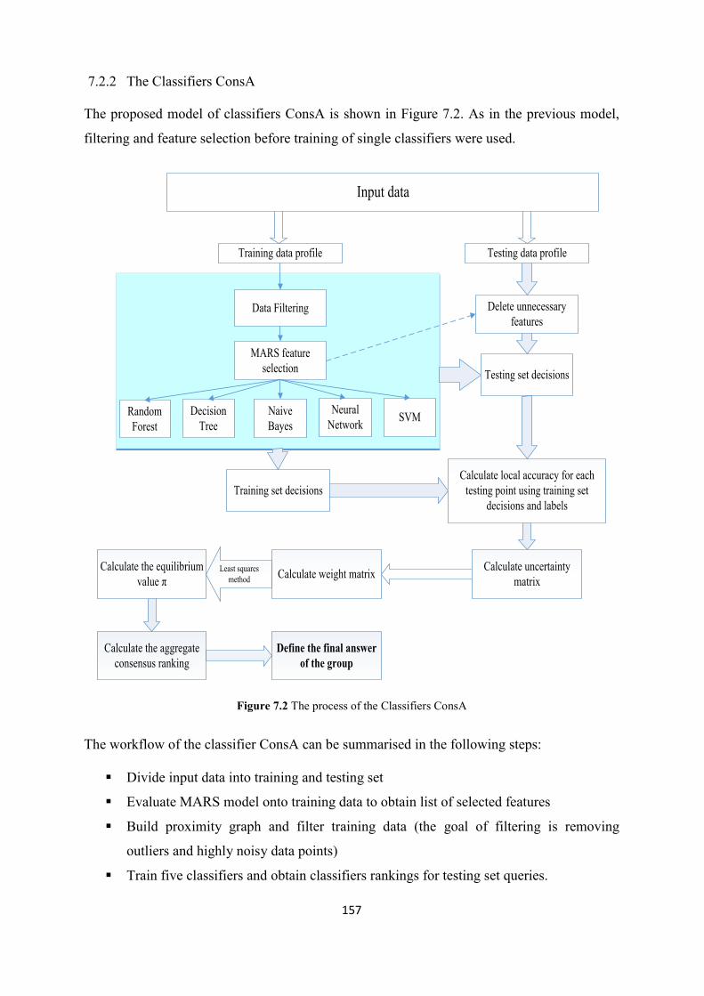
157

7.2.2 The Classifiers ConsA

The proposed model of classifiers ConsA is shown in Figure 7.2. As in the previous model,

filtering and feature selection before training of single classifiers were used.

Data Filtering

MARS feature

selection

Random

Forest

Naive

Bayes

Decision

Tree

Training data profile Testing data profile

Neural

NetworkSVM

Calculate uncertainty

matrix

Testing set decisions

Calculate weight matrixCalculate the equilibrium

value πLeast squares

method

Calculate the aggregate

consensus ranking

Define the final answer

of the group

Input data

Training set decisions

Calculate local accuracy for each

testing point using training set

decisions and labels

Delete unnecessary

features

Figure 7.2 The process of the Classifiers ConsA

The workflow of the classifier ConsA can be summarised in the following steps:

Divide input data into training and testing set

Evaluate MARS model onto training data to obtain list of selected features

Build proximity graph and filter training data (the goal of filtering is removing

outliers and highly noisy data points)

Train five classifiers and obtain classifiers rankings for testing set queries.

158

For each testing set query:

- Calculate local Accuracy for each single classifier using training set queries

and actual labels for these queries

- Calculate uncertainty matrix of group of classifiers.

- Calculate weight matrix.

- Calculate equilibrium value (group vector of rankings using least square

method not iterations method as in DeGroot (1974).

- Calculate the aggregate ConsA ranking.

- Using default value of threshold, calculate the final answer (prediction) of the

group.

- The details of the classifiers ConsA is discussed in Section 7.4.

7.3 D-ENS Approach: Description of the Algorithm

In this section the theory which lies behind dynamic classifier ensemble model is

demonstrated in addition to the explanation of the approach which is developed and tested in

this work. D-ENS is a fusion model, which is based on the idea to combine rankings of single

classifiers taking into account their local accuracies. Local Accuracy is estimated by the

Accuracy of each classifier in the local region of the feature space surrounding an unknown

test point (Woods et al., 1997; Oza et al., 2005). To evaluate local Accuracy Xiao et al.

(2012) proposed to put forward two calculation methods: overall local Accuracy (OLA) and

local class Accuracy (LCA). The Accuracy of D-ENS strictly depends on the correctness of

the local Accuracy estimate, so it is important to choose right local Accuracy evaluation range

and choose whether to use overall local Accuracy or simple local class Accuracy. To avoid

the problem of choosing these parameters, it is proposed to modify the LCA evaluation

method so that it can be taken into consideration the Accuracy in the all points, but with the

weight inverse proportional to the distance from the target point. This approach will

overcome heterogeneity in the input data, so that for some points the number of local

neighbours can be too small, and that's why local Accuracy is not precise.

D-ENS is a combiner which outperforms best classifiers results over the majority of data sets

(Woods et al., 1997). Initially, Xiao et al. (2012) investigated the dynamic classifier selection

method, which for each testing set point returns as the output ranking of the best classifier in

159

that point (in terms of local Accuracy). As an inspiration from their method, the proposed

method will take into consideration other classifiers with less local Accuracy (however, their

impact is less than impact of classifier with the best local Accuracy). In other words in the

proposed approach the final output is linear combination of single classifiers outputs, with

weights proportional to local Accuracy for each testing set point rather than taking the final

output as the ranking of the most accurate classifier. This allows to build more flexible and

robust ensemble, as even the best classifier could be sometimes wrong.

Before applying the ensemble combiner, all single combiners (RF, DT, NB, NN and SVM)

are trained and evaluate their predictions over training and testing sets. To combine the

decisions of these five classifiers the local Accuracy is evaluated for each entry 𝑥∗ from a

testing set. In Xiao et al. (2012) it is proposed to choose non-negative distance 𝑑 as a local

Accuracy area and evaluate Accuracy over all entries from training set that are located at a

distance from 𝑥∗ less than 𝑑. As an enhancement, it is proposed to evaluate not a simple mean

value, but weighted average for all points from training set with weights are inversely

proportional to the distance from training test entries to 𝑥∗ In other words, lets have a training

set entries 𝑥𝑖 with target labels 𝑝𝑖, and classifier's predictions over training set 𝑝�̃�, where

𝑖 = 1. . . 𝑁. Local Accuracy is evaluated as:

𝐿(𝑥∗) = ∑ ‍𝑁𝑖=1 𝑤𝑖|𝑝𝑖 − 𝑝�̃�|, ∑ ‍𝑁𝑖=1 𝑤𝑖 = 1 (7.1)

and‍𝑤𝑖 is inversely proportional to distance from 𝑥∗ to 𝑥𝑖.

Conditional local accuracies are evaluated as:

𝐿(𝑥∗, 0) = ∑ ‍𝑝𝑖=0𝑤𝑖|𝑝𝑖 − 𝑝�̃�|, ∑ ‍𝑝𝑖=0

𝑤𝑖 = 1 (7.2)

𝐿(𝑥∗, 1) = ∑ ‍𝑝𝑖=1𝑤𝑖|𝑝𝑖 − 𝑝�̃�|, ∑ ‍𝑝𝑖=1

𝑤𝑖 = 1 (7.3)

For clarity on how local Accuracy for a test point is calculated, Figure 7.5 illustrates an

example on the local Accuracy algorithm workflow for a small training and testing sets.

160

Figure 7.3 Local Accuracy evaluation example

Let’s have a training set consists of 4 points with their accuracies in each shown in the Figure

7.3 (Accuracies = [0.2,0.6,0.4,0.1]). Standard Accuracy over training set is average of these

4 numbers, so‍Accuracy =0.2+0.6+0.4+0.1

4= 0.3250. The Local Accuracy is calculated in the

test point 𝑥∗ and located in the centre; is calculated as follows:

- Determine vector of distances from this point to all points of the set, which is 𝐷 =

[0.707,1.41,2.24,2.83].

- Perform such operations over D:

𝐷 = 𝑚𝑎𝑥(𝐷) − 𝐷 → 𝐷 = [2.12,1.41,0.59,0]

‍‍‍‍‍‍𝐷 = 𝐷/𝑠𝑢𝑚(𝐷) → 𝐷 = [0.5139,0.3426,0.1435,0]

- To evaluate local Accuracy, evaluate 𝐿𝑎 = 𝐴 ⋅ 𝐷 = 0.3657

The aim of evaluating conditional local accuracies is to determine how good each classifier

can classify good and bad loans near point 𝑥∗ As some datasets used int this work are

imbalanced, cost of bad loan misclassifying is not equal to cost of good loans misclassifying.

After evaluating local accuracies for all entries from the testing set, evaluation of an

algorithm were processed.

161

Let us enumerate local classifiers as:

- RF

- DT

- NB

- NN

- SVM

Now 𝑝𝑖 means ranking, and 𝑈𝑖 – uncertainty value, 𝐿𝑖(𝑥∗), 𝐿𝑖(𝑥∗, 0), 𝐿𝑖(𝑥∗, 1) – absolute and

conditional local accuracies of i-th single classifier. The uncertainty of each classifier using

the equation 𝑈𝑖 = −𝑝𝑖 ⋅ log2(𝑝𝑖) was evaluated. Each ranking coefficient 𝑊𝑖 on (1 − 𝑈𝑖 were

multiplied. The idea behind it is to give lower coefficients to the classifiers with higher

uncertainty value. That's why classifier's local coefficient were evaluated as

𝑊𝑖 = (

𝐿𝑖(𝑥∗, 0) ∗ (1 − 𝑈𝑖), 0 < 𝑝𝑐𝑙 ≤ 𝑎𝑙 ,

𝐿𝑖(𝑥∗) ∗ (1 − 𝑈𝑖), 𝑎𝑙 < 𝑝𝑐𝑙 ≤ 𝑎ℎ,𝐿𝑖(𝑥∗, 1) ∗ (1 − 𝑈𝑖) 𝑎ℎ < 𝑝𝑐𝑙 < 1,

‍𝑖 ∈ {1. .5}. (7.4)

Parameters 𝑎𝑙 and 𝑎ℎ are selected for reasons of maximise the training set Accuracy of D-

ENS. After this vector 𝑊 = (𝑊1,𝑊2,𝑊3,𝑊4,𝑊5) is normalised:

𝑊𝑛𝑒𝑤 = 𝑊/∑ ‍5𝑖=1 𝑊𝑖. (7.5)

Next point is to evaluate weighted average of classifier's rankings with weights equal to 𝑊. In

other words, the final ranking of D-ENS classifier is evaluated as

𝑃∗(𝑥∗) = ∑ ‍5𝑖=1 𝑊𝑛𝑒𝑤(𝑖) ⋅ 𝑝𝑖, (7.6)

where 𝑝𝑖, 𝑖 ∈ {1. .5} are single classifier predictions.

D-ENS pseudo-code

Train single classifiers (RF, DT, NB, NN and SVM) over the training set and the following is

done:

- Evaluate single classifiers predictions of training set entries and testing set entries

For each entry 𝑥∗ from a testing set

162

- Evaluate local Accuracy of each classifier in the point 𝑥∗ using equations

(7.1), (7.2) and (7.3).

- Evaluate classifier's local coefficient according to equation (7.4)

- Normalise classifier's local coefficient according to equation (7.5)

- Evaluate prediction value of D-ENS 𝑃∗(𝑥∗) according to equation (7.6).

End for

The following example displays the dynamic classifiers ensemble approach workflow for a

single testing set point.

- For point x∗ from test set the local accuracies for five classifiers were evaluated,

results are:

- For RF 𝐿1(𝑥∗) = 0.8, 𝐿1(𝑥∗, 0) = 0.5, ‍𝐿1(𝑥∗, 1) = 1.0, 𝑝1 = 0.9

- For DT 𝐿2(𝑥∗) = 0.8, 𝐿2(𝑥∗, 0) = 0.9, ‍𝐿2(𝑥∗, 1) = 0.7, 𝑝2 = 0.6

- For NB 𝐿3(𝑥∗) = 0.7, 𝐿3(𝑥∗, 0) = 0.65, 𝐿3(𝑥∗, 1) = 0.8, 𝑝3 = 1

- For NN 𝐿4(𝑥∗) = 0.65, 𝐿4(𝑥∗, 0) = 0.75, 𝐿4(𝑥∗, 1) = 0.6, 𝑝4 = 0.1

- For SVM 𝐿5(𝑥∗) = 0.6, 𝐿5(𝑥∗, 0) = 0.8, 𝐿5(𝑥∗, 1) = 0.4, 𝑝5 = 0.5

Suppose‍𝑎𝑙 = 0.25, 𝑎ℎ = 0.75. As a first step, the uncertainties are calculated as follows:

𝑈1 = −𝑝1 ⋅ log2(𝑝1) = 0.136803, 𝑈2 = −𝑝2 ⋅ log2(𝑝2) = 0.442179, 𝑈3 = −𝑝3 ⋅

log2(𝑝3) = 0, 𝑈4 = −𝑝4 ⋅ log2(𝑝4) = 0.136803, 𝑈5 = −𝑝5 ⋅ log2(𝑝6) = 0.5,

Next step the classifier's local coefficients were calculated:

- As 𝑝1 > 𝑎ℎ, calculate 𝑊1 as 𝐿1(𝑥∗, 1)(1 − 𝑈1) = 0.863197

- As 𝑎𝑙 < 𝑝2 < 𝑎ℎ, calculate 𝑊2 as 𝐿2(𝑥∗)(1 − 𝑈2) = 0.446257

- As 𝑝3 > 𝑎ℎ, calculate 𝑊3 as 𝐿3(𝑥∗, 1)(1 − 𝑈3) = 0.8

- As 𝑝4 > 𝑎𝑙, calculate 𝑊4 as 𝐿4(𝑥∗, 0)(1 − 𝑈4) = 0.500855

- As 𝑎𝑙 < 𝑝5 < 𝑎ℎ, calculate 𝑊5 as 𝐿5(𝑥∗, 0)(1 − 𝑈5) = 0.446257

Then vector 𝑊𝑛𝑒𝑤 according to the equation (7.5) is normalised. Then

𝑊𝑛𝑒𝑤 = (0.282407, 0.145999, 0.261732, 0.163862, 0.145999)

Final ranking is as follows:

163

0.9 × 0.282407 + 0.6 × 0.145999 + 1 × 0.261732 + 0.1 × 0.163862 + 0.5 ×

0.145999 = 0.692884. Prediction of ensemble is ‘1’.

7.4 Classifiers Consensus Approach: Description of the Algorithm

In this section theory which lies behind ConsA model is demonstrated, along with its process

as well as the improvements which were made to adjunct ConsA model to our data. The basic

idea behind classifier decisions combination is that, when classifiers make a decision, one

should not rely only on a single classifier decision, but, rather, require classifiers to

participate in the decision-making process by combining or fusing their individual opinions or

decisions. Therefore, the core problem that needs to be addressed when combining different

classifiers is resolving conflicts between them. In other words, the problem is how to combine

the results of different classifiers to obtain better results (Chitroub, 2010; Xu et al., 1992). In

this section, a new combination method is introduced in the field of credit-scoring based on

classifier Consensus, where those in the ensemble interact in a cooperative manner in order to

reach an agreement on the final decision for each data sample.

Tan (1993) emphasized that agents working in partnership can significantly outperform those

working independently. The idea of the ConsA is not new as it has been investigated in many

studies in different fields, such as statistics, remote sensing, geography, classification, web

information retrieval and multi-sensory data (Tan, 1993; DeGroot, 1974; Benediktsson &

Swain, 1992; Shaban et al., 2002; Basir & Shen, 1993). In this context, the general strategies

adopted are those of DeGroot (1974), Berger (1981) and Shaban et al. (2002), who proposed

a framework that provides a comprehensive and practical set of guidelines on the

underpinning constructs of ConsA theory where interactions between classifiers are modelled

when an agreement between them is needed. It is believed that their strategies can be useful

when adopted for the credit-scoring domain.

ConsA is a modern combiner, which is based on the approach to consider single classifiers as

a collaborative society of agents that communicate their estimates of the input entries. After

some time passed, they reach a consensus with respect to the best decision possible. By

combining decisions made by different agents, more effective decision-making can be

achieved. There is a shortcoming of papers analysing performance of ConsA (e.g., DeGroot,

1974; Berger, 1981; Shaban et al., 2002). So the task in this work become useful as the only

one which compares ConsA performance with the performance of the wide list of other

164

classifiers and combiners, and do this comparison over seven different datasets, amongst

which there is real-life dataset.

ConsA differs from other classifier fusion techniques, as this method uses relationships

between single classifiers, and it models a process similar to the process of decision making

into the group of real experts. So this method is used in hope that this approach will allow us

to build very good and stable classifier.

Practically, ConsA mimics the team-communication processes of a real group of experts, so

that each individual expert can modify its own opinion according to the opinions of other

experts in the group. The final ranking of ConsA classifier is calculated as a common group

decision after equilibrium is reached. When opinions are no longer changing, and in order to

reach a consensus between classifiers on each input decision, a set of steps have to be

processed. These are discussed in the following sub-sections.

7.4.1 Calculating Classifiers Rankings and Build a Decision Profiles

Consider a group of N classifiers or agents, indexed by the a set 𝐴 = 𝐴1, 𝐴2, … , 𝐴𝑁. When

receiving a an input sample 𝑞, 𝐴𝑖 chooses an answer from a set of possible answers Γ =

(𝛾1, . . . , 𝛾𝑚). For each classifier or agent consider an estimate function 𝑅𝑖, which associates a

nonnegative number for every possible answer from Γ. The result of the estimate function 𝑅𝑖

is a value in the range of [0, 1] which shows the desirability of the corresponding answer.

Prediction of the classifier may be found after finding 𝑅𝑖 and applying a threshold to it.

∑ ‍𝑚𝑘=1 𝑅𝑖(𝛾𝑘) = 1‍∀𝑖 ∈ {1. . 𝑁} (7.7)

After calculating each classifier ranking, the decision profile can be represented in matrix

form as:

𝐷𝑃 =

[ 𝑅1(𝑒1) 𝑅1(𝑒2)‍ 𝑅1(𝑒3) … 𝑅1(𝑒𝑛)

𝑅2(𝑒1) 𝑅2(𝑒2) 𝑅2(𝑒3) … 𝑅2(𝑒𝑛)

𝑅3(𝑒1) 𝑅3(𝑒2) 𝑅3(𝑒3) … 𝑅3(𝑒𝑛)

𝑅4(𝑒1) 𝑅4(𝑒2) 𝑅4(𝑒3) … 𝑅4(𝑒𝑛)

𝑅5(𝑒1) 𝑅5(𝑒2) 𝑅5(𝑒3) … 𝑅5(𝑒𝑛)]

(7.8)

where n is the number of queries in the training/testing set, ei is the i-th input query and Rj

(ei); j ∈1..5 is the j-th classifier ranking for the i-th input query. So, to evaluate the uncertainty

between classifiers it is needed to process n columns of matrix DP for testing the set, input by

165

input. Therefore, the objective here is to evaluate the common group ranking 𝑅𝐺: Γ → [0,1] to

aggregate the expected rankings for all classifiers. Let Γ𝑗 be a vector of outputs of j-th

classifer: Γ𝑗 = 𝑅𝑗(Γ).

7.4.2 Calculating the Classifiers Uncertainty

After building the decision profile for the classifier rankings, the next stage is about finding a

function by which each classifier’s uncertainty can be computed. The task here is to assign

more weight to classifiers that are less uncertain about their decision, and vice versa.

However, the weighting should reflect the contrast in classifiers' decisions. During this stage,

uncertainty is divided into two types:

- Local Uncertainty.

- Global Uncertainty.

Here local uncertainty is related to the quality of the classifier's own decision in terms how

the classifier is confident about its decision, whereas global uncertainty denotes how much

the classifiers are confident about their decisions after knowing each other decisions this

emerges as the result of collaboration between classifiers taking place in the form of decision

profile exchange. At this stage a classifier is able to review its uncertainty level and modify it

given its decision as well as the decisions of others. This shows how a classifier is able to

improve its decision when other classifiers’ decisions become available.

The uncertainty matrix U can be presented as follows:

𝑈 =

[ 𝑈11 𝑈12‍ 𝑈13 … 𝑈1𝑁‍𝑈21 𝑈22 𝑈23 … 𝑈2𝑁𝑈31 𝑈32 𝑈33 … 𝑈3𝑁𝑈41 𝑈42 𝑈43 … 𝑈4𝑁𝑈51 𝑈52 𝑈53 … 𝑈5𝑁 ]

(7.9)

where Uii; i ∈1…5 is the local uncertainty of the i-th classifier, and Uij, I, j∈1…5; i ≠ j is the

global uncertainty of the i-th classifier, when it knows the ranking or the decision of the j-the

classifier. To evaluate the classifiers uncertainties, consider 𝑅𝑖(𝛾𝑘) is i-th agent ranking or

decision of answer 𝛾𝑘, and 𝑅𝑖(𝛾𝑘|Γ𝑗) is i-th agent ranking or decision of answer 𝛾𝑘 if it knows

the ranking or the decision of vector of j-th agent. Matrix U can be evaluated via the

following equations:

166

𝑈𝑖𝑖 = −∑ ‍𝑀𝑘=1 𝑅𝑖(𝛾𝑘)log𝑀(𝑅𝑖(𝛾𝑘)) (7.10)

𝑈𝑖𝑗 = −∑ ‍𝑀𝑘=1 𝑅𝑖(𝛾𝑘|Γ𝑗)log𝑀(𝑅𝑖(𝛾𝑘|Γ𝑗)) (7.11)

In equation (7.10), 𝑈𝑖𝑖 is local uncertainty of i-th classifier, and in equation (7.11), 𝑈𝑖𝑗 is

global uncertainty of i-th classifier, knowing the ranking of j-th classifier. Equations (7.10)

and (7.11) are applied knowing that equation (7.7) is fulfilled, as well as the following

equation:

∑ ‍𝑚𝑘=1 𝑅𝑖(𝛾𝑘|Γ𝑗) = 1‍∀𝑖 ∈ {1. . 𝑁} (7.12)

In the case of two possible answers: ‘0’ and ‘1’ which means 𝑀 = 2, and equations (7.7) and

(7.12) are converted into:

𝑅𝑖(0) + 𝑅𝑖(1) = 1, 𝑅𝑖(0|Γ𝑗) + 𝑅𝑖(1|Γ𝑗) = 1 (7.13)

where 𝑅𝑖(1) is i-th agent ranking of answer ‘1’ and 𝑅𝑖(0) is i-th agent ranking of answer ‘0’.

Denote 𝑅𝑖 = 𝑅𝑖(1) and 𝑅𝑖(Γ𝑗) = 𝑅𝑖(1|Γ𝑗). Then 𝑅𝑖(0) = 1 − 𝑅𝑖, and 𝑅𝑖(0|Γ𝑗) = 1 − 𝑅𝑖(Γ𝑗) .

Thus, equations (10), (11) are converted into:

𝑈𝑖𝑖 = −𝑅𝑖log2(𝑅𝑖) − (1 − 𝑅𝑖)log2(1 − 𝑅𝑖) (7.14)

𝑈𝑖𝑗 = −𝑅𝑖(Γ𝑗)log2(𝑅𝑖(Γ𝑗)) − (1 − 𝑅𝑖(Γ𝑗))log2(1 − 𝑅𝑖(Γ𝑗)) (7.15)

It is worth mentioning that the reason the uncertainties in the above two equations are

evaluated using a logarithm with base 2 is that this can be demonstrated by plotting equation

(7.15) where Uii is a function of parameter Ri. From the plot in Figure 7.4, it is clear that, if

the value of the classifier’s ranking is close to the edges of the [0,1] interval, uncertainty is

near zero (the classifier is certain about its decision). On the other hand, if the ranking is close

to the 0.5 point, uncertainty is close to the maximal value, which is one.

167

Figure 7.4 Uncertainty value 𝑼𝒊𝒊 as a function of the parameter 𝑹𝒊

In the current situation it is straight forward to calculate the local uncertainties, but when it

comes to global uncertainty there is no information available about the rankings of each

agent. In (DeGroot, 1974; Berger, 1981; Shaban et al., 2002) they investigated convergence

conditions and existing of the optimal single decision of the group. To evaluate ConsA

rankings, uncertainty approach was proposed. But as no information is available on the global

rankings, a solution is proposed which can estimate these global rankings. As the global

ranking of classifier 𝑖 with respect to classifier 𝑗 in the testing point 𝑥∗ a linear combinations

of i-th and j-th classifer with thee weights proportional to local accuracies of these classifiers

in this point were taken.

If 𝑅𝑖(Γ𝑗) values are not avaliable and to estimate them, local Accuracy of each classifier at a

given point are calculated using Algorithm (7.1)

Algorithm (7.1)

Calculate‍di = Ri − 0.5, dj = Ri − 0.5

- If 𝑑𝑖 > 0 and 𝑑𝑗 > 0 𝑑∗ = (𝑑𝑖 + 𝑑𝑗) ∗ 𝑘1

- If 𝑑𝑖 < 0 and 𝑑𝑗 < 0 𝑑∗ = (𝑑𝑖 + 𝑑𝑗) ∗ 𝑘2

168

In steps 2 and 3, when k1 and k2 are greater than 0.5, the effect of i-th classifier certainty

increasing due to similar opinion of j-th classifier. For example, if Ri = 0.6, Rj = 0.7 and

k = 1, then d∗ = (0.2 + 0.1) ∗ 1 = 0.3, and conditional ranking according to equation 16 is

Ri(Γj) = 0.3 + 0.5 = 0.8. The logic behind it is that if two experts simultaneously

considering a loan as ‘good’, after communication their certainty in that decision will increase

(thus, ranking will decrease). On the other hand, if two experts simultaneously considering a

loan as ‘bad’, after communication their certainty, the decision will increase (thus, ranking is

increased)

- If 𝑑𝑖 and 𝑑𝑗 have opposite signs, then 𝑑∗ = (𝑑𝑖 + 𝑑𝑗) ∗ 𝑘3

- 𝑅𝑖(𝛤𝑗) = 𝑑∗ + 0.5.

Evaluate Uij according to equation (7.13)

Update‍𝑈𝑖𝑗 = 𝑘4 ⋅ 𝑈𝑖𝑗/(𝐿𝐴𝑖(𝑞, 𝑛𝑛) − 𝑘5), where 𝐿𝐴𝑖(𝑞, 𝑛𝑛) is local Accuracy of i-th

classifier upon entry query 𝑞, using i-th classifier answer error upon exactly k-neighbour

queries from training set. In the current implementation, the parameter k = 4. Parameters

k1. . . k5 are chosen using Gradient Descent with the objective function, global Accuracy over

the training set. For each iteration these parameters were evaluated separately.

The sense behind 7-th step is to take into consideration local Accuracy of classifier, so the

classifier with low local Accuracy is more uncertain about its decision (as local Accuracy is

in the denominator). Coefficient 𝑘5 is a normalising coefficient which picks lower than the

lowest local Accuracy for i-th classifier so denominator stays positive.

7.4.3 Calculating the Classifiers Weights

After having calculated the uncertainties of the classifiers and all values of uncertainties is

presented in the uncertainty matrix, at this stage classifiers can assign weights for itself and

for other classifiers. The uncertainties weights are evaluated using following equation and it

can be presented in a matrix same as the uncertainty matrix and it can be called matrix W:

𝑊𝑖𝑗𝑐𝑜𝑛𝑠 =1

𝑈𝑖𝑗2 ∑ ‍𝑘∈𝐴𝑈𝑘𝑖

−2 (7.16)

Equation (7.16) is a result of the set of minimisation problems (Shaban et. al, 2002) (One

problem for each 𝑖 ∈ 1,2. . . , 𝑁)

169

{𝑇𝑖 = ∑ ‍𝑁𝑗=1 𝑤𝑖𝑗

2 ⋅ 𝑈𝑗𝑖 → 𝑚𝑖𝑛

∑ ‍𝑁𝑗=1 𝑤𝑖𝑗 = 1‍ , 𝑖 ∈ 1,2. . . , 𝑁‍ (7.17)

These problems are stated in such form to ensure that each classifier will assign high weights

to classifiers with low global uncertainties and low weights to those with high global

uncertainties. Solving these 𝑁 problems via Lagrange method of undetermined coefficients as

illustrated in equation (7.16). Detailed process of equation (7.16) derivation is described in

(Shaban et. al, 2002).

Weights of matrix 𝑊 are assigned as transition matrix of Markovian chain with single

classifiers as stated in DeGroot (1974). Then stationary distribution 𝜋 of this chain using

system of equations can be evaluated.

(𝜋 ⋅ 𝑊𝑐𝑜𝑛𝑠 = 𝜋∑ ‍𝑁𝑖=1 𝜋 = 1

(7.18)

Sometimes there is no exact solution of this equation, because number of equations in it is

one more than number of variables. In this case Marcovian chain does not converge to

stationary distribution. The equation (7.18) can be converted to the form of:

�̃� ⋅ 𝜋 = (0,0,0, . . . ,0,1)𝑇 (7.19)

where:

�̃� = ((𝑊𝑐𝑜𝑛𝑠 − 𝐸)𝑇

1,1, . . . ,1) (7.20)

Matrix �̃� is rectangular 𝑁 × (𝑁 + 1) matrix. Sum of elements for each column of

matrix(𝑊 − 𝐸)𝑇 is equal to 0, so at least one row of this matrix is redundant and can be

removed. Therefore, if

𝑟𝑎𝑛𝑘((𝑊 − 𝐸)𝑇) = 𝑟𝑎𝑛𝑘(𝑊 − 𝐸) = 𝑁 − 1 (7.21)

Then equation (7.19) has single exact solution. To solve equation (7.18) using Matlab the

least squares method could be used. It is also a new approach, comparing to articles to

DeGroot (1974) and Berger (1981). Using least squares method, it is not needed to worry

about vector 𝜋 convergence, because result of approximate solution of equation (7.19) when

equation (7.21) fulfilled is the same as using DeGroot (1974) iterative method 𝜋𝑖+1 = 𝜋𝑖𝑊

170

with normalisation on each step until ‖𝜋𝑖+1 − 𝜋𝑖‖ became very small (ideally, zero). In that

scientific paper the final value of 𝜋 is called ‘equilibrium’, as this value does not change

anymore after reaching it. Generally, equilibrium is a balance between single classifiers

opinions so this is common denominator for all classifiers and they all agree with it.

7.4.4 Aggregating the Consensus Rankings and Decision Calculations

This step comes when all classifiers reach a ConsA about their decisions and there is no room

for decision updates. Here, the aggregate ConsA ranking is evaluated using the following

equation:

𝑅𝐺(𝛾𝑘) = ∑ ‍𝑁𝑖=1 𝑅𝑖(𝛾𝑘) ⋅ 𝜋𝑖 b (7.22)

Vector 𝜋 is considered as weights importance of each single classifier and sum of all elements

of it equals 1. So aggregate ConsA ranking can be evaluated as linear combination of single

classifiers rankings. Length of vector 𝑅𝐺 is equal to size of the set of the possible answers,

and sum of all elements of 𝑅𝐺 is equal to 1. Final prediction of the group using ConsA is the

answer 𝛾∗, for which 𝑅𝐺(𝛾∗) reaches the maximum value. Thus, using formal language, the

final answer of the group can be specified as:

𝛾∗ = 𝐴𝑟𝑔 max𝑎∈(𝛾1,...,𝛾𝑚)

𝑅𝐺(𝑎) (7.23)

The below pseudo-code summarises the process of the classifiers ConsA adopted in this

work.

The ConsA pseudo-code (generating the common group ranking for one input sample)

Input: 𝑅𝑖 – ranking of answer ‘1’ for each agent, 𝑖 = 1. .5, 𝐴𝑖– Accuracy of each agent.

Output:

For i = 1 to N do

For j = 1 to N do

if (i==j) then 𝑈𝑖𝑖 =(computed by equation (7.14))

Else

𝑈𝑖𝑗 =(computed by algorithm (7.1) and equation (7.15))

171

End if

End for

End for

∀𝑖, 𝑗 ∈ {1. .5}‍𝑤𝑖𝑗 = (computed by equation (7.16))

Compute‍�̃� = (𝑊 − 𝐸)𝑇 (computed by equation (7.20))

Compute 𝜋 =(computed by system (7.19)) In Matlab 𝑙𝑠𝑞𝑛𝑜𝑛𝑛𝑒𝑔 function were used.

Compute aggregate ConsA𝑅𝐺(𝛾𝑘) using equation (7.22).

Define group aggregate answer using equation (7.23).

The ConsA Example

Suppose that five classifiers have such rankings: 𝑅 = (0.8, 0.3, 0.4, 0.7, 0.6), and such local

accuracies (0.77, 0.7, 0.65, 0.75, 0.65):

During the gradient descent such vector of parameters: k1=1, k2=2, k3=0.5, k4=1,

k5=0.3 were obtained which give the best Accuracy over training set

Calculate uncertainty matrix U (for diagonal elements equation (7.15) is used, for

non-diagonal and algorithm (7.1)):

Calculate weight matrix W according to equation (7.16)

U=

(

‍‍‍‍‍‍‍

0.72 2.11 2.07 0.00 1.00 ‍‍‍‍‍‍‍)

2.48 0.88 0.00 2.50 2.48

2.77 0.00 0.97 2.84 2.86

0.00 2.22 2.21 0.88 1.60

1.34 2.84 2,86 2.06 0.97

Let us show how 𝑈11 is calculated:

‍𝑈11 = −0.8 × log2 0.8 − (1 − 0.8) ‍× log2(1 − 0.8) = 0.72

(0.8 is first classifier ranking). Other diagonal elements are calculated by the same way.

Algorithm 7.1 is used.

For non-diagonal elements algorithm (7.1) is calculated. Let’s show how 𝑈12 is calculated:

172

Calculate 𝑑1 = 𝑅1 − 0.5 = 0.3, 𝑑2 = 𝑅2 − 0.5 = −0.2

As 𝑑1 and 𝑑2 have opposite signs, then

𝑑∗ = (𝑑1 + 𝑑2) × 𝑘3 = (0.3 − 0.2) × 0.5 = 0.05

𝑅1(𝛤2) = 𝑑∗ + 0.5 = 0.55

Evaluate 𝑈12 according to equation (13)

𝑈12 = 0.55 × log2(0.55) + (1 − 0.55) × log2(1 − 0.55) = 0.9928

Update 𝑈12 = 𝑘4 ⋅ 𝑈12/(𝐿𝐴𝑖(𝑞, 𝑛𝑛) − 𝑘5, where 𝐿𝐴𝑖(𝑞, 𝑛𝑛) is local Accuracy.

𝑈12 = 1 ⋅ 0.9928/(0.77 − 0.3) = 2.11

Calculate weight matrix W according to equation (7.16).

W=

(

‍‍‍‍‍‍

0,00 0,00 0,00 1,00 0,00 ‍‍‍‍‍‍)

0,00 0,00 1,00 0,00 0,00

0,00 1,00 0,00 0,00 0,00

1,00 0,00 0,00 0,00 0,00

0,37 0,06 0,04 0,14 0,39

In this example four first rows has all zero elements, except one. This fact is because of the

equation of 𝑤𝑖𝑗 evaluation: sum of inverse squares ∑ ‍𝑘∈𝐴 𝑈𝑖𝑘−2 is infinity for 𝑖 ∈ (1,2,3,4,5)

because in these rows matrix U has zeros. The only one element which is equal one for theze

rows are where 𝑈𝑖𝑗 = 0. The last row of matrix U has no zeros, so we can evaluate, for

example 𝑤51. To do this, firstly we evaluate sum of inverse squares of all elements of matrix

U for the last row:

‍

𝑘∈{1,2,3,4,5}

𝑈5𝑘−2 =

1

1.342+1

2.842+1

2.862+1

2.062+1

0.972= 2.74

𝑤51 =1

𝑈512 ∗∑ ‍𝑘∈𝐴𝑈5𝑘

−2 =1

1.342⋅2.74= 0.37 The same way we calculate all other weights from this row.

Evaluate matrix �̃� = (𝑊 − 𝐸)𝑇

�̃�=

(

‍‍‍‍‍‍‍

-1.00 0.00 0.00 1.00 0.37 ‍‍‍‍‍‍‍)

0.00 -1.00 1.00 0.00 0.06

0.00 1.00 -1.00 0.00 0.04

1.00 0.00 0.00 -1.00 0.14

0.00 0.00 0.00 0.00 -0.61

173

Calculate vector 𝜋 such that �̃� ⋅ 𝜋 = (0,0,0, . . . ,0,1)𝑇

𝜋 ⋅ 𝑅 = (0.3, 0.2, 0.2, 0.3, 0.0) ⋅ (0.8, 0.3, 0.4, 0.7, 0.6) = 0.59

So ranking of each classifier is multiplied with the constant:

0.8×0.3+0.3×0.2+0.4×0.2+0.7×0.3+0.6×0.0, this is called linear combination, with elements

of vector pi as a coefficients of linear combination.

As global final ranking is greater than 0.5, Consensus consider the loan as ‘bad’.

Finally, it is worth mentioning to show the advantage of least squares computation algorithm

of vector 𝜋, proposed in the ConsA, in comparing with classical iteration computational

algorithm. To do this, a simple evaluation test was constructed:

1. Generate random 5×5 matrix with the same properties as matrix �̃� from equation

(7.16) using the code

w = rand(5,5);

b = sum(W,1);

for k=1:5

W(:,k) = W(:,k)/b(k);

end

2. Evaluate vector 𝜋 using least squares method

T = [W-eye(5);[1,1,1,1,1]];

Pi1 = mldivide (T,[0;0;0;0;0;1]);

3. Evaluate vector 𝜋 using iteration method

Pi1 = Pi1/sum(Pi1);

Pi = rand(5,1);

Pi_old = zeros(5,1);

while norm(Pi-Pi_old) > 0.0001 Pi_old = Pi;

Pi = W×Pi;

Pi = Pi/sum(Pi);

174

end [resume]

4. Repeat separately 1 and 2 steps and 1 and 3 steps 10000 times and evaluate processor

time to complete the task.

Processor time, sec. Mean Squared Error

Least squares method 0.173698 1.82× 10−16

Iteration method 0.528257 1.43× 10−5

This table demonstrates that the proposed method is novel and more efficient than classical

iteration method. However, on other computational packages than Matlab, results may be

different. On average 8 iterations is needed to achieve desired Accuracy (see the table above).

Figure 7.5 shows how Accuracy level increases depending on iteration number. Initial 𝜋

value is vector (0.2,0.2,0.2,0.2,0.2), so without iterations Accuracy of the ConsA is the same

as simple AVG Accuracy. After fourth iteration changes in Accuracy became smaller, as 𝜋

converges to solution of equation (7.18).

Figure 7.5 The ConsA Accuracy improvements depending on iterations number

175

7.5 Summary

In summary, this chapter has described, in detail, the mechanism of the proposed methods,

the D-ENS and ConsA. Each proposed method has been supported by an illustrative example

summarising their process in terms of Local Accuracy evaluation for the classifiers and in

terms of classifiers reaching a group consensus for each data sample for D-ENS and ConsA,

respectively. In the following chapter, an extensive experimental procedures is conducted

using the proposed methods on the 7 datasets investigated, as well as a comprehensive

comparison across the proposed methods, traditional combiners, hybrid and single classifiers.

176

CHAPTER 8

THE EXPERIMENTAL RESULTS FOR THE NEW HYBRID

ENSEMBLE CREDIT-SCORING MODEL

8.1 Introduction

In this chapter the experimental design and results of the proposed methods, the D-ENS and

ConsA are conducted and analysed in terms of their ability to compete each other as well as

their ability in performing better than traditional combiners and hybrid and single classifiers

to see to what extent complexity can enhance generalisation of a model. Moreover, an

analysis for the computational time of the whole phases of the ConsA will discussed.

Moreover, during the testing phase of the D-ENS and ConsA with different options of

filtering and feature selection were analysed, it has been discovered that ConsA and D-ENS

achieve highest results when both filtering and feature selection pre-processing methods are

enabled. So the results provided only for experiment with filtering and feature selection ‘on’.


In this section all the results of single, hybrid classifiers, traditional combination methods and

along with the D-ENS and classifiers ConsA is compared against each other across seven

datasets evaluated on six performance measures is summarised and discussed (The results are

evaluated by taking the average of 50 testing sets resulting from the 10 × 5 cross-validation).

All the base single classifiers predictions is combined using the two proposed Approaches

using filtering and feature selection as stated earlier in this Chapter. The results are analysed,

discussed and evaluated. It is worth mentioning to describe the thresholds assigned to each

classifier for D-ENS and ConsA (Please refer to Appendix C).

8.2.1 Results of German Dataset

Table 8.1 shows the results of all classifiers and combiners where both data-filtering and

feature selection techniques are combined together. During this experiment ConsA shows the

Accuracy 1.65% higher than D-ENS (best second classifier in this case). The Accuracy of

177

ConsA is 0.7903, better than best of traditional combiners by 1.7%. Standard deviation of

ConsA Accuracy over all iterations is 0.029. The results clearly shows that using filtering and

feature selection in conjunction is advisable, because it increases the performance of almost

all of classifiers comparing to experiments, where only feature selection or only filtering are

used. AUC value of ConsA is the highest amongst all other classifiers and combiners, and can

rival only with D-ENS AUC value. Sensitivity value shows 91.12% testing set good loan

entries, where correctly classifier by using ConsA making it practically the highest amongst

the others despite that PROD and MIN has better values but when taking Specificity in to

consideration, ConsA is definitely better . While almost half of the bad loans entries were

classifier correctly using ConsA making it comes second after MAX rule.

RF DT NB NN SVM LR MIN MAX

Accuracy 0.7725 0.7528 0.7638 0.7584 0.7733 0.7597 0.7636 0.7532

Sensitivity 0.9066 0.8964 0.8861 0.8680 0.9038 0.8841 0.9239 0.7899

Specificity 0.4611 0.4204 0.4789 0.5069 0.4703 0.4715 0.3920 0.6697

AUC 0.7942 0.6994 0.7735 0.7717 0.7942 0.7798 0.7178 0.7878

Brier Score 0.1603 0.2214 0.1927 0.1700 0.1643 0.1656 0.2058 0.1951

H-measure 0.2966 0.1973 0.2668 0.2580 0.2985 0.2725 0.2248 0.2879

PROD AVG MajVot WAVG WVOT D-ENS ConsA

Accuracy 0.7362 0.7730 0.7776 0.7458 0.7725 0.7738 0.7903

Sensitivity 0.9828 0.9014 0.9059 0.8604 0.9066 0.9053 0.9112

Specificity 0.1624 0.4759 0.4802 0.4806 0.4611 0.4689 0.5090

AUC 0.7089 0.7996 0.7548 0.7459 0.6878 0.8006 0.8024

Brier Score 0.2316 0.1584 0.1837 0.1798 0.1933 0.1579 0.1641

H-measure 0.2246 0.3063 0.2859 0.2225 0.2473 0.3066 0.3245

Table 8.1 Performance results for German dataset for all single classifiers, hybrid classifiers, traditional

combiners and the proposed methods

However, comparing to other classifiers, ConsA good/bad entries loan classification

coefficients look good. H-measure of ConsA is the biggest amongst all classifiers; however

Brier Score of ConsA holds the third position after D-ENS and AVG. This fact does not

change the reached conclusion that ConsA is better than these 2 classifiers, because for other

5 measures ConsA shows its superiority over them.

178

From Figure 8.1 it can be seen via the ROC curve the advantage of ConsA compared to single

classifiers, the best traditional combiner and D-ENS. It can be seen that ConsA has a peak

around 0.5 threshold, which gives it an advantage comparing to other classifiers.

Figure 8.1 ROC curves for all single classifiers, most efficient traditional combiner, D-ENS classifier and

ConsA for German dataset

Figure 8.2 shows the conditional‍𝑓(𝑅|0), 𝑓(𝑅|1) and absolute 𝑓(𝑅) frequency histogram of

predicted values.

𝑓(𝑅|0) Is the predicted values subset where actual target is 0 (black colour).

𝑓(𝑅|1) Is the predicted values subset where actual target is 1 (green colour).

𝑓(𝑅) Is t=he predicted value set (red colour).

From Figure 8.2, it can be concluded that ConsA is much more certain about good loans

predictions, than that of bad loans, the highest probability (22%) is that ranking of a random

bad loan entry is in the interval [0,0.1]. Bad loans prediction performance of most of other

classifiers and combiners is even worse, and the several ones that show higher Accuracy in

bad loan prediction have poor good loan prediction and overall Accuracy in general. This

179

indicates that for German dataset due to its imbalanced structure is very difficult to build over

85% Accuracy combiner.

Figure 8.2 Frequency histogram of conditional and absolute values 𝑹𝑮 over the test set for German dataset

It is clear from Table 8.2 that ConsA is far away better than LR almost all performance

measures. The superiority varies from 2.26% to 5.20%. In Brier Score the negative sign

means that ConsA is superior the LR as in Brier Score the less the value the better. It can be

concluded that the more complex the model is the better it gets compared to LR.

Table 8.2 The improvement of ConsA over LR for German dataset

German dataset Accuracy Sensitivity Specificity AUC Brier Score H-measure

LR 0.7597 0.8841 0.4715 0.7798 0.1656 0.2725

ConsA 3.06% 2.71% 3.75% 2.26% -0.15% 5.20%

180

8.2.2 Results of Australian Dataset

In Table 8.3, given filtering and feature selection methods applied in conjunction, it can be

observed that ConsA Accuracy is the highest with 0.881 Accuracy, better than the best

second classifier by 0.6%. Standard deviation of ConsA Accuracy over all iterations is

0.0268. Specificity and Sensitivity are almost equally balanced, so ConsA can predict good

and bad loans almost with the same Accuracy. ConsA AUC is the highest amongst other

classifiers indicating its efficiency through several thresholds. H-measure and Brier score of

ConsA are the biggest amongst all classifiers, closest result for Brier score have D-ENS and

AVG. Surprisingly; Brier score of LR is also not bad.


Accuracy 0.8707 0.8688 0.8614 0.8643 0.8686 0.8641 0.8662 0.8662

Sensitivity 0.8799 0.8653 0.8420 0.8584 0.8667 0.8585 0.8927 0.8235

Specificity 0.8585 0.8722 0.8844 0.8713 0.8703 0.8700 0.8324 0.9185

AUC 0.9286 0.8868 0.9093 0.9197 0.9209 0.9294 0.9126 0.9075

Brier Score 0.0982 0.1216 0.1249 0.1035 0.1043 0.0999 0.1153 0.1108

H-measure 0.6491 0.6157 0.6149 0.6313 0.6370 0.6352 0.6355 0.6319


Accuracy 0.8583 0.8725 0.8736 0.8713 0.8700 0.8751 0.8810

Sensitivity 0.9149 0.8586 0.8642 0.8789 0.8766 0.8647 0.8674

Specificity 0.7867 0.8890 0.8848 0.8611 0.8607 0.8873 0.8968

AUC 0.9116 0.9294 0.9031 0.9202 0.8908 0.9297 0.9347

Brier Score 0.1234 0.0977 0.1106 0.1021 0.1064 0.0968 0.0960

H-measure 0.6381 0.6515 0.6382 0.6356 0.6308 0.6530 0.6689

Table 8.3 Performance results for Australian dataset for all single classifiers, hybrid classifiers, traditional


The ROC curves in Figure 8.3 show the advantage of ConsA over single classifiers, the best

of traditional combiners and D-ENS. However, its advantage is not beneficial as in German

dataset, and this can be explained by overall high level of classification of all single

classifiers.

181


ConsA for Australian dataset

From Figure 8.4 it can be concluded that ConsA is very often certain about its decisions

(length of bars near 0.4-0.6 points is much less than length of bars on the edges of [0, 1]

ranking interval). ConsA often is very certain about good loans (if the loan is good,

probability that ConsA will give less than 0.1 prediction value is more than 60%).

182

Figure 8.4 Frequency histogram of conditional and absolute values 𝑅𝐺 over the test set for Australian dataset

Regarding Table 8.4, the Australian dataset the raise of ConsA Accuracy due to applying pre-

processing methods is not big as German dataset. However, ConsA outperforms LR on

almost all performance measures.

Australian dataset Accuracy Sensitivity Specificity AUC Brier Score H-measure

LR 0.8641 0.8585 0.8700 0.9294 0.0999 0.6352

ConsA 1.69% 0.89% 2.68% 0.53% -0.39% 3.37%

Table 8.4 The improvement of ConsA over LR for Australian dataset

8.2.3 Results of Japanese Dataset

According to Table 8.5, the best results, obviously, received when both filtering and feature

selection are combined. ConsA Accuracy is 0.8871, better than D-ENS by 0.3%. Standard

deviation of ConsA Accuracy over all iterations is 0.0259. D-ENS is very competitive to

ConsA as it succeeds it in Specificity, AUC and Brier Score values, hence, not that

183

significant. H-measure of ConsA is almost 1% higher than D-ENS same measure. In general,

so far ConsA is stable over balanced and unbalanced datasets so far.


Accuracy 0.8717 0.8616 0.8630 0.8694 0.8538 0.8626 0.8643 0.8449

Sensitivity 0.8806 0.8434 0.8579 0.8689 0.8069 0.8474 0.9102 0.7638

Specificity 0.8618 0.8847 0.8702 0.8713 0.9129 0.8832 0.8087 0.9458

AUC 0.9293 0.8795 0.9085 0.9073 0.9111 0.9171 0.9130 0.9028

Brier Score 0.1001 0.1292 0.1221 0.1092 0.1112 0.1039 0.1139 0.1641

H-measure 0.6513 0.6025 0.6225 0.6309 0.6215 0.6254 0.6336 0.6137


Accuracy 0.8597 0.8648 0.8654 0.8536 0.8717 0.8842 0.8871

Sensitivity 0.9094 0.8437 0.8449 0.9145 0.8806 0.8716 0.8827

Specificity 0.7991 0.8921 0.8918 0.7798 0.8618 0.9001 0.8925

AUC 0.9100 0.9262 0.9082 0.9091 0.8486 0.9353 0.9330

Brier Score 0.1225 0.1005 0.1108 0.1218 0.1154 0.0901 0.0927

H-measure 0.6332 0.6468 0.6408 0.6012 0.6113 0.6799 0.6878

Table 8.5 Performance results for Japanese dataset for all single classifiers, hybrid classifiers, traditional

combiners and the proposed method

Explanation of the Figure 8.5 is similar to the one in Australian dataset and the figure in

general is somehow similar. Despite AUC of ConsA is less than AUC of D-ENS, but ROC

curve of ConsA is better than D-ENS ROC curve near 0.5 thresholds.

AUC is area under all curves, for all thresholds. But very often in real life situations it is wise

to consider only some interval of thresholds, for example, [0.4, 0.6]. All other thresholds

often do not matter, as they give us too low Accuracy. But AUC gather all thresholds using

integral, so sometimes classifier with less AUC have better ROC curve near the 0.5 threshold.

This dataset is balanced, so optimal point (a point on ROC curve where Accuracy is the best)

of plot ROC curves is situated near the left upper corner of figure, which is good. WVOT

shows good results at 0.5 threshold, but if threshold is changed, its performance drops

extremely (it can be seen from its AUC curve, which is the worst).

184


ConsA for Japanese dataset

In Figure 8.6 it is clear that ConsA shows very good level of confidence for good and bad

loans entries. Most of the rankings of ConsA lies either in [0, 0.1] interval or in [0.9, 1]

interval. When the input loan is good, probability that ConsA will give the number near 0.1 or

less is almost 80%, and when the input loan is bad, probability that the ConsA will give the

number near 0.9 or more is 70%.

185

Figure 8.6 Frequency histogram of conditional and absolute values 𝑹𝑮 over the test set for Japanese dataset

Table 8.6 shows, ConsA superiority again over LR on all measures, the superiority of the

ConsA varies from‍1.59% to 6.24%. The highest can be seen in H-measure which is

considerably high when compared to Australian and German datasets.

Japanese dataset Accuracy Sensitivity Specificity AUC Brier Score H-measure

LR 0.8626 0.8474 0.8832 0.9171 0.1039 0.6254

ConsA 2.45% 3.53% 0.93% 1.59% -1.12% 6.24%

Table 8.6 The improvement of ConsA over LR for Japanese dataset

8.2.4 Results of Iranian Dataset

For this severely imbalanced dataset, it can be seen from Table 8.7 that the results of ConsA

rises up to 95.75%, better than the best second classifier by 0.05%. Standard deviation of

ConsA Accuracy over all iterations is 0.015. The results show that for this dataset ConsA and

D-ENS shows almost similar results. But in terms of AUC comparison ConsA is far better,

186

and amongst these two exactly it should be selected as a desirable classifier. Besides, ConsA

has 100% sensitivity, so it can classify correctly all 100% of good entries in the test data. It

worth mentioning, that classical combiners MIN, PROD, AVG and PROD shows 100%

sensitivity and 0% specificity over this dataset. It means that their prediction for 100% of

input entries is ‘0’ and they are useless as they do not give us any information. H-measure

and Brier score of ConsA holds the second position after D-ENS. For this dataset D-ENS

shows almost the same quality of results as ConsA (however ConsA has much better AUC),

so both ConsA and the D-ENS can be placed on the first place of the chart.


Accuracy 0.9513 0.9505 0.9452 0.9500 0.9464 0.9239 0.9500 0.9101

Sensitivity 0.9985 1.0000 0.9881 0.9994 0.9959 0.9702 1.0000 0.9430

Specificity 0.0555 0.0117 0.1328 0.0127 0.0082 0.0305 0 0.2998

AUC 0.7786 0.5362 0.7470 0.6289 0.6123 0.6227 0.5533 0.7401

Brier Score 0.0430 0.0489 0.0537 0.0472 0.0508 0.1005 0.0494 0.0712

H-measure 0.2831 0.0400 0.2373 0.0747 0.0784 0.0623 0.0545 0.2541


Accuracy 0.9500 0.9500 0.9500 0.9497 0.9460 0.9569 0.9575

Sensitivity 1.0000 1.0000 1.0000 0.9898 0.9875 1.0000 1.0000

Specificity 0 0 0 0.1978 0.1619 0.1363 0.1534

AUC 0.5384 0.7770 0.5777 0.7759 0.5723 0.7815 0.8420

Brier Score 0.0500 0.0432 0.0471 0.0452 0.0477 0.0358 0.0393

H-measure 0.0500 0.2931 0.1089 0.2838 0.1059 0.4423 0.4025

Table 8.7 Performance results for Iranian dataset for all single classifiers, hybrid classifiers, traditional


Figure 8.7 the ROC curves show that ConsA ROC curve is lower than D-ENS up to

point‍𝑇𝑃𝑟𝑎𝑡𝑒 = 0.7, 𝐹𝑃𝑟𝑎𝑡𝑒 = 0.2, but after this point, the Accuracy of ConsA becomes much

higher than D-ENS Accuracy. So if a preference is given to high Accuracy and high level of

good loans recognition, ConsA should be preferred, otherwise (if it is needed to predict bad

loans with high Accuracy) it is better to choose D-ENS. However, the price for bad loans

high recognition will cause a big drop in Accuracy which is inappropriate in real-life

situations.

187


ConsA for Iranian dataset

Figure 8.8 proves again the fact that ConsA is very good at good loan recognition, but

demonstrates much worse results in bad loans recognition. Most of the times, when input

query has ‘bad loan’ label, ConsA treat this query as good, and its ranking is in [0.1 - 0.3]

interval.

188

Figure 8.8 Frequency histogram of conditional and absolute values 𝑹𝑮 over the test set for Iranian dataset

Iranian dataset is one of the most controversial datasets amongst all. Although this dataset is

bad for training, ConsA still is impressively accurate. According Table 8.8 its Accuracy is

higher than LR by‍3.36%, and besides, other measures also better than every other previously

reviewed classifier measures. AUC of ConsA is drastically better, because of the fact that

ConsA is much more universal classifier (because it uses several powerful single classifiers as

its parts), so for each threshold ConsA will show solid results. Brier score of ConsA is very

good because in most of the cases ConsA is sure about its right decisions, and even if it

mistakes, difference between actual label and its ranking is not much higher than 0.5. Also H-

measure shows massive superiority by 34.02%.

Iranian dataset Accuracy Sensitivity Specificity AUC Brier Score H-measure

LR 0.9239 0.9702 0.0305 0.6227 0.1005 0.0623

ConsA 3.36% 2.98% 12.29% 21.93% -6.12% 34.02%

Table 8.8 The improvement of ConsA over LR for Iranian dataset

189

8.2.5 Results of Polish Dataset

According to Table 8.9, Accuracy of ConsA with filtering and feature selection enabled is

81.33%, better than the second best classifier by 2.33%. Standard deviation of ConsA

Accuracy over all iterations is 0.0514, which is the highest standard deviation comparing to

all other datasets. The AUC value of ConsA remains greater than AUC for all other

classifiers. This is the only dataset so far, for which it can be seen as a big advantage of

ConsA over other classifiers and combiners.

Filtering and feature selection helped to rise ConsA Accuracy by almost 2.3%, which proves

importance of these two pre-processing techniques in classification procedure. D-ENS shows

solid results, but interestingly that for this dataset D-ENS and RF shows worse results than

DT, which shows 79% Accuracy. The reason of this good performance is that filtering helps

this classifier to choose right node splits, and therefore obtained model become quite precise.

ConsA has almost same ability in classifying good and bad loans correctly. H-measure of

ConsA is the best, brier score is also the best. For this dataset ConsA shows superiority for

almost all measures which evaluated.


Accuracy 0.7742 0.7900 0.7296 0.7521 0.7571 0.7246 0.7204 0.7679

Sensitivity 0.7782 0.7516 0.9038 0.7200 0.7024 0.7150 0.9052 0.5826

Specificity 0.7774 0.8279 0.5775 0.7850 0.8080 0.7325 0.5616 0.9334

AUC 0.8408 0.7975 0.7996 0.8060 0.8158 0.7405 0.8287 0.8240

Brier Score 0.1627 0.2027 0.2642 0.1838 0.1749 0.2298 0.2637 0.1881

H-measure 0.3945 0.3818 0.3449 0.3406 0.3700 0.2663 0.3961 0.4086


Accuracy 0.7187 0.7817 0.7883 0.7362 0.7742 0.7896 0.8133

Sensitivity 0.9437 0.7917 0.7989 0.7434 0.7782 0.7953 0.8212

Specificity 0.5243 0.7787 0.7847 0.7368 0.7774 0.7897 0.8092

AUC 0.8186 0.8594 0.8578 0.8010 0.7990 0.8662 0.8740

Brier Score 0.2687 0.1527 0.1584 0.1874 0.1990 0.1479 0.1425

H-measure 0.3950 0.4461 0.4415 0.3225 0.3843 0.4502 0.4913

Table 8.9 Performance results for Polish dataset for all single classifiers, hybrid classifiers, traditional


190

Figure 8.9 shows that ConsA ROC curve have a huge peak near the threshold value‍0.5,

which shows how better ConsA is comparing to other classifiers and combiners at this point.

Also it is important to outline that Polish dataset is the smallest dataset amongst all, so

successive training process highly depends on some few crucial entries, which may or may

not exist in training set. This is, in particular, the reason of high standard deviation of ConsA

on this dataset.

/


ConsA for Polish dataset

As can be seen from Figure 8.10, ConsA is not very certain about its answers, as in several

previous datasets. The most likely ranking of good loan entry will lie in [0.1, 0.2] interval

(35%). Ranking of bad loans entry can apparently be seen in [0.8- 1] interval. But for 10% of

input entries ConsA is not certain at all, as rankings lie in [0.4, 0.6] interval.

191

Figure 8.10 Frequency histogram of conditional and absolute values 𝑹𝑮 over the test set for Polish dataset

As in the Iranian dataset, Table 8.10 proves the dramatic superiority of ConsA over LR is

clear. AUC, Brier’s score and H-measure shows very high increase, as it was on Iranian

dataset, also Accuracy is very high, almost 9% increase comparing to LR which is the highest

increase over the previous investigated datasets. H-measure shows massive increment as

Iranian dataset with 22.5%.

Polish dataset Accuracy Sensitivity Specificity AUC Brier Score H-measure

LR 0.7246 0.7150 0.7325 0.7405 0.2298 0.2663

ConsA 8.87% 10.62% 7.67% 13.35% -8.73% 22.50%

Table 8.10 The improvement of ConsA over LR for Polish dataset

192

8.2.6 Results of Jordanian Dataset

Table 8.11 reveals that with Filtering and Feature Selection algorithms, ConsA may rightfully

be called the best possible option. It overcomes the RF Accuracy by 0.78%, and overcomes it

in all other measures; including AUC (almost 3% increase). Regarding Specificity ConsA

shows high ability of recognition of good loans, while it has ability to classify half of the bad

loans correctly. However this dataset is very imbalanced. D-ENS holds the third position,

right after RF. Single combiners shows different results: NN and SVM shows 2% worse

results than RF and about 4.5% worse than ConsA. Other classifiers, such as NB and LR,

show even worse results.


Accuracy 0.8660 0.8612 0.8212 0.8454 0.8474 0.8240 0.8246 0.8528

Sensitivity 0.9669 0.9444 0.9852 0.9325 0.9424 0.9698 0.9830 0.9059

Specificity 0.4655 0.5295 0.1642 0.4994 0.4705 0.2420 0.1906 0.6431

AUC 0.8861 0.7809 0.7735 0.8348 0.8300 0.7336 0.8059 0.8607

Brier Score 0.1006 0.1248 0.1574 0.1193 0.1133 0.1354 0.1466 0.1154

H-measure 0.5027 0.3994 0.2587 0.4042 0.4585 0.2205 0.3837 0.4693


Accuracy 0.8156 0.8566 0.8604 0.8622 0.8574 0.8562 0.8738

Sensitivity 0.9948 0.9607 0.9625 0.9327 0.9412 0.9595 0.9699

Specificity 0.0986 0.4429 0.4555 0.5842 0.5269 0.4453 0.4911

AUC 0.7727 0.8817 0.8025 0.8791 0.7954 0.8820 0.9131

Brier Score 0.1683 0.1036 0.1136 0.1014 0.1098 0.1028 0.0960

H-measure 0.4099 0.4945 0.4345 0.5064 0.4297 0.4947 0.5664

Table 8.11 Performance results for Jordanian dataset for all single classifiers, hybrid classifiers, traditional


This fact proves that increasing complexity of classifier will significantly increase benefits of

using it. For this dataset complexity of classifier is highly correlated with its Accuracy and

other performance metrics. H-measure of ConsA is better than the second place D-ENS by

about 0.7%, Brier score is also a bit better (0.6%), so, like for previous dataset, ConsA can be

called the best for all measures.

193

Figure 8.11 show that the AUC characteristic makes it clear to see that in many cases RF

rivals ConsA and in some of them even act better than it, although in the end it was concluded

that ConsA is the best choice for this dataset. D-ENS holds the third position, but ROC curves

of these three classifiers are very close to each other.


ConsA for Jordanian dataset

Figure 8.12 shows that the high red bar on the right of the graph indicates that ConsA is very

certain about good loans, whereas for bad loans it cannot be said so. Anyway, ConsA very

rarely shows uncertainty (ratings near 0.4-0.6), and in most of the cases if it makes incorrect

prediction, its ranking are not completely wrong (so for bad loans, it can make a mistake on

0.2-0.3 raking, but not on 0-0.1). In other words, even when ConsA is wrong and actual class

is ‘1’, its ranking is not ‘0’ (completely wrong) but ‘0.2-0.3’, so in case that a 100% guarantee

that ConsA will make a correct good loan prediction, a true good loans can only be accepted

at 0-0.1 rankings. The same logic is acceptable to bad loan predictions. In the case it is

extremely needed to be sure about classifier prediction, a two-threshold system can be

recommended as follows:

194

If prediction is less than first threshold, it can be accepted that the loan as good with

big certainty.

If prediction is greater than second threshold, it can be accepted that loan as bad with

big certainty.

If prediction is situated between thresholds, this could be interpreted as ‘grey zone’, so

any decision based on that cannot be made.

Figure 8.12 Frequency histogram of conditional and absolute values 𝑹𝑮 over the test set for Jordanian dataset

For Jordanian dataset shown in Table 8.12, ConsA results exceed the LR results across all

measures. The changes vary dramatically from 0.01% to 34.59%. Accuracy of ConsA shows

good improvement by 5%. Specificity shows great improvement by 24.91% which is very

crucial in highly imbalanced datasets. Sensitivity is almost the same as LR. AUC, Brier’s

score and H-measure show very high increase, as it is on the Iranian dataset and Polish

datasets.

195

Jordanian dataset Accuracy Sensitivity Specificity AUC Brier Score H-measure

LR 0.8240 0.9698 0.2420 0.7336 0.1354 0.2205

ConsA 4.98% 0.01% 24.91% 17.95% -3.94% 34.59%

Table 8.12 The improvement of ConsA over LR for Jordanian dataset

8.2.7 Results of UCSD Dataset

In the end it can be seen from Table 8.13 that ConsA classifier is always better than any other

classifier. However, the enhancement of ConsA by only 0.59% is not very big. But in large

real world datasets this figure may be crucial in question of losses and profits, in which

undoubtedly makes ConsA the number one classifier for this dataset.


Accuracy 0.8690 0.8414 0.8083 0.8487 0.8455 0.8417 0.8046 0.8416

Sensitivity 0.6924 0.5960 0.7787 0.6047 0.6362 0.6439 0.8576 0.4713

Specificity 0.9269 0.9216 0.8181 0.9285 0.9140 0.9064 0.7873 0.9626

AUC 0.9162 0.7933 0.8312 0.8825 0.8683 0.8824 0.8828 0.8357

Brier Score 0.0946 0.1424 0.1908 0.1101 0.1433 0.1144 0.1960 0.1247

H-measure 0.5422 0.3735 0.3958 0.4634 0.4548 0.4417 0.4616 0.4011


Accuracy 0.8030 0.8637 0.8649 0.8602 0.8690 0.8662 0.8749

Sensitivity 0.8665 0.7040 0.6859 0.7032 0.6924 0.6886 0.7206

Specificity 0.7822 0.9158 0.9236 0.9114 0.9269 0.9242 0.9255

AUC 0.8934 0.9082 0.8772 0.9011 0.8093 0.9130 0.9243

Brier Score 0.1862 0.0999 0.1068 0.1022 0.1145 0.0972 0.0913

H-measure 0.4727 0.5160 0.4975 0.5056 0.4809 0.5290 0.5622

Table 8.13 Performance results for UCSD dataset for all single classifiers, hybrid classifiers, traditional


The UCSD dataset did not show great superiority of ConsA over all other classifiers, but the

fact that it is always better on almost all performance metrics, what makes it an

unquestionable leader on this dataset. RF shows the second best results, its ROC even

sometimes lays higher than ROC curve of ConsA.

However, the region where this happens is far from the optimal point that is why Accuracy in

this area is much less. So this region of ROC curve is not so important, and thus there is no

196

real practical advantage of RF. Moreover, ConsA has the most balanced Sensitivity and

Specificity than all other classifiers. Brier score and H-measure of ConsA is the best, the

second position for Brier score and H-measure holds RF. AVG also shows good value of

Brier Score.

According to Figure 8.13 the ROC curve confirms the results obtained in table above the

difference between ConsA and other classifier differ very much, however RF is so close to

ConsA, so it might be sometimes used as an alternative of it.


ConsA for UCSD dataset

From Figure 8.14, it can be said that ConsA is certain about its good and bad loans

predictions, most of the good loans are scored by prediction less than 0.2 and most of the bad

loans by prediction value greater than 0.8. This is a big advantage of ConsA as if classifier

gives ranking close to the boundary of [0, 1] interval, it can be said almost for sure that

ConsA is correct. However, very few bad loans gain prediction value of ‘1’, this may be

caused by the fact, that UCSD dataset is skewed.

197

Figure 8.14 Frequency histogram of conditional and absolute values 𝑹𝑮 over the test set for UCSD dataset

For the UCSD dataset, Table 8.14 shows that ConsA achieves more than 3% increase in

Accuracy comparing to LR. For big real world datasets even 3% increase in good/bad loan

classification may result in huge profits for bank funds and ConsA became almost 92.5%,

which shows that ConsA can be used effectively even with changed thresholds, so Sensitivity

increase will not cause tremendous Specificity decrease and vice versa.

UCSD dataset Accuracy Sensitivity Specificity AUC Brier Score H-measure

LR 0.8417 0.6439 0.9064 0.8824 0.1144 0.4417

ConsA 3.32% 7.67% 1.91% 4.19% -2.31% 12.05%

Table 8.14 The improvement of ConsA over LR for UCSD dataset

8.3 Statistical Significance Test

In this section Friedman statistical test on all implemented classifiers to prove that ConsA is

better not only on the 7 datasets that are being investigated, but with very high probability on

all datasets with similar structure to one investigated in this thesis. After this, Bonferroni-

198

Dunn test is performed to rank all classifiers from the best to the worst, and divide them into

two groups, 1) classifiers which under some conditions could rival with ConsA and 2)

classifiers that are undoubtedly worse than ConsA.

8.3.1 Friedman Test with Statistical Pairwise Comparison of Best Classifiers

Friedman test is used to detect significance column effects in the classifier prediction matrix

(in our case, classifier predictions are columns of matrix), and different classifier's outputs on

each input test sample form rows of this matrix. See Table 8.15.

Input Classifier 1 Classifier 2 ... Classifier C

1 𝑥11 𝑥12 ... 𝑥1𝐶

2 𝑥21 𝑥22 ... 𝑥2𝐶

...

N 𝑥𝑁1 𝑥𝑁2 ... 𝑥𝑁𝐶

Input Classifier 1 Classifier 2 ... Classifier C

1 𝑟11 𝑟12 ... 𝑟1𝐶

2 𝑟21 𝑟22 ... 𝑟2𝐶

...

N 𝑟𝑁1 𝑟𝑁2 ... 𝑟𝑁𝐶

Table 8.15 Converting table of single classifiers outputs to table of rankings during Friedman test evaluation

First of all, probability is selected, with which can approve or decline Null-hypothesis. The

most common values are 𝑝 = 0.05 and 𝑝 = 0.1. It is then needed to convert each row from

floating-point outputs of each classifier to ranking row, where 𝑟𝑖𝑗 ∈ {1,2, . . . , 𝑁}, , 𝑖 ∈

{1. . . 𝑁}, 𝑗 ∈ {1. . . 𝐶}, and 𝑟𝑖𝑗 ≠ 𝑟𝑖𝑘‍∀𝑖 ∈ {1. . . 𝑁}, . 𝑗, 𝑘 ∈ {1. . 𝐶}. So, for example, if initial

row is (0.2, 0.1‍,0.6, 1, 0.25), its convert it to ranking row (2, 1, 4, 5, 3), so that bigger output

will receive bigger ranking. After converting classifiers outputs to rankings for each row,

proceed with equation (8.1):

𝑆 =12

𝑁𝐶(𝐶+1)∑ ‍𝐶𝑖=1 𝑅𝑖

2 − 3𝑁(𝐶 + 1), 𝑤ℎ𝑒𝑟𝑒‍𝑅𝑖 = ∑ ‍𝑁𝑗=1 𝑟𝑖𝑗 (8.1)

If 𝑛 > 15 or 𝑐 > 4 the probability distribution of Q can be approximated by that of a chi-

squared distribution. So, when obtained value of 𝑆 is greater than critical value of chi-squared

199

distribution 𝜒𝑝2(𝑐 − 1) for probability‍𝑝, the Null-hypothesis is rejected, otherwise - accept it.

The best 5 classifiers are selected because including all the classifiers results of Friedman test

is very large, but it wouldn't give an answer whether ConsA is really better over even the best

of single classifiers. To demonstrate, a Friedman test overall and best classifiers across all

datasets was performed (see Table 8.16).


Friedman𝝌𝟐(best

classifiers)

195.7 64.8 23 563.3 8.9 85.5 220

Friedman𝝌𝟐(all

classifiers)

1165 141.6 642.1 2144 85.2 756 1533

Table 8.16 Friedman test for all classifier (1st row) and best classifiers (2

nd row)

So to make the conclusions more scientifically solid, analysis of Friedman test is considered

for 5 best classifiers, including ConsA. Friedman's test on ConsA, best single classifier, best

classical combined classifier, LR and the D-ENS are performed. A null-hypothesis in that

case is that the difference between these 5 classifiers rankings is accidental and not caused by

the significance of each classifier is random. Null-hypothesis is accepted with 95%

probability if Friedman statistics‍𝑆 < 𝜒0.052 (4) = 9.488. Null-hypothesis is accepted with

90% probability if Friedman statistics 𝑆 < 𝜒0.12 (4) = 7.779. Subseqeuntly, to test the

hypothesis on 0.05 and 0.1 significance levels, Tables 8.17 to 8.23 demosnstrate pairwise

comparison for the 5 best classifiers across all datasets.

Friedman 𝝌𝟐 =

𝟏𝟗𝟓. 𝟔𝟔𝟗𝟐

Accuracy RF Logistic

Regression

Majority rule D-ENS

ConsA 0.7903 0 0 0 0

RF 0.7725 - 0.000074 0.035911 0.640542

LR 0.7597 - - 0 0.000005

MajVot 0.7776 - - - 0.064970

D-ENS 0.7738 - - - -

Table 8.17 German dataset pairwise comparison

200

Friedman 𝝌𝟐 =

𝟔𝟒. 𝟖𝟑𝟓𝟖


Regression

Majority rule D-ENS

ConsA 0.8810 0.000016 0 0.000042 0.000063

RF 0.8707 - 0.024102 0.161445 0.052801

LR 0.8641 - - 0.000303 0.000067

MajVot 0.8736 - - - 0.394666

D-ENS 0.8751 - - - -

Table 8.18 Australian dataset pairwise comparison

Friedman

𝝌𝟐 = 𝟐𝟑. 𝟎𝟕𝟔𝟑


Regression

Weighted

voting

D-ENS

ConsA 0.8871 0 0 0 0.043300

RF 0.8717 - 0.005313 1.000000 0.000096

LR 0.8626 - - 0.005313 0

WVOT 0.8717 - - - 0.000096

D-ENS 0.8842 - - - -

Table 8.19 Japanese dataset pairwise comparison

Friedman

𝝌𝟐 = 𝟓𝟔𝟑. 𝟑𝟔𝟏𝟑


Regression

Min rule D-ENS

ConsA 0.9575 0 0 0 0.010667

RF 0.9513 - 0 0.022160 0.597934

LR 0.9239 - - 0 0

MIN 0.9500 - - - 0.199140

D-ENS 0.9569 - - - -

Table 8.20 Iranian dataset pairwise comparison

Friedman

𝝌𝟐 = 𝟖. 𝟗𝟎𝟑𝟐


Regression

Majority rule D-ENS

ConsA 0.8133 0 0 0 0

RF 0.7742 - 0 0.017259 0.015322

LR 0.7246 - - 0 0

MajVot 0.7883 - - - 0.794822

D-ENS 0.7896 - - - -

Table 8.21 Polish dataset pairwise comparison

201

Friedman

𝝌𝟐 = 𝟖𝟔. 𝟓𝟒𝟒


Regression

Weighted

average

D-ENS

ConsA 0.8738 0.004763 0 0.000808 0

RF 0.8660 - 0 0.255370 0.000066

LR 0.8240 - - 0 0

WAVG 0.8622 - - - 0.079153

D-ENS 0.8562 - - - -

Table 8.22 Jordanian dataset pairwise comparison

Friedman

𝝌𝟐 =

𝟐𝟏𝟗. 𝟔𝟕𝟕𝟔


Regression

Weighted

voting

D-ENS

ConsA 0.8749 0.000015 0 0.000015 0

RF 0.8690 - 0 0.346104 0.050519

LR 0.8417 - - 0 0

WVOT 0.8690 - - - 0.010528

D-ENS 0.8662 - - - -

Table 8.23 UCSD dataset pairwise comparison

At significance level of 0.05, the null-hypothesis for the 4 classifiers are declined, except on

the Polish dataset. At significance level 0.1 the null-hyphothesys for all datasets is declined.

The reason why Polish dataset is an exception in the first case is its small size, so size of test

set is only 60 entries. If Polish dataset had more entries, the Friedman statistics would be

much higher. In the table all possible pairwise t-tests for each pair of classifiers to find which

classifiers perform in the similar way, and which are not were performed. Obtained data

shows us that p-values for all sells in most of datasets are low, so significance of each

classifier is proportional to its Accuracy. However, with some low probability ConsA and D-

ENS could have similar ranking for some datasets. Results also show similarity in

performance of RF and D-ENS, which prove remarks, mentioned in the previous section. So

D-ENS and RF performance are similar, but the good thing about D-ENS is that this classifier

shows much better performance when filtering is applied.

202

8.3.2 Bonferroni-Dunn Test for all Classifiers

Friedman ranking test (Accuracy rankings) is calculated over all single classifiers, all

classical combiners and ConsA. To evaluate the critical values of significance level 𝛼 = 0.05

and 𝛼 = 0.1, Bonferroni-Dunn two-tailed test is evaluated as in equation 8.2):

𝐶𝐷 = 𝑞𝑎√𝑘(𝑘+1)

6𝑁 (8.2)

where 𝑘 = 14 (number of classifiers), 𝑁 = 7 (number of datasets), 𝑞𝑎 is calculated as

Studentized range statistic with confidence level 𝛼/(𝑘 − 1) = 𝛼/13, divided by √2. So in

our case, the Studentised range statistic test is calculated with confidence levels 𝛼 = 0.00035

and 𝛼 = 0.00714. Obtained values 𝑞0.05 = 2.9137, 𝑞0.1 = 2.6901. Obtained results

𝐶𝐷0.05 = 6.96, 𝐶𝐷0.1 = 6.43. The two horizontal lines, which are at height equal to the sum

of the lowest rank and the critical difference computed by the Bonferroni–Dunn test,

represent the threshold for the best performing method at each significance level (𝛼 = 0.05

and 𝛼 = 0.1). Obtained results clearly show us that ConsA is obviously the best over all other

classifiers and classical combiners. RF shows the good stable results, it holds the second

position for all dataset. LR is good, but worse than some of the classical combiners. Based on

the evaluated critical value, it can be concluded that PROD, LR, NB, Max and MIN, SVM,

WAVG and NN are significantly worse than ConsA Approach at significance levels 𝛼 =

0.05 and 𝛼 = 0.1, and DT is worse only at level 𝛼 = 0.1

203

Figure 8.15 Significance ranking for the Bonferroni–Dunn two-tailed test for ConsA Approach, benchmark

classifier, base classifiers and traditional combination methods with ∝ = 0.05 and ∝= 0.10

8.3.3. ConsA Computational Time


RF 17.2 10.3 12.8 13.9 9.0 9.9 33.8

DT 4.3 3.5 3.5 4.3 2.7 3.0 11.1

NB 2.9 1.6 1.7 25.5 8.0 1.1 7.6

NN 23.1 28.0 23.5 13.5 13.3 11.8 35.6

SVM 5.5 2.6 2.4 3.6 1.4 2.1 17.6

LR 6.7 11.1 18.3 84.9 1.3 7.5 2.3

MARS 62.2 48.7 45.4 108.1 38.0 55.9 135.6

GNG 14.6 5.8 5.9 14.5 1.3 2.9 202.2

D-ENS for all testing points for all

classifiers 29.6 16.9 17.4 28.7 5.4 11.0 121.9

ConsA 4.6 3.2 0.9 1.0 1.1 1.9 3.0

Total time 170.7 131.7 131.8 298.0 81.5 107.1 570.7

Table 8.24 Computational time for all integral parts of ConsA for all 50 iterations/ second

204

To evaluate ConsA model firstly it is needed to select most important features from the full

list of them. During this procedure MARS model has been built and perform ANOVA

analysis of this model to evaluate importance of all features. This procedure takes a lot of

time, from 38 seconds for Polish dataset to 135 seconds for the UCSD dataset. In general, the

larger dataset is and the more features it has, the longer time it takes to compute this step.

The Next step is GNG for filtering, which takes the most of time in filtering algorithm (other

parts of filtering itself takes fraction of seconds)

The following step is training the five single classifiers on the filtered data with selected

features. The most time to train the model tis for RF and NN, the least is NB and SVM.

Despite of higher complexity and computational time, RF has the highest accuracy, so it is a

good idea to keep it in the model.

After computing all integral parts, the final step is to evaluate the ConsA answer. This step

takes not a lot of time as at this time was given to compute the data needed for it. This step

takes in average only 2.2 seconds as ConsA is not trained in any way only its answers are

evaluated using straightforward equations.

In general, timing of model evaluation depends on the size of dataset, for most of the integral

parts linearly, but for GNG evaluation it is cubically. For example, German dataset has 1000

entries, and UCSD dataset has 2543 entries, so UCSD dataset is 2.4 times larger than German

dataset. If GNG were linearly dependable on the size of dataset, the computational time

would be 14.6*2.4=35 seconds, but actually this time is 202.2 seconds, which is 13.84 times

more, which is exactly 2.43 so the above fact that computational time is cubically-dependable

on data size can be easily proved.

The total time for ConsA evaluation can be seen in the last row of the table, not surprisingly

to evaluate consensus on the largest UCSD dataset it is needed almost 10 minutes of

computer work. But after evaluation all steps, using ConsA on new data is pretty easy and

fast: ConsA will give an answer for new several hundred loans in a fraction of second (as we

need only 2 last steps to evaluate for this). For German dataset for one iteration it takes 0.5

second, which is very good.

205


In this section the results of each performance measure for the investigated datasets are

analysed and discussed, in addition to the ROC curves and the statistical significance tests.

8.4.1 Accuracy, Sensitivity and Specificity

Accuracy is the most obvious and straightforward measure, which gives the percentage of

correct predictions that each classifier is able to make. What is obvious, that usage of filtering

and feature selection together makes the results of all single classifiers more comparable by

their Accuracy. For example, whilst conducting the experiment without including feature

selection and data-filtering for German dataset, the difference between the best and the worst

of single classifiers when feature selection and filtering are disabled is more than 4.5%, whilst

these two methods enabled a difference that decreases to 1.9%. Average performance of all

single classifiers increases as well. This fact can describe why performance of complex

ensembles like D-ENS or ConsA often grows even more significantly than performance of

single classifiers. When single classifiers have comparable performance, complex combiners

can use useful information from all 5 classifiers, otherwise the worst classifier drops out of

consideration during ConsA or D-ENS method evaluation.

Sensitivity and Specificity values of ConsA is more well-adjusted and steady than other

classifiers for all datasets, which means that it can recognize bad loans as well as good loans

in a way better than other classifiers. Sensitivity and Specificity is the best for the Australian

and Japanese datasets, while for the Iranian dataset ConsA is quite unbalanced as the Iranian

itself is very unbalanced.

8.4.2 AUC and ROC Plots

Each classifier gives some ranking value as a respond to the input data. Usually if this value

is less than 0.5, it is considered that the prediction of this classifier is ‘0’. And if this value is

equal or greater than 0.5, then it can be considered that the prediction of this classifier is ‘1’.

Sometimes calculated values of Sensitivity or specificity for this classifier are insufficient for

researcher because of a real price of false positive (or false negative) error, which can be

expressed in money. One of the ways of increasing one of these parameters is to consider this

value (0.5) as a threshold variable, and change it. Increasing this value will lead to sensitivity

increasing, but specificity decreasing. Decreasing of threshold has the opposite effect. So, the

206

price for increasing one of the parameters is decreasing another. Thus, a conclusion can be

made based on the ROC plots for ConsA for each dataset:

German: ConsA ROC curve lies above all other curves for all values of threshold. It

means that for this dataset ConsA is the best for all needed values of Sensitivty and

Specificity. RF curve has also convex circle-like shape with optimal value of

threshold near 0.5. But as D-ENS has higher AUC value, and its ROC curve is slightly

higher than RF one, this classifier is more preferable to use for such datasets. Maybe it

is an option to use D-ENS in a combination with ConsA to achieve highest possible

Accuracy.

Australian: Comparing to German dataset ROC curves of ConsA and RF are higher,

which means lower rates of false-negative and false positive errors of all classifiers.

RF ROC curve lays below ConsA, but almost for all values of threshold above all

other classifiers. But surprisingly the second place for AUC holds AVG, which is

even not the best amongst classical combiners in the terms of Accuracy.

Japanese: Similar ROC curve to previous dataset. These two datasets are balanced,

that’s why almost all classifiers show good results. The three leaders are not far away

from other classifiers, but their results are surely statistically better. ConsA has the

best ROC curve, then D-ENS, and then RF.

Iranian: ROC-curves for all classifiers are skewed, which means that Specificity

increasing leads to huge decrease of sensitivity. It can be caused by little amount of

bad loan entries in this dataset, so classifiers are not able to learn bad loans patterns.

For optimal cut-off most of the classifiers have big value of Sensitivity but relatively

small value of Specificity. It means that these classifiers cannot recognize bad loans

with sufficient Accuracy. For this dataset ROC curve of D-ENS is even higher than

ConsA ROC partially (the first part of ROC curve, which is responsible for higher

Specificity than Sensitivity). But for this part of ROC Accuracy is low (because of

very few bad loans), so big Sensitivity is definitely better than big Specificity). For

this dataset ROC curve of D-ENS is even higher than ConsA ROC curve partially (the

first part of ROC curve, which is responsible for higher Specificity than Sensitivity).

But for this part of ROC curve Accuracy is low (because of very few bad loans), so

big Sensitivity is definitely better than big Specificity.

207

Polish: ROC curve of RF is not always convex, which means that it is possible to

update this classifier a bit. If the ROC curve is not convex in the range from threshold

𝑡0 to threshold‍𝑡1, and classifier's ranking lies between 𝑡0 and 𝑡1, this ranking is

assigned to 𝑡1. In other words, if ranking 𝑡0 < 𝑟𝑎𝑛𝑘𝑖𝑛𝑔 ≤ 𝑡1 then assigns‍𝑟𝑎𝑛𝑘𝑖𝑛𝑔 =

𝑡1. This procedure, made for all entries for dataset changes the classifier's ranging so

that ROC curve will have straight line from 𝑡0 to 𝑡1. ROC curve of D-ENS is very

close to ROC curve of ConsA, but near the optimal point ConsA is definitely better

Jordanian: For this dataset it can be seen that ROC curve of ConsA mostly is a bit

higher than RF ROC curve. But looking at the intervals where ConsA ROC will lie

lower than RF ROC, it can be conclude that for some threshold RF could perform

slightly better. D-ENS ROC curve is high, but also visually not convex, which means

that this classifier is possible to optimise a little bit more.

UCSD: ConsA gives us ROC curve with perfect shape, so for real-time datasets it is

the best choice. RF and D-ENS lies below ConsA. However, their ROC curves and

AUC values are also good and solid.

The ROC analysis is a powerful tool to analyse classifier's characteristics over all possible

values of threshold. Obtained results show us obvious advantage of ConsA over single

classifiers and traditional combiners. RF shows also good and stable results. However, as it

can be seen from ROC curves, MajVot as the best traditional combiner for German,

Australian, Iranian and Polish datasets show good results only in small threshold ranges near

0.5 due to the structure of output rankings of this classifier (MajVot can have as output only

values 0, 0.2, 0.4, 0.6, 0.8 or 1).

8.4.3 Brier Score Results

ConsA in average has the smallest brier score, which means that ConsA ranking is highly

correlated with actual test set labels. D-ENS holds the second place for German to Polish

datasets. For dataset Jordanian and UCSD, at second place holds RF. Amongst traditional

combiners, good results show Simple AVG and WVOT rules.

208

8.4.4 H-measure Results

ConsA is the leader in H-measure evaluation, D-ENS and RF holds second and third place,

respectively. The only significant difference is that sometimes AVG shows better results than

RF (e.g., German and Australian datasets). H-measure is responsible for stability and

robustness of classifier in terms of misclassifying cost changes.

8.4.5 Friedman Test

For each dataset Friedman were performed test on five classifiers (ConsA , RF, Logistic

Regression, Best traditional combiner and D-ENS ) for 7 datasets with null hypothesis that

there are no statistically significant differences between these classifiers, and alternative

hypothesis is that at least one classifier performs better than others. Null-hypothesis means

that all classifiers from this group perform identically, and all differences are only random

fluctuations. It should be noted, that for all datasets with significance level α=10% null-

hypothesis was rejected, which means acceptance of an alternative hypothesis. To determine,

which classifier perform better than others, a pairwise statistical t-tests were used. Friedman

test along with pairwise statistical t-test of the group of five best classifiers shows very high

probability that on other similar datasets ConsA will give better Accuracy comparing to other

classifiers. In other words, ConsA will remain the best classifier on any other dataset, similar

by structure to any of investigated datasets.

8.4.6 Bonferroni-Dunn Test

Obtained results clearly shows a sorted list of classifiers, which could be compared with

ConsA by Accuracy under certain conditions, and second sorted list of classifiers, that are

undoubtedly worse than ConsA. In the first list the best classifiers are D-ENS, RF, WVOT

and MajVot. From the second list, it is worth mentioning the NN, NB, LR and SVM. It can be

interpreted that, for such problems (loan quality analysing), with selected datasets using them

as single classifiers are doubtful. To divide first group of classifiers from second, the

Bonferroni_Dunn test were used, which gives more reliable results, comparing to two-tailed

Nemenyi test (Demšar, 2006).

As a conclusion, ConsA shows the best performance, but amongst other classifiers the final

decision about which to use should be made based on dataset structure (good/bad loan entries,

209

number of features, and number of outliers in training set). As of traditional combiners worth

mentioning simple and AVG and MajVot which show pretty solid results.

8.5 Summary

In summary, ConsA shows the best performance. On some datasets such as German, Polish

and Jordanian datasets, the advantage of ConsA over all other classifiers is impressive.

Ranking histograms demonstrate that, in almost all datasets, ConsA is certain about its

predictions, which shows that ConsA can be successfully used with various range of

thresholds without significant drop of the Accuracy. The most impressive performance

ConsA shows on Polish dataset, which can be explained by the fact, that this dataset is

balanced. D-ENS holds the second position, competing with RF.

ConsA shows balanced and stable results in Specificity and Sensitivity even on unbalanced

datasets in comparison to other classifiers where if a classifier has good Sensitivity it will

have bad Specificity and vice versa . The most obvious example is the UCSD dataset, which

has four times more good loans entries than bad loan entries; however, ConsA Sensitivity is

72% and Specificity is 92%. For such unbalanced datasets, there is a 20% difference in

Specificity and Sensitivity, which is not very much (compare to RF, where difference is 23%

and LR with 26%). On balanced datasets sensitivity and specificity values of ConsA are

almost equal.

Looking at the ROC curves it can be concluded that ConsA shows good performance with

wide range of thresholds, so it is not need to re-train classifiers each time for each needed

threshold. ConsA ROC curves often have a peak near the optimal value, this is because of

ConsA parameters that are correctly chosen and boost ConsA performance near the 0.5

threshold.

Furthermore, ConsA deals well with imbalanced datasets; its high H-measure shows us that

ConsA can be successfully used with different pairs of misclassifying costs (false-positive

cost and true-negative cost), so its misclassifying error for all thresholds is lower than for

other classifiers. It means that in real life, losses caused by ConsA wrong decisions is smaller

than losses caused by decisions of any other classifier being considered.

210

CHAPTER 9

CONCLUSIONS & FUTURE WORK

9.1 Conclusions

The main aim of this thesis was centred on investigating the benefits of complexity in

modelling credit-scoring problems. This aim was achieved by building and accordingly

analysing a complex credit-scoring model based on classifiers ConsA. This thesis

demonstrated a comprehensive comparison of various credit-scoring models, starting from

simple single base classifiers to very complex models based on classifiers ConsA, which is

the main proposed method in this thesis. The model started very simply and grew to be more

complex, gradually, in order to determine the extent to which complexity affects

classification performance; this was investigated by: 1) Implementing the base classifiers; 2)

Investigating various data pre-processing methods on single classifiers, hence producing

hybrid models; 3) Investigating ensemble classifiers by applying traditional combiners; and 4)

Finally, proposing and developing two combination techniques, namely D-ENS and

classifiers ConsA, and comparing their performance against one another, along with all

previous steps. The proposed model, as well as all classifiers developed, was validated using

seven real world-datasets, six performance measurements that reflect different aspects of the

classifiers’ prediction ability for each classifier, and finally the proposed model was

statistically tested for its significance against all classifiers. In general, ConsA showed

significant results when compared to other classifiers within the context, and also

outperformed the industry standard LR superiorly, which was used as a benchmark mode in

this thesis. To sum up, this thesis is made up of seven main chapters.

Chapter 2: This chapter focused on: 1) providing a theoretical background of credit-

scoring and its related issues in terms of definitions and procedural framework in

terms of development and implementations; and 2) reviewing the related literature in

credit-scoring by centring on the different modelling approaches and algorithms how

these can be used in such a design in order to achieve a good performance. All the

literature were analysed critically, and several findings were drawn, which eventually

led to the proposed model.

211

Chapter 3: Focused on the main stages, including the experimental design of

proposed credit-scoring model. These stages consider several issues that should be

carefully assessed such as: 1) The datasets to be used in terms (number, size and

variation of datasets); 2) Data pre-processing, such as feature selection and data-

filtering, for example; 3) Data partitioning techniques; 4) Modelling approach and the

way to solve the problem at hand; and finally 5) Performance measurements metrics

and statistical significant tests. All the aforementioned stages have their effects on

modelling and based on the problem in hand choosing the appropriate elements can

help in having a comprehensive credit-scoring model.

Chapter 4: A total of 5 main classifying techniques were implemented and applied

for the 7 available datasets. Classifiers analysed are: NN, SVM, RF, DT and NB. Also

LR as a benchmark classifier was implemented, against which all other 5 classifiers

were compared. As each of classifiers has their own strong and weak sides on

different datasets, each classifier behaves differently. In general, the best classifier

performed to be RF, but benchmark LR holds third place, only slightly behind SVM

classifier. NN also showed solid performance, of some datasets even better than SVM

and Logistic Regression, but in average it held the fourth place.

Chapter 5: In this chapter, all 5 classifiers on the same datasets are evaluated; this

time, however, a data pre-processing were conducted on the data before training

classifiers, namely data-filtering using GNG proximity graphs and feature selection

using MARS. Altogether, 3 experiments were carried out: 1) Using data-filtering only;

2) Using feature selection only; and 3) Using both in combination. The idea was to

investigate the effect of each experiment on the classification performance and see

how complexity can lead to better results. Results clearly prove that having both data-

filtering and feature selection combined give effective and better Accuracy results

within almost all classifiers. Besides, comparing the first and the second experiment, it

can be concluded that, in general, data-filtering is a more effective technique than

feature-selection as most of the classifiers are considered much more robust against

redundant features than to noisy or outlier input training data. Only RF shows equally

high robustness towards these two negative effects. On the other hand, much simple

classifiers as DT and NB improve their results tremendously. Not surprisingly,

212

filtering is more effective on balanced datasets with high amount of entries, and

feature selection on datasets with high number of features, some of which are

categorical.

Chapter 6: Several experiments based on ensemble classifiers were carried out

using the traditional combiners: MIN, MAX, PROD, AVG, MajVot, WAVG and

WVOT. Results clearly demonstrate that the best of traditional combiners often

concedes to the best of single classifiers of which they consist. Results become

better when applying filtering and feature selection, but from the results it can be

argued that using single classifiers is unjustifiable in the case where single

classifiers performance differs a lot. On the other hand, if all classifiers perform

approximately the same, traditional combiners can be used to improve the result.

The best of traditional combiners were MajVot and WVOT. The first gives the best

results because of the model intuitive simplicity and the inevitable fact that majority

of classifiers unlikely to be wrong at the same time. The second combiner uses

single classifier Accuracy on the training set, which is why predictions of more

accurate classifiers count more. As a result, based on the experiments where

complexity was moderate compared to RFs, more complex combiners were

intended to be performed.

Chapters 7 & 8: Two complex combiners were considered and analysed: ConsA,

which is the proposed method, and D-ENS Selection approach as another complex

combiner to be compared with. Chapter 7 mainly provided a theoretical background

on both approaches, followed by a practical example on how both were implemented.

Chapter 8 carried out all experimental results and comparisons with classifiers—the

singles, hybrid, traditional combiners and the D-ENS. Results emphasised the

superiority of ConsA against all the classifiers and this was validated at the end by the

statistical significance test.

The main advantage of ConsA compared to traditional combiners is the creation of a group

ranking as a fusion of individual classifier rankings rather than merging these rankings using

arithmetical, logical or other mathematical functions. ConsA simulates the real expert’s group

behaviour: they continuously interchange their opinions, and change their measurements of

213

possible answers influenced by other experts. The process continued until they came up with

group decision, with which they all agree. Sometimes, however, experts cannot came up with

group decision, as well as ConsA do not converge. To prevent these situations, it has been

decided to use the least squares method instead of iterations procedure to obtain optimal

group ranking. Another problem is unknown conditional ranking values, which has been

evaluated as linear combination of two classifier rankings. Moreover, the best Accuracy of

classifier is the more impact it has on other classifiers. In other words, 𝑅(𝑖|𝑗) is the

conditional ranking of i-th classifier know the ranking of j-th classifier is close to 𝑅(𝑗) if

Accuracy of j-th classifier is greater then Accuracy of i-th classifier, otherwise it is close to

𝑅(𝑖). So, the two things new in the investigation compared with (Shaban et al, 2002) which

are:

Using local Accuracy algorithm to estimate the performance of single classifiers at a

given point and then evaluate conditional rankings.

Using the least square algorithm instead of iterations to solve the equation (7.19).

ConsA algorithm was tested on 7 datasets with the aim of predicting loan quality of the client

(0 – good loan, 1 – bad loan). On every dataset comparing to the single classifiers, hybrid

classifiers and traditional combiners ConsA shows the advantage. Worth mentioning, that

often the Accuracy of traditional combiners were lower than Accuracy of best single

classifier, which means uselessness of blind merging of classifiers results. For example, while

merging 2 relatively good classifiers with Accuracy 75% and 3 relatively bad classifiers with

Accuracy 72% using traditional combiner method (AVG, MAX, MIN etc.), the Accuracy

often achieved is worse than Accuracy of good classifiers and better than Accuracy of bad

classifiers (73%-74%). By the contrary, ConsA shows relationship between single classifiers:

how each classifier's ranking affects other classifiers, if majority of classifiers at some data

entry make wrong prediction, traditional combiners also make wrong predictions with a big

chance. However, ConsA, using the relationship between classifiers, is still able to make a

correct prediction. ConsA results are more stable (standard deviation test) and often has good

specificity values, which means better bad loans recognition. Apart from ConsA, another

combination approach has been investigated, which is the D-ENS Selection approach based

on local Accuracy. The main essence of this approach is centred on using local Accuracy to

select which classifiers can show better performance on a given testing point. The better local

214

Accuracy is the bigger impact classifier has on a final ranking of D-ENS classifier. However

the D-ENS Selection approach was improved as following:

The weighted average were used to evaluate final ranking instead of simple averaging

by picking the result of a best classifier as a final result

The uncertainty values to modify the result: if the locally best classifier gives ranking

close to 0.5, the weight to this classifier is decreased as the given ranking show that at

the current point classifier is not certain about its decision.

D-ENS rivals with RF for all dataset, and in average its performance is slightly better than RF

performance. However, in real loan classification problem the best thing to be done is to try

both of these classifiers and select the one with better Accuracy. As a general conclusion it is

worth mentioning that ConsA beats all classifiers for all datasets. By applying data-filtering

and feature section combined, superiority of ConsA becomes even more obvious (for example

German and Jordanian dataset). Amongst single classifiers, RF shows the best results. This

can be explained when considering that RF itself is not actually a single classifier but rather a

bunch of DT that produce ranking using voting procedure.

9.2 Limitations

As other classifiers ConsA has limitations, mostly related with processor time needed to:

Train and evaluate all single classifiers.

Build GNG and MARS models to process data-filtering and feature selection.

Adjusting ConsA parameters to fit the data.

Therefore, if the computational abilities of a bank are weak, it is advisable to decrease the

number of the single classifiers in ConsA, and also to skip the feature-selection process as it

affects performance not so much but data-filtering. ConsA has performance limitations in the

case of highly imbalanced data, where it shows not more than half of a percent increase over

best of other classifiers. However, financially speaking, a fraction increase in Accuracy can

save huge losses. Finally, ConsA is notably reliant on single classifier performance.

215

9.3 Future Work

As a future work direction, the proposed model could be modified by:

As a possible extension of this research it can be considered merging top 3 classifiers

from this research (ConsA, RF and D-ENS) to achieve even better results. Another

option is to include D-ENS into ConsA expert’s group, and exclude from it the

weakest NB classifier.

Analysing other approaches to conditional ranking 𝑅𝑖(𝛾𝑘|Γ𝑗) evaluation ConsA

(possibly using rankings of an i-th and j-th classifiers merging combiner). One of the

perspective ways for evaluation conditional ranking is using NN with inputs as single

rankings and local Accuracy of each classifier, and output as conditional ranking

Investigate combining homogenous classifiers or different numbers of heterogeneous

classifiers to see to what extent ConsA results can change. The possible direction

should be centred on including D-ENS as one of the experts into ConsA model.

Investigate different pre-processing methods for the datasets, such as other feature-

selection or data-filtering methods, and accordingly determine how this could reflect

on ConsA results. Try to use not pure filtering but filtering-condensing approach,

which will remove not only outlier entries, but also non-informative entries, which

can interfere training process in a bad way.

Change the least efficient classifier (NB) in ConsA to D-ENS or other strong

combiner.

Investigate other approaches in defining ConsA parameters 𝑘𝑖 other than gradient

descent (e.g., search of global optimum using Genetic Algorithms).

Improve ConsA so it can output no single floating-point ranking, but fuzzy opinion

using fuzzy logic. In this regard, consider not floating-point matrix of rankings, but

rather fuzzy matrix with fuzzy opinions, and evaluating all algorithms in a similar

way.

216

REFERENCES

Abdou, H. A., & Pointon, J. (2011). Credit-scoring, statistical techniques and evaluation criteria: A review of the

literature. Intelligent Systems in Accounting, Finance and Management, 18(2-3), 59-88.

Abdou, H., Pointon, J., & El-Masry, A. (2008). Neural nets versus conventional techniques in credit-scoring in

Egyptian banking. Expert Systems with Applications, 35(3), 1275-1292.

Abellán, J., & Mantas, C. J. (2014). Improving experimental studies about ensembles of classifiers for

bankruptcy prediction and credit-scoring. Expert Systems with Applications, 41(8), 3825-3830.

Acuna, E., & Rodriguez, C. (2004). The treatment of missing values and its effect on classifier Accuracy.

Classification, clustering, and data mining applications (pp. 639-647) Springer.

Akkoç, S. (2012). An empirical comparison of conventional techniques, neural network and the three stage

hybrid adaptive neuro fuzzy inference system (ANFIS) model for credit-scoring analysis: The case of Turkish

credit card data. European Journal of Operational Research, 222(1), 168-178.

Al-Hnaity,B., Abbod,M., Ala’raj, M. (2015). Predicting FTSE 100 close price using hybrid model. SAI

Intelligent Systems Conference (IntelliSys), 49-54.London, UK..

Altman, E. I. (1968). Financial ratios, discriminant analysis and the prediction of corporate bankruptcy. The

Journal of Finance, 23(4), 589-609.

Anderson, R. (2007). The credit-scoring toolkit: Theory and practice for retail credit risk management and

decision automation: Theory and practice for retail credit risk management and decision automation Oxford

University Press.

Angelini, E., di Tollo, G., & Roli, A. (2008). A neural network approach for credit risk evaluation. The

Quarterly Review of Economics and Finance, 48(4), 733-755.

Antonakis, A., & Sfakianakis, M. (2009). Assessing naive bayes as a method for screening credit applicants.

Journal of Applied Statistics, 36(5), 537-545.

Arminger, G., Enache, D., & Bonne, T. (1997). Analysing credit risk data: A comparison of logistic

discrimination, classification tree analysis, and feedforward networks. Computational Statistics, 12(2)

Asuncion, A., & Newman, D. (2007). UCI Machine-learning Repository,

Atiya, A. F. (2001). Bankruptcy prediction for credit risk using neural networks: A survey and new results.

Neural Networks, IEEE Transactions on, 12(4), 929-935.

Baesens, B., Van Gestel, T., Viaene, S., Stepanova, M., Suykens, J., & Vanthienen, J. (2003). Benchmarking

state-of-the-art classification algorithms for credit-scoring. Journal of the Operational Research Society, 54(6),

627-635.

Basel Committee. (2010). Basel III: A global regulatory framework for more resilient banks and banking

systems. Basel Committee on Banking Supervision, Basel,

Bellotti, T., & Crook, J. (2009). SVM for credit-scoring and discovery of significant features. Expert Systems

with Applications, 36(2), 3302-3308.

217

Berzal, F., Cubero, J., Marın, N., & Sánchez, D. (2004). Building multi-way DT with numerical attributes.

Information Sciences, 165(1), 73-90.

Bewick, V., Cheek, L., & Ball, J. (2005). Statistics review 14: Logistic regression. Crit Care, 9(1), 112-118.

Bhattacharyya, S., & Maulik, U. (2013). Soft computing for image and multimedia data processing Springer.

Bischl, B., Mersmann, O., & Trautmann, H. (2010). Resampling methods in model validation. Workshop on

Experimental Methods for the Assessment of Computational Systems (WEMACS 2010), Held in Conjunction

with the International Conference on Parallel Problem Solving from Nature (PPSN 2010), Krakow, Poland,

Sept, , 11 14.

Bishop, C. M. (2006). Pattern recognition and machine-learning springer.

Blöchlinger, A., & Leippold, M. (2006). Economic benefit of powerful credit-scoring. Journal of Banking &

Finance, 30(3), 851-873.

Blöchlinger, A., & Leippold, M. (2011). A new goodness-of-fit test for event forecasting and its application to

credit defaults. Management Science, 57(3), 487-505.

Boyes, W. J., Hoffman, D. L., & Low, S. A. (1989). An econometric analysis of the bank credit-scoring

problem. Journal of Econometrics, 40(1), 3-14.

Breiman, L. (2001). RFs. Machine-learning, 45(1), 5-32.

Breiman, L., Friedman, J. H., Olshen, R. A., & Stone, C. J. (1984). Classification and regression trees.

wadsworth. Belmont, CA,

Briand, L. C., Freimut, B., & Vollei, F. (2004). Using multiple adaptive regression splines to support decision

making in code inspections. Journal of Systems and Software, 73(2), 205-217.

Brier, G. W. (1950). Verification of forecasts expressed in terms of probability. Monthly Whether Review, 78(1),

1-3.

Brill, J. (1998). The importance of credit-scoring models in improving cash flow and collections. Business

Credit, 100(1), 16-17.

Brown, I., & Mues, C. (2012). An experimental comparison of classification algorithms for imbalanced credit-

scoring data sets. Expert Systems with Applications, 39(3), 3446-3453.

Canuto, A. M., Abreu, M. C., de Melo Oliveira, L., Xavier, J. C., & Santos, A. d. M. (2007). Investigating the

influence of the choice of the ensemble members in Accuracy and diversity of selection-based and fusion-based

methods for ensembles. Pattern Recognition Letters, 28(4), 472-486.

Capon, N. (1982). Credit-scoring systems: A critical analysis. The Journal of Marketing, , 82-91.

Chandler, G. G., & Coffman, J. Y. (1979). A comparative analysis of empirical vs. judgmental credit evaluation.

Financial Review, 14(4), 23-23.

Chen, F., & Li, F. (2010). Combination of feature selection approaches with SVM in credit-scoring. Expert

Systems with Applications, 37(7), 4902-4909.

218

Chen, W., Ma, C., & Ma, L. (2009). Mining the customer credit using hybrid SVM technique. Expert Systems


Chuang, C., & Huang, S. (2011). A hybrid neural approach for credit-scoring. Expert Systems, 28(2), 185-196.

Chuang, C., & Lin, R. (2009). Constructing a reassigning credit-scoring model. Expert Systems with

Applications, 36(2), 1685-1694.

Cortes, C., & Vapnik, V. (1995). Support-vector networks. Machine-learning, 20(3), 273-297.

Crone, S. F., & Finlay, S. (2012). Instance sampling in credit-scoring: An empirical study of sample size and

balancing. International Journal of Forecasting, 28(1), 224-238.

Crook, J. N., Edelman, D. B., & Thomas, L. C. (2007). Recent developments in consumer credit risk assessment.

European Journal of Operational Research, 183(3), 1447-1465.

Cruz, R. M., Sabourin, R., & Cavalcanti, G. D. (2014). Analysing dynamic ensemble selection techniques using

dissimilarity analysis. Artificial neural network in pattern recognition (pp. 59-70) Springer.

Demšar, J. (2006). Statistical comparisons of classifiers over multiple data sets. The Journal of Machine-

learning Research, 7, 1-30.

Desai, V. S., Conway, D. G., Crook, J. N., & OVERSTREET, G. A. (1997). Credit-scoring models in the credit-

union environment using neural network and genetic algorithms. IMA Journal of Management Mathematics,

8(4), 323-346.

Desai, V. S., Crook, J. N., & Overstreet, G. A. (1996). A comparison of neural network and linear scoring

models in the credit union environment. European Journal of Operational Research, 95(1), 24-37.

Dunn, O. J. (1961). Multiple comparisons amongst means. Journal of the American Statistical Association,

56(293), 52-64.

Durand, D. (1941). Risk elements in consumer instalment financing. NBER Books,

Eisenbeis, R. A. (1978). Problems in applying discriminant analysis in credit-scoring models. Journal of

Banking & Finance, 2(3), 205-219.

Estrella, A. (2000). Credit ratings and complementary sources of credit quality information.

Falangis, K., & Glen, J. (2010). Heuristics for feature selection in mathematical programming discriminant

analysis models. Journal of the Operational Research Society, 61(5), 804-812.

Fawcett, T. (2006). An introduction to ROC analysis. Pattern Recognition Letters, 27(8), 861-874.

Finlay, S. (2011). Multiple classifier architectures and their application to credit risk assessment. European

Journal of Operational Research, 210(2), 368-378.

Fisher, R. A. (1936). The use of multiple measurements in taxonomic problems. Annals of Eugenics, 7(2), 179-

188.

Frame, W. S., Srinivasan, A., & Woosley, L. (2001). The effect of credit-scoring on small-business lending.

Journal of Money, Credit and Banking, , 813-825.

219

Friedman, J. H. (1991). Multivariate adaptive regression splines. The Annals of Statistics, , 1-67.

Friedman, M. (1940). A comparison of alternative tests of significance for the problem of m rankings. The

Annals of Mathematical Statistics, 11(1), 86-92.

Gabriel, K. R., & Sokal, R. R. (1969). A new statistical approach to geographic variation analysis. Systematic

Biology, 18, 259-278.

García, V., Marqués, A., & Sánchez, J. S. (2012). On the use of data-filtering techniques for credit risk

prediction with instance-based models. Expert Systems with Applications, 39(18), 13267-13276.

García, V., Marqués, A. I., & Sánchez, J. S. (2015). An insight into the experimental design for credit risk and

corporate bankruptcy prediction systems. Journal of Intelligent Information Systems, 44(1), 159-189.

Grosan, C., & Abraham, A. (2011). Intelligent systems Springer.

Guyon, I., & Elisseeff, A. (2003). An introduction to variable and feature selection. The Journal of Machine-

learning Research, 3, 1157-1182.

Hall, M., & Holmes, G. (2003). Benchmarking attribute selection techniques for discrete class data mining.

Knowledge and Data Engineering, IEEE Transactions on, 15(6), 1437-1447.

Han, J., Kamber, M., & Pei, J. (2011). Data mining: Concepts and techniques: Concepts and techniques

Elsevier.

Hand, D. J. (2009). Measuring classifier performance: A coherent alternative to the area under the ROC curve.

Machine-learning, 77(1), 103-123.

Hand, D. J., & Henley, W. E. (1997). Statistical classification methods in consumer credit-scoring: A review.

Journal of the Royal Statistical Society. Series A (Statistics in Society), , 523-541.

Harris, T. (2015). Credit-scoring using the clustered SVM. Expert Systems with Applications, 42(2), 741-750.

Hastie, T., Tibshirani, R., Friedman, J., & Franklin, J. (2005). The elements of statistical learning: Data mining,

inference and prediction. The Mathematical Intelligencer, 27(2), 83-85.

Haykin, S. (1999). Adaptive filters. Signal Processing Magazine, 6

Hsieh, N. (2005). Hybrid mining approach in the design of credit-scoring models. Expert Systems with

Applications, 28(4), 655-665.

Hsieh, N., & Hung, L. (2010). A data driven ensemble classifier for credit-scoring analysis. Expert Systems with


Huang, C., Chen, M., & Wang, C. (2007). Credit-scoring with a data mining approach based on SVM. Expert


Huang, J., Tzeng, G., & Ong, C. (2006). Two-stage genetic programming (2SGP) for the credit-scoring model.

Applied Mathematics and Computation, 174(2), 1039-1053.

Huang, Z., Chen, H., Hsu, C., Chen, W., & Wu, S. (2004). Credit rating analysis with SVM and neural

networks: A market comparative study. Decision Support Systems, 37(4), 543-558.

220

Japkowicz, N., & Shah, M. (2011). Evaluating learning algorithms: A classification perspective Cambridge

University Press.

Jensen, H. L. (1992). Using neural network for credit-scoring. Managerial Finance, 18(6), 15-26.

Keramati, A., & Yousefi, N. (2011). A proposed classification of data mining techniques in credit-scoring. Proc.

2011 Int. Conf. on Industrial Engineering and Operations Management Kuala Lumpur, Malaysia,

Khashei, M., & Bijari, M. (2012). A new class of hybrid models for time series forecasting. Expert Systems with

Applications, 39(4), 4344-4357.

Khashei, M., Bijari, M., & Ardali, G. A. R. (2009). Improvement of auto-regressive integrated moving average

models using fuzzy logic and artificial NN(ANNs). Neurocomputing, 72(4), 956-967.

Khashei, M., Rezvan, M. T., Hamadani, A. Z., & Bijari, M. (2013). A bi‐level neural‐based fuzzy classification

approach for credit-scoring problems. Complexity, 18(6), 46-57.

Khashman, A. (2009). A neural network model for credit risk evaluation. International Journal of Neural

Systems, 19(04), 285-294.

Kheradpisheh, S. R., Behjati-Ardakani, F., & Ebrahimpour, R. (2013). Combining classifiers using nearest

decision prototypes. Applied Soft Computing, 13(12), 4570-4578.

Kittler, J., Hatef, M., Duin, R. P., & Matas, J. (1998). On combining classifiers. Pattern Analysis and Machine

Intelligence, IEEE Transactions on, 20(3), 226-239.

Kleinbaum, D. G., & Klein, M. (2010). Analysis of matched data using logistic regression Springer.

Kohavi, R. (1996). Scaling up the Accuracy of naive-bayes classifiers: A decision-tree hybrid. Kdd, 202-207.

Kotsiantis, S., Kanellopoulos, D., & Tampakas, V. (2006). On implementing a financial decision support

system. International Journal of Computer Science and Network Security, 6(1a), 103-112.

Kumar, P. R., & Ravi, V. (2007). Bankruptcy prediction in banks and firms via statistical and intelligent

techniques–A review. European Journal of Operational Research, 180(1), 1-28.

Lahsasna, A., Ainon, R. N., & Teh, Y. W. (2010). Credit-scoring models using soft computing methods: A

survey. Int.Arab J.Inf.Technol., 7(2), 115-123.

Larivière, B., & Van den Poel, D. (2005). Predicting customer retention and profitability by using random forest

and regression forests techniques. Expert Systems with Applications, 29(2), 472-484.

Lee, T., & Chen, I. (2005). A two-stage hybrid credit-scoring model using artificial neural network and

multivariate adaptive regression splines. Expert Systems with Applications, 28(4), 743-752.

Lee, T., Chiu, C., Chou, Y., & Lu, C. (2006). Mining the customer credit using classification and regression tree

and multivariate adaptive regression splines. Computational Statistics & Data Analysis, 50(4), 1113-1130.

Lee, T., Chiu, C., Lu, C., & Chen, I. (2002). Credit-scoring using the hybrid neural discriminant technique.

Expert Systems with Applications, 23(3), 245-254.

Lessmann, S., Baesens, B., Seow, H., & Thomas, L. C. (2015). Benchmarking state-of-the-art classification

algorithms for credit-scoring: An update of research. European Journal of Operational Research,

221

Lessmanna, S., Seowb, H., Baesens, B., & Thomas, L. (2013). Benchmarking state–of–the–art classification

algorithms for credit-scoring: A ten–year update, credit-scoring conference CRC, Edinburgh. Www. Business-

School. Ed. Ac. uk/crc/conferences/, Access, 09-23.

Li, H., & Sun, J. (2009). Majority voting combination of multiple case-based reasoning for financial distress

prediction. Expert Systems with Applications, 36(3), 4363-4373.

Li, S., Shiue, W., & Huang, M. (2006). The evaluation of consumer loans using SVM. Expert Systems with


Li, X., & Zhong, Y. (2012). An overview of personal credit-scoring: Techniques and future work.

Limsombunchai, V., Gan, C., & Lee, M. (2005). An analysis of credit-scoring for agricultural loans in thailand.

American Journal of Applied Sciences, 2(8), 1198.

Lin, W., Hu, Y., & Tsai, C. (2012). Machine-learning in financial crisis prediction: A survey. Systems, Man, and

Cybernetics, Part C: Applications and Reviews, IEEE Transactions on, 42(4), 421-436.

Liu, Y., & Schumann, M. (2005). Data mining feature selection for credit-scoring models. Journal of the

Operational Research Society, 56(9), 1099-1108.

Liu, Y. (2001). New issues in credit-scoring application. Work Report no, 16

Luengo, J., García, S., & Herrera, F. (2009). A study on the use of statistical tests for experimentation with

neural networks: Analysis of parametric test conditions and non-parametric tests. Expert Systems with

Applications, 36(4), 7798-7808.

Luengo, J., García, S., & Herrera, F. (2012). On the choice of the best imputation methods for missing values

considering three groups of classification methods. Knowledge and Information Systems, 32(1), 77-108.

Maimon, O., & Rokach, L. (2005). Decomposition methodology for knowledge discovery and data mining

Springer.

Maimon, O., & Rokach, L. (2008). Data mining with DT: Theory and applications.

Makowski, P. (1985). Credit-scoring branches out. Credit World, 75(1), 30-37.

Malhotra, R., & Malhotra, D. (2003). Evaluating consumer loans using neural networks. Omega, 31(2), 83-96.

Mansour, Y. (1997). Pessimistic decision trees pruning based on tree size. Machine-learning-International

Workshop then Conference-, 195-201.

Marqués, A., García, V., & Sánchez, J. S. (2012). Exploring the behaviour of base classifiers in credit-scoring

ensembles. Expert Systems with Applications, 39(11), 10244-10250.

Marqués, A., García, V., & Sánchez, J. S. (2012). Two-level classifier ensembles for credit risk assessment.


Martens, D., Baesens, B., Van Gestel, T., & Vanthienen, J. (2007). Comprehensible credit-scoring models using

rule extraction from SVM. European Journal of Operational Research, 183(3), 1466-1476.

Mays, E. (2004). Credit-scoring for risk managers: The handbook for lenders mason. Ohio: Thomson, South-

Western,

222

McCrum-Gardner, E. (2008). Which is the correct statistical test to use? British Journal of Oral and

Maxillofacial Surgery, 46(1), 38-41.

McKee, T. E., & Greenstein, M. (2000). Predicting bankruptcy using recursive partitioning and a realistically

proportioned data set. Journal of Forecasting, 19(3), 219-230.

Mester, L. J. (1997). What’s the point of credit-scoring? Business Review, 3, 3-16.

Miguéis, V. L., Camanho, A., & e Cunha, J. F. (2013). Customer attrition in retailing: An application of

multivariate adaptive regression splines. Expert Systems with Applications, 40(16), 6225-6232.

Jekabsons, G. (2016). Adaptive Regression Splines Toolbox for Matlab. Ver, 1.10.3, 1-26.

Miner, G., Nisbet, R., & Elder IV, J. (2009). Handbook of statistical analysis and data mining applications

Academic Press.

Mingers, J. (1989). An empirical comparison of selection measures for decision-tree induction. Machine-

learning, 3(4), 319-342.

Nanni, L., & Lumini, A. (2009). An experimental comparison of ensemble of classifiers for bankruptcy

prediction and credit-scoring. Expert Systems with Applications, 36(2), 3028-3033.

Ong, C., Huang, J., & Tzeng, G. (2005). Building credit-scoring models using genetic programming. Expert


Osei-Bryson, K., & Giles, K. (2006). Splitting methods for decision trees induction: An exploration of the

relative performance of two entropy-based families. Information Systems Frontiers, 8(3), 195-209.

Pietruszkiewicz, W. (2008). Dynamical systems and nonlinear kalman filtering applied in classification.

Cybernetic Intelligent Systems, 2008. CIS 2008. 7th IEEE International Conference on, 1-6.

Press, S. J., & Wilson, S. (1978). Choosing between logistic regression and discriminant analysis. Journal of the

American Statistical Association, 73(364), 699-705.

Ratanamahatana, C. a., & Gunopulos, D. (2003). Feature selection for the naive bayesian classifier using DT.

Applied Artificial Intelligence, 17(5-6), 475-487.

Ratner, B. (2011). Statistical and machine-learning data mining: Techniques for better predictive modeling and

analysis of big data CRC Press.

Ravi, V. (2007). Advances in banking technology and management: Impacts of ICT and CRM: Impacts of ICT

and CRM IGI Global.

Reichert, A. K., Cho, C., & Wagner, G. M. (1983). An examination of the conceptual issues involved in

developing credit-scoring models. Journal of Business & Economic Statistics, 1(2), 101-114.

Rosenberg, E., & Gleit, A. (1994). Quantitative methods in credit management: A survey. Operations Research,

42(4), 589-613.

223

Sabzevari, H., Soleymani, M., & Noorbakhsh, E. (2007). A comparison between statistical and data mining

methods for credit-scoring in case of limited available data. Proceedings of the 3rd CRC Credit-scoring

Conference, Edinburgh, UK,

Sayad, S. (2011). An introduction to data mining. University of Toronto.

Siami, M., Gholamian, M. R., Basiri, J., & Fathian, M. (2011). An application of locally linear model tree

algorithm for predictive Accuracy of credit-scoring. Model and data engineering (pp. 133-142) Springer.

Siami, M., & Hajimohammadi, Z. (2013). Credit-scoring in banks and financial institutions via data mining

techniques: A literature review. Journal of AI and Data Mining, 1(2), 119-129.

Srinivasan, V., & Kim, Y. H. (1987). Credit granting: A comparative analysis of classification procedures.

Journal of Finance, , 665-681.

Steenackers, A., & Goovaerts, M. (1989). A credit-scoring model for personal loans. Insurance: Mathematics

and Economics, 8(1), 31-34.

Šušteršič, M., Mramor, D., & Zupan, J. (2009). Consumer credit-scoring models with limited data. Expert


Sweet, S. A., & Grace-Martin, K. (1999). Data analysis with SPSS Allyn & Bacon USA.

Thomas, L. C. (2000). A survey of credit and behavioural scoring: Forecasting financial risk of lending to

consumers. International Journal of Forecasting, 16(2), 149-172.

Thomas, L. C., Edelman, D. B., & Crook, J. N. (2002). Credit-scoring and its applications Siam.

Tsai, C. (2009). Feature selection in bankruptcy prediction. Knowledge-Based Systems, 22(2), 120-127.

Tsai, C. (2014). Combining cluster analysis with classifier ensembles to predict financial distress. Information

Fusion, 16, 46-58.

Tsai, C., & Chen, M. (2010). Credit rating by hybrid machine-learning techniques. Applied Soft Computing,

10(2), 374-380.

Tsai, C., & Chou, J. (2011). Data pre-processing by genetic algorithms for bankruptcy prediction. Industrial

Engineering and Engineering Management (IEEM), 2011 IEEE International Conference on, 1780-1783.

Tsai, C., & Wu, J. (2008). Using neural network ensembles for bankruptcy prediction and credit-scoring. Expert


Vellido, A., Lisboa, P. J., & Vaughan, J. (1999). Neural network in business: A survey of applications (1992–

1998). Expert Systems with Applications, 17(1), 51-70.

Verikas, A., Gelzinis, A., & Bacauskiene, M. (2011). Mining data with RFs: A survey and results of new tests.

Pattern Recognition, 44(2), 330-349.

Verikas, A., Kalsyte, Z., Bacauskiene, M., & Gelzinis, A. (2010). Hybrid and ensemble-based soft computing

techniques in bankruptcy prediction: A survey. Soft Computing, 14(9), 995-1010.

Wang, C., & Huang, Y. (2009). Evolutionary-based feature selection approaches with new criteria for data

mining: A case study of credit approval data. Expert Systems with Applications, 36(3), 5900-5908.

224

Wang, G., Hao, J., Ma, J., & Jiang, H. (2011). A comparative assessment of ensemble learning for credit-

scoring. Expert Systems with Applications, 38(1), 223-230.

Wang, G., & Ma, J. (2012). A hybrid ensemble approach for enterprise credit risk assessment based on SVM.


Wang, J. (2008). Data warehousing and mining: Concepts, methodologies, tools, and applications: Concepts,

methodologies, tools, and applications IGI Global.

West, D. (2000). Neural network credit-scoring models. Computers & Operations Research, 27(11), 1131-1152.

West, D., Dellana, S., & Qian, J. (2005). Neural network ensemble strategies for financial decision applications.

Computers & Operations Research, 32(10), 2543-2559.

Wiginton, J. C. (1980). A note on the comparison of logit and discriminant models of consumer credit

behaviour. Journal of Financial and Quantitative Analysis, 15(03), 757-770.

Wilson, D. R., & Martinez, T. R. (2000). Reduction techniques for instance-based learning algorithms. Machine-

learning, 38(3), 257-286.

Woods, K., Bowyer, K., & Kegelmeyer Jr, W. P. (1996). Combination of multiple classifiers using local

Accuracy estimates. Computer Vision and Pattern Recognition, 1996. Proceedings CVPR'96, 1996 IEEE

Computer Society Conference on, 391-396.

Woźniak, M., Graña, M., & Corchado, E. (2014). A survey of multiple classifier systems as hybrid systems.

Information Fusion, 16, 3-17.

Xiao, J., Xie, L., He, C., & Jiang, X. (2012). Dynamic classifier ensemble model for customer classification with

imbalanced class distribution. Expert Systems with Applications, 39(3), 3668-3675.

Yao, P. (2009). Feature selection based on SVM for credit-scoring. Computational Intelligence and Natural

Computing, 2009. CINC'09. International Conference on, , 2 44-47.

Yeh, I., & Lien, C. (2009). The comparisons of data mining techniques for the predictive Accuracy of

probability of default of credit card clients. Expert Systems with Applications, 36(2), 2473-2480.

Yu, L., Wang, S., & Lai, K. K. (2008). Credit risk assessment with a multistage neural network ensemble

learning approach. Expert Systems with Applications, 34(2), 1434-1444.

Yu, L., Wang, S., & Lai, K. K. (2009). An intelligent-agent-based fuzzy group decision making model for

financial multicriteria decision support: The case of credit-scoring. European Journal of Operational Research,

195(3), 942-959.

Yu, L., Yue, W., Wang, S., & Lai, K. K. (2010). SVM based multiagent ensemble learning for credit risk

evaluation. Expert Systems with Applications, 37(2), 1351-1360.

Zekic-Susac, M., Sarlija, N., & Bensic, M. (2004). Small business credit-scoring: A comparison of logistic

regression, neural network, and decision tree models. Information Technology Interfaces, 2004. 26th

International Conference on, 265-270.

Zhang, C., & Duin, R. P. (2011). An experimental study of one-and two-level classifier fusion for different

sample sizes. Pattern Recognition Letters, 32(14), 1756-1767.

225

Zhang, D., Zhou, X., Leung, S. C., & Zheng, J. (2010). Vertical bagging DT model for credit-scoring. Expert


Zhou, L., Lai, K. K., & Yu, L. (2010). Least squares SVM ensemble models for credit-scoring. Expert Systems


226

APPENDIX A

Below is a summary of all classifiers parameters used to training across all datasets.

NN

Datasets\parameters

Hidden layers =

1/Neurons in hidden

layer

Learning

rate

Training

method Momentum Epochs

German 4 0.005 traingda - 1000

Australian 10 0.01 traingda - 1000

Japanese 10 0.01 traingdx 0.9 1000

Iranian 3 0.01 traingda - 1000

Polish 10 0.01 trainlm - 1000

Jordanian 10 0.01 trainlm - 1000

UCSD 10 0.01 trainlm - 1000

SVM

Datasets\parameter Sigma

German 1.37

Australian 0.7812

Japanese 0.9795

Iranian 1

Polish 0.366

Jordanian 0.2413

UCSD 0.1836

227

RF

For all datasets the:

- Method used is: ‘Regression’.

- Number of Trees: 60.

- Attributes used to build the tree: All attributes.

- Impurity Evaluation: ‘Gini Index’.

- Categorical variables vectors:


Features

# 18,19,20 4,8,9,11,12 1,4,5,6,7,9,10,12,13 5,6 - 2,3,4,5,8,10,11 -

DT

For all datasets the:

- Attributes used to build the tree: All attributes.

- Impurity Evaluation: ‘Gini Index’.

- Best categorical variable split: ‘Exact’ option.

- Categorical variables vectors:


Features

# 18,19,20 4,8,9,11,12 1,4,5,6,7,9,10,12,13 5,6 - 2,3,4,5,8,10,11 -

228

APPENDIX B

Below is description of the thresholds assigned to GNG + MARS to each classifier across

each dataset.

NN

Dataset\parameter T0 (good loan threshold) T1 (bad loan threshold) Mars threshold

German 0.5 0 0.5

Australian 0.5 0 0.01

Japanese 0.5 0.5 0.01

Iranian 0.5 0 0.01

Polish 0.6 0.4 0.5

Jordanian 0.5 0.1 0.5

UCSD 0.7 0.3 0.1

SVM


German 0.5 0.21 0.4

Australian 0.57 0.37 0.05

Japanese 0.5 0.29 0.01

Iranian 0.4 0 0.1

Polish 0.45 0.5 0.5


UCSD 0.8 0.3 0.01

229

RF


German 0.5 0 0.5


Japanese 0.6 0.1 0.01

Iranian 0.5 0 0.01

Polish 1 0.2 0.1


UCSD 1 0.3 0.01

DT


German 0.5 0.36 1.5


Japanese 0.51 0.36 0.1

Iranian 0.5 0.38 0.05

Polish 0.48 0.61 2.8


UCSD 0.7 0.3 0.1

NB


German 0.5 0.37 1.5


Japanese 0.5 0.29 0.01

Iranian 0.5 0 0.1

Polish 1 0.65 0.5

Jordanian 0.65 0.1 1

UCSD 0.5 0.3 0.1

230

APPENDIX C

The parameters used for D-ENS and ConsA for all datasets are illustrated in below tables.

D-ENS

For all datasets the values of the parameters al and ah that are responsible for calculating the

weights of classifiers local accuracies are 0.3 and 0.7 respectively.

ConsA

Dataset\parameter k1 k2 k3 k4 k5

German 1.055407 1.179193 0.732077 2 0.5

Australian 1.36913 0.916599 1.133436 4.465645 0.482215

Japanese 1.25724 1.045834 0.389385 8.540678 0.428231

Iranian 1.523186 0.620097 1.302385 2.218118 0.020043

Polish 1.253332 1.129827 0.968988 3.688108 0.3

Jordanian 0.995434 1.179005 0.517154 2.583696 0.171792

UCSD 1.220799 1.538837 0.706372 1.707539 0.070478

A Credit Scoring Model Based on Classifiers … · A Credit Scoring Model Based on Classifiers...

Documents

Transcript of A Credit Scoring Model Based on Classifiers … · A Credit Scoring Model Based on Classifiers...