HAL Id: hal-01716048https://hal.archives-ouvertes.fr/hal-01716048

Submitted on 23 Feb 2018

HAL is a multi-disciplinary open accessarchive for the deposit and dissemination of sci-entific research documents, whether they are pub-lished or not. The documents may come fromteaching and research institutions in France orabroad, or from public or private research centers.

L’archive ouverte pluridisciplinaire HAL, estdestinée au dépôt et à la diffusion de documentsscientifiques de niveau recherche, publiés ou non,émanant des établissements d’enseignement et derecherche français ou étrangers, des laboratoirespublics ou privés.

A Coq formalisation of SQL’s execution enginesVéronique Benzaken, Évelyne Contejean, Chantal Keller, Eunice Martins

To cite this version:Véronique Benzaken, Évelyne Contejean, Chantal Keller, Eunice Martins. A Coq formalisation ofSQL’s execution engines. ITP 2018 - International Conference on Interactive Theorem Proving, Jul2018, Oxford, United Kingdom. pp.88-107, �10.1007/978-3-319-94821-8_6�. �hal-01716048�

A Coq formalisation of SQL’s execution engines

V. Benzaken E. Contejean Ch. KellerE. Martins

CNRS, Universite Paris Sud, LRI, France

AbstractIn this article, we use the Coq proof assistant to specify and verify the

low level layer of SQL’s execution engines. To reach our goals, we firstdesign a high-level Coq specification for data-centric operators intendedto capture their essence. We, then, provide two Coq implementations ofour specification. The first one, the physical algebra, consists in the lowlevel operators found in systems such as Postgresql or Oracle. The second,SQL algebra, is an extended relational algebra that provides a semanticsfor SQL. Last, we formally relate physical algebra and SQL algebra.By proving that the physical algebra implements SQL algebra, we givehigh level assurances that physical algebraic and SQL algebra expressionsenjoy the same semantics. All this yields the first, to our best knowledge,formalisation and verification of the low level layer of an RDBMS as wellas SQL’s compilation’s physical optimisation: fundamental steps towardsmechanising SQL’s compilation chain.

1 IntroductionData-centric applications involve increasingly massive data volumes. An impor-tant part of such data is handled by relational database management systems(RDBMS’s) through the SQL query language. Surprisingly, formal methodshave not been broadly promoted for data-centric systems to ensure strong safetyguarantees about their expected behaviours. Such guarantees can be obtainedby using proof assistants like Coq [25] or Isabelle [26] for specifying, proving andtesting (parts of) such systems. In this article, we use the Coq proof assistantto specify and verify the low level layer of an RDBMS as proposed in [24] anddetailed in [15].

The theoretical foundations for RDBMS’s go back to the 70’s where re-lational algebra was originally defined by Codd [11]. Few years later, SQL,the standard domain specific language for manipulating relational data was de-signed [9]. SQL was dedicated to efficiently retrieve data stored on secondarystorage in RDBMS’s, as described in the seminal work [24] that addressed thelow level layer as well as secondary memory access for such systems, knownin the field as physical algebra, access methods and iterator interface. SQL andRDBMS’s evolved over time but they still obey the principles described in those

1

works and found in all textbooks on the topic (see [15, 23, 12, 5] for instance).In particular, the semantic analysis and logical optimisation of a SQL querycould yield an expression of an (extended) relational algebra. Then an evalu-ation strategy for the optimised algebraic expression, called a query executionplan (QEP) in this setting, is produced. QEP’s are composed by physical alge-bra operators. Yet there are no formal guarantees that the produced QEP andalgebraic expression do have the same semantics. One contribution of our workis to open the way to formally provide such evidences.

To reach our goals, we first design a high-level, Coq specification for data-centric operators intended to capture their essence. Rather than choosing anextended algebra such as the ones presented in [15, 23, 22], we seeked for a veryabstract, generic, thus extensible, specification as we plan to address other datamodels and languages than relational ones.

We, then, provide two implementations of our specification in Coq. Thefirst one consists in low level operators as found in systems such as Postgresqland described in main textbooks on the topic [15, 23]. One specificity anddifficulty lied in the fact that, when evaluating a SQL query, all those operatorsare put together, and for efficiency purposes, database systems implement, asfar as possible, on-line ([19]) versions of them through the iterator interface.At that point there is a discrepancy between the specifications that providecollection-at-a-time invariants and the implementations that account for value-at-a-time executions. To fill up the gap, we exhibit non trivial invariants toprove that our on-line algorithms do implement their high-level specification.Moreover, those operators are shown to be exhaustive and to terminate. Thesecond implementation is SQL algebra (syntax and semantics), an algebra thathosts SQL. By hosting we mean that there is an embedding of SQL into thisalgebra which preserves SQL’s semantics. Due to space limitations, such anembedding is out of the scope of this paper and is described in [6]. We relateeach algebraic operator to our high level specification by proving adequationlemmas providing strong guarantees that the operator at issue is a realizationof the specification.

Last, we formally bridge both implementations. By proving that the phys-ical algebra implements SQL algebra, we give strong assurances that the QEPand the algebraic expression resulting from the semantics analysis do have thesame semantics. This last step has been eased thanks to the efforts devoted tothe design of our high-level specification. All this yields the first, to our bestknowledge, formalisation and verification of the low level layer of an RDBMS aswell as SQL’s compilation’s physical optimisation: fundamental steps towardsmechanising SQL’s compilation chain.

Organisation We briefly recall in Section 2 the key ingredients of SQL com-pilation and database engines: extended relational algebra, physical algebraoperators and iterator interface. Section 3 presents our Coq high-level speci-fication that captures the essence of data-centric operators. In Section 4, weformalise the iterator interface and physical algebra, detailing the necessaryinvariants. Section 5 presents the formal specification of SQL algebra. We

2

formally establish, in Section 6, that any given physical operator does imple-ment its corresponding logical operator. We draw lessons, compare our work,conclude and give perspectives in Section 7.

2 SQL’s compilation in a nutshellFollowing [15] SQL’s compilation proceeds into three broad steps. First, thequery is parsed, that is turned into a parse-tree representing its structure. Sec-ond, semantics analysis is performed transforming the parse tree into an ex-pression tree of (extended) relational algebra. Third, the optimisation step isperformed: using relational algebraic rewritings (logical optimisation) and basedon a cost model 1, a physical query execution plan (QEP) is produced. It notonly indicates the operations performed but also the order in which they willbe evaluated, the algorithm chosen for each operation and the way stored datais obtained and passed from one operation to another. This last stage is datadependent.

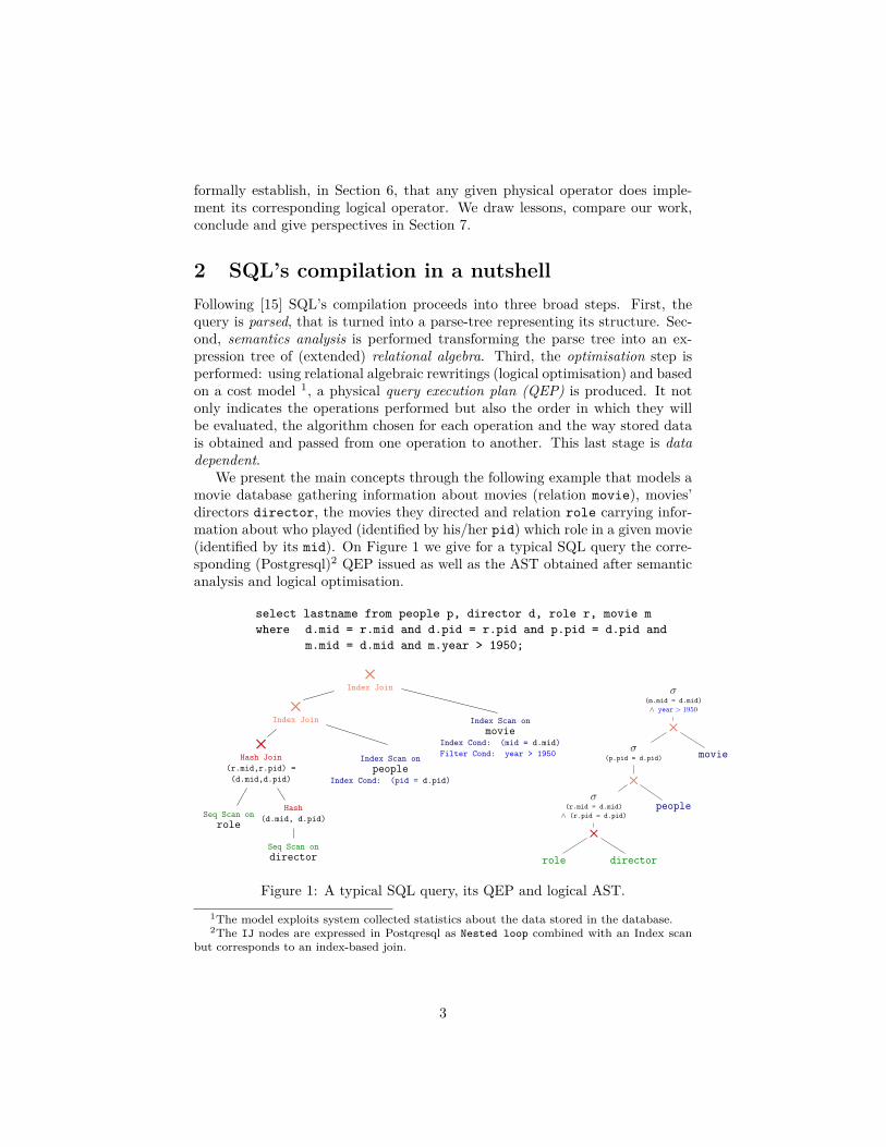
We present the main concepts through the following example that models amovie database gathering information about movies (relation movie), movies’directors director, the movies they directed and relation role carrying infor-mation about who played (identified by his/her pid) which role in a given movie(identified by its mid). On Figure 1 we give for a typical SQL query the corre-sponding (Postgresql)2 QEP issued as well as the AST obtained after semanticanalysis and logical optimisation.

select lastname from people p, director d, role r, movie mwhere d.mid = r.mid and d.pid = r.pid and p.pid = d.pid and

m.mid = d.mid and m.year > 1950;

5Index Join

5Index Join Index Scan on

movieIndex Cond: (mid = d.mid)

Filter Cond: year > 19505

Hash Join

(r.mid,r.pid) =

(d.mid,d.pid)

Index Scan on

peopleIndex Cond: (pid = d.pid)

Seq Scan on

role

Hash

(d.mid, d.pid)

Seq Scan on

director

σ(m.mid = d.mid)

∧ year > 1950

5

movieσ

(p.pid = d.pid)

5

peopleσ

(r.mid = d.mid)

∧ (r.pid = d.pid)

5

role director

Figure 1: A typical SQL query, its QEP and logical AST.1The model exploits system collected statistics about the data stored in the database.2The IJ nodes are expressed in Postqresql as Nested loop combined with an Index scan

but corresponds to an index-based join.

3

The leaves (i.e., relations) are treated by means of access methods such asSeq Scan or Index Scan (in case an index is available); a third access methodusually provided by RDBMS’s is the Sort Scan which orders the elements inthe result according to a given criteria. In the example, relations role anddirector are accessed via Seq Scan, whereas people and movie are accessedthanks to Index Scan. The product of relations in the from part is reorderedand the filtering condition is spread over the relevant (sub-product of) relations.

Intuitively, each physical operator corresponds to one or a combination ofalgebraic operators: σ (selection), × (product), completed with π (projection)and γ (grouping) (see Section 5.1 for their formal semantics).

Conversely, to each operator of the logical plan, σ,×, . . ., potentially cor-responds one or more operators of the physical plan: the underlying databasesystem provides several different algorithm’s implementations. For the crossproduct, for instance, at least four such different algorithms are provided bymainstream systems: Nested Loop, Index Join, Sort Merge Join and HashJoin. For the selection operator the system may use the Filter physical oper-ator.

The situation is made even more complex by the facts that a QEP containssome strategy (top-down, left-most evaluation) and that some physical operatorsare implemented via on-line algorithms. Hence a filtering condition which spansover a cross-product between two operands, in an algebraic expression, maybe used in the corresponding QEP to filter the second one, by inlining thecondition for each tuple of the first operand. This is the case for instancewith the second join of Figure 1 where the second operand is an Index-Scan.Therefore the pattern x×IJ (Index Scan y Index Cond :a = x.a′) correspondsto σy.a=x.a′(x× y).

Unfortunately not all physical operators support the on-line approach andmaterialising partial results (i.e., temporarily storing intermediate results) isneeded: the Materialise physical operator allows to express this in Postgresqlphysical plans. Table 1 summarises our contributions where the colored cellsindicate the Coq specified and implemented operators.

3 A high-level specification for data-centric op-erators

In the data-centric setting, data are mainly collections of values. Such valuescan be combined and enjoy a decidable comparison. Operators allow for ma-nipulating collections, that is to extract data from a collection according to acondition (filter), to iterate over a collection (map), to combine two collections(join) and, last, to aggregate results over a collection (group).

Since collections may be implemented by various means (lists with or withoutdupplicates, AVL, etc), in the following we shall call these implementationscontainerX’s. The content, that is the elements gathered in such a containerX,may be retrieved with the corresponding function contentX and we also make a

4

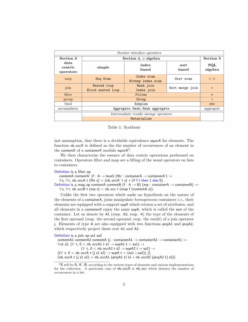
Iterator interface operatorsSection 3 Section 4, φ algebra Section 5

datacentric

operatorssimple index

basedsort

basedSQL

algebra

map Seq ScanIndex scan

Bitmap index scanSort scan r, π

join Nested loopBlock nested loop

Hash joinIndex join

Sort merge join ×

filter Filter σ

group Group γ

bind Subplan envaccumulator Aggregate, Hash, Hash aggregate aggregate

Intermediate results storage operatorsMaterialize

Table 1: Synthesis

last assumption, that there is a decidable equivalence equivX for elements. Thefunction nb– occX is defined as the the number of occurrences of an element inthe contentX of a containerX modulo equivX3.

We then characterise the essence of data centric operations performed oncontainers. Operators filter and map are a lifting of the usual operators on liststo containers.Definition is– a– filter– op

contentA contentA’ (f : A → bool) (fltr : containerA → containerA’) :=∀ s, ∀ t, nb– occA t (fltr s) = (nb– occA’ t s) ∗ (if f t then 1 else 0).

Definition is– a– map– op contentA contentB (f : A → B) (mp : containerA → containerB) :=∀ s, ∀ t, nb– occB t (mp s) = nb– occ t (map f (contentA s)).Unlike the first two operators which make no hypothesis on the nature of

the elements of a containerX, joins manipulate homogeneous containers i.e., theirelements are equipped with a support supX which returns a set of attributes, andall elements in a containerX enjoy the same supX, which is called the sort of thecontainer. Let us denote by A1 (resp. A2, resp. A) the type of the elements ofthe first operand (resp. the second operand, resp. the result) of a join operatorj. Elements of type A are also equipped with two functions projA1 and projA2,which respectively project them over A1 and A2.Definition is– a– join– op sa1 sa2

contentA1 contentA2 contentA (j : containerA1 → containerA2 → containerA) :=∀ s1 s2, (∀ t, 0 < nb– occA1 t s1 → supA1 t = sa1) →

(∀ t, 0 < nb– occA2 t s2 → supA2 t = sa2) →((∀ t, 0 < nb– occA t (j s1 s2) → supA t = (sa1 ∪ sa2))

∧(nb– occA t (j s1 s2) = nb– occA1 (projA1 t) s1 ∗ nb– occA2 (projA2 t) s2))

3X will be A, A’, B, according to the various types of elements and various implementationsfor the collection. A particular case of nb– occX is nb– occ which denotes the number ofoccurrences in a list.

5

∗ (if supA t = (sa1 ∪ sa2) then 1 else 0).Intuitively, joins allow for combining two homogeneous containers by taking

the union of their sort and the product of their occurrence’s functions.The grouping operator, as presented in textbooks [15], partitions, using mk– g,

a container into groups according to a grouping criteria g and then discards somegroups that do not satisfy a filtering condition f. Last for the remaining groupsit builds a new element.Definition is– a– grouping– op (G : Type) (mk– g : G → containerA → list B) grp :=∀ (g : G) (f : B → bool) (build : B → A) (s : containerA) t,nb– occA t (grp g f build s) = nb– occ t (map build (filter f (mk– g g s))).

All the above definitions share a common pattern: they state that the num-ber of occurences nb– occX t (o p s) of an element t in a container built froman operator o applied to some parameters p and some operands s, is equal tofo,p(t, nb– occX (g t) s), where fo,p is a function which depends only on the oper-ator and the parameters. This implies that any two operators satisfying thesame specification is– a– ...– op are interchangeable. For grouping, the situation isslightly more subtle, however the same interchangeability property shall holdsince nb– occA t (grp g f build s)) depends only on t and contentA s for the groupingcriteria used in the following sections.

Tuning those definitions was really challenging: finding the relevant levelof abstraction for containers and contents suitable to host both physical andlogical operators was not intuitive. Even for the most simple one such as filter,we would have expected that the type of containers should be the same for inputand output. It was not possible as we wanted a simple, concise and efficientimplementation.

4 Physical algebraAll physical operators that can be implemented by on-line algorithms rely on acommon iterator interface that allows them to build the next tuple on demand.

4.1 IteratorsA key aspect in our formalisation of physical operators is a specification of sucha common iterator interface together with the properties an iterator needs tosatisfy. We validate this interface by implementing standard iterative physicaloperators, namely sequential scanning, filtering, and nested loop.

Abstract iterator interface An iterator is a data structure that iteratesover a collection of elements to provide them, on demand, one after the other.Following the iterator interface given in [15] and in the same spirit of the for-malisation of cursors presented in [14], we define a cursor as an abstract objectover some type elt of elements that must support three operations: next, thatreturns the next element of the iteration if it exists; has– next, that checks if suchan element does exist; and reset, that restarts the cursor at its beginning. In

6

Coq, this can be modelled as a record4 named Cursor that contains (at least) anabstract type of cursors and these three operations:

Record Cursor (elt : Type) : Type :={ cursor : Type;

next : cursor → result elt ∗ cursor;

has– next : cursor → Prop;reset : cursor → cursor;[...] (∗ Some properties, see below ∗) }.

Due to the immutable nature of Coq objects, the operations next and resetmust return the modified cursor. Moreover, since next must be a total function,a monadic construction is used to wrap the element of type t that it outputs:

Inductive result (A:Type) :=| Result: A → result A

| No– Result: result A| Empty– Cursor: result A.

The constructor Result corresponds to the case where an element can bereturned, and the two constructors No– Result and Empty– Cursor deal with thecases where an element cannot be returned, respectively because it does notmatch some selection condition (see Sec. 4.1) or because the cursor has beenfully iterated over.

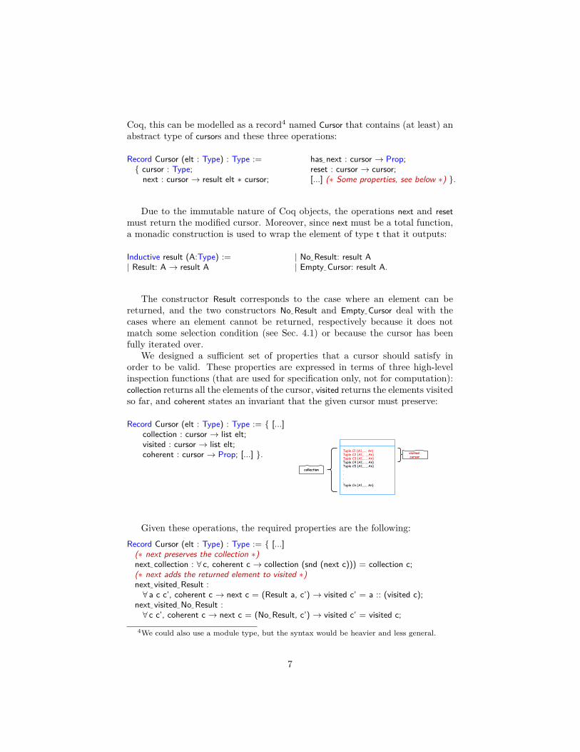
We designed a sufficient set of properties that a cursor should satisfy inorder to be valid. These properties are expressed in terms of three high-levelinspection functions (that are used for specification only, not for computation):collection returns all the elements of the cursor, visited returns the elements visitedso far, and coherent states an invariant that the given cursor must preserve:

Record Cursor (elt : Type) : Type := { [...]collection : cursor → list elt;visited : cursor → list elt;coherent : cursor → Prop; [...] }.

Given these operations, the required properties are the following:Record Cursor (elt : Type) : Type := { [...]

(∗ next preserves the collection ∗)next– collection : ∀ c, coherent c → collection (snd (next c))) = collection c;(∗ next adds the returned element to visited ∗)next– visited– Result :∀ a c c’, coherent c → next c = (Result a, c’) → visited c’ = a :: (visited c);

next– visited– No– Result :∀ c c’, coherent c → next c = (No– Result, c’) → visited c’ = visited c;

4We could also use a module type, but the syntax would be heavier and less general.

7

next– visited– Empty– Cursor :∀ c c’, coherent c → next c = (Empty– Cursor, c’) → visited c’ = visited c;

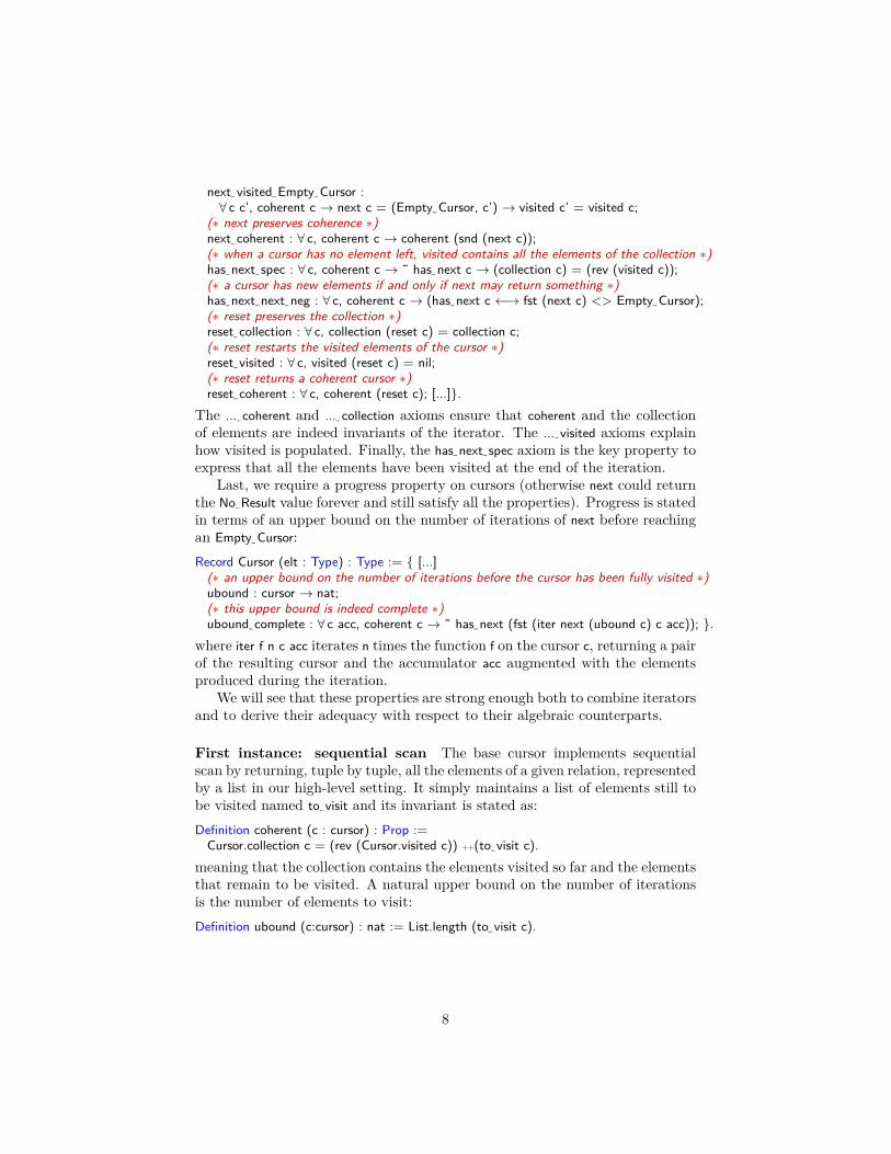
(∗ next preserves coherence ∗)next– coherent : ∀ c, coherent c → coherent (snd (next c));(∗ when a cursor has no element left, visited contains all the elements of the collection ∗)has– next– spec : ∀ c, coherent c → ˜ has– next c → (collection c) = (rev (visited c));(∗ a cursor has new elements if and only if next may return something ∗)has– next– next– neg : ∀ c, coherent c → (has– next c ←→ fst (next c) <> Empty– Cursor);(∗ reset preserves the collection ∗)reset– collection : ∀ c, collection (reset c) = collection c;(∗ reset restarts the visited elements of the cursor ∗)reset– visited : ∀ c, visited (reset c) = nil;(∗ reset returns a coherent cursor ∗)reset– coherent : ∀ c, coherent (reset c); [...]}.

The ...– coherent and ...– collection axioms ensure that coherent and the collectionof elements are indeed invariants of the iterator. The ...– visited axioms explainhow visited is populated. Finally, the has– next– spec axiom is the key property toexpress that all the elements have been visited at the end of the iteration.

Last, we require a progress property on cursors (otherwise next could returnthe No– Result value forever and still satisfy all the properties). Progress is statedin terms of an upper bound on the number of iterations of next before reachingan Empty– Cursor:Record Cursor (elt : Type) : Type := { [...]

(∗ an upper bound on the number of iterations before the cursor has been fully visited ∗)ubound : cursor → nat;(∗ this upper bound is indeed complete ∗)ubound– complete : ∀ c acc, coherent c → ˜ has– next (fst (iter next (ubound c) c acc)); }.

where iter f n c acc iterates n times the function f on the cursor c, returning a pairof the resulting cursor and the accumulator acc augmented with the elementsproduced during the iteration.

We will see that these properties are strong enough both to combine iteratorsand to derive their adequacy with respect to their algebraic counterparts.

First instance: sequential scan The base cursor implements sequentialscan by returning, tuple by tuple, all the elements of a given relation, representedby a list in our high-level setting. It simply maintains a list of elements still tobe visited named to– visit and its invariant is stated as:Definition coherent (c : cursor) : Prop :=

Cursor.collection c = (rev (Cursor.visited c)) ++(to– visit c).meaning that the collection contains the elements visited so far and the elementsthat remain to be visited. A natural upper bound on the number of iterationsis the number of elements to visit:Definition ubound (c:cursor) : nat := List.length (to– visit c).

8

Second instance: filter Filtering a cursor returns the same cursor, but witha different function next and accordingly different specification functions. Givena property on the elements f : elt → bool, the function next filters elements of theunderlying cursor:Definition next (c : cursor) : result elt ∗ cursor :=

match Cursor.next c with| (Result e, c’) ⇒ if f e then (Result e, c’) else (No– Result, c’)| rc’ ⇒ rc’end.

This is where No– Result is introduced when the condition is not met. Accordingly,the functions collection and visited are the filtered collection and visited of theunderlying cursor and an upper bound on the number of iterations is the upperbound of the underlying cursor:Definition collection (c : cursor) := List.filter f (Cursor.collection c).Definition visited (c : cursor) := List.filter f (Cursor.visited c).Definition ubound (q : cursor) : nat := Cursor.ubound q.

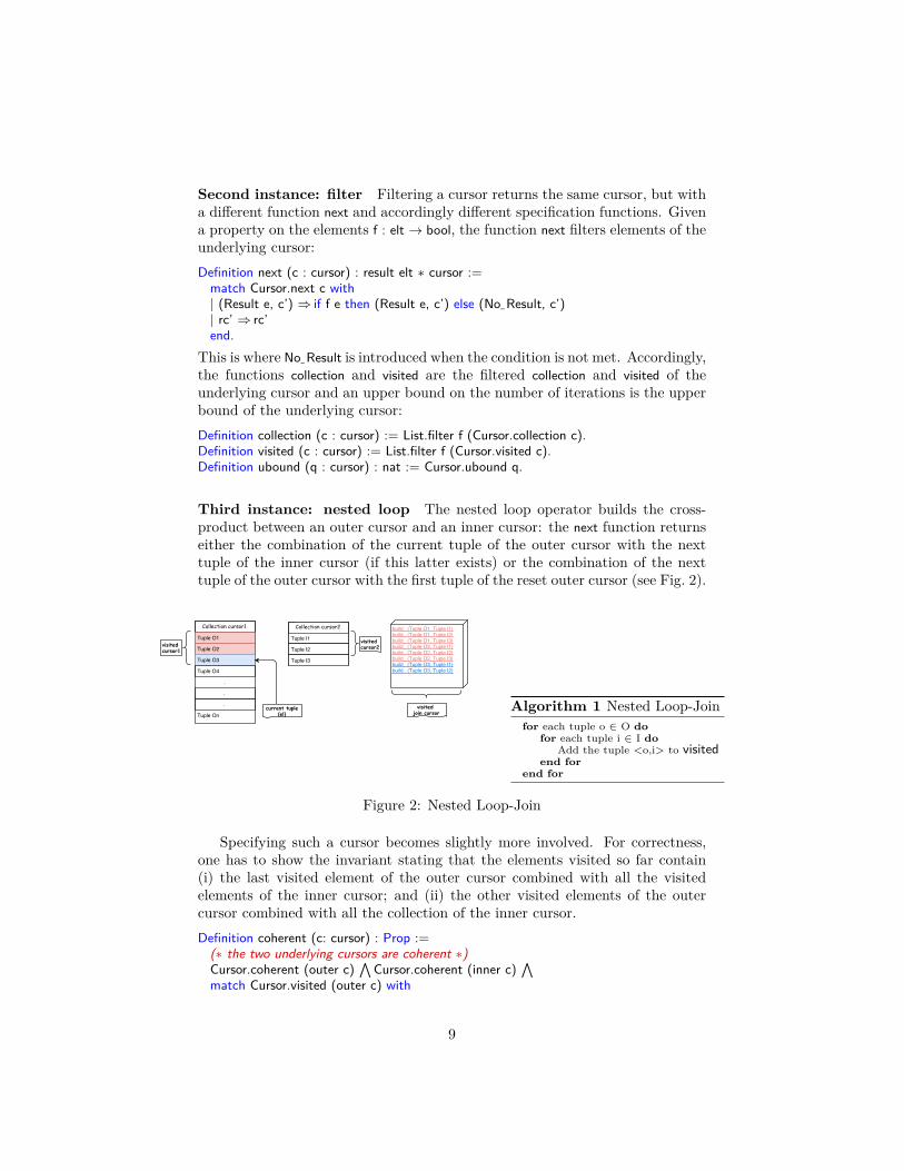
Third instance: nested loop The nested loop operator builds the cross-product between an outer cursor and an inner cursor: the next function returnseither the combination of the current tuple of the outer cursor with the nexttuple of the inner cursor (if this latter exists) or the combination of the nexttuple of the outer cursor with the first tuple of the reset outer cursor (see Fig. 2).

Algorithm 1 Nested Loop-Joinfor each tuple o ∈ O do

for each tuple i ∈ I doAdd the tuple <o,i> to visited

end forend for

Figure 2: Nested Loop-Join

Specifying such a cursor becomes slightly more involved. For correctness,one has to show the invariant stating that the elements visited so far contain(i) the last visited element of the outer cursor combined with all the visitedelements of the inner cursor; and (ii) the other visited elements of the outercursor combined with all the collection of the inner cursor.Definition coherent (c: cursor) : Prop :=

(∗ the two underlying cursors are coherent ∗)Cursor.coherent (outer c)

∧Cursor.coherent (inner c)

∧match Cursor.visited (outer c) with

9

(∗ if the outer cursor has not been visited yet, so as the inner cursor ∗)| nil ⇒ visited c = nil

∧Cursor.visited (inner c) = nil

(∗ otherwise, the visited elements are a partial cross−product ∗)| el :: li ⇒ visited c = (cross (el::nil) (Cursor.visited (inner c))) ++

(cross li (rev (Cursor.collection (inner c))))end.

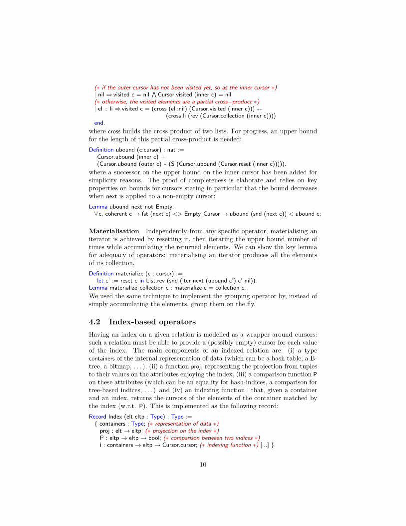
where cross builds the cross product of two lists. For progress, an upper boundfor the length of this partial cross-product is needed:Definition ubound (c:cursor) : nat :=

Cursor.ubound (inner c) +(Cursor.ubound (outer c) ∗ (S (Cursor.ubound (Cursor.reset (inner c))))).

where a successor on the upper bound on the inner cursor has been added forsimplicity reasons. The proof of completeness is elaborate and relies on keyproperties on bounds for cursors stating in particular that the bound decreaseswhen next is applied to a non-empty cursor:Lemma ubound– next– not– Empty:∀ c, coherent c → fst (next c) <> Empty– Cursor → ubound (snd (next c)) < ubound c;

Materialisation Independently from any specific operator, materialising aniterator is achieved by resetting it, then iterating the upper bound number oftimes while accumulating the returned elements. We can show the key lemmafor adequacy of operators: materialising an iterator produces all the elementsof its collection.Definition materialize (c : cursor) :=

let c’ := reset c in List.rev (snd (iter next (ubound c’) c’ nil)).Lemma materialize– collection c : materialize c = collection c.We used the same technique to implement the grouping operator by, instead ofsimply accumulating the elements, group them on the fly.

4.2 Index-based operatorsHaving an index on a given relation is modelled as a wrapper around cursors:such a relation must be able to provide a (possibly empty) cursor for each valueof the index. The main components of an indexed relation are: (i) a typecontainers of the internal representation of data (which can be a hash table, a B-tree, a bitmap, . . . ), (ii) a function proj, representing the projection from tuplesto their values on the attributes enjoying the index, (iii) a comparison function Pon these attributes (which can be an equality for hash-indices, a comparison fortree-based indices, . . . ) and (iv) an indexing function i that, given a containerand an index, returns the cursors of the elements of the container matched bythe index (w.r.t. P). This is implemented as the following record:Record Index (elt eltp : Type) : Type :={ containers : Type; (∗ representation of data ∗)

proj : elt → eltp; (∗ projection on the index ∗)P : eltp → eltp → bool; (∗ comparison between two indices ∗)i : containers → eltp → Cursor.cursor; (∗ indexing function ∗) [...] }.

10

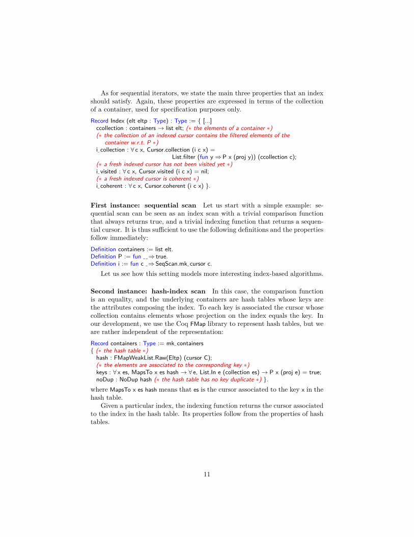
As for sequential iterators, we state the main three properties that an indexshould satisfy. Again, these properties are expressed in terms of the collectionof a container, used for specification purposes only.Record Index (elt eltp : Type) : Type := { [...]

ccollection : containers → list elt; (∗ the elements of a container ∗)(∗ the collection of an indexed cursor contains the filtered elements of the

container w.r.t. P ∗)i– collection : ∀ c x, Cursor.collection (i c x) =

List.filter (fun y ⇒P x (proj y)) (ccollection c);(∗ a fresh indexed cursor has not been visited yet ∗)i– visited : ∀ c x, Cursor.visited (i c x) = nil;(∗ a fresh indexed cursor is coherent ∗)i– coherent : ∀ c x, Cursor.coherent (i c x) }.

First instance: sequential scan Let us start with a simple example: se-quential scan can be seen as an index scan with a trivial comparison functionthat always returns true, and a trivial indexing function that returns a sequen-tial cursor. It is thus sufficient to use the following definitions and the propertiesfollow immediately:Definition containers := list elt.Definition P := fun – –⇒ true.Definition i := fun c –⇒SeqScan.mk– cursor c.

Let us see how this setting models more interesting index-based algorithms.

Second instance: hash-index scan In this case, the comparison functionis an equality, and the underlying containers are hash tables whose keys arethe attributes composing the index. To each key is associated the cursor whosecollection contains elements whose projection on the index equals the key. Inour development, we use the Coq FMap library to represent hash tables, but weare rather independent of the representation:Record containers : Type := mk– containers{ (∗ the hash table ∗)

hash : FMapWeakList.Raw(Eltp) (cursor C);(∗ the elements are associated to the corresponding key ∗)keys : ∀ x es, MapsTo x es hash → ∀ e, List.In e (collection es) → P x (proj e) = true;noDup : NoDup hash (∗ the hash table has no key duplicate ∗) }.

where MapsTo x es hash means that es is the cursor associated to the key x in thehash table.

Given a particular index, the indexing function returns the cursor associatedto the index in the hash table. Its properties follow from the properties of hashtables.

11

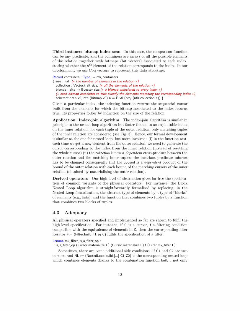
Third instance: bitmap-index scan In this case, the comparison functioncan be any predicate, and the containers are arrays of all the possible elementsof the relation together with bitmaps (bit vectors) associated to each index,stating whether the nth element of the relation corresponds to the index. In ourdevelopment, we use Coq vectors to represent this data structure:Record containers : Type := mk– containers{ size : nat; (∗ the number of elements in the relation ∗)

collection : Vector.t elt size; (∗ all the elements of the relation ∗)bitmap : eltp → Bvector size;(∗ a bitmap associated to every index ∗)(∗ each bitmap associates to true exactly the elements matching the corresponding index ∗)coherent : ∀ n x0, nth (bitmap x0) n = P x0 (proj (nth collection n)) }.

Given a particular index, the indexing function returns the sequential cursorbuilt from the elements for which the bitmap associated to the index returnstrue. Its properties follow by induction on the size of the relation.

Application: Index-join algorithm The index-join algorithm is similar inprinciple to the nested loop algorithm but faster thanks to an exploitable indexon the inner relation: for each tuple of the outer relation, only matching tuplesof the inner relation are considered (see Fig. 3). Hence, our formal developmentis similar as the one for nested loop, but more involved: (i) in the function next,each time we get a new element from the outer relation, we need to generate thecursor corresponding to the index from the inner relation (instead of resettingthe whole cursor) (ii) the collection is now a dependent cross-product between theouter relation and the matching inner tuples; the invariant predicate coherenthas to be changed consequently (iii) the ubound is a dependent product of thebound of the outer relation with each bound of the matching cursors of the innerrelation (obtained by materialising the outer relation).

Derived operators Our high level of abstraction gives for free the specifica-tion of common variants of the physical operators. For instance, the BlockNested Loop algorithm is straightforwardly formalised by replacing, in theNested Loop formalisation, the abstract type of elements by a type of “blocks”of elements (e.g., lists), and the function that combines two tuples by a functionthat combines two blocks of tuples.

4.3 AdequacyAll physical operators specified and implemented so far are shown to fulfil thehigh-level specification. For instance, if C is a cursor, f a filtering conditioncompatible with the equivalence of elements in C, then the corresponding filteriterator F:= (Filter.build f f– eq C) fulfils the specification of a filter:Lemma mk– filter– is– a– filter– op :

is– a– filter– op (Cursor.materialize C) (Cursor.materialize F) f (Filter.mk– filter F).Sometimes, there are some additional side conditions: if C1 and C2 are two

cursors, and NL := (NestedLoop.build [...] C1 C2) is the corresponding nested loopwhich combines elements thanks to the combination function build– , not only

12

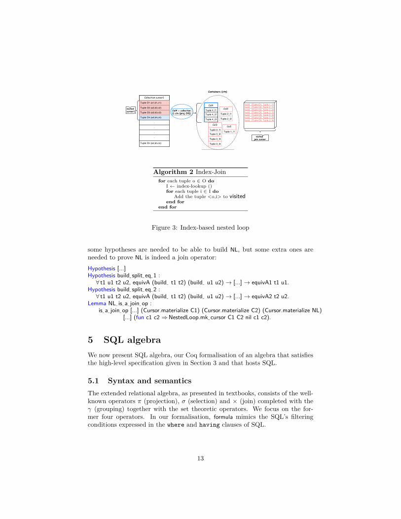
Algorithm 2 Index-Joinfor each tuple o ∈ O do

I ← index-lookup ()for each tuple i ∈ I do

Add the tuple <o,i> to visitedend for

end for

Figure 3: Index-based nested loop

some hypotheses are needed to be able to build NL, but some extra ones areneeded to prove NL is indeed a join operator:Hypothesis [...]Hypothesis build– split– eq– 1 :∀ t1 u1 t2 u2, equivA (build– t1 t2) (build– u1 u2) → [...] → equivA1 t1 u1.

Hypothesis build– split– eq– 2 :∀ t1 u1 t2 u2, equivA (build– t1 t2) (build– u1 u2) → [...] → equivA2 t2 u2.

Lemma NL– is– a– join– op :is– a– join– op [...] (Cursor.materialize C1) (Cursor.materialize C2) (Cursor.materialize NL)

[...] (fun c1 c2 ⇒NestedLoop.mk– cursor C1 C2 nil c1 c2).

5 SQL algebraWe now present SQL algebra, our Coq formalisation of an algebra that satisfiesthe high-level specification given in Section 3 and that hosts SQL.

5.1 Syntax and semanticsThe extended relational algebra, as presented in textbooks, consists of the well-known operators π (projection), σ (selection) and × (join) completed with theγ (grouping) together with the set theoretic operators. We focus on the for-mer four operators. In our formalisation, formula mimics the SQL’s filteringconditions expressed in the where and having clauses of SQL.

13

Inductive query : Type :=| Q– Table : relname → query| Q– Set :

set– op → query → query → query| Q– Join : query → query → query| Q– Pi : list select → query → query| Q– Sigma : formula → query → query| Q– Gamma :

list term → formula → list select →query → query

with formula : Type :=| Q– Conj :

and– or → formula → formula →

formula| Q– Not : formula → formula| Q– Atom : atom → formula

with atom : Type :=| Q– True| Q– Pred : predicate → list term →

atom| Q– Quant :

quantifier → predicate → list term →query → atom

| Q– In : list select → query → atom| Q– Exists : query → atom.

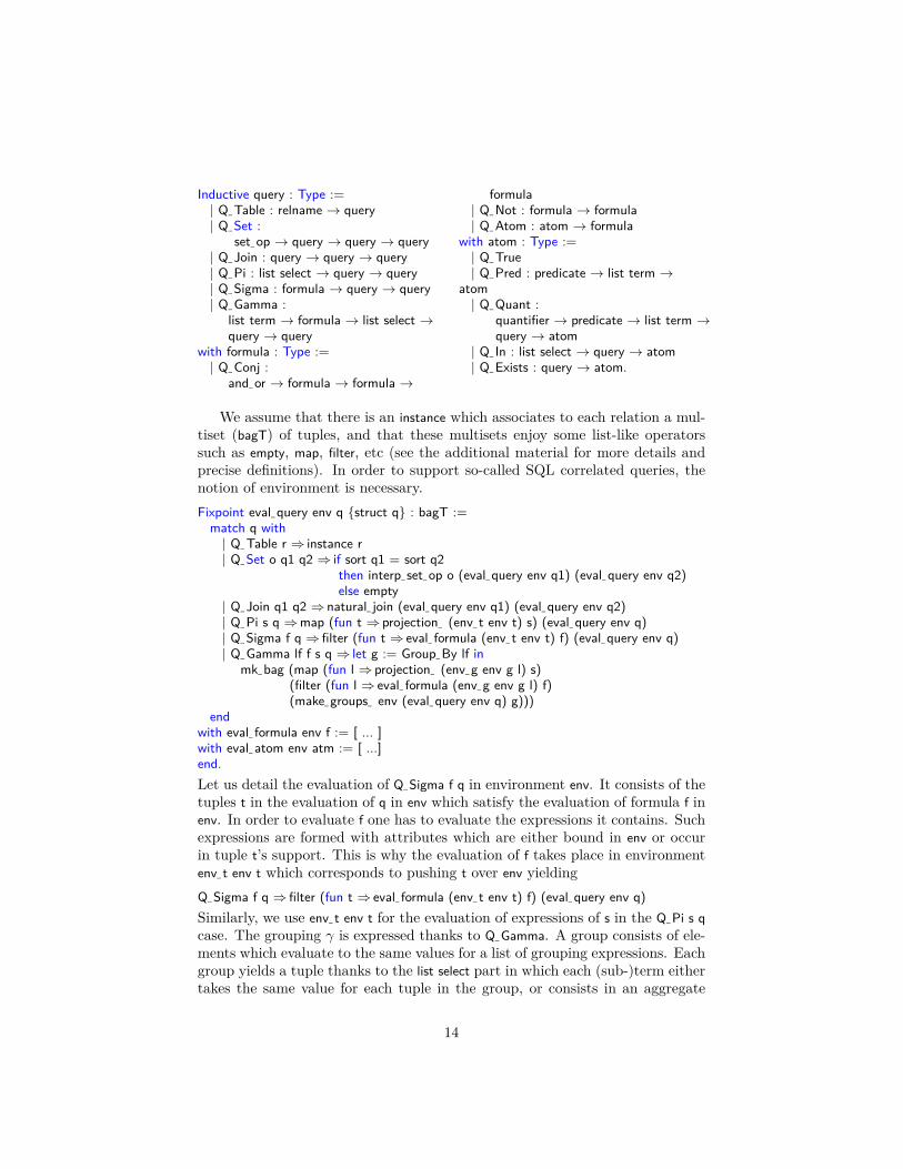
We assume that there is an instance which associates to each relation a mul-tiset (bagT) of tuples, and that these multisets enjoy some list-like operatorssuch as empty, map, filter, etc (see the additional material for more details andprecise definitions). In order to support so-called SQL correlated queries, thenotion of environment is necessary.Fixpoint eval– query env q {struct q} : bagT :=

match q with| Q– Table r ⇒ instance r| Q– Set o q1 q2 ⇒ if sort q1 = sort q2

then interp– set– op o (eval– query env q1) (eval– query env q2)else empty

| Q– Join q1 q2 ⇒ natural– join (eval– query env q1) (eval– query env q2)| Q– Pi s q ⇒map (fun t ⇒ projection– (env– t env t) s) (eval– query env q)| Q– Sigma f q ⇒ filter (fun t ⇒ eval– formula (env– t env t) f) (eval– query env q)| Q– Gamma lf f s q ⇒ let g := Group– By lf in

mk– bag (map (fun l ⇒ projection– (env– g env g l) s)(filter (fun l ⇒ eval– formula (env– g env g l) f)(make– groups– env (eval– query env q) g)))

endwith eval– formula env f := [ ... ]with eval– atom env atm := [ ...]end.Let us detail the evaluation of Q– Sigma f q in environment env. It consists of thetuples t in the evaluation of q in env which satisfy the evaluation of formula f inenv. In order to evaluate f one has to evaluate the expressions it contains. Suchexpressions are formed with attributes which are either bound in env or occurin tuple t’s support. This is why the evaluation of f takes place in environmentenv– t env t which corresponds to pushing t over env yieldingQ– Sigma f q ⇒ filter (fun t ⇒ eval– formula (env– t env t) f) (eval– query env q)Similarly, we use env– t env t for the evaluation of expressions of s in the Q– Pi s qcase. The grouping γ is expressed thanks to Q– Gamma. A group consists of ele-ments which evaluate to the same values for a list of grouping expressions. Eachgroup yields a tuple thanks to the list select part in which each (sub-)term eithertakes the same value for each tuple in the group, or consists in an aggregate

14

expression. This usual definition (see for instance [15]) is not enough to handleSQL’s having conditions, as having directly operates on the group that carrymore information than the corresponding tuple. This is why Q– Gamma has alsoa formula operand. Thus the corresponding expression for query

select avg(a1) as avg a1, sum(b1) as sum b1 from t1group by a1+b1, 3*b1 having a1 + b1 > 3 + avg(c1);

is Q Gamma [a1 + b1; 3*b1] (Q Atom (Q Pred > [a1 + b1; 3 + avg(c1)]))[Select As avg(a1) avg a1; Select As sum(b1) sum b1] (Q table t1)

5.2 AdequacyThe following lemmas assess that SQL algebra is a realisation of our high-levelspecification. Note that, in the context of SQL algebra the notion of tuplecorresponds to the high-level notion of elements’ type X, finite bag correspondsto the high-level notion of containerX and elements to contentX.Lemma Q– Sigma– is– a– filter– op :∀ env f,

is– a– filter– op [...](∗ contentA := fun q ⇒Febag.elements BTupleT (eval– query env q) ∗)(∗ contentA’ := fun q ⇒Febag.elements BTupleT (eval– query env q) ∗)(fun t ⇒ eval– formula (env– t env t) f)(fun q ⇒Q– Sigma f q).

Lemma Q– Join– is– a– join– op : ∀ env s1 s2,let Q– Join q1 q2 := Q– Join q1 q2 inis– a– join– op (∗ contentA1 := fun q ⇒ elements (eval– query env q) ∗)

(∗ contentA2 := fun q ⇒ elements (eval– query env q) ∗)(∗ contentA := fun q ⇒ elements (eval– query env q) ∗) [...] s1 s2 Q– Join.

Lemma Q– Gamma– is– a– grouping– op : ∀ env g f s ,let eval– s l := projection– (env– g env (Group– By g) l) (Select– List s) inlet eval– f l := eval– formula (env– g env (Group– By g) l) f inlet mk– grp g q := partition– list– expr (elements (eval– query env q))

(map (fun f t ⇒ interp– funterm (env– t env t) f) g) inlet Q– Gamma g f s q := eval– query env (Q– Gamma g f s q) inis– a– grouping– op [...] mk– grp g eval– f eval– s (Q– Gamma g f s).

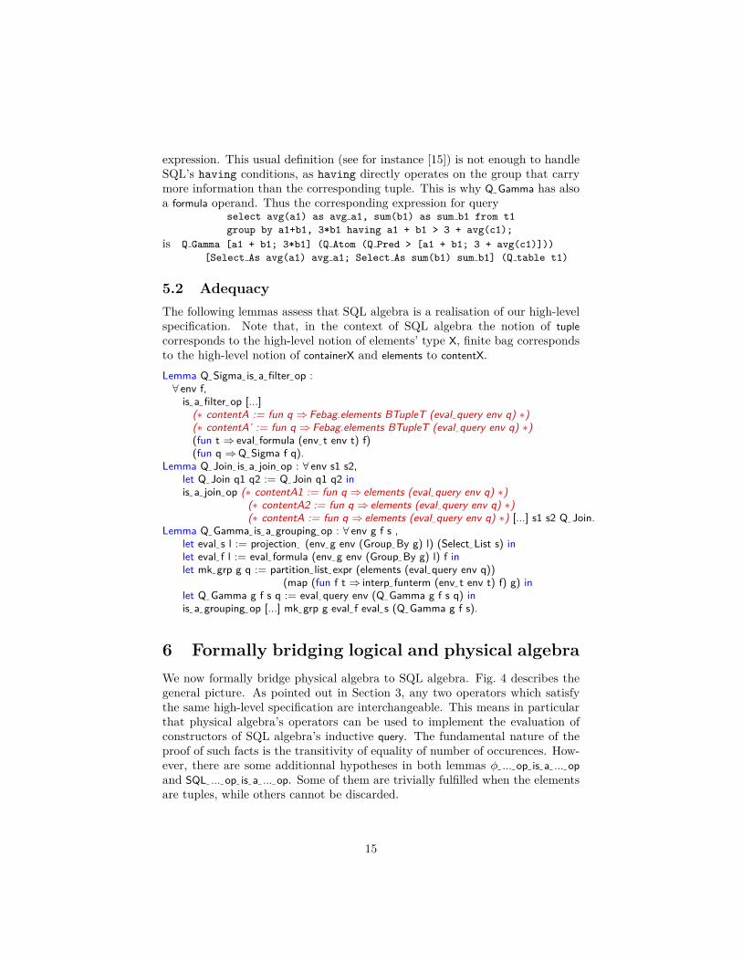
6 Formally bridging logical and physical algebraWe now formally bridge physical algebra to SQL algebra. Fig. 4 describes thegeneral picture. As pointed out in Section 3, any two operators which satisfythe same high-level specification are interchangeable. This means in particularthat physical algebra’s operators can be used to implement the evaluation ofconstructors of SQL algebra’s inductive query. The fundamental nature of theproof of such facts is the transitivity of equality of number of occurences. How-ever, there are some additionnal hypotheses in both lemmas φ– ...– op– is– a– ...– opand SQL– ...– op– is– a– ...– op. Some of them are trivially fulfilled when the elementsare tuples, while others cannot be discarded.

15

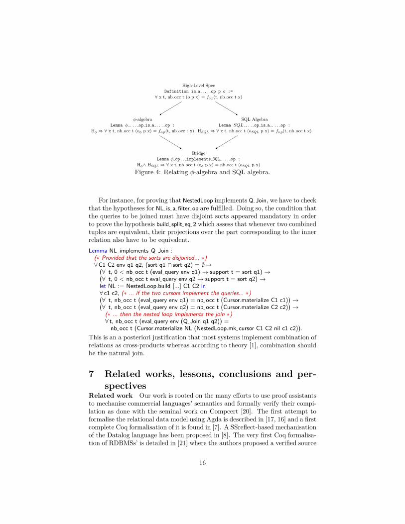
High-Level SpecDefinition is a ... op p o :=

∀ x t, nb occ t (o p x) = fo,p(t, nb occ t x)

φ-algebraLemma φ ... op is a ... op :

Hφ ⇒ ∀ x t, nb occ t (oφ p x) = fo,p(t, nb occ t x)

SQL AlgebraLemma SQL ... op is a ... op :

HSQL ⇒ ∀ x t, nb occ t (oSQL p x) = fo,p(t, nb occ t x)

BridgeLemma φ op_.. implements SQL ... op :

Hφ∧ HSQL ⇒ ∀ x t, nb occ t (oφ p x) = nb occ t (oSQL p x)

Figure 4: Relating φ-algebra and SQL algebra.

For instance, for proving that NestedLoop implements Q– Join, we have to checkthat the hypotheses for NL– is– a– filter– op are fulfilled. Doing so, the condition thatthe queries to be joined must have disjoint sorts appeared mandatory in orderto prove the hypothesis build– split– eq– 2 which assess that whenever two combinedtuples are equivalent, their projections over the part corresponding to the innerrelation also have to be equivalent.Lemma NL– implements– Q– Join :

(∗ Provided that the sorts are disjoined... ∗)∀C1 C2 env q1 q2, (sort q1 ∩ sort q2) = ∅→

(∀ t, 0 < nb– occ t (eval– query env q1) → support t = sort q1) →(∀ t, 0 < nb– occ t eval– query env q2 → support t = sort q2) →let NL := NestedLoop.build [...] C1 C2 in∀ c1 c2, (∗ ... if the two cursors implement the queries... ∗)(∀ t, nb– occ t (eval– query env q1) = nb– occ t (Cursor.materialize C1 c1)) →(∀ t, nb– occ t (eval– query env q2) = nb– occ t (Cursor.materialize C2 c2)) →

(∗ ... then the nested loop implements the join ∗)∀ t, nb– occ t (eval– query env (Q– Join q1 q2)) =

nb– occ t (Cursor.materialize NL (NestedLoop.mk– cursor C1 C2 nil c1 c2)).This is an a posteriori justification that most systems implement combination ofrelations as cross-products whereas according to theory [1], combination shouldbe the natural join.

7 Related works, lessons, conclusions and per-spectives

Related work Our work is rooted on the many efforts to use proof assistantsto mechanise commercial languages’ semantics and formally verify their compi-lation as done with the seminal work on Compcert [20]. The first attempt toformalise the relational data model using Agda is described in [17, 16] and a firstcomplete Coq formalisation of it is found in [7]. A SSreflect-based mechanisationof the Datalog language has been proposed in [8]. The very first Coq formalisa-tion of RDBMSs’ is detailed in [21] where the authors proposed a verified source

16

to source compiler for (a small subset) of SQL. More recently, in [3, 4] a Coqmodelisation of the nested relational algebra is provided to assign a semantics todata-centric languages among which SQL. Regarding logical optimisation, themost in depth proposal is addressed in [10] where the authors describe a tool todecide whether two SQL queries are equivalent. However, none of these worksconsider specifying and verifying the low-level aspects of SQL’s compilation andexecution as we did. Our work is, thus, complementary to theirs and one per-spective could be to join our efforts along the line of formalising data-centricsystems.

Lessons, conclusions and perspectives We used the Coq proof assistantto specify and verify the low level layer of an RDBMS as well as SQL’s com-pilation’s physical optimisation: fundamental steps towards mechanising SQL’scompilation chain.

While formalising all this, we learnt the following lessons: (i) not only findingthe right invariants for physical operators was really involved but proving them(in particular termination for nested loop) was indeed subtle. This is due to theinherent difficulty to design on-line versions of even trivial off-line algorithms.(ii) we are even more convinced by the relevance of designing such a high-levelspecification that opens the way for accounting other data-centric languages.More precisely, we first formalised SQL algebra then the physical one, this im-plied revising the specification: in particular the introduction of containersX wasmade. Then, while bridging both formalisms we slightly modified the specifica-tion but without questionning our fundamental choices about abstracting overcollections using containersX, only hypotheses were slightly tuned. (iii) The needfor higher-order and polymorphism was mandatory both for the specificationand physical algebra modelisation. This prevented us from using deductive ver-ification tools such as Why3 [13] for instance: it was quite difficult to write downthe algorithms and their invariants in this setting, even worse the automatedprovers were of no use to discharge the proof obligations. We tried tuning theinvariants to help provers, without success. Hence our claim is that it is easierto directly use a proof assistant, where one has the control over the statementswhich have to be proven. (iv) The last point is that we experimented recordsversus modules: records are simpler to use than modules in our formalisation(no need of definitions’ unfolding, no need of intermediate inductive types fortechnical reasons), the counterpart being that modules in the standard Coq li-brary, such as FSets or FMaps were not directy usable. The nice feature whichallows to hide part of their contents through module subtyping was not neededhere.

There are many points still to be addressed. In the very short term weplan to specify the missing operators of Table 1 and enrich the physical alge-bra with more fancy algorithms. Along this line two directions remain to beexplored. In our development, the emphasis was put on specification ratherthan performance. In [18] an Isabelle formalization of the complexity of on-linealgorithms is proposed and we shall rely on it to formally assess the complexityof the algorithms presented so far. Even if we carefully separated functions used

17

in specification (such as collection, coherent, . . . ) from the concrete algorithms,these latter are defined in the functional language of Coq using higher-orderdata structures. We plan to refine these algorithms into more efficient versions,in particular that manipulate the memory. We plan to rely on CertiCoq [2] inorder to produce fully certified C code. Last, we are confident that our specifi-cation is general enough to host various data-centric languages and will providea framework for data-centric languages interoperability which is our long termgoal.

References[1] S. Abiteboul, R. Hull, and V. Vianu. Foundations of Databases. Addison-

Wesley, 1995.

[2] A. Anand, A. Appel, G. Morrisett, Z. Paraskevopoulou, R. Pollack,O. Belanger-Savary, M. Sozeau, and M. Weaver. Certicoq: A verified com-piler for coq. In The Third International Workshop on Coq for ProgrammingLanguages (CoqPL), 2017.

[3] J. S. Auerbach, M. Hirzel, L. Mandel, A. Shinnar, and J. Simeon. Han-dling environments in a nested relational algebra with combinators and animplementation in a verified query compiler. In S. Salihoglu, W. Zhou,R. Chirkova, J. Yang, and D. Suciu, editors, Proceedings of the 2017 ACMInternational Conference on Management of Data, SIGMOD Conference2017, Chicago, IL, USA, May 14-19, 2017, pages 1555–1569. ACM, 2017.

[4] J. S. Auerbach, M. Hirzel, L. Mandel, A. Shinnar, and J. Simeon. Q*cert:A platform for implementing and verifying query compilers. In Proceed-ings of the 2017 ACM International Conference on Management of Data,SIGMOD Conference 2017, Chicago, IL, USA, May 14-19, 2017, pages1703–1706, 2017.

[5] P. Bailis, J. M. Hellerstein, and M. Stonebraker, editors. Readings inDatabase Systems, 5th Edition. 2015.

[6] V. Benzaken and E. Contejean. A Coq mechanised executable algebraicsemantics for real life SQL queries. Submitted for publication, 2018.

[7] V. Benzaken, E. Contejean, and S. Dumbrava. A Coq Formalization ofthe Relational Data Model. In 23rd European Symposium on Programming(ESOP), 2014.

[8] V. Benzaken, E. Contejean, and S. Dumbrava. Certifying standard andstratified datalog inference engines in ssreflect. In M. Ayala-Rincon andC. Munoz, editors, 8th International Conference on Interactive TheoremProving, volume 10499. Springer, 2017.

18

[9] D. D. Chamberlin and R. F. Boyce. SEQUEL: A structured english querylanguage. In R. Rustin, editor, Proceedings of 1974 ACM-SIGMOD Work-shop on Data Description, Access and Control, Ann Arbor, Michigan, May1-3, 1974, 2 Volumes, pages 249–264. ACM, 1974.

[10] S. Chu, K. Weitz, A. Cheung, and D. Suciu. Hottsql: Proving queryrewrites with univalent sql semantics. In Proceedings of the 38th ACMSIGPLAN Conference on Programming Language Design and Implemen-tation, PLDI 2017, pages 510–524, New York, NY, USA, 2017. ACM.

[11] E. F. Codd. A relational model of data for large shared data banks. Com-mun. ACM, 13(6):377–387, 1970.

[12] R. Elmasri and S. B. Navathe. Fundamentals of Database Systems, 2ndEdition. Benjamin/Cummings, 1994.

[13] J.-C. Filliatre and A. Paskevich. Why3 - where programs meet provers. InM. Felleisen and P. Gardner, editors, Programming Languages and Systems- 22nd European Symposium on Programming, ESOP 2013, Held as Partof the European Joint Conferences on Theory and Practice of Software,ETAPS 2013, Rome, Italy, March 16-24, 2013. Proceedings, volume 7792of Lecture Notes in Computer Science, pages 125–128. Springer, 2013.

[14] J.-C. Filliatre and M. Pereira. Iterer avec confiance. In Journees Franco-phones des Langages Applicatifs, Saint-Malo, France, Jan. 2016.

[15] H. Garcia-Molina, J. D. Ullman, and J. Widom. Database systems - thecomplete book (2. ed.). Pearson Education, 2009.

[16] C. Gonzalia. Towards a formalisation of relational database theory in con-structive type theory. In R. Berghammer, B. Moller, and G. Struth, editors,RelMiCS, volume 3051 of LNCS, pages 137–148. Springer, 2003.

[17] C. Gonzalia. Relations in Dependent Type Theory. PhD thesis, ChalmersGoteborg University, 2006.

[18] M. P. L. Haslbeck and T. Nipkow. Verified Analysis of List Update Algo-rithms. In A. Lal, S. Akshay, S. Saurabh, and S. Sen, editors, 36th IARCSAnnual Conference on Foundations of Software Technology and Theoreti-cal Computer Science (FSTTCS 2016), volume 65 of Leibniz InternationalProceedings in Informatics (LIPIcs), pages 49:1–49:15, Dagstuhl, Germany,2016. Schloss Dagstuhl–Leibniz-Zentrum fuer Informatik.

[19] R. M. Karp. On-line algorithms versus off-line algorithms: How muchis it worth to know the future? In J. van Leeuwen, editor, Algorithms,Software, Architecture - Information Processing ’92, Volume 1, Proceedingsof the IFIP 12th World Computer Congress, Madrid, Spain, 7-11 September1992, volume A-12 of IFIP Transactions, pages 416–429. North-Holland,1992.

19

[20] X. Leroy. A formally verified compiler back-end. J. Autom. Reasoning,43(4):363–446, 2009.

[21] G. Malecha, G. Morrisett, A. Shinnar, and R. Wisnesky. Toward a verifiedrelational database management system. In ACM Int. Conf. POPL, 2010.

[22] G. Moerkotte. Building query compilers. http://pi3.informatik.uni-mannheim.de/ moer/querycompiler.pdf.

[23] R. Ramakrishnan and J. Gehrke. Database management systems (3. ed.).McGraw-Hill, 2003.

[24] P. G. Selinger, M. M. Astrahan, D. D. Chamberlin, R. A. Lorie, and T. G.Price. Access path selection in a relational database management system.In Proceedings of the 1979 ACM SIGMOD International Conference onManagement of Data, Boston, Massachusetts, May 30 - June 1., pages23–34, 1979.

[25] The Coq Development Team. The Coq Proof Assistant Reference Manual,2010. http://coq.inria.fr.

[26] The Isabelle Development Team. The Isabelle Interactive Theorem Prover,2010. https://isabelle.in.tum.de/.

20

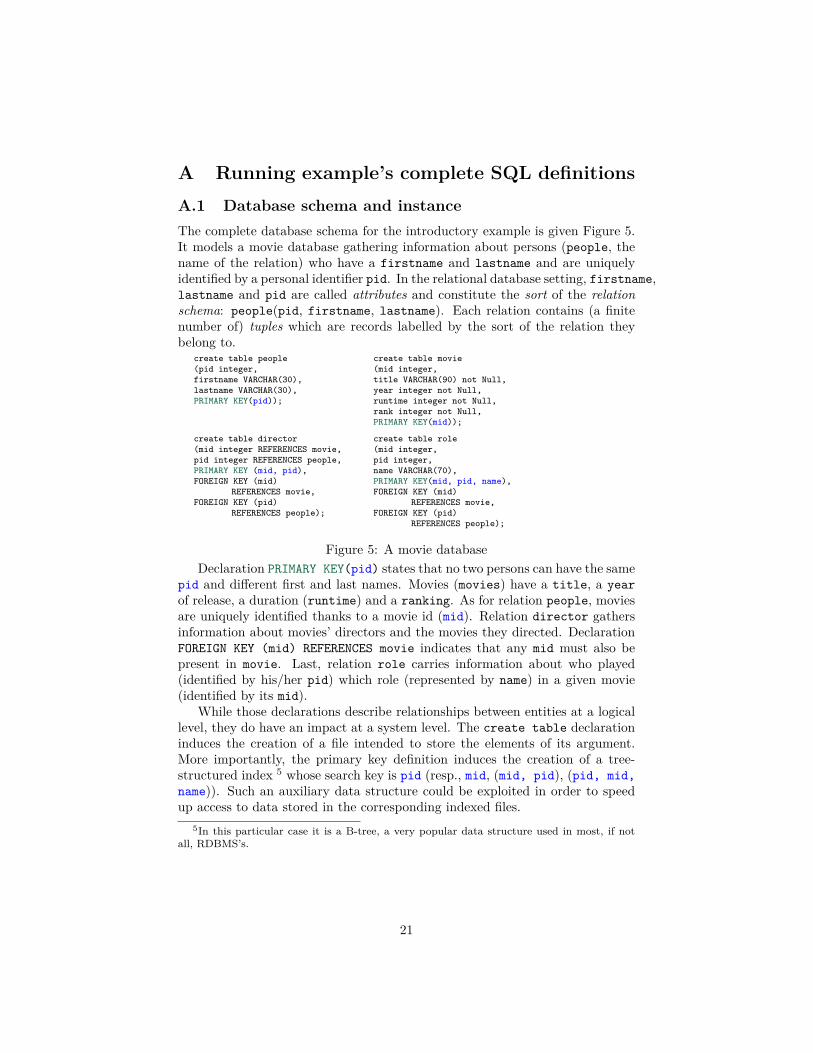
A Running example’s complete SQL definitionsA.1 Database schema and instanceThe complete database schema for the introductory example is given Figure 5.It models a movie database gathering information about persons (people, thename of the relation) who have a firstname and lastname and are uniquelyidentified by a personal identifier pid. In the relational database setting, firstname,lastname and pid are called attributes and constitute the sort of the relationschema: people(pid, firstname, lastname). Each relation contains (a finitenumber of) tuples which are records labelled by the sort of the relation theybelong to.

create table people(pid integer,firstname VARCHAR(30),lastname VARCHAR(30),PRIMARY KEY(pid));

create table movie(mid integer,title VARCHAR(90) not Null,year integer not Null,runtime integer not Null,rank integer not Null,PRIMARY KEY(mid));

create table director(mid integer REFERENCES movie,pid integer REFERENCES people,PRIMARY KEY (mid, pid),FOREIGN KEY (mid)

REFERENCES movie,FOREIGN KEY (pid)

REFERENCES people);

create table role(mid integer,pid integer,name VARCHAR(70),PRIMARY KEY(mid, pid, name),FOREIGN KEY (mid)

REFERENCES movie,FOREIGN KEY (pid)

REFERENCES people);

Figure 5: A movie databaseDeclaration PRIMARY KEY(pid) states that no two persons can have the same

pid and different first and last names. Movies (movies) have a title, a yearof release, a duration (runtime) and a ranking. As for relation people, moviesare uniquely identified thanks to a movie id (mid). Relation director gathersinformation about movies’ directors and the movies they directed. DeclarationFOREIGN KEY (mid) REFERENCES movie indicates that any mid must also bepresent in movie. Last, relation role carries information about who played(identified by his/her pid) which role (represented by name) in a given movie(identified by its mid).

While those declarations describe relationships between entities at a logicallevel, they do have an impact at a system level. The create table declarationinduces the creation of a file intended to store the elements of its argument.More importantly, the primary key definition induces the creation of a tree-structured index 5 whose search key is pid (resp., mid, (mid, pid), (pid, mid,name)). Such an auxiliary data structure could be exploited in order to speedup access to data stored in the corresponding indexed files.

5In this particular case it is a B-tree, a very popular data structure used in most, if notall, RDBMS’s.

21

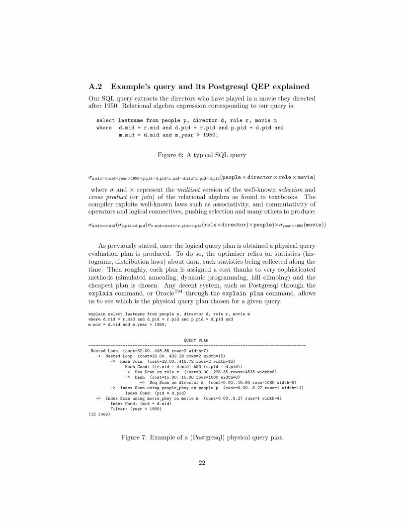
A.2 Example’s query and its Postgresql QEP explainedOur SQL query extracts the directors who have played in a movie they directedafter 1950. Relational algebra expression corresponding to our query is:

select lastname from people p, director d, role r, movie mwhere d.mid = r.mid and d.pid = r.pid and p.pid = d.pid and

m.mid = d.mid and m.year > 1950;

Figure 6: A typical SQL query

σm.mid=d.mid∧year>1950∧p.pid=d.pid∧r.mid=d.mid∧r.pid=d.pid(people×director×role×movie)

where σ and × represent the multiset version of the well-known selection andcross product (or join) of the relational algebra as found in textbooks. Thecompiler exploits well-known laws such as associativity, and commutativity ofoperators and logical connectives, pushing selection and many others to produce:

σm.mid=d.mid(σp.pid=d.pid(σr.mid=d.mid∧r.pid=d.pid(role×director)×people)×σyear>1950(movie))

As previously stated, once the logical query plan is obtained a physical queryevaluation plan is produced. To do so, the optimiser relies on statistics (his-tograms, distribution laws) about data, such statistics being collected along thetime. Then roughly, each plan is assigned a cost thanks to very sophisticatedmethods (simulated annealing, dynamic programming, hill climbing) and thecheapest plan is chosen. Any decent system, such as Postgresql through theexplain command, or OracleTM through the explain plan command, allowsus to see which is the physical query plan chosen for a given query.

explain select lastname from people p, director d, role r, movie mwhere d.mid = r.mid and d.pid = r.pid and p.pid = d.pid andm.mid = d.mid and m.year > 1950;

QUERY PLAN-----------------------------------------------------------------------------------------Nested Loop (cost=32.00..448.85 rows=2 width=7)

-> Nested Loop (cost=32.00..432.28 rows=2 width=15)-> Hash Join (cost=32.00..415.72 rows=2 width=16)

Hash Cond: ((r.mid = d.mid) AND (r.pid = d.pid))-> Seq Scan on role r (cost=0.00..238.35 rows=14535 width=8)-> Hash (cost=15.80..15.80 rows=1080 width=8)

-> Seq Scan on director d (cost=0.00..15.80 rows=1080 width=8)-> Index Scan using people_pkey on people p (cost=0.00..8.27 rows=1 width=11)

Index Cond: (pid = d.pid)-> Index Scan using movie_pkey on movie m (cost=0.00..8.27 rows=1 width=4)

Index Cond: (mid = d.mid)Filter: (year > 1950)

(12 rows)

Figure 7: Example of a (Postgresql) physical query plan

22

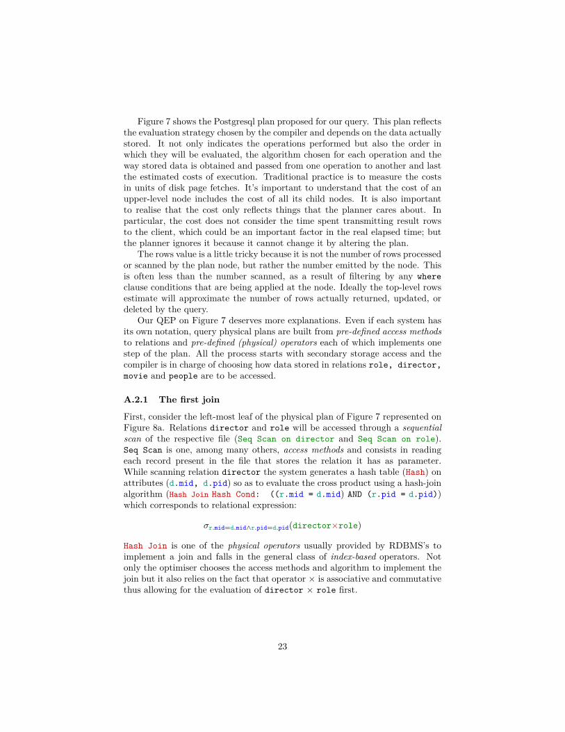
Figure 7 shows the Postgresql plan proposed for our query. This plan reflectsthe evaluation strategy chosen by the compiler and depends on the data actuallystored. It not only indicates the operations performed but also the order inwhich they will be evaluated, the algorithm chosen for each operation and theway stored data is obtained and passed from one operation to another and lastthe estimated costs of execution. Traditional practice is to measure the costsin units of disk page fetches. It’s important to understand that the cost of anupper-level node includes the cost of all its child nodes. It is also importantto realise that the cost only reflects things that the planner cares about. Inparticular, the cost does not consider the time spent transmitting result rowsto the client, which could be an important factor in the real elapsed time; butthe planner ignores it because it cannot change it by altering the plan.

The rows value is a little tricky because it is not the number of rows processedor scanned by the plan node, but rather the number emitted by the node. Thisis often less than the number scanned, as a result of filtering by any whereclause conditions that are being applied at the node. Ideally the top-level rowsestimate will approximate the number of rows actually returned, updated, ordeleted by the query.

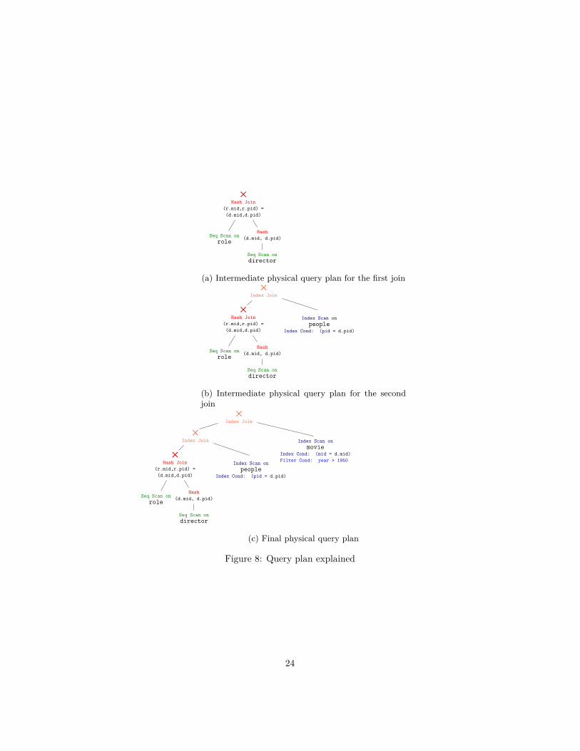
Our QEP on Figure 7 deserves more explanations. Even if each system hasits own notation, query physical plans are built from pre-defined access methodsto relations and pre-defined (physical) operators each of which implements onestep of the plan. All the process starts with secondary storage access and thecompiler is in charge of choosing how data stored in relations role, director,movie and people are to be accessed.

A.2.1 The first join

First, consider the left-most leaf of the physical plan of Figure 7 represented onFigure 8a. Relations director and role will be accessed through a sequentialscan of the respective file (Seq Scan on director and Seq Scan on role).Seq Scan is one, among many others, access methods and consists in readingeach record present in the file that stores the relation it has as parameter.While scanning relation director the system generates a hash table (Hash) onattributes (d.mid, d.pid) so as to evaluate the cross product using a hash-joinalgorithm (Hash Join Hash Cond: ((r.mid = d.mid) AND (r.pid = d.pid))which corresponds to relational expression:

σr.mid=d.mid∧r.pid=d.pid(director×role)

Hash Join is one of the physical operators usually provided by RDBMS’s toimplement a join and falls in the general class of index-based operators. Notonly the optimiser chooses the access methods and algorithm to implement thejoin but it also relies on the fact that operator × is associative and commutativethus allowing for the evaluation of director × role first.

23

5Hash Join

(r.mid,r.pid) =

(d.mid,d.pid)

Seq Scan on

role

Hash

(d.mid, d.pid)

Seq Scan on

director

(a) Intermediate physical query plan for the first join5

Index Join

5Hash Join

(r.mid,r.pid) =

(d.mid,d.pid)

Index Scan on

peopleIndex Cond: (pid = d.pid)

Seq Scan on

role

Hash

(d.mid, d.pid)

Seq Scan on

director

(b) Intermediate physical query plan for the secondjoin

5Index Join

5Index Join Index Scan on

movieIndex Cond: (mid = d.mid)

Filter Cond: year > 19505

Hash Join

(r.mid,r.pid) =

(d.mid,d.pid)

Index Scan on

peopleIndex Cond: (pid = d.pid)

Seq Scan on

role

Hash

(d.mid, d.pid)

Seq Scan on

director

(c) Final physical query plan

Figure 8: Query plan explained

24

A.2.2 The second join

Then, tuples resulting of the evaluation of the Hash Join are planned to bepassed on the fly to the upper operator, which is dependent on the evaluation ofthe first join. In particular each d.pid will serve as a constant and the index onrelation people whose search key is pid will be exploited to access people ele-ments by means of an index scan (Index Scan using people pkey on peoplep) with the (index) search condition Index Cond: (pid = d.pid). Indeed,the compiler does exploit the knowledge that an index, named people pkey, onrelation people whose search key is pid is available. The cross product betweenboth collections is achieved using the nested loop physical operator join algo-rithm (Nested Loop on the postgresql plan) combined with the Index Scan onpeople. The combination of both physical operators implements an index basedjoin (IndexJoin) (see Figure 8b) which corresponds to relational expression:

σp.pid=d.pid(σr.mid = d.mid∧

r.pid = d.pid

(director×role)×people)

A.2.3 The third join

Last movie’s elements are to be accessed exploiting the index (Index Scan usingmovie pkey on movie m Index Cond: (mid = d.mid)) and at the same time ele-ments that do not satisfy the filtering condition Filter: (year > 1950) will bediscarded. The combination of the corresponding elements is performed againthrough a nested loop algorithm (Nested Loop) yielding physical and logicalplans of Figure 8c. We would like to stress that, the computation, again, de-pends on the previously computed value d.mid. A last subtle point worth to bementionned is that rather than implementing:

σm.mid=d.mid(σp.pid=d.pid(σr.mid=d.mid∧r.pid=d.pid(role×director)×people)×σyear>1950(movie))

the plan implements rather

σm.mid=d.mid∧year>1950(σp.pid=d.pid(σr.mid=d.mid∧r.pid=d.pid(role×director)×people)×movie)

B Adequacy and bridge lemmas for Filter op-erators

Let us now explain how we use our high level specification in order to showthat the algebraic operator Q– Sigma is implemented by some physical operators,namely the simple Filter and IndexScan when the selection condition can be ex-pressed thank to an equality between index keys, keys being usually a list ofvalues taken by some attributes of the tuples.

First, assuming that we have a cursor c which contains elements of type A, wecan filter its content w.r.t theta by using Filter, provided that theta is compatiblew.r.t. the equivalence defined by the decidable comparison function in OA.

25

Section Filter– is– a– filter– op.Hypothesis A : Type.Hypothesis OA : Oeset.Rcd A.Hypothesis C : Cursor.Rcd OA.Hypothesis theta : A → bool.Hypothesis theta– eq : ∀ x1 x2, Oeset.compare OA x1 x2 = Eq → theta x1 = theta x2.

Lemma mk– filter– is– a– filter– op :let F := (Filter.build – theta– eq C) inis– a– filter– op(∗ a record containing a deciable comparison function over the elements to be selected ∗)

OA(∗ how to retrieve the elements to be selected from the input container ∗)

(Cursor.materialize C)(∗ how to retrieve the selected elements from the output container ∗)

(Cursor.materialize F)(∗ selection condition ∗)

theta(∗ the actual filter, which produced the output container from the input container ∗)

(Filter.mk– filter F).End Filter– is– a– filter– op.

Section IndexScan– is– a– filter– op.Variable o1 o2 : Type.Variable O1 : Oeset.Rcd o1.Variable O2 : Oeset.Rcd o2.Variable IS : Index.Rcd O1 O2.

Lemma IS– is– a– filter– op :∀ (x1 : o1),is– a– filter– op(∗ a record containing a deciable comparison function over the elements to be selected ∗)

O1(∗ how to retrieve the elements to be selected from the input container ∗)

(Index.c1 IS)(∗ how to retrieve the selected elements from the output container ∗)

(Cursor.materialize (Index.C1 IS))(∗ selection condition: having the same key as [o1] ∗)

(fun x ⇒ Index.P IS (Index.proj IS x1) (Index.proj IS x))(∗ the actual filter, which produced the output container from the input container ∗)

(fun c ⇒ Index.i IS c (Index.proj IS x1)).End IndexScan– is– a– filter– op.

Assuming that all needed ingredients (tuples with a decidable comparison,functions, predicates, aggregates with their respectives interpretations, etc.)are present to define the evaluation of an algebraic query, Q– Sigma is alsois– a– filter– op:Lemma Q– Sigma– is– a– filter– op :∀ env f,

is– a– filter– op(∗ a record containing a deciable comparison function over the elements to be selected ∗)

26

(OTuple T)(∗ how to retrieve the elements to be selected from the input container ∗)

(fun q ⇒Febag.elements BTupleT (eval– query env q))(∗ how to retrieve the selected elements from the output container ∗)

(fun q ⇒Febag.elements BTupleT (eval– query env q))(∗ selection condition: satisfying the formula [f] ∗)

(fun t ⇒ eval– formula (env– t env t) f)(∗ the actual filter, which produced the output container from the input container ∗)

(fun q ⇒Q– Sigma f q).It is now easy to bridge the above lemmas to show that fun q ⇒Q– Sigma f q

can always be implemented by a simple Filter built over a cursor which imple-ments the algebraic query q and using as a filtering condition the evaluation ofthe formula f.Notation ”b ’=R=’ l” :=

(∀ t, Febag.nb– occ BTupleT t b = Oeset.nb– occ (OTuple T) t l) (at level 70, no associativity).Lemma mk– filter– implements– Q– Sigma :∀C env f q,

let F := Filter.build – (eval– f– eq env f) C in∀ c,

eval– query env q =R= Cursor.materialize C c →eval– query env (Q– Sigma f q) =R= Cursor.materialize F (Filter.mk– filter F c).

When the formula f has the special form of a conjunction of equalities forthe values taken by some attributes, as in our example , it is also possible touse an IndexScan:Lemma IS– implements– Q– Sigma :∀ (∗ the keys of the index are lists of values ∗)

(IS : Index.Rcd (OTuple T) (oeset– of– oset (mk– olists (OVal T)))),(∗ the condition used to build the index is actually the equality of these lists of values ∗)(∀ lv1 lv2, Index.P IS lv1 lv2 = Oset.eq– bool (mk– olists (OVal T)) lv1 lv2) →∀ la lval env f q ,(∗ the selection formula of the algebraic query corresponds to the equality between a key [lval]

and the dot extraction over a given list of attributes [la] ∗)(∀ t, eval– formula (env– t env t) f =

Oset.eq– bool (mk– olists (OVal T)) (map (dot T t) la) lval) →(∗ the projection used to build the index is actually the dot extraction over [la] ∗)(∀ t, Index.proj IS t = map (dot T t) la) →∀ c,

eval– query env q =R= Index.c1 IS c →eval– query env (Q– Sigma f q) =R= Cursor.materialize – (Index.i IS c lval).

The same kind of arguments hold for the other operators and are detailed inthe accompanying development at http://datacert.lri.fr/sqlcert/itp18.tar.gz.

C Proof of concept: the example QEPWe have all the ingredients to design a language for query execution plans, thatis interpreted using our cursors and indices from Section 4. We focus in thisappendix on its subset applied to the example of Fig. 1.

27

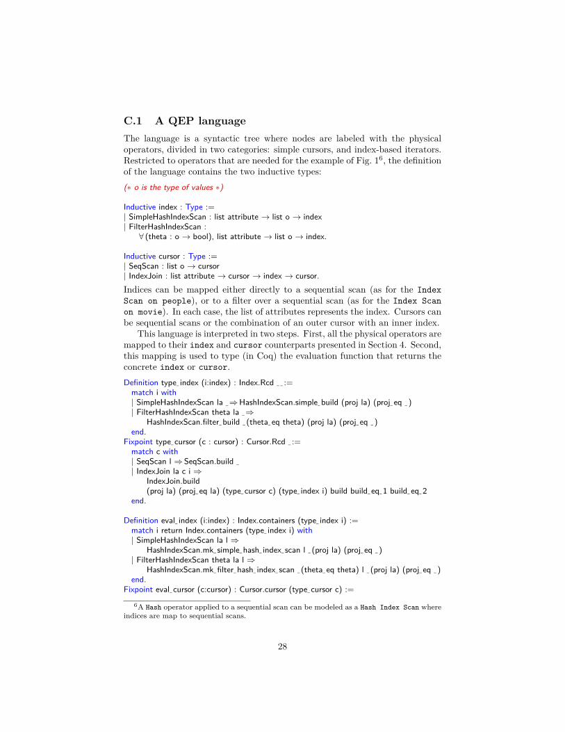
C.1 A QEP languageThe language is a syntactic tree where nodes are labeled with the physicaloperators, divided in two categories: simple cursors, and index-based iterators.Restricted to operators that are needed for the example of Fig. 16, the definitionof the language contains the two inductive types:(∗ o is the type of values ∗)

Inductive index : Type :=| SimpleHashIndexScan : list attribute → list o → index| FilterHashIndexScan :∀ (theta : o → bool), list attribute → list o → index.

Inductive cursor : Type :=| SeqScan : list o → cursor| IndexJoin : list attribute → cursor → index → cursor.Indices can be mapped either directly to a sequential scan (as for the IndexScan on people), or to a filter over a sequential scan (as for the Index Scanon movie). In each case, the list of attributes represents the index. Cursors canbe sequential scans or the combination of an outer cursor with an inner index.

This language is interpreted in two steps. First, all the physical operators aremapped to their index and cursor counterparts presented in Section 4. Second,this mapping is used to type (in Coq) the evaluation function that returns theconcrete index or cursor.Definition type– index (i:index) : Index.Rcd – – :=

match i with| SimpleHashIndexScan la –⇒HashIndexScan.simple– build (proj la) (proj– eq – )| FilterHashIndexScan theta la –⇒

HashIndexScan.filter– build – (theta– eq theta) (proj la) (proj– eq – )end.

Fixpoint type– cursor (c : cursor) : Cursor.Rcd – :=match c with| SeqScan l ⇒SeqScan.build –

| IndexJoin la c i ⇒IndexJoin.build(proj la) (proj– eq la) (type– cursor c) (type– index i) build build– eq– 1 build– eq– 2

end.

Definition eval– index (i:index) : Index.containers (type– index i) :=match i return Index.containers (type– index i) with| SimpleHashIndexScan la l ⇒

HashIndexScan.mk– simple– hash– index– scan l – (proj la) (proj– eq – )| FilterHashIndexScan theta la l ⇒

HashIndexScan.mk– filter– hash– index– scan – (theta– eq theta) l – (proj la) (proj– eq – )end.

Fixpoint eval– cursor (c:cursor) : Cursor.cursor (type– cursor c) :=

6A Hash operator applied to a sequential scan can be modeled as a Hash Index Scan whereindices are map to sequential scans.

28

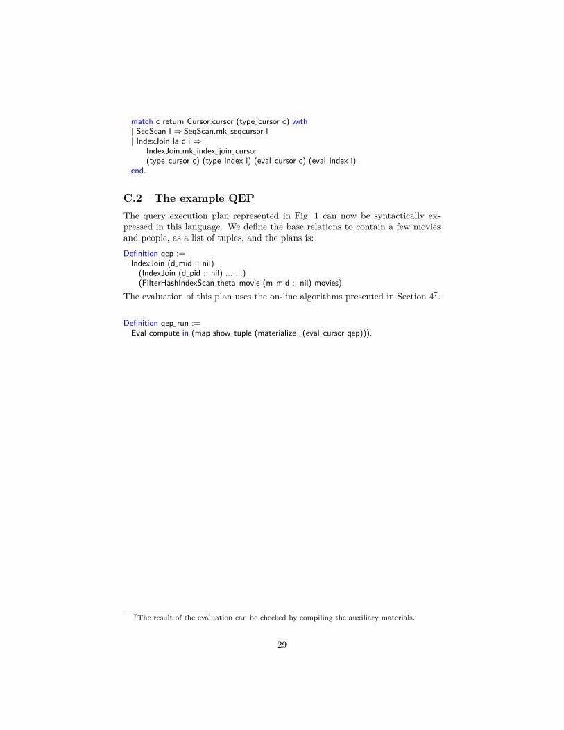
match c return Cursor.cursor (type– cursor c) with| SeqScan l ⇒SeqScan.mk– seqcursor l| IndexJoin la c i ⇒

IndexJoin.mk– index– join– cursor(type– cursor c) (type– index i) (eval– cursor c) (eval– index i)

end.

C.2 The example QEPThe query execution plan represented in Fig. 1 can now be syntactically ex-pressed in this language. We define the base relations to contain a few moviesand people, as a list of tuples, and the plans is:Definition qep :=

IndexJoin (d– mid :: nil)(IndexJoin (d– pid :: nil) ... ...)(FilterHashIndexScan theta– movie (m– mid :: nil) movies).

The evaluation of this plan uses the on-line algorithms presented in Section 47.

Definition qep– run :=Eval compute in (map show– tuple (materialize – (eval– cursor qep))).

7The result of the evaluation can be checked by compiling the auxiliary materials.

29