A coordination methodology for radionavigation-satellite ... · Recommendation ITU-R M.1831-1...

Recommendation ITU-R M.1831-1 (09/2015)

A coordination methodology for radionavigation-satellite service

inter-system interference estimation

M Series

Mobile, radiodetermination, amateur

and related satellite services

ii Rec. ITU-R M.1831-1

Foreword

The role of the Radiocommunication Sector is to ensure the rational, equitable, efficient and economical use of the radio-

frequency spectrum by all radiocommunication services, including satellite services, and carry out studies without limit

of frequency range on the basis of which Recommendations are adopted.

The regulatory and policy functions of the Radiocommunication Sector are performed by World and Regional

Radiocommunication Conferences and Radiocommunication Assemblies supported by Study Groups.

Policy on Intellectual Property Right (IPR)

ITU-R policy on IPR is described in the Common Patent Policy for ITU-T/ITU-R/ISO/IEC referenced in Annex 1 of

Resolution ITU-R 1. Forms to be used for the submission of patent statements and licensing declarations by patent holders

are available from http://www.itu.int/ITU-R/go/patents/en where the Guidelines for Implementation of the Common

Patent Policy for ITU-T/ITU-R/ISO/IEC and the ITU-R patent information database can also be found.

Series of ITU-R Recommendations

(Also available online at http://www.itu.int/publ/R-REC/en)

Series Title

BO Satellite delivery

BR Recording for production, archival and play-out; film for television

BS Broadcasting service (sound)

BT Broadcasting service (television)

F Fixed service

M Mobile, radiodetermination, amateur and related satellite services

P Radiowave propagation

RA Radio astronomy

RS Remote sensing systems

S Fixed-satellite service

SA Space applications and meteorology

SF Frequency sharing and coordination between fixed-satellite and fixed service systems

SM Spectrum management

SNG Satellite news gathering

TF Time signals and frequency standards emissions

V Vocabulary and related subjects

Note: This ITU-R Recommendation was approved in English under the procedure detailed in Resolution ITU-R

1.

Electronic Publication

Geneva, 2015

ITU 2015

All rights reserved. No part of this publication may be reproduced, by any means whatsoever, without written permission of ITU.

http://www.itu.int/ITU-R/go/patents/en

http://www.itu.int/publ/R-REC/en

Rec. ITU-R M.1831-1 1

RECOMMENDATION ITU-R M.1831-1

A coordination methodology for radionavigation-satellite service

inter-system interference estimation

(Question ITU-R 217-2/4)

(2007-2015)

Scope

This Recommendation gives a methodology for radionavigation-satellite service (RNSS) intersystem

interference estimation to be used in coordination between systems and networks in the RNSS. As

Resolution 610 (WRC-03) applies to all systems and networks in the RNSS and contains measures that are

designed to facilitate RNSS inter-system compatibility determination, this Recommendation is applicable to

the RNSS in the bands 1 164-1 215 MHz, 1 215-1 300 MHz, 1 559-1 610 MHz and 5 010-5 030 MHz.

Keywords

RNSS, coordination methodology, intersystem interference estimation

Abbreviations/Glossary

ADC Analogue-to-Digital Converter

AGC Automatic Gain Control

PRN Pseudo-Random Noise

SSC Spectral Separation Coefficient

Related ITU Recommendations, Reports

Recommendation ITU-R M.1318-1 Evaluation model for continuous interference from radio

sources other than in the radionavigation-satellite service to the

radionavigation-satellite service systems and networks

operating in the 1 164-1 215 MHz, 1 215-1 300 MHz,

1 559-1 610 MHz and 5 010-5 030 MHz bands

Recommendation ITU-R M.1787-2 Description of systems and networks in the radionavigation-

satellite service (space-to-Earth and space-to-space) and

technical characteristics of transmitting space stations

operating in the bands 1 164-1 215 MHz,1 215-1 300 MHz and

1 559-1 610 MHz

Recommendation ITU-R M.1901-1 Guidance on ITU-R Recommendations related to systems and

networks in the radionavigation-satellite service operating in

the frequency bands 1 164-1 215 MHz, 1 215-1 300 MHz,

1 559-1 610 MHz, 5 000-5 010 MHz and 5 010-5 030 MHz

Recommendation ITU-R M.1902-0 Characteristics and protection criteria for receiving earth

stations in the radionavigation-satellite service

(space-to-Earth) operating in the band 1 215-1 300 MHz



(space-to-Earth) and receivers in the aeronautical

radionavigation service operating in the band 1 559-1 610 MHz

2 Rec. ITU-R M.1831-1

Recommendation ITU-R M.1904-0 Characteristics, performance requirements and protection

criteria for receiving stations of the radionavigation-satellite

service (space-to-space) operating in the frequency bands

1 164-1 215 MHz, 1 215-1 300 MHz and 1 559-1 610 MHz



(space-to-Earth) operating in the band 1 164-1 215 MHz

Recommendation ITU-R M.1906-1 Characteristics and protection criteria of receiving space

stations and characteristics of transmitting earth stations in the

radionavigation-satellite service (Earth-to-space) operating in

the band 5 000-5 010 MHz

Recommendation ITU-R M.2030-0 Evaluation method for pulsed interference from relevant radio

sources other than in the radionavigation-satellite service to the

radionavigation-satellite service systems and networks

operating in the 1 164-1 215 MHz, 1 215-1 300 MHz and

1 559-1 610 MHz frequency bands

Recommendation ITU-R M.2031-1 Characteristics and protection criteria of receiving earth

stations and characteristics of transmitting space stations of the

radionavigation-satellite service (space-to-Earth) operating in

the band 5 010-5 030 MHz

The ITU Radiocommunication Assembly,

considering

a) that systems and networks in the radionavigation-satellite service (RNSS) provide worldwide

accurate information for many positioning and timing applications including critical ones related to

safety of life;

b) that WRC-03 adopted new and expanded allocations for the RNSS;

c) that any properly equipped earth station may receive navigation information from systems

and networks in the RNSS on a worldwide basis;

d) that there are several operating and planned systems and networks in the RNSS and an

increasing number of RNSS filings at the Radiocommunication Bureau proposing to use the RNSS

allocations;

e) that methods have been developed for use in coordination discussions which provide

a common basis for the estimation of interference between such systems and networks in the RNSS,

recognizing

a) that the bands 1 164-1 215 MHz, 1 215-1 300 MHz, 1 559-1 610 MHz and 5 010-5 030 MHz

are allocated on a primary basis to RNSS (space-to-Earth, space-to-space);

b) that the bands 1 164-1 215 MHz, 1 215-1 300 MHz, 1 559-1 610 MHz and

5 010-5 030 MHz are also allocated on a primary basis to other services;

c) that Recommendation ITU-R M.1901 provides guidance on this and other ITU-R

Recommendations related to systems and networks in the RNSS operating in the frequency bands

1 164-1 215 MHz, 1 215-1 300 MHz, 1 559-1 610 MHz, 5 000-5 010 MHz and 5 010-5 030 MHz;

Rec. ITU-R M.1831-1 3

d) that technical and operational characteristics of, and protection criteria for, system and

network receivers in the RNSS (space-to-Earth and space-to-space) in the bands 1 164-1 215 MHz,

1 215-1 300 MHz, 1 559-1 610 MHz, 5 000-5 010 MHz and 5 010-5 030 MHz are provided in

Recommendations ITU-R M.1905, ITU-R M.1902, ITU-R M.1903, ITU-R M.1904, ITU-R M.1906

and ITU-R M.2031;

e) that technical and operational characteristics of system and network transmitters in the RNSS

(Earth-to-space, space-to-Earth and space-to-space) in the bands 1 164-1 215 MHz,

1 215-1 300 MHz, 1 559-1 610 MHz, 5 000-5 010 MHz and 5 010-5 030 MHz are provided in

Recommendations ITU-R M.1787, ITU-R M.1906 and ITU-R M.2031;

f) that Recommendation ITU-R M.1318 provides a model for evaluating interference from

environmental sources into RNSS systems in the bands 1 164-1 215 MHz, 1 215-1 300 MHz,

1 559-1 610 MHz and 5 010-5 030 MHz;

g) that Recommendation ITU-R M.2030 provides an evaluation method for pulsed interference

from relevant radio sources other than in the RNSS to the RNSS systems and networks operating in

the 1 164-1 215 MHz, 1 215-1 300 MHz and 1 559-1 610 MHz bands;

h) that No. 4.10 of the Radio Regulations (RR) states that the safety aspects of RNSS “require

special measures to ensure their freedom from harmful interference”;

i) that under RR No. 5.328B systems and networks in the RNSS intending to use the bands

1 164-1 215 MHz, 1 215-1 300 MHz, 1 559-1 610 MHz and 5 010-5 030 MHz for which complete

coordination or notification information, as appropriate, is received by the Radiocommunication

Bureau after 1 January 2005 are subject to the application of the provisions of RR Nos. 9.12, 9.12A

and 9.13, and studies to determine additional methodologies and criteria to facilitate such

coordination are being planned;

j) that under RR No. 9.7, stations in RNSS networks using the geostationary-satellite orbit are

subject to coordination with other such stations, and studies to determine additional methodologies

and criteria to facilitate such coordination are being planned,

further recognizing

that Resolution 610 (WRC-03) applies to all systems and networks in the RNSS in the bands

mentioned in recognizing a), and contains measures that are designed to facilitate the making of RNSS

inter-system compatibility determinations,

recommends

1 that the methodology in Annex 1 should be used in carrying out coordination between RNSS

systems operating or proposed to operate in one or more of the same frequency bands identified in

recognizing a) (see Note 1);

2 that the guidance in Annexes 2 and 3 should be taken into account by RNSS system operators

before and during RNSS coordination.

NOTE 1 – The methodology in Annex 1 may be difficult to apply to multi-satellite FDMA RNSS

systems. In this case, Annex 2 may be implemented.

4 Rec. ITU-R M.1831-1

Annex 1

A method for estimating inter-system interference between

systems and networks in the RNSS

TABLE OF CONTENTS

Page

1 Introduction .................................................................................................................... 5

2 Interference analysis methodology ................................................................................. 5

3 Data used in the calculations .......................................................................................... 8

3.1 Constellation and satellite transmitter models .................................................... 8

3.2 User receiver model ............................................................................................ 9

3.3 Interference and noise model .............................................................................. 9

4 A simulation-based approach for calculating Gagg ......................................................... 10

5 A hypothetical example of the methodology’s application ............................................ 14

5.1 An assessment of interference levels .................................................................. 14

5.2 An assessment of effective carrier-to-noise ratios and related degradation ....... 16

6 RNSS short-code spectrum characteristics and modelling ............................................. 18

6.1 RNSS short-PRN code spectrum example ......................................................... 18

6.2 General aspects of detailed dynamic modelling for RNSS short PRN codes ..... 19

7 Conclusion ...................................................................................................................... 20

Rec. ITU-R M.1831-1 5

1 Introduction

This methodology is intended to provide a technique of estimating the interference between systems

and networks in the RNSS. As such, it is useful for inter-system RNSS coordination. (For the purpose

of brevity, the word “system” will be used instead of “system or network” in the remainder of this

document.) The methodology applies to RNSS systems that use CDMA and FDMA to allow sharing

of RNSS bands, and recognizes that a simple summation of transmission power density is inadequate

to determine what effect an RNSS system will have on others. Unlike RNSS CDMA systems, which

typically have only one carrier per occupied band, FDMA systems have several carriers in a single

occupied band. It may not be practical to apply the methodology below to each carrier frequency used

in a multi-satellite FDMA system.

2 Interference analysis methodology

Typically, the post-correlator effective carrier-to-noise density ratio, 0/ NC , is used to measure the

impact of the interference from various sources on the operational performance of the intended

receivers. 0/ NC is dependent on the receiver, antenna and external noise from non-RNSS sources.

However, it is used in assessing inter-system interference of RNSS systems.

For the case of continuous interference1, 0/ NC is given by:

extintref IIIN

C

N

C

00

(1)

where:

C: post-correlator received desired-signal power (W) from the satellite in the

reference constellation including any relevant processing losses2

N0: receiver pre-correlator thermal noise power spectral density (W/Hz)

N'0: post-correlator effective receiver thermal noise power spectral density (W/Hz)

Iref: post-correlator effective white-noise power spectral-density (W/Hz) due to the

aggregate interference from all the signals, except the desired signal, transmitted

by all the in-view satellites in the reference constellation including any relevant

processing losses

Iint: post-correlator effective white-noise power spectral-density (W/Hz) due to the

aggregate interference from all the signals transmitted in the frequency band of

interest by all the in-view RNSS satellites other than those in the reference

constellation, including any relevant processing losses

Iext: post-correlator effective white-noise power spectral-density (W/Hz) due to the

aggregate interference from all radio signals other than those of the RNSS,

including any relevant processing losses

: dimensionless effective thermal noise factor given by:

1 When significant pulsed interference is present, equation (1) must be modified. Pulsed interference reduces

signal-to-noise ratio by suppressing the desired signal and increasing the effective noise floor.

2 Relevant processing losses include transmitter and receiver antenna gains; receiver implementation loss,

such as filtering and quantization losses; and mismatch losses between the received signal and the reference

code.

6 Rec. ITU-R M.1831-1

ffSfH d)()(2

)( fH : normalized equivalent transfer function, at frequency f (Hz) given by:

H

fHfH

max

H(f): equivalent receiver filter transfer function (dimensionless), at frequency f (Hz),

representing all of the pre-correlator receiver front-end filtering

S(f): ideal equivalent two-sided power spectral density (W/Hz), at frequency f (Hz) of

the unfiltered pre-correlator desired signal, normalized to unit power over an

infinite bandwidth, and is computed assuming random spreading codes

: dummy variable.

The receiver’s effective post-correlator thermal noise level, in the absence of external noise, reduces

to 00 vNN . In addition, if H represents an ideal bandpass filter with bandwidth BR (rather than the

detailed magnitude transfer function of the receiver’s front-end filter), then simplifies to:

1d)(d)(

2/

2/

ffSffSR

R

B

B

It should be noted that Iint (W/Hz) can be further broken down to consider the interference due to a

specific RNSS system:

Iint Ialt Irem

where:

Ialt: post-correlator effective noise power spectral-density (W/Hz) due to the


interest by all the in-view satellites of a specific “alternate” constellation

Irem: post-correlator effective noise power spectral-density (W/Hz) due to the


interest by all the in-view “remaining” RNSS satellites; i.e. those that are not in

either the reference constellation or the alternate constellation.

To calculate the effective noise power spectral densities we define the spectral separation coefficient,

β (in units of 1/Hz), of an interfering signal from the n-th signal of the m-th satellite to a desired

signal, x, as:

ffSfSfH nmx

x

nm

d)()()( ,

2

,

(2)

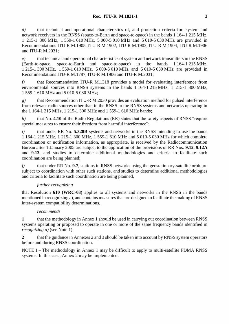
where:

)( fS x : normalized (to unity over the transmission bandwidth) two-sided power spectral

density (W/Hz), at frequency f (Hz) of the desired signal:

Rec. ITU-R M.1831-1 7

elsewhere0

2/

dγ)γ(

)(

)(

2/

2/

TDB

B

x

x

x

Bf

S

fS

fSTD

TD

BTD: transmission bandwidth (Hz) over which the desired signal’s power is defined

Sx(f): two-sided power spectral density (W/Hz), at frequency f (Hz) of the unfiltered

desired signal

, ( )m nS f: normalized (to unity over the transmission bandwidth) two-sided power spectral

density (W/Hz), at frequency f (Hz) of the n-th interfering signal from the m-th

satellite in a constellation:

elsewhere0

2/

dγ)γ(

)(

)(

2/

2/

,

,

,

TB

B

nm

nm

nm

Bf

S

fS

fST

T

and

, ( )m nS f: two-sided power spectral density (W/Hz) at frequency f (Hz) of the unfiltered

n-th interfering signal from the m-th satellite in a constellation

BT: transmission bandwidth (Hz) over which the interfering signal’s power is

defined.

Equation (2) implicitly assumes that the PRN (pseudo-random noise) code modulated RNSS signals,

represented by S, can be approximated as a continuous spectrum in the aggregate interference

spectrum. This may not be true for certain signals with “short” PRN codes. Further explanation is

provided in § 6.

Let:

Mref: number of visible satellites in the reference satellite constellation

Nref,m: number of interfering signals (not including the desired signal from the desired

satellite) that is transmitted by the m-th satellite in the reference satellite

constellation

Malt: number of visible RNSS satellites in the alternate satellite constellation

Nalt,m: number of interfering signals transmitted by the m-th satellite in the alternate

satellite constellation (which can be assumed the same for all satellites in the

alternate constellation if an absent signal’s power is set to zero)

Mrem: number of visible RNSS satellites that are not in the reference or the alternate

satellite constellation

Nrem,m: number of interfering signals transmitted by the m-th satellite that is not in the

reference or alternate constellation

refnmP ,: maximum interfering power (W) of the n-th interfering signal on the m-th

satellite in the reference constellation

Lm,n

ref : (dimensionless) processing loss of the n-th interfering signal on the m-th satellite

in the reference constellation

alt

nmP , : maximum interfering power (W) of the n-th signal on the m-th satellite in the

alternate constellation

8 Rec. ITU-R M.1831-1

alt

nmL , : (dimensionless) processing loss of the n-th signal on the m-th satellite in the

alternate constellation

rem

nmP , : maximum interfering power (W) of the n-th signal on the m-th satellite in the

remaining RNSS constellations

rem

nmL , : be the (dimensionless) processing loss of the n-th signal on the m-th satellite in

the remaining RNSS constellations.

With these definitions we can write equations to calculate the effective interference power spectral

density to reception from the reference constellation, the alternate constellation, and the remaining

constellations as follows:

refM

mref

nm

refnm

xnm

mrefN

n

refL

PI

1 ,

,,,

1

(3)

altM

malt

nm

altnm

xnm

maltN

n

altL

PI

1 ,

,,,

1

(4)

remM

mrem

nm

remnm

xnm

mremN

n

remL

PI

1 ,

,,,

1

(5)

Using equations (1) to (5) the effective carrier-to-noise density ratio 0/ NC can be calculated.

This number can then be compared with a 0/ NC threshold based upon the receiver mode, code

acquisition, code tracking, carrier tracking and data demodulation, to measure the effect of

interference.

Other methodologies based on the effective carrier-to-noise ratio 0/ NC , including its degradation due

to a specific alternate constellation only, may be used. The degree of interoperability among signals,

or specific inter-system code cross-correlation properties, may also be taken into account. Examples

of the application of these measures are shown in § 5.2.

3 Data used in the calculations

The data used in the calculations will often be measured, determined by simulations, or adjusted to

produce results consistent with experience. In addition, calculation of these values for each satellite

and each signal is typically simulated over a period of time over an area of interest, and the statistics

of inter-system interference values can then be obtained for consideration.

The subsections below provide further comment on how input for the calculations may be obtained.

3.1 Constellation and satellite transmitter models

Dynamic constellation simulation models with the respective orbital parameters are used to determine

the received power levels for the desired and the interfering signals. A simplified satellite transmitter

model is shown in Fig. 1.

Rec. ITU-R M.1831-1 9

FIGURE 1

Simplified satellite transmitter model

M.1831-01

Transmit filter

Signalgeneration

Transmit antenna

3.1.1 Worst-case received signal levels

For the worst-case interference calculation the desired signal is taken at the minimum power and

the interfering signal is taken at the maximum power. This includes all RNSS signals in the reference

constellation except the desired signal.

3.1.2 Spectral separation coefficients ()

The values are calculated with an assumption for both the transmission and receiver bandwidths.

Note that the values computed using equation (2) could be lower than those experienced.

For example, this can occur for “short” PRN codes (see § 6). This is due to the relatively coarser

spectral-line structure of short PRN codes that may not be accurately represented by a continuous

power spectral-density function in equation (2).

3.2 User receiver model

The user receiver model is shown in Fig. 2. The receiver antenna, the output of which is input to the

receiver front-end filter, receives both the desired and the interfering signals. The automatic gain

control (AGC) loop keeps the voltage input to the analogue to digital converter (ADC) within the

dynamic range of the ADC. Correlation is performed using the received signal and a locally generated

signal matched to the transmitted signal prior to transmit filtering. All the losses namely, filtering,

ADC and the correlator mismatch losses are grouped into a single loss factor. However, losses for the

desired signal can be different than losses for interfering signals.

FIGURE 2

Simplified user receiver model

M.1831-02

Receiver front-end

filter

AGC and ADC

Correlator

Filter losses ADC losses Mismatch losses

Receive antenna

3.3 Interference and noise model

Navigation signal parameters are given in terms of data rate, PRN code chip rate and other code

characteristics and modulation types. A continuous spectrum approximation is used to model the

combined spectrum of the received interfering signals with the exception of short-period codes for

which the spectral line nature of the code is taken into account.

User location can also be taken into account by measuring the interference power at every location

on the earth over a 24-hour period. For a given type of interfering RNSS signal, that type’s maximum

aggregate interference level is calculated and compared to the maximum interfering power per

satellite of a single such interfering signal to yield an aggregate gain factor (Gagg). In other words,

10 Rec. ITU-R M.1831-1

Gagg takes the maximum power of a single signal of an RNSS signal type, and is the increase needed

to relate that power to the power of all interfering signals of that type. This factor thus accounts for

all other signals of the same type as well as the variation in antenna gain towards all satellites

transmitting that signal type.

In practice, a Gagg value can be computed for a given constellation for a single signal, as shown in § 4,

and then applied to all of that constellation’s signals, or it may be the subject of coordination

discussions. Similarly other interference values can also be simplified.

Interference from continuous external wideband sources is typically modelled as a noise source with

a constant equivalent noise power spectral-density value, Iext. This term is intended to account for all

radio sources outside of the RNSS, and it may include in-band or out-of-band interference from other

radio services.

Additional methods need to be defined for narrowband and pulsed interference.

4 A simulation-based approach for calculating Gagg

The post-correlator aggregate interference power spectral density to a desired signal, indexed by k,

from all the satellites within a RNSS system to a receiver at a given location, indexed by i, can be

written in terms of spectral separation coefficient, transmit power, transmit/receive antenna gain, path

loss, and processing loss as follows:

kk

kk

kk

Rk

Tk

N

n nk

nmk

nmmi

Rmi

Tmi

tM

m

kiL

PttGtG

L

PtGtGtI

mSi

,

,0,00,,0,0

1 ,

,,,,,

)(

0

, )()()()()()(

(6)

where:

i: receiver index

k: index of the desired signal type

t: time for which the aggregate interference power is being calculated

( )S

iM t: number of RNSS satellites in view at the i-th receiver’s location at time t

m: index of the summation over satellites in view and m = 0 for the desired signal’s

satellite index

,

T

i mG: (dimensionless) transmit-antenna gain (relative to isotropic) between the m-th

satellite to the i-th receiver location

,

R

i mG: (dimensionless) receive-antenna gain (relative to isotropic) between the i-th

receiver location and the m-th satellite

i,m: (dimensionless) path loss from the m-th satellite to the i-th receiver location;

Nm: total number of signal types on the m-th satellite

,

k

m n: spectral separation coefficient (1/Hz) between the k-th signal type and n-th signal

type of the m-th satellite

Pm,n: transmitted power (W) of the n-th signal on the m-th satellite

Lk,n: (dimensionless) processing loss for the n-th signal type (when the k-th signal

type is desired).

In equation (6), the first term is the sum of all power spectral densities from all satellites in view and

for all signals, including the desired signal from the desired satellite, while the second term is the

power spectral density of the desired signal from the desired satellite.

Rec. ITU-R M.1831-1 11

As can be seen from equation (6) the equivalent power spectral density causes the thermal noise floor

to go up. Ii,k(t) is a function of time, user location and the spectral separation coefficient.

A straightforward method to determine Ii,k(t) is to use constellation simulation software in each and

every interference scenario to determine the resulting amount of interference. It is too cumbersome

and time consuming to perform this calculation using constellation simulation every time and place

an interference analysis is needed. It is helpful to have a single factor that can be used repeatedly in

interference analyses without resorting to the use of constellation simulation for every scenario. This

factor can be derived using simulation models and thereby avoid the repeated computation of Ii,k(t).

This factor is called aggregate gain factor, Gagg, which can be obtained from taking an upper bound

on equation (6) using the worst-case scenario. This overstates the interference in most situations, but

it also provides confidence that the computed threshold interference level will not be exceeded.

The Gagg, for a particular signal type, can be derived as follows:

a) At each position, indexed by i, in space (but usually on or near the Earth’s surface) the

received interference power (W) at the i-th receiver position can be written as:

( )

, , ,

0

( ) ( ) ( ) ( )

SiM t

R T Ri i m i m i m m

m

P t G t G t t P

(7)

Note that in equation (7), for the sake of simplicity, the index referring to the desired signal type,

k, has been dropped and the processing losses, Lm, are accounted for elsewhere (cf. equation (9)).

If the desired and the interfering signals are of the same type, a minor adjustment in equation (7)

is necessary in which one should subtract the desired signal power from equation (7).

b) Now we can write, for each receiver position, the equation for Gagg (dimensionless) as:

Gagg =max

all imax

all tP

i

R(t)( )éë

ùû

Pmax

R (8)

Here RmaxP is the maximum signal-power (W) of the interference signal type under consideration from

any single satellite, at a reference receiver’s antenna output and before the receiver’s RF filter, taken

over all indexed receiver locations. Note that a reference receiving antenna (for a particular system)

can be an appropriate anisotropic antenna. Such an antenna may not be matched to the received signal

type in polarization, resulting in some additional attenuation. Gagg is computed from equation (8) for

all interfering signal types.

The resulting Gagg is the worst-case value over all the receiver positions used in its calculation.

This value is then used to represent the worst-case Gagg for any receiver positions used in the

interference analysis (for the desired signal type).

The power spectral density of interference from all RNSS signals from all RNSS satellites in view, I0

(W/Hz), can then be bounded above by:

N

n n

Rnmaxn

aggn

L

PGI

1

,0 (9)

where n is the spectral separation coefficient between the desired signal and the n-th signal-type and

Ln is the processing loss between the desired signal and the n-th signal type. Note too that the path

loss factors, i,m, are absorbed into the Gagg factors and the maximum received signal power, Rnmax,P ,

is used instead of the transmitted signal power. As an example, a simulation run was done using the

orbit-propagation model in Recommendation ITU-R M.1642. A 27-satellite constellation was used

with the orbital parameters shown in Table 1. The received power level as a function of elevation

angle is given in Fig. 3 and the receiver antenna pattern is given in Fig. 4. The maximum power over

12 Rec. ITU-R M.1831-1

a period of 24 h at each location (in 5º steps in latitude and longitude) is given in Fig. 5. For a

maximum received signal power of –153 dBW, the aggregate gain factor, taken over all receiver

positions, is –142.0 – (–153) = 11.0 dB.

TABLE 1

Example’s orbital parameters

Satellite

ID

Orbit radius

(km) Eccentricity

Inclination

(degrees)

Right

ascension

(degrees)

Argument

of perigee

(degrees)

Mean

anomaly

(degrees)

1 26559.8 0 55 58.21285 0 6.33

2 26559.8 0 55 58.21285 0 134.62

3 26559.8 0 55 58.21285 0 234.13

4 26559.8 0 55 58.21285 0 269.42

5 26559.8 0 55 118.21285 0 30.39

6 26559.8 0 55 118.21285 0 61.53

7 26559.8 0 55 118.21285 0 152.22

8 26559.8 0 55 118.21285 0 176.92

9 26559.8 0 55 118.21285 0 289.68

10 26559.8 0 55 178.21285 0 90.83

11 26559.8 0 55 178.21285 0 197.11

12 26559.8 0 55 178.21285 0 227.99

13 26559.8 0 55 178.21285 0 322.09

14 26559.8 0 55 238.21285 0 0.00

15 26559.8 0 55 238.21285 0 28.67

16 26559.8 0 55 238.21285 0 131.04

17 26559.8 0 55 238.21285 0 228.26

18 26559.8 0 55 238.21285 0 255.7

19 26559.8 0 55 298.21285 0 56.33

20 26559.8 0 55 298.21285 0 165.07

21 26559.8 0 55 298.21285 0 267.07

22 26559.8 0 55 298.21285 0 293.95

23 26559.8 0 55 358.21285 0 68.43

24 26559.8 0 55 358.21285 0 99.32

25 26559.8 0 55 358.21285 0 201.63

26 26559.8 0 55 358.21285 0 320.60

27 26559.8 0 55 358.21285 0 349.16

Rec. ITU-R M.1831-1 13

FIGURE 3

Example terrestrial received power as a function of elevation

M.1831-03

Received power (dBW)

–156.5

–156

–155.5

–155

–154.5

–154

–153.5

–153

–152.5

0 10 20 30 40 50 60 70 80 90 100

Elevation angle (degrees)

FIGURE 4

Example receive antenna gain as a function of elevation angle

M. 1831-04

RH

CP

ante

nna

gai

n (

dBic

)

0 10 20 30 40 50 60 70 80 90

Elevation angle (degrees)

–6

0

2

3

1

–2

–4

–5

–3

–1

14 Rec. ITU-R M.1831-1

FIGURE 5

Example maximum aggregate power at the Earth’s surface over 24 h

M.1831-05

Lat

itud

e (d

egre

es)

Longitude (degrees)

–150 0 50 100 150–100 –50–143

–142.9

–142.8

–142.7

–142.6

–142.5

–142.4

–142.3

–142.2

–142.1

–142

–80

0

20

–60

–40

–20

40

60

80

Max

imu

m a

ggr

egat

e po

wer

BW

(d

)

5 A hypothetical example of the methodology’s application

5.1 An assessment of interference levels

To illustrate how the methodology would apply in an analysis of interference due to another RNSS

system, a hypothetical example is presented in Table 2. Note that the values used are only for

illustration, and are subject to coordination discussions.

TABLE 2

A hypothetical example of the inter-system interference effect

from System B to the combined A and SBAS systems

Effective reference system noise power spectral density:

N0 + reference system self-interference, Iref, due to thermal noise and

other signals in the reference (System A) constellation

Maximum Signal 1 power (dBW) –157.50



Processing loss for the interfering signal (dB) 1.00

Aggregate gain factor, Gagg (dB) 12.00

Spectral separation coefficient, (dB/Hz)

Signal 1 to Signal 1(1) –61.80

Signal 2 to Signal 1 –70.00


Thermal noise density, N0 (dB(W/Hz)) –201.50(2)

Iref ( dB(W/Hz))(3) –207.09

N0 + Iref (dB(W/Hz)) –200.44

Rec. ITU-R M.1831-1 15

TABLE 2 (end)

Effective inter-system noise power spectral density:

N0 + Iref + RNSS interference aside from Systems A and B, Irem,

due to thermal noise, other signals in the reference (System A) constellation,

and interfering SBAS, but without System-B signal 0

Maximum SBAS power (dBW) –160.50

SBAS aggregate gain factor, Gagg (dB) 7.70


System A SBAS to Signal 1 –61.80

Processing loss for interfering signals (dB) 1.00

Irem (dB(W/Hz))(3)

–215.60

N0 + Iref + Irem (dB(W/Hz)) –200.31

Effective total system noise power spectral density:

N0 + Iref + Irem + non-RNSS external interference, Iext, due to thermal noise,

other signals in the reference (System A) constellation, interfering SBAS,

and non-RNSS external interference, but without System-B signal 0

Iext (dB(W/Hz)) –206.50

N0 + Iref + Irem + Iext (dB(W/Hz)) –199.37

Effective total inter-system noise power spectral density:

N0 + Iref + Irem + Iext + System-B interference, Ialt, due to thermal noise and

all interfering RNSS signals and external interference


System B aggregate gain factor, Gagg (dB) 12.00




Ialt (dB(W/Hz))(3)

–210.80

N0 + Iref + Irem + Iext + Ialt (dB(W/Hz)) –199.07

(1) This value is based on equation (2), an approximation which may not be representative of all receivers

using short PRN codes.

(2) This value is a typical value which may not be representative of low-noise receivers.

(3) In this example, Iref, Irem, and Ialt values were evaluated using Gagg. Consequently they represent upper-

bound values.

For this example, the System-A’s Signal-1 is the desired signal and System A is the “reference

system”. All other System-A signals, other than the one desired Signal-1, are considered as

interference sources, and this is normally the case as each type of signal should be independently

examined. Thus the desired Signal 1 also has self-interference from other Signal-1 transmissions and

System-A intra-system interference from other System-A signals. For this example, the other System-

A signals are the Signal 2 and Signal 3. Each interfering System-A signal has its own spectral

separation coefficient for this example.

The System-A aggregate gain factor, Gagg (12.0 dB, or 7.7 dB for System-A SBAS interference),

takes into account the System-A receiver’s antenna gain pattern, the System-A transmitter gain

pattern, and is relative to the received interference power that exceeds 99.99% of all cases relative to

the maximum interference power from a single reference-system satellite. (The actual percentage is

subject to coordination discussions.) Note that combined noise power spectral density is −201.50 dB

16 Rec. ITU-R M.1831-1

(W/Hz) prior to considering intra-system interference, but is −200.44 dB (W/Hz) after accounting

for it.

The “remaining systems” in the calculation are represented by a single RNSS SBAS network.

(In practice, several RNSS systems and networks would normally be included.) The external noise is

assumed to be the aggregate from all interfering sources not operating in the RNSS and is assigned a

power spectral density of −206.5 dB (W/Hz). The combination of the reference-system, remaining-

system, and external interference is then shown to be −199.37 dB/Hz (hypothetically).

The System B is then included in the interference calculation as the “alternate system”, and the

System-B Signal 0 is then included in the interference calculation for the System-A Signal 1.

The System-B aggregate gain factor is assumed to be the same as the one used for System A.

(In practice, the aggregate gains would differ since the constellation will differ.) The final result,

in Table 2, shows for this hypothetical example that System-B Signal 0 increases the overall receiver

noise floor power spectral density to −199.07 dB (W/Hz).

5.2 An assessment of effective carrier-to-noise ratios and related degradation

To illustrate how the methodology would apply in an analysis of the change in effective C/N0 due to

another RNSS system, this section continues the hypothetical example of the previous section and is

presented in Table 3. As in the previous section, the values used are only for illustration, and are

subject to coordination discussions. Note that C/N0 is 36.00 dB(Hz) for System-A Signal 1 prior to

considering intra-system interference, but is 33.87 dB(Hz) after accounting for all interference except

for Signal 0 from System-B.

The Signal 0 from “alternate system” System B is then included in the interference calculation in

order to calculate the new C/N0 for the System-A Signal 1. The final result, in Table 3, shows for this

hypothetical example that System-B Signal 0 decreases the C/N0 of System-A Signal 1 to

33.57 dB(Hz).

TABLE 3

A hypothetical example of the C/N0 decrease due to inter-system interference

from System B on the combined A-and-SBAS system

Effective signal (System A Signal 1) carrier-to-noise density ratio,

C/N0 (dB-Hz) due to thermal noise, N0

Minimum Signal-1 power (dBW) –158.50

Desired signal processing loss (dB) 2.50

Minimum receiver antenna gain (dBi) –4.50

Desired signal power, C (dBW) –165.50

Thermal noise density, N0 (dB(W/Hz)) –201.50(1)

C/N0 (dB(Hz)) 36.00

Effective C/N0 (dB-Hz): N0 + Iref + SBAS interference, Irem + non-RNSS external interference, Iext

N0 + Iref + Irem + Iext (dB(W/Hz))(2) –199.37

C/(N0 + Iref + Irem + Iext) (dB(Hz)) 33.87

Effective inter-system C/N0 (dB-Hz): N0 + Iref + Irem, + Iext + System-B Signal 0 interference, Ialt

N0 + Iref + Irem + Iext + Ialt (dB(W/Hz)) –199.07

C/(N0 + Iref + Irem + Iext + Ialt) (dB(Hz)) 33.57

(1) This value is a typical value which may not be representative of low-noise receivers.

(2) In this example, Iref, Irem, and Ialt values were evaluated using Gagg. Consequently they represent upper-bound values.

Rec. ITU-R M.1831-1 17

In addition to these calculations of effective carrier-to-noise ratios, other measures based on effective

0/ NC may also be used. An example is to calculate the effect of the interference created specifically

by System B Signal 0. This can be accomplished by setting the Irem and Iext parameters to zero, thereby

considering only the intra-system interference, Iref of the reference system, for calculating the

degradation given by equation (10), which is denoted by 0/ NC . This degradation value is

compared with a 0/ NC degradation threshold. An example calculation is given in Table 4.

ref

alt

altref

ref

IN

I

IIN

C

IN

C

N

C

0

0

0

0

1 (10)

TABLE 4

A hypothetical example of the inter-system interference effect from System B to System A

Effective reference system noise power spectral density:




Processing loss for the interfering signal (dB) 1.00

Aggregate gain factor, Gagg (dB) 12.00

Spectral separation coefficient, (dB/Hz):

Signal 1 to Signal 1(1) –61.80



Thermal noise density, N0 (dBW/Hz) –201.50(2) –204.00(3)

Iref (dBW/Hz)(4) –207.09

N0 + Iref (dBW/Hz) –200.44 –202.27

Effective total inter-system noise power spectral density:


System B aggregate gain factor, Gagg (dB) 12.00

Spectral separation coefficient, (dB/Hz):



Ialt (dBW/Hz)(4) –210.80

0/ NC degradation determined by equation (10) (dB) 0.38 0.57

(1) This value is based on the equation (2) approximation, which may not be representative of all receivers using short

PRN codes. (2) This value is a typical value which may not be representative of low-noise receivers. (3) This value is a typical value of low-noise receivers. (4) In this example, Iref, Irem, and Ialt values were evaluated using Gagg. Consequently they represent upper-bound values.

The maximum acceptable 0/ NC degradation may depend on whether the alternate system is

interoperable with the reference system. In the case of interoperable systems, the 0/ NC degradation

threshold may be higher than for non-interoperable systems. The noise contribution of

18 Rec. ITU-R M.1831-1

a non-interoperable alternate system, Ialt, can be modified to take into account specific inter-system

code cross-correlation properties. In this case, Ialt could be replaced by altalt II where 1.

Another example is to compute 0/ NC degradation based on the expression given below in

equation (11):

extremref

alt

altextremref

extremref

IIIN

I

IIIIN

C

IIIN

C

N

C

0

0

0

0

1 (11)

Using equation (11) with the parameters of Table 3, the 0/ NC degradation can be calculated to be

0.3 dB.

6 RNSS short-code spectrum characteristics and modelling

The analytical model described above approximates the spectrum of the received signals as

an aggregate spectrum, where the fine structures of individual signal spectra are averaged together

into an essentially continuous spectrum. This “continuous spectrum” modelling is valid for RNSS

signals with long PRN codes3. PRN codes may also have additional fine structure such as overlay

codes or higher rate data modulation that effectively broadens the basic PRN code spectral lines to

yield a nearly continuous spectrum for a given signal. In these cases the Doppler shift between the

different signals has negligible effect in the overall interference assessment.

However, this model is not appropriate for analysis of short PRN codes4 within an RNSS system, or

between RNSS systems. In those cases, dynamic modelling is necessary to account for the detailed

modulation properties of the signals, such as data rate and PRN code characteristics, as well as relative

Doppler frequency shift and relative received signal power.

6.1 RNSS short-PRN code spectrum example

Short PRN code spectra are characterized by a nominal envelope and a primary discrete line structure.

That discrete structure is a sequence of spectral lines, which have levels determined by the particular

code characteristics including chip rate and code length. When the PRN code signal is modulated by

data, the primary spectral lines are effectively broadened by the data spectrum. Figure 6 shows the

example spectrum of a short PRN code signal with low-rate data modulation.

3 Examples of long PRN codes include the Galileo E1-B and -C codes (Rec. ITU-R M.1787-2, Annex 3,

Table 3-1) and GPS L1C codes (Rec. ITU-R M.1787-2, Annex 2, Table 2-1).

4 An example of a short PRN code is the GPS L1 C/A code (Rec. ITU-R M.1787-2, Annex 2, Table 2-1). For

short PRN codes, the resulting spectral separation coefficient (SSC) does not follow the approximation in

equation (2) for integration times longer than 1 msec, which is the case for short PRN code receivers.

Rec. ITU-R M.1831-1 19

FIGURE 6

Example short PRN code power spectral density (normalized to 1 W total power)

M. 61831-0

Po

wer

sp

ectr

al d

ensi

tyB

/W/H

z (

d)

Frequency offset from L1 kHz( )

–1 5. 0 0 5. 1 1 5.–1 –0 5.– 013

– 012

– 011

– 010

– 09

– 08

– 07

– 06

– 05

– 04

Frequency offset from L1 MHz( )

–2 0 0 5. 1 2–1.5 –0 5.–1. 1.5

Pow

er s

pect

ral

den

sity

B/W

/Hz

(d

)

– 022

– 02 0

– 018

– 016

– 014

– 012

– 08

– 06

– 02

– 010

– 04

The top portion of Fig. 6 depicts the central 4 MHz portion of the spectrum for the example short

PRN code modulated by the 50 bit/s data (approximated as random in this example). The inner 3 kHz

part of that spectrum is expanded to illustrate the broadening effects of data modulation on discrete

primary PRN code lines (1 kHz line spacing, = 1/(code period)). The envelope of this spectrum has

the approximate shape of sin2(fTChip)/(fTChip)2, with peak value –47.1 dBW/Hz and nulls at

multiples of 1.023 MHz (the chip rate, = 1/TChip) from the center frequency.

Note the importance of relative Doppler frequency offset for interference impact. For this example

short PRN code, the impact is minimized if the relative Doppler offset between the interfering and

desired signals is an odd multiple of 0.5 kHz. The impact tends to be maximized if the relative

Doppler offset is zero or a small integer multiple of 1 kHz.

6.2 General aspects of detailed dynamic modelling for RNSS short PRN codes

The user receiver is assumed to be a terrestrial receiver at a fixed location, determined through a

simulation as the worst case location for ( 0/ NC ) degradation. The Doppler shift between the desired

signal and the interfering signals is to be accounted for in this model. Received powers, as well as

Doppler shifts due to satellite motion, are computed dynamically through link budgets based on the

orbital parameters of the different systems, satellite and user antenna gain patterns, as well as user

receiver location.

Other factors in addition to Doppler shift can be agreed to be used during coordination to determine

the level of short-code self-RFI.

20 Rec. ITU-R M.1831-1

7 Conclusion

The analysis methodology described above has shown itself to be useful in compatibility studies

between RNSS systems, and therefore it would be useful for inter-system RNSS coordination

activities. Although the principles are simple, a realistic model of all RNSS systems is necessary to

obtain useful results. In addition, since the RNSS has non-geostationary systems, simulation is

probably necessary to determine the statistics of interference between systems.

Annex 2

Development of information and proposals for an assessment of

RNSS external and intersystem interference

This Annex provides a methodology for determining how the RNSS interference budget may be

shared amongst external (non-RNSS) sources and RNSS sources for the purpose of coordination

amongst RNSS operators. Furthermore, some considerations for coordination between RNSS systems

are provided.

1 RNSS Interference components

In the methodology of Annex 1, an aggregate value representing external interference (from non-

RNSS sources), Iext, is treated as additive white noise. How this value is determined is subject to

coordination. Hence it can be simply a value that is accepted as representative by coordinating parties,

or it can be calculated using the methodology in this Annex for determining an acceptable level of

interference power to external interference and RNSS interference power. The approach that uses a

single assumed value for external interference is referred to as the “aggregate approach”. The

approach discussed in this annex where the interference budget is shared amongst the interference

sources is referred to as the “shared approach” and is discussed in detail in the subsection below.

2 The “shared approach” to RNSS interference

This approach is based on sharing the interference from one RNSS interfering system (or even one

interfering satellite) to a receiver in another desired RNSS system. This approach is called the “shared

approach”.

The essence of this approach is to identify the share of one RNSS system (or satellite) in the total

(aggregate) level of acceptable interference, and to compare this share with interference calculated

for this RNSS system (or satellite). Let’s consider a hypothetical RNSS system which can operate

with the acceptable interference level Ia. Then dividing this into interference shares:

Ia = RNSS Iaext1 Ia + ext2 Ia

where:

RNSS: share of acceptable interference from all RNSS systems

ext1: share of acceptable interference from all primary services other than the RNSS

ext2: share of acceptable interference from all other external sources of interference

and noise

Rec. ITU-R M.1831-1 21

Ia: acceptable level of equivalent power spectral density of interference from all

services, (W/Hz)

RNSS + ext1 + ext2 = 1

Knowing the share of acceptable interference from all RNSS systems RNSS, the share of acceptable

interference from one RNSS satellite of a “reference” RNSS system, ref, can be determined as

ref = RNSS /N

where:

ref: share of acceptable interference from one RNSS satellite

RNSS: share of acceptable interference from all RNSS systems

N: where, as a conservative estimate for non-GSO RNSS constellations that does

not take into account transmitter and receiver antenna gain patterns, set

2/,max Sref

Smax MNN wherein S

maxN is the maximum number of satellites in

view and SrefM is the total number of satellites in the reference constellation.

Note too that the total acceptable non-RNSS interference is Iext = ext1 * Ia + ext2 * Ia.

A similar approach may be applied to other services, for example, the fixed satellite service uses such

a sharing plan.

The basic problem of this methodology is that initially it is necessary to determine the share of

acceptable interference from different services and systems as compared to the threshold level of the

aggregate interference. An acceptable share of interference from each service has to be studied and

determined in advance.

The following interference shares could be considered as an example: RNSS = 0.89 for the

RNSS,ext1 = 0.1 for primary services other than the RNSS, and ext2 = 0.01 for interference sources

other than the RNSS.

Annex 3

Guidance regarding coordination between RNSS systems

This Annex provides some guidance on the following general questions regarding coordination

requirements and methodology, which are to be considered by any RNSS operator who needs to

coordinate its planned system with other RNSS systems

1 Which RNSS systems are to be taken into consideration in calculations?

According to ITU rules, RNSS systems with which coordination is to be sought by any new planned

RNSS system are those for which the corresponding ITU filings have a frequency overlap, and for

which the coordination requests (or notification information for non-geostationary systems filed prior

to 1 January 2005) were received by the Radiocommunication Bureau earlier than that of this newly

planned system. All these systems may have to be taken into consideration in calculations if they are

actually developed.

22 Rec. ITU-R M.1831-1

The latest versions of ITU-R Recommendations contain information on some RNSS systems that

have been notified to the ITU-R. Under Resolution 610 (WRC-03) entitled “Coordination and

bi-lateral resolution of technical compatibility issues for radio-navigation satellite service networks

and systems in the bands 1 164-1 300 MHz, 1 559-1 610 MHz and 5 010-5 030 MHz”, information

on the status of development of planned RNSS systems can be exchanged between administrations

during the process of coordination. This information may clarify whether a particular RNSS system,

with which coordination is to be sought, is to be taken into consideration in calculations.

More precisely, resolves 1 of the referenced Resolution states that an administration which has made

filings for a RNSS system or network in the indicated bands shall, upon request by the responding

administration, inform the responding administration (with a copy to the Bureau) whether it has met

the criteria listed in the Annex to Resolution 610 (WRC-03).

The criteria referred to include:

i) submission of appropriate advance publication information;

ii) clear evidence of a binding agreement for the manufacture or procurement of the system’s

satellites, or evidence of guaranteed funding of the system; and

iii) clear evidence of a binding agreement to launch its satellites.

2 Where notified networks are to be taken into consideration, in which order should this

be done (e.g. based on coordination request date or another way)?

resolves 1, 2, 3 and 4 of Resolution 610 (WRC-03) require that intersystem compatibility be first

addressed for those systems meeting the criteria of the Annex to the Resolution. Administrations may

coordinate amongst more than two systems in an order unrelated to the systems’ filing dates as the

situations dictate. Also administrations may choose to agree on their own coordination of interference

criteria.

In cases where inter-system coordination matters under RR Article 9, Section II involve more than

two RNSS systems, it may be useful to address them, during multilateral meetings involving all

parties, in addition to during bilateral meetings between two of them.

Indeed, if for instance systems A, B and C should intend to operate within a given band within

an RNSS allocation, with B having to complete coordination with A, and C having to complete

coordination with both A and B, any agreements between B and C may individually need to take

account of any agreement between A and B and between A and C.

3 When coordination is to be undertaken, which characteristics are to be used?

The characteristics to be used as a starting basis for a particular system are those associated with the

ITU filings. However, calculations of inter-system interference should be based on real system

characteristics to be exchanged between administrations during the coordination process.

Characteristics required for calculations are usually more detailed than basic characteristics contained

in the corresponding ITU filing, and have to be compatible with the envelope defined through this

filing.

4 How can the Iext parameter mentioned in Annexes 1 and 2 be assessed?

The interference from other services, Iext, has in some cases been taken into account in a performance

recommendation. In other words, when designing a RNSS system, certain amounts of interference

from other co-primary services in the same band have to be taken into account. The extent to which

interference from these other services is to be taken into account varies from band to band. In some

situations, regulatory limits are placed on other services in the same band based on studies. These

Rec. ITU-R M.1831-1 23

may, for example, take the form of e.i.r.p. limits on terrestrial services. However, given that the user

RNSS terminal is mobile, the approach should be to account for the aggregate increase in interference

in the band from all sources.

Under the proposed approaches in Annexes 1 and 2, interference from services other than RNSS is

modeled as a noise source with a constant equivalent noise power spectral-density value, Iext.

This term is intended to account for all radio sources outside of the RNSS, and it may include in-band

and out-of-band interference from other radio services. As outlined in Annex 1, this method is

appropriate to model continuous external wideband interference sources, but additional methods need

to be defined for narrowband and pulsed interference.

In order to determine the value of Iext, it is necessary to make a budget of all co-frequency and adjacent

allocations under which a significantly contributing interference source may operate, and to obtain

technical information on systems operated under these allocations in order to estimate the typical

level of each of these sources. Guidance may for example be found in standards or in ITU-R

Recommendations and Reports. The level of Iext may be dependent upon the location considered for

the user of the reference system, since some systems may be operated only in specific countries or

regions.

A coordination methodology for radionavigation-satellite ... · Recommendation ITU-R M.1831-1...

Documents

Transcript of A coordination methodology for radionavigation-satellite ... · Recommendation ITU-R M.1831-1...