LUND UNIVERSITY

PO Box 117221 00 Lund+46 46-222 00 00

A Convex Approach to Path Tracking with Obstacle Avoidance for Pseudo-Omnidirectional Vehicles

Olofsson, Björn; Berntorp, Karl; Robertsson, Anders

2015

Document Version:Publisher's PDF, also known as Version of record

Link to publication

Citation for published version (APA):Olofsson, B., Berntorp, K., & Robertsson, A. (2015). A Convex Approach to Path Tracking with ObstacleAvoidance for Pseudo-Omnidirectional Vehicles. (Technical Reports TFRT-7643). Department of AutomaticControl, Lund Institute of Technology, Lund University.

General rightsUnless other specific re-use rights are stated the following general rights apply:Copyright and moral rights for the publications made accessible in the public portal are retained by the authorsand/or other copyright owners and it is a condition of accessing publications that users recognise and abide by thelegal requirements associated with these rights. • Users may download and print one copy of any publication from the public portal for the purpose of private studyor research. • You may not further distribute the material or use it for any profit-making activity or commercial gain • You may freely distribute the URL identifying the publication in the public portal

Read more about Creative commons licenses: https://creativecommons.org/licenses/Take down policyIf you believe that this document breaches copyright please contact us providing details, and we will removeaccess to the work immediately and investigate your claim.

A Convex Approach to Path Tracking

with Obstacle Avoidance for

Pseudo-Omnidirectional Vehicles

Bjorn Olofsson, Karl Berntorp, and Anders Robertsson

Department of Automatic Control

Technical ReportISRN LUTFD2/TFRT--7643--SEISSN 0280–5316

Department of Automatic ControlLund UniversityBox 118SE-221 00 LUNDSweden

c© 2015 by Bjorn Olofsson, Karl Berntorp, and Anders Robertsson. Allrights reserved.Printed in Sweden by Media-Tryck.Lund 2015

Abstract

This report addresses the related problems of trajectory generation andtime-optimal path tracking with online obstacle avoidance. We consider theclass of four-wheeled vehicles with independent steering and driving on eachwheel, also referred to as pseudo-omnidirectional vehicles. Appropriate ap-proximations of the dynamic model enable a convex reformulation of thepath-tracking problem. Using the precomputed trajectories together withmodel predictive control that utilizes feedback from the estimated globalpose, provides robustness to model uncertainty and disturbances. The con-sidered approach also incorporates avoidance of a priori unknown movingobstacles by local online replanning. We verify the approach by successfulexecution on a pseudo-omnidirectional mobile robot, and compare it to anexisting algorithm. The result is a significant decrease in the time for com-pleting the desired path. In addition, the method allows a smooth velocitytrajectory while avoiding intermittent stops in the path execution.

Authors Contact Information

Bjorn Olofsson, Karl Berntorp1, & Anders RobertssonDepartment of Automatic Control, LTH, Lund UniversitySE–221 00 LundSwedenE-mail: firstname.lastname@control.lth.se

1 Present address: Mitsubishi Electric Research Laboratories, Cambridge, MA 02139.

3

1Introduction

During the past decade, the interest for mobile robots in production scenariosas well as in domestic applications has increased as a result of the develop-ment of algorithms, computing power, and sensors. In addition, to reducethe complexity of the programming phase and to increase the learning capa-bilities by cognitive functionalities, large efforts have been put in the area ofsoftware services for mobile robots. Two examples of this are the Robot Oper-ating System (ROS) [WillowGarage, 2015] and Orocos [The Orocos Project,2015]. In a production scenario with small batch sizes, combination of a mo-bile robot platform with conventional robot manipulators mounted on thebase offers flexible and cost-efficient assembly solutions. Hence, mobile robotplatforms have the potential of reducing the costs for production and im-proving productivity.

An integral part of the programming and task execution of mobile robotsis the path and trajectory generation. A common task is to move the robotfrom point A to point B, without constraints on the path between the startand end points except avoiding known obstacles [LaValle, 2006]. However, incertain applications the path between the points is of explicit interest, andthus reliable path tracking is desired. Another scenario is that a global pathplanner provides the path, and a subsequent trajectory generation is to bemade [Verscheure et al., 2009c]. To this purpose, the decoupled approach totrajectory generation has been established in literature [LaValle, 2006; Kantand Zucker, 1986]. To utilize as much as possible of the capacity of the robotin a path-tracking application in industry where the actuators are the limitingfactors, a near time-optimal path tracking, where the constraints on theactuators are considered and robustness to modeling errors and disturbancesis taken into account, is desirable. Note here that time-optimal does not perse imply high velocities, only that the maximum capacity of the actuators isused. In addition, avoidance of dynamic obstacles online [Khatib, 1986] is adesired characteristic of the path tracking.

In this report, we discuss a system architecture for trajectory generationand path tracking with online obstacle avoidance, applied to four-wheeled ve-

5

Chapter 1. Introduction

hicles with independent steering and driving on each wheel. A dynamic modelof the vehicle is derived using the Euler-Lagrange approach. The trajectory-generation, online path tracking, and collision-avoidance problems are for-mulated as convex optimization problems, with various degrees of modelapproximations in a hierarchical control structure. In particular, we considerscenarios where a nominal path is planned using a predefined static mapof the environment (accounting for all a priori known obstacles). A time-optimal trajectory is then generated, and model predictive control (MPC)[Mayne et al., 2000; Maciejowski, 1999] is used for online high-level feedbackfrom the estimated vehicle state. Moreover, the vehicle avoids new emergingobstacles, detected during runtime, using online local replanning of the pathand corresponding trajectory with a scheme integrated in the MPC.

1.1 Previous Research

Trajectory generation and collision avoidance for mobile robots are well-studied areas, see [Khatib, 1986; Fox et al., 1997; Choi et al., 2009; Qu etal., 2004; Quinlan and Khatib, 1993] for a few examples. A two-level hierar-chical architecture was proposed in [Kant and Zucker, 1986], where a localreplanning of the nominal trajectory was performed online to avoid movingobstacles. A solution to the time-optimal path-tracking problem was derivedin the 1980’s [Bobrow et al., 1985; Shin and McKay, 1985] for robot ma-nipulators. By utilizing the special structure of the model resulting fromthe Euler-Lagrange formulation and a parametrization of the spatial pathin a path coordinate, the minimum-time problem can be reformulated to anoptimal control problem (OCP) with fixed horizon for the independent vari-able and with a significantly reduced number of states. Solutions to theseOCPs were found offline. The obtained trajectories were in later researchcombined with feedback, thus accounting for model uncertainties and dis-turbances in the online task execution [Dahl and Nielsen, 1990; Dahl, 1992].In the feedback, it is necessary to maintain the synchronization between thedegrees-of-freedom of the system in order to achieve accurate path tracking.By utilizing convex optimization [Boyd and Vandenberghe, 2004], the paper[Verscheure et al., 2009c] showed how the time-optimal path-tracking prob-lem for robot manipulators can be solved efficiently using convex optimizationtechniques. However, certain constraints on the dynamic model, such as ne-glecting the viscous friction in the joints, were imposed. A subsequent onlinepath-tracking algorithm was proposed in [Verscheure et al., 2009a; Verscheureet al., 2009b], where the geometric path was delivered online to the trajec-tory generator. Further investigation of applications areas and extensions ofthe method in [Verscheure et al., 2009c] was presented in [Lipp and Boyd,2014; Castro et al., 2014], including applications to vehicles and aircrafts.

6

1.2 Contributions and Relations to Previous Research

Trajectory optimization for electric vehicles based on the same convex opti-mization methods was proposed in [Castro et al., 2014]. Velocity-dependentconstraints in the convex optimization formulation were handled in [Ardeshiriet al., 2011]. This was later elaborated for convex-concave constraints in [De-brouwere et al., 2013]. Time-optimal path planning for two-wheeled robotswas investigated in [Van Loock et al., 2013]. MPC [Mayne et al., 2000; Ma-ciejowski, 1999] has been developed for trajectory tracking and path trackingfor mobile robots previously, see, for example, [Kanjanawanishkul and Zell,2009; Howard et al., 2009; Klancar and Skrjanc, 2007; Connette et al., 2010].The differences compared to the approach in this report are in the modelingand in the integration of the obstacle-avoidance functionality. Time-optimalpath following for mobile robots with independent steering and driving wasconsidered in [Oftadeh et al., 2014], based on kinematic models. NonlinearMPC for obstacle avoidance in the case of autonomous vehicles has beeninvestigated in [Noren, 2013], and [Berntorp and Magnusson, 2015] proposeda hierarchical predictive-control architecture for solving the motion-planningproblem for road vehicles.

1.2 Contributions and Relations to Previous Research

The contributions of this report are as follows: First, an architecture forminimum-time trajectory generation and online path tracking for four-wheeled vehicles with independent steering and driving of each wheel, in-corporating online obstacle-avoidance functionality, is developed. Second, weconsider an approach to how the convex time-optimal trajectory-generationalgorithms for robot manipulators with a fixed base proposed in [Verscheureet al., 2009c] can be applied to the case of pseudo-omnidirectional mobilerobots, which have significantly different dynamics, using a limited model-ing effort for the mobile robot. The third and major contribution of thereport is the implementation of the methods in an integrated framework andthe subsequent validation of the approach with successful experiments in achallenging scenario, employing a recently developed pseudo-omnidirectionalmobile robot platform [Connette et al., 2009; Weisshardt and Garcia, 2014].

Several approaches to time-optimal trajectory generation and online ob-stacle avoidance for wheeled vehicles have been reported in the literatureduring the past decades as reviewed in Section 1.1. There seems to be onlya few such methods for mobile robots or wheeled vehicles in general thatare based on online convex optimization. Comparing the architecture in thisreport to the convex approaches presented in [Lipp and Boyd, 2014; Castroet al., 2014], our methods rely on different modeling assumptions and aretherefore requiring less dynamic modeling. This enables more straightfor-ward application of the methods at the cost of limiting the application area

7

Chapter 1. Introduction

slightly. The mechanical design of the considered types of vehicles allows formodels with reduced complexity in the problem formulation; for example,the omnidirectional characteristics make it possible to turn without signifi-cant slipping and/or skidding. This differs to most types of mobile robots,such as differential-drive robots, where slip is a necessity for rotational move-ments. Lateral friction is required for turning at nonzero velocities with theconsidered type of vehicles due to the centripetal acceleration. However, forthe velocities and the nature of the paths that are typically used for mobilerobots, other dynamics dominate. This implies that lateral friction is not anessential feature of pseudo-omnidirectional vehicles.

A key feature of the developed architecture is that it combines a time-optimal trajectory-reference generator (based on a nonlinear vehicle modelwith friction) with a feedback controller, where the problems of finding thereferences and control signals are posed as convex optimization problems.This implies that the optimal solution will be found quickly, enabling highsampling frequencies in the control, as well as with guaranteed convergenceto a global optimum. In addition, some of the previously proposed methodswere only based on the kinematic relations of the robot, and did not considera nonlinear dynamic model incorporating friction, see Section 1.1. Moreover,differential-drive mobile robots are often considered in literature. The char-acteristics of differential-drive robots are considerably different compared tofour-wheeled vehicles with independent steering and driving—for example,significant constraints are enforced on the maneuverability and the requiredslip modeling for the former. The main advantages of the considered for-mulation of the trajectory-tracking controller is that it incorporates bothprediction and optimizing characteristics in a convex optimization formula-tion, allowing fast real-time solutions. In addition, constraints derived fromdynamic obstacles and map information can be introduced during runtimeby utilizing the receding-horizon principle of the MPC.

A preliminary version of the trajectory generator was presented in [Bern-torp et al., 2014a]. This report extends the results of [Berntorp et al., 2014a]in several respects: First, this report provides an improved and more rigor-ous presentation of the method. Second, we incorporate a global path plan-ner into our algorithm. Third, we use an MPC approach for online feedbackfrom global position and orientation (pose) estimates with collision-avoidancefunctionality. Fourth, the experimental scenario used for evaluation is moredemanding in terms of the obstacle shapes and the length of the path.

1.3 Outline

The outline is as follows: Chapter 2 establishes an Euler-Lagrange model andthe kinematic relations of the considered class of four-wheeled vehicles. This

8

1.3 Outline

derivation is the basis for the formulation of the convex optimization problemfor trajectory generation presented in Chapter 3. High-level feedback usingMPC and obstacle avoidance are discussed in Chapter 4. Further, Chapter 5discusses the experimental setup and the implementation structure for theconsidered path-tracking scenario. Moreover, the same section presents ex-perimental results for path tracking with a mobile robot platform in a realisticand demanding scenario. We elaborate on the applicability and generality ofthe proposed method in Chapter 6, and compare the results achieved withthe proposed algorithms to corresponding results obtained with a referencemethod previously implemented by the robot manufacturer on the consid-ered robot platform. Finally, the report is summarized and conclusions aredrawn in Chapter 7.

9

2Modeling

Here, we derive a model of the vehicle dynamics and the inverse kinematicrelations. We also discuss model approximations for obtaining a model thatis suitable for convex optimization.

2.1 Modeling of the Dynamics

For modeling of the vehicle, we assume that the motor torques are controlleddirectly; that is, we neglect the motor dynamics. This is motivated by thefact that the motor dynamics is inherently fast compared to the other dy-namics of the vehicle. Also, the inner motor-current controllers used in thiskind of vehicles ensure fast torque tracking. Further, we assume planar move-ment, thus neglecting vertical dynamics and rotational coupling such as rolldynamics.

The Euler-Lagrange equations [Spong et al., 2006] state that

d

dt

∂L

∂qk− ∂L

∂qk= τk, k = 1, . . . , n, (2.1)

where ddt is the time-derivative with respect to an earth-fixed inertial frame.

In (2.1), qk is the kth generalized coordinate, τk is the kth external torque,q is the time-derivative of q, L = T − V is the difference between the kineticand potential energy, and n is the number of generalized coordinates. Sincewe assume planar movement, V = 0. Denote the coordinates of the center-of-geometry (CoG) of the vehicle with respect to an earth-fixed inertial frameXY as (pX , pY ), see Figure 2.1. Further, denote the heading angle of thevehicle with respect to the inertial frame with ψ. Then, the kinetic energy is

T =1

2

(m(p2X + p2Y ) + Irψ

2 +

4∑j=1

(Iφ,j φ2j + Iδ,j δ

2j )

), (2.2)

11

Chapter 2. Modeling

where m is the mass of the vehicle, Ir is the vehicle moment-of-inertia, Iφ isthe wheel moment-of-inertia in the drive direction, Iδ is the wheel moment-of-inertia in the steer direction, and φi, δi are the drive and steer anglesfor wheel i, respectively. A natural choice of generalized coordinates is q =(pX pY ψ φi δi)

T, i = 1, . . . , 4. A more convenient choice than pXand pY , however, is to express the dynamics in local coordinates and linearbase velocities, since velocity references and torque commands are, accordingto convention, given in this frame. Therefore, the quasi coordinates in thevehicle frame is used instead, see [Pacejka, 2006]. A coordinate transformationbetween (pX , pY ) and the CoG velocities in the vehicle frame, (vx, vy), is givenby (

vxvy

)=

(cψ sψ−sψ cψ

)(pXpY

)= R(ψ)

(pXpY

), (2.3)

where cψ = cosψ and sψ = sinψ. The following transformation from globalto local coordinates can be established using the chain rule:

∂T

∂pX=

∂T

∂vxcψ −

∂T

∂vysψ, (2.4)

∂T

∂pY=

∂T

∂vxsψ +

∂T

∂vycψ. (2.5)

By insertion of (2.4) and (2.5) into (2.1) and premultiplying with R(ψ), thefollowing two modified Euler-Lagrange equations are obtained:

d

dt

∂T

∂vx− ψ ∂T

∂vy= τx, (2.6)

d

dt

∂T

∂vy+ ψ

∂T

∂vx= τy. (2.7)

Using the partial derivatives of the kinetic energy T (which can be expressedin the velocities in the vehicle frame) and (2.6)–(2.7), the following set ofdynamic equations are derived:

mvx −mψvy = τx, mvy +mψvx = τy, (2.8)

Irψ = τψ, (2.9)

Iφ,iφi = τφ,i, Iδ,iδi = τδ,i, i = 1, . . . , 4, (2.10)

where τ are the forces and torques for the respective generalized coordinate.We model the motor torques acting on wheel i as two independent torquesfor driving and steering, Mφ,i and Mδ,i, respectively. Moreover, we model

friction forces and torques acting on wheel i, and denote them by F fx,i, Ffy,i,

and Mfi . These are defined in Figure 2.2. Finally, the drive torque generates

12

2.1 Modeling of the Dynamics

a resultant force Fx,i between the tire and road, see Figure 2.2. To computethe right-hand sides in (2.8)–(2.10), note that the longitudinal and lateralvehicle forces are

τx =

4∑i=1

(cδi(Fx,i − F

fx,i)− sδi(Fy,i − F

fy,i)), (2.11)

τy =

4∑i=1

(sδi(Fx,i − F

fx,i) + cδi(Fy,i − F

fy,i)), (2.12)

where cδ = cos δ, sδ = sin δ, and Fy,i is the lateral force on wheel i, whereasthe resulting torque acting on the vehicle is

τψ = (l1sδ1 − w1cδ1)(Fx,1 − F fx,1) + (l1sδ2 + w2cδ2)(Fx,2 − F fx,2)

− (l2sδ3 + w2cδ3)(Fx,3 − F fx,3)− (l2sδ4 − w1cδ4)(Fx,4 − F fx,4)

+ (l1cδ1 + w1sδ1)(Fy,1 − F fy,1) + (l1cδ2 − w2sδ2)(Fy,2 − F fy,2)

− (l2cδ3 − w2sδ3)(Fy,3 − F fy,3)− (l2cδ4 + w1sδ4)(Fy,4 − F fy,4). (2.13)

Moreover, the torques in the wheels’ steer and drive directions are

τδ,i = Mδ,i −Mfi , τφ,i = Mφ,i − rw(Fx,i − F fx,i), (2.14)

for wheel i, i = 1, . . . , 4, where rw is the wheel radius.

Y

Xψ

x

yδ1

w1

l1

δ2

w2

δ3

w2δ4

w1

l2

Figure 2.1 The vehicle and the coordinate systems used for modeling.

13

Chapter 2. Modeling

F fxFx

F fy

Fy

Mφ

Mf

Mδ

rw

y

x

α

vw

Figure 2.2 An illustration of the forces acting on each wheel (left), andthe wheel together with its coordinate system seen from above (right).

2.2 Wheel-Force Modeling

The friction forces for each wheel i, i = 1, . . . , 4, are modeled using Coulombfriction. The index i is omitted in the presentation in this subsection fornotational convenience. Hence, the friction forces and torque are given by

F fx = F xCsign(vw,x), (2.15)

F fy = F yCsign(vw,y), (2.16)

Mf = MCsign(δ) (2.17)

where F xC , F yC , and MC are the Coulomb-friction constants, sign(·) is thesignum function, and vw,x, vw,y are the velocities of each wheel in the lon-gitudinal and lateral direction, respectively (see Figure 2.2). The reason foronly considering Coulomb friction is that we assume that velocities neces-sary for, for example, viscous friction to be significant will typically not bereached under normal operating conditions for the considered type of mobileplatforms.1

When a vehicle accelerates or decelerates, longitudinal slip develops

1 For very large velocities air drag becomes a factor, and will typically dominate overCoulomb and viscous friction. This can be modeled within this framework as pointedout in [Lipp and Boyd, 2014].

14

2.3 Model for Optimization

[Schindler, 2007]. Here, the slip λ is defined according to [Schindler, 2007] as

λ =

1− rwφ

vw,x, vw,x < 0,

vw,x

rwφ− 1, vw,x ≥ 0.

(2.18)

The wheel velocities vw,x, vw,y are straightforward to determine by using thegeometric dimensions of the robot (see Figure 2.1), trigonometry and utilizingthe velocity of the CoG, obtained from the dynamic model previously derivedin this section. The lateral slip angle α is defined according to convention (see,for example, [Pacejka, 2006]) by

tanα = −vw,yvw,x

. (2.19)

For the types of maneuvers the considered class of four-wheeled mobilerobots perform it is in general safe to assume that the longitudinal and lateraltire forces are proportional to the respective slip quantity.2 The wheel forcescaused by wheel slip are then

Fx = Cλλ, Fy = Cαα, (2.20)

where Cλ, Cα are constants found from experiments, dependent on the robotmass, wheel material, and surface conditions. For small slip values, (2.20) isjustified by experimental verification [Pacejka, 2006]. With this wheel-forcemodeling, the dynamic equations of the vehicle are constituted by (2.8)–(2.20). Note that (2.17)–(2.20) hold for each wheel individually.

2.3 Model for Optimization

Two different strategies can be adopted when formulating the trajectory-generation problem for time-optimal path tracking. The first strategy is toformulate it using the generalized forces and torques acting on the vehicleplatform as inputs in the dynamic model instead of the wheel torques. Thisapproach is considered for speed optimization for cars in [Lipp and Boyd,2014; Castro et al., 2014], where the friction ellipse is used as a constraintfor the maximum longitudinal and lateral forces in the optimization. Thelatter is necessary to consider when turning at high velocities, because thenit is the maximum friction forces between wheel and road that are limitingthe path traversal rather than the wheel torques. In [Lipp and Boyd, 2014]

2 Here, vehicles performing under extreme conditions are excluded since they requiredetailed tire-force modeling and consideration of load-transfer effects in the case ofaggressive maneuvers [Berntorp et al., 2014b].

15

Chapter 2. Modeling

it is further assumed that the motors or engines driving the vehicle havesufficient power to realize the desired wheel forces. However, for the class ofmobile platforms targeted with the architecture proposed in this report, it israther the constraints on the motors and not the maximum friction betweenthe wheels and the floor that limit the path traversal. In addition, establish-ing the required parameters for the friction-ellipse modeling for mobile-robotsystems is not straightforward without appropriate measurement equipment.In contrast, there are well-established models for rubber tires used for auto-mobiles, see, for example, [Pacejka, 2006]. Considering these two aspects, itis advantageous to formulate the trajectory-generation problem based on thewheel dynamics and this is consequently the choice in this report. For sim-plification, we invoke the no-slip assumption, which implies that the torquesapplied to the wheels directly influence the vehicle movement. Hence, thewheel dynamics, derived from (2.10) and (2.14) by assuming that the longi-tudinal forces Fx are proportional to the angular acceleration of the wheels,can be written as (

Mφ

Mδ

)= Mφ,δ = Ie(ξ)ξ + F ξCsign(ξ), (2.21)

where ξ = (φ1 · · · φ4 δ1 · · · δ4)T and F ξC is the Coulomb-frictionparameter vector. We refer to Ie(ξ) as the effective inertia matrix, because itaccounts for both the wheel inertia and the inertia required for accelerationof the mobile platform.

Remark 1The no-slip assumption only holds during (arbitrarily fast) constant-velocitymotions. However, the assumption was evaluated in simulations for a repre-sentative mobile robot platform in [Berntorp et al., 2014a], and was shownto be approximately true for the considered path traversals. This assump-tion is also valid for automotive systems in steady-state driving. The no-slipassumption also implies that the relations vw,x = rwφ, vw,y = 0 hold. More-over, we implicitly assume that the lateral friction required when turning isnegligible for the considered types of vehicles and paths. 2

2.4 Kinematics

The geometric vehicle path is in general determined in Cartesian space by ahigh-level path planner. Hence, for the optimization approach on wheel levelpresented in Chapter 3, a method is needed in order to transfer the Cartesianpath coordinates pX , pY , ψ to wheel-space coordinates φi, δi4i=1. Thuswe want to find a transformation according to Ω : pX , pY , ψ → φi, δi4i=1.Since wheels exhibit slip, finding a closed-form transformation is in general

16

2.4 Kinematics

not possible. To derive analytic expressions, we again impose the no-slipassumption. As pointed out in Remark 1 this assumption does not hold duringacceleration and deceleration, but the resulting deviations are handled onlineusing high-level feedback, see Chapter 4, and the low-level wheel controlloops. Conceptually, the transformation for the drive angles can be derivedas follows: Assume a path and orientation for the CoG of the robot for Kgrid points as pX(k), pY (k), ψ(k)Kk=1. The inverse kinematics derivationfurther assumes that the global robot velocity in the XY coordinate systemis positive and that −π/2 ≤ ψ ≤ π/2. The other cases are straightforward toderive but omitted here.

Given the geometry of the vehicle, the specified path and orientationimply knowledge of the path at the wheel center point, for all wheels at timestep k. With the no-slip assumption, the drive angle for each wheel at eachgrid point k is found as

φ(k) = φ(k − 1) + ||∆pw(k)||2/rw, (2.22)

for small enough ∆pw(k) = pw(k)− pw(k− 1) and ∆φ = φ(k)−φ(k− 1). Tofind the steer angles we apply trigonometry, yielding

δ(k) = arctan2(∆pw,y(k),∆pw,x(k))− ψ(k), (2.23)

where arctan2(·, ·) is the four-quadrant inverse tangent function. Again, theinequality holds for small enough differences. Note that ψ is subtracted sincewe want to know δ with respect to the vehicle frame. To summarize, a validapproximation of the inverse kinematics is given by (2.22) and (2.23) for Klarge enough (that is, the sampling is dense enough with respect to the path).

17

3Optimal TrajectoryGeneration

In this section the approach for generating time-optimal trajectories givena nominal geometric path is described. In addition, the discretization of thecontinuous-time optimization problem for enabling online numerical solutionsis considered.

3.1 Time-Optimal Trajectory Generation

For the trajectory generation, a convex optimization problem for time-optimal tracking of a given geometric path f for the wheel coordinates ξis formulated. The formulation considers the constraints on the actuators interms of maximum and minimum realizable torques. The slip is neglected,as discussed in Section 2.3, which means that the considered dynamic equa-tions are expressed in (2.21). The path to be tracked is parametrized in apath coordinate s(t), where the dependency on time t will be implicit in therest of the report, according to1

f(s) =(f1(s) · · · fn(s)

)T, s ∈ [s0, sf ], (3.1)

where n is the number of wheel coordinates in ξ. Also, s0 and sf are thepath coordinates at the start and end points of the path, respectively. Tothe purpose of tracking, the relation ξ = f(s) holds when the vehicle ison the desired path. From this requirement, the following relations can beestablished by using the chain rule:

ξ = f ′(s)s, ξ = f ′(s)s+ f ′′(s)s2, (3.2)

1 The derivation in this section is performed using the more general assumption on nwheel coordinates of the vehicle. In the case of the dynamic model considered in Chap-ter 2, it holds that n = 8.

19

Chapter 3. Optimal Trajectory Generation

where (·)′ denotes dds , s is the path velocity and s is the path acceleration.

Utilizing the derivatives in (3.2), the dynamic equations in (2.21) can be re-formulated in the path coordinate, [Bobrow et al., 1985; Pfeiffer and Johanni,1987; Shin and McKay, 1985; Dahl, 1993], according to

Mφ,δ = Γ1(s)s+ Γ2(s)s2 + Γ3(s), (3.3)

where

Γ1(s) = Ie(ξ(s))f′(s), Γ2(s) = Ie(ξ(s))f

′′(s), Γ3(s) = F ξCsign(f ′(s)). (3.4)

Since the aim of the trajectory generation is to minimize the execution timeof the path tracking, the optimal control problem is formulated over the timehorizon t ∈ [0, tf ], with the cost function chosen as the end time tf . Utilizingthe path coordinate and its time-derivatives, the cost function is reformulated(see, for example, [Bobrow et al., 1985]) as follows

tf =

∫ tf

0

1 dt =

∫ sf

s0

dt

dsds =

∫ sf

s0

1

sds. (3.5)

With the state variable β(s) and the algebraic variable α(s) introduced assuggested in [Verscheure et al., 2009c] according to

β(s) = s2, α(s) = s, (3.6)

the continuous-time optimal control problem to be solved is stated as in[Verscheure et al., 2009c] according to:

minimizeα(s),β(s)

∫ sf

s0

1√β(s)

ds

subject to Mφ,δ(s) = Γ1(s)α(s) + Γ2(s)β(s) + Γ3(s),

β(s0) = β(sf ) = 0, β′(s) = 2α(s), (3.7)

β(s) ≥ 0, Mφ,δ,min ≤Mφ,δ(s) ≤Mφ,δ,max,

where the assumptions that the vehicle has zero initial and terminal velocitywere made. An explicit time dependency is recovered from the trajectoriescomputed in the solution of (3.7) by using the relation

t(s) =

∫ s

s0

1√β(ζ)

dζ, s0 ≤ s ≤ sf , (3.8)

which can be utilized for determining the input trajectories as functions oftime. The optimal control problem is convex as shown in [Verscheure et al.,2009c], since the cost function is a convex function of the state variable

20

3.2 Discretization and Numerical Solution

and the input torques, and the model dynamics is affine in the optimizationvariables and inputs. It is to be noted that only one state (that is, β(s))and one algebraic variable α(s) are required for formulation of the optimalcontrol problem, compared to originally 2n states required for the dynamicsin (2.21).

3.2 Discretization and Numerical Solution

For numerical solution of (3.7) using convex optimization tools, thecontinuous-time optimization problem is discretized using direct transcrip-tion according to the procedure in [Verscheure et al., 2009c; Verscheure et al.,2008], where it is assumed that α(s) is piecewise constant, which implies thatβ(s) is piecewise linear. Using a grid with L elements in the interval [s0, sf ]and eliminating the torques Mφ,δ(s) and the algebraic variable α(s) from(3.7), result in

minimizeβ1,...,βL−1

L−1∑k=0

2∆sk+1√βk+1 +

√βk

subject to βk ≥ 0, k = 1, . . . , L− 1, (3.9)

Mφ,δ,min ≤ g(sk+1/2) ≤Mφ,δ,max,

k = 0, . . . , L− 1,

where β0 = βL = 0 and

g(sk+1/2) = Γ1(sk+1/2)βk+1 − βk2∆sk+1

+ Γ2(sk+1/2)βk+1 + βk

2+ Γ3(sk+1/2),

(3.10)with ∆sk+1 = (sk+1 − sk) and sk+1/2 = (sk+1 + sk)/2. It is straight-forward to solve (3.9) for the values of β(s) at the discretization pointssk, k = 1, . . . , L−1, using general-purpose convex optimization tools such asCVX [CVX Research Inc., 2015; Grant and Boyd, 2008]. However, to find thesolution online, we compute an approximate solution to (3.9) using a methodsuggested in [Verscheure et al., 2009b; Verscheure et al., 2009a; Wang andBoyd, 2010], where an unconstrained approximate version of (3.9) is formu-lated by employing logarithmic barrier-functions [Boyd and Vandenberghe,2004] for the constraints. This gives that (3.9) approximates to

minimizeβ1,...,βL−1

L−1∑k=0

g(βk, βk+1), (3.11)

21

Chapter 3. Optimal Trajectory Generation

where

g(βk, βk+1) =2∆sk√

βk+1 +√βk−

µ

n∑i=1

(log(Mφ,δ,max − gi(sk+1/2)

)+ log

(gi(sk+1/2)−Mφ,δ,min

) ).

In (3.11), µ denotes the log-barrier parameter, n is the number of wheelcoordinates, and gi is element i in the vector g. With the unconstrainedoptimization problem (3.11), an approximately globally optimal solution iscomputed using Newton’s method. This requires computation of the Jacobianand Hessian related to the problem. For our model, the problem structureallows for analytic expressions of these quantities, which are used in theimplementation. The Hessian in the Newton iterations is tridiagonal, whichfollows from that element k in the Jacobian only depends on βk−1, βk, andβk+1. Hence, the time complexity for solving the inherent linear equationsystem is linear in the number of discretization elements as noted in [Goluband Van Loan, 1996; Verscheure et al., 2009b], which enables fast solutionsalso in the case of high grid density.

22

4High-Level FeedbackController

The trajectory generator described in Chapter 3 computes time-optimal tra-jectories given a geometric path. The path is predetermined and is based ona static map of the environment. When objects that are not part of the map,for example, humans, other robots operating in the same area, open/closeddoors, and moving obstacles are present, the given path may not be collisionfree during runtime. One alternative to remedy this is to plan a completelynew path once new sensor data are available, taking the obstacles into ac-count. There are two problems with this approach. First, the dimension andshape of the object might be uncertain depending on the available sensordata, and the replanned path will thus possibly also render a collision. Sec-ond, if the object is moving several replanning and reoptimization steps arerequired, hindering smooth vehicle movement and most certainly increasingthe path-traversal time. Another approach is to decrease the velocity alongthe desired path to avoid the obstacle; however, this method is limited tomoving obstacles and cannot handle new static obstacles intersecting thenominal path. Thus, to accommodate dynamic obstacles, not known in themap M a priori and possibly moving during runtime, an obstacle-avoidancescheme leading to a local replanning of the path and trajectory is required.This scheme is here integrated with MPC. Consequently, the considered ap-proach provides feedback from global coordinates for robustness to modeluncertainties, present when determining the time-optimal trajectories in theoptimization, and disturbances in the online task execution.

4.1 Obstacle-Avoidance Scheme

We assume that m range measurements dimi=1, di ∈ R+, of l objectsoili=1, oi ∈ O ⊂ R2 are available in each time step. The obstacle-avoidancescheme is activated when mini (dimi=1) ≤ ε1. To allow for a convex problem

23

Chapter 4. High-Level Feedback Controller

formulation, the objects are modeled as hyperplanes πo, computed from theN closest points on the object edge. Then the normal vector v⊥ orthogonalto the vector vo between the plane πo of the closest object omin, defined asomin , argminoi(dj), i ∈ 1, l, j ∈ 1,m, and the closest point on the hullof the vehicle is determined. The sign of v⊥ is based on the relative positionbetween the vehicle and obstacle, aiming to minimize the deviation from thenominal path.1 The norm of v⊥ is chosen as the corresponding norm of thetime-optimal velocity trajectory, ‖vopt‖2, for the point on the nominal paththat is closest to the vehicle CoG. To keep track of the current point alongthe nominal trajectories, the path coordinate s is updated based on the pathtraversal. When activating the obstacle-avoidance scheme and thus leavingthe nominal path, the point at the nominal path closest to the current pointin the XY -plane is used for computing the path coordinate. The modifiedvelocity vector vmod, which replaces vopt, is computed as a linear combina-tion of v⊥ and vopt. The motivation for this choice is to allow for a smoothtransition between the different velocity vectors. The scheme is illustrated inFigure 4.1 and formally defined in Algorithm 1. For a static obstacle, Algo-rithm 1 ensures obstacle avoidance since v⊥ is always directed parallel to thehyperplane approximating the shape of the obstacle at the closest point onthe obstacle. If the distance d between omin and the vehicle is smaller thana predefined threshold ε2, vmod is increased proportional to the inverse ofthe distance d, in order to increase the likelihood of avoiding the obstacle.The scheme is deactivated when the robot is considered to have escaped theobstacle. Here, hysteresis is implemented so as to avoid chattering when closeto the predefined threshold ε1.

Algorithm 1 Obstacle-Avoidance Scheme

if ∃di ≤ ε1 & oi /∈M then . ε1 > 0d← least element in dimi=1

v⊥ ← vo ×(0 0 1

)Tv⊥ ← ‖vopt‖2/‖v⊥‖2v⊥if d ≤ ε2 then . ε1 > ε2 > 0

vmod ← (1 + c(ε2/d− 1))v⊥ . c ≥ 0else

vmod ← (ε1 − d)v⊥ + (d− ε2)voptvmod ← ‖vopt‖2/‖vmod‖2vmod

end ifend if . Go back to beginning

1 Note that the shape of the object is not critical, because the velocity vector is recom-puted in each sample based on the new sensor data.

24

4.2 Model Predictive Controller

vo

v⊥

πo

vopt

vmod

Figure 4.1 A sketch of how the modified velocity reference is generatedin each time instant in the case of dynamic (moving) obstacles. The greenline is the nominal path consistent with vopt. The sketch shows the casewhen the modified velocity reference vmod is based on the minimal distanceto one point. In the implementation, we use the N closest points on theobject seen from the vehicle for robustness.

Remark 2The idea for approximating the obstacle shape is similar to the convex-concave procedure (also known as sequential convex programming) for solv-ing optimization problems [Yuille and Rangarajan, 2003], where the concavepart of the constraint is approximated using a linearization about the currentsolution. 2

4.2 Model Predictive Controller

The computed time-optimal trajectories for the wheel torques can be applieddirectly to the vehicle. However, model uncertainties and sensor imperfectionswill lead to deviations from the torque and velocity trajectories, computedby the time-optimal trajectory generation and collision-avoidance schemes,if sent directly to the internal low-level wheel torque controllers. In addition,wheel slip will lead to a discrepancy between the wheel coordinates and thecorresponding global Cartesian vehicle pose. We use MPC to introduce feed-back from the estimated global pose of the vehicle on a high level in a hierar-chical control architecture, with the aim of suppressing the effects of modeluncertainties and disturbances. The precomputed trajectories, computed asin Chapter 3, can here be seen as time-optimal feedforward control inputs.The control input to the vehicle is the desired global velocity. In practice,

25

Chapter 4. High-Level Feedback Controller

this velocity is realized with torque-resolved wheel-rotational velocity con-trollers. In the case of no obstacles, the MPC computes references for theglobal velocity based on the time-optimal wheel velocity trajectories. With-out disturbances and model errors, and with appropriate MPC tuning, thisresults in a path traversal according to the computed time-optimal controlas computed in Chapter 3.

The MPC approach has the benefit that it naturally admits obstacleavoidance with a local replanning of the path and trajectory according toAlgorithm 1. The reference values for the global velocity determined by theMPC are transformed to wheel velocities using the inverse differential kine-matics of the vehicle and subsequently applied on each wheel. A kinematicmodel derived in discrete time is considered in the MPC design on the form

xk+1 = Axk +Buk, (4.1)

with

xTk =(pTk vTk ψk ψk

), uTk =

(vTk,ref ψk,ref ,

)where pk ∈ R2 is the position in the XY -plane, vk ∈ R2 is the velocity inthe XY -plane, ψk, ψk ∈ R are the yaw angle and yaw rate, respectively, anduk ∈ R3 contains the corresponding control inputs (reference values to theinternal wheel controllers in the vehicle). All variables are expressed withrespect to an earth-fixed, inertial frame (see Figure 2.1). Moreover,

A =

1 0 η1 0 0 00 1 0 η1 0 00 0 η2 0 0 00 0 0 η2 0 00 0 0 0 1 η10 0 0 0 0 η2

, B =

η3 0 00 η3 0η4 0 00 η4 00 0 η30 0 η4

with

η1 = T (1− Tσ), η2 = 1− Tσ, η3 =T 2σ

2, η4 = Tσ,

where T is the sample time and σ represents the time constant of the low-levelwheel control loops. The rationale behind (4.1) is that the wheel control loopsensure accurate velocity-reference tracking. The assumptions on mechanicalproperties of the vehicle imply that the translational and rotational dynam-ics are almost independent from each other. Hence a decoupled, kinematicmodel is sufficient. This is motivated here, since it is combined with low-levelfeedback in an hierarchical control architecture, where less complex modelsare natural in the high-level layer. With the weighting matrices Q and R, the

26

4.2 Model Predictive Controller

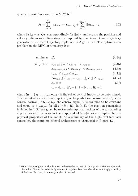
quadratic cost function in the MPC is2

Jk =

Hp∑m=1

||xk+m − rk+m||2Q +

Hc−1∑m=0

||uk+m||2R, (4.2)

where ||x||Q = xTQx, correspondingly for ||u||R, and rm are the position andvelocity references at time step m computed by the time-optimal trajectorygenerator or the local trajectory replanner in Algorithm 1. The optimizationproblem in the MPC at time step k is

minimizeUk

Jk (4.3a)

subject to xk+m+1 = Axk+m +Buk+m (4.3b)

xk+m+1,min ≤ xk+m+1 ≤ xk+m+1,max (4.3c)

umin ≤ uk+i ≤ umax, (4.3d)

∆umin ≤ (uk+i − uk+i−1)/T ≤ ∆umax (4.3e)

xk = x (4.3f)

m = 0, . . . ,Hp − 1, i = 0, . . . ,Hc − 1

where Uk = uk, . . . , uk+Hc−1 is the set of control inputs to be determined,x is the initial state at time step k, Hp is the prediction horizon, and Hc is thecontrol horizon. If Hc < Hp, the control signal ui is assumed to be constantand equal to uk+Hc−1 for all i ≥ k + Hc. In (4.3), the position constraintsincluded in (4.3c) are given by rectangular approximations of the surroundinga priori known obstacles in the map, and (4.3d)–(4.3e) are implied by thephysical properties of the robot. As a summary of the high-level feedbackcontroller, the complete control architecture is visualized in Figure 4.2.

2 We exclude weights on the final state due to the nature of the a priori unknown dynamicobstacles. Given the vehicle dynamics, it is plausible that this does not imply stabilityviolations. Further, it is easily added if desired.

27

Chapter 4. High-Level Feedback Controller

TGPath

MPCr

Cu

Vehicleτ

φ, δxp

Figure 4.2 The control architecture. A path planner provides the tra-jectory generator (TG) with a desired path. The trajectory generator com-putes corresponding time-optimal trajectories, which are sent to the MPC.The internal wheel controllers, C, transform the Cartesian velocities to therespective wheel. Based on these references, wheel torques are computed.The trajectory generator only computes new trajectories when a new pathis available.

28

5Experimental Results

To validate the proposed approach to trajectory generation, path tracking,and obstacle avoidance for four-wheeled vehicles, the methods discussed inSecs. 3–4 were implemented and subsequently experimentally verified in arelevant scenario on a pseudo-omnidirectional mobile robot platform. Theparticular scenario was chosen to illustrate the capabilities of the algorithmsin factory-type setups.

5.1 Experimental Setup

The robot employed for the experimental validation was a four-wheeledpseudo-omnidirectional mobile robot equipped with eight motors, two foreach wheel realizing the steering and driving, see Figure 5.1. The mobile robot[Weisshardt and Garcia, 2014], which was built and designed at FraunhoferIPA in Stuttgart, is the successor to the Care-O-Bot 3 mobile base [Con-nette et al., 2009; Weisshardt and Garcia, 2014]. It was equipped with twoSICK S300 laser scanners, which delivered laser-range measurements fromthe front and rear corners of the robot. The robot was controlled and sensordata were acquired using the ROS software package [WillowGarage, 2015].The wheel-encoder position and velocity measurements were extracted at arate of 100 Hz. The individual wheels were controlled with torque-resolvedcascaded position and velocity controllers running at 100 Hz. The controllerswere implemented in C++ and executed internally in ROS. To estimate theparameters in the effective inertia matrix Ie(ξ) and Coulomb-friction param-

eter vector F ξC required for the robot model in (2.21), experimental data werecollected. Under the assumption that the translational motion of the robotis significantly larger than the rotational motion, the matrix is approximatedto be diagonal with inertia elements

Ie(ξ) = diagIeφ,1, I

eφ,2, I

eφ,3, I

eφ,4, I

eδ,1, I

eδ,2, I

eδ,3, I

eδ,4

, (5.1)

29

Chapter 5. Experimental Results

Figure 5.1 The mobile platform used for the experimental validation,together with one of the items (garbage bin in the background) that servedas obstacles during the experiments. The yellow laser scanners attached totwo of the corners of the robot were used for obstacle detection, localization,and map building.

where diag· is a diagonal matrix with the specified elements along thediagonal. The parameters were estimated by linearly increasing the velocityreferences to the wheel controllers, starting at rest. A linearly increasingvelocity corresponds to a constant applied torque in the robot model. Hencethe inertia elements in the mass matrix can be estimated as the ratio betweenthe applied torque and the corresponding angular acceleration. The motortorque measurements were accessible within the mobile robot platform viaROS. For details regarding estimating F ξC , see [Berntorp et al., 2014a].

5.2 Implementation and Software Architecture

Figure 5.2 shows a schematic representation of the implementation structure.The path planner implemented in ROS generated a feasible geometric path,given a predefined static map of the environment, using Dijkstra’s algorithm[LaValle, 2006]. The map was determined prior to the experiment basedon data from the two laser scanners, attached to the corners of the mobilerobot-platform, combined with the wheel odometry, using the SimultaneousLocalization and Mapping (SLAM) algorithm described in [Grisetti et al.,2007; Grisetti et al., 2005]. The generated path was sent to the time-optimaltrajectory generator, which provided wheel position and velocity trajectories

30

5.3 Path-Tracking Scenario

corresponding to the time-optimal input torques. The wheel-velocity refer-ences given by the trajectory generator were subsequently transformed toCartesian velocity references using the forward differential kinematics. Thesevelocity trajectories and the corresponding position trajectories were thensent to the MPC together with the current estimates of the state vector(pose and velocity), estimated by a particle filter based on the static mapwith the laser-scanner data and the wheel odometry.

The log-barrier solver in Section 3.2 was implemented in Matlab andthen transformed to C code using the Coder toolbox in Matlab and com-piled. The MPC was implemented in C using CVXGEN [Mattingley andBoyd, 2012], which resulted in an average solution time of 1 ms for the modelat hand and the prediction horizons considered (Hp = Hc = 10, correspond-ing to a horizon of 0.4 s, was found to result in desired tracking behavior).Considering the fast solution times for the MPC, longer prediction horizonswould therefore be possible if necessary. Further, it is not the MPC compu-tations that are limiting the choice of sample time, but rather the navigationand computation algorithms in ROS running on the same computer. To linkthe developed controllers with the robot operating system, we employed aPython abstraction of ROS, denoted ROSPy, which executed at a rate of25 Hz. To invoke the trajectory generator and the MPC, both implementedin C, from Python the ctypes library [Python Software Foundation, 2015]was employed.

5.3 Path-Tracking Scenario

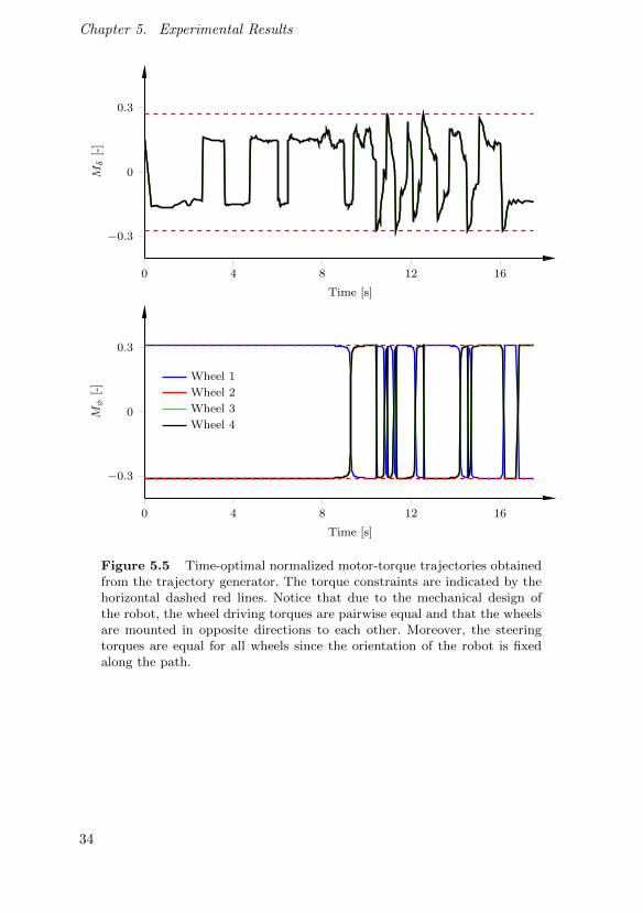
The experiments were performed in a room with an area of approximately75 m2. The map of the room, resulting from application of the SLAM al-gorithm, is shown in Figure 5.3. Based on this map, a geometric path wasplanned from the coordinate (0, 1.5) m to (7,−1.5) m; the orientation of therobot platform was computed such that the robot heading ψ was constantalong the path. The time-optimal trajectory generation was performed, re-sulting in the velocity trajectories shown in Figure 5.4 (expressed in CartesianXY -coordinates). The constraints on the steering actuators were introducedas Mδ,max = 0.27 and on the driving actuators as Mφ,max = 0.31 and sym-metrically for the lower bound. These constraints were chosen based on thephysical properties of the wheel motors in the mobile robot. Note that thewheel torques have been normalized. These constraints were chosen with aslight conservatism to provide actuation capability in the MPC for the obsta-cle avoidance. The corresponding time-optimal torques for the steering anddriving motors are shown in Figure 5.5. Note that at least one input torque isat the limit at each time point, indicating the desired time-optimality [Chenand Desrochers, 1989]. In addition, it is clear that the driving motors are

31

Chapter 5. Experimental Results

ROS

Odometry

Path Planner

Torque-Resolved Velocity Controllers

ROSPy

Obstacle Avoidance

p,v uk

25 HzMPC

uk

xk, rm, m = k, . . . , k +Hp

Trajectory Generator

path

r

Wheel Encoders Laser Scanners

φ, δ Range

100 Hz

Figure 5.2 A sketch of the implementation structure. The odometry,navigation, and torque-resolved velocity controllers can be interacted withthrough ROS. They consist of compiled C++ code. We use a Python ab-straction of ROS, called ROSPy, and connect the MPC and log-barriersolver to ROSPy using compiled C code via the ctypes library.

the limiting factors, which is expected from the geometry of the path withonly limited orientation changes of the wheels. Still, there is significant mo-tion perpendicular to the orientation of the platform, resulting in the steertorques observed in the upper plot in Figure 5.5.

Initially, in the absence of dynamic obstacles, the mobile robot trackedthe nominal path and the time-optimal trajectories using the MPC. Thecontroller parameters (that is, the weight matrices in (4.2)) were chosen as

Q = diag1, 1, 0.1, 0.1, 0.1, 0.1, R = diag0.1, 0.1, 1.

The constraints on the control signal were

umax =(1 1 0.1

)T,

and umin = −umax with the units m/s and rad/s, whereas the slew-rate limitwas chosen as

∆umax =(0.5 0.5 0.05

)T,

32

5.3 Path-Tracking Scenario

−4 −2 0 2 4 6 8

−3

−2

−1

0

1

2

3

X [m]

Y[m

]

Planned Executed

Figure 5.3 The scenario considered for evaluation of the proposed ap-proach to trajectory generation for four-wheeled vehicles. The nominalplanned path is shown together with the actual traversed path, the lat-ter resulting because of the a priori unknown obstacles (red). The mobilerobot hull is displayed (dashed blue) every other second.

0 4 8 12 16

−0.4

0

0.4

0.8

Time [s]

Cart

esia

nV

eloci

ty[m

/s]

pXpY

Figure 5.4 Time-optimal velocity-trajectory references in the CartesianXY -space obtained from the trajectory generator, measured in global co-ordinates.

33

Chapter 5. Experimental Results

0 4 8 12 16

−0.3

0

0.3

Time [s]

Mδ

[-]

0 4 8 12 16

−0.3

0

0.3

Time [s]

Mφ

[-]

Wheel 1

Wheel 2

Wheel 3

Wheel 4

Figure 5.5 Time-optimal normalized motor-torque trajectories obtainedfrom the trajectory generator. The torque constraints are indicated by thehorizontal dashed red lines. Notice that due to the mechanical design ofthe robot, the wheel driving torques are pairwise equal and that the wheelsare mounted in opposite directions to each other. Moreover, the steeringtorques are equal for all wheels since the orientation of the robot is fixedalong the path.

34

5.3 Path-Tracking Scenario

and ∆umin = −∆umax with the units m/s2 and rad/s2. After the robotstarted to move along the nominal path, two new obstacles were placed suchthat they intersected the nominal geometric path (where the obstacle loca-tions are not encoded in the static map defined previously). These obstacleswere instead detected during runtime using the laser scanner sensors. Tominimize the path deviation because of the obstacles, the threshold value ε1was chosen as short as possible; in this case to 400 mm. Further, the pa-rameters c and ε2 in Algorithm 1 were zero in the considered experiment,because the obstacles were assumed to have slowly varying or static posi-tions, rendering the additional term negligible. The executed path is shownin Figure 5.3 together with the map of the environment. The correspondingCartesian velocity references computed by the MPC are shown in Figure 5.6,where also the time instants at which the obstacle avoidance scheme was ac-tivated are displayed. From Figure 5.4 it is clear that the robot is detectingand subsequently avoiding the new obstacles, and also that when followingthe nominal path the time-optimal velocity trajectories are tracked closely.Further, the downmost plot in Figure 5.6 indicates that the coupling betweentranslational and rotational movement is small, implying that the decoupledmodel (4.1) is indeed a valid approximation in this experiment.

35

Chapter 5. Experimental Results

0 5 10 15 20 23

−1

−0.5

0

0.5

Time [s]

pY,ref

[m/s]

0 5 10 15 20 23

−0.5

0

0.5

1

Time [s]

pX,ref

[m/s]

0 5 10 15 20 23

−3

−1.5

0

Time [s]

ψre

f[m

rad

/s]

Figure 5.6 Cartesian velocity commands, measured in the global XY -coordinate system, computed by the MPC based on the time-optimal tra-jectories and the obstacle avoidance scheme. The instants at which switchesbetween path tracking and obstacle avoidance occur are indicated by thevertical dashed red lines. Note that the time-optimal trajectories in Fig-ure 5.4 are closely tracked when not avoiding the new obstacles.

36

6Discussion

A key feature of the considered system architecture is that it combines gener-ation of time-optimal reference trajectories (based on a nonlinear model of thevehicle incorporating friction) with a feedback controller for path tracking,where the problems of finding the reference trajectories and control signalsare posed as convex optimization problems. This implies that an optimal so-lution will be found quickly, enabling high sampling frequencies in the controlarchitecture. Typically, the solution time for the trajectory generator is wellbelow 1 s for paths of approximately 10 m (resulting in L = 500 discretiza-tion elements in the optimization problem (3.9)), and the solution time forthe MPC is almost always within 1 ms (corresponding to 5–10 iterations)for the scenarios we have tested. In our control architecture, the trajectorygenerator is only executing when a completely new path is required. Thus, amajor part of the time in the motion-planning phase is spent on path plan-ning, since this typically requires significantly longer time than the proposedtrajectory-generation algorithm. Further, considering different optimizationcriteria than time, the trajectory generator can be modified to minimizecombinations of path-traversal time and, for example, energy consumption.In [Grundelius, 2001], it is shown that solution of the minimum-energy opti-mal control problem over a fixed time-horizon, where the final time is chosenslightly longer than the corresponding time-optimal, is beneficial for robust-ness of the control.

Another desired property inherent in the architecture is that the MPCsuppresses the effect of model errors. We showed in [Berntorp et al., 2014a]that the model errors caused by the no-slip assumption are small, but com-bining the proposed approach to time-optimal trajectory generation usinga model without slip decreases the influence of this model limitation evenfurther. Moreover, there are other imperfections present as well, such as un-certainties in the geometry. Since the MPC uses the global pose estimatefor feedback, it effectively decreases the effects of model uncertainties whencombined with the low-level wheel controllers. This is a difference to manyexisting reference implementations in mobile robots, where a reference tra-

37

Chapter 6. Discussion

jectory is generated and then typically fed to the low-level loops withoutglobal feedback from workspace estimates.

As mentioned before, a motivation for using online trajectory and localpath regeneration rather than replanning the complete path when an obstacleis encountered, is that it is sometimes desirable to stay close to the original(nominal) path. Another motivation is that successive replanning and tra-jectory generation might prevent task effectiveness. To demonstrate this, weused the robot’s internal proprietary navigation module and applied it tothe same scenario as considered in Chapter 5. The navigation module hasbeen developed by the robot manufacturer. It is written in C++, and takesfull advantage of the omnidirectional characteristics of the considered robot,but only considers constraints on a kinematic level. Thus, it is not using thefull potential of the wheel motors. Figure 6.1 shows the path traversed bythe robot and Figure 6.2 shows the Euclidean norm of the velocity vectoralong the path. The same scenario that takes approximately 25 s to com-plete with our architecture now demands roughly 60 s. The longer executiontime for the reference method is expected since the objective is not time-optimality. Moreover, there are more restrictive velocity constraints in theinternal navigation module than in the approach presented in this report.More interesting, however, is that the robot stops and finds new feasiblepaths three times in total, with each replanning lasting about 1 s. Hence, itis clear that an approach that performs online collision avoidance based onlocal regeneration of the trajectory is advantageous when task effectiveness isdesired. By inspection of Figure 6.1 it is also obvious that the resulting geo-metric path differs significantly from the nominal path, shown in Figure 5.3.In addition, note that if it really is desired to initialize a replanning of thepath and trajectories when an obstacle is encountered, this is easily achiev-able with the trajectory generator in this report, which enables fast solutiontimes for the reoptimization of the trajectory. Hence, it can be used togetherwith the low-level wheel controllers to improve the current implementationof the navigation module.

The considered approach was verified and evaluated on a mobile-robotsetup, employing relatively low velocities, which are typical for mobile robotsin industrial production and manufacturing shop floors. However, the archi-tecture could be valid for more scenarios where four-wheeled vehicles withindependent steering and driving are employed. When considering vehicleplatooning the routes are predetermined using maps of the available paths,the global positions are received from a global positioning system, and obsta-cles are typically detected using vision and/or sonar measurements. In thesecases, it is not time-optimality alone that is the objective. Rather, it shouldbe combined with other criteria, such as energy consumption, and with con-straints on the acceleration and the jerk of the vehicle to allow for smoothand stable driving.

38

Chapter 6. Discussion

0 2 4 6

−2

−1

0

1

2

X [m]

Y[m

]

Figure 6.1 Resulting geometric path for the CoG when instead usingthe internal navigation module in the considered mobile robot platform ina comparative study. The locations at which replanning of the path occursare marked with blue +. The motion is performed from the coordinate(0, 1.5) m to (7,−1.5) m.

0 8 15 20 40 60

0

0.1

0.2

Time [s]

‖v‖ 2

[m/s]

Figure 6.2 Euclidean norm of the velocity vector when instead using theconsidered robot’s internal navigation module in a comparative study forthe scenario in Figure 5.3. In contrast to the architecture in this report, therobot stops for replanning purposes at t = 8, 15, and 20 seconds.

39

7Conclusions

We have considered an approach to time-optimal trajectory generation andonline path tracking with obstacle avoidance for four-wheeled vehicles withindependent steering and driving. The approach is based on convex opti-mization, allowing fast computations both for trajectory generation and on-line control. The obstacle-avoidance scheme was integrated in a high-levelfeedback controller based on MPC. The proposed architecture was fully im-plemented on a pseudo-omnidirectional mobile platform and evaluated in ex-periments in a demanding path-tracking scenario. The method was shown toperform well, and exhibited several advantages in comparison to a referencemethod, especially in terms of traversal time and velocity smoothness.

41

Acknowledgments

Bjorn Olofsson and Anders Robertsson are members of the LCCC LinnaeusCenter and the ELLIIT Excellence Center at Lund University. This researchwas supported by the Swedish Foundation for Strategic Research throughthe project ENGROSS and the European Commission’s Seventh FrameworkProgram under grant agreement SMErobotics (ref. #287787). This researchwas not sponsored by Mitsubishi Electric or any of its subsidiaries.

43

Bibliography

Ardeshiri, T, M Norrlof, J Lofberg, and A Hansson (2011). “Convex opti-mization approach for time-optimal path tracking of robots with speeddependent constraints”. In: Proc. IFAC World Congress. Milano, Italy,pp. 14648–14653.

Berntorp, K, B Olofsson, and A Robertsson (2014a). “Path tracking withobstacle avoidance for pseudo-omnidirectional mobile robots using con-vex optimization”. In: Proc. Am. Control Conf. (ACC). Portland, OR,pp. 517–524.

Berntorp, K. and F. Magnusson (2015). “Hierarchical predictive control forground-vehicle maneuvering”. In: Proc. American Control Conf. Chicago,IL, pp. 2771–2776.

Berntorp, K., B. Olofsson, K. Lundahl, and L. Nielsen (2014b). “Modelsand methodology for optimal trajectory generation in safety-critical road–vehicle manoeuvres”. Vehicle System Dynamics 52:10, pp. 1304–1332.

Bobrow, J. E., S Dubowsky, and J. S. Gibson (1985). “Time-optimal controlof robotic manipulators along specified paths”. Int. J. Robotics Research4:3, pp. 3–17.

Boyd, S. and L. Vandenberghe (2004). Convex Optimization. 6th ed. Cam-bridge Univ. Press, Cambridge, UK.

Castro, R. de, M. Tanelli, R. E. Araujo, and S. M. Savaresi (2014).“Minimum-time path following in highly redundant electric vehicles”. In:Proc. IFAC World Congress. Cape Town, South Africa, pp. 3918–3923.

Chen, Y. and A. A. Desrochers (1989). “Structure of minimum-time controllaw for robotic manipulators with constrained paths”. In: Proc. IEEE Int.Conf. Robotics and Automation (ICRA). Scottsdale, AZ, pp. 971–976.

Choi, J.-W., R. E. Curry, and G. H. Elkaim (2009). “Obstacle avoiding real-time trajectory generation and control of omnidirectional vehicles”. In:Proc. Am. Control Conf. (ACC). St. Louis, MI, pp. 5510–5515.

45

Bibliography

Connette, C. P., C. Parlitz, M. Hagele, and A. Verl (2009). “Singular-ity avoidance for over-actuated, pseudo-omnidirectional, wheeled mobilerobots”. In: Proc. IEEE Int. Conf. Robotics and Automation (ICRA).Kobe, Japan, pp. 1706–1712.

Connette, C. P., S. Hofmeister, A. Bubeck, M. Hagele, and A. Verl (2010).“Model-predictive undercarriage control for a pseudo-omnidirectional,wheeled mobile robot”. In: Proc. 41st Int. Symp. Robotics (ISR) and 6thGerman Conf. Robotics (ROBOTIK). Munich, Germany, pp. 1–6.

CVX Research Inc. (2015). CVX: matlab software for disciplined convex pro-gramming, version 2.0 beta. http://cvxr.com/cvx, Accessed: 2015-01-12.

Dahl, O. (1992). Path Constrained Robot Control. ISRN LUTFD2/TFRT--1038--SE. PhD thesis. Department of Automatic Control, Lund Univer-sity, Sweden.

Dahl, O. (1993). “Path constrained motion optimization for rigid and flex-ible joint robots”. In: Proc. IEEE Int. Conf. Robotics and Automation(ICRA). Atlanta, GA, pp. 223–229.

Dahl, O. and L. Nielsen (1990). “Torque limited path following by on-linetrajectory time scaling”. IEEE Trans. Robot. and Autom. 6:5, pp. 554–561.

Debrouwere, F., W. Van Loock, G. Pipeleers, Q. Tran Dinh, M. Diehl, J. DeSchutter, and J. Swevers (2013). “Time-optimal path following for robotswith convex-concave constraints using sequential convex programming”.IEEE Trans. Robot. 29:6, pp. 1485–1495.

Fox, D., W. Burgard, and S. Thrun (1997). “The dynamic window approachto collision avoidance”. IEEE Robot. Autom. Mag. 4:1, pp. 23–33.

Golub, G. H. and C. F. Van Loan (1996). Matrix Computations. 3rd ed. TheJohns Hopkins Univ. Press, Baltimore, MD.

Grant, M. and S. Boyd (2008). “Graph implementations for nonsmooth con-vex programs”. In: Blondel, V. et al. (Eds.). Recent Advances in Learningand Control. Springer-Verlag, Berlin, Heidelberg, Germany, pp. 95–110.

Grisetti, G., C. Stachniss, and W. Burgard (2005). “Improving grid-basedSLAM with Rao-Blackwellized particle filters by adaptive proposals andselective resampling”. In: Proc. IEEE Int. Conf. Robotics and Automation(ICRA). Barcelona, Spain, pp. 2432–2437.

Grisetti, G., C. Stachniss, and W. Burgard (2007). “Improved techniquesfor grid mapping with Rao-Blackwellized particle filters”. IEEE Trans.Robot. 23, pp. 34–46.

Grundelius, M. (2001). Methods for Control of Liquid Slosh. ISRNLUTFD2/TFRT--1062--SE. PhD thesis. Department of AutomaticControl, Lund University, Sweden.

46

Bibliography

Howard, T., C. Green, and A. Kelly (2009). “Receding horizon model-predictive control for mobile robot navigation of intricate paths”. In: Proc.7th Int. Conf. Field and Service Robotics. Cambridge, MA.

Kanjanawanishkul, K. and A. Zell (2009). “Path following for an omnidirec-tional mobile robot based on model predictive control”. In: Proc. IEEEInt. Conf. Robotics and Automation (ICRA). Kobe, Japan, pp. 3341–3346.

Kant, K. and S. W. Zucker (1986). “Toward efficient trajectory planning: thepath-velocity decomposition”. Int. J. Robotics Research 5:3, pp. 72–89.

Khatib, O. (1986). “Real-time obstacle avoidance for manipulators and mo-bile robots”. Int. J. Robotics Research 5:1, pp. 90–98.

Klancar, G. and I. Skrjanc (2007). “Tracking-error model-based predictivecontrol for mobile robots in real time”. Robotics and Autonomous Systems55:6, pp. 460–469.

LaValle, S. M. (2006). Planning Algorithms. Cambridge Univ. Press, Cam-bridge, UK.

Lipp, T. and S. Boyd (2014). “Minimum-time speed optimization over a fixedpath”. Int. J. Control 87:6, pp. 1297–1311.

Maciejowski, J. M. (1999). Predictive Control with Constraints. Addison-Wesley, Boston, MA.

Mattingley, J. and S. Boyd (2012). “CVXGEN: A Code Generator for Embed-ded Convex Optimization”. Optimization and Engineering 13:1, pp. 1–27.

Mayne, D. Q., J. B. Rawlings, C. V. Rao, and P. O. Scokaert (2000). “Con-strained model predictive control: stability and optimality”. Automatica36:6, pp. 789–814.

Noren, C. (2013). Path Planning for Autonomous Heavy Duty Vehiclesusing Nonlinear Model Predictive Control. LiTH-ISY-EX–13/4707–SE.Linkoping Univ., Linkoping, Sweden.

Oftadeh, R, R Ghabcheloo, and J Mattila (2014). “Time optimal path fol-lowing with bounded velocities and accelerations for mobile robots withindependently steerable wheels”. In: Proc. IEEE Int. Conf. Robotics andAutomation (ICRA). Hong Kong, China, pp. 2925–2931.

Pacejka, H. B. (2006). Tire and Vehicle Dynamics. 2nd ed. Butterworth-Heinemann, Oxford, United Kingdom.

Pfeiffer, F. and R. Johanni (1987). “A concept for manipulator trajectoryplanning”. IEEE J. Robot. Autom. 3:2, pp. 115–123.

Python Software Foundation (2015). Ctypes — A foreign function library forPython. http://docs.python.org/2/library/ctypes.html, Accessed: 2015-01-12.

47

Bibliography

Qu, Z., J. Wang, and C. E. Plaisted (2004). “A new analytical solution tomobile robot trajectory generation in the presence of moving obstacles”.IEEE Trans. Rob. 20:6, pp. 978–993.

Quinlan, S. and O. Khatib (1993). “Elastic bands: connecting path plan-ning and control”. In: Proc. IEEE Int. Conf. Robotics and Automation(ICRA). Atlanta, GA, pp. 802–807.

Schindler, E. (2007). Fahrdynamik: Grundlagen Des Lenkverhaltens Und IhreAnwendung Fur Fahrzeugregelsysteme. Expert-Verlag, Renningen, Ger-many.

Shin, K. G. and N. D. McKay (1985). “Minimum-time control of robotic ma-nipulators with geometric path constraints”. IEEE Trans. Autom. Control30:6, pp. 531–541.

Spong, M. W., S. Hutchinson, and M. Vidyasagar (2006). Robot Modelingand Control. John Wiley and Sons, Hoboken, NJ.

The Orocos Project (2015). Orocos—Open robot control software. Accessed:2015-01-12. url: http://www.orocos.org.

Van Loock, W., G. Pipeleers, and J. Swevers (2013). “Time-optimal pathplanning for flat systems with application to a wheeled mobile robot”. In:Proc. Workshop Robot Motion and Control (RoMoCo). Wasowo, Poland,pp. 192–196.

Verscheure, D., B. Demeulenaere, J. Swevers, J. De Schutter, and M. Diehl(2008). “Time-energy optimal path tracking for robots: a numericallyefficient optimization approach”. In: Proc. 10th Int. Workshop AdvancedMotion Control. Trento, Italy, pp. 727–732.

Verscheure, D., M. Diehl, J. De Schutter, and J. Swevers (2009a). “On-line time-optimal path tracking for robots”. In: Proc. IEEE Int. Conf.Robotics and Automation (ICRA). Kobe, Japan, pp. 599–605.

Verscheure, D., M. Diehl, J. De Schutter, and J. Swevers (2009b). “Recur-sive log-barrier method for on-line time-optimal robot path tracking”. In:Proc. Am. Control Conf. (ACC). St. Louis, MI, pp. 4134–4140.

Verscheure, D., B. Demeulenaere, J. Swevers, J. De Schutter, and M. Diehl(2009c). “Time-optimal path tracking for robots: a convex optimizationapproach”. IEEE Trans. Autom. Control 54:10, pp. 2318–2327.

Wang, Y. and S. Boyd (2010). “Fast model predictive control using onlineoptimization”. IEEE Trans. Control Syst. Technol. 18:2, pp. 267–278.

Weisshardt, F. and N. H. Garcia (2014). Care-O-bot Manual: Manual forCare-O-bot users and administrators. Fraunhofer IPA, Institute for Man-ufacturing Engineering and Automation, Stuttgart, Germany.

WillowGarage (2015). Robot Operating System. Accessed: 2015-01-12. url:http://www.ros.org.

48

Bibliography

Yuille, A. L. and A. Rangarajan (2003). The Concave-Convex Procedure.Vol. 15. 4. Neural Computation, MIT Press, Cambridge, MA, pp. 915–936.

49