HAL Id: hal-02493513https://hal.archives-ouvertes.fr/hal-02493513

Preprint submitted on 27 Feb 2020

HAL is a multi-disciplinary open accessarchive for the deposit and dissemination of sci-entific research documents, whether they are pub-lished or not. The documents may come fromteaching and research institutions in France orabroad, or from public or private research centers.

L’archive ouverte pluridisciplinaire HAL, estdestinée au dépôt et à la diffusion de documentsscientifiques de niveau recherche, publiés ou non,émanant des établissements d’enseignement et derecherche français ou étrangers, des laboratoirespublics ou privés.

A continuum active structure model for the interactionof cilia with a viscous fluid

Astrid Decoene, Sébastien Martin, Fabien Vergnet

To cite this version:Astrid Decoene, Sébastien Martin, Fabien Vergnet. A continuum active structure model for theinteraction of cilia with a viscous fluid. 2020. hal-02493513

A continuum active structure model for the interaction of cilia

with a viscous fluid

Astrid Decoene∗, Sebastien Martin†, Fabien Vergnet‡

February 27, 2020

Abstract

This paper presents a modeling, analysis and simulation of a fluid-structure interaction model with an activethin structure, reproducing the behaviour of cilia or flagella immersed in a viscous flow. In the context oflinear or nonlinear elasticity, the model is based upon the definition of a suitable internal Piola-Kirchoff tensormimicking the action of the internal dyneins that induce the motility of the structure. In the subsequent fluid-structure interaction problem, two difficulties arise: on the one hand the internal activity of the structure whichleads to more restricted well-posedness conditions and, on the other hand, the coupling conditions between thefluid and the structure that require a specific numerical treatment. In the context of numerical simulation, aweak formulation of the time-discretized problem is derived in functional frameworks that include the couplingconditions but, for numerical purposes, an equivalent formulation using Lagrange multipliers is introduced inorder to get rid of the constraints in the functional spaces: this new formulation allows for the use of standard(fluid and structure) solvers, up to an iterative procedure. Numerical simulations are presented, including thebeating of one or two cilia in 2d, discussing the competition between the magnitude of the internal activity andthe viscosity of the surrounding fluid.

Keywords. Stokes flow, elasticity, fluid-structure interaction, active structure, numerical simulationMSC. 74F10, 76Z05, 76D07, 74B20, 65M60, 74H15

1 Introduction

Cilia and flagella are motile elongated structures, involved in swimming and/or transport mechanisms that arisein many living organisms. Flagella are usually used by micro-swimmers such as sperm-cells, bacteria or algae formotility purpose at low Reynolds number, while cilia are generally involved in the transport of proteins, nutrientsor dust inside bigger organisms. At the origin of all these mechanisms are two essential ingredients. The first oneis the capacity for cilia and flagella to modify their shapes by generating active internal deformations and stresses,even without external load. The second one is the strong reciprocal interaction between these structures and thesurrounding fluid. The problem we are interested in is the capacity of such microorganisms to deform themselvesby mean of internal biological motors and to interact with the surrounding fluid. In the present article, we present amodel for the actuation of elongated cilia-like structures, which fits within the framework of continuum mechanics,and study the fluid-structure interaction problem they are involved in.

Eukaryotic cilia (or flagella) are elongated deformable structures with a typical diameter between 0.1 and 0.3µm, whereas the length of cilia can vary from 5 µm (in the lung [1]), to 80 µm long (for the tail of spermatozoon inmice). Cilia are membrane-bounded structures composed of a microtubule cytoskeleton, called axoneme, consistingof a ring of nine doublets microtubules surrounding a central pair of microtubules. Outer doublets microtubules arelinked to the central pair by radial proteins and to each other by nexin links, which strengthen the structure. Beatingmovements of cilia are induced by internal motors producing a bending in the whole structure, when two outerdoublets microtubules slide with respect to one another. This sliding is produced by proteins, called dyneins, thatare synthesized on one doublet microtubules and attach to the neighboring one. The radial connections resist the

∗Universite Paris-Sud, LMO (CNRS UMR 8628), Batiment 307, 91405 Orsay cedex, France.astrid.decoene@math.u-psud.fr†Universite de Paris, MAP5 (CNRS UMR 8145) & FP2M (CNRS FR 2036), 45 rue des Saints-Peres, 75270 Paris cedex, France.

sebastien.martin@parisdescartes.fr‡Ecole polytechnique, CMAP (CNRS UMR 7641), Route de Saclay, 91128 Palaiseau cedex, France.

fabien.vergnet@polytechnique.edu

1

sliding and contribute to the bending of the structure, since the cilium is anchored at the bottom. This mechanismappears all along the length of a cilium and between all doublets microtubules, which contributes to the emergenceof different sliding patterns and different shapes of deformation for the cilium. The precise nature of the spatialand temporal control mechanisms regulating the various ciliary beats is still unknown [2]. Further details on theinternal structure and mechanisms of cilia can be found in [3].

The presence of ciliary propulsion in almost all living organisms, from bacteria to mammals, has encouragednumerous scientists to model and study this universal phenomenon. The first work in that sense goes back to 1951and is due to Taylor [4], who initiated the mathematical study of microorganism propulsion. This work presentsthe swimming of a extensible sheet in a viscous fluid modeled by the Stokes equations. The author works in therest frame of the sheet, whose deformations are modeled by the propagation of a wave of small amplitude. Thus,the unknown of the problem is the velocity of the fluid far from the sheet, which also represents the velocity of thesheet in the laboratory frame. Extensions to an infinite cylinder [5, 6] and to finite objects [7, 8] have subsequentlybeen studied. When the amplitude of deformations is large, the resistive force theory (also known as local dragtheory) developed in the pioneering work of Gray and Hancock [9], describes the cilia as several cylinders and usesthe linear property of the Stokes equations to compute the flow induced in the fluid. A similar but more accuratemethod is the slender body theory, started by Hancock in [10] and then improved by Lightill in [11], which makesuse of the long and thin geometry of cilia. It consists in modeling a cilium by a distribution of stokeslets and dipoles,which impose a force on the surrounding fluid. This method is also known as the sublayer method or the stokesletmethod and has been extensively applied to the simulation of thin flagellar propulsion when the deformations of thestructure are imposed (see for example [12, 13, 14]). More recently, the immersed boundary method have been usedfor the simulation of thin beating cilia in a Newtonian fluid in [15]. As in the stokeslet method, the idea is to imposea distribution of forces in the fluid. However, in that case the force does not come from the slender body theorybut is used to impose the equality of the fluid and solid velocities on the fluid-structure interface. In this work, thevelocity of the structure is imposed and its action on the fluid is studied. A different approach is also considered in[16], where cilia are three-dimensional structures whose deformations are reproduced by solving a one-dimensionaltransport equation. The fluid velocity on the fluid-structure interface is imposed using a penalization method, thusno retro-action from the fluid to cilia is taking into account. In [17] cilia are modeled by thin structures whosedeformations are given by the same transport equation than in [16]. The equality of the fluid and solid velocitieson the fluid-structure interface is imposed with the immersed boundary method and the action of the fluid on thestructure is taken into account by changing the velocity of the structure, but cilia always follow the same beatpattern. In all the works that have been previously mentioned, the cyclic shape change of a cilium is imposedwhereas its beatform should be an emergent property of a coupled system involving the internal mechanisms of thecilium, the elastic properties of the structure and the surrounding viscous fluid.

The first work that attempted to take into account the internal activity of cilia through local deformationsis due to Machin [18]. The cilium is considered as an elastic filament immersed in a viscous fluid, whose actionon the structure is given by the resistive force theory. Moreover the internal activity of the cilium is modeled byadding an active bending moment distributed all along the structure. With the active bending moment, wave-likedisplacements are observed whereas, with a passive elastic filament driven from its proximal end, the forms of thewave do not match the actual shapes of cilia. Thus Machin brought to light the importance of local contractility inthe deformation of cilia; in [19] a modification of this model is proposed, by considering two active filaments withregular cross-connections whose contractility in activated when the passive bending reach a critical value. In [20]a similar three-dimensional model is proposed with a more realistic geometry of the internal structure of a cilium.Subsequently, several class of models have been proposed such that curvature-controlled models [21, 22, 23] andself-oscillatory models [24, 25]. A comprehensive review of these different models is presented in [26].

Another approach is presented in [27] and further studied in [28, 29, 30], where a discrete description of theaxoneme is proposed in two space dimension. The cilium is composed of elastic filaments connected by a finitenumber of springs that represent nexin and dynein links. Then, the deformation of the structure is produced by theconnection scenario of dynein links which depends on the geometry of the structure. At the fluid-structure interfacethe continuity of the velocity is considered and is treated numerically with the immersed boundary method. Asimilar model is considered in [31] and [32] in three dimension, where a precise description of the “9+2” structureof the cilium is proposed. In both works, the emerging beating patterns are realistic.

Unlike all previous works on cilia and self-propelled microorganisms moving in a viscous fluid, we aim to modelthe behavior of active biological structures in the framework of continuum mechanics, without using a detaileddescription of their internal structure. The reasons for this study are twofold. First, since the chemical, biologicaland even mechanical processes for the internal activity of eukaryotic cilia are not yet completely understood, wedo not intend to model the nexin and dynein links at the nanometric scale. Instead, we rather take into account

2

the activity in a more phenomenological manner by mean of an internal stress. The context of two and threedimensional elasticity is particularly suitable to reproduce realistic deformations of cilia and flagella. Second, theframework of continuum mechanics enables to fully consider the fluid-structure interaction, which is one of the mostimportant ingredient of the system and which is often neglected in other studies. The model that we develop in thispaper is suitable for both the mathematical study and the numerical simulation of the fluid-structure interactionwith active structures and a viscous fluid.

The paper is organized as follows. In Section 2 we present the equations of active elasticity that have beenintroduced in biomechanics for the study of biological tissues, but never used or mathematically studied for activemicroorganisms at low Reynolds number. Examples of activity scenarios are illustrated as well. In Section 3,we couple the elasticity equations to the Stokes equations and study the fluid-structure interaction problem. Forthe numerical simulation of active structures beating in a viscous fluid we introduce a saddle-point formulation ofthe problem, where the condition of equality of the fluid and structure velocities on the fluid-structure interfaceis treated by a Lagrangian multiplier. In particular, this enables the use of standard finite element methods andsolvers. In Section 4, we present the numerical resolution process and some numerical results for one and two ciliawith prescribed internal activity. The influences of the viscosity of the surrounding fluid, the phase shift betweeninternal activities and the distance between cilia are investigated.

2 A continuum active structure model

The purpose of the present section is to develop a macroscopic model for the internal activity of cilia-like structures.We start by giving a brief review of these models.

2.1 The active-stress method

For the study of biological tissues, two popular macroscopic approaches are used to model the muscles activity,namely the active-stress and active-strain methods (see [33] for a review). The former consists in adding anactive component to the passive stress tensor usually derived from the strain energy law, while the later adoptsa multiplicative decomposition of the tensor gradient of deformation in which the activation acts as a pre-strain.Both techniques have been extensively used in myocardium, arteries and even face muscles studies ([34, 35, 36, 37]),but, to our knowledge, not in the context of microswimmers.

When the structural organization of the active components in the tissue is known, but rather complicated tomodel individually (as it is the case for cilia), the active-stress method appears to be a more suitable approach.Indeed, in this case, the internal stress can be approximated by averaging the geometric arrangement of the activeelements at the micro scale, in order to exhibit a macroscopic fiber-like structure. Then, we suppose that the activebehavior of the tissue is only due to elastic deformations in the direction of these fiber-like structures, which arecalled active fibers. More precisely, if ea denotes a unit vector field in the direction of active fibers within the tissue,which depends on the material position and the time, the active stress tensor, which is denoted by Σ∗, writes

Σ∗ = Σaea ⊗ ea,

where Σa is a scalar function, which also depends on the time and the material position, and ⊗ denotes the tensorproduct. Thus, in the general case, the internal activity is given by a scalar function Σa, that we call the activityscenario, and by a unit vector field ea which, at each material point, points in the direction of active fibers. Formore information on models for contractile organs, see [38, Chapter 2] and references therein.

2.2 The problem of active elasticity

Let Ωs be a Lipschitz open connected bounded subset of Rn, with n ∈ 2, 3. Its boundary, ∂Ωs, is divided in twoparts denoted Γ and Γs such that the boundaries satisfy ∂Ωs = Γ∪Γs and Γ∩Γs = ∅. Moreover we denote by ns theexterior unit normal vector to Ωs. We suppose that Ωs is filled with an elastic active medium, subjected to a timedependent body force, denoted by fs. The internal activity of the structure Σ∗ is described using the active-stressmethod and is supposed to depend only on the time and the material position. Then, the quasi-static problem ofactive elasticity with homogeneous Dirichlet and Neumann boundary conditions, is to find the displacement of thestructure ds, solution for all time t ≥ 0, of the following set of equations:

−div((I +∇ds(t))(Σs(ds(t))− Σ∗(t))) = fs(t), in Ωs,(I +∇ds(t))(Σs(ds(t))− Σ∗(t))ns = 0, on Γ,

ds(t) = 0, on Γs.(1)

3

The matrix I is the identity matrix of Rn and Σs(ds(t)) is the so-called second Piola-Kirchhoff stress tensor attime t, which describes the passive elastic behavior of the structure. For simplicity, we will always assume that theelastic medium follows the Saint Venant-Kirchhoff law, i.e. that the second Piola-Kirchhoff stress tensor writes

Σs(ds(t)) = 2µsE(ds(t)) + λstr(E(ds(t)))I,

E(ds(t)) =1

2(∇ds(t) +∇ds(t)T +∇ds(t)T∇ds(t)),

(2)

where µs > 0 and λs > 0 are Lame’s parameters and E(ds(t)) is known as the Green-Lagrange strain tensor attime t. The elasticity parameters are usually given by mean of Young’s modulus Es, which represents the stiffnessof the medium, and Poisson’s ratio νs, which represents its compressibility:

µs =Es

2(1 + νs), λs =

Esνs(1 + νs)(1− 2νs)

.

Problem (1) differs from the classical elasticity equations by the presence of the stress tensor Σ∗, which acts intwo different ways on the structure. First, it modifies the resulting forces that act on the structure by adding abody force which writes div(Σ∗(t)) in Ωs and a surface force which writes Σ∗(t)ns on Γ. Second, it modifies theelasticity operator by adding the term div(∇ds(t)Σ∗(t)) in the left-hand side of the continuity equation.

In particular, if the body force fs is null, a displacement d∗ which satisfies

Σs(d∗(t, x)) = Σ∗(t, x), ∀t ≥ 0, ∀x ∈ Ωs,d∗(t, x) = 0, ∀t ≥ 0, ∀x ∈ Γs,

is a solution of problem (1). This means that the internal activity acts as a constraint on the second Piola-Kirchhoffstress. At the infinitesimal scale, the second Piola-Kirchhoff stress describes the forces in the reference configurationthat each particle of the elastic medium applies on its neighbors by unit area in the reference configuration. Thus,the active stress tensor Σ∗ can be seen as a constraint on the internal forces that neighboring particles exert oneach other.

2.3 Application to cilia-like structures

In the present study, a cilium-like structure is supposed to be an elastic active medium whose passive componentsatisfies the Saint Venant-Kirchhoff law and whose reference configuration, Ωs, is a straight vertical cylinder offinite length. Moreover, the structure is supposed to be anchored at its bottom boundary, denoted Γs, and wedenote by Γ the remaining of the boundary. In order to model the internal activity of the cilium-like structure, weapply the active-stress method, based on the knowledge of the biological structure of cilia. As we explained, thebending mechanics inside a cilium comes from the activation of several molecules which ends up in the sliding ofthe microtubules, the elongated rod-like structures located at the periphery of the cilium. At a more macroscopicscale, these dynamics can be seen as local elastic deformations in the direction of the microtubules which induce,because the cilium is anchored at the bottom, a bending deformation.

As a consequence, we suppose that a cilium is embedded with vertical active fibers. Then the unit vector field eais constant, in time and in space, and the active stress tensor Σ∗ is given by

Σ∗(t, x) = Σa(t, x)ea ⊗ ea, t ≥ 0, x ∈ Ωs, (3)

where the activity scenario Σa is a scalar field which only depends on the time and the material position in thereference configuration Ωs. In particular, if the activity scenario is constant in time and in space, this inducesan elongation or a contraction of the whole structure in the direction given by ea, depending on the sign of Σa.If Σa is positive the solid stretches, whereas if Σa is negative it shrinks. More generally, at a given time t and at agiven point x, the sign of Σa(t, x) indicates whether the structure locally expanses or contracts. Thus, in the case ofcilia-like bodies, we propose a model for active structures that only depends on the choice of an activity scenario Σa.In particular, this enables to easily reproduce biomimetic self-induced deformations of elongated elastic structures.

2.4 Examples of internal activity

In this subsection, we aim to mimic the characteristic flapping deformations of cilia and flagella. Since the structureis anchored at the bottom, the local expansion or shrinking of the medium should induce the bending of the wholestructure, if the activity scenario is well-chosen. Let Lc > 0 be the length of the cilium-like structure, rc > 0 be its

4

radius and xc be its mean position on the abscissa axis. Then, in two space dimensions, Ωs is the rectangle definedby

Ωs =

(x1, x2) ∈ R2;xc − rc ≤ x1 ≤ xc + rc, 0 ≤ x2 ≤ Lc

. (4)

Moreover, we suppose that the structure is anchored at x2 = 0. We recall that in the case of a cilium-like structure,all active fibers are oriented in the direction of the vector ea = (0, 1).

Bending The first scenario that we study is the case of the periodic (in time) bending of a two-dimensionalstructure. We consider a scenario which only depends on the time and on the first coordinate x1 and which isproportional to the difference xc − x1. It writes

Σa(t, (x1, x2)) =Ca

Lcrcsin(2πfat)(xc − x1), ∀t ≥ 0, ∀(x1, x2) ∈ Ωs, (5)

where fa is the beating frequency and Ca > 0 is the intensity of the internal activity. Actually, if the sign of sin(2πfat)is positive, the structure locally stretches in the half-domain defined by

(x1, x2);xc − rc ≤ x1 < xc, 0 ≤ x2 ≤ Lc

and locally shrinks in the half-domain defined by

(2xc − x1, x2);xc < x1 ≤ xc + rc, 0 ≤ x2 ≤ Lc .

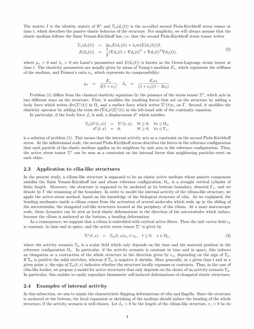
Thus, because the cilium is anchored at the bottom, it ends in the bending of the whole structure to the right. Onthe contrary, if the sign of sin(2πfat) is negative, the cilium bends to the left. To illustrate this bending behavior, wenumerically solve problem (1) with Σa defined by (5) and ea = (0, 1). To that aim we use the finite element methodwith P1 elements and a Newton solver to handle the nonlinear elasticity operator. The resulting deformations ofthe structure are presented in Fig. 1, with the set of parameters be given in Table 1.

Lc (µm) rc (µm) xc (µm) Ca (pN · µm2) fa (Hz) Es νs (pN · µm−2)6.5 0.2 0 1.3 10 106 0.49

Table 1: Set of parameters for the bending scenario of activity.

The elasticity parameters µs and λs are given by Young’s modulus Es and Poisson’s ratio νs. The chosen valueof Poisson’s ratio means that the structure is nearly incompressible. For Young’s modulus, this value comes fromexperimental studies [39]. The activity scenario is plotted on the mesh of the structure. For a time t between 0s and0.025s, we observe in Fig. 1 that the cilium bends to the right, since the sign of sin(2πfat) is positive. For greatervalues of t, the structure returns to its reference configuration while sin(2πfat) decreases and starts to bend to theleft when the sign of sin(2πfat) becomes negative. At t = 0.1s the structure is back in its reference configurationand is about to bend to the right one more time.

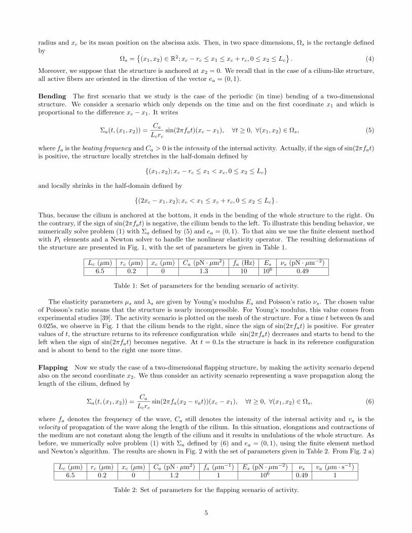
Flapping Now we study the case of a two-dimensional flapping structure, by making the activity scenario dependalso on the second coordinate x2. We thus consider an activity scenario representing a wave propagation along thelength of the cilium, defined by

Σa(t, (x1, x2)) =Ca

Lcrcsin(2πfa(x2 − vat))(xc − x1), ∀t ≥ 0, ∀(x1, x2) ∈ Ωs, (6)

where fa denotes the frequency of the wave, Ca still denotes the intensity of the internal activity and va is thevelocity of propagation of the wave along the length of the cilium. In this situation, elongations and contractions ofthe medium are not constant along the length of the cilium and it results in undulations of the whole structure. Asbefore, we numerically solve problem (1) with Σa defined by (6) and ea = (0, 1), using the finite element methodand Newton’s algorithm. The results are shown in Fig. 2 with the set of parameters given in Table 2. From Fig. 2 a)

Lc (µm) rc (µm) xc (µm) Ca (pN · µm2) fa (µm−1) Es (pN · µm−2) νs va (µm · s−1)6.5 0.2 0 1.2 1 106 0.49 1

Table 2: Set of parameters for the flapping scenario of activity.

5

a)

-0.1

0

0.1

-0.20

0.20

activity

b)

-0.1

0

0.1

-0.20

0.20

activity

c)

-0.1

0

0.1

-0.20

0.20

activity

Figure 1: Bending of an elongated elastic structure with the internal activity given by (5) at different times:a) t = 0s, b) t = 0.012s and c) t = 0.025s. The activity scenario Σa is plotted, with the set of parameters be givenin Table 1.

to d) we observe that, while the wave propagates along the length of the cilium, the structure deforms itself withan oscillatory motion. For example, in Fig. 2 c), the sign of the activity scenario changes along the direction ofthe active fibers and is zero at approximate mid-point of the length of the cilium. This results in a double curveddeformation of the structure since two opposite contraction behaviors are induced by the internal activity: at thebottom of the cilium the medium stretches in the left and contracts in the right, whereas at the top it contracts inthe left and stretches in the right.

A non symmetric scenario In the study of the locomotion of microorganisms, it is well-known that in order toefficiently swim or propel the surrounding fluid, the movement of a cilium or a flagellum has to be non symmetricin time. This is the statement of Purcell’s scallop Theorem [40] and this is due to reversibility properties of viscousfluids at low Reynold’s number (which is the case we are interested in). Thus, to be able to model non symmetricinternal activities is of primary importance for the study of active structures in a viscous fluid. In particular, wepropose an activity scenario to mimic the deformations of cilia:

Σa(t, (x1, x2)) =Ca

Lcrc(σa,1(t, x2) + σa,2(t, x2)) (xc − x1), ∀t ≥ 0, ∀(x1, x2) ∈ Ωs, (7)

where σa,1(t, x2) and σa,2(t, x2) are defined, for all t ≥ 0 and for all x2 in [0, Lc] by

σa,1(t, x2) = (x2 − Lc)2 sin

(2πfa

(t− Ta

4

)),

and

σa(t, x2) =

x2

(x2 −

Lc

2

)cos

(2πfa

(t− Ta

4

)), if t−

⌊t

Ta

⌋Ta ≥

1

2,

0, otherwise.

As before, fa and Ca still denote the beating frequency and the intensity of the internal activity. The parameters Tais the period of the beating, i.e. Ta = 1

fa. The results shown in Fig. 3 correspond to the set of parameters given

in Table 3. They have been obtained by solving problem (1) with Σa defined by (7) and using the finite element

Lc (µm) rc (µm) xc (µm) Ca (pN · µm) fa (Hz) Es (pN · µm−2) νs6.5 0.2 0 3 10 106 0.49

Table 3: Set of parameters for the non symmetric scenario of activity.

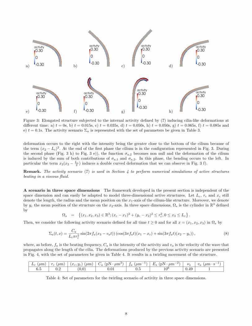
method combined with a Newton’s algorithm. We can observe that the activity scenario (7) is divided in twophases. During the first phase (Fig. 3 a) to Fig. 3 d)), taking place during the first half period of the beat, thefunction σa,2 is null and the cilium starts from a deformed configuration represented in Fig. 3 a). Then a bending

6

a) b)

c) d)

Figure 2: Deformation of an elongated structure subjected to the internal activity defined by (6) at different times:a) t = 0s, b) t = 0.012s, c) t = 0.025s and d) t = 0.037s. The activity scenario Σa is represented with the set ofparameters be given in Table 2.

7

a) b) c) d)

e) f) g) h)

Figure 3: Elongated structure subjected to the internal activity defined by (7) inducing cilia-like deformations atdifferent time: a) t = 0s, b) t = 0.015s, c) t = 0.035s, d) t = 0.050s, h) t = 0.050s, g) t = 0.065s, f) t = 0.085s ande) t = 0.1s. The activity scenario Σa is represented with the set of parameters be given in Table 3.

deformation occurs to the right with the intensity being the greater close to the bottom of the cilium because ofthe term (x2 − Lc)

2. At the end of the first phase the cilium is in the configuration represented in Fig. 3. Duringthe second phase (Fig. 3 h) to Fig. 3 e)), the function σa,2 becomes non null and the deformation of the ciliumis induced by the sum of both contributions of σa,1 and σa,2. In this phase, the bending occurs to the left. Inparticular the term x2(x2 − Lc

2 ) induces a double curved deformation that we can observe in Fig. 3 f).

Remark. The activity scenario (7) is used in Section 4 to perform numerical simulations of active structuresbeating in a viscous fluid.

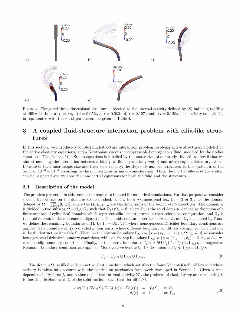
A scenario in three space dimensions The framework developed in the present section is independent of thespace dimension and can easily be adapted to model three-dimensional active structures. Let Lc, rc and xc stilldenote the length, the radius and the mean position on the x1-axis of the cilium-like structure. Moreover, we denoteby yc the mean position of the structure on the x2-axis. In three space dimensions, Ωs is the cylinder in R3 definedby

Ωs =

(x1, x2, x3) ∈ R3; (xc − x1)2 + (yc − x2)2 ≤ r2c , 0 ≤ x3 ≤ Lc

.

Then, we consider the following activity scenario defined for all time t ≥ 0 and for all x = (x1, x2, x3) in Ωs by

Σa(t, x) =Ca

Lcπr2c

sin(2πfa(x3 − vat)) (cos(3πfat)(x1 − xc) + sin(3πfat)(x2 − yc)) , (8)

where, as before, fa is the beating frequency, Ca is the intensity of the activity and va is the velocity of the wave thatpropagates along the length of the cilia. The deformations produced by the previous activity scenario are presentedin Fig. 4, with the set of parameters be given in Table 4. It results in a twirling movement of the structure.

Lc (µm) rc (µm) (xc, yc) (µm) Ca (pN · µm3) fa (µm−1) Es (pN · µm−2) νs va (µm · s−1)6.5 0.2 (0,0) 0.01 0.5 106 0.49 1

Table 4: Set of parameters for the twirling scenario of activity in three space dimensions.

8

a) b) c)

d) e)

Figure 4: Elongated three-dimensional structure subjected to the internal activity defined by (8) inducing twirlingat different time: a) t = 0s, b) t = 0.052s, c) t = 0.082s, d) t = 0.107s and e) t = 0.128s. The activity scenario Σa

in represented with the set of parameters be given in Table 4.

3 A coupled fluid-structure interaction problem with cilia-like struc-tures

In this section, we introduce a coupled fluid-structure interaction problem involving active structures, modeled bythe active elasticity equations, and a Newtonian viscous incompressible homogeneous fluid, modeled by the Stokesequations. The choice of the Stokes equations is justified by the motivation of our study. Indeed, we recall that weaim at modeling the interaction between a biological fluid (essentially water) and microscopic ciliated organisms.Because of their microscopic size and their slow velocity, the Reynolds number associated to this system is of theorder of 10−6 − 10−4 according to the microorganisms under consideration. Thus, the inertial effects of the systemcan be neglected and we consider non-inertial equations for both the fluid and the structures.

3.1 Description of the model

The problem presented in this section is intended to be used for numerical simulations. For that purpose we considerspecific hypotheses on the domains to be meshed. Let Ω be a n-dimensional box (n = 2 or 3), i.e. the domaindefined by Ω =

∏ni=1 [0, Li], where the (Li)i=1,..,n are the dimensions of the box in every directions. The domain Ω

is divided in two subsets, Ω = Ωs∪Ωf such that Ωf ∩Ωs = ∅, where Ωs is the solid domain, defined as the union of afinite number of cylindrical domains which represent cilia-like structures in their reference configuration, and Ωf isthe fluid domain in the reference configuration. The fluid-structure interface between Ωs and Ωf is denoted by Γ andwe define the remaining boundaries of Ωs by Γs = ∂Ωs \ Γ, where homogeneous Dirichlet boundary conditions areapplied. The boundary of Ωf is divided in four parts, where different boundary conditions are applied. The first oneis the fluid-structure interface Γ. Then, on the bottom boundary Γf,D = x = (x1, · · · , xn) ∈ Ω;xn = 0 we considerhomogeneous Dirichlet boundary conditions, while on the top boundary Γf,S = x = (x1, · · · , xn) ∈ Ω;xn = Ln weconsider slip boundary conditions. Finally, on the lateral boundaries Γf,N = ∂Ωf \ (Γ ∪ Γf,D ∪ Γf,S), homogeneousNeumann boundary conditions are applied. Moreover, we denote by Γf the union of Γf,D, Γf,S and Γf,N :

Γf = Γf,D ∪ Γf,S ∪ Γf,N . (9)

The domain Ωs is filled with an active elastic medium which satisfies the Saint Venant-Kirchhoff law and whoseactivity is taken into account with the continuum mechanics framework developed in Section 2. Given a timedependent body force fs and a time dependent internal activity Σ∗, the problem of elasticity we are considering isto find the displacement ds of the solid medium such that, for all t ≥ 0,

−div((I +∇ds(t))(Σs(ds(t))− Σ∗(t))) = fs(t), in Ωs,ds(t) = 0, on Γs,

(10)

9

where Σs(ds(t)) is defined by (2).The solid problem is always solved in the reference configuration of the structure Ωs, i.e. in Lagrangian coordi-

nates, whereas the fluid problem is usually set up in Eulerian coordinates, i.e. in the current (deformed) configura-tion. This deformed configuration at time t ≥ 0 depends on the displacement of the solid medium on the interfaceΓ by means of a transformation denoted by Φ(ds(t)), which satisfies

Φ(ds(t)) = I + ds(t), on Γ.

The mapping I denotes the identity mapping in Rn. Moreover, let γΓ be the trace operator from Ωs onto Γ and Rbe a lifting operator from Γ into Ωf (in spaces made precise later on), then the transformation Φ(ds(t)) is definedin the whole domain Ωf by

Φ(ds(t)) = I +R(γΓ(ds(t))), in Ωf ,

such that R(γΓ(ds(t))) is null on the exterior boundary Γf , defined by (9). Thus, the transformation Φ(ds(t)) mapsthe reference fluid domain Ωf to the deformed fluid domain at time t, Φ(ds(t))(Ωf ). In practice, the constructionof the lifting operator R is done by solving an elliptic problem (typically a Laplace equation or the equations oflinearized elasticity) on Ωf with homogeneous Dirichlet boundary conditions on Γf and applying γΓ(ds(t)) as aDirichlet boundary condition on the interface Γ.

At time t, the domain Φ(ds(t))(Ωf ) is filled with a Newtonian viscous incompressible homogeneous fluid, whoseviscosity, µf , is positive. Given a time dependent body force ff , the velocity of the fluid uf and the pressure of thefluid pf satisfy, for all t ≥ 0, the Stokes equations with mixed Dirichlet, Neumann and slip boundary conditions:

−div(σf (uf (t), pf (t))) = ff (t), in Φ(ds(t))(Ωf ),div(uf (t)) = 0, in Φ(ds(t))(Ωf ),

uf (t) = 0, on Γf,D,uf (t) · nf (t) = 0, on Γf,S ,

(σf (uf (t), pf (t))nf (t)) · τf (t) = 0, on Γf,S ,σf (uf (t), pf (t))nf (t) = 0, on Γf,N .

(11)

The tensor σf (uf (t), pf (t)) is the fluid stress tensor defined by

σf (uf (t), pf (t)) = 2µfD(uf (t))− pf (t)I,

where D(uf (t)) = 12 (∇uf (t) +∇uf (t)T ) is the symmetric gradient of uf (t) and I denotes the identity matrix of Rn.

Equations (10) and (11) are completed by the usual fluid-structure coupling conditions on the interface Γ,namely the equality of the velocities and the continuity of the normal components of stress tensors. Because theseconditions are written in the reference configuration, we introduce the velocity of the fluid written in the fluidreference configuration, wf , and the pressure of the fluid written in the fluid reference configuration, qf , defined by

wf (t, ·) = uf (t,Φ(ds(t, ·))) and qf (t, ·) = pf (t,Φ(ds(t, ·))), in Ωf . (12)

Moreover, the fluid stress tensor at time t written in the fluid reference configuration, denoted by Πf (wf (t), qf (t)),is defined by

Πf (wf (t), qf (t)) = µf

(∇wf (t)F (ds(t)) + (∇(Φ(ds(t))))

−T∇wf (t)TG(ds(t)))− qf (t)G(ds(t)),

where F (ds(t)) and G(ds(t)) are the following matrices:

F (ds(t)) = (∇(Φ(ds(t))))−1cof(∇(Φ(ds(t)))),

G(ds(t)) = cof(∇(Φ(ds(t)))).(13)

Then, for all t ≥ 0, the coupling conditions on Γ write

∂ds(t)

∂t= wf (t), on Γ,

(I +∇ds(t))(Σs(ds(t))− Σ∗(t))ns = Πf (wf (t), qf (t))ns, on Γ.(14)

The condition on the continuity of the velocity through the interface Γ, considered in (14), requires an initialcondition concerning the initial displacement of the structure on Γ. Then, we suppose that all cilia-like structuresare in their reference configuration at time t = 0, i.e. that ds(0) = 0 on Γ.

10

Remark. In problem (11), the current fluid domain Φ(ds(t))(Ωf ) is an unknown of the problem, since it dependson the displacement of the structure. In the present article, we discretize in time equations (10), (11) and (14),in order to make the configuration of the current fluid domain at a given time step entirely determined by thedisplacement of the structure at the previous time step. This is the purpose of the next subsection.

Remark. In definition (13), the matrix F (ds(t)), that appears in the expression of the fluid stress tensor writtenin the fluid reference configuration, is well-defined if the mapping Φ(ds(t)) is, for example, a C1-diffeomorphism.This kind of regularity is not intended to be proved in the present article but it is studied in [41]. In the mean time,we can justify our approach by recalling that our purpose here is to compute numerical simulations based on themodel constructed within the present section and that, in a context of numerical simulations, the deformation at agiven time step is easily invertible. For this reason, we assume in the following that the deformations are regularenough to ensure the definition of the problem.

3.2 The discrete-in-time fluid-structure interaction problem

Let us introduce a discretization of R+ for the time variable t. Let δt > 0 be a constant time step. We construct asequence (tk)k∈N such that

t0 = 0,tk+1 = tk + δt,∀k ≥ 0,

and, for all k ≥ 0, we define the time-discretizations of the displacement of the structure dks , the velocity of thefluid ukf and the pressure of the fluid pkf by

dks ' ds(tk), ukf ' uf (tk), and pkf ' pf (tk).

Similarly, the time-discretization of the body forces fkf and fks and the activity Σ∗k are defined, for all k ≥ 0 by

fkf = ff (tk), fks = fs(tk) and Σ∗k = Σ∗(tk)

Moreover, the first coupling condition in (14) is discretized using the implicit Euler scheme:

d0s = 0,

dk+1s = dks + δtwk+1

f ,∀k ≥ 0.

For k > 0, the deformed fluid domain at time tk, Φ(ds(tk))(Ωf ), is denoted by Ωkf and depends on the displacement

of the structure at the previous time step by

Ωkf = Φ(dk−1

s )(Ωf ).

Similarly, the fluid-structure interface at time tk writes

Γk = Φ(dk−1s )(Γ),

and the remaining fluid boundaries in the deformed configuration do not change, i.e.

Γkf,D = Γf,D,

Γkf,S = Γf,S ,

Γkf,N = Γf,N .

For k = 0, we suppose by convention that d0−1s = 0 on Γ, such that Ω0

f = Ωf and Γ0 = Γ.Then the discrete-in-time fluid-structure interaction problem that we consider is to find, for all k ≥ 0, the

displacement of the structure dks , the velocity of the fluid ukf and the pressure of the fluid pkf which satisfy

−div((I +∇dks)(Σs(dks)− Σ∗k)) = fks , in Ωs,

dks = 0, on Γs,(15)

−div(σf (ukf , pkf )) = fkf , in Ωk

f ,

div(ukf ) = 0, in Ωkf ,

ukf = 0, on Γf,D,

ukf · nkf = 0, on Γf,S ,

(σf (ukf , pkf )nkf ) · τkf = 0, on Γf,S ,

σf (ukf , pkf )nkf = 0, on Γf,N ,

(16)

11

dks = dk−1s + δtwk

f , on Γ,

(I +∇dks)(Σs(dks)− Σ∗k)ns = Πf (wk

f , qkf )ns, on Γ,

(17)

wherewk

f (·) = ukf (Φ(dk−1s )(·)), in Ωf ,

qkf (·) = pkf (Φ(dk−1s )(·)), in Ωf .

In Section 4 we present the numerical method used for the simulation of active structures in a viscous fluid.The method is based on a saddle-point formulation for the discrete-in-time coupled system of equations (15), (16)and (17), that is well-suited for the numerical simulation with standard finite element techniques and solvers, andthat will be introduced later on. To that aim, we first study the weak formulation of problem (15), (16) and (17)in Subsection 3.3, then, the constraint on the continuity of velocities is expressed with a Lagrange multiplier andthe saddle-point problem is introduced in Subsection 3.4. For the sake of simplicity, the well-posedness of bothproblems is studied in the linearized case, i.e. the case where the active elasticity equations are linearized aroundthe equilibrium. To that aim, we introduce the linearized active elasticity problem, which consists in finding thedisplacement of the structure dks which satisfies

−div(σs(dks)−∇dksΣ∗k) = fks + div(Σ∗), in Ωs,

dks = 0, on Γs,(18)

where σs(dks) is the linearized stress tensor of the structure around the equilibrium at time tk which writes

σs(dks) = 2µfD(dks) + λsdiv(dks)I. (19)

Coupling conditions (17) are also linearized near the equilibrium and become

dks = dk−1s + δtwk

f , on Γ,

(σs(dks)−∇dksΣ∗k)ns = Πf (wk

f , qkf )ns + Σ∗ns, on Γ.

(20)

Thus, the linearized coupled fluid-structure problem we are interested in and that will be studied in the nextsubsection is the system of equations (16), (18) and (20).

3.3 Existence and uniqueness of a weak solution to the linearized fluid-structureinteraction problem

In this subsection, we define and study the weak formulation of the linearized fluid-structure problem (16), (18)and (20). First, let us introduce the following function spaces, for all k ≥ 0:

V kf =

v ∈ (H1(Ωk

f ))n; γΓf,D(v) = 0, γΓf,S

(v) · nkf = 0,

Vs =v ∈ (H1(Ωs))

n; γΓs(v) = 0.

Wu =

(vf , vs) ∈ V kf × Vs; γΓ(vf Φ(dk−1

s )) = γΓ(vs),

Wd =

(vf , ds) ∈ V kf × Vs; δtγΓ(vf Φ(dk−1

s )) + dk−1s = γΓ(ds)

.

(21)

Then, the weak formulation of problem (16), (18) and (20) is given by the following lemma.

Lemma 1. The weak formulation of problem (16), (18) and (20) is defined by

find (ukf , dks) ∈Wd and pkf ∈ L2(Ωk

f ) such that∫Ωk

f

σf (ukf , pkf ) : ∇vf +

∫Ωs

(σs(dks)−∇dksΣ∗k) : ∇vs

=

∫Ωk

f

fkf · vf +

∫Ωs

fks · vs −∫

Ωs

Σ∗k : ∇vs, ∀(vf , vs) ∈Wu,∫Ωk

f

qfdiv(ukf ) = 0, ∀qf ∈ L2(Ωkf ).

(22)

Proof. Let (vf , vs) be a regular function in Wu and suppose that ukf , dks and pkf are sufficiently regular. We canformally multiply the first equation in (16) by vf and the first equation in (18) by vs and integrate respectivelyover Ωk

f and Ωs. After an integration by part, we obtain∫Ωk

f

σf (ukf , pkf ) : ∇vf −

∫Γk∪Γf,S

(σf (ukf , pkf )nkf ) · vf =

∫Ωk

f

fkf · vf , (23)

12

and ∫Ωs

(σs(dks)−∇dksΣ∗k) : ∇vs −

∫Γ

((σs(dks)−∇dksΣ∗k)ns) · vs

=

∫Ωs

fks · vs −∫

Ωs

Σ∗k : ∇vs +

∫Γ

(Σ∗kns) · vs.(24)

Moreover, decomposing the normal stress σf (ukf , pkf )nkf on Γf,S in its normal and tangential components and using

the slip boundary conditions on Γf,S for the fluid problem, it follows that∫Γf,S

(σf (ukf , pkf )nkf ) · vf =

∫Γf,S

(((σf (ukf , p

kf )nkf ) · nkf )nkf + ((σf (ukf , p

kf )nkf ) · τkf )τkf

)· vf = 0.

Then, after a change of variables and making use of the second coupling condition in (20), we have∫Γk

(σf (ukf , pkf )nkf ) · vf =

∫Γ

(Πf (wkf , q

kf )nf ) · (vf Φ(dk−1

s )),

=

∫Γ

((σs(dks)−∇dksΣ∗k)ns) · vs −

∫Γ

(Σ∗kns) · vs.

Now, summing equation (23) and equation (24) it comes∫Ωk

f

σf (ukf , pkf ) : ∇vf +

∫Ωs

(σs(dks)−∇dksΣ∗k) : ∇vs =

∫Ωk

f

fkf · vf +

∫Ωs

fks · vs −∫

Ωs

Σ∗k : ∇vs.

Similarly, let qf be in L2(Ωkf ). Formally, we multiply the second equation in (16) by qf and integrate over Ωk

f . Weobtain ∫

Ωkf

qfdiv(ukf ) = 0.

To prove that problem (22) is well-posed, we perform a change in variables in the displacement dks in order to workon a velocity-velocity formulation of the fluid-structure problem (instead of a velocity-displacement formulation).Let us introduce the discrete-in-time velocity of the structure at time tk, uks , defined by

uks =1

δt(dks − dk−1

s ). (25)

Thus, the previous weak problem is equivalent to the problem where dks has been replaced by δtukf + dk−1s :

find (ukf , uks) ∈Wu and pkf ∈ L2(Ωk

f ) such that

ak((ukf , uks), (vf , vs))−

(B(vf , vs), p

kf

)L2(Ωk

f )= Lk(vf , vs), (vf , vs) ∈Wu,(

B(ukf , uks), q

)L2(Ωk

f )= 0, ∀q ∈ L2(Ωk

f ),

(26)

where (·, ·)L2(Ωkf ) denotes the scalar product in L2(Ωk

f ) and ak, Lk and B are defined by:

− for all (uf , us), (vf , vs) ∈ V kf × Vs,

ak((uf , us), (vf , vs)) = 2µf

∫Ωk

f

D(uf ) : D(vf ) + δt

∫Ωs

σs(us) : ∇vs − δt∫

Ωs

(∇usΣ∗k) : ∇vs,

Lk(vf , vs) =

∫Ωk

f

fkf · vf +

∫Ωs

fks · vs −∫

Ωs

Σ∗k : ∇vs −∫

Ωs

(σs(dk−1s )−∇dk−1

s Σ∗k) : ∇vs,

− for all (vf , vs) ∈Wu,B(vf , vs) = div(vf ).

13

Theorem 3.1. Let k ≥ 0 and suppose that the force fkf belongs to (L2(Ωkf ))n, the force fks belongs to (L2(Ωs))

n, the

displacement dk−1s belongs to Vs and the activity tensor Σ∗k belongs to (L∞(Ωs))

n×n. There exists a constant C(n,Ωs)which only depends on the dimension n and on the domain Ωs such that, if Σ∗k satisfies

‖Σ∗‖L∞(Ωs) < C(Ωs)µs, (27)

then there exists a unique solution to problem (26).

Proof. Let us show that a is a continuous bilinear coercive form on (V kf × Vs)2, that L is a continuous linear form

on V kf × Vs and that B is a continuous linear surjective operator from Wu to L2(Ωk

f ). Because Σ∗ belongs to

(L∞(Ωs))n×n, it is clear that a is a continuous bilinear form on (V k

f × Vs)2 and that L is a continuous linear form

on V kf × Vs. In addition, the operator B is also continuous and linear from Wu to L2(Ωk

f ). Now we show that ak

is coercive under condition (27). Using the L∞-regularity of Σ∗ and Korn’s inequality we have, for all (uf , us) inV kf × Vs,

ak((uf , us), (uf , us)) = 2µf‖D(uf )‖2L2(Ωk

f )+ 2µsδt‖D(us)‖2L2(Ωs) + λsδt‖div(us)‖2L2(Ωs) − δt

∫Ωs

(∇usΣ∗k) : ∇us.

Yet, the last integral writes∫Ωs

(∇usΣ∗k) : ∇us =

n∑i,j=1

∫Ωs

(∇usΣ∗k)ij(∇us)ij ,

=

n∑i,j=1

∫Ωs

(n∑

k=1

(∇us)ik(Σ∗k)kj

)(∇us)ij ,

and using the L∞-regularity of Σ∗ it follows that∫Ωs

(∇usΣ∗k) : ∇us ≤ ‖Σ∗k‖L∞(Ωs)

n∑i,j=1

∫Ωs

(n∑

k=1

(∇us)ik

)(∇us)ij ,

≤ ‖Σ∗k‖L∞(Ωs)

n∑i=1

∫Ωs

n∑j=1

(∇us)ij

2

.

Moreover, using Young’s inequality, it comes∫Ωs

(∇usΣ∗k) : ∇us ≤ ‖Σ∗k‖L∞(Ωs)

n∑i=1

∫Ωs

n

n∑j=1

(∇us)2ij ,

≤ n‖Σ∗k‖L∞(Ωs)‖∇us‖2L2(Ωs).

Now using Poincare and Korn inequalities, we have

ak((uf , us), (uf , us)) ≥ 2µfCK(Ωkf )‖uf‖2H1(Ωk

f )+ 2µsδtCK(Ωs)‖us‖2H1(Ωs) − nδtCP (Ωs)‖Σ∗‖L∞(Ωs)‖us‖2H1(Ωs),

≥ 2µfCK(Ωkf )‖uf‖2H1(Ωk

f )+ (2µsCK(Ωs)− nCP (Ωs)‖Σ∗‖L∞(Ωs))‖us‖2H1(Ωs),

where CK(Ωkf ), CK(Ωs) and CP (Ωs) are positive constants which only depend on the domains Ωk

s and Ωs. So,denoting

C(Ωs) =2CK(Ωs)

nCP (Ωs)

and under condition (27), the continuous bilinear form ak is coercive on V kf × Vs.

To conclude, it remains to show that the operator B is surjective from Wu to L2(Ωkf ). Indeed, let q be in L2(Ωk

f ).

We extend function q in the whole space L20(Ω) considering the extension operator Ep, defined by

Epq =

q in Ωk

f ,−1

|Ω \ Ωkf |

∫Ωk

f

q in Ω \ Ωkf ,

14

where |Ω \Ωkf | is the volume of the subset Ω \Ωk

f . Since Epq belongs to L20(Ω), Bogovskii’s result, see [42], ensures

the existence of a function u in (H10 (Ω))n such that div(u) = Epq. Then, we define vf = u|Ωk

fand vs = u|Ωk

sand it

follows that the couple (vf , vs Φ(dk−1s )) belongs to Wu and satisfies

B(vf , vs Φ(dk−1s )) = div(vf ) = q.

This proves the surjectivity of the operator B. As a conclusion, according to [43], problem (26) admits a uniquesolution (ukf , u

ks , p

kf ).

Remark. As problems (22) and (26) are equivalent, Theorem 3.1 also applies to problem (22).

3.4 A saddle-point formulation for the fluid-active structure interaction problem

Even though problems (22) and (26) are well-posed, they are rather complicated to solve in the context of numericalsimulations with standard finite element techniques. The main reason is that the fluid equations (16) and thesolid equations (18) are written in two different configurations, with transmission conditions on the fluid-structureinterface. For the direct simulation using the finite element method, this means that one is supposed to constructa basis of finite element functions that should approximate the whole space Wu × L2(Ωk

f ), which does not enableto use standard finite element solvers.

Another strategy is to use an iterative method and solve both problems separately. It has the advantage tomake use of existing solvers for both problems, but it requires a particular method to treat the coupling conditionson the fluid-structure interface. In the present article, in the context of direct numerical simulations, we considera fitted-mesh method based on a Lagrangian multiplier to impose the continuity of the velocity through the fluid-structure interface. Actually this provides an easy to implement method.. For that purpose, the present subsectionis dedicated to the introduction of a different formulation of problem (26), where the constraint of equality of thefluid and solid velocities on Γ, which appears in the function space Wu, is treated by duality and enforced with aLagrangian multiplier.

Let us introduce the constraint operator K, defined by

K : V kf × Vs → L2(Ωk

f )×Υ

(vf , vs) 7→ (div(vf ), γΓ(vf Φ(dk−1s ))− γΓ(vs)),

where the space Υ, defined by

Υ = (H1/200 (Γ))n,

denotes the image of Vs (resp. Vf ) by the trace operator on Γ. In other words, Υ is the space of functionsin (H1/2(Γ))n whose extension by zero on Γs (resp. Γf ) belongs to (H1/2(∂Ωs))

n (resp. (H1/2(∂Ωf ))n). Then, wedefine and study the well-posedness of the following (non-constrained) saddle-point problem:

find (ukf , uks) ∈ V k

f × Vs, pkf ∈ L2(Ωkf ) and λk in Υ such that

ak((ukf , uks), (vf , vs))−

((pkf , λ

k),K(vf , vs))L2(Ωk

f )×Υ= Lk(vf , vs), ∀(vf , vs) ∈ V k

f × Vs,((qf , µ),K(ukf , u

ks))L2(Ωk

f )×Υ= 0, ∀(qf , µ) ∈ L2(Ωk

f )×Υ.

(28)

Theorem 3.2. Let k ≥ 0 and suppose that the force fkf belongs to (L2(Ωkf ))n, the force fks belongs to (L2(Ωs))

n, the

displacement dk−1s belongs to Vs and the active tensor Σ∗k belongs to (L∞(Ωs))

n×n. If Σ∗k satisfies condition (27),then there exists a unique solution to problem (28).

Proof. As before, the well-posedness of problem (28) is proved using standard results on saddle-point problems,see [43]. It has already been argued in the proof of Theorem 3.1 that ak is a continuous coercive bilinear formon (V k

f × Vs)2 and that Lk is a continuous linear form on V kf × Vs. Moreover, the operator K is clearly linear and

continuous from V kf × Vs to L2(Ωk

f )×Υ due to the continuity of the divergence operator and the continuity of thetrace operators from Vf to Γ and from Vs to Γ.

Let us show that K is surjective from V kf ×Vs to L2(Ωk

f )×Υ. Given a couple (q, µ) in L2(Ωkf )×Υ, we aim to find

a couple (vf , vs) in V kf × Vs such that K(vf , vs) = (q, µ). First, suppose that vs is known. Then, we construct vf

in (H1Γf

(Ωf ))n such that the trace of vf on Γ satisfies

γΓ(vf ) = µ+ γΓ(vs). (29)

15

This is due to the existence of a continuous linear lifting operator from Υ to (H1Γf

(Ωf ))n, since Ωf is a Lipschitz

domain (see [44, app. B]), and because µ+ γΓ(vs) belongs to Υ. Now, suppose that∫Ωk

f

q − div(vf Φ−1(dk−1s )) = 0. (30)

Then, Bogovskii’s result in [42] ensures that there exists a function vf in the space (H10 (Ωk

f ))n such that

div(vf ) = q − div(vf Φ−1(dk−1s )).

Defining vf = vf Φ−1(dk−1s ) + vf , then vf belongs to (H1

Γkf

(Ωkf ))n (a subspace of V k

f ) and one has div(vf ) = q.

It remains to construct vs such that condition (30) holds true. In fact, using the Piola identity and equation (29),condition (30) becomes∫

Ωkf

q =

∫Ωk

f

div(vf Φ−1(dks)) =

∫Ωf

div(G(dk−1s )T vf ) =

∫Γ

(G(dk−1s )T vf )nf =

∫Γ

(G(dk−1s )T (µ+ vs))nf .

Thus, we need to construct vs in Vs such that∫Γ

(G(dk−1s )T vs)nf =

∫Ωk

f

q −∫

Γ

(G(dk−1s )Tµ)nf .

Taking any function vs in Vs such that ∫Γ

(G(dk−1s )T vs)nf 6= 0,

we define

vs =

∫Ωk

f

q −∫

Γ

(G(dk−1s )Tµ)nf∫

Γ

(G(dk−1s )T vs)nf

vs.

Then vs belongs to Vs and satisfies condition (30). As a consequence, the couple (vf , vs) belongs to V kf × Vs and

satisfies K(vf , vs) = (q, µ). Finally, the operator K is surjective from V kf × Vs to L2(Ωk

f ) × Υ and problem (28)

admits a unique solution (ukf , uks , p

kf , λ

k).

The main difference between problem (26) and problem (28) is that the function spaces involved in problem (28)are free of constraints, whereas the function space Wu involved in problem (26) is not. In particular, recalling thatuks is defined by (25), problem (28) is equivalent to the following problem:

find ukf ∈ V kf , pkf ∈ L2(Ωk

f ), dks ∈ Vs and λk in Υ such that

2µf

∫Ωk

f

D(ukf ) : D(vf )−∫

Ωkf

pkfdiv(vf ) =

∫Ωk

f

fkf · vf +(λk, vf Φ(dk−1

s ))

Υ, ∀vf ∈ V k

f ,∫Ωk

f

qfdiv(ukf ) = 0, ∀qf ∈ L2(Ωkf ),∫

Ωs

σs(dks) : ∇vs −

∫Ωs

(∇dsΣ∗k) : ∇vs =

∫Ωs

fks · vs −(λk, vs

)Υ, ∀vs ∈ Vs,(

µ, γΓ(ukf Φ(dk−1s ))− 1

δt(γΓ(dks)− γΓ(dk−1

s ))

)Υ

= 0, ∀µ ∈ Υ.

(31)

4 Numerical simulations of active structures in a viscous fluid

For the direct simulation of fluid-structure problems, the saddle-point formulation (31) of the problem is particularlyinteresting since the resolution of the fluid and structure problems may take advantage of the introduction of theLagrange multipliers λk by using an iterative method, such as Uzawa’s algorithm. This is the purpose of the nextsection.

16

4.1 Description of the method

Coming back to our initial problem, where the structure satisfies the (nonlinear) equations of elasticity, we readilyadapt, for all k ≥ 0, by analogy with problem (31), the saddle-point formulation of equations (15), (16) and (17) by

find ukf ∈ V kf , pkf ∈ L2(Ωk

f ), dks ∈ Vs and λk in Υ such that

2µf

∫Ωk

f

D(ukf ) : D(vf )−∫

Ωkf

pkfdiv(vf ) =

∫Ωk

f

fkf · vf +(λk, vf Φ(dk−1

s ))

Υ, ∀vf ∈ V k

f ,∫Ωk

f

qfdiv(ukf ) = 0, ∀qf ∈ L2(Ωkf ),∫

Ωs

(I +∇dks)(Σs(dks)− Σ∗k) : ∇vs =

∫Ωs

fks · vs −(λk, vs

)Υ, ∀vs ∈ Vs,(

µ, γΓ(ukf Φ(dk−1s ))− 1

δt(γΓ(dks)− γΓ(dk−1

s ))

)Υ

= 0, ∀µ ∈ Υ.

(32)Problem (32) is solved at teach time tk using Uzawa’s algorithm. It consists in constructing a sequence (λk,j)j∈Nin the space Υ which converges, under assumption, to the Lagrange multiplier solution of problem (32). At eachiteration j of Uzawa’s algorithm, the Lagrange multiplier λk,j is known. Thus, the resolution of problem (32)reduces to the resolution of a Stokes problem and an elasticity problem, where λk,j is seen as a Neumann boundarycondition on the fluid-structure interface. In practice, solutions of both problems are approximated with the finiteelement method on conformal meshes and standard finite element solvers are used, since both variational problemsare classical. In two space dimensions, the Stokes problem is solved in mixed formulation with a direct solverand using Mini elements. The nonlinear equations of elasticity are solved with a Newton solver and using P1

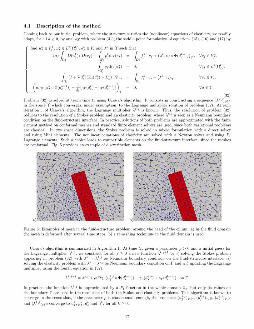
Lagrange elements. Such a choice leads to compatible elements on the fluid-structure interface, since the meshesare conformal. Fig. 5 provides an example of discretization mesh.

a) b)

Figure 5: Examples of mesh in the fluid-structure problem, around the head of the cilium. a) in the fluid domainthe mesh is deformed after several time steps. b) a remeshing technique in the fluid domain is used.

Uzawa’s algorithm is summarized in Algorithm 1. At time tk, given a parameter ρ > 0 and a initial guess forthe Lagrange multiplier λk,0, we construct for all j ≥ 0 a new function λk,j+1 by i) solving the Stokes problemappearing in problem (32) with λk = λk,j as Neumann boundary condition on the fluid-structure interface, ii)solving the elasticity problem with λk = λk,j as Neumann boundary condition on Γ and iii) updating the Lagrangemultiplier using the fourth equation in (32):

λk,j+1 = λk,j + ρ(δtγΓ(uk,jf Φ(dk−1s ))− γΓ(dk,js ) + γΓ(dk−1

s )), on Γ.

In practice, the function λk,j is approximated by a P1 function in the whole domain Ωs, but only its values onthe boundary Γ are used in the resolution of both the Stokes and elasticity problems. This algorithm is known toconverge in the sense that, if the parameter ρ is chosen small enough, the sequences (uk,jf )j∈N, (pk,jf )j∈N, (dk,js )j∈Nand (λk,j)j∈N converge to ukf , pkf , dks and λk, for all k ≥ 0.

17

Algorithm 1 Resolution of problem (32) at time tk (Uzawa’s algorithm).

Choose a parameter ρ and an initial guess λk,0 for the Lagrange multiplier.j = 0.while convergence criteria are not satisfied do

Compute the solution of the fluid problem (uk,jf , pk,jf ), with λk = λk,j .

Compute the solution of the structure problem dk,js with λk = λk,j .Update the Lagrange multiplier:

λk,j+1 = λk,j + ρ(δtγΓ(uk,jf Φ(dk−1s ))− γΓ(dk,js ) + γΓ(dk−1

s )), on Γ.

Update the number of iterations j = j + 1.end while

Once Uzawa’s algorithm has converged, we recover the velocity of the fluid at time tk, ukf , and the pressure of

the fluid at time tk, pkf , both defined in the deformed domain Ωkf . We also obtain the displacement of the structure

at time tk, dks , expressed in the reference solid configuration Ωs. The Lagrange multiplier at time tk, λk, is alsoobtained in Ωs and is used at the next time step as an initialization for Uzawa’s algorithm. Besides, to go to thenext time step, we move the fluid and structure meshes using the displacement of the structure. The solid mesh attime tk+1 is directly obtained by moving the mesh representing the domain Ωs with the displacement of the structureat time tk. For the fluid domain, we can not use directly the fluid displacement since fluid recirculations may occurand it could lead to poor quality meshes. Then, we construct the deformation Φ(dks) which maps the reference fluiddomain Ωf to the deformed fluid domain at time tk+1, Ωk+1

f . For that purpose, we solve a problem of linearized

elasticity in the domain Ωkf with Dirichlet boundary conditions on the deformed fluid-structure interface Γk given

by the displacement of the structure dks :find dkf : Ωk

f → Rn such that

−div(σs(dkf )) = 0, in Ωk

f ,

dkf = dks Φ−1(dk−1s ), on Γk,

dkf = 0, on Γkf ,

(33)

where σs(dkf ) is the linearized elasticity stress tensor defined by (19). Thus, the deformation of the fluid domain is

given byΦ(dks) = Φ(dk−1

s ) + dkf , in Ωf .

The displacement of the fluid domain, dkf , obtained through this process is smoother than the real displacementof the fluid, since the operator of linearized elasticity extends the displacement of the structure from the interfaceΓk to the whole domain Ωk

f with a diffusion process. However, this regularization process is not enough when thedisplacement of the structure is large, in which case the fluid domain has to be remeshed. More particularly, theinterior of the deformed fluid domain is remeshed but we never modify the boundary, since we want the fluid meshand the solid mesh to be conformal at the interface Γ. The algorithm is summarized in Algorithm 2.

The results shown in the remaining of the present section have been obtained using the finite element softwaresFEniCS, see [45], and FreeFem++, see [46]. The remeshing of the fluid domain is done with the Mmg software,see [47].

4.2 Influence of the fluid viscosity

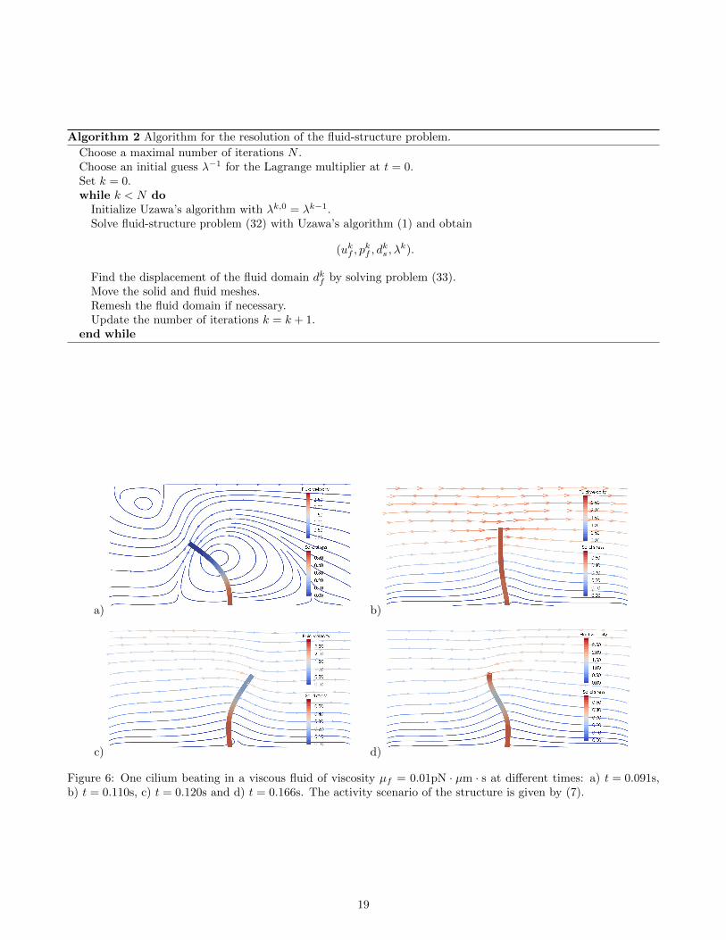
We start our numerical investigations with the study of the influence of the fluid viscosity on the fluid-structuresystem. In particular, we examine its effects on the deformations of the structure and on the displacements of thefluid. We consider the case of one cilium beating in a viscous fluid of viscosity µf with the activity scenario be givenby (7). The computational domain is a two-dimensional box of dimensions L1 = 20µm and L2 = 10µm. Initially,the cilium is represented as a vertical thin cylinder of length Lc = 6.5µm and radius rc = 0.2µm, anchored at thebottom. For the elasticity parameters of the structure we take Es = 106pN · µm−2 and νs = 0.49.

In Fig. 6, we show the result of the simulation, at different times, of the fluid-structure problem with a fluidviscosity µf = 0.01pN · µm−2 · s (ten times more viscous than water). Even though the internal activity of thecilium is imposed, the emerging beating pattern results from both the elasticity properties of the solid and thestrong coupling with the surrounding fluid. The fluid velocity is represented as streamlines and glyphs while, in the

18

Algorithm 2 Algorithm for the resolution of the fluid-structure problem.

Choose a maximal number of iterations N .Choose an initial guess λ−1 for the Lagrange multiplier at t = 0.Set k = 0.while k < N do

Initialize Uzawa’s algorithm with λk,0 = λk−1.Solve fluid-structure problem (32) with Uzawa’s algorithm (1) and obtain

(ukf , pkf , d

ks , λ

k).

Find the displacement of the fluid domain dkf by solving problem (33).Move the solid and fluid meshes.Remesh the fluid domain if necessary.Update the number of iterations k = k + 1.

end while

a) b)

c) d)

Figure 6: One cilium beating in a viscous fluid of viscosity µf = 0.01pN · µm · s at different times: a) t = 0.091s,b) t = 0.110s, c) t = 0.120s and d) t = 0.166s. The activity scenario of the structure is given by (7).

19

deformed solid domain, we plot at each point of the mesh the Frobenius norm of the Green-Lagrange strain tensor,defined in the reference configuration by√

E(ds(x)) : E(ds(x)), ∀x ∈ Ωs.

The Green-Lagrange strain tensor E(ds) measures the deformations of the solid material. It can also be seen asthe variations of the deformations of the structure compared to rigid deformations. In the present context, theFrobenius norm of the Green-Lagrange tensor gives us a general scalar criterion to observe the action of the fluidviscosity on the deformations of the structure.

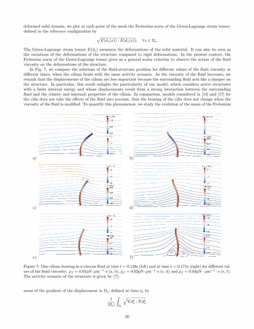
In Fig. 7, we compare the solutions of the fluid-structure problem for different values of the fluid viscosity atdifferent times, when the cilium beats with the same activity scenario. As the viscosity of the fluid increases, weremark that the displacements of the cilium are less important because the surrounding fluid acts like a damper onthe structure. In particular, this result enlights the particularity of our model, which considers active structureswith a finite internal energy and whose displacements result from a strong interaction between the surroundingfluid and the (elastic and internal) properties of the cilium. In comparison, models considered in [14] and [17] forthe cilia does not take the effects of the fluid into account, thus the beating of the cilia does not change when theviscosity of the fluid is modified. To quantify this phenomenon, we study the evolution of the mean of the Frobenius

a) b)

c) d)

e) f)

Figure 7: One cilium beating in a viscous fluid at time t = 0.128s (left) and at time t = 0.171s (right) for different val-ues of the fluid viscosity: µf = 0.01pN·µm−1 ·s (a, b), µf = 0.02pN·µm−1 ·s (c, d) and µf = 0.04pN · µm−1 · s (e, f).The activity scenario of the structure is given by (7).

norm of the gradient of the displacement in Ωs, defined at time tk by

1

|Ωs|

∫Ωs

√∇dks : ∇dks .

20

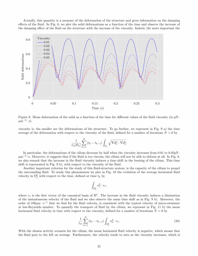
Actually, this quantity is a measure of the deformation of the structure and gives information on the dampingeffects of the fluid. In Fig. 8, we plot the solid deformations as a function of the time and observe the increase ofthe damping effect of the fluid on the structure with the increase of the viscosity. Indeed, the more important the

0 0.05 0.1 0.15 0.2 0.25 0.3

0

0.2

0.4

0.6

0.8

Time (s)

Soli

dd

efor

mati

ons

Viscosity0.010.020.030.040.05

Figure 8: Mean deformation of the solid as a function of the time for different values of the fluid viscosity (in pN ·µm−2 · s).

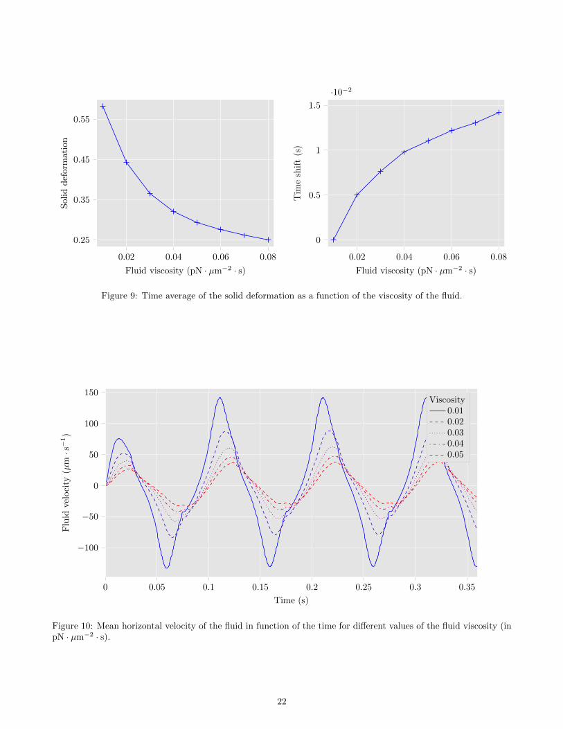
viscosity is, the smaller are the deformations of the structure. To go further, we represent in Fig. 9 a) the timeaverage of the deformation with respect to the viscosity of the fluid, defined for a number of iterations N > 0 by

1

tN |Ωs|

N∑k=1

(tk − tk−1)

∫Ωs

√∇dks : ∇dks .

In particular, the deformations of the cilium decrease by half when the viscosity increases from 0.01 to 0.05pN ·µm−2 · s. Moreover, it suggests that if the fluid is too viscous, the cilium will not be able to deform at all. In Fig. 8,we also remark that the increase in the fluid viscosity induces a time shift in the beating of the cilium. This timeshift is represented in Fig. 9 b), with respect to the viscosity of the fluid.

Another important criterion for the study of this fluid-structure system, is the capacity of the cilium to propelthe surrounding fluid. To study this phenomenon we plot in Fig. 10 the evolution of the average horizontal fluidvelocity in Ωk

f with respect to the time, defined at time tk by∫Ωk

f

ukf · e1,

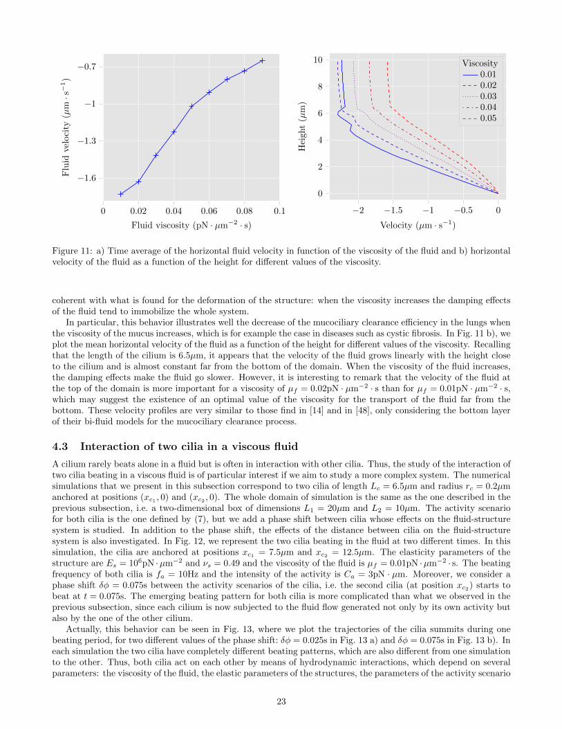
where e1 is the first vector of the canonical basis of R2. The increase in the fluid viscosity induces a diminutionof the instantaneous velocity of the fluid and we also observe the same time shift as in Fig. 9 b). Moreover, theorder of 100µm · s−1 that we find for the fluid velocity, is consistent with the typical velocity of micro-swimmerat low-Reynolds number. To quantify the transport of fluid by the cilium, we represent in Fig. 11 b) the meanhorizontal fluid velocity in time with respect to the viscosity, defined for a number of iterations N > 0 by

1

tN

N∑k=1

(tk − tk−1)

∫Ωk

f

ukf · e1. (34)

With the chosen activity scenario for the cilium, the mean horizontal fluid velocity is negative, which means thatthe fluid goes to the left on average. Furthermore, the velocity tends to zero as the viscosity increases, which is

21

0.02 0.04 0.06 0.08

0.25

0.35

0.45

0.55

Fluid viscosity (pN · µm−2 · s)

Soli

dd

efor

mati

on

0.02 0.04 0.06 0.08

0

0.5

1

1.5

·10−2

Fluid viscosity (pN · µm−2 · s)

Tim

esh

ift

(s)

Figure 9: Time average of the solid deformation as a function of the viscosity of the fluid.

0 0.05 0.1 0.15 0.2 0.25 0.3 0.35

−100

−50

0

50

100

150

Time (s)

Flu

idve

loci

ty(µ

m·s−

1)

Viscosity0.010.020.030.040.05

Figure 10: Mean horizontal velocity of the fluid in function of the time for different values of the fluid viscosity (inpN · µm−2 · s).

22

0 0.02 0.04 0.06 0.08 0.1

−0.7

−1

−1.3

−1.6

Fluid viscosity (pN · µm−2 · s)

Flu

idve

loci

ty(µ

m·s−

1)

−2 −1.5 −1 −0.5 0

0

2

4

6

8

10

Velocity (µm · s−1)

Hei

ght

(µm

)

Viscosity0.010.020.030.040.05

Figure 11: a) Time average of the horizontal fluid velocity in function of the viscosity of the fluid and b) horizontalvelocity of the fluid as a function of the height for different values of the viscosity.

coherent with what is found for the deformation of the structure: when the viscosity increases the damping effectsof the fluid tend to immobilize the whole system.

In particular, this behavior illustrates well the decrease of the mucociliary clearance efficiency in the lungs whenthe viscosity of the mucus increases, which is for example the case in diseases such as cystic fibrosis. In Fig. 11 b), weplot the mean horizontal velocity of the fluid as a function of the height for different values of the viscosity. Recallingthat the length of the cilium is 6.5µm, it appears that the velocity of the fluid grows linearly with the height closeto the cilium and is almost constant far from the bottom of the domain. When the viscosity of the fluid increases,the damping effects make the fluid go slower. However, it is interesting to remark that the velocity of the fluid atthe top of the domain is more important for a viscosity of µf = 0.02pN · µm−2 · s than for µf = 0.01pN · µm−2 · s,which may suggest the existence of an optimal value of the viscosity for the transport of the fluid far from thebottom. These velocity profiles are very similar to those find in [14] and in [48], only considering the bottom layerof their bi-fluid models for the mucociliary clearance process.

4.3 Interaction of two cilia in a viscous fluid

A cilium rarely beats alone in a fluid but is often in interaction with other cilia. Thus, the study of the interaction oftwo cilia beating in a viscous fluid is of particular interest if we aim to study a more complex system. The numericalsimulations that we present in this subsection correspond to two cilia of length Lc = 6.5µm and radius rc = 0.2µmanchored at positions (xc1 , 0) and (xc2 , 0). The whole domain of simulation is the same as the one described in theprevious subsection, i.e. a two-dimensional box of dimensions L1 = 20µm and L2 = 10µm. The activity scenariofor both cilia is the one defined by (7), but we add a phase shift between cilia whose effects on the fluid-structuresystem is studied. In addition to the phase shift, the effects of the distance between cilia on the fluid-structuresystem is also investigated. In Fig. 12, we represent the two cilia beating in the fluid at two different times. In thissimulation, the cilia are anchored at positions xc1 = 7.5µm and xc2 = 12.5µm. The elasticity parameters of thestructure are Es = 106pN ·µm−2 and νs = 0.49 and the viscosity of the fluid is µf = 0.01pN ·µm−2 · s. The beatingfrequency of both cilia is fa = 10Hz and the intensity of the activity is Ca = 3pN · µm. Moreover, we consider aphase shift δφ = 0.075s between the activity scenarios of the cilia, i.e. the second cilia (at position xc2) starts tobeat at t = 0.075s. The emerging beating pattern for both cilia is more complicated than what we observed in theprevious subsection, since each cilium is now subjected to the fluid flow generated not only by its own activity butalso by the one of the other cilium.

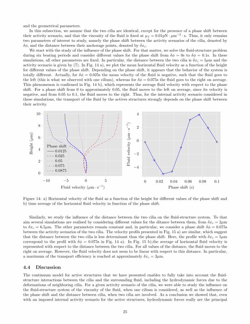
Actually, this behavior can be seen in Fig. 13, where we plot the trajectories of the cilia summits during onebeating period, for two different values of the phase shift: δφ = 0.025s in Fig. 13 a) and δφ = 0.075s in Fig. 13 b). Ineach simulation the two cilia have completely different beating patterns, which are also different from one simulationto the other. Thus, both cilia act on each other by means of hydrodynamic interactions, which depend on severalparameters: the viscosity of the fluid, the elastic parameters of the structures, the parameters of the activity scenario

23

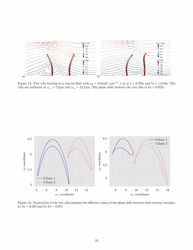
a) b)

Figure 12: Two cilia beating in a viscous fluid with µf = 0.01pN · µm−2 · s at a) t = 0.788s and b) t = 0.83s. Thecilia are anchored at xc1 = 7.5µm and xc2 = 12.5µm. The phase shift between the two cilia is δφ = 0.075s.

4 6 8 10 12 14

5

5.5

6

6.5

x1 coordinate

x2

coor

din

ate

Cilium 1Cilium 2

6 8 10 12 14 16

5

5.5

6

6.5

x1 coordinate

x2

coor

din

ate

Cilium 1Cilium 2

Figure 13: Trajectories of the two cilia summits for different values of the phase shift between their activity scenario:a) δφ = 0.025 and b) δφ = 0.075.

24

and the geometrical parameters.In this subsection, we assume that the two cilia are identical, except for the presence of a phase shift between

their activity scenario, and that the viscosity of the fluid is fixed at µf = 0.01pN · µm−2 · s. Thus, it only remainstwo parameters of interest to study, namely the phase shift between the activity scenarios of the cilia, denoted byδφ, and the distance between their anchorage points, denoted by δxc.

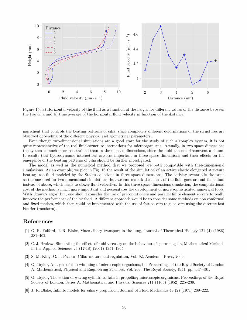
We start with the study of the influence of the phase shift. For that matter, we solve the fluid-structure problemduring six beating periods and consider different values for the phase shift from δφ = 0s to δφ = 0.1s. In thesesimulations, all other parameters are fixed. In particular, the distance between the two cilia is δxc = 5µm and theactivity scenario is given by (7). In Fig. 14 a), we plot the mean horizontal fluid velocity as a function of the heightfor different values of the phase shift. Depending on the phase shift, it appears that the behavior of the system istotally different. Actually, for δφ = 0.025s the mean velocity of the fluid is negative, such that the fluid goes tothe left (this is what we observed with one cilium), whereas for δφ = 0.075s the fluid goes to the right on average.This phenomenon is confirmed in Fig. 14 b), which represents the average fluid velocity with respect to the phaseshift. For a phase shift from 0 to approximately 0.05, the fluid moves to the left on average, since its velocity isnegative, and from 0.05 to 0.1, the fluid moves to the right. Thus, for the internal activity scenario considered inthese simulations, the transport of the fluid by the actives structures strongly depends on the phase shift betweentheir activity.

−10 −5 0 5

0

2

4

6

8

10

Fluid velocity (µm · s−1)

Hei

ght

(µm

)

Phase shift0.01250.0250.050.0750.0875

0 0.02 0.04 0.06 0.08 0.1

−4

−2

0

2

4

Phase shift (s)

Flu

idve

loci

ty(µ

m·s−

1)

Figure 14: a) Horizontal velocity of the fluid as a function of the height for different values of the phase shift andb) time average of the horizontal fluid velocity in function of the phase shift.

Similarly, we study the influence of the distance between the two cilia on the fluid-structure system. To thataim several simulations are realised by considering different values for the ditance between them, from δxc = 2µmto δxc = 6.5µm. The other parameters remain constant and, in particular, we consider a phase shift δφ = 0.075sbetween the activity scenarios of the two cilia. The velocity profils presented in Fig. 15 a) are similar, which suggestthat the distance between the two cilia is less determinant than the phase shift. Here, the profile with δxc = 5µmcorrespond to the profil with δφ = 0.075s in Fig. 14 a). In Fig. 15 b),the average of horizontal fluid velocity isrepresented with respect to the distance between the two cilia. For all values of the distance, the fluid moves to theright on average. However, the fluid velocity does not seem to be linear with respect to this distance. In particular,a maximum of the transport efficiency is reached at approximately δxc = 3µm.

4.4 Discussion

The continuum model for active structures that we have presented enables to fully take into account the fluid-structure interactions between the cilia and the surrounding fluid, including the hydrodynamic forces due to thedeformations of neighboring cilia. For a given activity scenario of the cilia, we were able to study the influence onthe fluid-structure system of the viscosity of the fluid, when one cilium is considered, as well as the influence ofthe phase shift and the distance between cilia, when two cilia are involved. As a conclusion we showed that, evenwith an imposed internal activity scenario for the active structures, hydrodynamic forces really are the principal

25

0 2 4 6 8 10

0

2

4

6

8

10

Fluid velocity (µm · s−1)

Hei

ght

(µm

)Distance

23456

2 3 4 5 6

4

4.2

4.4

4.6

Distance (µm)

Flu

idve

loci

ty(µ

m·s−

1)

Figure 15: a) Horizontal velocity of the fluid as a function of the height for different values of the distance betweenthe two cilia and b) time average of the horizontal fluid velocity in function of the distance.

ingredient that controls the beating patterns of cilia, since completely different deformations of the structures areobserved depending of the different physical and geometrical parameters.

Even though two-dimensional simulations are a good start for the study of such a complex system, it is notquite representative of the real fluid-structure interactions for microorganisms. Actually, in two space dimensionsthe system is much more constrained than in three space dimensions, since the fluid can not circumvent a cilium.It results that hydrodynamic interactions are less important in three space dimensions and their effects on theemergence of the beating patterns of cilia should be further investigated.

The model as well as the numerical method that we proposed are both compatible with thee-dimensionalsimulations. As an example, we plot in Fig. 16 the result of the simulation of an active elastic elongated structurebeating in a fluid modeled by the Stokes equations in three space dimensions. The activity scenario is the sameas the one used for two-dimensional simulations, but we can remark that most of the fluid goes around the ciliuminstead of above, which leads to slower fluid velocities. In this three space dimensions simulation, the computationalcost of the method is much more important and necessitates the development of more sophisticated numerical tools.With Uzawa’s algorithm, one should consider the use of preconditioners and parallel finite element solvers to reallyimprove the performance of the method. A different approach would be to consider some methods on non conformaland fixed meshes, which then could be implemented with the use of fast solvers (e.g. solvers using the discrete fastFourier transform).

References

[1] G. R. Fulford, J. R. Blake, Muco-ciliary transport in the lung, Journal of Theoretical Biology 121 (4) (1986)381–402.

[2] C. J. Brokaw, Simulating the effects of fluid viscosity on the behaviour of sperm flagella, Mathematical Methodsin the Applied Sciences 24 (17-18) (2001) 1351–1365.

[3] S. M. King, G. J. Pazour, Cilia: motors and regulation, Vol. 92, Academic Press, 2009.

[4] G. Taylor, Analysis of the swimming of microscopic organisms, in: Proceedings of the Royal Society of LondonA: Mathematical, Physical and Engineering Sciences, Vol. 209, The Royal Society, 1951, pp. 447–461.

[5] G. Taylor, The action of waving cylindrical tails in propelling microscopic organisms, Proceedings of the RoyalSociety of London. Series A. Mathematical and Physical Sciences 211 (1105) (1952) 225–239.

[6] J. R. Blake, Infinite models for ciliary propulsion, Journal of Fluid Mechanics 49 (2) (1971) 209–222.

26

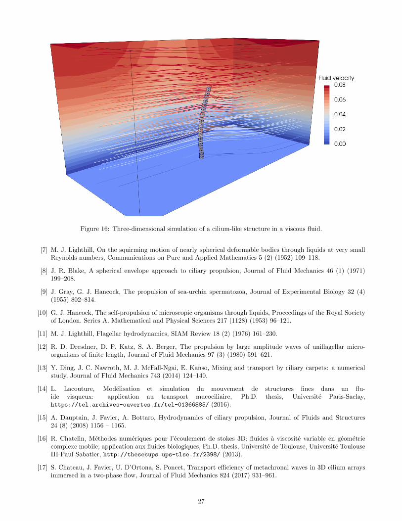
Figure 16: Three-dimensional simulation of a cilium-like structure in a viscous fluid.

[7] M. J. Lighthill, On the squirming motion of nearly spherical deformable bodies through liquids at very smallReynolds numbers, Communications on Pure and Applied Mathematics 5 (2) (1952) 109–118.

[8] J. R. Blake, A spherical envelope approach to ciliary propulsion, Journal of Fluid Mechanics 46 (1) (1971)199–208.

[9] J. Gray, G. J. Hancock, The propulsion of sea-urchin spermatozoa, Journal of Experimental Biology 32 (4)(1955) 802–814.

[10] G. J. Hancock, The self-propulsion of microscopic organisms through liquids, Proceedings of the Royal Societyof London. Series A. Mathematical and Physical Sciences 217 (1128) (1953) 96–121.

[11] M. J. Lighthill, Flagellar hydrodynamics, SIAM Review 18 (2) (1976) 161–230.

[12] R. D. Dresdner, D. F. Katz, S. A. Berger, The propulsion by large amplitude waves of uniflagellar micro-organisms of finite length, Journal of Fluid Mechanics 97 (3) (1980) 591–621.

[13] Y. Ding, J. C. Nawroth, M. J. McFall-Ngai, E. Kanso, Mixing and transport by ciliary carpets: a numericalstudy, Journal of Fluid Mechanics 743 (2014) 124–140.

[14] L. Lacouture, Modelisation et simulation du mouvement de structures fines dans un flu-ide visqueux: application au transport mucociliaire, Ph.D. thesis, Universite Paris-Saclay,https://tel.archives-ouvertes.fr/tel-01366885/ (2016).

[15] A. Dauptain, J. Favier, A. Bottaro, Hydrodynamics of ciliary propulsion, Journal of Fluids and Structures24 (8) (2008) 1156 – 1165.

[16] R. Chatelin, Methodes numeriques pour l’ecoulement de stokes 3D: fluides a viscosite variable en geometriecomplexe mobile; application aux fluides biologiques, Ph.D. thesis, Universite de Toulouse, Universite ToulouseIII-Paul Sabatier, http://thesesups.ups-tlse.fr/2398/ (2013).

[17] S. Chateau, J. Favier, U. D’Ortona, S. Poncet, Transport efficiency of metachronal waves in 3D cilium arraysimmersed in a two-phase flow, Journal of Fluid Mechanics 824 (2017) 931–961.

27

[18] K. E. Machin, Wave propagation along flagella, Journal of Experimental Biology 35 (4) (1958) 796–806.

[19] C. J. Brokaw, Bend propagation along flagella, Nature 209 (5019) (1966) 161–163.

[20] J. Lubliner, J. J. Blum, Model for bend propagation in flagella, Journal of Theoretical Biology 31 (1) (1971)1 – 24.

[21] C. J. Brokaw, Computer simulation of flagellar movement: I. demonstration of stable bend propagation andbend initiation by the sliding filament model, Biophysical Journal 12 (5) (1972) 564–586.

[22] M. Hines, J. J. Blum, Bend propagation in flagella. I. Derivation of equations of motion and their simulation,Biophysical Journal 23 (1) (1978) 41–57.

[23] C. J. Brokaw, Computer simulation of flagellar movement. VI. Simple curvature-controlled models are incom-pletely specified, Biophysical Journal 48 (4) (1985) 633–642.

[24] K. E. Machin, The control and synchronization of flagellar movement, Proceedings of the Royal Society ofLondon. Series B. Biological Sciences 158 (970) (1963) 88–104.

[25] C. J. Brokaw, Computer simulation of flagellar movement IX. Oscillation and symmetry breaking in a modelfor short flagella and nodal cilia, Cell Motility and the Cytoskeleton 60 (1) (2005) 35–47.

[26] M. Murase, The dynamics of cellular motility, John Wiley and Sons, 1992.

[27] R. H. Dillon, L. J. Fauci, An integrative model of internal axoneme mechanics and external fluid dynamics inciliary beating, Journal of Theoretical Biology 207 (3) (2000) 415–430.

[28] R. H. Dillon, L. J. Fauci, C. Omoto, Mathematical modeling of axoneme mechanics and fluid dynamics in ciliaryand sperm motility, Dynamics of Continuous Discrete and Impulsive Systems Series A 10 (2003) 745–758.

[29] X. Yang, R. H. Dillon, L. J. Fauci, An integrative computational model of multiciliary beating, Bulletin ofMathematical Biology 70 (4) (2008) 1192–1215.

[30] S. Lukens, X. Yang, L. J. Fauci, Using Lagrangian coherent structures to analyze fluid mixing by cilia, Chaos:An Interdisciplinary Journal of Nonlinear Science 20 (1) (2010) 017511.

[31] S. Gueron, K. Levit-Gurevich, A three–dimensional model for ciliary motion based on the internal 9+2 struc-ture, Proceedings of the Royal Society of London. Series B: Biological Sciences 268 (1467) (2001) 599–607.

[32] S. M. Mitran, Metachronal wave formation in a model of pulmonary cilia, Computers and Structures 85 (11)(2007) 763–774.

[33] D. Ambrosi, S. Pezzuto, Active stress vs. active strain in mechanobiology: constitutive issues, Journal ofElasticity 107 (2) (2012) 199–212.

[34] N. P. Smith, A computational study of the interaction between coronary blood flow and myocardial mechanics,Physiological Measurement 25 (4) (2004) 863.

[35] A. V. Panfilov, R. H. Keldermann, M. P. Nash, Self-organized pacemakers in a coupled reaction-diffusion-mechanics system, Physical Review Letters 95 (25) (2005) 258104.

[36] D. K. Bogen, S. A. Rabinowitz, A. Needleman, T. A. Mcmahon, W. H. Abelmann, An analysis of the mechanicaldisadvantage of myocardial infarction in the canine left ventricle, Circulation Research 47 (5) (1980) 728–741.

[37] S. Pezzuto, D. Ambrosi, A. Quarteroni, An orthotropic active–strain model for the myocardium mechanics andits numerical approximation, European Journal of Mechanics-A/Solids 48 (2014) 83–96.

[38] Y. Payan, J. Ohayon, Biomechanics of living organs: hyperelastic constitutive laws for finite element modeling,Academic Press, 2017.

[39] M. E. J. Holwill, P. Satir, Generation of propulsive forces by cilia and flagella, Cytomechanics (1987) 120–130.

[40] E. M. Purcell, Life at low Reynolds number, American Journal of Physics 45 (1) (1977) 3–11.

28

[41] F. Vergnet, Structures actives dans un fluide visqueux : modelisation, analyse mathematique et simulationsnumeriques, Ph.D. thesis, Universite Paris-Saclay, https://tel.archives-ouvertes.fr/tel-02194265/

(2019).

[42] M. E. Bogovski, Solution of the first boundary value problem for an equation of continuity of an incompressiblemedium, Doklady Akademii Nauk SSSR 248 (5) (1979) 10371040.

[43] F. Brezzi, On the existence, uniqueness and approximation of saddle-point problems arising from Lagrangianmultipliers, Revue Francaise d’Automatique, Informatique, Recherche Operationnelle. Analyse Numerique8 (R2) (1974) 129–151.

[44] F. Boyer, P. Fabrie, Elements d’analyse pour l’etude de quelques modeles d’ecoulements de fluides visqueuxincompressibles, Vol. 52, Springer Science and Business Media, 2005.

[45] A. Logg, K.-A. Mardal, G. Wells, Automated solution of differential equations by the finite element method:The FEniCS book, Vol. 84, Springer Science and Business Media, 2012.

[46] F. Hecht, New development in FreeFem++, Journal of Numerical Mathematics 20 (3-4) (2012) 251–266.

[47] C. Dapogny, C. Dobrzynski, P. Frey, Three-dimensional adaptive domain remeshing, implicit domain meshing,and applications to free and moving boundary problems, Journal of Computational Physics 262 (2014) 358–378.

[48] D. J. Smith, E. A. Gaffney, J. R. Blake, Modelling mucociliary clearance, Respiratory Physiology and Neuro-biology 163 (1) (2008) 178–188.

29