A Constructive Formalisation of Semi-algebraic Sets and ...

HAL Id: hal-01643919https://hal.inria.fr/hal-01643919

Submitted on 21 Nov 2017

HAL is a multi-disciplinary open accessarchive for the deposit and dissemination of sci-entific research documents, whether they are pub-lished or not. The documents may come fromteaching and research institutions in France orabroad, or from public or private research centers.

L’archive ouverte pluridisciplinaire HAL, estdestinée au dépôt et à la diffusion de documentsscientifiques de niveau recherche, publiés ou non,émanant des établissements d’enseignement et derecherche français ou étrangers, des laboratoirespublics ou privés.

A Constructive Formalisation of Semi-algebraic Sets andFunctionsBoris Djalal

To cite this version:Boris Djalal. A Constructive Formalisation of Semi-algebraic Sets and Functions. CPP 2018 - Pro-ceedings of the 7th ACM SIGPLAN International Conference on Certified Programs and Proofs, Jan2018, Los Angeles, California, United States. pp.240-251. �hal-01643919�

https://hal.inria.fr/hal-01643919

https://hal.archives-ouvertes.fr

12345678910111213141516171819202122232425262728293031323334353637383940414243444546474849505152535455

5657585960616263646566676869707172737475767778798081828384858687888990919293949596979899100101102103104105106107108109110

A Constructive Formalisation of Semi-Algebraic Setsand Functions

Boris DjalalInria Sophia Antipolis – Méditerranée, France

[email protected]

AbstractSemi-algebraic sets and semi-algebraic functions are essen-tial to specify and certify cylindrical algebraic decompositionalgorithms. We formally define in Coq the base operationson semi-algebraic sets and functions using embedded first-order formulae over the language of real closed fields, andwe prove the correctness of their geometrical interpretation.In doing so, we exploit a previous formalisation of quantifierelimination on such embedded formulae to guarantee thedecidability of several first-order properties and keep ourdevelopment constructive. We also exploit it to formaliseformulae substitution without having to handle bound vari-ables.

Keywords Formalisation of Mathematics, Semi-AlgebraicSets, Semi-Algebraic Functions, Coq, Quantifier Elimination,Real Algebraic Geometry, Substitution

1 IntroductionFirst-order formulae over real closed fields, which can ex-press a wide range of problems (polynomial optimisation,topologically reliable algebraic curve display, terminationproof of term-rewriting systems) [5] are decidable. Quantifierelimination, that consists in finding a logically equivalentformula without quantifiers, is the keystone of the decisionprocedures for first-order formulae presented in the litera-ture [5]. The first quantifier elimination algorithm [24] hascomplexity a tower of exponents of height linear in the num-ber of variables [2]. The cylindrical algebraic decomposition(abbreviated by CAD from now on) was invented by GeorgeE. Collins to eliminate quantifiers with a better complexitythan Tarski’s original algorithm [1, 3]: the complexity re-duces to a double exponential in the number of quantifiers.The expression “CAD” denotes two different notions: thealgorithm and its output. In this paper, we call “CAD” a parti-tion of the geometric space into semi-algebraic (abbreviatedby S.A. from now on) sets, which satisfies some additionalproperties as explained in Sect. 4.1. We call “CAD algorithm”any algorithm that returns such a partition. Moreover, CADalgorithms help to answer questions about central objectsin real algebraic geometry, S.A. sets. For example: how tocompute sample points of a given nonempty S.A. set or the

CPP’18, January 07–08, 2018, Los Angeles, LA, USA2018.

number of points of a S.A. set, decide whether a S.A. set isopen, closed or bounded, determine the connected compo-nents of a S.A. set [2].To work on the correctness proof of a given CAD algo-

rithm, one firstly needs to tackle the two following problems:formalise what constitutes a CAD output, then formalisewhat constitutes a CAD algorithm.

In the present work, we formalise two key concepts re-quired to formalise what constitutes the output of aCAD, S.A.sets and S.A. functions, while exploiting a previous quantifierelimination formalised by Cohen andMahboubi [9]. DefiningS.A. sets and S.A. functions brings us to solve intermediaryproblems to represent such objects in Coq.In Sect. 2, we introduce preliminary notions required by

the CAD, by S.A. sets and by S.A. functions.Firstly, in Sect. 2.1, we briefly clarify what is a first order

formula on a real closed field. On top of first-order formu-lae, we define sets of free variables in Sect. 2.2. This en-ables us to build the type of formulae with free variablesin {X0, · · · ,Xn−1} in Sect. 2.4. We remind what is quantifierelimination and how we use the one fromMathematicalComponents [21] in Sect. 2.3.In particular, we use it in Sect. 3 to define the logical

equivalence relation on such formulae in a decidable way(to keep our development constructive).

We describe the construction of the type of S.A. sets inSect. 4. Firstly, we define the CAD and explain why we needthe S.A. set concept in Sect. 4.1. Secondly, we formalise S.A.sets in Sect. 4.2 through a quotient structure by combiningresults on formulae. We prove that two S.A. sets are equal if,and only if, they contain the same elements. We then equipS.A. sets with a lattice structure.

In Sect. 5, we describe our formalisation of S.A. functions,whose graphs are S.A. sets. This formalisation requires toexpress functionality and totality of S.A. graphs in a decidableway (to keep our development constructive). We achievethis by constructing tailor-made reified formulae expressingfunctionality and totality and by proving their correctness,similarly to the reification technique presented in [16, 20, 23].These constructions rely on the substitution in formulae. Wedo not define the substitution in the usual way, as in [13, 14].Instead, we simplify the definition and specification of thesubstitution in formulae by exploiting quantifier elimination,in Sect. 6.1.

1

111112113114115116117118119120121122123124125126127128129130131132133134135136137138139140141142143144145146147148149150151152153154155156157158159160161162163164165

CPP’18, January 07–08, 2018, Los Angeles, LA, USA Boris Djalal

166

167

168

169

170

171

172

173

174

175

176

177

178

179

180

181

182

183

184

185

186

187

188

189

190

191

192

193

194

195

196

197

198

199

200

201

202

203

204

205

206

207

208

209

210

211

212

213

214

215

216

217

218

219

220

Using the same methodology as for functionality and to-tality, we show how to formalise the composition of twoS.A. functions in Sect. 7 and the continuity of a S.A. functionin Sect. 8. The latter turns out to be more difficult and weprovide an incomplete proof of correctness.

In the present paper, we present modified snippets of ourcode available at https://github.com/math-comp/cad.

2 Preliminary NotionsIn this section, we briefly remind (2.1) what is quantifierelimination (2.3) in the Mathematical Components set-tings; we present our contributions about free variables (2.2)and formulae (2.4) (3).

2.1 First-Order Formulae over Real Closed FieldsIn this paper, we use first-order formulae over real closedfields to formalise S.A. sets. We now clarify these two notions.

One definition is that a real closed field is an ordered fieldthat has no ordered algebraic extension [7]. In particular, it isequipped with the arithmetic operations (addition, negation,multiplication and thus exponentiation with a natural num-ber) and with comparison. For example, the real numbersand the real algebraic number are real closed fields. To keepthe analogy with real numbers, we denote a real closed fieldby R. However, in all our work, we do no suppose that R isarchimedean, whereas the real numbers is archimedean.We use operations on R to define terms and first-order

formulae. A term over R is a variable Xi , i ∈ N or else aformal operation over terms. Formal arithmetic operationsare: addition, multiplication, exponentiation, and negation. Aformula over a field R is defined inductively as a formal com-parison of two terms or else as a formal logical operation onformulae. A formal logical operation is either a formal logicalconnective (and, or, implication, negation) or a formal quan-tification of a formula over a variable — quantifying over analready bounded variable or missing variable is thus allowed.For example, ∃X0∃X0X0 = 0, ∃X0X1 = 0 and ∃X2∃X3((X2 + X3 − X0 = 0)∧( 13X2X3 − X1)∧(X2 < X3)

)are valid for-

mulae over R.In our work, we exploit a previous formalisation of real

closed fields and first-order formulae fromMathematicalComponents.

2.2 Free VariablesThe free variables of a first-order formula are the variablesthat are not bound by a quantifier. They are the dimensions ofRn that matter in the geometric interpretation of the formula,so they play a central role in S.A. sets over Rn as describedin Sect. 2.4. We compute the free variables recursively as fol-lows: the free variables of the termXi is the set {Xi }; the freevariables of a quantification formula of the form Q

Xi ϕ,

Q

∈

{∀,∃}, are the free variables of the subformula ϕ minus Xi .In all other cases, the free variables of a formula is the union

of the free variables of its subformulae. For example, the freevariables of ∃X2∃X3

((X2 + X3 − X0 = 0)∧( 13X2X3 − X1)∧

(X2 < X3))is the set {X0}.

In Coq, finite sets can be represented by sequences with-out duplicates. With this representation, In our formalisation,we use the appropriate, higher level, notion of finite set fromMathematical Components instead of sequences. It allowsus to work with the Coq equality (=) on finite sets, instead ofthe extensional equivalence (=i in Coq) on sequences of vari-ables. Moreover, we automatically get a decidable equality onsets of variables, because the equality on natural numbers isdecidable. We use this to keep our development constructive(but we do not run any decision procedure).

2.3 Semantics of First-Order Formulae andQuantifier Elimination

Terms and formulae are geometrically interpreted respec-tively as elements of R and Coq first-order formulae. Theinterpretation has already been defined by Cohen [9] andcorresponds to two functions eval and holds, which take anenvironment e to give values to free variables and respec-tively output an element of R and an element of Prop. Anopen formula with free variables in X0, · · · ,Xn−1 can beviewed as a predicate on Rn , i.e. a subset of Rn .

In this work we exploit the formalisation of a quantifierelimination procedure from a previous work by Cohen andMahboubi [9], which applies to formulae over a real closedfield.Firstly we use the existing decision procedure, rcf_sat,

to decide whether a given first-order formula f is true ina given environment e. It is expressed b ythe expressionrcf_sat e f (with type bool) in Coq where e assignes val-ues to all free variables of f. When f is closed, this is writtenas rcf_sat [::] f. In particular, we use this decision pro-cedure to define the decidable logical equivalence of twofirst-order formulae in Sect. 3.Secondly, we use the quantifier elimination procedure

in Sect. 6.1. A quantifier elimination procedure returns anequivalent quantifier-free formula. However, the existingquantifier elimination procedure, quantifier_elim, is notspecified enough to guarantee that no free variable is in-troduced. Based on quantifier_elim, we define anotherone, qf_elim, which does not introduce new free variable,as follows. In Coq, we consider an input formula f and thequantifier-free equivalent g given by quantifier_elim. Theformula g may introduce new free variables from the vari-ables set formula_fv g `\` formula_fv f. The instanti-ation of these extra variables does not affect f. Thus, theinstantiation of these extra variables in g returns a formulaequivalent to g. We choose to instantiate these variables ing with 0. We define quantifier_elim in Coq. We formallyprove that the resulting formula is equivalent to f, that it

2

221222223224225226227228229230231232233234235236237238239240241242243244245246247248249250251252253254255256257258259260261262263264265266267268269270271272273274275

A Constructive Formalisation of Semi-Algebraic Sets and Functions CPP’18, January 07–08, 2018, Los Angeles, LA, USA

276

277

278

279

280

281

282

283

284

285

286

287

288

289

290

291

292

293

294

295

296

297

298

299

300

301

302

303

304

305

306

307

308

309

310

311

312

313

314

315

316

317

318

319

320

321

322

323

324

325

326

327

328

329

330

is quantifier-free, and the following statement that its freevariables are among those of f:Lemma qf_elim_fv (f : formula R) :

formula_fv (qf_elim f) <= formula_fv f.

where <= denotes the subset relation.

2.4 Formulae with less than n Free VariablesS.A. sets of Rn involve a finite number of variables amongX0, · · · ,Xn−1. Since we can find an equivalent formula with-out bound variables (Sect. 2.3), we consider formulae withfree variables among X0, · · · ,Xn−1, which we denote byFn = {φ ∈ F | freevar(φ) ⊆ {X0, · · · ,Xn−1}}. In Coq, we de-note R by R and n by n and we encode X0, · · · ,Xn−1 by thevariables 'X_0, . . . ,'X_(n - 1) and we define the decidablepredicate freevar(φ) ⊆ {X0, · · · ,Xn−1} by:Definition nvar (n : nat) :=fun (f : formula R) => formula_fv f <= mnfset O n.where mnfset O n is the set of natural numbers rangingfrom 0 to n − 1. The set Fn is then formalised by:Record formulan := MkFormulan

{

underlying_f : formula R ;

_ : nvar underlying_f

}.

Notation "'{formula_' n R }" := (formulan R n).

Formulae over R with less than n free variables inherit thechoice type structure from F . Given any inhabitated pred-icate (inhabitated decidable property) over a choice typestructure, one can choose a witness of that predicate. Wechoose the same witness for any logically equivalent prop-erty. See the Mathematical Components book [21] formore information on choice types.We automatically cast elements of Fn to elements of F

using the Coq implicit coercion mechanism:Coercion underlying_f : formulan >−> formula.The theorems which apply to F also apply to Fn , by coer-cion. For example, the formula constructor And expects twoelements of F , yet we can apply it to two elements f and gof Fn and get the element f /\ g of F .

In our example, f /\ g still has n variables. We prove thisin Coq:Lemma and_formulan (f g : {formula_n R}) : nvar n (f /\ g)%oT.where oT makes interpret the symbol /\ in the scope offormulae. This situation is similar to tuples inMathemati-cal Components. Tuples are sequences with a given length.When we concatenate two tuples, we obtain a sequencewhose length is the sum of the lengths. InMathematicalComponents, this piece of information is recovered auto-matically by declaring a canonical solution [21].

In a similar way, we automatically recover the piece ofinformation about f /\ g by declaring and_formulan as acanonical solution:

Canonical Structure formulan_and f g :=

MkFormulan (and_formulan f g).

Then, the system is able to build the proof of nvar underlying_f

on the fly for any two specific values f and g, and lift f /\ gto Fn . We implement similar solutions for other operations.

2.5 Decidable Equivalence Relation over Formulaewith less than n Free Variables

To define S.A. sets in (see Sect. 4), we need to define thelogical equivalence relation over Fn .In all this Sect., we suppose that we have an equivalence

relation equivf over F (see Sect. 3) such that its restrictionto Fn is the logical equivalence relation over Fn . We showhow to formalise this restriction in a more general settings.Since we can use elements of Fn in place for elements

of F , we can see equivf as an equivalence relation onFn . In Coq, we define a new relation on {formula_n R}by restricting equivf to formulae with free variables inX0, · · · ,Xn−1; we then prove that this restriction is an equiv-alence relation.Instead of directly proving that the subrelation induced

by equivf on formula_n F is also an equivalence relation,we generalise this construction over the types formula andformula_n R: any equivalence relation on a type T inducesan equivalence relation sub_r on any subtype of T (subtypestructures are explained in theMathematical Componentsbook [21]). We define sub_r in Coq by:

Variables (T : eqType) (P : pred T) (sT : subType P) (r : equiv_rel T).Definition sub_r (x y : sT) := r (val x) (val y).

We bring down reflexivity (sub_r_refl), symmetry (sub_r_sym)and transitivity (sub_r_trans) of sub_r to the reflexivity, sym-metry and transitivity of equiv_rel, respectively. This way,we formally prove these three properties for the subrelationsub_r. We make the equivalence structure of the subrela-tion a canonical structure, so that this structure is recoveredautomatically by the system:

Canonical sub_r_equiv :=

EquivRel sub_r sub_r_refl sub_r_sym sub_r_trans.

Our generic canonical solution takes the proof that the broaderrelation is an equivalence relation and the desired subtype,then automatically builds the equivalence relation inducedon the subtype.We apply this generic construction to define the logical equiv-alence sub_equivf on Fn , in Coq:

Definition sub_equivf :=@sub_r _ _ [subType of {formula_n R}] equivf_equiv.

3

331332333334335336337338339340341342343344345346347348349350351352353354355356357358359360361362363364365366367368369370371372373374375376377378379380381382383384385


386

387

388

389

390

391

392

393

394

395

396

397

398

399

400

401

402

403

404

405

406

407

408

409

410

411

412

413

414

415

416

417

418

419

420

421

422

423

424

425

426

427

428

429

430

431

432

433

434

435

436

437

438

439

440

3 First Reification case for the EquivalenceRelation over Formulae

In this section, we define a logical equivalence relation onformulae, such that its restriction to Fn (see Sect. 2.5) is adecidable equivalence. We show how to use reification toexpress this relation in a decidable way.

Let ϕ andψ denote two formulae. We consider the follow-ing relation: ϕ and ψ are equivalent if they evaluate to thesame truth-value in all environments of size n (any free vari-able Xi with n < i is assigned to the default value 0). In Coq,this can be expressed by the following property of type Prop:forall (e : n.-tuple F), holds e f <-> holds e g,where e is a sequence of size n (in other words e is a tupleof size n, denoted n.-tuple F). To write a decidable ver-sion of this property, we first need to express it through thespecific formula type expected by rcf_sat (this is called reifi-cation), then evaluate its boolean truth-value with rcf_sat.We firstly remark that holds e f <-> holds e g is thedefinition of holds e (f <==> g) where <==> is the equiv-alence in the language of real closed fields. We are thus ableto express the connector <-> on Prop in the language of realclosed fields. (In our code, the constant <==> is not directlypart of the language, but we define it in terms of ==> and /\.)

To complete the reification, we push quantification over einward, so that quantification over e is replaced by n quan-tifications over variables. The latter quantifications are partof the targeted first-order language. A reified version of theproperty above thus has the form ∀X0 · · · ∀Xn−1 ϕ ⇐⇒ ψ ,in Coq:

nquantify O n Forall (f <==> g)

Listing 1.

where the function nquantify i n

Qprefixes any formulawith the block quantification Q

Xi · · ·

Q

Xi+n−1 from the in-dex i up to the index i + n − 1 with Qbeing one of the quan-tifiers ∀ or ∃. We illustrate the working of nquantify on thefollowing example. The application of nquantify 3 2 Forall

on the formula ∃X5 (X5 = X3 ∨ X5 = X4)∧X3 ≤ X5 ∧ X4 ≤ X5outputs the formula ∀X3∀X4∃X5 (X5 = X3 ∨ X5 = X4)∧X3 ≤ X5 ∧ X4 ≤ X5. The resulting formula is closed (we re-mark that it means that any numbers pair (X3,X4) have amaximum X5). This formula (Listing 1) is called a reifiedformula according to the reification techniques presented inother works [16, 20, 23]. Since it is a first-order formula inthe expected type, we can apply rcf_sat on it. We evaluateit in the empty environment (which assigns any free vari-able to the default assignment value 0). In Coq, a decidableversion of our equivalence relation is expressed by:

Definition equivf (f g : formula R) :=rcf_sat [::] (nquantify O n Forall (f <==> g)).

Our decidable version is used for the only sake of con-structivity of our development, we do not use it to make

computations; contrary to other works [16, 20, 23], wherethe reification is used to compute decision procedures toreplace proof steps with computations (reflection). The sec-ond point of comparison with these works [16, 20, 23] isthat we do not need a tactic to automatically generate reifiedformulae.

We prove in Coq that equivf is reflexive, symmetric andtransitive. We make the equivalence structure of equivf acanonical structure.The certification of equivf is a consequence of the certi-

fications of rcf_sat and nquantify. We certify the univer-sal block quantification as follows. Evaluating the formulanquantify a k Forall f in an environment is not affectedby the values associated by this environment to variables Xifora ≤ i; variablesXi fora ≤ i < a+k are bound by the blockquantification and variables Xi or a + k ≤ i are evaluated to0 by definition of our block quantification. Thus, we considerenvironments e whose size is exactly a. We formally prove:Lemma nforallP (k : nat) (e : seq R) (f : formula R) :forall v : k.−tuple R, holds (e ++ v) f<−> holds e (nquantify (size e) k Forall f).where ++ denotes the sequences concatenation. This lemmastates that the evaluation of the universal block quantifica-tion over f in the environment e is true if, and only if, theevaluation of f is true in any environment e ++ v where vis a sequence of length k.Similarly, we formally certify the existential block quan-

tification:

Lemma nexistsP (k : nat) (e : seq R) (f : formula R) :exists v : k.−tuple R, holds (e ++ v) f<−> holds e (nquantify (size e) k Exists f).

4 Formalisation of Semi-Algebraic SetsA S.A. set of Rn is the set that realizes a formula of Fn . It is asubset of Fn . However, numerous elements of Fn , some ofwhich are quantifier-free, realize the same S.A. set. Testingfor the equality of two S.A. sets amounts to testing for theequivalence of two elements of Fn under any environment.We firstly explain why we need the S.A. set concept by

introducing CAD in Sect. 4.1. Then, in Sect. 4.2, we explainhow we build S.A. sets as the mathematical quotient of Fnby exploiting the logical equivalence relation over Fn .

4.1 Cylindrical Algebraic Decomposition DefinitionA CAD of Rn is a partition (Cj )1≤j≤c (c ∈ N∗) of Rn intoconnected S.A. sets Ci , called cells, satisfying the followingproperty: for any canonical projection π : Rn −→ Rn−k(with k ≤ n), consisting in forgetting the last k coordinates,and for any cells Ci and Cj , one have π (Ci ) = π (Cj ) or elseπ (Ci ) ∩ π (Cj ) = ∅. The images by π of the cells define aCAD of Rn−k (note that S.A. sets are stable by the canonical

4

441442443444445446447448449450451452453454455456457458459460461462463464465466467468469470471472473474475476477478479480481482483484485486487488489490491492493494495


496

497

498

499

500

501

502

503

504

505

506

507

508

509

510

511

512

513

514

515

516

517

518

519

520

521

522

523

524

525

526

527

528

529

530

531

532

533

534

535

536

537

538

539

540

541

542

543

544

545

546

547

548

549

550

−∞ ∞0

(a) CAD of the line R

−∞ ∞0

(b) CAD of the line R

Figure 1

1

2

3

4

5

6

Figure 2. CAD of the plane R2

projections) [2, 26]. When n = 1, the above definition ofCAD amounts to.Another view of the CAD output is a bottom-up view,

which starts by defining the CAD in dimension 1, then 2,etc. It is the original approach of Collins [5]. In dimension1, a CAD is a finite partition of R into intervals (includ-ing singletons). For example,

{]−∞, 0[, [0,∞[

}(Fig. 1a) and{

[−∞, 0], [0], [0,∞]}(Fig. 1b) are two valid CAD of R. Then,

one defines inductively a CAD of Rn+1 by using a CAD ofRn . A cell in the CAD of Rn+1 is defined above a cell of thegiven CAD of Rn by providing one or two delimiting contin-uous S.A. functions; we define S.A. functions in Sect. 5. Forexample, the CAD (Fig. 2) defined by the cells:• {(x ,y) ∈ F 2 |x < 0, 0 < y} 1

• {(x ,y) ∈ F 2 |x < 0,y ≤ 0} 2

• {(x ,y) ∈ F 2 |0 ≤ x ,y <√x − 1} 3

• {(x ,y) ∈ F 2 |0 ≤ x ,y =√x − 1} 4

• {(x ,y) ∈ F 2 |0 ≤ x ,√x − 1 < y ≤ 2 − x2} 5

• {(x ,y) ∈ F 2 |0 ≤ x , 2 − x2 < y} 6is a valid CAD of R2 built on top of the CAD of Fig. 1a.Both views are based on continuous S.A. functions, be-

cause S.A. set connectedness (in the higher level view) isequivalent to S.A. path connectedness of S.A. sets, wherepaths are expressed with S.A. functions. This shows the cen-tral role played by S.A. functions, whose continuity is a first-order property and thus is decidable (see Sect. 7).

4.2 Definition of Semi-Algebraic Sets as a QuotientWe require that S.A. sets have the standard equality of thesystem (= in Coq). It is not always possible to build prop-erly a quotient with the standard equality in Coq [8]. Onepossibility would be to compute a canonical equivalent rep-resentative of any formula, such that we compute the samerepresentative for any two equivalent formulae.

Instead, we build the quotient out of our decidable equiv-alence relation, exploiting the second solution of Cohen [8]provided in the generic quotient module of MathematicalComponents. S.A. sets is the quotient of Fn by the logicalequivalence relation (that we defined in Sect. 3):

Definition SAtype := {eq_quot sub_equivf}.

We create a notation in Coq to denote S.A. sets of Rn by:{SAset F^n}.

This construction is possible because the base typeFn hasa choice structure (choiceType in Coq) and the equivalencerelation is decidable (that is it returns a bool in Coq).The equality of two S.A. sets s1 and s2 means that their

underlying formulae are logically equivalent; or, equivalen-tally: ∀x ∈ Rn x ∈ s1 ⇐⇒ x ∈ s2 (written s1 =i s2 in Coq).We formally prove the equivalence of S.A. sets viewed asformulae and viewed as sets, which states:

Lemma SAsetP (s1 s2 : {SAset R^n}) :reflect (s1 =i s2) (s1 == s2).

We equip S.A. sets with a lattice structure with bottom andtop elements by implementing the porder interface fromthe developement version ofMathematical Components[6]. Specifically, we define the elements: empty, singleton,bottom and top; and the decidable operations: inclusion order,meet and join. We exploit the lemma SAsetP and formallyprove that meet and join are associative and commutative,that the inclusion is reflexive, antisymmetric and transitive.We formally prove the distributivity of meet over join.

5 Reification Problem for theFunctionality Property in theFormalisation of Semi-AlgebraicFunctions

In Sect. 4.1, we have used continuous S.A. functions to givea bottom-up definition of CAD. A S.A. function is a functionwhose graph is a S.A. set. More precisely, let n andm ∈ Nand a function f : Rn → Rm . The graph of f is the set{(x ,y) ∈ Rn × Rm | f (x ) = y} ⊆ Rn+m . We define a S.A.function from Rn to Rm as a S.A. setG of Rn+m that satisfiesthe two following properties:• it is total with respect to n andm (total_SAset).• it is functional with respect to n andm (funct_SAset)

We pack n consecutive universal (resp. existential) quantifi-cations over R into one universal (resp. existential) quantifi-cation over Rn (block quantification). The totality of G is

5

551552553554555556557558559560561562563564565566567568569570571572573574575576577578579580581582583584585586587588589590591592593594595596597598599600601602603604605


606

607

608

609

610

611

612

613

614

615

616

617

618

619

620

621

622

623

624

625

626

627

628

629

630

631

632

633

634

635

636

637

638

639

640

641

642

643

644

645

646

647

648

649

650

651

652

653

654

655

656

657

658

659

660

expressed through a first-order formula:∀x ∈ Rn ∃y ∈ Rm (x ,y) ∈ G.The functionality ofG is then expressed through a first-orderformula:∀x ∈ Rn ∀y ∈ Rm ∀z ∈ Rm (x ,y) ∈ G ∧ (x , z) ∈ G =⇒ y = z(in the code snippet 6.2 we use this property to certify theCoq predicate SAfunc). We define S.A. functions in Coq by:Record SAfun := MkSAfun

{SAgraph :> {SAset R^(n + m)};_ : (SAgraph \in total_SAset) && (SAgraph \in funct_SAset)

}.In Coq, such a definition of SAfun as a subtype of SAsetrequires the decidability of the graphs’s property. Then,the Hedberg theorem applies to the type representing thegraphs’s property, so that this type is uniquely inhabited.From this uniqueness we get that deciding the structuralequality between two S.A. functions comes down to decidingthe equality between two S.A. sets.In Coq, we represent Rn by the vectors 'rV[R]_n from

Mathematical Components. The totality ofG is expressedby the term P in Prop:

forall (x : 'rV[R]_n), exists (y : 'rV[R]_m), row_mx x y \in G

and the functionality ofG is then expressed by the term Q inProp:

forall (x : 'rV[R]_n), forall (y z : 'rV[R]_m),

row_mx x y \in G -> row_mx x z \in G -> y = z

where row_mx denotes the vectors concatenation.We apply the reification technique presented in Sect. 3

to the totality property (resp. the functionality property) inorder to express P (resp. Q) in a decidable way.In the language of real closed fields, we need n variables

to represent x,m variables to represent y andm variablesto represent z. We choose to represent x by the consecutivevariables 'X_0, . . . ,'X_(n - 1), y by the consecutive vari-ables 'X_n, . . . ,'X_(n + m - 1) and z by the consecutivevariables 'X_(n + m), . . . ,'X_(n + 2*m - 1) (see Fig. 3).

Since the definition of the totality (resp. functionality)property is in a prenex normal form, we achieve the reifica-tion of the totality (resp. functionality) in two steps. Firstly,we reify the quantifier-free part of the property. Finally, weapply block quantification on the resulting formula.

We start with building a tailored reified formula represent-ing row_mx x y \in G (which does not use the variable z).The underlying formula f of G (obtained by forgetting theconstraint on its free variables) already does the job, by defi-nition (see Fig. 4a). We complete the reification of the totalityof G by adding the quantifiers, in Coq:nquantify O n Forall (nquantify n m Exists f).

· · · · · · · · ·X0 Xn−1 Xn Xn+m−1 Xn+m Xn+2m−1

x y z

Figure 3. representation of variables x, y and z

· · · · · ·

f

X0 Xn−1 Xn Xn+m−1

(a) formula f· · · · · ·

f̃

X0 Xn−1 Xn+m Xn+2m−1

(b) formula f̃ resulting from renaming variables in f

Figure 4

The reification of Q is problematic. If we keep the samerepresentation for variables x, y and z, then (x ,y) ∈ G stilldirectly reifies to (the underlying formula of) f. However, wecannot directly use f to express (x , z) ∈ G, because z is ex-pected to be represented by 'X_n, . . . , 'X_(n + m - 1), notby 'X_(n + m), . . . ,'X_(n + 2*m - 1). In Sect. 6, we showhow to reify (x , z) ∈ G and Q by performing substitutionsin formula.

6 Use of Substitution to reify theFunctionality Property

Consider the formula f̃ obtained by renaming the variables'X_n, . . . , 'X_(n + m - 1) in f (see Fig. 4a) to the respectivevariables 'X_(n + m), . . . ,'X_(n + 2*m - 1) (see Fig. 4b).Using the bracket notation for simultaneous substitution, wehave:f̃ = f['X_n / 'X_(n + m), . . . , 'X_(n + m - 1) / 'X_(n + 2*m - 1)].Then, the subterm (x , z) ∈ G of P directly reifies to the

formula f̃ itself. The subterm (x ,y) ∈ G ∧ (x , z) ∈ G of Pthus reifies to f /\ f̃, and the proposition∀x ∈ Rn ∀y ∈ Rm∀z ∈ Rm (x ,y) ∈ G ∧ (x , z) ∈ G reifies to:

nquantify O (n + 2*m) Forall (f /\ f̃).

For the moment, let’s admit that y = z is represented by

a reified formula eq_vec (mimingn+m−1∧i=n

Xi = Xi+m). Then,

the property P finally reifies to:

nquantify O (n + 2∗m) Forall (f /\ f̃) ==> eq_vec.

We explain how we formalise the substitution in Sect. 6.1and how to formalise f, f̃ and eq_vec in Sect. 6.2, whichcompletes the formalisation of the functionality property.

6

661662663664665666667668669670671672673674675676677678679680681682683684685686687688689690691692693694695696697698699700701702703704705706707708709710711712713714715


716

717

718

719

720

721

722

723

724

725

726

727

728

729

730

731

732

733

734

735

736

737

738

739

740

741

742

743

744

745

746

747

748

749

750

751

752

753

754

755

756

757

758

759

760

761

762

763

764

765

766

767

768

769

770

6.1 A new Formalisation of Substitution inFormulae

We have used simultaneous substitution of variables forterms in the formula f to define f̃. We call it a “block substi-tution”, because all substitution variables (from 0 to n - 1)form a block of consecutive variables. In all our reifications,we will use block substitutions only.

The formalisation of the substitution in formulae is tricky:one should operate substitution for free occurences of vari-ables only. Moreover, one should prevent free variables inintroduced terms from falling under the scope of quantifiers,which is solved by alpha conversion [13, 14]. Simultaneityin substitution does not pose any difficulty.

Instead, we use a new, simpler, formalisation of the blocksubstitution exploiting the formalisation of the quantifierelimination. Firstly, we define the substitution of variablesfor terms in a given term, in a way similar to [14]. Secondly,based on the substitution in term, we define the substitu-tion of variables for terms in a given formula. We avoidalpha conversion by exploiting quantifier elimination. To theknowledge of the author, it is the first time that the simul-taneous substitution of variables for terms in a formula isformalised in this way.

Consider the substitution t[s0/ 'X_0, . . . , sp−1/ 'X_(p - 1)]where t, s0, . . . , sp−1 are terms and p is a natural number.Let 'X_(n - 1) be the free variable in t with highest in-dex. When n ≤ p the above substitution boils down tot[s0/ 'X_0, . . . , sn−1/ 'X_(n - 1)]. When p < n, for conve-nience, variables with index greater than p are assigned to 0.That is, we formalise the following slighlty modified versionof substitution:t[s0/ 'X_0, . . . , sp−1/ 'X_(p - 1), 0 / 'X_p, . . . , 0 / 'X_(n - 1) ].Since the variable names are natural numbers, the mappingfrom variable names to terms can be encoded by a sequenceof terms. In Coq, we define the substitution subst_term ofterms for variables in a given term t with:

Definition subst_term (s : seq (term F)) :=

let fix sterm (t : term F) := match t with

| 'X_i => if (i < size s) then (nth 'X_O s i)

else 0

| t1 + t2 => (sterm t1) + (sterm t2)

| - t => - (sterm t)

| t *+ i => (sterm t) *+ i

| t1 * t2 => (sterm t1) * (sterm t2)

| t ^-1 => (sterm t) ^-1

| t ^+ i => (sterm t) ^+ i

| _ => t

end in sterm.

With this encoding, it is possible to keep variables unchangedby assigning their own index explicitly. For example, the sub-stitution t[t1/ 'X_2, t2/ 'X_4] where variables with index

greater than 5 are assigned to 0 is expressed by: subst_term[::'X_0 ; 'X_1 ; t1 ; 'X_3 ; t2 ; 'X_5]%oT t.We for-mally prove the correctness property for the function subst_term:

Lemma eval_subst e (s : seq (term F)) (t : term F) :eval e (subst_term s t) =eval [::](subst_term [seq (subst_term [seq x%oT | x <− e] u) | u <− s] t).

This lemma reads as follows. Evaluating a substituted termsubst_term s t in an environment e boils down to eval-uating the substitutors s in an environment e (which outputs[seq (subst_term [seq x%oT | x <- e] u)| u <- s]) then operatethe substitution with the new substitutors, and finally evalu-ating the result in the empty environment.In Coq, we define the substitution in formulae in two

steps. Firstly, we define a function qf_subst_formulawhichperforms substitution in quantifier free formulae; in this casethere is no bound variables problem. In Coq, the functionqf_subst_formula is defined by:

Fixpoint qf_subst_formula s (f : formula F) :=let sterm := subst_term s in

match f with

| (t1 == t2) => (sterm t1) == (sterm t2)| t1 <% t2 => (sterm t1) <% (sterm t2)| t1 <=% t2 => (sterm t1) <=% (sterm t2)| Unit t => Unit (sterm t)| f1 /\ f2 => (qf_subst_formula s f1) /\ (qf_subst_formula s f2)| f1 \/ f2 => (qf_subst_formula s f1) \/ (qf_subst_formula s f2)| f1 ==> f2 => (qf_subst_formula s f1) ==> (qf_subst_formula s f2)| ~ f => ~ (qf_subst_formula s f)| ('forall 'X_i, _) | ('exists 'X_i, _) => False

| _ => f

end%oT.

When applied to quantification formulae, qf_subst_formulareturns the arbitrary default False formula. Secondly, wedefine the substitution in formulae by combining qf_elimand qf_subst_formula:

Definition subst_formula s (f : formula F) :=

qf_subst_formula s (qf_elim f).

We formally prove the correctness property for the functionsubst_formula:

Lemma holds_subst e s f :holds e (subst_formula s f)<−> holds [::] (subst_formula

[seq (subst_term (map Const e) t) | t <− s] f).

This lemma reads as follows. Evaluating a substituted termsubst_term s f in an environment e boils down to evalu-ating the substitutors s in an environment e (which ouputs

7

771772773774775776777778779780781782783784785786787788789790791792793794795796797798799800801802803804805806807808809810811812813814815816817818819820821822823824825


826

827

828

829

830

831

832

833

834

835

836

837

838

839

840

841

842

843

844

845

846

847

848

849

850

851

852

853

854

855

856

857

858

859

860

861

862

863

864

865

866

867

868

869

870

871

872

873

874

875

876

877

878

879

880

[seq (subst_term (map Const e)t)| t <- s]) then op-erate the substitution with the new substitutors, and finallyevaluating the result in the empty environment.

6.2 Complete Formalisation of the FunctionalityProperty

We are now able to detail the whole reification of the func-tionality property, by formalising f̃with the help of subst_formulaThe formula f̃ rewrites as:

subst_formula (map (@Var _) (iota 0 n ++ iota (n + m) m)) f

where iota 0 n ++ iota (n + m)m is the concatenationof the sequences (0, · · · ,n − 1) and (n +m, · · · ,n + 2 ∗m − 1).We get the expected substitution for the following reasons.The variables 'X_0, . . . , 'X_(n - 1) are respectively replacedby 'X_0, . . . , 'X_(n - 1), which has no effect. Then the vari-ables 'X_n, . . . , 'X_(n + m - 1) are respectively replacedby variables 'X_(n + m), . . . , 'X_(n + 2*m - 1), which iswhat we intend to do.

Finally, we need to express the equality of y and z, thatis the equality of the variable 'X_i with 'X_(i + m) for

i ∈ n, · · · ,n +m − 1, which rewrites asn+m−1∧i=n

Xi = Xi+m ,

which rewrite asm−1∧i=0

Xui = Xvi whereu = (n, · · · ,n+m−1)

andv = (n+m, · · · ,n+ 2 ∗m− 1). We view this conjonctionof equalities as a binary relation between two blocks of con-secutive variables, the first one ranging from n to n + m - 1,the second one ranging from n + m to n + 2*m - 1. In Coq,we express this binary relation by:

Definition eq_vec (v1 v2 : seq nat) : formula R :=if size v1 == size v2then(\big[And/True]_(i < size v1)('X_(nth 0%N v1 i) == 'X_(nth 0%N v2 i)))%oT

else False%oT.

We choose that eq_vec returns the formula Falsewhen theinput sequences have different lengths. We formally provethe correctness property for the function eq_vec:

Lemma holds_eq_vec e v1 v2 :holds e (eq_vec v1 v2) <−> subst_env v1 e = subst_env v2 e.

We have now all the bricks to reify the functionality property:

Definition functional (f : {formula n + m}) :=(nquantify O (n + 2∗m) Forall((f /\ (subst_formula (iota 0 n ++ iota (n + m) m) f))

==> (eq_vec (iota n m) (iota (n + m) m)))).Definition funct_SAset : pred {SAset F ^ (m + n)} :=

[pred s | rcf_sat [::] (functional s)].

We can replace f by the equivalent formula (subst_formula(iota 0 n ++ iota n m) f) in the definition of functional,

to simplifies the correctness proof of functional.We formally prove the correctness property of SAfunc:

Lemma SAfuncE (s : {SAset F ^ (n + m)}) :reflect

(forall (x : 'rV[F]_n), forall (y1 y2 : 'rV[F]_m),(row_mx x y1) \in s −> (row_mx x y2) \in s −> y1 = y2)(s \in SAfunc).

6.3 Block ReasoningWe call block reasoning the methodology used to express thefunctionality property in a decidable way (this methodologyis partially applied to express equivf). Block reasoning mayapply to other first-order properties in the language of realclosed fields. Block reasoning is divided into two parts. Inthe first part, we create a tailor-made reified formula, even-tually exploiting block substitution (subst_formula) andblock quantification (nquant). In the second part, we provethe correctness of the created formula, eventually exploit-ing environment substitution (subst_env) or certificationof block quantification (nforallP) and (nexistsP).

We apply block reasoning to formalise the composition oftwo S.A. functions; as summarised in Sect. 7.In Sect. 8, we explain how we use this methodology to ex-press the continuity of two S.A. functions, which turns outto be more difficult than the formalisation of the compo-sition. Reifying the continuity property leads us to extendblock reasoning. We achieve the first part for the continuityproperty.In all our methodology case studies, we use block substi-

tution only to rename variables. That is, we substitute terms,which are variables only, for variables in formulae. Instead ofproviding a variable sequence, we simply provide an integersequence. For convenience, we use a specialised version ofblock substitution, as follows:

Definition subst_term (s : seq nat) :=

let fix sterm (t : GRing.term F) := match t with

| 'X_i => if (i < size s)%N then 'X_(nth O s i)

else 0

| t1 + t2 => (sterm t1) + (sterm t2)

| - t => - (sterm t)

| t *+ i => (sterm t) *+ i

| t1 * t2 => (sterm t1) * (sterm t2)

| t ^-1 => (sterm t) ^-1

| t ^+ i => (sterm t) ^+ i

| _ => t

end%T in sterm.

Fixpoint qf_subst_formula (s : seq nat) (f : formula F) :=let sterm := subst_term s in

8

881882883884885886887888889890891892893894895896897898899900901902903904905906907908909910911912913914915916917918919920921922923924925926927928929930931932933934935


936

937

938

939

940

941

942

943

944

945

946

947

948

949

950

951

952

953

954

955

956

957

958

959

960

961

962

963

964

965

966

967

968

969

970

971

972

973

974

975

976

977

978

979

980

981

982

983

984

985

986

987

988

989

990

match f with

| (t1 == t2) => (sterm t1) == (sterm t2)| t1 <% t2 => (sterm t1) <% (sterm t2)| t1 <=% t2 => (sterm t1) <=% (sterm t2)| Unit t => Unit (sterm t)| f1 /\ f2 => (qf_subst_formula s f1) /\ (qf_subst_formula s f2)| f1 \/ f2 => (qf_subst_formula s f1) \/ (qf_subst_formula s f2)| f1 ==> f2 => (qf_subst_formula s f1) ==> (qf_subst_formula s f2)| ~ f => ~ (qf_subst_formula s f)| ('forall 'X_i, _) | ('exists 'X_i, _) => False

| _ => f

end%oT.

7 Application of Block Reasoning to theComposition of two Semi-AlgebraicFunctions

In Coq, S.A. functions are viewed as functions by declaringa coercion:Coercion safun_to_fun : SAfun >-> Funclass.

Given f of type {SAfun R^m -> R^n}, g of type {SAfun R^n-> R^p} and x of type 'rV[R]_m, this allows us to write f x

(of type 'rV[R]_n) and the composition g \o f. However,the latter term has type 'rV[R]_m -> 'rV[R]_p, whereasthe composition of two S.A. functions is also a S.A. function.To solve this problem, we use block reasoning as in Sect. 5and build a formula SAcomp_graph f g that represents g ofas a S.A. set and prove its correctness:Lemma SAcomp_graphP (m n p : nat)(f : {SAfun R^m −> R^n}) (g : {SAfun R^n −> R^p})(u : 'rV[R]_m) (v : 'rV[R]_p) :(row_mx u v \in SAcomp_graph f g) = (g (f u) == v).Based on this lemma, we prove that our formula compo f gis both functional and total, which enables us to build theS.A. composition sa_comp f g. Finally, we prove the cor-rectness of the S.A. composition with respect to the functioncomposition:Lemma SAcompP (m n p : nat)(f : {SAfun R^m −> R^n}) (g : {SAfun R^n −> R^p}) :SAcomp f g =1 g \o f.that is, the S.A. composition is the composition of functions.

8 Application of Block Reasoning to reifythe Continuity of two Semi-AlgebraicFunctions

Block reasoning also applies to the continuity of a S.A. func-tion. Since all norms are equivalent in finite dimension,we can express continuity with the supremum norm ∥.∥∞:∀x ∈ Rn∀ϵ ∈ R∃η ∈ R∀y ∈ Rn ∥x − y∥∞ ≤ η =⇒ ∥ f (x ) − f (y)∥∞ ≤ ϵ

where the subtraction and the sup functions are semi-algebraic.

As a result, we can prove that the continuity of a S.A. functionis a decidable property.

We show how to use block reasoning to produce a reifiedformulae for the continuity of two S.A. functions. The certi-fication of the resulting formula is still a work in progress.Since the definition of the continuity is in a prenex nor-

mal form, we achieve the reification of the continuity in twosteps. Firstly, we reify the quantifier-free part of the conti-nuity property. Finally, we apply block quantification on theresulting formulae.

Reifying the quantifier-free part of the continuity propertyboils down to reifying κ = ∥x −y∥∞ ≤ η =⇒ ∥u −v ∥∞ ≤ ϵand adding the relations f (x ) = u and f (y) = v — oncevariables 'X_i are chosen to represent x andu (resp.y andv),we already know how to represent f (x ) = u (resp. f (y) = v),by using substitution.The language of reified formulae already has a constant

(==> in Coq) to express the logical implication. Thus, reify-ing κ boils down to reifying ∥x −y∥∞ ≤ η and ∥u −v ∥∞ ≤ ϵ .Indeed, the reification of ∥u −v ∥∞ ≤ ϵ is obtained by reify-ing ∥x − y∥∞ ≤ η form instead of n and renaming variables.Moreover, the language of reified formulae already has aconstant (<=% in Coq) to express the inequality in R. Thus,reifying κ boils down to reifying ∥x − y∥∞, which we de-compose into three steps. We separately reify subtraction inRn , coordinate-wise absolute value in Rn and the coordinatemaximum function from Rn to R. We combinate these threeconstructions to reify ∥x − y∥∞.Given variables blocks representing x and y, we firstly

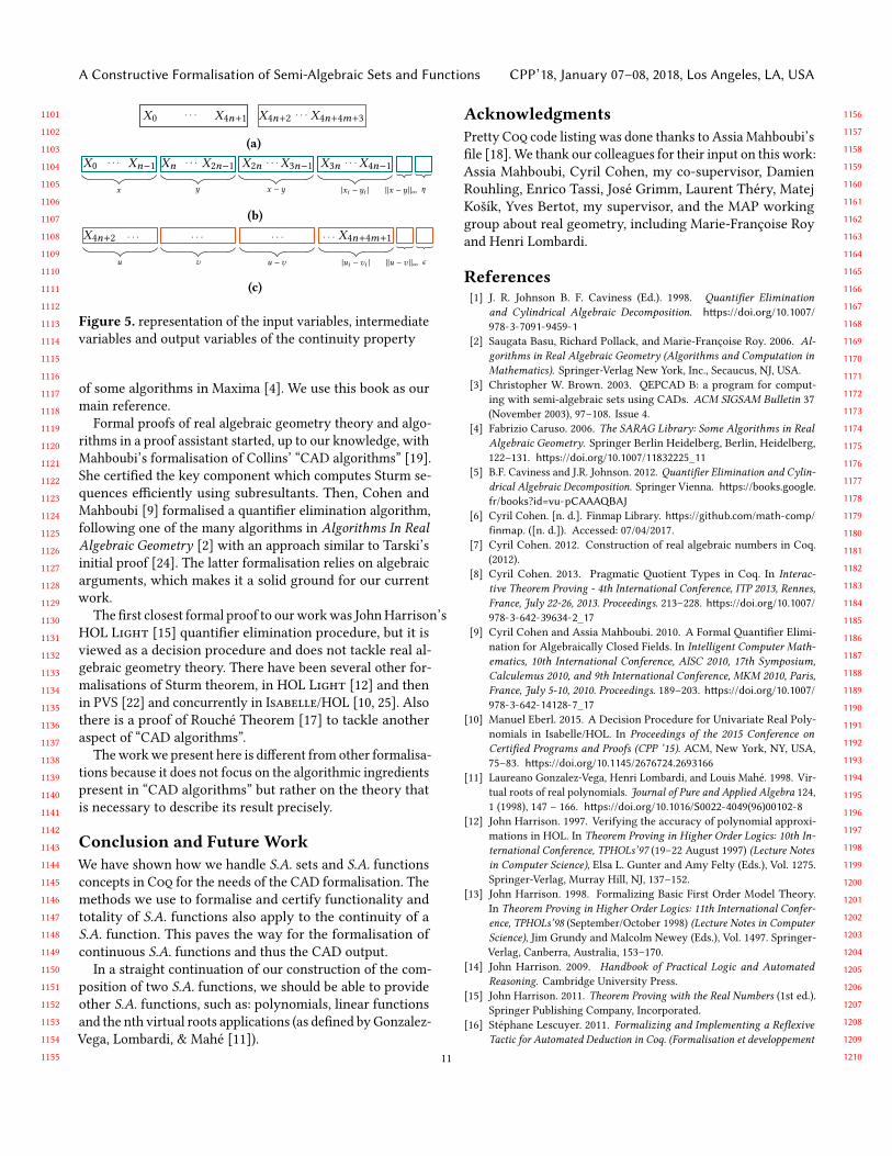
create a formula (8) representing the subtraction x − y. Thisformula has a third variables block to represent the output x−y and a subformula to express the ternary relation betweenx , y and x − y. Then, we create a formula (8) representingcoordinate-wise absolute value. This formula has a block torepresent z, a block to represent the vector ( |zi |)i , (0 ≤ i < n),and a subformula to express the binary relation betweenz and ( |zi |)i . We apply it to represent the vector |xi − yi |(0 ≤ i < n). Finally, we create a formula (8) representing thecoordinates maximum of a vector. This formula has a blockto represent z, a single variable to represent max0≤i<n ziand a subformula to represent the relation between z andmax0≤i<n zi . We apply it to represent ∥x − y∥∞.

Block Reasoning Extension In this paragraph, we extendblock reasoning with block subtraction (8), block absolutevalue (8) and block maximum (8).

These constructions are parameterised by the desired se-quences of variables

9

9919929939949959969979989991000100110021003100410051006100710081009101010111012101310141015101610171018101910201021102210231024102510261027102810291030103110321033103410351036103710381039104010411042104310441045


1046

1047

1048

1049

1050

1051

1052

1053

1054

1055

1056

1057

1058

1059

1060

1061

1062

1063

1064

1065

1066

1067

1068

1069

1070

1071

1072

1073

1074

1075

1076

1077

1078

1079

1080

1081

1082

1083

1084

1085

1086

1087

1088

1089

1090

1091

1092

1093

1094

1095

1096

1097

1098

1099

1100

Definition sub_vec (v1 v2 v3 : seq nat) : formula F :=if ((size v1 == size v2) && (size v1 == size v3))

then \big[And/True]_(i < size v1) ( 'X_(nth O v1 i) =='X_(nth O v2 i) + 'X_(nth O v3 i))%oT

else False.

Definition abs_vec (v1 v2 : seq nat) : formula F :=if size v1 == size v2

then (\big[And/True]_(i < size v1) (abs (nth O v1 i)) (nth O v2 i))%oT

else False.

Definition max_vec (v : seq nat) (n : nat) : formula F :=((\big[Or/False]_(i < size v) ('X_n == 'X_(nth O v i))) /\(\big[And/True]_(i < size v) ('X_(nth O v i) <=% 'X_n)))%oT.We also prove the following correctness properties for sub_vecand abs_vec, in Coq:

Lemma sub_vecP (e : seq F) (v1 v2 v3 : seq nat) :rcf_sat e (sub_vec v1 v2 v3) = ((size v1 == size v2) && (size v1

== size v3)) &&[forall i,(e_(nth O v3 (i : 'I_(size v1))) == e_(nth O v1 i) − e_(nth O v2 i))].

Lemma abs_vecP (e : seq F) (v1 v2 : seq nat) :rcf_sat e (abs_vec v1 v2) = (size v1 == size v2)

&& [forall i, e_(nth O v2 (i : 'I_(size v1))) == |e_(nth O v1 i)|].

We now come back to the reification of κ. ♦

To reify κ, each S.A. function application occurring inκ (subtraction, absolute value, maximum and f) requiresvariables 'X_i to represent both its inputs and its ouput. Letdenote the output dimension of f by p, in other words f hastype Rn → Rp .We need n variables to represent x , n variables to repre-

sent y, n variables to represent x −y, n variables to representthe row |xi − yi | (0 ≤ i < n), one variable to represent∥x − y∥∞ = max

0≤i<n|xi − yi | and one variable to represent η.

Similarly, we needm variables to represent u,m variablesto represent v ,m variables to represent u − v ,m variablesto represent the row |ui − vi | (0 ≤ i < n), one variable torepresent ∥u − v ∥∞ = max

0≤i<n|ui − vi | and one variable to

represent ϵ .We choose to represent x by the consecutive variables 'X_0. . . , 'X_(n - 1), y by the consecutive variables 'X_n, . . . ,'X_(2*n - 1), x −y by the consecutive variables 'X_(2*n),. . . , 'X_(3*n - 1), |xi − yi | (0 ≤ i < n) by the consecu-tive variables 'X_(3*n), . . . , 'X_(4*n - 1), ∥x −y∥∞ by thevariable 'X_(4*n) and η by the variable 'X_(4*n + 1) (seeFig. 5b).

We use a similar variable representation for the subformula∥u−v ∥∞ ≤ ϵ , starting at index 4*n + 2. We choose to repre-sent u by the consecutive variables 'X_0 . . . , 'X_(n - 1), vby the consecutive variables 'X_n, . . . , 'X_(2*n - 1), u −vby the consecutive variables 'X_(2*n), . . . , 'X_(3*n - 1),|ui −vi | (0 ≤ i < n) by the consecutive variables 'X_(3*n),. . . , 'X_(4*n - 1), ∥u −v ∥∞ by the variable 'X_(4*n) andϵ by 'X_(4*n + 1) (see Fig. 5c).

Indeed, the reification of ∥u − v ∥∞ ≤ ϵ is obtained byreifying ∥x − y∥∞ ≤ η form instead of n and by renamingvariables by shifting indices by 4n + 2 positions.

By exploiting block reasoning on our variable represen-tation, ∥x − y∥∞ ≤ η reifies to the following Coq formulaapplied to n:

Definition bloc (i : nat) : formula F :=(sub_vec (iota 0 i) (iota i i) (iota (2∗i) i))/\ (abs_vec (iota (2∗i) i) (iota (3∗i) i))/\ (max_vec (iota (3∗i) i) (4∗i))/\ ('X_(4∗i) <=% 'X_((4∗i).+1)).

To reify ∥u −v ∥∞ ≤ ϵ , we thus rename variables 'X_0 . . . ,'X_(4*m + 1) to 'X_(4*n + 2) . . . , 'X_(4*n + 4*m + 3)in bloc m, with block substitution: ∥u −v ∥∞ ≤ ϵ reifies to:

subst_formula (iota (4∗n + 2) (4∗m + 1)) (bloc m)

thus, κ reifies to:

(bloc n) ==> (subst_formula (iota (4∗n + 2) (4∗m + 1)) (bloc m))

whichwe denote by beta. We now have to restrictκ to valuesx , y, u and v such that f (x ) = u and f (y) = v . We alreadyknow how to reify the latter equations by applying blocksubstitutions on f ; we reify the quantifier-free part of thecontinuity property in Coq with:

beta /\ (subst_formula ((iota 0 n) ++ (iota (4∗n + 2) m)) f)/\ (subst_formula ((iota n n) ++ (iota (4∗n + m + 2) m)) f).

which we denote by gamma.We now achieve the full reification of the continuity prop-

erty by adding all the quantifications with:

Definition is_continuous_form (f : {formula_(n + m) F}) :=nquantify 0 n Forall

('forall 'X_(4∗n + 4∗m + 3),('exists 'X_(4∗n + 1), (nquantify n (2∗n) Forall(nquantify (2∗n) (2∗n + 1) Forall(nquantify (4∗n + 2) (4∗m + 1) Forall gamma))))).

9 Related WorkThe main related work is the book Algorithms In Real Al-gebraic Geometry [2], which describes various algorithmsincluding “CAD algorithms”. While this book contains “pa-per” algorithms and proofs, it comes with implementations

10

1101110211031104110511061107110811091110111111121113111411151116111711181119112011211122112311241125112611271128112911301131113211331134113511361137113811391140114111421143114411451146114711481149115011511152115311541155


1156

1157

1158

1159

1160

1161

1162

1163

1164

1165

1166

1167

1168

1169

1170

1171

1172

1173

1174

1175

1176

1177

1178

1179

1180

1181

1182

1183

1184

1185

1186

1187

1188

1189

1190

1191

1192

1193

1194

1195

1196

1197

1198

1199

1200

1201

1202

1203

1204

1205

1206

1207

1208

1209

1210

· · · · · ·X0 X4n+1 X4n+2 X4n+4m+3

(a)X0 Xn−1· · ·

x

Xn X2n−1· · ·

y

X2n X3n−1· · ·

x − y

X3n X4n−1· · ·

|xi − yi | ∥x − y∥∞ η

(b)X4n+2 · · ·

u

· · ·

v

· · ·

u −v

X4n+4m+1· · ·

|ui −vi | ∥u −v ∥∞ ϵ

(c)

Figure 5. representation of the input variables, intermediatevariables and output variables of the continuity property

of some algorithms in Maxima [4]. We use this book as ourmain reference.

Formal proofs of real algebraic geometry theory and algo-rithms in a proof assistant started, up to our knowledge, withMahboubi’s formalisation of Collins’ “CAD algorithms” [19].She certified the key component which computes Sturm se-quences efficiently using subresultants. Then, Cohen andMahboubi [9] formalised a quantifier elimination algorithm,following one of the many algorithms in Algorithms In RealAlgebraic Geometry [2] with an approach similar to Tarski’sinitial proof [24]. The latter formalisation relies on algebraicarguments, which makes it a solid ground for our currentwork.

The first closest formal proof to ourworkwas JohnHarrison’sHOL Light [15] quantifier elimination procedure, but it isviewed as a decision procedure and does not tackle real al-gebraic geometry theory. There have been several other for-malisations of Sturm theorem, in HOL Light [12] and thenin PVS [22] and concurrently in Isabelle/HOL [10, 25]. Alsothere is a proof of Rouché Theorem [17] to tackle anotheraspect of “CAD algorithms”.

Theworkwe present here is different from other formalisa-tions because it does not focus on the algorithmic ingredientspresent in “CAD algorithms” but rather on the theory thatis necessary to describe its result precisely.

Conclusion and Future WorkWe have shown how we handle S.A. sets and S.A. functionsconcepts in Coq for the needs of the CAD formalisation. Themethods we use to formalise and certify functionality andtotality of S.A. functions also apply to the continuity of aS.A. function. This paves the way for the formalisation ofcontinuous S.A. functions and thus the CAD output.

In a straight continuation of our construction of the com-position of two S.A. functions, we should be able to provideother S.A. functions, such as: polynomials, linear functionsand the nth virtual roots applications (as defined byGonzalez-Vega, Lombardi, & Mahé [11]).

AcknowledgmentsPrettyCoq code listing was done thanks to Assia Mahboubi’sfile [18].We thank our colleagues for their input on this work:Assia Mahboubi, Cyril Cohen, my co-supervisor, DamienRouhling, Enrico Tassi, José Grimm, Laurent Théry, MatejKošík, Yves Bertot, my supervisor, and the MAP workinggroup about real geometry, including Marie-Françoise Royand Henri Lombardi.

References[1] J. R. Johnson B. F. Caviness (Ed.). 1998. Quantifier Elimination

and Cylindrical Algebraic Decomposition. https://doi.org/10.1007/978-3-7091-9459-1

[2] Saugata Basu, Richard Pollack, and Marie-Françoise Roy. 2006. Al-gorithms in Real Algebraic Geometry (Algorithms and Computation inMathematics). Springer-Verlag New York, Inc., Secaucus, NJ, USA.

[3] Christopher W. Brown. 2003. QEPCAD B: a program for comput-ing with semi-algebraic sets using CADs. ACM SIGSAM Bulletin 37(November 2003), 97–108. Issue 4.

[4] Fabrizio Caruso. 2006. The SARAG Library: Some Algorithms in RealAlgebraic Geometry. Springer Berlin Heidelberg, Berlin, Heidelberg,122–131. https://doi.org/10.1007/11832225_11

[5] B.F. Caviness and J.R. Johnson. 2012. Quantifier Elimination and Cylin-drical Algebraic Decomposition. Springer Vienna. https://books.google.fr/books?id=vu-pCAAAQBAJ

[6] Cyril Cohen. [n. d.]. Finmap Library. https://github.com/math-comp/finmap. ([n. d.]). Accessed: 07/04/2017.

[7] Cyril Cohen. 2012. Construction of real algebraic numbers in Coq.(2012).

[8] Cyril Cohen. 2013. Pragmatic Quotient Types in Coq. In Interac-tive Theorem Proving - 4th International Conference, ITP 2013, Rennes,France, July 22-26, 2013. Proceedings. 213–228. https://doi.org/10.1007/978-3-642-39634-2_17

[9] Cyril Cohen and Assia Mahboubi. 2010. A Formal Quantifier Elimi-nation for Algebraically Closed Fields. In Intelligent Computer Math-ematics, 10th International Conference, AISC 2010, 17th Symposium,Calculemus 2010, and 9th International Conference, MKM 2010, Paris,France, July 5-10, 2010. Proceedings. 189–203. https://doi.org/10.1007/978-3-642-14128-7_17

[10] Manuel Eberl. 2015. A Decision Procedure for Univariate Real Poly-nomials in Isabelle/HOL. In Proceedings of the 2015 Conference onCertified Programs and Proofs (CPP ’15). ACM, New York, NY, USA,75–83. https://doi.org/10.1145/2676724.2693166

[11] Laureano Gonzalez-Vega, Henri Lombardi, and Louis Mahé. 1998. Vir-tual roots of real polynomials. Journal of Pure and Applied Algebra 124,1 (1998), 147 – 166. https://doi.org/10.1016/S0022-4049(96)00102-8

[12] John Harrison. 1997. Verifying the accuracy of polynomial approxi-mations in HOL. In Theorem Proving in Higher Order Logics: 10th In-ternational Conference, TPHOLs’97 (19–22 August 1997) (Lecture Notesin Computer Science), Elsa L. Gunter and Amy Felty (Eds.), Vol. 1275.Springer-Verlag, Murray Hill, NJ, 137–152.

[13] John Harrison. 1998. Formalizing Basic First Order Model Theory.In Theorem Proving in Higher Order Logics: 11th International Confer-ence, TPHOLs’98 (September/October 1998) (Lecture Notes in ComputerScience), Jim Grundy and Malcolm Newey (Eds.), Vol. 1497. Springer-Verlag, Canberra, Australia, 153–170.

[14] John Harrison. 2009. Handbook of Practical Logic and AutomatedReasoning. Cambridge University Press.

[15] John Harrison. 2011. Theorem Proving with the Real Numbers (1st ed.).Springer Publishing Company, Incorporated.

[16] Stéphane Lescuyer. 2011. Formalizing and Implementing a ReflexiveTactic for Automated Deduction in Coq. (Formalisation et developpement

11

1211121212131214121512161217121812191220122112221223122412251226122712281229123012311232123312341235123612371238123912401241124212431244124512461247124812491250125112521253125412551256125712581259126012611262126312641265


1266

1267

1268

1269

1270

1271

1272

1273

1274

1275

1276

1277

1278

1279

1280

1281

1282

1283

1284

1285

1286

1287

1288

1289

1290

1291

1292

1293

1294

1295

1296

1297

1298

1299

1300

1301

1302

1303

1304

1305

1306

1307

1308

1309

1310

1311

1312

1313

1314

1315

1316

1317

1318

1319

1320

d’une tactique reflexive pour la demonstration automatique en coq).Ph.D. Dissertation. University of Paris-Sud, Orsay, France. https://tel.archives-ouvertes.fr/tel-00713668

[17] Wenda Li and Lawrence C. Paulson. 2016. A Formal Proof of Cauchy’sResidue Theorem. Springer International Publishing, Cham, 235–251.https://doi.org/10.1007/978-3-319-43144-4_15

[18] Assia Mahboubi. [n. d.]. lstcoq.sty file which defines a Coq - SSReflectstyle for listings in Latex. https://hal.inria.fr/file/index/docid/611757/filename/lstcoq.sty. ([n. d.]). Accessed: 08/02/2017.

[19] Assia Mahboubi. 2006. Contributions à la certification des calculsdans R : théorie, preuves, programmation. (Contributions to the certifi-cation of computations in R : theory, proofs, implementation). Ph.D.Dissertation. University of Nice Sophia Antipolis, France. https://tel.archives-ouvertes.fr/tel-00117409

[20] Assia Mahboubi. 2007. Implementing the Cylindrical Algebraic Decom-positionWithin the Coq System. Mathematical. Structures in Comp. Sci.17, 1 (Feb. 2007), 99–127. https://doi.org/10.1017/S096012950600586X

[21] Assia Mahboubi and Enrico Tassi. [n. d.]. Mathematical Components.https://math-comp.github.io/mcb/. ([n. d.]). Accessed: 06/04/2017.

[22] Anthony Narkawicz, César Muñoz, and Aaron Dutle. 2015. Formally-Verified Decision Procedures for Univariate Polynomial ComputationBased on Sturm’s and Tarski’s Theorems. Journal of Automated Reason-ing 54, 4 (2015), 285–326. https://doi.org/10.1007/s10817-015-9320-x

[23] Christine Paulin-Mohring. 2011. Introduction to the Coq Proof-Assistant for Practical Software Verification. In Tools for PracticalSoftware Verification, LASER, International Summer School 2011, ElbaIsland, Italy, Revised Tutorial Lectures. 45–95. https://doi.org/10.1007/978-3-642-35746-6_3

[24] Alfred Tarski. 1951. A decision method for elementary algebra andgeometry. Bull. Amer. Math. Soc. 59 (1951).

[25] Lawrence C. Paulson Wenda Li, Grant Olney Passmore. 2015. A Com-plete Decision Procedure for Univariate Polynomial Problems in Is-abelle/HOL. (2015).

[26] Wikipedia. [n. d.]. CAD. https://en.wikipedia.org/wiki/Cylindrical_algebraic_decomposition. ([n. d.]). Accessed: 11/04/2017.

12

A Constructive Formalisation of Semi-algebraic Sets and ...

Documents

Transcript of A Constructive Formalisation of Semi-algebraic Sets and ...