A constitutive equation for thixotropic suspensions with yield stress by coarse-graining apopulation balance model

Paul M. Mwasame, Antony N. Beris, R. B. Diemer, Norman J. Wagner1

Center for Molecular and Engineering Thermodynamics, Department of Chemical and Biomolecular Engineering, University of Delaware, Newark, DE 19716

Abstract

A population balance model appropriate for the shear flow of thixotropic colloidal suspensions with yield stress is derived and

tested against experimental data on a model system available in the literature. Modifications are made to account for dynamic

arrest at the onset of the yield stress, in addition to enforcing a minimum particle size below which breakage is not feasible. The

resulting constitutive model also incorporates a structural based relaxation time, unlike existing phenomenological models that use

the inverse of the material shear rate as the relaxation time. The model provides a reasonable representation of experimental data

for a model thixotropic suspension in the literature, capturing the important thixotropic timescales. When compared to prevalent

structure kinetics models, the coarse grained population balance equation is shown to be distinct, emphasizing the novelty of

utilizing population balances as a basis for thixotropic suspension modeling.

1. Introduction

Ideal thixotropy is defined as the continuous decrease of

viscosity with time when flow is applied to a sample that has

been previously at rest, and the subsequent recovery of viscosity

when flow is discontinued [1]. In colloidal suspensions, the mi-

crostructure evolution thought to underly thixotropic behavior

includes the formation of aggregates and even network struc-

tures that are associated with a yield stress [2]. These structures

can undergo breakage under flow revealing the complex inter-

play between rheology and microstructure. Thixotropic sus-

pensions are also inherently multiscale in nature, with multiple

length scales leading to multiple time scales that also depend

on the flow conditions. This explains much of the complex

non-Newtonian rheological behavior, including hysteresis and

viscoelasticity, observed in these systems [3, 4]. More detailed

1Corresponding Author: wagnernj@udel.edu

reviews on this subject are offered by Mewis [5], Barnes [6] and

Mewis and Wagner [7].

Thixotropic media are frequently encountered in large-scale

industrial processes including oil pipeline-transport, red-mud in

minerals processing [8] and waste processing at superfund sites

[9]. In addition, thixotropic agents are prominent in consumer

applications, such as beauty creams [10], and have even been

proposed for gelled hydrocarbon fuel applications [11]. Print-

ing inks [12, 13] and even blood can be considered thixotropic

[14]. The breadth and growing importance of these applica-

tions coupled with environmental concerns justifies the consid-

erable effort put into developing predictive models for such sys-

tems. At the heart of these modeling efforts is the relationship

between microstructure and rheology. Consequently, models

incorporating microstructural variables are required to under-

stand, interpret and predict rheological behavior of such sys-

tems.

Preprint submitted to AIChE Journal August 2, 2016

The earliest formal use of a structural variable to model the

structural dynamics in a thixotropic suspension can be traced

back to the work of Goodeve [15]. At the heart of this ap-

proach is the concept that structural changes govern the rhe-

ology of thixotropic suspensions, and these can be accounted

for by tracking the creation and destruction of ’bonds’ in the

system. This ’structure kinetic’ approach has been applied with

some success in developing rheological constitutive equations

for thixotropic suspensions [14, 16], but with limitations. The

most glaring deficiency is the difficulty in unambiguously re-

lating the order parameter describing creation and breakage of

bonds to experimental measurements of the microstructure. Fur-

thermore, the structure kinetic equations are phenomenological

as they contain parameters that cannot be directly interpreted in

terms of the properties of the suspension of particles. Therefore,

it is desirable to develop new theoretical approaches that relate

structural changes in a thixotropic suspensions to fundamental

processes and properties at the particle level.

This work develops a macroscopic rheological model for

thixotropic suspensions based on population balances [17, 18].

Our effort is aided by the extensive literature available on char-

acteristic rate processes [19, 20, 21] and fractal scaling theo-

ries applicable to aggregating colloidal dispersions. Previous

efforts have related the rheology of colloidal dispersions to mi-

crostructural changes through the use of population balances.

von Smoluchowski [22] may have been the first one to connect

colloidal aggregation to suspension viscosity. Barthelemes et

al. [23] applied a coupling between a sectional population bal-

ance model and a rheological law to describe the viscosity of

a flowing suspension. Mohtaschemi et al. [24] also applied

a similar approach to describe the rheology of an aggregating

colloidal suspension. All these studies point to the important

role microstructure plays in determining the rheology of aggre-

gating soft colloidal suspensions and the promise of population

balances.

Despite the success of population balances in modeling the

microstructure and rheology, these studies were limited to purely

viscous suspensions and are not applicable to thixotropic sus-

pensions with a yield stress. In this work we address the two

main challenges in developing such a theory: 1) How to ac-

count for the dynamical arrest characterized as a yield stress;

and 2) How to coarse grain the theory to yield an efficient model

that retains sufficient connection between particle-level proper-

ties and emergent rheological behavior and free from unneces-

sary phenomenology. By applying appropriate model assump-

tions, different from the preceding works, we develop a coarse-

grained, single variable, evolution equation that accounts for

structural changes in thixotropic suspensions with a yield stress.

A constitutive equation is required to calculate the suspen-

sion rheology (shear stress) from the structural predictions aris-

ing from the coarse grained population balance equation. The

formulation of a constitutive relationship for thixotropic sus-

pensions remains an open question [7]. In this work a simple,

phenomenological constitutive relationship that sums a structure-

dependent viscous contribution and a structure-dependent elas-

tic contribution is assumed. More generally, the coarse-grained

population balance equation developed here can, in principle,

be used in any existing constitutive model for thixotropy that in-

corporates an appropriate structural variable. Therefore, the fo-

cus of the present work is the development of a coarse-grained

population balance model appropriate for thixotropic suspen-

sions with yield stress. For the purposes of illustrating and vali-

dating the model, we use the recently published data set of Arm-

strong et al. [25] that expands upon the experimental data on a

model system first proposed by Dullaert and Mewis [26]. This

data set, available online, is for a thixotropic silica suspension

and includes a broad range of rheological experiments includ-

ing steady-state, transient step-up and step-down, flow reversal

2

and oscillatory shear experiments.

In the following, we begin with a brief description of the

development of a population-based model for thixotropic sus-

pensions experiencing shear flow. The coarse-graining of the

population balance equation is then carried out through the mo-

ment method. Next, we address further modifications neces-

sary to describe concentrated thixotropic suspensions that dis-

play a yield stress. A phenomenological constitutive relation-

ship is then proposed to link the microstructural calculations

arising from the population balance to the macroscopic stress

that is measured in rheological experiments. The model param-

eterization is then described and subsequent validation is per-

fomed using a rheology dataset available in the literature [25].

The model predictions are discussed and tested against oscilla-

tory shear and flow reversal experiments. Finally, the coarse-

grained population balance equation is compared against the

phenomenological structure kinetic one followed by a discus-

sion of the main conclusions.

2. Theory

2.1. The population balance model

In suspensions, aggregation of colloidal particles gives rise

to fractal-like aggregate structures that exhibit self-similarity

over multiple length scales [27]. These emerging additional

scales make thixotropic suspensions challenging to model. How-

ever, by applying existing knowledge and appropriate theories

describing aggregation and breakage at the particle level, we

can build an approximate but detailed microscopic description

of the evolution of suspension microstructure in shear flows.

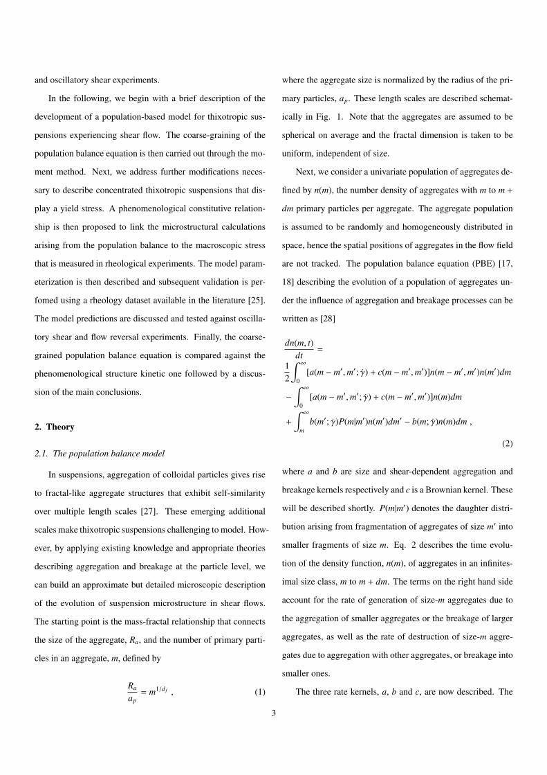
The starting point is the mass-fractal relationship that connects

the size of the aggregate, Ra, and the number of primary parti-

cles in an aggregate, m, defined by

Ra

ap= m1/d f , (1)

where the aggregate size is normalized by the radius of the pri-

mary particles, ap. These length scales are described schemat-

ically in Fig. 1. Note that the aggregates are assumed to be

spherical on average and the fractal dimension is taken to be

uniform, independent of size.

Next, we consider a univariate population of aggregates de-

fined by n(m), the number density of aggregates with m to m +

dm primary particles per aggregate. The aggregate population

is assumed to be randomly and homogeneously distributed in

space, hence the spatial positions of aggregates in the flow field

are not tracked. The population balance equation (PBE) [17,

18] describing the evolution of a population of aggregates un-

der the influence of aggregation and breakage processes can be

written as [28]

dn(m, t)dt

=

12

∫ ∞

0[a(m − m′,m′; γ) + c(m − m′,m′)]n(m − m′,m′)n(m′)dm

−

∫ ∞

0[a(m − m′,m′; γ) + c(m − m′,m′)]n(m)dm

+

∫ ∞

mb(m′; γ)P(m|m′)n(m′)dm′ − b(m; γ)n(m)dm ,

(2)

where a and b are size and shear-dependent aggregation and

breakage kernels respectively and c is a Brownian kernel. These

will be described shortly. P(m|m′) denotes the daughter distri-

bution arising from fragmentation of aggregates of size m′ into

smaller fragments of size m. Eq. 2 describes the time evolu-

tion of the density function, n(m), of aggregates in an infinites-

imal size class, m to m + dm. The terms on the right hand side

account for the rate of generation of size-m aggregates due to

the aggregation of smaller aggregates or the breakage of larger

aggregates, as well as the rate of destruction of size-m aggre-

gates due to aggregation with other aggregates, or breakage into

smaller ones.

The three rate kernels, a, b and c, are now described. The

3

Figure 1: An illustration of the multiple length scales present in the aggregate network of a thixotropic suspension showing the primary particles of diameter 2ap(A), primary clusters of diameter 2apc (B), viscometric volume of the aggregates characterized by diameter 2Rh (C) and an effective volume of the aggregatescharacterized by diameter 2Ra (D).

first is the rate of shear driven aggregation between aggregagtes

of mass m and m′, which was derived by von Smoluchowski

[19] and is given by

a(m,m′; γ) =43αa3

p|γ|(m1/d f + m′1/d f

)3, (3)

where γ is the shear rate and α is the collision efficiency. Next,

the rate of Brownian aggregation, also derived by von Smolu-

chowski [19, 20], is given by

c(m,m′) =

(2kBT3µsW

) (m1/d f + m′1/d f

) (m−1/d f + m′−1/d f

), (4)

where kB is Boltzmann’s constant, T is the temperature in Kelvin,

µs is the medium or solvent viscosity, W is the Fuch’s stability

ratio [29] and d f is the fractal dimension. A detailed review of

flocculation models is presented by Thomas et al. [30].

Two main approaches have been proposed in the literature

to the describe the breakage rate kernel, b: exponential and

power law kernels. The latter is used in this work. Particle

breakage occurs when a stress acting on an aggregate exceeds

its cohesive strength. One may consider two types of stresses

that can cause breakage, (i) stresses induced by collisions and

(ii) stresses caused by velocity gradients in the fluid [31]. In

this work, we adopt a power law breakage kernel that casts the

functional dependence of breakage frequency as a product of

the size of aggregates and the shear rate that provides the driv-

ing force for breakup. Following Spicer and Pratsinis [21], the

breakage rate of aggregates in a shear field is given by

b(m; γ) = bo|γ|2m1/d f , (5)

where bo is a pre-factor. Given Eq. 1, the breakage rate is

assumed to depend linearly on the aggregate size.

4

2.2. Coarse graining the population balance equation

In practice, solving Eq. 2 using the auxilliary Eqs. 3-5

is not a simple task because it is an integro-differential equa-

tion and the rate processes depend on the mass m of the aggre-

gates. However, we do not necessarily require all the informa-

tion present in the aggregate size distribution, n(m). Therefore,

the method of moments is used to extract only the relevant in-

formation needed from the aggregate size distribution [32, 33].

Still, the moment equations may constitute an open set of cou-

pled equations owing to the non-linear aggregation and break-

age rate processes in Eqs. 3-5. Therefore, additional coarse

graining involving assumptions about the underlying aggregate

size distribution must be performed to obtain an approximate

but closed set of moment equations that are more useful for en-

gineering applications [34].

The kth moment of the aggregate size distribution, Mk , is

defined by

Mk =

∫ ∞

0mkn(m)dm . (6)

However, it is preferable to work in terms of the scaled aggre-

gate size distribution, n(m), given by

n(m)dm =n(m)dm

N0, (7)

where the normalization constant, No, is the total number of

primary particles per unit volume in the suspension. The corre-

sponding scaled moments, µk, are then defined as

µk =Mk

N0=

∫ ∞

0mkn(m)dm , (8)

Physically, the zeroth scaled moment, µ0, represents the re-

ciprocal of the average aggregation number while the first mo-

ment, µ1, is the total mass of primary particles, which is a con-

served quantity in a closed system. It is readily observed that µ0

is a bounded quantity, taking on values between 0 and 1, while

µ1 = 1 reflecting mass conservation. The set of scaled moment

equations, equivalent to the PBE in Eq. 2, is given by

dµk(t)dt

=

12

No

∫ ∞

0n(λ)

∫ ∞

0[a(λ, ε) + c(λ, ε)]n(ε)dεdλ

− No

∫ ∞

0mkn(m)

∫ ∞

0[a(λ, ε) + c(λ, ε)]n(ε)dλdm

+

∫ ∞

0λkb(λ)n(λ)dλ (θk − 1) .

(9)

The simplification in the last term of this equation is possible by

assuming that the daughter distribution, P(m|m′), depends only

on the relative ratio ξ = m/m′ [33]. Physically, self-similar

breakage representes a scenario in which all aggregates possess

the same daughter distribution regardless of the parent aggre-

gate size. Such a self-similar daughter distribution is defined

by P(ξ) with moments, θk, given by

θk =

∫ 1

0ξkP (ξ) dξ . (10)

As will be shown shortly in the coarse-graining, only the zeroth

moment of the daughter distribution, θ0, physically representing

the number of fragments formed during a breakage event, is

required here. Therefore, the particular form of P(ξ) does not

need to be specified.

The rate kernels in Eqs. 3-5 together with Eq. 9, yield the

following equations for the first three moments

dµ0

dt= −

kTφp

2µsWπa3p

(µ20 + µ−1/d f µ1/d f

)− α|γ|

(φp

π

) (µ0µ3/d f + 3µ2/d f µ1/d f

)+ bo|γ|

2µ1/d f (θ0 − 1) ,

(11)

dµ1

dt= 0 , (12)

5

dµ2

dt= −

kTφp

2µsWπa3p

(2µ21 + 2µ1+1/d f µ1−1/d f

)− α|γ|

(φp

π

) (2µ1µ1+3/d f + 6µ1+2/d f µ1+1/d f

)+ bo|γ|

2µ2+1/d f (θ2 − 1) .

(13)

The volume fraction of the primary particles, φp, enters the

above equations through the following relationship

φp =43πa3

pN0 . (14)

In the moment equations above, Eqs. 11 - 13, the stability ratio

(W), collision efficiency (α), breakage pre-factor (bo), fractal

dimension (d f ) and moments of the daughter distribution (θk)

are microscopic parameters. In principle, all of these parame-

ters may be determined from independent experiments or the-

ory as they represent physical properties of the particles and

aggregates.

The resulting set of moment equations is not closed and also

involves fractional moments. A closure rule is required to facil-

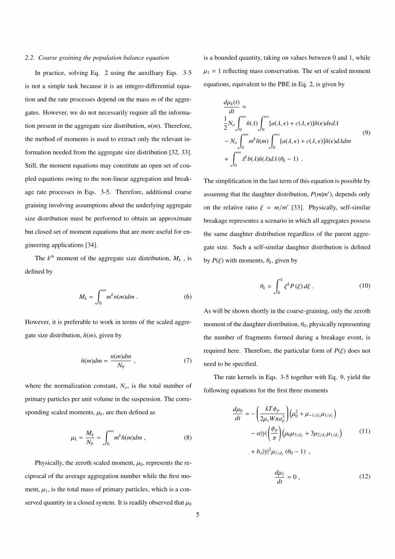
itate numerical solutions. The closure rule adopted in this work

is that the population of aggregates is monodisperse at each step

in its trajectory [35, 33]. This simple assumption is depicted in

Fig. 2, and is represented mathematically as

n(m) = µ0δ (m − mn) . (15)

The additional variable mn appearing in the delta function above

represents the average number of primary particles per aggre-

gate, and is given by

mn = µ1/µ0 = 1/µ0 . (16)

The moments of the distribution described in Eq. 15 are

Figure 2: A physical representation of the monodisperse closure rule. The realsystem (left) is represented by an idealized system (right) in which the mass isdistributed equally over all aggregates in the system.

given by

µk =

∫ ∞

0mkµ0 (m − mn) dm = µ0mk

n = µ1−k0 . (17)

This closure rule allows for the simplification of the infinite set

of moment equations, Eq. 9, to a single dynamic equation for

the zeroth moment

dµ0

dt= − 2

kTφp

2µsWπa3p

µ20 − 4α|γ|

(φp

π

)µ

2−3/d f

0

+ bo|γ|2µ

1−1/d f

0 (θ0 − 1) ,

(18)

and an algebraic equation for all higher order moments

µk = µ1−k0 µk

1 . (19)

Eq. 18 describes the evolution of the reciprocal of the agge-

gation number µ0. The first term on the right hand side of Eq.

18 represents the effect of Brownian aggregation while the sec-

ond and third represent shear aggregation and shear breakage

respectively. The important outcome here is that the integro-

differential population balance model can now be represented

by a single ordinary differential equation for the zeroth moment.

Furthermore, this closure rule eliminates the need to specify a

particular daughter distribution, only requiring information on

6

the number of fragments produced during a breakage event θ0

The framework applied so far to describe aggregation and

breakage kinetics of colloidal aggregates was originally derived

for dilute suspensions [19] and has been successfully applied

by multiple authors [21, 23, 35, 36] using the moment method.

However, the structure dynamics in a concentrated thixotropic

suspension strongly deviate from this idealized picture because

fractal aggregates can fill space, leading to dynamic arrest and

a yield stress. Therefore, the limitations of the underlying ex-

pressions used in this section now need to be examined and

appropriate modifications made to extend their applicability to

typical suspensions encountered in practice.

2.3. Modifications necessary for thixotropic suspensions with

yield stress

In this section we discuss some necessary improvements,

albeit phenomenological and by no means unique, to ensure

the evolution equation for the zeroth moment closely describes

experimental observations.

2.3.1. Incorporating dynamic arrest

Suspensions of practical relevance are typically more con-

centrated [16, 37] than those studied by previous authors [21,

23, 35, 36]. This means we have to include additional physics

into the rate processes describing aggregation and breakage pro-

cesses. Rheological experiments on thixotropic suspension pro-

vide some guidance on how to do this. In particular, an impor-

tant observation by Dullaert and Mewis [37] is that of a yield

stress at finite shear viscosity. This means that the increase in

hydrodynamic viscosity due to presence of aggregates alone is

not sufficient to explain the dynamic arrest when a space filling

network forms. Rather, a network elasticity due to percolation

of the aggregates is what gives rise to the yield stress.

As aggregation proceeds, hydrodynamic interactions inten-

sify noticeably [38]. To account for this, the aggregation rate

should be calculated by considering that each aggregate exists

in an effective medium of other aggregates. This is accom-

plished by replacing the medium viscosity, µs, by the effective

suspension viscosity, µsηhr , in the Brownian aggregation kernel

in Eq 4 resulting in

c(λ, ε) =

(2kT

3µsηhr W

) (λ1/d f + ε1/d f

) (λ−1/d f + ε−1/d f

), (20)

where ηhr is the relative viscosity of the suspension. Although

many choices exist for describing the suspension viscosity [39,

40], the robust and simple Marron and Pierce [41] equation is

used to define the relative hydrodynamic viscosity as

ηhr =

(1 −

φh

φmax

)−2

. (21)

In this expression, φh is the viscometric volume fraction of the

porous aggregates while φmax is the maximum packing frac-

tion of the aggregates. Considering that a finite viscous contri-

bution to the viscosity is observed when the space filling net-

work forms [25], the hydrodynamic radius of the aggregate Rh

is smaller than the aggregate size Ra, i.e. the aggregates are

porous to the fluid. If we define the aggregate volume fraction

as

φa = φpµ1−3/d f

0 , (22)

the viscometric volume fraction that enters the viscosity calcu-

lation in Eq. 21 may be approximated by

φh =

(Rh

Ra

)3

φa , (23)

where Rh/Ra reflects the permeability of the fractal aggregates

and is assumed to be constant. This completes the first modifi-

cation to the Brownian aggregation rate kernel.

The porous nature of fractal aggregates means that the sus-

7

pension’s hydrodynamic viscosity does not diverge so as to ar-

rest perikinetic aggregation. Furthermore, at low shear rates,

the shear aggregation term (∼ γ) dominates the shear break-

age term (∼ γ2), leading to a run-away increase in aggregate

size. It is therefore possible for aggregates to grow to very large

sizes, allowing the configurational aggregate volume fraction,

φa, to exceed φmax. Such predictions are unphysical. To rem-

edy this, the emerging yield stress is identified as an indepen-

dent constraint on the trajectory of growing aggregates that sets

the maximum aggregate size. Mohtaschemi et al. [24] asso-

ciated dynamic arrest of perikinetic aggregation with trapping

of aggregates at high viscosities. They introduce a hyperbolic

cutoff function that arrests brownian aggregation once the sus-

pension viscosity exceeds a critical value ηc. In addition, their

viscosity calculation assumes the aggregates are impermeable.

Although, their approach is not directly applicable to dynamic

arrest in thixotropic suspensions of porous fractal aggregates

that exhibit a finite hyrodynamic viscosity and a yield stress

[37], we can adapt the concept to our model.

Dynamic arrest in the presence of porous fractal aggregates

is attributed to the increase in contact probability due to growth

of aggregates, which stops further growth once a space filling

network forms as φa approaches φmax. Thus the yielding behav-

ior arises from elastic stresses. This aggregate jamming effect is

modeled as an onset phenomenon by a hyperbolic cutoff func-

tion

β ≡ β(φa(µ0)) = tanh(χφmax − φa

φmax − φpc

), (24)

where β, 0 < β < 1, is an effective factor weighting the aggrega-

tion kernels a and c. The constant χ is assigned a value of 2.65,

chosen such that β approaches a value of 0.99 when all aggre-

gates are broken down to their minimum allowable size charac-

terized by a corresponding volume fraction φpc. The evaluation

of φpc is discussed later in this section. The order parameter(φmax−φaφmax−φpc

)describes the proximity to the yield stress, while β is

applied as a pre-multiplier to the shear and Brownian aggrega-

tion kernels. This completes the modification of the aggregation

processes.

2.3.2. Enforcing minimum breakage size

Depending on the pre-shear/pre-processing protocol, the ini-

tial rest state of the suspension may consist of permanent ag-

gregates of the constituent primary particles, referred to here

as primary clusters, which in turn can combine to form larger

aggregates depicted in Fig. 1. Primary clusters have been con-

firmed using small angle X-ray and neutron scattering [42, 43].

Rheologically, primary clusters are associated with a high shear

rate viscosity that significantly exceeds the expected theoretical

value based on the actual solids loading of the primary particles

φp. Therefore, a lower size bound must be enforced to ensure

that the aggregates never break below their smallest, allowable

size based on the suspension preparation protocol. Thus, at high

shear rates, the breakage rate should tend to zero as the aggre-

gates are broken down into their constituent primary clusters.

This requirement is enforced by modifying the breakage

rate in Eq. 5 to

b(m) = boγ2(m1/d f − m1/d f pc

p

), (25)

where mp is the number of primary particles in the primary clus-

ter. A value of mp = 1, implies the aggregates can be broken

down to the constituent primary particles of size a. The size

of the primary clusters may be estimated as apc = apm1/d f pcp ,

characterized by a second fractal dimension d f pc. Finally, φpc,

is associated with the cluster volume fraction, and calculated as

φpc = φpm(3/d f pc−1)p . The fractal dimension of the primary clus-

ter (d f pc) is equal to the aggregate fractal dimension (d f ). This

assumption can be relaxed if additional information about the

8

primary clusters is available.

2.3.3. Modified moment equation

To arrive at the modified set of moment equations we need

to pre-multiply Eqs. 3 and 20 for the aggregation kernels by Eq.

24 and use the new expression for the breakage kernel provided

by Eq. 25. These expressions are substituted into Eq. 9. By

applying the monodisperse closure rule as described in Section

2.2, the evolution equation for the zeroth moment is given by

dµ0

dt= − 2β

kTφp

2µsηhr Wπa3

p

µ20 − 4βα

(φp

π

)|γ|µ

2−3/d f

0

+ bo|γ|2(µ

1−1/d f

0 − m1/d f pcp µ0

)(θ0 − 1) ,

(26)

with all other moments provided by Eq. 19. Eq. 26 represents

the evolution of microstructure in a thixotropic suspension with

a yield stress while also allowing for the existence of primary

clusters for mp , 1. Next, a constitutive equation for the shear

stress, incorporating µ0 as the microstructural variable, is spec-

ified to complete the model development.

2.4. Constitutive model for the shear stress

The rigorous development of an appropriate constitutive re-

lationship for the stress tensor based on microscopic insights

remains a challenge and is not addressed in this work. Rather,

a semi-empirical expression for the shear stress is developed

to interpret rheological data. More specifically, the constitu-

tive relationship assumes that stress is given by a superposition

of elastic and viscous, i.e. purely hydrodynamic, contributions

[6, 16].

σ = σelastic + σviscous . (27)

The structural variable, µ0, is linked to the various contri-

butions to the macroscopic stress, σ, as follows. The viscosity

of the aggregates is computed by assuming knowledge of the

viscometric volume of the aggregates as described in Section

2.3.1. Subsequently, the viscous contribution to the shear stress

is calculated as

σviscous = µsηhr (φh, φmax) γ , (28)

where ηhr is given by Eq. 21.

Less insight is available about the elastic contribution to the

shear stress and few, well developed micromechanical models

are available [44, 45, 46]. Instead, following Armstrong et al.

[25] and Apostolidis et al. [14], the macroscopic elastic stress

due to deformation of interacting aggregates is expressed as the

product of a structure dependent modulus (G(φa)) and elastic

strain (γe) as

σelastic = G (φa) γe (φa) . (29)

The only constraint we impose on the form of G (φa) is the

ability to recover the limiting expressions of Shih et al. [47]

at equilibrium i.e., as φa approaches φmax. The elastic modulus

depends on the level of structure as

G (φa) = Go

(φa − φpc

φmax − φpc

) 23−d f

. (30)

Go = Geqφ1

3−d fp expresses the dependence of the effective equi-

librium gel modulus, Geq, on the total solids loading as de-

scribed by Shih et al. [47]. The φa-dependent term in Eq. 30

accounts for the effect of aggregation and breakage on the mi-

crostructure.

The elastic strain in the material at any moment is assumed

to obey an evolution equation defined based on [48] as

dγe

dt=

(γ −

γe

τ

). (31)

There are a number of ways to specify the relaxation time τ. For

9

example, a number of investigators have employed kinematic

hardening theory [14, 25, 48] leading to

τ =γlin

˙|γ|. (32)

In this expression, γlin is the limit of linearity of the material

that is determined from creep or oscillatory strain sweep ex-

periments. The shortcoming of Eq. 32 is that on changing the

shear rate, the relaxation time also changes instantaneously.

A well-posed relaxation time should remain at its previous

value, τ, at the instant the shear rate is changed, before evolving

to its final value at the new shear rate. To fulfill this require-

ment, τ may be specified through a dependence on the ’struc-

tural shear rate’, γ (φa), as

τ =γlin

γ (φa)

∣∣∣∣∣γlin

γe

∣∣∣∣∣ . (33)

γ (φa) may be determined as the steady state solution of the

shear rate in Eq. 26, by setting dµ0dt = 0, as

γ (φa) =B +

∣∣∣∣ √(B2 + 4AC

)∣∣∣∣2A

with

A =bo

(µ

1−1/d f

0 − m1/d f pcp µ0

)(θ0 − 1)

B =4βα(φp

π

)µ

2−3/d f

0

C =2β4 kTφp

2µηhr Wπa3

p

µ20 ,

(34)

The concept of a structural shear rate represents an improve-

ment over previous models that employ Eq. 32 and now allows

us to better describe (visco)elastic effects seen in describe step-

up, step-down and stress relaxation transients.

The final expression describing the total shear stress in a

thixotropic suspension with a yield stress is

σ = G (φa) γe (φa) + µsηvr (φh, φmax) γ . (35)

It is important to note that the elastic contribution to the stress

depends on φa while the viscous contribution depends on φv.

This distinction indicates the respective microstructural origins

of these two contributions.

2.5. Summary of model equations

The full set of equations defining the coarse grained popu-

lation balance model for thixotropic suspensions are:

(1) The constitutive relationship for the stress in Eq. 35,

σ = G (φa) γe (φa) + µsηhr (φh, φmax) γ .

with Eqs. 21, 30 and 31.

(2) The structure evolution equation for the zeroth moment

in Eq. 26,

dµ0

dt= − 2β

kTφp

2µsηhr Wπa3

p

µ20 − 4βα

(φp

π

)|γ|µ

2−3/d f

0

+ bo|γ|2(µ

1−1/d f

0 − m1/d f pcp µ0

)(θ0 − 1) .

(3) The elastic strain given by Eq. 31

dγe

dt=

(γ −

γe

τ

).

with τ defined by Eq. 33.

Finally, the auxilliary variables appearing in these equations

are given by:

(i) The relationship between the configurational volume and

the zeroth moment in Eq. 22,

φa = φpµ1−3/d f

0 .

(ii) The relationship between the configurational volume

10

and viscometric volume in Eq. 23,

φh =

(Rh

Ra

)3

φa .

3. Results and Discussion

3.1. Determining model parameters

The model has 13 parameters that need to be specified as

listed Table 1 . Of these, 7 are termed input parameters because

they can be determined based on physical arguments, theory

or specific features of rheological experiments. The remaning

6 are f it parameters determined by global fitting of the model

to appropriate rheological data. Although some of these pa-

rameters may be determined apriori from theory, owing to lack

of complete information on the physicochemical properties of

the constituents of the suspension, they are considered fit pa-

rameters. The specification of the model parameters is now

demonstrated by considering a thixotropic suspension studied

by Armstrong et al. [25].

3.1.1. Input parameters

The primary particle volume fraction of the suspension (or

total solids loading), φp, is 0.03, the size of the primary par-

ticles, ap, is 8 nm and the medium viscosity, µs, is 0.41 Pa-s

as reported by Armstrong et al. [25]. These three system pa-

rameters depend on the suspension formulation. Next, the yield

stress, σy,0, and equilibrium modulus, Go, are estimated from

limiting rheological behavior to be 11 Pa and 450 Pa respec-

tively following the approach outlined in [25]. Based on these

two values, γlin is computed as the ratio σy,0/Go = 0.024, which

agrees with independent measurements [25]. The remaining pa-

rameters are selected based on heuristics as follows. Under the

assumption of binary breakage events, the zeroth moment of

the daughter distribution, θ0 , is specified to be equal to 2. This

means on average aggregates in the shear field breakup into two

smaller particles. Finally, the maximum packing fraction, φmax,

is taken as 0.64 [39] equal to random close packing.

3.1.2. Fit parameters

The remaining 6 parameters (W, α, bo, d f , Rh/Ra and mp)

are fit to rheological data by an optimization algorithm [49].

Fortunately, some of these parameters may be constrained based

on theoretical considerations. Values of α ≤ 1 are expected

based on physical arguments regarding the efficiency of shear

collisions [50]. The effective aggregate porosity, Rh/Ra, is re-

lated to aggregate structure through the fractal dimension [51,

52, 53], but is taken as a fitting parameter in this work. Its

value is not expected to exceed 1, the single sphere limit of this

measure. On the other hand 1.8 ≤ d f ≤ 2.5, where the limits

on the fractal dimension correspond to diffusion limited aggre-

gation [54] and shear mediated aggregation, respectively [55].

The stability ratio W is restricted to be larger than 1 during the

fitting procedure (alternatively, the theoretical value of W may

also be determined from knowledge of the interparticle poten-

tial [29, 56, 57]). The breakage rate constant, bo, is the least

well understood parameter and is simply constrained to be posi-

tive. As a comparison, a successful structure kinetics model, the

Modified Delaware Thixotropic Model (MDTM) model [25],

has 8 fit parameters. However, unlike such phenomenological

models, all the parameters in the population based model here

have a physical meaning and can be determined independently.

3.1.3. Fitting procedure

At a minimum, the model must be fit to at least one steady-

state data set and at least one set of transient data to to estimate

the parameters. In this work, a total of 14 sets of experimental

data comprising of steady-state, step-up and step-down tran-

sient rheology data are used in fitting the remaining 6 parame-

ters resulting in an overdetermined optimization problem. An

objective function is used to determine the best fit of the the

11

model to the experimental data. The objective function used to

carry out the regression is defined in [25] by

Fob jective =

M∑m=1

1Nm

Nm∑i=1

1Pk

∣∣∣∣∣∣σi,exp − σi,model

σi,exp

∣∣∣∣∣∣ , (36)

where σi,exp the corresponding experimentally measured stress,

σi,model the stress calculated from the model, Nm corresponds to

the number of experimental data sets and Pk denotes the number

of data points in a given experimental data set.

A parallel simulated annealing algorithm described by Am-

strong et al. [49] was used to fit the model parameters. This

technique enables the determination of confidence intervals around

the parameters by running multiple fits with different initial

conditions. For this work, 15 randomly initialized runs, each

with a different initial guess of the parameters, are performed to

obtain average values of the best parameters and the associated

90% confidence intervals. In Table 1, the best fit values, with

the smallest objective function value, do not always lie within

the 90% confidence interval. This occurs since the algorithm

converges to solutions characterized by larger values of mp and

d f compared to the best fit value as shown in the supplemental

section. On the other hand, the model is not very sensitive to

the value of the stability ratio explaining why the best fit value

of this parameter falls outside the 90% confidence interval. In

the following, the overall best fit values are used for discussion

while select statistics of the fit parameters are provided and dis-

cussed in the supplemental material.

3.2. Discussion of model fits

The best fit parameter values are summarized in Table 1 and

correspond to the smallest objective function value of 0.014,

selected from the 15 independent runs. The stability ratio W

is found to be 4.08 while the value of α is determined to be

0.61, which is consistent with an expected repulsive interac-

tion between silica primary particles. Furthermore, the fit value

for Rh/Ra of 0.92 is consitent with a more densely packed ag-

greagte structure. The fit value for d f is 2.11, which is also con-

sistent with orthokinetic aggregation [55] while mp is 468 pri-

mary particles, which defines the primary clusters. The fit value

of bo is 0.0084 s. This value of bo compares favorably with col-

lision frequncies of bo = 0.0047 s0.6 reported by Spicer and

Pratsinis [21] using a breakage kernel of the form bo|γ|1.6m1/3

(compared to ours given by bo|γ|2m1/d f ). Although the breakage

kernel has been the subject of research, [58, 59, 60], its theoret-

ical development remains an ongoing area of research [61]. In

the following, some representative results corresponding to the

optimum set of parameters in Table 1 are discussed.

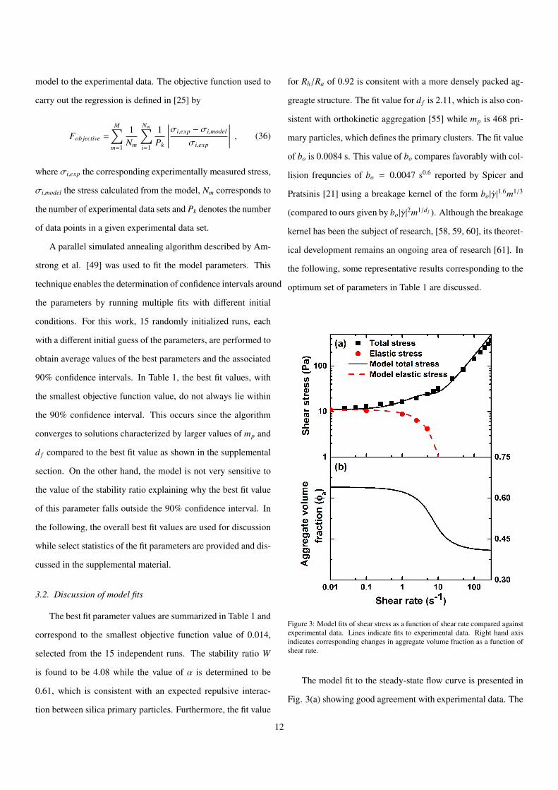
Figure 3: Model fits of shear stress as a function of shear rate compared againstexperimental data. Lines indicate fits to experimental data. Right hand axisindicates corresponding changes in aggregate volume fraction as a function ofshear rate.

The model fit to the steady-state flow curve is presented in

Fig. 3(a) showing good agreement with experimental data. The

12

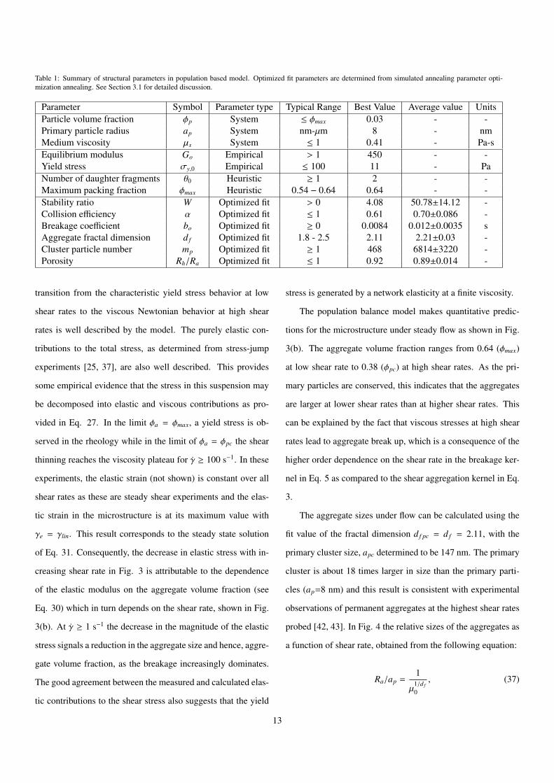
Table 1: Summary of structural parameters in population based model. Optimized fit parameters are determined from simulated annealing parameter opti-mization annealing. See Section 3.1 for detailed discussion.

Parameter Symbol Parameter type Typical Range Best Value Average value UnitsParticle volume fraction φp System ≤ φmax 0.03 - -Primary particle radius ap System nm-µm 8 - nmMedium viscosity µs System ≤ 1 0.41 - Pa-sEquilibrium modulus Go Empirical > 1 450 - -Yield stress σy,0 Empirical ≤ 100 11 - PaNumber of daughter fragments θ0 Heuristic ≥ 1 2 - -Maximum packing fraction φmax Heuristic 0.54 − 0.64 0.64 - -Stability ratio W Optimized fit > 0 4.08 50.78±14.12 -Collision efficiency α Optimized fit ≤ 1 0.61 0.70±0.086 -Breakage coefficient bo Optimized fit ≥ 0 0.0084 0.012±0.0035 sAggregate fractal dimension d f Optimized fit 1.8 - 2.5 2.11 2.21±0.03 -Cluster particle number mp Optimized fit ≥ 1 468 6814±3220 -Porosity Rh/Ra Optimized fit ≤ 1 0.92 0.89±0.014 -

transition from the characteristic yield stress behavior at low

shear rates to the viscous Newtonian behavior at high shear

rates is well described by the model. The purely elastic con-

tributions to the total stress, as determined from stress-jump

experiments [25, 37], are also well described. This provides

some empirical evidence that the stress in this suspension may

be decomposed into elastic and viscous contributions as pro-

vided in Eq. 27. In the limit φa = φmax, a yield stress is ob-

served in the rheology while in the limit of φa = φpc the shear

thinning reaches the viscosity plateau for γ ≥ 100 s−1. In these

experiments, the elastic strain (not shown) is constant over all

shear rates as these are steady shear experiments and the elas-

tic strain in the microstructure is at its maximum value with

γe = γlin. This result corresponds to the steady state solution

of Eq. 31. Consequently, the decrease in elastic stress with in-

creasing shear rate in Fig. 3 is attributable to the dependence

of the elastic modulus on the aggregate volume fraction (see

Eq. 30) which in turn depends on the shear rate, shown in Fig.

3(b). At γ ≥ 1 s−1 the decrease in the magnitude of the elastic

stress signals a reduction in the aggregate size and hence, aggre-

gate volume fraction, as the breakage increasingly dominates.

The good agreement between the measured and calculated elas-

tic contributions to the shear stress also suggests that the yield

stress is generated by a network elasticity at a finite viscosity.

The population balance model makes quantitative predic-

tions for the microstructure under steady flow as shown in Fig.

3(b). The aggregate volume fraction ranges from 0.64 (φmax)

at low shear rate to 0.38 (φpc) at high shear rates. As the pri-

mary particles are conserved, this indicates that the aggregates

are larger at lower shear rates than at higher shear rates. This

can be explained by the fact that viscous stresses at high shear

rates lead to aggregate break up, which is a consequence of the

higher order dependence on the shear rate in the breakage ker-

nel in Eq. 5 as compared to the shear aggregation kernel in Eq.

3.

The aggregate sizes under flow can be calculated using the

fit value of the fractal dimension d f pc = d f = 2.11, with the

primary cluster size, apc determined to be 147 nm. The primary

cluster is about 18 times larger in size than the primary parti-

cles (ap=8 nm) and this result is consistent with experimental

observations of permanent aggregates at the highest shear rates

probed [42, 43]. In Fig. 4 the relative sizes of the aggregates as

a function of shear rate, obtained from the following equation:

Ra/ap =1

µ1/d f

0

, (37)

13

are summarized for steady state conditions. The validity of this

calculation may be independently verified through optical mea-

surements by employing light or neutron scattering (see for ex-

ample [43]).

Figure 4: The calculated relative aggregate size as a function of shear rate usingEq. 37 where ap = 8nm is the primary particle radius.

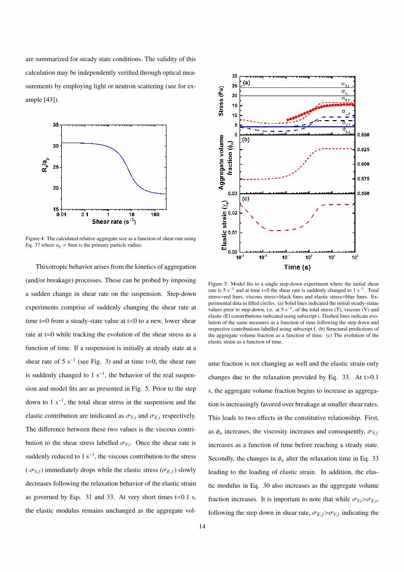
Thixotropic behavior arises from the kinetics of aggregation

(and/or breakage) processes. These can be probed by imposing

a sudden change in shear rate on the suspension. Step-down

experiments comprise of suddenly changing the shear rate at

time t=0 from a steady-state value at t<0 to a new, lower shear

rate at t=0 while tracking the evolution of the shear stress as a

function of time. If a suspension is initially at steady state at a

shear rate of 5 s−1 (see Fig. 3) and at time t=0, the shear rate

is suddenly changed to 1 s−1, the behavior of the real suspen-

sion and model fits are as presented in Fig. 5. Prior to the step

down to 1 s−1, the total shear stress in the suspension and the

elastic contribution are inidicated as σT,i and σE,i respectively.

The difference between these two values is the viscous contri-

bution to the shear stress labelled σV,i. Once the shear rate is

suddenly reduced to 1 s−1, the viscous contribution to the stress

( σV, f ) immediately drops while the elastic stress (σE, f ) slowly

decreases following the relaxation behavior of the elastic strain

as governed by Eqs. 31 and 33. At very short times t<0.1 s,

the elastic modulus remains unchanged as the aggregate vol-

Figure 5: Model fits to a single step-down experiment where the initial shearrate is 5 s−1 and at time t=0 the shear rate is suddenly changed to 1 s−1. Totalstress=red lines, viscous stress=black lines and elastic stress=blue lines. Ex-perimental data in filled circles. (a) Solid lines indicated the initial steady-stataevalues prior to step-down, i.e. at 5 s−1, of the total stress (T), viscous (V) andelastic (E) constributions indicated using subscript i. Dashed lines indicate evo-lution of the same measures as a function of time following the step down andrespective contributions labelled using subscript f. (b) Structural predictions ofthe aggregate volume fraction as a function of time. (c) The evolution of theelastic strain as a function of time.

ume fraction is not changing as well and the elastic strain only

changes due to the relaxation provided by Eq. 33. At t>0.1

s, the aggregate volume fraction begins to increase as aggrega-

tion is increasingly favored over breakage at smaller shear rates.

This leads to two effects in the constitutive relationship. First,

as φa increases, the viscosity increases and consequently, σV, f

increases as a function of time before reaching a steady state.

Secondly, the changes in φa alter the relaxation time in Eq. 33

leading to the loading of elastic strain. In addition, the elas-

tic modulus in Eq. 30 also increases as the aggregate volume

fraction increases. It is important to note that while σV,i>σE,i,

following the step down in shear rate, σE, f>σV, f indicating the

14

role of the percolating network’s elastic stress in dominating

the shear behavior at low shear rates. A key point here is that

thixotropic signatures manifest in σT, f =σE, f +σV, f are clearly

correlated to the time evolution of φa or alternatively µ0.

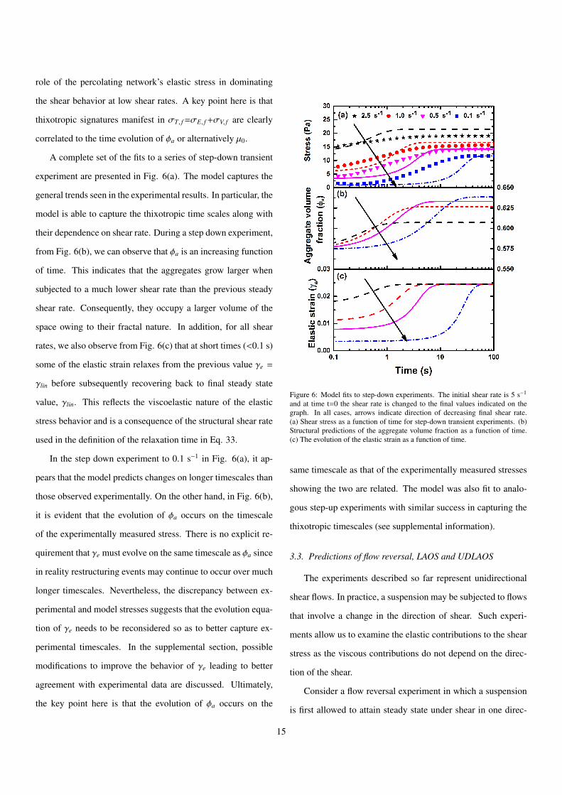
A complete set of the fits to a series of step-down transient

experiment are presented in Fig. 6(a). The model captures the

general trends seen in the experimental results. In particular, the

model is able to capture the thixotropic time scales along with

their dependence on shear rate. During a step down experiment,

from Fig. 6(b), we can observe that φa is an increasing function

of time. This indicates that the aggregates grow larger when

subjected to a much lower shear rate than the previous steady

shear rate. Consequently, they occupy a larger volume of the

space owing to their fractal nature. In addition, for all shear

rates, we also observe from Fig. 6(c) that at short times (<0.1 s)

some of the elastic strain relaxes from the previous value γe =

γlin before subsequently recovering back to final steady state

value, γlin. This reflects the viscoelastic nature of the elastic

stress behavior and is a consequence of the structural shear rate

used in the definition of the relaxation time in Eq. 33.

In the step down experiment to 0.1 s−1 in Fig. 6(a), it ap-

pears that the model predicts changes on longer timescales than

those observed experimentally. On the other hand, in Fig. 6(b),

it is evident that the evolution of φa occurs on the timescale

of the experimentally measured stress. There is no explicit re-

quirement that γe must evolve on the same timescale as φa since

in reality restructuring events may continue to occur over much

longer timescales. Nevertheless, the discrepancy between ex-

perimental and model stresses suggests that the evolution equa-

tion of γe needs to be reconsidered so as to better capture ex-

perimental timescales. In the supplemental section, possible

modifications to improve the behavior of γe leading to better

agreement with experimental data are discussed. Ultimately,

the key point here is that the evolution of φa occurs on the

Figure 6: Model fits to step-down experiments. The initial shear rate is 5 s−1

and at time t=0 the shear rate is changed to the final values indicated on thegraph. In all cases, arrows indicate direction of decreasing final shear rate.(a) Shear stress as a function of time for step-down transient experiments. (b)Structural predictions of the aggregate volume fraction as a function of time.(c) The evolution of the elastic strain as a function of time.

same timescale as that of the experimentally measured stresses

showing the two are related. The model was also fit to analo-

gous step-up experiments with similar success in capturing the

thixotropic timescales (see supplemental information).

3.3. Predictions of flow reversal, LAOS and UDLAOS

The experiments described so far represent unidirectional

shear flows. In practice, a suspension may be subjected to flows

that involve a change in the direction of shear. Such experi-

ments allow us to examine the elastic contributions to the shear

stress as the viscous contributions do not depend on the direc-

tion of the shear.

Consider a flow reversal experiment in which a suspension

is first allowed to attain steady state under shear in one direc-

15

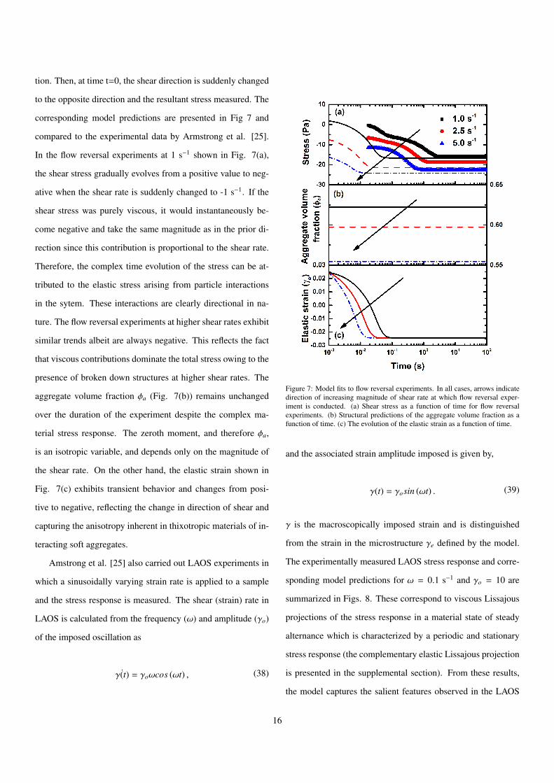
tion. Then, at time t=0, the shear direction is suddenly changed

to the opposite direction and the resultant stress measured. The

corresponding model predictions are presented in Fig 7 and

compared to the experimental data by Armstrong et al. [25].

In the flow reversal experiments at 1 s−1 shown in Fig. 7(a),

the shear stress gradually evolves from a positive value to neg-

ative when the shear rate is suddenly changed to -1 s−1. If the

shear stress was purely viscous, it would instantaneously be-

come negative and take the same magnitude as in the prior di-

rection since this contribution is proportional to the shear rate.

Therefore, the complex time evolution of the stress can be at-

tributed to the elastic stress arising from particle interactions

in the sytem. These interactions are clearly directional in na-

ture. The flow reversal experiments at higher shear rates exhibit

similar trends albeit are always negative. This reflects the fact

that viscous contributions dominate the total stress owing to the

presence of broken down structures at higher shear rates. The

aggregate volume fraction φa (Fig. 7(b)) remains unchanged

over the duration of the experiment despite the complex ma-

terial stress response. The zeroth moment, and therefore φa,

is an isotropic variable, and depends only on the magnitude of

the shear rate. On the other hand, the elastic strain shown in

Fig. 7(c) exhibits transient behavior and changes from posi-

tive to negative, reflecting the change in direction of shear and

capturing the anisotropy inherent in thixotropic materials of in-

teracting soft aggregates.

Amstrong et al. [25] also carried out LAOS experiments in

which a sinusoidally varying strain rate is applied to a sample

and the stress response is measured. The shear (strain) rate in

LAOS is calculated from the frequency (ω) and amplitude (γo)

of the imposed oscillation as

˙γ(t) = γoωcos (ωt) , (38)

Figure 7: Model fits to flow reversal experiments. In all cases, arrows indicatedirection of increasing magnitude of shear rate at which flow reversal exper-iment is conducted. (a) Shear stress as a function of time for flow reversalexperiments. (b) Structural predictions of the aggregate volume fraction as afunction of time. (c) The evolution of the elastic strain as a function of time.

and the associated strain amplitude imposed is given by,

γ(t) = γosin (ωt) . (39)

γ is the macroscopically imposed strain and is distinguished

from the strain in the microstructure γe defined by the model.

The experimentally measured LAOS stress response and corre-

sponding model predictions for ω = 0.1 s−1 and γo = 10 are

summarized in Figs. 8. These correspond to viscous Lissajous

projections of the stress response in a material state of steady

alternance which is characterized by a periodic and stationary

stress response (the complementary elastic Lissajous projection

is presented in the supplemental section). From these results,

the model captures the salient features observed in the LAOS

16

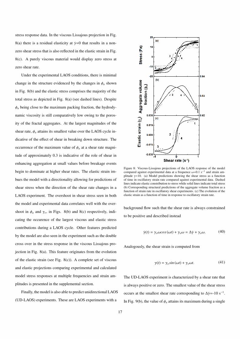
stress response data. In the viscous Lissajous projection in Fig.

8(a) there is a residual elasticity at γ=0 that results in a non-

zero shear stress that is also reflected in the elastic strain in Fig.

8(c). A purely viscous material would display zero stress at

zero shear rate.

Under the experimental LAOS conditions, there is minimal

change in the structure evidenced by the changes in φa shown

in Fig. 8(b) and the elastic stress comprises the majority of the

total stress as depicted in Fig. 8(a) (see dashed lines). Despite

φa being close to the maximum packing fraction, the hydrody-

namic viscosity is still comparatively low owing to the poros-

ity of the fractal aggregates. At the largest magnitudes of the

shear rate, φa attains its smallest value over the LAOS cycle in-

dicative of the effect of shear in breaking down structure. The

occurrence of the maximum value of φa at a shear rate magni-

tude of approximately 0.3 is indicative of the role of shear in

enhancing aggregation at small values before breakage events

begin to dominate at higher shear rates. The elastic strain im-

bues the model with a directionality allowing for predictions of

shear stress when the direction of the shear rate changes in a

LAOS experiment. The overshoot in shear stress seen in both

the model and experimental data correlates well with the over-

shoot in φa and γe, in Figs. 8(b) and 8(c) respectively, indi-

cating the occurence of the largest viscous and elastic stress

contributions during a LAOS cycle. Other features predicted

by the model are also seen in the experiment such as the double

cross over in the stress response in the viscous Lissajous pro-

jection in Fig. 8(a). This feature originates from the evolution

of the elastic strain (see Fig. 8(c)). A complete set of viscous

and elastic projections comparing experimental and calculated

model stress responses at multiple frequencies and strain am-

plitudes is presented in the supplemental section.

Finally, the model is also able to predict unidirectional LAOS

(UD-LAOS) experiments. These are LAOS experiments with a

Figure 8: Viscous-Lissajous projections of the LAOS response of the modelcompared against experimental data at a frequence ω=0.1 s−1 and strain am-plitude γ=10. (a) Model predictions showing the shear stress as a functionof time in oscillatory strain rate compared against experimental data. Dashedlines indicate elastic constribution to stress while solid lines indicate total stress(b) Corresponding structural predictions of the aggregate volume fraction as afunction of strain rate in oscillatory shear experiments. (c) The evolution of theelastic strain as a function of time in response to oscillatory strain rate.

background flow such that the shear rate is always constrained

to be positive and described instead

γ(t) = γoωcos (ωt) + γoω = ∆γ + γoω. (40)

Analogously, the shear strain is computed from

γ(t) = γosin (ωt) + γoωt. (41)

The UD-LAOS experiment is characterized by a shear rate that

is always positive or zero. The smallest value of the shear stress

occurs at the smallest shear rate corresponding to ∆γ=-10 s−1.

In Fig. 9(b), the value of φa attains its maximum during a single

17

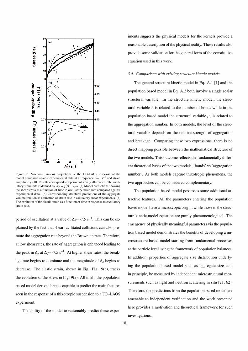
Figure 9: Viscous-Lissajous projections of the UD-LAOS response of themodel compared against experimental data at a frequence ω=1 s−1 and strainamplitude γ=10. Results correspond to a period of steady alternance. The oscil-latory strain rate is defined by ∆γ = ˙γ(t) − γoω. (a) Model predictions showingthe shear stress as a function of time in oscillatory strain rate compared againstexperimental data. (b) Corresponding structural predictions of the aggregatevolume fraction as a function of strain rate in oscillatory shear experiments. (c)The evolution of the elastic strain as a function of time in response to oscillatorystrain rate.

period of oscillation at a value of ∆γ=-7.5 s−1. This can be ex-

plained by the fact that shear facilitated collisions can also pro-

mote the aggregation rate beyond the Brownian rate. Therefore,

at low shear rates, the rate of aggregation is enhanced leading to

the peak in φa at ∆γ=-7.5 s−1. At higher shear rates, the break-

age rate begins to dominate and the magnitude of φa begins to

decrease. The elastic strain, shown in Fig. Fig. 9(c), tracks

the evolution of the stress in Fig. 9(a). All in all, the population

based model derived here is capable to predict the main features

seen in the response of a thixotropic suspension to a UD-LAOS

experiment.

The ability of the model to reasonably predict these exper-

iments suggests the physical models for the kernels provide a

reasonable description of the physical reality. These results also

provide some validation for the general form of the constitutive

equation used in this work.

3.4. Comparison with existing structure kinetic models

The general structure kinetic model in Eq. A.1 [1] and the

population based model in Eq. A.2 both involve a single scalar

structural variable. In the structure kinetic model, the struc-

tural variable λ is related to the number of bonds while in the

population based model the structural variable µ0 is related to

the aggregation number. In both models, the level of the struc-

tural variable depends on the relative strength of aggregation

and breakage. Comparing these two expressions, there is no

direct mapping possible between the mathematical structure of

the two models. This outcome reflects the fundamentally differ-

ent theoretical bases of the two models, ’bonds’ vs ’aggregation

number’. As both models capture thixotropic phenomena, the

two approaches can be considered complementary.

The population based model possesses some additional at-

tractive features. All the parameters entering the population

based model have a microscopic origin, while those in the struc-

ture kinetic model equation are purely phenomenological. The

emergence of physically meaningful parameters via the popula-

tion based model demonstrates the benefits of developing a mi-

crostructure based model starting from fundamental processes

at the particle level using the framework of population balances.

In addition, properties of aggregate size distribution underly-

ing the population based model such as aggregate size can,

in principle, be measured by independent microstructural mea-

surements such as light and neutron scattering in situ [21, 62].

Therefore, the predictions from the population based model are

amenable to independent verification and the work presented

here provides a motivation and theoretical framework for such

investigations.

18

4. Summary and Conclusions

A coarse grained evolution equation for structure dynamics

is developed based on the framework of population balances.

This is achieved by incorporating all the relevant physical pro-

cesses into the rate kernels that describe aggregation-breakage

processes. In addition, by accounting for dynamic arrest, the

structure evolution equation is applicable to aggregating sus-

pensions with a yield stress and can be combined with a con-

stitutive equation for shear stress to provide rheological predic-

tions.

By fitting to a data set for a published, model thixotropic

suspension, it is demonstrated that the population balance based

model captures the experimentally measured rheological be-

havior both qualitatively and quantitatively. This suggests that

a single scalar parameter is a reasonable representation of a

thixotropic suspension for unidirectional flows. However, com-

paring the model predictions to the flow reversal and LAOS

experiments suggests a more accurate constitutive relationship

for the elastic stress is needed for better quantitative agreement.

These experiments demonstrate that directionality, incorporated

into the model through the elastic strain γe, is an important fea-

ture of any candidate thixotropic model. Other improvements in

the constitutive equation may include incorporating additional,

and yet to be accounted for, microscopic variables describing

structural anisotropy to facilitate even better agreement with ex-

periments.

The coarse grained model presented in this work represents

a significant improvement over simple, highly phenomenolog-

ical structural models. In addition to incorporating physically

meaningful parameters, the microscopic model presented in this

work provides a prediction of the aggregation number under

shear flow, which is verifiable using independent structural mea-

surements. The phenomenological and ad hoc nature of struc-

ture kinetic models precludes such a capability. Therefore the

population balance model represents a significant step towards

developing better models to describe structural changes in thixotropic

suspensions under flow.

Nevertheless, the model remains incomplete. In particular,

the coupling of the population balance equation and the stress

expression still needs to be derived from more detailed consid-

erations, including satisfying thermodynamic consistency [63].

Such a development will result in a model that is applicable

to arbitrary flows beyond simple shear. Furthermore, a more

realistic closure approximation can be incorporated such that

aggregate polydispersity can be included. These aspects will be

explored in a future publication. The immediate utility of the

current work is the availability of a microscopically inspired

evolution equation for microstructure that may be applied to

any existing constitutive relationships for thixotropic suspen-

sions that admit a structural variable.

5. Acknowledgements

This material is based upon work supported by the National

Science Foundation under Grant No. CBET 312146. Any opin-

ions, findings or recommendations expressed in this material

are those of the author(s) and do not necessarily reflect the

views of the National Science Foundation.

19

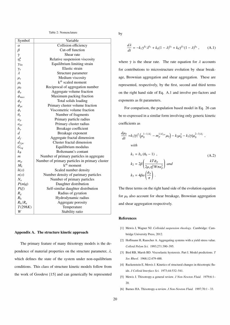
Table 2: Nomenclature

Symbol Variableα Collision efficiencyβ Cut-off functionγ Shear rateηh

r Relative suspension viscosityγlin Equilibrium limiting strainγe Elastic strainλ Structure parameterµs Medium viscosityµk kth scaled momentµ0 Reciprocal of aggregation numberφa Aggregate volume fractionφmax Maximum packing fractionφp Total solids loadingφpc Primary cluster volume fractionφv Viscometric volume fractionθo Number of fragmentsap Primary particle radiusapc Primary cluster radiusbo Breakage coefficientd Breakage exponentd f Aggregate fractal dimensiond f pc Cluster fractal dimensionGeq Equilibrium moduluskB Boltzmann’s contantm Number of primary particles in aggregatemp Number of primary particles in primary clusterMk kth momentn(x) Scaled number densityn(x) Number density of parimary particlesNo Number of primary particlesP(m|q) Daughter distributionP(ξ) Self-similar daughter distributionRg Radius of gyrationRh Hydrodynamic radiusRh/Ra Aggregate porosityT (298K) TemperatureW Stability ratio

Appendix A. The structure kinetic approach

The primary feature of many thixotropy models is the de-

pendence of material properties on the structure parameter, λ,

which defines the state of the system under non-equilibrium

conditions. This class of structure kinetic models follow from

the work of Goodeve [15] and can generically be represented

by

dλdt

= −k1γk2λk3 + k4(1 − λ)k5 + k6γ

k7 (1 − λ)k8 , (A.1)

where γ is the shear rate. The rate equation for λ accounts

for contributions to microstructure evolution by shear break-

age, Brownian aggregation and shear aggregation. These are

represented, respectively, by the first, second and third terms

on the right hand side of Eq. A.1 and involve pre-factors and

exponents as fit parameters.

For comparison, the population based model in Eq. 26 can

be re-expressed in a similar form involving only generic kinetic

coefficients as

dµ0

dt=k1|γ|

2(µ

1−1/d f

0 − m1/d f pcp µ0

)− k2µ

20 − k3|γ|µ

2−3/d f

0 ,

with

k1 = bo (θ0 − 1) ,

k2 = 2β kTφp

2µsηhr Wπa3

p

and

k3 = 4βα(φp

π

).

(A.2)

The three terms on the right hand side of the evolution equation

for µ0 also account for shear breakage, Brownian aggregation

and shear aggregation respectively.

References

[1] Mewis J, Wagner NJ. Colloidal suspension rheology. Cambridge: Cam-

bridge University Press, 2012.

[2] Hoffmann H, Rauscher A. Aggregating systems with a yield stress value.

Colloid Polym Sci. 1993;271:390–395.

[3] Bird RB, Marsh BD. Viscoelastic hysteresis. Part I. Model predictions. T

Soc Rheol. 1968;12:479-488.

[4] Ruckenstein E, Mewis J. Kinetics of structural changes in thixotropic flu-

ids. J Colloid Interface Sci. 1973;44:532–541.

[5] Mewis J. Thixotropy-a general review. J Non-Newton Fluid. 1979;6:1–

20.

[6] Barnes HA. Thixotropy-a review. J Non-Newton Fluid. 1997;70:1 - 33.

20

[7] Mewis J, Wagner NJ. Thixotropy. Adv Colloid Interface Sci.

2009;147:214–227.

[8] Boger DV. Rheology and the resource industries. Chem Eng Sci.

2009;64:4525–4536.

[9] Chang C, Smith PA. Flow-induced structure in a system of nuclear waste

simulant slurries. Rheol Acta. 1996;35:382–389.

[10] Thareja P, Golematis A, Street CB, et al. Influence of surfactants on the

rheology and stability of crystallizing fatty acid pastes. J Am Oil Chem

Soc. 2013;90:273–283.

[11] Natan B, Rahimi S. The status of gel propellants in year 2000. Int J Ener-

getic Materials Chem Prop. 2002;5.

[12] Green H, Weltmann R. Analysis of Thixotropy of Pigment-Vehicle

Suspensions-Basic Principles of the Hysteresis Loop. Ind Eng Chem.

1943;15:201–206.

[13] Hahn SJ, Ree T, Eyring H. Flow mechanism of thixotropic substances.

Ind Eng Chem. 1959;51:856–857.

[14] Apostolidis AJ, Armstrong MJ, Beris AN. Modeling of human blood rhe-

ology in transient shear flows. J Rheol. 2015;59:275-298.

[15] Goodeve CF. A general theory of thixotropy and viscosity. Trans. Faraday

Soc.. 1939;35:342–358.

[16] Dullaert K, Mewis J. A structural kinetics model for thixotropy. J Non-

Newton Fluid. 2006;139:21 - 30.

[17] Randolph AD, Larson MA. Transient and steady state size distributions

in continuous mixed suspension crystallizers. AIChE J. 1962;8:639–645.

[18] Hulburt HM, Katz S. Some problems in particle technology: A statistical

mechanical formulation. Chem Eng Sci. 1964;19:555–574.

[19] Von Smoluchowski M. Versuch einer mathematischen theorie der koagu-

lationskinetik kolloider losungen. Zeit Phys Chem. 1917;92:129-168.

[20] Flesch Jurgen C, Spicer PT, Pratsinis SE. Laminar and turbulent shear-

induced flocculation of fractal aggregates. AIChE J. 1999;45:1114–1124.

[21] Spicer P, Pratsinis SE. Coagulation and fragmentation: Universal steady-

state particle-size distribution. AIChE J. 1996;42:1612–1620.

[22] Von Smoluchowski M. Three discourses on diffusion, Brownian move-

ments, and the coagulation of colloid particles. Phys. Z. Sowjet.

1916;17:557–571.

[23] Barthelmes G, Pratsinis SE, Buggisch H. Particle size distributions and

viscosity of suspensions undergoing shear-induced coagulation and frag-

mentation. Chem Eng Sci. 2003;58:2893-2902.

[24] Mohtaschemi M, Puisto A, Illa X, Alava MJ. Rheology dynamics of ag-

gregating colloidal suspensions. Soft matter. 2014;10:2971–2981.

[25] Armstrong MJ, Beris AN, Rogers SA, Wagner NJ. Dynamic shear rheol-

ogy of a thixotropic suspension: Comparison of an improved structure-

based model with large amplitude oscillatory shear experiments. J Rheol.

2016;60:433-450.

[26] Dullaert K, Mewis J. A model system for thixotropy studies. Rheol Acta.

2005;45:23–32.

[27] Meakin Paul. Fractal aggregates. Adv Colloid Interface Sci.

1987;28:249–331.

[28] Ramkrishna D. Population balances: Theory and applications to partic-

ulate systems in engineering. San Diego, CA: Academic Press, 2000.

[29] Fuchs N. Uber die Stabilitat und Aufladung der Aerosole. Z Phys.

1934;89:736–743.

[30] Thomas DN, Judd SJ, Fawcett N. Flocculation modelling: a review. Water

Res. 1999;33:1579–1592.

[31] Marchisio DL, Fox RO. Computational models for polydisperse partic-

ulate and multiphase systems. Cambridge: Cambridge University Press,

2013.

[32] Diemer RB, Olson JH. A moment methodology for coagulation and

breakage problems: Part 1-analytical solution of the steady-state popu-

lation balance. Chem Eng Sci. 2002;57:2193 - 2209.

[33] Diemer RB, Olson JH. A moment methodology for coagulation and

breakage problems: Part 2-moment models and distribution reconstruc-

tion. Chem Eng Sci. 2002;57:2211 - 2228.

[34] Sommer M, Stenger F, Peukert W, Wagner NJ. Agglomeration and break-

age of nanoparticles in stirred media millsa comparison of different meth-

ods and models. Chem Eng Sci. 2006;61:135–148.

[35] Kruis FE, Kusters KA, Pratsinis SE, Scarlett B. A simple model for the

evolution of the characteristics of aggregate particles undergoing coagu-

lation and sintering. Aerosol Sci Technol. 1993;19:514–526.

[36] Vemury S, Kusters KA, Pratsinis SE. Time-lag for attainment of the self-

preserving particle size distribution by coagulation. J Colloid Interface

Sci. 1994;165:53–59.

[37] Dullaert K, Mewis J. Stress jumps on weakly flocculated dispersions:

Steady state and transient results. J Colloid Interface Sci. 2005;287:542

- 551.

[38] Lewis TB, Nielsen LE. Viscosity of dispersed and aggregated suspensions

of spheres. T Soc Rheol. 1968;12:421–443.

[39] Russel WB, Wagner NJ, Mewis J. Divergence in the low shear viscosity

for Brownian hard-sphere dispersions: At random close packing or the

glass transition? J Rheol. 2013;57:1555–1567.

[40] Faroughi SA, Huber C. A generalized equation for rheology of emulsions

and suspensions of deformable particles subjected to simple shear at low

Reynolds number. Rheol Acta. 2015;54:85–108.

[41] Maron SH, Pierce PE. Application of Ree-Eyring generalized flow theory

to suspensions of spherical particles. J Colloid Sci. 1956;11:80–95.

[42] Dullaert K. Constitutive Equations for Thixotropic Dispersions, Ph.D.

21

Thesis, Katholieke Universiteit Leuven, Leuven, Belgium, 2005.

[43] Armstrong M. Investigating and modeling thixotropic behavior, mi-

crostructure and rheology of complex material, Ph.D. Thesis, University

of Delaware, Newark, Delaware, 2015.

[44] Potanin AA, De Rooij R, Ende D, Mellema J. Microrheological modeling

of weakly aggregated dispersions. J Chem Phys. 1995;102:5845-5853.

[45] Hsiao LC, Newman RS, Glotzer SC, Solomon MJ. Role of isostaticity and

load-bearing microstructure in the elasticity of yielded colloidal gels. Pro-

ceedings of the National Academy of Sciences. 2012;109:16029–16034.

[46] Russel WB. Theoretical approaches to the rheology of concentrated dis-

persions. Powder Technol. 1987;51:15–25.

[47] Shih WH, Shih WY, Kim SI, Liu J, Aksay IA. Scaling behavior of the

elastic properties of colloidal gels. Phys Rev A. 1990;42:4772.

[48] Dimitriou CJ, Ewoldt RH, McKinley GH. Describing and prescribing the

constitutive response of yield stress fluids using large amplitude oscilla-

tory shear stress (LAOStress). J Rheol. 2013;57:27-70.

[49] Armstrong MJ, Beris AN, Wagner NJ. An Adaptive Parallel Tempering

Method for the Dynamic Data-Driven Parameter Estimation of Nonlinear

Models (submitted). AIChE J. 2016.

[50] Curtis ASG, Hocking LM. Collision efficiency of equal spherical particles

in a shear flow. The influence of London-van der Waals forces. Trans.

Faraday Soc.. 1970;66:1381-1390.

[51] Riseman J, Kirkwood JG. The Intrinsic Viscosity, Translational and Ro-

tatory Diffusion Constants of Rod-Like Macromolecules in Solution. J

Chem Phys. 1950;18:512–516.

[52] Meakin P, Chen ZY, Deutch JM. The translational friction coefficient

and time dependent cluster size distribution of three dimensional cluster–

cluster aggregation. J Chem Phys. 1985;82:3786–3789.

[53] Lattuada M, Wu H, Morbidelli M. Hydrodynamic radius of fractal clus-

ters. J Colloid Interface Sci. 2003;268:96–105.

[54] Weitz DA, Huang JS, Lin MY, Sung J. Limits of the fractal dimen-

sion for irreversible kinetic aggregation of gold colloids. Phys Rev Lett.

1985;54:1416.

[55] Oles V. Shear-induced aggregation and breakup of polystyrene latex par-

ticles. J Colloid Interface Sci. 1992;154:351–358.

[56] Reerink H, Overbeek JG. The rate of coagulation as a measure of the

stability of silver iodide sols. Discuss Faraday Soc. 1954;18:74–84.

[57] Russel WB, Saville DA, Schowalter WR. Colloidal dispersions. Cam-

bridge: Cambridge University Press, 1992.

[58] Adler PM, Mills PM. Motion and Rupture of a Porous Sphere in a Linear

Flow Field. J Rheol. 1979;23:25-37.

[59] Sonntag RC, Russel WB. Structure and breakup of flocs subjected to fluid

stresses: II. Theory. J Colloid Interface Sci. 1987;115:378 - 389.

[60] Higashitani K, Iimura K. Two-Dimensional Simulation of the Breakup

Process of Aggregates in Shear and Elongational Flows. J Colloid Inter-

face Sci. 1998;204:320 - 327.

[61] Harshe YM, Lattuada M. Breakage Rate of Colloidal Aggregates in Shear

Flow through Stokesian Dynamics. Langmuir. 2012;28:283-292. PMID:

22122803.

[62] Sandkuhler P, Sefcik J, Lattuada M, Wu H, Morbidelli M. Modeling struc-

ture effects on aggregation kinetics in colloidal dispersions. AIChE J.

2003;49:1542–1555.

[63] Larson RG. Constitutive equations for thixotropic fluids. J Rheol.

2015;59:595–611.

22