A Conic Integer Programming Approach to Stochastic Joint … · 2018-08-16 · mixed-integer...

OPERATIONS RESEARCHVol. 60, No. 2, March–April 2012, pp. 366–381ISSN 0030-364X (print) � ISSN 1526-5463 (online) http://dx.doi.org/10.1287/opre.1110.1037

© 2012 INFORMS

A Conic Integer Programming Approach toStochastic Joint Location-Inventory Problems

Alper Atamtürk, Gemma Berenguer, Zuo-Jun (Max) ShenDepartment of Industrial Engineering and Operations Research, University of California, Berkeley, Berkeley, California 94720

{[email protected], [email protected], [email protected]}

We study several joint facility location and inventory management problems with stochastic retailer demand. In particular,we consider cases with uncapacitated facilities, capacitated facilities, correlated retailer demand, stochastic lead times, andmulticommodities. We show how to formulate these problems as conic quadratic mixed-integer problems. Valid inequalities,including extended polymatroid and extended cover cuts, are added to strengthen the formulations and improve the com-putational results. Compared to the existing modeling and solution methods, the new conic integer programming approachnot only provides a more general modeling framework but also leads to fast solution times in general.

Subject classifications : integrated supply chain; risk pooling; conic mixed-integer program; polymatroids; covers.Area of review : Transportation.History : Received December 2010; revisions received July 2011, October 2011; accepted November 2011.

1. IntroductionTo achieve significant cost savings across the supply chain,the major cost components that can impact the performanceof the supply chain should be considered jointly rather thanin isolation. This is not only true for decisions at the samehierarchical level (for instance, it is well known that theinventory management scheme and the transportation strat-egy should be integrated) but also at different levels.

Recently, we have seen a proliferation of research on inte-grated facility location and inventory management models.These models simultaneously consider decisions at both thestrategic (location decisions) level and tactical (inventorydecisions) level. Daskin et al. (2002) and Shen et al. (2003)were the first to propose joint location-inventory modelswith nonlinear safety stock costs and integer location deci-sions. The nonlinearity arises from the risk pooling strategyused to buffer random demand at the retailers. Specifically,they consider the design of a supply chain system in whicha supplier ships products to a set of retailers, each withuncertain demand. The decision problem is to determinehow many distribution centers to locate, where to locatethem, which retailers to assign to each distribution center(DC), how often to reorder at the distribution center, andwhat level of safety stock to maintain to minimize totallocation, shipment, and inventory costs while ensuring aspecified level of service.

The complexity of integrated models with integer deci-sion variables and nonlinear costs and constraints suggestedthe development of special-purpose heuristic algorithms forvarious special cases. Shen et al. (2003) outline a columngeneration approach while Daskin et al. (2002) proposea Lagrangian relaxation approach for this problem. Both

of the approaches utilize a low-order polynomial algo-rithm for solving a nonlinear (concave) integer subprob-lem. Özsen et al. (2008) study a capacitated version of thejoint location-inventory problem, and they design an effi-cient algorithm to handle fractional terms in the objectivefunction and nonlinear capacity constraints.

In this paper we propose a new flexible and generalapproach based on recent developments in conic integer pro-gramming. In particular, we reformulate the joint location-inventory models with different types of nonlinearities asconic quadratic mixed-integer programs, which can then besolved directly using standard optimization software pack-ages without the need for designing specialized algorithms.This approach has several advantages over the Lagrangianrelaxation and column generation approaches. For the laterapproaches to work well, one needs to design special-purpose algorithms for solving the nonlinear sub-problemsand, for their exact solutions, implement a specializedbranch-and-bound algorithm that either makes use of theLagrangian relaxation bounds or allows convenient gener-ation of columns in the search tree. In many cases, thisrequires an extensive programming effort which often givesway to simpler heuristics approaches as alternative. More-over, these special-purpose algorithms often work undersimplifying assumptions on the problems and are not eas-ily extendable to more general settings. On the other hand,as we will see in the later discussions, our proposed conicquadratic programming based approach is direct, efficient,and flexible enough to handle more general problems thathave been considered before in the literature, including cor-related retailer demand, stochastic lead times, and multi-commodity cases.

366

Atamtürk, Berenguer, and Shen: Joint Location-Inventory ProblemsOperations Research 60(2), pp. 366–381, © 2012 INFORMS 367

The main contributions in this paper can be summarizedas follows:

1. We propose a new approach to modeling and solvingintegrated supply chain problems with stochastic demand.The conic integer programming based approach is general,flexible, and efficient.

2. We show how to reformulate different types of non-linearities arising in joint location-inventory problems asconic quadratic integer programs.

3. We address for the first time the joint location-inventory problems with distinct variance-to-mean ratio foreach retailer, correlated retailer demand, stochastic leadtimes, and correlated multicommodity demand.

4. We strengthen the conic quadratic integer formula-tions with cutting planes for their efficient solution.

5. We perform computational studies, comparing thenew approach with earlier ones in the literature that dealwith special cases of our general model, and investigate theimpact of correlated demand on the supply chain design.

The rest of the paper is organized as follows. In §2we review the relevant literature on integrated location andinventory optimization and recent developments in conicprogramming. In §3 we formally define a conic quadraticmixed-integer program and review the notation and param-eters used in the paper. In §4 we address the basic unca-pacitated model and give a conic quadratic mixed-integerformulation for it. In §5 we study the capacitated model andits respective equivalent conic mixed-integer reformulation.In these two sections, we also show how to utilize rele-vant polymatroid and cover inequalities for strengtheningthe conic quadratic formulations. In §6 we generalize themodels to incorporate correlated retailer demand, stochasticlead times, and multicommodities. Each model is accompa-nied by its equivalent conic quadratic formulation. In §7 wepresent our computational results with the conic quadraticMIP approach, provide comparisons with earlier studies,and investigate the impact of correlations and stochasticlead times. Finally, in §8 we conclude with a few finalremarks.

2. Literature ReviewIn this section we review the literature on integrated sup-ply chain design models, especially the papers that modelfixed location costs and nonlinear inventory costs. We men-tion some work related to multicommodity in supply chaindesign and retailers’ and products’ demand correlation.Recent developments on conic integer programming arealso reviewed.

Daskin et al. (2002) and Shen et al. (2003) proposethe first location-inventory model with nonlinear inventorycosts. They propose Lagrangian relaxation and column gen-eration methods for its solution, respectively. Both methodsemploy the same subproblem, which is solved in O4n logn5for two special cases: when the variance of the demand isproportional to the mean (as in the Poisson demand case),

or when the demand is deterministic. In these cases theobjective function simplifies to one with a single nonlinear(concave) term for each retailer, which underlies the effi-cient solution approach. Shu et al. (2005) and Shen and Qi(2007) study more general models in which these assump-tions on demand are relaxed. As a result, multiple nonlinearterms appear in the objective functions. Specifically, Shuet al. (2005) study a subproblem with two concave termsand Shen and Qi (2007) added a third term to accommo-date routing costs. More general problems are studied byQi and Shen (2007), Shen (2005), Shen and Daskin (2005),and Snyder et al. (2007).

Özsen et al. (2008) consider the capacitated version ofthe models in Shen et al. (2003) and Daskin et al. (2002).They propose a Lagrangian relaxation based solution algo-rithm to solve the problem, where the Lagrangian subprob-lems are nonlinear integer program which include concaveand fractional terms. For more detailed review on inte-grated location-inventory models, we refer the reader toShen (2007).

Multicommodity problems have been studied in the loca-tion literature and are of our interest for the present paper.Geoffrion and Graves (1974) utilize a Bender’s decompo-sition to solve multicommodity problems with capacitatedplants and DCs. Dasci and Verter (2001) consider eco-nomies of scale by introducing concave technology selec-tion cost into the objective function of a multicommoditylocation model. To handle concavity of the objective func-tion, they solve the problem with a series of piecewise linearunderestimations. In the integrated supply chain design lit-erature, Shen (2005) presents a multicommodity model thatincludes economies of scale cost terms in the objective func-tion. The author proposes a Lagrangian relaxation solutionalgorithm with a low-order polynomial algorithm to solvethe Lagrangian relaxation subproblems.

Correlated demand has received much attention in theinventory management literature, and it can be studiedacross time, sites, and products. Johnson and Thompson(1975) are among the first to study correlated demand in asingle item and a single location setting. Erkip et al. (1990)consider a multi-echelon inventory system where demand isa first-order autoregressive process and is correlated acrosssites and time. These authors solve for the optimal safetystock level and show the impact of demand correlation overtime. Charnes et al. (1995) assume that the sequence ofdemand is a covariance-stationary Gaussian stochastic pro-cess. The literature on supply chain problems with correla-tion between different products is scarce. Inderfurth (1991)studies the effects of correlation between different itemson the optimal safety stock in stochastic multi-stage pro-duction/distribution systems. Fine and Freund (1990) andGoyal and Netessine (2011) study the correlation betweenproducts in the context of product and volume flexibility.

Recently, there has been a number of advances in the the-ory of conic integer programming. Atamtürk and Narayanan(2010) give conic mixed-integer rounding inequalities for

Atamtürk, Berenguer, and Shen: Joint Location-Inventory Problems368 Operations Research 60(2), pp. 366–381, © 2012 INFORMS

conic quadratic mixed-integer programs and Çezik andIyengar (2005) give convex quadratic cuts for mixed 0-1conic programs. Atamtürk and Narayanan (2011) proposelifting methods for conic mixed-integer programming.Atamtürk and Narayanan (2009) propose cover-typeinequalities for submodular knapsack sets and Atamtürkand Narayanan (2008) introduce polymatroid inequalitiesthat can help with solving special structured conic quadraticprograms efficiently. We have utilized these recently intro-duced valid inequalities for the efficient solution of our jointlocation-inventory models.

3. PreliminariesA conic quadratic mixed-integer program (CQMIP) is anoptimization problem of the form

min c′x1

s.t. �Aix+ bi�2 ¶ d′

ix+ ei1 i = 11 0 0 0 1 p1

where x ∈ �n × �m, � · �2 is the Euclidean norm and allparameters are rational. Observe that a linear constraint canbe written as a special case of a conic quadratic constraintby letting Ai = bi = 0. Similarly, a convex quadratic con-straint can be written as a special case by letting d′

i = 0.For an introduction to (convex) conic quadratic program-ming we refer the reader to Ben-Tal and Nemirovski (2001)and Alizadeh and Goldfarb (2003). In recent years therehave been significant developments on the computation ofconic quadratic mixed-integer programs. Due to the rise indemand for solution of CQMIP, commercial optimizationsoftware vendors such as CPLEX and Mosek have added totheir offerings branch-and-bound based solvers for CQMIP.

During the last decade, conic quadratic programs havebeen employed to solve problems in different areas suchas portfolio optimization, scheduling, and energy planning.Indeed, basic uncapacitated facility location problems havebeen formulated as conic quadratic programs (e.g., Kuoand Mittelmann 2004). In this paper, we show how tomodel nonlinear mixed 0-1 optimization models arising incomplex supply chain design problems as conic quadraticmixed 0-1 programs and utilize the recent advances in cut-ting planes for their scalable solution.

The following parameters and notation are used through-out the paper:

Demand�i: mean of daily demand at retailer i,�i: standard deviation of daily demand at retailer i,V : variance-covariance matrix of daily demand at

retailers.Costsdij : unit cost of shipment between retailers i and j ,fj : annualized fixed cost of locating a DC at retailer

site j,Fj : fixed cost of placing an order at DC j,aj : unit cost of shipment from the central plant to DC j,

gj : fixed cost per shipment from the central plant to DC j,h: unit inventory holding cost per year.Weights�: weight associated with the transportation costs,�: weight associated with the inventory costs.Other parameters�: days worked per year,�: service level,z�: standard normal deviation associated with service

level �,Lj : lead time in days at DCj .Decision variables

xj =

11 if a distribution center (DC) is located at

retailer site j1

01 otherwise3

yij =

11 if retailer i is assigned to DC located at

retailer site j1

01 otherwise0

4. Model with Uncapacitated FacilitiesWe start with the basic uncapacitated location-inventorymodel, which was originally studied by Daskin et al. (2002)and Shen et al. (2003). Their model assumes the following:

• Shipments are direct from DCs to retailers.• Demand at each retailer is independent and Gaussian.• Each retailer is supplied from exactly one DC.

4.1. Model 1

Under the assumptions listed above, the joint location-inventory model is formulated as follows:

min∑

j∈J

(

fjxj +∑

i∈I

dijyij +Kj

√

∑

i∈I

�iyij

+ qj

√

∑

i∈I

�2i yij

)

1

4P15 s.t.∑

j∈J

yij = 11 i ∈ I1 (1)

yij ¶ xj1 i ∈ I1 j ∈ J 1 (2)

xj1 yij ∈ 801191 i ∈ I1 j ∈ J 1 (3)

where dij = ��4dij + aj5�i, Kj =√

2�h4Fj +�gj5�, andqj = z��

√

Ljh.The objective of (P1) is to minimize total expected

cost of location, shipment, and inventory management.The first objective term is the fixed cost of locating DCj , fjxj . The second term is the cost of shipping fromDC j to the retailers and from the central plant to DC j ,��

∑

i∈I4dij +aj5�iyij . The third term captures the workinginventory effects due to the fixed costs of placing orders


and the fixed costs of shipping from the central plant toDC j ,

√

2�h4Fj +�gj5�√

∑

i∈I �iyij . The fourth term is the

expected safety stock cost at DC j , z��√

Ljh√

∑

i∈I �2i yij .

Appendix A supplies the derivation of the working inven-tory term.

Constraints (1) ensure that each retailer is assigned toexactly one DC. Constraints (2) guarantee that retailersare only assigned to open DCs. Constraints (3) define thedomain of the decision variables.

As mentioned in the literature review, in order to handlethe nonlinearity of the objective, Shen et al. (2003) solve(P1) by transforming it into a set-covering model and solveit using column generation approach, where the columnsare generated by solving an unconstrained nonlinear sub-problem on binary variables. Daskin et al. (2002) solve thesame problem by designing a Lagrangian relaxation algo-rithm. In both of these papers the ratio of the demand vari-ance to the mean demand is assumed to be constant forall retailers (�2

i /�i = � ∀ i). Under this assumption, (P1)would have only one square root term instead of two foreach retailer, which makes the Lagrangian and column gen-eration subproblems easier to solve. Our approach does notrequire this assumption.

4.2. A Conic Quadratic MIP Formulation

In this section we show how to reformulate (P1) as a conicquadratic mixed-integer program (CQMIP). The advantageof the CQMIP formulation is that it can be solved directlyusing standard optimization software packages such asCPLEX or Mosek.

By introducing auxiliary variables t1j1 t2j ¾ 0 to representthe nonlinear terms in the objective and using the fact thatyij = y2

ij , we reformulate (P1) as

min∑

j∈J

(

fjxj +∑

i∈I

dijyij +Kj t1j + qj t2j

)

1

4CQMIP15 s.t.∑

i∈I

�iy2ij ¶ t2

1j1 j ∈ J 1 (4)

∑

i∈I

�2i y

2ij ¶ t2

2j1 j ∈ J 1 (5)

t1j1 t2j ¾ 01 j ∈ J 1 (6)

415–4350

Note that the objective of (CQMIP1) is linear and theconstraints are either conic quadratic or linear, which fitsinto the general conic quadratic mixed-integer program-ming model described in §3.

4.3. Polymatroid Inequalities

Commercial software packages utilize a branch-and-boundalgorithm for solving conic quadratic MIPs, and their per-formance can be significantly improved by strengthening theformulations with structural cutting planes. In this section,

utilizing submodularity, we will reformulate constraints (4)and (5) with polymatroid inequalities of Atamtürk andNarayanan (2008) to strengthen the convex relaxation ofCQMIP1.

Definition 1. A function g2 2I → � is submodular ifg4S ∪ i5 − g4S5 ¾ g4T ∪ i5 − g4T 5 for all S ⊆ T ⊆ I andi ∈ I\T .

Definition 2. For a submodular function g, thepolyhedron

EPg ={

� ∈�I 2 �4S5¶ g4S51 ∀S ⊆ I}

is called an extended polymatroid.

For an extended polymatroid EPg , Atamtürk andNarayanan (2008) show that the linear inequality

�y ¶ t with � ∈EPg

is valid for the lower convex envelope of g:

Qg 2= conv{

4y1 t5 ∈ 80119�I �×�2 g4y5¶ t

}

0

Because tj ¾ 0, ∀ j ∈ J and y2ij = yij , ∀ i ∈ I1 j ∈ J ,

inequalities∑

i∈I �iy2ij ¶ t2

j and√

∑

i∈I �iyij ¶ tj are equiv-alent. The latter inequalities have a submodular form due tothe concavity of the square root function and the nonneg-ativity of the arguments in the square root function. Moreprecisely, the set function

g4S5 2=√

∑

i∈S

�i1 ∀S ⊆ I

is submodular.Although there are exponentially many extremal (corre-

sponding to extreme points � of EPg) extended polyma-troid inequalities, only a small subset of them is needed inthe branch-and-bound search tree. It turns out that, givena solution, finding a violated polymatroid cut can be doneeasily. Formally, the separation problem for the extendedpolymatroid inequalities is defined as follows:

Given 4y∗1 t∗5 ∈ 60117�I � ×�+, let

� = max8�y∗2 � ∈EPg90

If � > t∗, then the extended polymatroid inequality �∗x¶ t

for an optimal �∗ cuts off 4y∗1 t∗5; otherwise, there existsno violated extended polymatroid inequality. Thus, theseparation problem is an optimization over an extendedpolymatroid, which is solved by the greedy algorithm ofEdmonds (1970). For completeness we describe the algo-rithm in Appendix B.


5. Model with Capacitated FacilitiesIn this section we consider the generalization of (P1) withfacility capacities and show how to reformulate it as a conicquadratic MIP. Özsen et al. (2008) present a generalizationof the integrated inventory-location model (P1) by intro-ducing inventory capacity constraints for the DCs. Theseconstraints are defined for a 4Q1 r5 inventory control policywith type-I service level. Compared with model (P1), theirmodel contains additional nonlinear terms:

• Nonlinear (concave) capacity constraints for each DC,• Nonlinear (fractional) terms in the objective function.As in the uncapacitated counterparts of Daskin et al.

(2002) and Shen et al. (2003), in order to simplify the prob-lem, Özsen et al. (2008) also assume the variance of eachretailer’s demand to be proportional to the mean demand.In particular, �2

i =�i ∀ i. We do not make this assumptionhere.

5.1. Model 2

Let Cj be the maximum inventory capacity of DC j andQj be the reorder quantity for DC j . Then, the integratedinventory-location model with capacitated facilities is for-mulated as the following nonlinear mixed 0-1 optimizationproblem:

4P25

min∑

j∈J

(

fjxj +∑

i∈I

dijyij + Fj

∑

i∈I �iyij

Qj

+qj

√

∑

i∈I

�2i yij + �h

Qj

2

)

1

s.t. Qj + z�

√

Lj

√

∑

i∈I

�2i yij +Lj

∑

i∈I

�iyij ¶Cj1

j ∈ J 1 (7)

Qj ¾ 01 j ∈ J 1 (8)

415–4351

where Fj = 4Fj +�gj5�.The third term in the objective is the expected fixed cost

of placing an order at DC j and the expected fixed cost pershipment from the central plant to DC j . The fifth term isnew; it is the average inventory holding cost at DC j .

Constraints (7) define the capacity of each DC to bethe sum of the order quantity Qj and the reorder point.Note that in defining the DC capacity, we consider theworst-case scenario, i.e., no demand is observed duringlead time. The reorder point is the sum of the safety stock,

z�√

Lj

√

∑

i∈I �2i yij , and the expected demand during lead

time, Lj

∑

i∈I �iyij .

5.2. An Equivalent Conic Quadratic MIP Model

The objective of (P2) is neither concave nor convex. Özsenet al. (2008) develop a Lagrangian relaxation based heuris-tic algorithm to solve this problem. In this section we show

how to transform (P2) into the following equivalent conicquadratic MIP, which leads to an exact solution of the prob-lem. Consider

4CQMIP25

min∑

j∈J

(

fjxj +∑

i∈I

dijyij + qj tj +�

2hzj

)

1

s.t. Qj + z�

√

Lj tj +Lj

∑

i∈I

�iyij ¶Cjxj1 j ∈ J 1 (9)

∑

i∈I

�2i y

2ij ¶ t2

j 1 ∀ j ∈ J 1 (10)

∑

i∈I

Hj�iy2ij +

(

Qj −zj

2

)2

−z2j

4¶ 01 j ∈ J 1 (11)

tj1 zj ¾ 01 j ∈ J 1 (12)

415–4351 4851

where Hj = Fj/44�h5/25.Constraints (1)–(3), and (8) are still present in the trans-

formed problem. Constraints (7) are linearized as (9). Anauxiliary variable tj is introduced for each j and definedby the constraints (10). Constraints (9) have stronger righthand sides than constraints 475. We linearize the objectiveby using tj and the auxiliary variables for zj for each j .Variables zj are defined by the constraints (11) and (12).

Proposition 1. Problem (P2) is equivalent to (CQMIP2).

Proof. Variables tj and constraint (10) are used to sub-

stitute the terms√

∑

i∈I �2i yij as in (MIPCQ1). The sec-

ond substitution for the third and fifth inventory terms4∑

i∈I �iyij5/Qj +Qj follows from the following identities:∑

i∈I �iyiQ

+Q¶ z ⇔∑

i∈I

�iyi +Q2 ¶Qz 4as Q> 05

⇔∑

i∈I

�iy2i +Q2 ¶Qz 4as yi = y2

i 5

⇔∑

i∈I

�iy2i +

(

Q−z

2

)2

¶ z2

40 �

5.3. Extended Cover Cuts

To strengthen formulation (CQMIP2) we add cover typeinequalities derived from nonlinear knapsack relaxations ofthe formulation. Toward this end, consider the capacity con-straints (9). For each j, we relax the left-hand side of theconstraint by dropping Qj . Furthermore, we substitute tjwith the left-hand side of constraint (10) to arrive at thenonlinear 0-1 knapsack constraint

z�

√

Lj

√

∑

i∈I

�2i yij +Lj

∑

i∈I

�iyij ¶Cj 0 (13)

For simplicity of notation, we drop the subscript j todefine the inequalities. For inequality (13), define the setfunction f 2 2I →�, where

f 4S5= z�√L√

�24S5+L�4S51


�24S5 2=∑

i∈S �2i and �4S5 2=

∑

i∈S �i. Using submodular-ity of f , Atamtürk and Narayanan (2009) give cover andextended cover cuts for the submodular knapsack set,

Y = 8y ∈ 80119�I �2 f 4y5¶C9

=

{

y ∈ 80119�I �2 z�√L√

∑

i∈I

�2i yi +L

∑

i∈I

�iyi ¶C

}

0

They show that given a subset of indices S ⊆ I and theconic quadratic 0-1 knapsack set Y , we can find valid coverinequalities that depend on the cover set.

Definition 3. S ⊆ I is called a cover for Y ifz�

√L√

�24S5+L�4S5 > C.

Atamtürk and Narayanan (2009) show that for cover Sthe corresponding cover inequality∑

i∈S

yi ¶ �S� − 1

is valid for Y .As with polymatroid inequalities, a separation algorithm

generates the cover constraints at the root node of thebranch-and-bound tree for each j . Given y∗ ∈ 60117�I � a vio-lated cover inequality can be found by solving the follow-ing nonlinear 0-1 separation problem:

� = min{

y′z2 z�√L√

∑

i∈I

�2i zi+L

∑

i∈I

�izi>C1z∈80119�I �

}

1

where y = 1 − y∗. If � < 1, then the cover inequality cor-responding to optimal z cuts off y∗. We employ a heuristicalgorithm based on rounding the convex relaxation of theseparation as proposed in Atamtürk and Narayanan (2009).For completeness, this algorithm is stated in Appendix C.

Cover inequalities can be strengthened by extendingthem with noncover variables. To introduce extended coverinequalities, we first need to define the difference functionand the notion of extension.

Definition 4. Given a set function f on I and i ∈ I , thedifference function � is defined as �i4S5 2= f 4S∪ i5− f 4S5for S ⊆ I\i.

Definition 5. Let � = 4k4151 0 0 0 1 k4�I �−�S�55 be a permuta-tion of the indices in I\S. Define S` = S ∪ 8k4151 0 0 0 1 k4`59for ` = 11 0 0 0 1 �I � − �S�, where S0 = S. The extension of Scorresponding to permutation � is

E�4S5 2= S ∪U�4S51 where

U�4S5={

k4`52 �k4`54S`−15¾ �i4�5 ∀ i ∈ S

}

0

Atamtürk and Narayanan (2009) also show that for givencover S and permutation �, the corresponding extendedcover inequality∑

i∈E� 4S5

yi ¶ �S� − 1

is valid for Y . We utilize extended cover inequalities in ourcomputations presented in §7.

6. Generalized ModelsIn this section, we exploit the expressive power of conicprogramming to present more general integrated location-inventory models than considered to date. In additionto facility capacities, which have been introduced in thepast, we now consider realistic aspects such as correlationbetween retailers’ demand, stochastic lead times, and multi-commodities.

6.1. Model 3: Correlated Demands

Let the retailer demand be a multinormal random variablewith mean � and variance-covariance matrix V . General-izing the safety stock term in the previous section, in thepresence of demand correlation, the safety stock at DC jcan be stated as z�

√

Ljh√

y′0jVy0j , where y0j is the assign-

ment decision vector for the jth DC.The mathematical model for the correlated demand is the

same as (P2) except that the variance terms are replacedwith the more general variance-covariance matrix:

min∑

j∈J

(

fjxj +∑

i∈I

dijyij + Fj

∑

i∈I �iyij

Qj

+ qj√

y′0jVy0j + �h

Qj

2

)

1

4P35 s.t. Qj + z�

√

Lj

√

y′0jVy0j +Lj

∑

i∈I

�iyij ¶Cjxj1

j ∈ J 1

415–4351 4850

(14)

As in CQMIP2, we formulate (P3) by introducing aux-iliary variables and linearizing the objective as a conicquadratic mixed 0-1 program:

min∑

j∈J

(

fjxj +∑

i∈I

dijyij + qj tj +�

2hzj

)

1

4CQMIP35 s.t.√

y′0jVy0j ¶ tj1 j ∈ J 1

415–4351 4851 4951 41151 41250

(15)

6.2. Model 4: Stochastic Lead Times

In a real-life setting orders at DCs might arrive before orafter the expected receiving time. Hence, in addition tocorrelated demand, a realistic aspect to be considered isstochastic lead times. To illustrate this situation, we definelead time between the central warehouse and each DC j asa normal distribution with mean Lj and standard deviation�Lj

. We assume that successive lead times are independentand orders do not cross (Nahmias 1993).

Lead time variability and correlated demands affect theamount of safety stock at the DC level. In particular, wedefine the safety stock as follows:

z�h√

Lj�2Dj

+�2Lj�2

Dj1


where the variance of the demand at DC j is �2Dj

= y′0jVy0j

and the average demand at DC j is �Dj=∑

i∈I �iyij . Thus,�2

Dj= y′

0jMy0j where

M =

�21 �1�2 0 0 0 �1��I �

�2�1 �22 0 0 0 �2��I �

000000

000

��I ��1 ��I ��2 0 0 0 �2�I �

0

With this notation, the integrated inventory-locationmodel with capacitated facilities, correlated demand, andstochastic lead times is then formulated as the followingproblem:

min∑

j∈J

(

fjxj +∑

i∈I

dijyij + Fj

∑

i∈I �iyij

Qj

+qj

√

y′0j4LjV +�2

LjM5y0j + �h

Qj

2

)

1

4P45 s.t. Qj + z�

√

y′0j4LjV +�2

LjM5y0j

+Lj

∑

i∈I

�iyij ¶Cjxj1 j ∈ J 1

415–4351 4851

(16)

where qj = z��h.The equivalent conic quadratic MIP (CQMIP4) is derived

by employing the same substitution technique used for(CQMIP2):

min∑

j∈J

(

fjxj +∑

i∈I

dijyij + qj tj +�

2hzj

)

1

4CQMIP45 s.t. Qj + z�tj +Lj

∑

i∈I

�iyij ¶Cjxj1

j ∈ J 1 (17)√

y′0j4LjV +�2

LjM5y0j ¶ tj1 j ∈ J 1 (18)

415–4351 4851 41151 41250

6.3. Model 5: Multiple Commodities

Because our models exhibit economies of scale terms, amulticommodity extension is of interest. Each commod-ity represents a specific product or product group, and weemploy the subindex l ∈ L to refer to different commodi-ties. Before introducing the model, we need to define somenew notation that depends on the type of commodity:

Demand�il: mean of daily demand at retailer i for commodity l,�il: standard deviation of daily demand at retailer i for

commodity l.Costsdijl: cost per unit to ship commodity l between retailers

i and j ,

Fjl: fixed cost of placing an order at DC j for commod-ity l,ajl: unit cost of shipment from the central plant to DC j

for commodity l,gjl: fixed cost per shipment from the central plant to DC j

for commodity l,hl: unit inventory holding cost per unit of commodity l

per year.Other parametersz�l : standard normal deviation associated with service

level of commodity l, �l,Ljl: lead time in days at DC j for commodity l,�Ljl

: standard deviation of lead time in days at DC j forcommodity l.

Decision variables

yijl =

11 if demand for commodity l of retailer i is

assigned to DC at retailer site j1

01 otherwise0

Qjl: reorder quantity for DC j of commodity l.Under the notation defined above, the multicommodity

joint location-inventory model with capacitated facilities,stochastic lead times, and correlated retailers’ demand isformulated as follows:

4P55

min∑

j∈J

(

fjxj +∑

l∈L

(

∑

i∈I

dijlyijl + Fjl

∑

i∈I �ilyijl

Qjl

+ qjl

√

y′0jl4LjlVl +�2

LjlMl5y0jl + �hl

Qjl

2

))

1

s.t.∑

l∈L

(

Qjl + z�lhl

√

y′0jl4LjlVl +�2

LjlMl5y0jl

+Ljl

∑

i∈I

�ilyijl

)

¶Cjxj1 j ∈ J 1 (19)

∑

j∈J

yijl = 11 i ∈ I1 l ∈ L1 (20)

yijl ¶ xj1 i ∈ I1 j ∈ J 1 l ∈ L1 (21)

xj1yijl ∈801191Qjl¾01 i∈ I1 j ∈J 1 l∈L1 (22)

where dijl = ��4dijl + ajl5, Fjl = 4Fjl + �gjl5�, qjl =

z� l�hl,

y0jl =

y1jl000yIjl

1

Vl is the variance-covariance matrix of retailers’ demandrelated to commodity l, and

Ml =

�21l �1l�2l 0 0 0 �1l��I �l

�2l�1l �22l 0 0 0 �2l��I �l

000000

000

��I �l�1l ��I �l�2l 0 0 0 �2�I �l

0


Consequently, we have the following the conic quadraticreformulation of (P5):

4CQMIP55

min∑

j∈J

(

fjxj +∑

l∈L

(

∑

i∈I

dijlyijl + qjltjl +�

2hlzjl

))

1

s.t.∑

l∈L

(

Qjl + tjl +Ljl

∑

i∈I

�ilyijl

)

¶Cjxj1 j ∈ J 1 (23)

√

y′0jl4LjlVl +�2

LjlMl5y0jl ¶ tjl1 j ∈ J 1 l ∈ L1 (24)

∑

i∈I

Hjl�iy2ijl +

(

Qjl −zjl

2

)2

−z2jl

4¶ 01

j ∈ J 1 l ∈ L1 (25)

tjl1 zjl ¾ 01 j ∈ J 1 l ∈ L1 (26)

4205–42251

where Hjl = Fjl/44�hl5/25.

6.4. Model 6: Multiple Commoditieswith Correlated Demand

In this last model, we consider the correlation amongthe demand of different commodities. Under this situa-tion and for the simplicity of notation, we assume thatthe correlation coefficients related to commodities’ demandare retailer-independent, and they are defined as �l1l2∀ l11 l2 ∈ L. Similarly, the correlation coefficients of retail-ers’ demand are commodity-independent and defined as�i1i2

∀ i11 i2 ∈ I . Furthermore, we assume that the servicelevel, inventory cost, and lead time parameters are the sameregardless of commodity type (i.e., z�l = z�, hl = h, Ljl =

Lj , and �2Ljl

= �2Lj

∀ l ∈ L).Under the notation defined above, the multicommodity

joint location-inventory model with capacitated facilities,stochastic lead times, and correlated retailer and commod-ity demand is formulated as follows:

min∑

j∈J

(

fjxj +∑

l∈L

(

∑

i∈I

dijlyijl + Fjl

∑

i∈I �ilyijl

Qjl

+ �hQjl

2

)

+ qj

√

y′0j04LjU +�2

LjW5y0j0

)

1

4P65 s.t.∑

l∈L

(

Qjl +Ljl

∑

i∈I

�ilyijl

)

+ z�

·

√

y′0j04LjU +�2

LjW5y0j0 ¶Cjxj1 j ∈ J 1 (27)

4205–42251

where

y0j0 =

y0j1

–000–

y0j�L�

is a block vector for the jth DC,

U =

U11 0 0 0 U1�L�

000000

U�L�1 0 0 0 U�L��L�

is an �L� × �L� block matrix with �I � × �I � matrices

Ul1l2= �l1l2

�1l1�1l2

�12�1l1�2l2

0 0 0 �1�I ��1l1��I �l2

�21�2l1�1l2

�2l1�2l2

0 0 0 0 0 0000

000000

��I �1��I �l1�1l2

0 0 0 0 0 0 ��I �l1��I �l2

1

and

W =

W11 0 0 0 W1�L�

000000

W�L�1 0 0 0 W�L��L�

is an �L� × �L� block matrix with �I � × �I � matrices

Wl1l2=

�1l1�1l2

�1l1�2l2

0 0 0 �1l1�Il2

�2l1�1l2

�2l1�2l2

0 0 0 0 0 0000

000000

�Il1�1l2

0 0 0 0 0 0 �Il1�Il2

0

Model 6 is the most general model we consider in thispaper, and due to the flexibility of conic quadratic MIPapproach, we arrive at the following formulation using thesame transformations employed in special cases presentedearlier:

4CQMIP65

min∑

j∈J

(

fjxj +∑

l∈L

(

∑

i∈I

dijlyijl +�

2hzjl

)

+ qj tj

)

1

s.t.∑

l∈L

(

Qjl +Lj

∑

i∈I

�ilyijl

)

+ tj ¶Cjxj1 j ∈ J 1 (28)

√

y′0j04LjU +�2

LjW5y0j0¶ tj1 j ∈J 1 (29)

∑

i∈I

Hjl�iy2ijl +

(

Qjl −zjl

2

)2

−z2jl

4¶ 01

j ∈ J 1 l ∈ L1 (30)

tj1 zjl ¾ 01 j ∈ J 1 l ∈ L1 (31)

4205–42251

where Hjl = Fjl/44�h5/25.

6.5. Polymatroid Cuts

The cuts proposed in §§4 and 5 are also pertinent to thegeneralized models presented in this section. It is reason-able to assume that retailers’ demand are positively corre-lated as they are typically affected in the same direction


by economic factors. Then we may employ polymatroidinequalities by reformulating the models using new binaryvariables for the products of binary variables. In particular,for model 3 we can replace the products yi1jyi2j with wi1i2j

by introducing constraints

wi1i2l¶ yi1j1wi1i2l

¶ yi2j1 yi1j + yi2j ¶ 1 +wi1i2j1

i11 i2 ∈ I1 j ∈ J 0 (32)

These constraints ensure that wi1i2j= 1 if and only if yi1j =

yi2j = 1. Noting that wi1i2jis equivalent to w2

i1i2j, the safety

stock at location j can now be written as

z�

√

Ljh

√

∑

4i1i25∈I×I

Vi1i2w2

i1i2j0

Thus we replace (15) with (32) and√

∑

4i1i25∈I×I

Vi1i2w2

i1i2j¶ tj1 j ∈ J 0 (33)

As constraints (33) define the following extendedpolymatroid

EPg =

{

� ∈��I �×�I �2∑

4i1i25∈S

�i1i2¶√

∑

4i1i25∈S

Vi1i21 ∀S ⊆ I×I

}

1

we can now generate polymatroid cuts from EPg in thesame manner as in §4.3. Benefits of these cuts for model 3are illustrated in §7.

7. Computational ResultsIn this section we present our computational results onsolving the corresponding conic quadratic MIP formula-tions of the joint location-inventory problems discussed inthe previous sections. We compare our results with the ear-lier approaches based on Lagrangian relaxation and columngeneration methods for the special cases. We also studythe impact of facility capacities, stochastic lead times, anddemand correlations on the solutions.

The numerical experiments in this paper use data from the1990 U.S. Census described in Daskin (1995). We employfour different data sets: a 15-node, 25-node, 88-node, and150-node data set. The 15-node data set reports the nodedemand (population) of the 15 most populous U.S. states.The 25-node data set reports the node demand of the25 largest cities in the United States. The 88-node data setreports the demand of each of the lower 48 U.S. state cap-itals plus Washington DC and the 50 largest U.S. cities(eliminating duplicates). The 150-node data set reports thedemand of the 150 most populous U.S. cities. All data setscan be downloaded from the site http://sitemaker.umich.edu/msdaskin/software]SITATION_Software.

We use these data files in all our experiments exceptfor those showing the computational benefits of adding

cuts (Tables 4 and 5) and for those showing scalabilityfor our most general model (Table 7), in which we reportthe averages for 10 randomly generated instances per row.Each random instance is generated by adding noise to thedemand multiplying mean and standard deviation definedin the data files by 41 + �i5 ∀ i, where �i is drawn fromUniform 6−00110017. We also draw fixed cost from Uni-form 640100015010007. See Table D.1 in Appendix D for asummary of the parameter values used in all experiments.All computations are done on a 2.393-GHz Linux x86 com-puter using CPLEX 11.0.

7.1. Numerical Experiments onthe Uncapacitated Case

To study the impact of inventory and transportation costson the first model, we vary the values of � and �, whichare the weights of the transportation and inventory costs,respectively. We report computational results for differentchoices of 4�1�5. Observing that when � is larger than �,solution method require more time to arrive at optimality,we focus our attention on these cases. Higher values of �assign more weight on the nonlinear terms of the objectiveterms.

For the experiments reported in Table 1, we use the88- and 150-node data sets. For each run (row), we reportthe number of nodes (retailers), the transportation and inven-tory weights, the number of columns generated by the algo-rithm of Shen et al. (2003), and the corresponding CPUtime, as well as the number of polymatroid cuts and CPUtime of the conic integer programming approach.

So that we can directly compare the results, we ran thecolumn generation method of Shen et al. (2003) and theconic integer model (CQMIP1) on the same computer usingthe same version of CPLEX. No branching was necessaryfor either approach for this data set. Indeed, as the poly-matriod cuts define the convex hull of the nonlinear sub-problem of Shen et al. (2003), both approaches give to thesame relaxation values. We observe in this table that theconic method clearly outperforms the column generationmethod for both the 88-node and 150-node data sets. Theaggregate times showed in Table 2 allow us to state that theproposed conic integer programming approach is fast androbust.

This experiment also provides managerial insight. Whenthe inventory cost is relatively larger than the transporta-tion cost, fewer DCs are opened in an optimal solution(observe DCs column in Table 1). Thus, under our model,a risk pooling strategy is favored when inventory costs areproportionally larger.

7.2. Numerical Experiments onthe Capacitated Case

In Table 3, we report the results obtained by running conicinteger program (CQMIP2) along with the results presented


Table 1. Comparison with Shen et al. (2003).

Shen et al. (2003) set covering Conic formulation

Retailers � � DCs Columns Time Cuts Time

88 00001 001 9 331517 107 2 188 00002 001 11 191686 24 5 188 00003 001 15 121183 7 8 288 00004 001 21 81907 3 6 288 00005 001 23 61917 1 6 288 00001 001 9 331517 107 3 188 00002 002 10 201783 38 6 188 00005 005 22 71868 2 18 388 00005 1 21 81847 3 11 288 00005 5 17 121628 7 30 588 00005 10 12 161956 14 57 1088 00005 20 9 271899 51 161 30

150 000004 0001 15 451551 226 20 12150 000006 0001 21 231767 89 15 8150 000008 0001 26 141239 49 11 11150 00001 0001 28 101128 26 10 10150 000005 0001 18 301858 132 6 10150 00001 0002 28 101778 26 13 11150 00002 0004 41 41188 7 11 23150 00001 0001 28 101128 26 10 10150 00001 001 26 131765 40 30 24150 00001 005 21 231397 78 66 56150 00001 1 15 341714 260 165 185

in Özsen et al. (2008). We caution the reader that thistable is descriptive, and we do not aim to directly com-pare the running time of the two approaches. The com-putations in Özsen et al. (2008) were done on a 107-GHzcomputer, while we used a 20393-GHz computer. In addi-tion, we employ CPLEX software, whereas computationsin Özsen et al. (2008) are based on their own code writtenin C++.

We report the run number, the number of retailers, theobjective value, the number of nodes explored, and the CPUtime for both approaches. Focusing on the results obtainedby the conic integer programming approach, we observethat all our runs reach optimality fast. Some instances, suchas with 150 retailers, do not even require any branching.Hence, we can state that our approach performs well in thisexperiment.

We have noticed that the facility capacities in the data setfrom Özsen et al. (2008) were often loose. To see the sensi-tivity of our approach to the tightness of facility capacities,we performed an additional experiment. Toward this end,we first created a problem instance where the capacity foreach potential DC, C, was set to 19% of the total dailyaverage demand, i.e., 4C/

∑

i∈I �i5× 100 = 19%. Then we

Table 2. Summary statistic.

Aggregate time, Aggregate time,Data set Shen et al. (2003) set covering Conic formulation

88-node 364 60150-node 959 360

created additional problem instances by progressively tight-ening the DC capacity until reaching 16.287% (below thispercentage the problem becomes infeasible). In Table 4we report the CPU time in seconds and the number ofnodes explored with and without adding cover and extendedcover inequalities. We observe that problems generallybecome more difficult to solve as the capacity becomestighter and that adding cover and extended cover inequal-ities reduces the solution times and the number of nodessignificantly.

7.3. Numerical Experiments on CorrelatedRetailer Demand Case

Here we investigate the impact of correlated retailerdemand on the joint location-inventory problem. First, toget an insight, we illustrate the effect of retailer demandcorrelations on a small example from the 25-node set datausing the parameter values listed in Table D.1. The darklinks on Figure 1 show the retailer assignments in the opti-mal solution when there are no correlations. In this casefour DCs are opened in New York, Los Angeles, Chicago,and Houston, and the expected total cost is 100,910. Tosee how correlations change the solution, we add correla-tion to the demand of the retailers served by Chicago andNew York. Namely, we set the correlation between retailersChicago, Detroit, Milwaukee, Indianapolis, and Columbusto 80% and similarly set the correlation between retail-ers New York, Philadelphia, Baltimore, and Washington to80%. This naturally increases the safety stock levels thatneed to be kept in Chicago and New York and the cost


Table 3. Comparison with Özsen et al. (2008).

Özsen et al. (2008) Lagrangian Conic formulation

Problem Retailers Objective Nodes Time Objective Nodes Time

1 15 5671564 0 1 5671564 0 02 15 5951707 11154 11 5951707 0 03 15 6211764 21251 20 6211764 7 04 15 6301051 41207 37 6301051 9 05 15 6301976 31589 33 6301976 8 06 15 6421722 681943 618 6421722 37 07 15 6571981∗ 831033 743 6531361 98 08 15 6611070 231419 197 6611070 201 09 15 6681430∗ 961989 813 6631810 194 0

10 15 9871298∗ 1041553 896 9821709 193 0

11 88 3221627 0 3 3221627 0 112 88 3271230 81361 71 3271230 0 113 88 3281702∗ 1291302 11099 3281656 24 514 88 3281808 371400 329 3281808 3 515 88 3291024 4901004 31962 3291024 0 116 88 3301900 791566 696 3301900 6 417 88 3331440 611613 553 3331440 0 118 88 3371911 871412 765 3371911 2 219 88 3421219∗ 116121263 121714 3411729 6 420 88 3441845∗ 8081812 61649 3441844 312 15

21 150 4681645 0 10 4681645 0 322 150 4691599 721513 656 4691599 0 323 150 4691740 951129 824 4691740 0 324 150 4711320 1051727 862 4711320 0 325 150 4731743 1771718 11457 4731743 0 426 150 4741475 2331836 11912 4741475 0 427 150 4741750 3071282 21485 4741750 0 428 150 4761508 8491127 61896 4761508 0 429 150 4771314 4621340 31783 4771314 0 430 150 4781615 3121736 21536 4781615 0 4

∗Not optimal.

of doing so. We see that in this case, the current solutionis no longer optimal. Indeed, it is infeasible because themaximum capacity at the New York DC is smaller thanthe required inventory levels at this DC when account-ing for correlated demands. The optimal solution (in lightcolor) replaces the DC in Chicago with Indianapolis, and

Table 4. Impact of capacities on solving (CQMIP2).

CPLEX + CutsCPLEX

DC capacity Cover cuts(% demand) Time Nodes Time Nodes (ext cover cuts)

19 67 41080 85 31060 11562 (0)18.5 324 231618 131 61677 626 (0)18 202 101219 169 91999 588 (0)17.5 199 111941 129 71250 549 (0)17 400 271794 167 91402 483 (0)16.5 64 21848 64 21480 576 (103)16.35 140 71621 119 51340 574 (104)16.3 90 51419 82 31668 575 (104)16.29 133 61603 102 51523 576 (104)16.287 21033∗ 1611154∗ 764 311936 577 (106)

∗Instance could not be solved in 2,000 seconds.

uncorrelated retailers that were served from New York andHouston are assigned to Indianapolis. Thus, as expected,the optimal solution pools more of the uncorrelated demandinto the same DC and reduces pooling of correlated demandto keep the inventory levels and subsequent costs low. Theexpected total cost is 108,948.


Figure 1. The effect of correlated retailer demand onthe supply chain.

Continuing with this case, to see how correlations affectthe total expected cost, this time we introduce positive cor-relation between every pair of retailers. To investigate theimpact of correlations independent from capacity consider-ations and high cost of facility installations, we also set theDC capacities to a very large number and reduce the annu-alized facility fixed cost from 100,000 to 1,000. Figure 2shows the total expected cost as well as the number ofDCs opened as a function of the retailer demand correla-tion. The expected total cost increases monotonically from46,095 to 50,297 as more safety stock is needed in responseto increasing demand correlation. Moreover, additional DCsare opened to reduce the number of retailers supplied by thesame DC.

Finally, in Table 5 we report on the computational effi-ciency of solving (CQMIP3) with and without addingextended polymatroid cuts to the formulation as a functionof demand correlation. We report the total expected cost,the CPU time in seconds, the percentage integrality gap

Figure 2. Cost and number of DCs as a function ofretailers’ demand correlation.

0 0.1 0.2 0.3 0.4 0.5 0.6 0.7 0.8 0.9 1.011

14

Opt

imal

num

ber

of D

Cs

15

16

17

18

13

12

Correlation factor

Optimal number of DCs

Expected minimum costs

Exp

ecte

d m

inim

um c

osts

43,300

44,300

45,300

46,300

47,300

48,300

49,300

50,300

at the root node of the search tree (rgap), and the num-ber of branch-and-bound nodes explored. We observe thatcomputational difficulty increases with higher correlation.However, the cuts are beneficial in reducing the computa-tional burden.

7.4. Numerical Experiments onStochastic Lead Time Case

One of the main effects of considering stochastic lead timesin our model is the increment of safety stock cost and,consequently, the increment of expected total cost on thesupply chain structure. Table 6 shows this impact under theoptimal supply chain design per each case. In particular,we report the number of DCs employed as the lead timestandard deviation increases by 0.1 in the 25-node data setassuming uncorrelated demands. We also report which DCsare opened and closed with respect to the previous run.The number of active DCs increases because the system iscapacitated.

Figures 3 and 4 capture the simultaneous impact ofretailers’ correlated demands and lead time variability oncosts and number of DCs, respectively. Hence, we presenttwo three-dimensional graphs that are created from addinga third axis that accounts for lead time variability to thetwo-dimensional Figure 2. Note that Figure 2 shows theparticular case in which the standard deviation of the leadtime is 0. In particular, the retailers’ correlation factor (�i1i2

)and the lead time standard deviation (�Lj

) increase 0.1 pereach experiment.

In Figure 3 we observe that the optimal total cost ofthe supply chain increases when retailers’ demand correla-tion and stochastic lead time variability increased. We gofrom a value of 46,095 for the uncorrelated and fixed leadtime case to a value of 76,129 for the perfectly correlatedwith 0.5 standard deviation lead time case. This representsa 65% increase in costs with respect to the uncorrelated-fixed lead time cases versus a raise of the 67% that wouldrepresent to keep the base case supply chain configura-tion. Figure 4 describes a boost of the number of openedDCs, from 15 DCs to 18, when increments are appliedin both directions. Also observe that given the same leadtime standard deviation, for the most correlated cases thenumber of opened DCs is higher compared with lowestcorrelated cases. This general preference to build new DCsas opposed to keep pooled inventory (i.e., diversification)directly depends on the specific relative parameter values.

7.5. Numerical Experiments on theMulticommodity Case

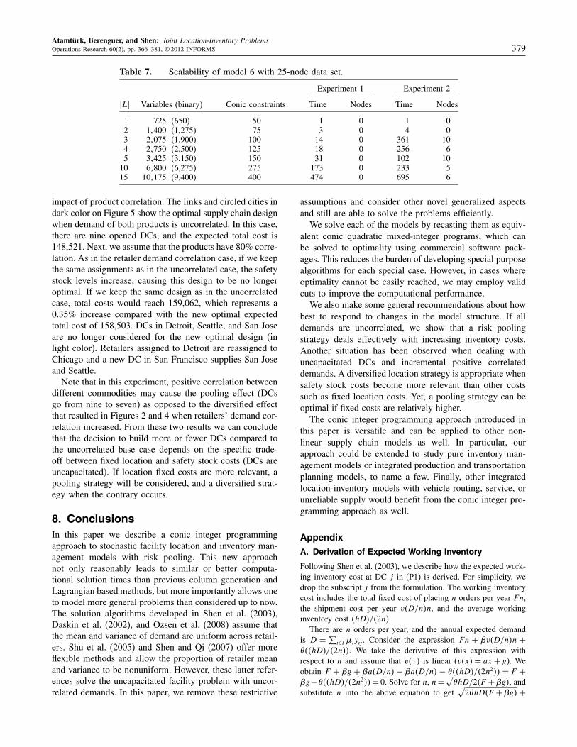
It is interesting to study the scalability of our most generalmodel. To do so, we increase the number of commodities(L) and observe the CPU times and the number of nodesexplored in the search tree in two different experiments.Experiment 1 assumes uncorrelated demand between dif-ferent retailers and different products and a fixed known


Table 5. Impact of correlation coefficient on solving (CQMIP3).

CPLEX CPLEX + Cuts

�ii′ Average cost Time % Rgap Nodes Time % Rgap Nodes Cuts

0 2111521 14 0010 7 14 0010 3 20.1 2131356 32 0032 17 24 0030 4 30.3 2151429 73 0076 153 89 0075 109 60.5 2231102 302 2051 710 262 1098 375 110.6 2281836 844 2047 31204 404 1037 11109 190.7 2291826 11156 4001 51219 674 2050 11354 21

Table 6. Impact of lead time variability.

�LjCost DCs Opened DCs Closed DCs

0 1011868 4 New York, Los Angeles, —Chicago, Houston

0.1 1251231 4 Philadelphia, Indiana New York,Chicago

0.2 1341529 5 New York, San Diego, Philadelphia,Baltimore Los Angeles

0.3 1411152 5 — —0.4 1471305 5 Philadelphia, New York,

San Antonio Houston0.5 1521090 6 Houston, San Francisco San Antonio

lead time of one at each DC (i.e. block matrices U andW are diagonal). Experiment 2 assumes nonzeros in all theelements of our block matrices. In particular, there is a cor-relation of 0.1 between different retailers, 0.1 between dif-ferent products, and a 0.1 standard deviation of all DCs’lead times. In each run we take the average of 10 randominstances based on some randomly generated parameters(refer to Table D.1).

As expected, we observe a better computational perfor-mance for experiment 1 compared to experiment 2, dueto sparsity of the correlation matrices and fixed lead time.Overall, we observe a good scalability as a function of �L�.

For the 88-node data set when �L� = 3 (or more), themodels become too large (18 million columns, 6 million

Figure 3. Cost as a function of retailers’ demand cor-relation and lead time variability.

0.50.4

0.30.2

0.101.0

0.870,000–77,000

50,000

40,000 0

Obj

ectiv

e va

lues

(co

sts)

70,000

60,000

40,000–50,000

60,000–70,00050,000–60,000

0.6

0.4

0.2

Correlation(retailers’ demand)

Lead timestandard

rows, and more than 6 million binary variables) to solve.Our computer runs out of 8 GB memory during model gen-eration with IBM ILOG Concert Technology. This suggeststhat for solutions of very large-scale models, column and/orrow generation methods would be needed.

Finally, we show an example of the impact of productcorrelation on the 25-node supply chain with two products.To isolate the correlation effect, we assume that lead timeis fixed, retailer demand is uncorrelated, and all DCs areuncapacitated. The latter assumption causes both productsto share the same DCs and assignments between DC andretailer. This way we are able to exclusively focus on the

Figure 4. Number of DCs as a function of retailers’demand correlation and lead time variability.

1.00

0.3

Lead timestandarddeviation0.90.80.70.60.50.40.30.20.10

Opt

imal

num

ber

of D

Cs

14

15

16

17

18

19

Correlation factor(retailers’ demand)

Figure 5. The effect of correlated product demand onthe supply chain.


Table 7. Scalability of model 6 with 25-node data set.

Experiment 1 Experiment 2

�L� Variables (binary) Conic constraints Time Nodes Time Nodes

1 725 (650) 50 1 0 1 02 11400 (1,275) 75 3 0 4 03 21075 (1,900) 100 14 0 361 104 21750 (2,500) 125 18 0 256 65 31425 (3,150) 150 31 0 102 10

10 61800 (6,275) 275 173 0 233 515 101175 (9,400) 400 474 0 695 6

impact of product correlation. The links and circled cities indark color on Figure 5 show the optimal supply chain designwhen demand of both products is uncorrelated. In this case,there are nine opened DCs, and the expected total cost is148,521. Next, we assume that the products have 80% corre-lation. As in the retailer demand correlation case, if we keepthe same assignments as in the uncorrelated case, the safetystock levels increase, causing this design to be no longeroptimal. If we keep the same design as in the uncorrelatedcase, total costs would reach 159,062, which represents a0.35% increase compared with the new optimal expectedtotal cost of 158,503. DCs in Detroit, Seattle, and San Joseare no longer considered for the new optimal design (inlight color). Retailers assigned to Detroit are reassigned toChicago and a new DC in San Francisco supplies San Joseand Seattle.

Note that in this experiment, positive correlation betweendifferent commodities may cause the pooling effect (DCsgo from nine to seven) as opposed to the diversified effectthat resulted in Figures 2 and 4 when retailers’ demand cor-relation increased. From these two results we can concludethat the decision to build more or fewer DCs compared tothe uncorrelated base case depends on the specific trade-off between fixed location and safety stock costs (DCs areuncapacitated). If location fixed costs are more relevant, apooling strategy will be considered, and a diversified strat-egy when the contrary occurs.

8. ConclusionsIn this paper we describe a conic integer programmingapproach to stochastic facility location and inventory man-agement models with risk pooling. This new approachnot only reasonably leads to similar or better computa-tional solution times than previous column generation andLagrangian based methods, but more importantly allows oneto model more general problems than considered up to now.The solution algorithms developed in Shen et al. (2003),Daskin et al. (2002), and Ozsen et al. (2008) assume thatthe mean and variance of demand are uniform across retail-ers. Shu et al. (2005) and Shen and Qi (2007) offer moreflexible methods and allow the proportion of retailer meanand variance to be nonuniform. However, these latter refer-ences solve the uncapacitated facility problem with uncor-related demands. In this paper, we remove these restrictive

assumptions and consider other novel generalized aspectsand still are able to solve the problems efficiently.

We solve each of the models by recasting them as equiv-alent conic quadratic mixed-integer programs, which canbe solved to optimality using commercial software pack-ages. This reduces the burden of developing special purposealgorithms for each special case. However, in cases whereoptimality cannot be easily reached, we may employ validcuts to improve the computational performance.

We also make some general recommendations about howbest to respond to changes in the model structure. If alldemands are uncorrelated, we show that a risk poolingstrategy deals effectively with increasing inventory costs.Another situation has been observed when dealing withuncapacitated DCs and incremental positive correlateddemands. A diversified location strategy is appropriate whensafety stock costs become more relevant than other costssuch as fixed location costs. Yet, a pooling strategy can beoptimal if fixed costs are relatively higher.

The conic integer programming approach introduced inthis paper is versatile and can be applied to other non-linear supply chain models as well. In particular, ourapproach could be extended to study pure inventory man-agement models or integrated production and transportationplanning models, to name a few. Finally, other integratedlocation-inventory models with vehicle routing, service, orunreliable supply would benefit from the conic integer pro-gramming approach as well.

Appendix

A. Derivation of Expected Working Inventory

Following Shen et al. (2003), we describe how the expected work-ing inventory cost at DC j in (P1) is derived. For simplicity, wedrop the subscript j from the formulation. The working inventorycost includes the total fixed cost of placing n orders per year Fn,the shipment cost per year v4D/n5n, and the average workinginventory cost 4hD5/42n5.

There are n orders per year, and the annual expected demandis D =

∑

i∈I �iyij . Consider the expression Fn + �v4D/n5n +

�44hD5/42n55. We take the derivative of this expression withrespect to n and assume that v4 · 5 is linear (v4x5 = ax + g). Weobtain F + �g + �a4D/n5 − �a4D/n5 − �44hD5/42n255 = F +

�g−�44hD5/42n255= 0. Solve for n, n=√

�hD/24F +�g5, andsubstitute n into the above equation to get

√

2�hD4F +�g5 +


�aD =√

2�h4F +�g5√

∑

i∈I �iyij + �a∑

i∈I �iyij . This expres-sion is part of the objective function in (P1).

B. Algorithm to Find Polymatroid Cuts

The following is the implementation of Edmond’s greedy algo-rithm (Edmonds 1970) for our separation problem. For each j ∈

J , do:1. Given y∗

j ∈ 60117�I � and t∗j , sort y∗ij in nonincreasing order

y∗

415j ¾ y∗

425j ¾ · · · 0

2. For i = 11 0 0 0 1 �I �, let Si = 84151 4251 0 0 0 1 4i59 and �4i5 =√

∑

k∈Si�24k5 −

√

∑

k∈Si−1�24k5.

3. If �j = �y∗j > t∗j , we add the extended polymatroid cut

�yj ¶ tj to the formulation.

C. Heuristic to Find Cover Cuts

The following is the implementation of Atamtürk and Narayanan’scover inequality separation algorithm (Atamtürk and Narayanan2009) for our problem. Let yij = 1 − y∗

ij for i ∈ I1 j ∈ J . For eachj ∈ J and for each distinct pair i1 and i2 in I do:

1. Solve the following system of equations on variables �

and �:

yi1j = Lj�i1�+ z2

�Lj�2i1�1

yi2j = Lj�i2�+ z2

�Lj�2i2�0

2. If 4�1�5 ¾ 0, then sort each i in nondecreasing order ofyij/4Lj�i1

�+ z2�Lj�

2i �5; that is,

y415j

Lj�415�+ z2�Lj�

2415�

¶y425j

Lj�425�+ z2�Lj�

2425�

¶ · · · 0

3. Assign z4i5 = 1 following the established order until

z�√

Lj

√

∑

i∈I �2i zij +Lj

∑

i∈I �izij >Cj .4. If � = yz < 1, then we add the cover cut

∑

i∈S xi ¶ �S� − 1to the formulation, where S is the ground set for z.

D. Parameter Values

Table D.1. Parameters used in all experiments.

Parameter Value

Used in all experimentsdij Great circle distanceFj , gj 10aj 5h, �, Lj 1� 0.975z� 1.96

Table 1 (881150 nodes)fj From Daskin (1995) divided by

100, if 88 nodes 100, if 150nodes

�i, �2i Demand 1 from Daskin (1995)

divided by 1,000, �i

Table D.1. Continued

Table 3 (151881150 nodes)fj From Daskin (1995) divided by

100, if 15 or 88 nodes 100,000,if 150 nodes

�i, �2i Description in Özsen et al.

(2008), �i

4�1�5 (0000001100001)

Table 4 (88 nodes)fj Uniform [4010001501000]�i, �

2i Description in Özsen et al. (2008)

41 + �i5, �j41 + �i54�1�5 (000004110)

Figure 1 (25 nodes)fj 10,000�i, �i Demand 1 from Daskin (1995),

demand 2 from Daskin (1995)4�1�51Cj (0000001100001), 17,000,000

Figures 2, 3, 4 (25 nodes)fj 1,000�i, �i Demand 1 from Daskin (1995),


Table 5 (25 nodes)fj Uniform [4010001501000]�i, �i Demand 1 from Daskin (1995)

41 + �i5, demand 2 from Daskin(1995) 41 + �i5

4�1�51Cj (00000011000001), 17,500,000

Table 6 (25 nodes)fj 10,000�i,�i Demand 1 from Daskin (1995),


Table 7 (25 nodes)fj Uniform [4010001501000]�il, �il Demand 1 from Daskin (1995)

41 + �il5, demand 2 from Daskin(1995) 41 + �il5

4�1�51Cj (00001100001), 2,000,000,000

Figure 5 (25 nodes)fj 6,000�i11�

2i1 Demand 1 from Daskin (1995)

divided by 100, �i1�i21�

2i2 Demand 2 from Daskin (1995)

divided by 100, �i24�1�51Cj (000011001), 2,000,000,000

Acknowledgments

The authors thank Lian Qi and Leyla Özsen for sharing theircomputer programs with the authors. They are also grateful to theanonymous referees and the associate editor for their insightfulcomments. This research was partially supported by the NationalScience Foundation [Grant CMMI 1068862].

ReferencesAlizadeh, F., D. Goldfarb. 2003. Second-order cone programming. Math.

Programming 95(1) 3–51.


Atamtürk, A., V. Narayanan. 2008. Polymatroids and mean-risk minimiza-tion in discrete optimization. Oper. Res. Lett. 36(5) 618–622.

Atamtürk, A., V. Narayanan. 2009. The submodular knapsack polytope.Discrete Optim. 6(4) 333–344.

Atamtürk, A., V. Narayanan. 2010. Conic mixed-integer rounding cuts.Math. Programming 122(1) 1–20.

Atamtürk, A., V. Narayanan. 2011. Lifting for conic mixed-integer pro-gramming. Math. Programming 126(2) 351–363.

Ben-Tal, A., A. S. Nemirovski. 2001. Lectures on Modern Convex Opti-mization: Analysis, Algorithms, and Engineering Applications, Vol. 2.Society for Industrial and Applied Mathematics, Philadelphia, PA.

Çezik, M. T., G. Iyengar. 2005. Cuts for mixed 0-1 conic programming.Math. Programming 104(1) 179–202.

Charnes, J. M., H. Marmorstein, W. Zinn. 1995. Safety stock determina-tion with serially correlated demand in a periodic-review inventorysystem. J. Oper. Res. Soc. 46(8) 1006–1013.

Dasci, A., V. Verter. 2001. The plant location and technology acquisitionproblem. IIE Trans. 33(11) 963–974.

Daskin, M. S. 1995. Network and Discrete Location: Models, Algorithmsand Applications. Wiley, New York.

Daskin, M. S., C. R. Coullard, Z. J. M. Shen. 2002. An inventory-locationmodel: Formulation, solution algorithm and computational results.Ann. Oper. Res. 110(1) 83–106.

Edmonds, J. 1970. Submodular functions, matroids, and certain polyhedra.Combin. Structures and Their Appl. 11 69–87.

Erkip, N., W. H. Hausman, S. Nahmias. 1990. Optimal centralizedordering policies in multi-echelon inventory systems with correlateddemands. Management Sci. 36(3) 381–392.

Fine, C. H., R. M. Freund. 1990. Optimal investment in product-flexiblemanufacturing capacity. Management Sci. 36(4) 449–466.

Geoffrion, A. M., G. W. Graves. 1974. Multicommodity distributionsystem design by Benders decomposition. Management Sci. 20(5)822–844.

Goyal, M., S. Netessine. 2011. Volume flexibility, product flexibility orboth: The role of demand correlation and product substitution. Man-ufacturing Service Oper. Management 13(2) 180–193.

Inderfurth, K. 1991. Safety stock optimization in multi-stage inventorysystems. Internat. J. Production Econom. 24(1–2) 103–113.

Johnson, G. D., H. E. Thompson. 1975. Optimality of myopic inventorypolicies for certain dependent demand processes. Management Sci.21(11) 1303–1307.

Kuo, Y. J., H. D. Mittelmann. 2004. Interior point methods for second-order cone programming and OR applications. Comput. Optim. Appl.28(3) 255–285.

Nahmias, S. 1993. Production and Operations Analysis. Irwin ProfessionalPublishing, Homewood, IL.

Özsen, L., C. R. Coullard, M. S. Daskin. 2008. Capacitated ware-house location model with risk pooling. Naval Res. Logist. 55(4)295–312.

Shen, Z. J. M. 2005. A multi-commodity supply chain design problem.IIE Trans. 37(8) 753–762.

Shen, Z. J. M. 2007. Integrated stochastic supply chain design models.Comput. Sci. Engrg. 9(2) 50–59.

Shen, Z. J. M., M. S. Daskin. 2005. Trade-offs between customer serviceand cost in integrated supply chain design. Manufacturing ServiceOper. Management 7(3) 188–207.

Shen, Z. J. M., L. Qi. 2007. Incorporating inventory and routing costs instrategic location models. Eur. J. Oper. Res.179(2) 372–389.

Shen, Z. J. M., C. Coullard, M. S. Daskin. 2003. A joint location-inventorymodel. Transportation Sci. 37(1) 40–55.

Shu, J., C. P. Teo, Z. J. M. Shen. 2005. Stochastic transportation-inventorynetwork design problem. Oper. Res. 53(1) 48–60.

Snyder, L. V., M. S. Daskin, C. P. Teo. 2007. The stochastic locationmodel with risk pooling. Eur. J. Oper. Res. 179(3) 1221–1238.

Qi, L., Z. J. M. Shen. 2007. A supply chain design model with unreliablesupply. Naval Res. Logist. 54(8) 829–844.

A Conic Integer Programming Approach to Stochastic Joint … · 2018-08-16 · mixed-integer...

Documents

Transcript of A Conic Integer Programming Approach to Stochastic Joint … · 2018-08-16 · mixed-integer...