4

A Comprehensive Analysis of MALDI-TOF Spectrometry Data

Malgorzata Plechawska-Wojcik Lublin University of Technology,

Poland

1. Introduction

Today, biology and medicine need developed technologies and bioinformatics methods. Effective methods of analysis combine different technologies and can operate on many levels. Multi-step analysis needs to be performed to get information helpful in diagnosis or medical treatment tasks. All those processing needs the informatics approach to bioinformatics, proteomics and knowledge discovery methods.

Scientists find proteomic data difficult to analyse. On the other hand, the proteomic analysis of tissues like blood, plasma and urine might have an invaluable contribution to biological and medical research. They seem to be an alternative way of searching for new diagnostic methods, medical treatment and drug development. For example, typical analytical methods have problems with dealing with cancer diseases. Proteomics is a promising approach to those issues.

Proteomic signals carry an enormous amount of data. They reflect whole sequences of proteins responsible for various life processes of the organism. This diversity of data makes it hard to find specific information about, for example, the severity of the cancer. To discover interesting knowledge researchers need to combine a variety of techniques. One of the basic methods of tissue analysis is mass spectrometry. This technique measures the mass-to-charge ratio of charged particles.

There are various types of mass spectrometry techniques. They differ in the types of ion source and mass analysers. The MALDI-TOF (Coombes et al., 2007) is a technique widely applicable in proteomic research. The MALDI (Matrix - Assisted Laser Desorption / Ionisation) is a soft ionisation technique and the TOF (time of flight) is a detector determining the mass of ions. Samples are mixed with a highly absorbent matrix and bombarded with a laser. The matrix stimulates the process of transforming laser energy into excitation energy (Morris et al., 2005). After this process analyte molecules are sputtered and spared. The mass of ions is determined on the basis of time particular ions take to drift through the spectrometer. Velocities and intensities of ions obtained in such a way (Morris et. al., 2005) are proportional to the mass-to-charge (m/z) ratio.

The analysis of mass spectrometry data is a complex task (Plechawska 2008a; Plechawska 2008b). The process of gaining biological information and knowledge from raw data is composed of several steps. A proper mass spectrometry data analysis requires creating and

www.intechopen.com

Medical Informatics

70

solving a model and estimating its parameters (Plechawska 2008a). There are many types of models and methods which might be used. All of them, however, include mass spectrum preprocessing, which need to to be done before the general analysis. Preprocessing methods need be adjusted to data. Spectra have some noise levels which need to be removed. Denoising and baseline corrections are done to get rid of the noise which might be caused by spectrometer inaccuracy or by sample contamination. Also, normalisation should be performed. After these steps, peak detection and quantification can be done. Successful preprocessing is a condition of reliable mass spectrometry data analysis (Coombes et. al., 2007). All elements of the mass spectral analysis are closely related. Any performed operation has an influence on the further quality of results. Not only the set of methods and parameters is important. The proper order of methods also matters.

There is an extensive literature on mass spectrum analysis problems (Plechawska et al., 2011). One can find several techniques of peak detection and identification. A very popular approach is to use local maxima and minima. Such methods (Morris et. al., 2005; Yasui et. al., 2003; Tibshirani et. al., 2004) usually compare local maxima with noise level. There are also methods (Zhang et al., 2007) considering the signal to noise ratio. This ratio needs to be high enough to identify a true peak with a local maximum. Such methods choose peaks with the highest intensities. Similar ideas (Mantini et al., 2007; Mantini et al., 2008) consider using predefined thresholds depending on the noise level. Peak detection is usually done on denoised spectra. Moreover, intervals based on local maxima and minima are calculated. Constituent intervals have differences between the height of the maxima and minima found. In addition, using the mean spectrum was proposed (Coombes et. al., 2007). Other methods (Fung & Enderwick, 2002) use regions which are determined to enable easier peak detection based on the signal to noise ratio. Peaks need to have an large enough area and appropriate width, which depends on starting and ending points of peaks and valleys on both sides of the apex. Peaks may be also considered a continuous range of points where intensities are high enough (Eidhammer et al., 2007). Another approach is using peak clusters to find peaks of the highest intensities (Zhang et al., 2007). There are also methods which try to distinguish true peaks from noise and contaminants. Du et al. (Du et al., 2006) for example use the shape of peaks. Some methods consider the mass spectrometer resolution. There are also methods turning spectrum decomposition into the sum of their constituent functions (Randolph et al., 2005) or the sum of the Levy processes (Zhang et al., 2007).

2. Mass spectrum modelling

Before the main decomposition, preprocessing needs to be performed. In our analysis we apply the following methods:

Trimming is the cutting of the lower and/or upper parts of spectra according to specified boundaries designated by the type of analysis. Binning with a defined mask is a technique reducing the number of data points in a single spectrum. The researcher has to keep in mind that this process additionally gives noise reduction. This is optional method. It should be used if the number of the spectrum data points is too large to perform efficient calculations. Interpolation is a process which may be defined as the unification of measurements points along the m/z axes. It is needed in the case of dealing with a data set of spectra. Unification is obligatory if all spectra are to be analysed simultaneously.

www.intechopen.com

A Comprehensive Analysis of MALDI-TOF Spectrometry Data

71

Baseline correction is an essential part of preprocessing. Baseline is a special type of noise which needs to be removed. It represents a systematic artifact formed by a cloud of matrix molecules hitting the detector (Morris et al., 2005). This noise is seen in the early part of the spectrum. Among typical methods of baseline correction one can find a simple frame with fixed sizes and quantilles. Our experience shows that a simple frame with the appropriate size is good enough.

Smoothing and noise reduction might be performed in several ways. One can use

wavelet transformation (for example the widely-used undecimated discrete-wavelet

transformation, UDWT), the least-squares digital polynomial filter (Savitzky and Golay

filters) or nonparametric smoothing (locally-weighted linear regression with specified

window size and type of kernel). In our analysis we usually make use of a polynomial

filter. However it is also possible to skip noise reduction due to the specificity of the

decomposition method.

Normalisation is an important preprocessing method consisting in minimising

differences between spectra and thier peak intensities. The most popular methods are

scaling all spectra to total ion current (TIC) value or to constant noise. We found the TIC

value appropriate for our analysis. It is calculated as the area under the curve, usually

using the trapezoidal method.

The mean spectrum calculation is useful in analysing data sets containing many mass

spectra of the same type. The mean spectrum facilitating the simultaneous analysis of

all spectra. Even small peaks are usually detected during mean spectrum analysis.

Finding peaks in the mean spectrum are regarded as even more sensitive (Morris et al.,

2005).

Most preprocessing steps need to be conducted under the supervision of the user. The

parameters of the baseline correction especially need to be adjusted to the data. The order of

operations is fixed. Many research studies were conducted in this area and this order has

become a standard over the past few years. Some of operations might be skipped - but it

should be depended on the data.

2.1 Gaussian mixture model decomposition

Our method of spectrum analysis is based on Gaussian Mixture decomposition. The

Gaussian Mixture Model (GMM) (Everitt & Hand, 1981) with the appropriate number of

components is suitable for spectrum modelling because they also might be used for noise

modelling and determining. The idea of using GMM is that one peak is represented by a

single distribution (Plechawska-Wojcik, 2011a). All peaks and the noise are represented by

the mixture model. A mixture model is a combination of a finite number of distributions.

The number of components might be estimated by the Bayesian Information Criterion (BIC).

The fitting is done with the Expectation-Maximisation algorithm (EM) performing maximising the likelihood function. A typical mixture model is a combination of a finite number of probability distributions (eq. 1).

( , ,..., , ,..., ) ( , )1 11

Kmixf x p p f x pK K k k kk

(1)

www.intechopen.com

Medical Informatics

72

where K is the number of components in the mixture and , 1,2,...k Kk are weights of the

particular component, 11

K

kk

. The Gaussian distribution is given with two parameters:

mean k and standard deviation k .

The Expectation-Maximisation (EM) algorithm (Dempster et al., 1977) is a nonlinear method and is composed of two main steps performed in a loop. The expectation step (E) consists of the calculation of the distribution of hidden variables (eq. 2).

( , )

( | , )( , )1

old oldf x pold k k np k x pn old oldK f x pk k n

(2)

The maximisation step (M) calculates new mixture parameter values. Formulas adjusted to mass spectrometry data are given by (eq. 3).

( | , )1 , 1,2,...,( | , )1

2( ) ( | , )2 1( ) , 1,2,...,( | , )1

( | , )1

N x y p k x pnew n n n n old k Kk N p k x p yn n old nnewN x p k x pnew n n k n old k Kk N p k x p yn n old n

oldN p k x p ynew n n nk N

(3)

The calculated means represent the M/Z values of peaks, whereas standard deviations indicate the widths of peaks. Weights determine the shares of particular peaks in the spectrum. This method may be applied to individual spectra or to the mean spectrum calculated from the data set. In the case of the mean spectrum, the obtained means and standard deviations are treated as, respectively, M/Z values and widths of peaks in every single spectrum of the data set. The weights are calculated separately for each spectrum. The simple least-squares method might be used to obtain those weights.

Examples of a mass spectra collection analysis are presented in Fig.1. Fig.1a,c present the

results of our calculations for single spectra with 40 components and Fig.1b,d presents the

results with the use of the mean spectrum. The mean spectrum is presented in Fig.2.

2.2 Parameters of the decomposition process

There are several aspects which need to be considered before the decomposition. The first is the number of components which needs to be known before carrying out the analysis. The best solution is to use one of the available criteria. These are BIC (the Bayesian Information Criterion), AIC (the Akaike Information Criterion), ICOMP (the Information Complexity Criterion), AWE (the Approximate Weight of Evidence), MIR (the Minimum Information Ratio) and NEC (the Normalised Entropy Criterion). The proper number of components should minimise (or for some criteria maximise) the value of the chosen criterion. Most of

www.intechopen.com

A Comprehensive Analysis of MALDI-TOF Spectrometry Data

73

Fig. 1. A comparison of results obtained with and without the mean spectrum.

Fig. 2. The mean spectrum.

www.intechopen.com

Medical Informatics

74

the mentioned criteria are based on the likelihood function. We chose the BIC criterion

because it is easy to calculate and it considers such parameters as the size of the sample and

the value of the likelihood function. Formulas defining the mentioned criteria are presented

in Tab1. In the presented formulas models the parameters are marked as .

The main disadvantage of using criteria to estimate the number of components is the fact

that it is a time-consuming method. A single use of each criterion gives a result for the single

number of components. To obtain reliable results the calculations need to be repeated many

times for each single number of components. The example of using the BIC criterion for data

presented in Fig.1 and Fig.2 is shown in Fig.3. According to Fig.3, the BIC criterion needs to

be maximised. Results stabilise for 40 components, so this number was considered to be

appropriate for the further analysis.

There are also different ways of dealing with the unknown number of the components

problem. It is possible to use different, simple method of peak detection. Such methods

work fast, because they are based on local maxima and minima. However, it is a reliable

method only in the case of spectra which do not have many overlapped peaks.

Criterions Formulas

BIC (the Bayesian

Information Criterion)

(Schwarz, 1978)

ˆ( ) 2 log ( ) logBIC g L d n

AIC (the Akaike

Information Criterion)

(Akaike, 1974)

ˆ( ) 2 log ( ) 2AIC g L d

ICOMP (the Information

Complexity Criterion)

(Bozdogan, 1993;

Bozdogan, 1990)

ˆ( ) 2 log ( ) 1 2

1 11 1 2 2ˆ ˆ ˆ ˆ ˆlog[ { ( ) ( ) ( ) }]1 2 21 1

ˆ ˆ( 2) log(| | log( ) log(2 )21 1

1( 1)

2

ICOMP g L C C

g PC d d tr tr tri i i i i vv

i vg P

C p p n gp ni ii v

d gp gp p

AWE (the Approximate

Weight of Evidence)

(Banfield & Raftery, 1993)

( ) 2 log 2 (3 /2 log )AWE g L d nC

MIR (the Minimum

Information Ratio)

(Windham & Cutler,

1993)

1 1( ) 1 /m m m mMIR g

NEC (the Normalized

Entropy Criterion)

(Celeux & Soromenho,

1996)

ˆ( )( )

ˆ ˆlog ( ) log ( *)

EN rNEC g

L L

Table 1. Criteria used to estimate the number of components.

www.intechopen.com

A Comprehensive Analysis of MALDI-TOF Spectrometry Data

75

Fig. 3. The estimation of the number of components using BIC criterion.

It is also possible to reduce the number of components during calculations. This correction is

based on the values of probabilities calculated during the M step of the EM procedure. If

they are too small (very close to 0) it usually means that the number of components is

overstated. Essential support is also given by the model testing procedure. EM calculations

might be suspended after a few iterations. The researcher can check the so-far obtained

weights and means indicating the peak localisations. If he/she finds many very small

weights, or means are found to be located very close to each other, it usually means that the

number of specified components is too large. Suspending the EM procedure makes sense

because of the characteristic of the algorithm. It converges very fast at the beginning and

after that it slows down. That is why the checking of the results after 10-20 calculations fairy

well illustrates the quality of the modelling.

The other aspect which needs to be considered is the generation of initial parameters values.

The EM algorithm is sensitive to the initial values. If they are poorly chosen, the quality of

calculations might not be reliable. One option is to randomise them from the appropriate

distribution. The better one, however, is to use the simple method of peak detection. This

method gives less biased, more reliable results. The important thing is to add small

Gaussian arousals to the results obtained from the peak-detection method.

The next decomposition aspect to be mentioned is the stop criterion. According our

simulations one good idea is to use a stop criterion based on the likelihood value (eq. 4) and

the maximum likelihood rule (eq. 5). The maximum likelihood rule states that the higher

value of the likelihood function, the better the parameters estimation can be gained. Using

the maximum likelihood rule gives the certainty of stability because of monotonicity of the

likelihood function (Fig. 4).

www.intechopen.com

Medical Informatics

76

Fig. 4. The monotinicity of the likelihood rule.

( , ) ( ) ( , ,..., , ) ( , )1 21

NL p x L p f x x x p f x pN n

n (4)

arg max ( , )1

Np f x pn

n

(5)

Maximum likelihood itself is an efficient method of parameters estimation. However, it

cannot be used in the problem of spectral decomposition. The problem consists in the fact

that we do not know the assignment of the Gaussians to the respective peaks. The EM

algorithm deals with it using hidden variables. The probabilities of assignment are

calculated in each iteration and finally the right assignment is found.

The decomposition with the EM algorithm is slower than using simple methods based on

local minima and maxima. However, it copes better with spectra containing overlapped

peaks. There are many examples of spectra which cannot be solved by such typical methods.

Examples of decomposed spectra obtained from different methods are presented in Fig. 5.

The next argument for Gaussian decomposition is that using an EM algorithm and a mean spectrum eliminates the necessity for alignment procedure processing. This operation is done to align detected peaks among all spectra in the dataset. Those mismatches are due to measurement errors. The alignment procedure needs to be performed on most of peak processing procedures. It is a hard and difficult process. EM decomposition is based on the assumption that peaks are covered with Gaussians defined by means and standard deviations. That is why the m/z values do not need to match exactly to Gaussians means – we accept slight differences between peaks among different spectra in the dataset.

The method discussed in this chapter is based on Gaussian distributions. However, it is also possible to use different distributions, like Poisson, log-normal or beta. High-resolution spectra contain asymmetric peaks with the right skewedness. In such cases it is a good idea to use log-normal or beta distributions (Guindani et al., 2006). MALDI-ToF spectra are low-resolution and there is no skewedness seen. That is why Gaussian distributions are more appropriate to use. The second reason we use Gaussian distributions is connected with the error of the spectrometer measurement. This noise can be modelled in a natural way with Gaussians.

www.intechopen.com

A Comprehensive Analysis of MALDI-TOF Spectrometry Data

77

Fig. 5. Results of spectra decomposed with various methods and tools: a) the Cromwell package b) the PrepMS tool c) the MassSpec Wavelet tool d) the PROcess package e) the mspeaks function (Matlab).

Single peaks are, in fact, modelled with single Gaussians. The appropriate choice of

distribution parameters allows the representation of peak shapes and measurement errors. It

is also easy to write the model. It is worth paying attention to the fact that single Gaussians

might be used only in the case of perfectly-separated peaks. In practice, the analysis of the

real spectra is done using mixtures of Gaussian distributions. Using a mixture of Gaussian

distributions instead of single Gaussian distributions additionally takes account of

interactions between closely-located peaks. Mass spectra reflect a number of processes

occurring in an organism. Those processes are usually correlated with each other. They have

their representation in the characterising spectra, especially in the lack of separability among

its particular peaks. This fact needs to be considered during the analysis. The application of

mixture models allows the considering of dependences between spectral peaks. It also

facilitates the modelling of overlapped measuring errors placed in adjacent regions of the

spectrum. Separate-peak identification could be a case of the incorrect assessment of the

individual Gaussians variances, because it is not possible to completely separate them.

Mixture modelling makes it possible to detect all peaks simultaneously and correct

measurement inaccuracies. However, mixture model parameter solving is a complicated

task that needs the determination of many properties like the number of components, the

type of stop criterion or calculation accuracy.

3. Data classification

Preprocessing steps and decomposition are the first steps in the analysis. The second is

classification, which might be used in the process of significant peak determination.

Classification allows the search for the distinction between ill and healthy patients. It is also

www.intechopen.com

Medical Informatics

78

possible to look for the stage of disease progression or to check reactions (positive or

negative) to medical treatment.

Classification of mass spectra collection is an essential but also difficult task, because of the specificity of the data. The most common classification tasks are based on the supervised learning. It usually consists of categorising data into two groups (for example ill and healthy). There are also attempts to classify data into three or more groups. Such classification tasks are, however, more complicated and they are not included in this chapter.

Classified objects are usually represented by vectors of observed, measured or calculated

features. Supervised learning classification assumes that the unknown function is to be

assigned to each object of population O as a label of one class. The classification process is

based on the learning set U which is a subset of the whole data set O. Each element io of the

learning set is composed of the object representation and a class label. This object

representation is an observation vector of the features. The whole set is divided into c

separated subsets and one-subset observations are numbered among one of the c classes.

Such supervised learning is widely used in biomedical applications.

3.1 Classifiers construction

The construction of classifiers is based on several rules. Multiple different classifiers might be constructed on the basis of one single learning set. The ideal situation would be to choose the proper classifier on the basis of the number of misclassifications of the new, random observation. However, in reality bad classification probabilities are unknown. They might be estimated from a validation probe, which is a random sample, independent of the learning probe, where objects’ belonging to classes are unknown. The misclassification probability of a specific classifier is estimated with mistakes done by the classifier on the validation probe. Classifier evaluation should be done using observations independent of those from the learning probe. In other cases the classifier will be biased.

The ultimate classifier evaluation is done with a test probe. It needs to be independent of other probes and it needs to have information about objects’ membership of classes. If only one classifier is to be tested or basis size of the set is small, the validation probe might be omitted. In practice, the usually-chosen proportion is the division into 50% on the learning probe and 25% each for the validation and test probes (Cwik & Koronacki, 2008). However, in practice, the division depends on the specificity of the data set.

The classifier makes the decision about the belonging to classes on the basis of the learning probe. However, the trained classifier will need to operate on large datasets. These datasets are larger than sets used for classifier training. It makes non-zero the probability of a wrong decision (Stapor, 2005). The classifier is used for data other than those for which it was constructed. That is why the classifier quality depends on its generalisation ability. In practice it means that the learning properties need to be representative of all the population. On the other hand, nonessential properties should be omitted, because they only constitute features of the specific learning set.

The most popular measures of classification quality are classification accuracy (a proportion of correctly-classified sets) and error rate (a proportion of misclassified sets). Important rates are also TP (True Positives) – the number of correctly-classified positive sets, TN (True

www.intechopen.com

A Comprehensive Analysis of MALDI-TOF Spectrometry Data

79

Negatives) – the number of correctly-classified negative sets, FP (False Positives) – the number of incorrectly-classified positive sets, FN (False Negatives) – the number of incorrectly-classified negative sets.

Among useful measures one can also find sensitivity and specificity. This sensitivity is

defined as a proportion of truly positive and false negative results (eq. 6). It is interpreted as

ability of a classifier to identify the phenomenon if it really exists.

TP

sensitivityFN TP

(6)

On the other hand the specificity is a proportion of truly negative results and the sum of

truly negative and truly positive results (eq. 7). The specificity is interpreted as the ability to

reject truly false results.

TN

specificityTN FP

(7)

Sensitivity and specificity are opposed values – an increase in the one causes a decrease in the other.

The significant tool characterising a classifier’s features is the receiver-operating-

characteristic curve – known as the ROC curve. It is a chart of dependency between values:

1-specificity and sensitivity. Such a curve is created for a specific structure of the classifier

(specified type, parameters, number of input features). The total error of the classifier

remains unchanged. However, its division into values FP and FN is changed, because the

ROC curve examines the proportion between FP and FN. In the case of the random division

of objects, the ROC curve takes the shape of a curve going from the bottom left to the upper

right corner. The better the classification results are, the more concave the curve is. The ideal

situation will make the ROC curve go through the upper left corner of the chart.

An important factor in the classifier’s quality is the curve under the ROC curve, the so-called

AUC. The closer to the value 1 AUC is, the better are the classification results. An example

of ROC is presented in Fig 6.

3.2 Dealing with high dimensionality

Mass spectrometry data are characterised by high dimensionality. The number of

observations is significantly lower than the number of features. Each patient has a few

thousand data points or even more, whereas a typical dataset contains dozens or hundreds

of spectra. Typical classification and data mining techniques are designed to handle low-

dimensional data, such as sales or economic indicators. Low-dimensional datasets contain

many observations and just only a few, usually uncorrelated, features. Such data might be

analysed using any type of method, including graphical interpretation and unsupervised

learning. Dealing with high-dimensional data is much more difficult. The main problem is

the correlation of features which always occur in high-dimensional data. In fact, to obtain

statistical significance the number of observations should grow exponentially with the

dimensionality. The existence of dependent features prevents or hinders the classification

www.intechopen.com

Medical Informatics

80

Fig. 6. Example of the ROC curve.

using typical, widely-known methods. Moreover, a large number of correlated features has

a bad influence on the quality of the classification. This makes analysis difficult and

diversification is hard to obtain (Stapor, 2005). A large number of features causes also large

number of classifier parameters. It increases its complexity and susceptibility to over-

learning and decreases its flexibility. The existence of the curse of dimensionality (Mao et al.,

2000) proves that the complexity of the classifier has an impact on the classification quality.

The more complex the classifier is, the higher should be the proportion between the number

of observations and the number of features (Stapor, 2005). That is why high-dimensional

data must be properly processed, including the application of dimension-reduction

techniques. This task determines the success of the classification because of specificity of

mass spectral data.

Another problem of dealing with bio-medical data is signal strength. A typical signal of

mass spectrometry data carries information concerning the functions of the whole organism.

Moreover, the development of medical, diagnostic and prevention programmes gives

results for significantly less patients diagnosed with late-stage diseases. For example, cancer

diseases are usually diagnosed at the first or second clinical level. Such signals are difficult

to identify and to extract among the many different signals of the organism. Blood, serum or

urine contain proteins responsible for the range of typical, vital functions of the body. One

needs to notice that those proteins are much stronger than the signals of diseases.

One of the most frequently-used classifiers for mass spectrometry data is the Support

Vectors Machines (SVM) proposed by V.N. Vapnik (Vapnik et al., 1992; Vapnik, 1995;

Vapnik, 1998). The idea of this method is a classification using an appropriately-designated

discriminant hyperplane. Searching for such a hyperplane is performed by the Mercer

theorem and the optimisation of the quadratic objective function, with linear restrictions.

The SVM idea is based on searching for two parallel hyperplanes. If classification groups are

www.intechopen.com

A Comprehensive Analysis of MALDI-TOF Spectrometry Data

81

linearly separated, those hyperplanes should delimit the widest possible area which contain

no elements of the probe. The hyperplanes need to be based on so-called support vectors. If

learning sub-sets are not linearly separated, a penalty is introduced. The best separation

result is obtained for a higher dimensional space.

The SVM rule is presented in Eq. 8.

0 0( ) sgn( ( ) )sup. .

f x y x x bi iivect

(8)

where are Lagrange’s coefficients and b is a constant value. For inseparable classes the

additional restrictions take the form of Eq. 9.

1 , 1

1 , 1

x w b yi i ix w b yi i i

(9)

where i is a constant value 0i

Classifiers used in bioinformatics applications are solved with use of kernel functions. Such

a construction enables one to obtain non-linear shapes of discriminant hyperplanes. One of

the most popular kernel functions is the radial kernel (Eq. 10).

0 0( ) sgn( ( ) )sup. .

f x y K x x bi i ivect

(10)

Before the main classification of mass spectrometry data, dimension reduction needs to be

performed. Input data-sets for classification usually contain several hundreds or even

thousands of features. From the statistical point of view, using such a number of features is

unreasonable. Reduction might be carried out in two-stages. The first is spectrum

decomposition, which reduces dimensionality from thousands of features to hundreds. The

second step is applying feature reduction or selection techniques.

The first step in dimension reduction is based on applying the decomposition results. These results are used as a Gaussian mask, which is put on every single spectrum of the data set. This gives new values consisting of all spectra. Dimensions of mass spectrometry data decrease to the value of the GMM components number. The resultant matrix obtained after

these steps is n k , where n denoted the number of spectra and k the number of

components. The resultant matrix was the input data to the further dimension reduction and classification.

There are many reduction and selection techniques available. They attempt to find the

smallest data sub-set chosen with defined criteria among the whole data set. Too large a

number of features has an adverse impact on the classification results. A large number of

features causes an increase in computational complexity and lengthen calculation time.

There are two types of dimension reduction methods:

feature extraction – data are subjected to certain transformation – a new data set is obtained

www.intechopen.com

Medical Informatics

82

feature selection – a subset of the most optimal data is chosen.

One of commonly-known features extraction methods is the Partial Least Squares (PLS)

method (Barnhill et al., 2002). The method also facilitates classification. Feature selection in

the PLS method is performed with use of both X and Y data, so it considers the whole

structure of the learning set. The idea of the PLS method is to find latent vectors. Using

latent vectors allows simultaneous analysis and the decomposition of X and Y, including a

covariance between X and Y. Such an approach makes PLS a special case of Principal

Component Analysis (PCA) (Mao et al., 2000). The original version of PLS is a regression

method dealing with continuous values. Classification of mass spectrometry data usually

consists of assigning data to one of two groups. So, the matrix of dependent features (Y) is

composed of only two values. It is possible to directly apply PLS to mass spectrometry or

microarray data. However, it is better to use one of the few PLS modifications dedicated to

binary classification. The original PLS classification components are a linear combination of

predictor variables. Weights, however, are a nonlinear combination of predictor and

response variables (Nguyen & Rockeb, 2004). There are approaches (Liu & Rayens, 2007;

Boulesteix & Strimmer, 2006; Fort & Lambert-Lacroix, 2005; Nguyen & Rockeb, 2004; Man et

al., 2004; Huang et al., 2005) applying the original PLS to categorical, binary responses.

However, research confirms that it is better to use PLS procedures adjusted to binary

responses (Nguyen & Rockeb, 2002). One can use a hybrid-PLS method based on singular-

value decomposition. Another approach is the hybrid-PLS method based on logistic

regression predictors, where the PLS components are calculated as weighted averages of the

original predictor/explanatory variables. Also, weights are dependent on sample predictor

variances and the partial correlation coefficient (Garthwaite, 1994; Nguyen & Rockeb, 2004).

PLS is also used in conjunction with Linear Discriminant Analysis (LDA) (Boulesteix &

Strimmer, 2006; Boulesteix, 2004; Liu & Rayens, 2007). Fort and Lambert-Lacroix (Fort &

Lambert-Lacroix, 2005) proposed a combination of the PLS and Ridge penalty.

Among the most popular features selection method one can find the SVM-RFE and

traditional T test. The SVM-RFE (Support Vector Machine Recursive Feature Elimination)

(Wold, 1996) method is a features-selection method. Features selection is performed with the

propagation-backward method. The procedure starts with a full range of input features and

features are successively removed. Only one feature is removed at a time. As a range

criterion SVM weights coefficients are used. Therefore the SVM-RFE method is closely

related to the SVM classification. The T test is a very common technique of feature selection.

The most significant features are chosen according the T test. For each feature a T-test range

is calculated. This statistics treat all features as independent and this assumption is usually

not met. However, the T test is successfully used for protein data classification.

3.3 Learning the classifier

After applying dimension reduction, supervised classification is preformed with the SVM method. Our results (Plechawska-Wójcik, 2011) show that the best results can be obtained using linear SVM and SVM with the Gaussian Radial Basis Function kernel. However, before the learning process, proper classification parameters need to be estimated. Such an estimation is usually performed experimentally, for example using the Multiple Random Validation method.

www.intechopen.com

A Comprehensive Analysis of MALDI-TOF Spectrometry Data

83

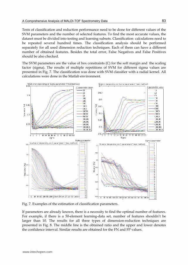
Tests of classification and reduction performance need to be done for different values of the

SVM parameters and the number of selected features. To find the most accurate values, the

dataset must be divided into testing and learning subsets. Classification calculations need to

be repeated several hundred times. The classification analysis should be performed

separately for all used dimension reduction techniques. Each of them can have a different

number of obtained features. Besides the total error, False Negatives and False Positives

should be also checked.

The SVM parameters are the value of box constraints (C) for the soft margin and the scaling factor (sigma). The results of multiple repetitions of SVM for different sigma values are presented in Fig. 7. The classification was done with SVM classifier with a radial kernel. All calculations were done in the Matlab environment.

Fig. 7. Examples of the estimation of classification parameters.

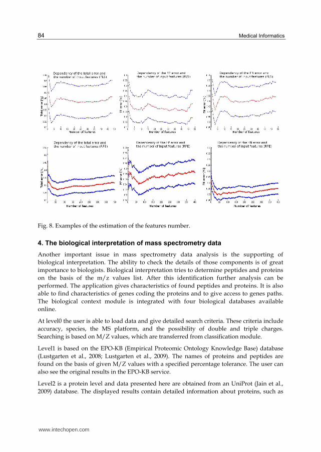
If parameters are already known, there is a necessity to find the optimal number of features.

For example, if there is a 50-element learning-data set, number of features shouldn’t be

larger than 10. The results for all three types of dimension-reduction techniques are

presented in Fig. 8. The middle line is the obtained ratio and the upper and lower denotes

the confidence interval. Similar results are obtained for the FN and FP values.

www.intechopen.com

Medical Informatics

84

Fig. 8. Examples of the estimation of the features number.

4. The biological interpretation of mass spectrometry data

Another important issue in mass spectrometry data analysis is the supporting of

biological interpretation. The ability to check the details of those components is of great

importance to biologists. Biological interpretation tries to determine peptides and proteins

on the basis of the m/z values list. After this identification further analysis can be

performed. The application gives characteristics of found peptides and proteins. It is also

able to find characteristics of genes coding the proteins and to give access to genes paths.

The biological context module is integrated with four biological databases available

online.

At level0 the user is able to load data and give detailed search criteria. These criteria include

accuracy, species, the MS platform, and the possibility of double and triple charges.

Searching is based on M/Z values, which are transferred from classification module.

Level1 is based on the EPO-KB (Empirical Proteomic Ontology Knowledge Base) database

(Lustgarten et al., 2008; Lustgarten et al., 2009). The names of proteins and peptides are

found on the basis of given M/Z values with a specified percentage tolerance. The user can

also see the original results in the EPO-KB service.

Level2 is a protein level and data presented here are obtained from an UniProt (Jain et al.,

2009) database. The displayed results contain detailed information about proteins, such as

www.intechopen.com

A Comprehensive Analysis of MALDI-TOF Spectrometry Data

85

entry name, status of reviewing process, organism, gene names and identifiers, features and

GO annotations. It is also possible to see the original results returned by the database.

Level3 is a genes level and it gives information about genes coding a particular protein

chosen at a previous level2. Presented data are based on NCBI service (Wheeler, 2009).

Searching is based on a gene identifier and it returns precise information about a particular

gene, its role, status, lineage and related data. Level4 is based on gene pathways data. It is

integrated with the KEGG database (Kyoto Encyclopedia of Genes and Genomes) (Kanehisa,

2008). Level 4 gives details about gene pathways, structures, sequences, and references to

other databases.

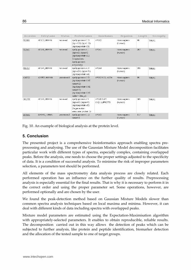
An example of biological results obtained at the level of proteins is presented in Fig. 10.

More results of the analysis performed on real data are presented in (Plechawska-Wojcik,

2011a).

Fig. 9. Schema of a biological-interpretation module.

www.intechopen.com

Medical Informatics

86

Fig. 10. An example of biological analysis at the protein level.

5. Conclusion

The presented project is a comprehensive bioinformatics approach enabling spectra pre-

processing and analysing. The use of the Gaussian Mixture Model decomposition facilitates

particular work with different types of spectra, especially complex, containing overlapped

peaks. Before the analysis, one needs to choose the proper settings adjusted to the specificity

of data. It is a condition of successful analysis. To minimise the risk of improper parameters

selection, a parameters test should be performed.

All elements of the mass spectrometry data analysis process are closely related. Each

performed operation has an influence on the further quality of results. Preprocessing

analysis is especially essential for the final results. That is why it is necessary to perform it in

the correct order and using the proper parameter set. Some operations, however, are

performed optionally and are chosen by the user.

We found the peak-detection method based on Gaussian Mixture Models slower than

common spectra analysis techniques based on local maxima and minima. However, it can

deal with different kinds of data including spectra with overlapped peaks.

Mixture model parameters are estimated using the Expectation-Maximisation algorithm

with appropriately-selected parameters. It enables to obtain reproducible, reliable results.

The decomposition carried out in this way allows the detection of peaks which can be

subjected to further analysis, like protein and peptide identification, biomarker detection

and the allocation of the tested sample to one of target groups.

www.intechopen.com

A Comprehensive Analysis of MALDI-TOF Spectrometry Data

87

Classification allows the initial indication of the power of the predictive model and the functional analysis of detected peaks. It is, however, a difficult task, due to the high dimensionality and feature correlation. Many thousands of features and tens of objects require two-step dimensionality reduction. The first one is based on the Gaussian mask, imposed on all spectra of the dataset. The second is the separation of the most informative features, conducted by the dimensionality-reduction techniques. Due to the high correlation degree, the classification should be based on features. Before the classification procedure the classifier parameters need to be specified.

The last step of the analysis is the biological interpretation. Biological databases integration facilitates the verification of the results. This test is important because of the possible False Discovery Rate obtained during the raw spectra analysis and classification. Such verification gives the possibility to verify the analysis from another angle. Biological analysis based on several external databases gives reliable functional analysis. Source databases are updated frequently. This ensures reliable, actual results.

6. Acknowledgment

The author is grateful to Prof. Joanna Polańska for inspiration, many invaluable suggestions and assistance in the preparation of this paper.

7. References

Akaike, H. (1974). A new look at the statistical model identification. IEEE Transactions on

Automatic Control, 9, pp. 716–723.

Banfield, J. & Raftery, A. (1993). Model-based gaussian and non-gaussian clustering.

Biometrics, 49, p.803–821.

Barnhill, S.; Vapnik, V.; Guyon, I. & Weston, J. (2002). Gene selection for cancer classification

using support vector machines. Machine Learning, 46, pp. 389–422.

Boulesteix, A. (2004). PLS dimension reduction for classification with high-dimensional

microarray data. StatAppl GenetMol Biol, 3, pp. 33.

Boulesteix, A. & Strimmer, K. (2006). Partial least squares: a versatile tool for the analysis of

high-dimensionalgenomic data. Briefings In Bioinformatics, 8(1), pp. 32-44.

Bozdogan, H. (1990). On the information-based measure of covariance complexity and its

application to the evaluation of multivariate linear models. Communications in

Statictics, Theory and Methods, 19, p. 221–278.

Bozdogan, H. (1993) Choosing the number of component clusters in the mixture-model

using a new informational complexity criterion of the inverse-fisher informational

matrix. Springer-Verlag,Heidelberg, 19, pp. 40–54.

Celeux G. & Soromenho G. (1996). An entropy criterion for assessing the number of clusters

in a mixture model. Classification Journal, 13, pp. 195–212.

Coombes, K.; Baggerly, K. & Morris, J. (2007). Pre-processing mass spectrometry data.

Fundamentals of Data Mining in Genomics and Proteomics, in : W. Dubitzky, M.

Granzow, and D. Berrar, (Eds.), pp. 79-99, Kluwer, Boston.

Cwik, J. & Koronacki, J. (2008). Statisitical learining systems. Akademicka Oficyna

Wydawnicza Exit Warszawa, pp. 239-245.

www.intechopen.com

Medical Informatics

88

Dempster, A.P.; Laird, N.M. & Rubin D.B. (1977). Maximum likelihood from incomplete

data via the em algorithm. J. R. Stat. Soc., 39,1:1—38.

Du, P.; Kibbe, W. & Lin S. (2006). Improved peak detection in mass spectrum by

incorporating continuous wavelet transform-based pattern matching.

Bioinformatics, Vol. 22 no. 17 2006, 2059-2065.

Eidhammer, I.; Flikka, K.; Martens L. & Mikalsen S. (2007). Computational methods for mass

spectrometry proteomics, John Wiley and sons.

Everitt B.S. & Hand D.J. (1981). Finite Mixture Distributions, Chapman and Hall, New York.

Fort, G. & Lambert-Lacroix, S. (2005). Classification using partial least squares with

penalized logistic regression. Bioinformatics, 21(7), pp. 1104–1111.

Fung, E.T. & Enderwick C. (2002) ProteinChip clinical proteomics: computational challenges

and solutions, Biotechniques, Suppl., 32, pp. 34-41.

Garthwaite, P.H. (1994). An interpretation of partial least squares. J. Amer. Statist. Assoc., 89,

pp. 122–127.

Guindani, M.; Do, K.; Mueller, P. & Morris, J. (2006). Bayesian Mixture Models for Gene

Expression and Protein Profiles. Bayesian Inference for Gene Expression and

Proteomics. KA Do, P Mueller, M Vannucci (Eds.) New York: Cambridge University

Press, pp. 238-253.

Huang, X.; Pan, W.; Grindle, S.; et al. (2005). A comparative study of discriminating human

heart failure etiology using gene expression profiles. BMC Bioinformatics, 6, pp. 205.

Jain, E.; Bairoch, A.; Duvaud, S.; Phan, I.; Redaschi, N.; Suzek, B.E.; Martin, M.J.; McGarvey,

P. & Gasteiger E. (2009). Infrastructure for the life sciences: design and

implementation of the UniProt website. BMC Bioinformatics 10, pp. 136.

Kanehisa, M.; Araki, M.; Goto, S.; Hattori, M.; Hirakawa, M.; Itoh, M.; Katayama, T.;

Kawashima, S.; Okuda, S.; Tokimatsu, T. & Yamanishi, Y. (2008). KEGG for linking

genomes to life and the environment. Nucleic Acids Res., 36, D480-D484.

Liu, Y. & Rayens, W. (2007). PLS and dimension reduction for classification. Computational

Statistics, 22, pp. 189–208.

Lustgarten, J.L.; et al. (2008). EPO-KB: a searchable knowledge base of biomarker to protein

links. Bioinformatics, 24(11), pp. 1418-1419.

Lustgarten, J.L.; et al. (2009). Knowledge-based variable selection for learning rules from

proteomic data. Bioinformatics, 10(Suppl 9), S16.

Man, M.Z.; Dyson G.; Johnson K., et al. (2004). Evaluating methods for classifying

expression data. J Biopharm Stat, 14, 1065–84.

Mantini, D.; Petrucci, F., Del Boccio, P.; Pieragostino, D.; Di Nicola, M.; Lugaresi, A.;

Federici, G.; Sacchetta, P.; Di Ilio, C. & URBANI A. (2008). Independent component

analysis for the extraction of reliable protein signal profiles from MALDI-TOF mass

spectra, Bioinformatics, 24, 63-70.

Mantini, D.; Petrucci, F.; Pieragostino, D.; Del Boccio, P.; Di Nicola, M.; Di Ilio, C.; Federici,

G.; Sacchetta, P.; Comani, S. & URBANI A. (2007) LIMPIC: a computational method

for the separation of protein signals from noise, BMC Bioinformatics, 8, 101.

Mao, J.; Jain, A.K. & Duin, R.P.W. (2000). Statistical pattern recognition: a review. IEEE

Trans. PAMI, 22(1): pp. 4–37.

www.intechopen.com

A Comprehensive Analysis of MALDI-TOF Spectrometry Data

89

Morris, J.; Coombes, K.; Kooman, J.; Baggerly, K. & Kobayashi, R. (2005) Feature extraction

and quantification for mass spectrometry data in biomedical applications using the

mean spectrum. Bioinformatics, 21(9), pp. 1764-1775.

Nguyen, D. & Rocke D. Tumor classification by partial least squares using microarray gene

expression data. Bioinformatics, 18, pp. 39–50.

Nguyen, D. & Rockeb, D. (2004). On partial least squares dimension reduction for

microarray-based classification: a simulation study. Computational Statistics & Data

Analysis, 46, pp. 407–425.

Plechawska, M. (2008a). Comparing and similarity determining of Gaussian distributions

mixtures. Polish Journal of Environmental Studies, Vol.17, No. 3B, Hard Olsztyn, pp.

341-346.

Plechawska, M. (2008b). Using mixtures of Gaussian distributions for proteomic spectra

analysis, International Doctoral Workshops, OWD 2008 Proceedings, pp. 531-536.

Polanska, J.; Plechawska, M.; Pietrowska, M. & Marczak, L. (2011). Gaussian Mixture

decomposition in the analysis of MALDI-ToF spectra. Expert Systems, doi:

10.1111/j.1468-0394. 2011. 00582.x, 2011.

Plechawska-Wójcik M. (2011a). Biological interpretation of the most informative peaks in the

task of mass spectrometry data classification. Studia Informatica. Zeszyty Naukowe

Politechniki Śląskiej, seria INFORMATYKA. Vol.32, 2A (96). Wydawnictwo

Politechniki Śląskiej, 2011, pp. 213-228.

Plechawska-Wójcik M. (2011b). Comprehensive analysis of mass spectrometry data – a case

study. Contemporary Economics. Univeristy of Finanse and Management in Warsaw.

Randolph, T.; Mithcell, B.; Mclerran, D.; Lampe, P. & Feng Z. (2005). Quantifying peptide

signal in MALDI-TOF mass spectrometry data. Molecular & cellular proteomics,

MCP, 4 (12), pp. 1990-9.

Schwarz, G. (1978). Estimating the dimension of a model. Annals of Statistics, 6, p. 461–464.

Stapor, K. (2005). Automatic objects classification. Akademicka Oficyna Wydawnicza Exit

Warszawa, pp. 35-52.

Tibshirani, R.; Hastiey, T.; Narasimhanz, B.; Soltys, S.; Shi, G.; Koong A. & Le, Q.T. (2004)

Sample classification from protein mass spectrometry, by 'peak probability

contrasts'. Bioinformatics, 20, pp. 3034 - 3044.

Vapnik, V.; Boster, B. & Guyon, I. (1992). A training algorithm for optimal margin classifiers.

Fifth Annual Workshop on Computational Learning Theory, pp. 114–152.

Vapnik, V. (1995). The Nature of Statistical Learning Theory. Springer.

Vapnik, V. (1998). Statistical Learning Theory. Wiley.

Wheeler DL et al. (2009). Database resources of the National Center for Biotechnology

Information. Nuc. Acids Res., 37, D5-D15.

Windham, M.P. & Cutler A. (1993). Information ratios for validating cluster analyses. Journal

of the American Statistical Association, 87:1188–1192.

Wold, H. (1996). Estimation of principal components and related models by iterative least

squares. Multivariate Analysis, Academic Press, New York, pp. 391-420.

Yasui, Y.; Pepe, M.; Thompson, M.L.; Adam, B.L.; Wright, Y. Qu.; Potter, J.D.; Winget, M.;

Thornquist M. & Feng Z. (2003). A data-analytic strategy for protein biomarker

discovery: profiling of highdimensional proteomic data for cancer detection.

Biostatistics, 4, pp. 449-463.

www.intechopen.com

Medical Informatics

90

Zhang, S.Q.; Zhou, X.; Wang, H.; Suffredini, A.; Gonzales, D.; Ching, W.K.; Ng, M. & Wong

S. (2007). Peak detection with chemical noise removal using Short-Time FFT for

a kind of MALDI Data, Proceedings of OSB 2007, Lecture Notes in Operations

Research, 7, pp. 222-231.

www.intechopen.com

Medical InformaticsEdited by Prof. Shaul Mordechai

ISBN 978-953-51-0259-5Hard cover, 156 pagesPublisher InTechPublished online 09, March, 2012Published in print edition March, 2012

InTech EuropeUniversity Campus STeP Ri Slavka Krautzeka 83/A 51000 Rijeka, Croatia Phone: +385 (51) 770 447 Fax: +385 (51) 686 166www.intechopen.com

InTech ChinaUnit 405, Office Block, Hotel Equatorial Shanghai No.65, Yan An Road (West), Shanghai, 200040, China

Phone: +86-21-62489820 Fax: +86-21-62489821

Information technology has been revolutionizing the everyday life of the common man, while medical sciencehas been making rapid strides in understanding disease mechanisms, developing diagnostic techniques andeffecting successful treatment regimen, even for those cases which would have been classified as a poorprognosis a decade earlier. The confluence of information technology and biomedicine has brought into itsambit additional dimensions of computerized databases for patient conditions, revolutionizing the way healthcare and patient information is recorded, processed, interpreted and utilized for improving the quality of life.This book consists of seven chapters dealing with the three primary issues of medical information acquisitionfrom a patient's and health care professional's perspective, translational approaches from a researcher's pointof view, and finally the application potential as required by the clinicians/physician. The book covers modernissues in Information Technology, Bioinformatics Methods and Clinical Applications. The chapters describe thebasic process of acquisition of information in a health system, recent technological developments inbiomedicine and the realistic evaluation of medical informatics.

How to referenceIn order to correctly reference this scholarly work, feel free to copy and paste the following:

Malgorzata Plechawska-Wojcik (2012). A Comprehensive Analysis of MALDI-TOF Spectrometry Data, MedicalInformatics, Prof. Shaul Mordechai (Ed.), ISBN: 978-953-51-0259-5, InTech, Available from:http://www.intechopen.com/books/medical-informatics/a-comprehensive-analysis-of-maldi-tof-spectrometry-data

© 2012 The Author(s). Licensee IntechOpen. This is an open access articledistributed under the terms of the Creative Commons Attribution 3.0License, which permits unrestricted use, distribution, and reproduction inany medium, provided the original work is properly cited.