Effectiveness of Smoke Barriers - Pressurised Stair Enclosur

A comparison of pressurised cylinders in
HIP systems using CFD and FEM
Lisa Lindqvist
Mechanical Engineering, master's level
2021
Luleå University of Technology
Department of Engineering Sciences and Mathematics

LULEÅ UNIVERSITY OF TECHNOLOGY
DEPARTMENT OF ENGINEERING SCIENCES AND MATHEMATICS
A comparison of pressurised cylinders in HIPsystems using CFD and FEM
AUTHOR
ACADEMIC SUPERVISOR
INDUSTRIAL SUPERVISOR
Lisa LindqvistProf. Hans-Åke HäggbladPhD. Per Burström & M.Sc. Anton Fritz
October 6, 2021

Luleå University of Technology Lisa Lindqvist
Abstract
A hot isostatic press (HIP) is a system which utilises high temperatures and pressure in order to densifyand enhance the material properties of components in the aerospace, automotive and additive manufacturingindustries, to mention a few. Quintus is a world leading manufacturer of HIP systems, and this master’s thesiswork has been written in collaboration with them.
A HIP consists of a cylinder which gets filled with an inert gas, a gas which is then pressurised using compressors.Inside of the cylinder are heaters which ensure that the gas and load reach the desired temperature. Quintus’HIP construction has a wire wound cylinder. This means that a pre-stressed wire is wound around the cylinderfor a number of laps, resulting in the cylinder always being in a compressive stress state, thus ensuring a safeconstruction if a crack were to propagate in the material. This construction also allows for a more slim design ofthe cylinder which is beneficial when the gas is to be cooled, as the heat gets transported through the cylinder.An alternative design to this wire wound cylinder is a so called monoblock cylinder. This is a solid, thicker,cylinder, not wound by any wire. Quintus does not manufacture the monoblock HIP system, but these HIPs areon the market and therefore Quintus is keen to learn more about them.
In this work, differences in the cooling capabilities with respect to the cylinders’ strength has been investigated,regarding the wire wound and monoblock cylinders. This has been done by the means of CFD and FEM(ANSYS CFX and ANSYS Mechanical), where a simplified 2D axisymmetric model of each HIP version wasused. In CFX, both a steady state and transient simulation was run for each model in order to capture the coolingof the gas. The resulting temperature load on the cylinder was then exported to the Mechanical setup to solvefor the arising stresses of the cylinders.
The results of the work showed that the wire wound HIP does indeed exceed the monoblock cylinder when itcomes to the cooling rate, especially after some time when the gas has cooled off. Neither one of the cylinderswere at risk of yielding, and the monoblock cylinder was calculated to withstand >20 000 cycles, which is alsothe fatigue life of the wire in Quintus’ HIPs. The models and boundary conditions used in this work weresubjected to approximations, but the results obtained have still brought a lot of new insights to the monoblockconstruction, and have provided a good foundation for further analyses.
i

Luleå University of Technology Lisa Lindqvist
Acknowledgements
I would like to give my gratitude to my industrial supervisors, Dr. Per Burström and Anton Fritz, for theircontinuous support and helpfulness from start to finish of this master’s thesis. They have provided inputs andknowledge which has been most useful throughout the project.
In addition, I would also like to thank the remaining employees at Quintus Technologies for making me feelwelcome, and for showing interest in my work. I am especially grateful for the support and knowledge providedby Roger Andersson and Linda Fridlund when I was constructing the FEM models of the HIPs.
Last but not least, I am thankful for my academic supervisor, Prof. Hans-Åke Häggblad, for giving inputs onmy progress and always being easy to reach. I am also deeply thankful for the support and joyfulness given bymy friends at Luleå University of Technology. Not only during the time of this thesis work, but throughout allfive years of my studies.
ii

Luleå University of Technology Lisa Lindqvist
TABLE OF CONTENTS
Abstract i
Acknowledgements ii
Nomenclature
1 Introduction 11.1 Hot isostatic pressing . . . . . . . . . . . . . . . . . . . . . . . . . . . . . . . . . . . . . . . . 1
1.1.1 Wire wound & monoblock HIPs . . . . . . . . . . . . . . . . . . . . . . . . . . . . . . 21.2 Problem description and objectives . . . . . . . . . . . . . . . . . . . . . . . . . . . . . . . . . 41.3 Previous work . . . . . . . . . . . . . . . . . . . . . . . . . . . . . . . . . . . . . . . . . . . . 51.4 Delimitations . . . . . . . . . . . . . . . . . . . . . . . . . . . . . . . . . . . . . . . . . . . . 6
2 Theory 72.1 Quintus’ HIP construction . . . . . . . . . . . . . . . . . . . . . . . . . . . . . . . . . . . . . 7
2.1.1 Gas flow . . . . . . . . . . . . . . . . . . . . . . . . . . . . . . . . . . . . . . . . . . 72.2 Computational fluid dynamics . . . . . . . . . . . . . . . . . . . . . . . . . . . . . . . . . . . 8
2.2.1 Governing equations . . . . . . . . . . . . . . . . . . . . . . . . . . . . . . . . . . . . 92.2.2 Navier Stokes approximations . . . . . . . . . . . . . . . . . . . . . . . . . . . . . . . 102.2.3 Turbulence models . . . . . . . . . . . . . . . . . . . . . . . . . . . . . . . . . . . . . 112.2.4 Boundary layer modelling . . . . . . . . . . . . . . . . . . . . . . . . . . . . . . . . . 112.2.5 Buoyancy . . . . . . . . . . . . . . . . . . . . . . . . . . . . . . . . . . . . . . . . . . 12
2.3 Finite element method . . . . . . . . . . . . . . . . . . . . . . . . . . . . . . . . . . . . . . . 122.4 Fluid-structure interaction . . . . . . . . . . . . . . . . . . . . . . . . . . . . . . . . . . . . . 12
3 Method 143.1 Validation study . . . . . . . . . . . . . . . . . . . . . . . . . . . . . . . . . . . . . . . . . . . 14
3.1.1 Geometry and experimental setup . . . . . . . . . . . . . . . . . . . . . . . . . . . . . 143.1.2 Numerical outputs . . . . . . . . . . . . . . . . . . . . . . . . . . . . . . . . . . . . . 163.1.3 Meshing . . . . . . . . . . . . . . . . . . . . . . . . . . . . . . . . . . . . . . . . . . 173.1.4 Boundary conditions and solver settings . . . . . . . . . . . . . . . . . . . . . . . . . . 17
3.2 CFD modelling of HIPs . . . . . . . . . . . . . . . . . . . . . . . . . . . . . . . . . . . . . . . 183.2.1 Simplifications and assumptions . . . . . . . . . . . . . . . . . . . . . . . . . . . . . . 183.2.2 Wire wound 2D . . . . . . . . . . . . . . . . . . . . . . . . . . . . . . . . . . . . . . . 193.2.3 Monoblock 2D . . . . . . . . . . . . . . . . . . . . . . . . . . . . . . . . . . . . . . . 213.2.4 Meshing . . . . . . . . . . . . . . . . . . . . . . . . . . . . . . . . . . . . . . . . . . 223.2.5 Boundary conditions and solver settings . . . . . . . . . . . . . . . . . . . . . . . . . . 25
3.3 FEM analyses of cylinders . . . . . . . . . . . . . . . . . . . . . . . . . . . . . . . . . . . . . 263.3.1 Verification . . . . . . . . . . . . . . . . . . . . . . . . . . . . . . . . . . . . . . . . . 283.3.2 Fatigue analyses . . . . . . . . . . . . . . . . . . . . . . . . . . . . . . . . . . . . . . 28
4 Results 294.1 Validation study . . . . . . . . . . . . . . . . . . . . . . . . . . . . . . . . . . . . . . . . . . . 294.2 Wire wound HIP . . . . . . . . . . . . . . . . . . . . . . . . . . . . . . . . . . . . . . . . . . 30
4.2.1 CFD . . . . . . . . . . . . . . . . . . . . . . . . . . . . . . . . . . . . . . . . . . . . . 304.2.2 FEM . . . . . . . . . . . . . . . . . . . . . . . . . . . . . . . . . . . . . . . . . . . . 37
4.3 Monoblock HIP . . . . . . . . . . . . . . . . . . . . . . . . . . . . . . . . . . . . . . . . . . . 42

Luleå University of Technology Lisa Lindqvist
4.3.1 CFD . . . . . . . . . . . . . . . . . . . . . . . . . . . . . . . . . . . . . . . . . . . . . 434.3.2 FEM . . . . . . . . . . . . . . . . . . . . . . . . . . . . . . . . . . . . . . . . . . . . 46
4.4 Results comparison . . . . . . . . . . . . . . . . . . . . . . . . . . . . . . . . . . . . . . . . . 484.4.1 CFD . . . . . . . . . . . . . . . . . . . . . . . . . . . . . . . . . . . . . . . . . . . . . 494.4.2 FEM . . . . . . . . . . . . . . . . . . . . . . . . . . . . . . . . . . . . . . . . . . . . 51
5 Discussion 535.1 Validation study . . . . . . . . . . . . . . . . . . . . . . . . . . . . . . . . . . . . . . . . . . . 535.2 CFD . . . . . . . . . . . . . . . . . . . . . . . . . . . . . . . . . . . . . . . . . . . . . . . . . 53
5.2.1 Methodology . . . . . . . . . . . . . . . . . . . . . . . . . . . . . . . . . . . . . . . . 545.2.2 Results . . . . . . . . . . . . . . . . . . . . . . . . . . . . . . . . . . . . . . . . . . . 55
5.3 FEM . . . . . . . . . . . . . . . . . . . . . . . . . . . . . . . . . . . . . . . . . . . . . . . . . 565.3.1 Methodology . . . . . . . . . . . . . . . . . . . . . . . . . . . . . . . . . . . . . . . . 565.3.2 Results . . . . . . . . . . . . . . . . . . . . . . . . . . . . . . . . . . . . . . . . . . . 57
5.4 General . . . . . . . . . . . . . . . . . . . . . . . . . . . . . . . . . . . . . . . . . . . . . . . 57
6 Conclusions 59
7 Future Work 60
8 References 61
Appendix A Water cooling channel models i
Appendix B Monoblock Case 2 results iii
Appendix C Larger HIP model results v

1 Introduction Luleå University of Technology
1 Introduction
This work has been performed at Quintus Technologies in Västerås, Sweden, and is a master’s thesis in themechanical engineering program at Luleå University of Technology.
Quintus is a world leading company in the field of high pressure technologies, and stems back to the 1950swhen they first applied their technology on manufacturing synthetic diamonds [1]. The high-pressure businesswas rapidly expanded as the application areas increased. Today, Quintus is an international company and isrepresented in 35 countries around the globe [2].
One of Quintus’ main business areas is the manufacturing of hot isostatic presses (HIPs for short). This is aproduct used in a variety of industries, where the aim is to improve the material properties of components byexposing them to high temperatures and pressure for a period of time. Although Quintus is world leading, thereare other companies who are involved in the HIP industry. The HIPs manufactured by Quintus are not consistentwith all other constructions on the market, and this is where this thesis work come into play. By utilizing thecomputational tools of CFD and FEM, this work will investigate how the Quintus’ HIP construction measureagainst an alternative design which is found on the market.
In the upcoming section is a more thorough description of what a HIP is and how it operates. Next followssome more background and objectives of this thesis, and lastly is a presentation of previous works that are ofrelevance to this work, together with what delimitations the project will face.
1.1 Hot isostatic pressing
A hot isostatic press is an equipment used to densify components of different sizes and materials, most commonlymetals and ceramics [3]. The densification of the components is done by exposing them to high pressureisostatically, meaning that the pressure is applied from all directions. To achieve this the components are placedinside of the HIP, which is constructed as a cylinder, and the cylinder is then pressurized.
There are multiple areas where the use of hot isostatic pressing is of interest. These areas include all manufacturerswho seek to obtain components with 100% of their theoretical density and thus achieve longer lifetime, enhancedmaterial properties and other beneficial results [4]. The aerospace and additive manufacturing industry are justtwo examples where HIP is widely used [5].
The HIP process works by simultaneously exposing the components to high temperature and pressure.Temperatures above 1000 ◦C and pressures above 1000 bar are usually needed in order to achieve satisfactoryresults [3]. The exact temperature and pressure applied, and the time at which these quantities are held, varydepending on the desired final material properties of the components.
The pressure that is being applied places high demands on the construction of the HIP. In Figure 1, an overviewof the internal structure can be seen. In the center there is a workpiece (the component(s) to be densified), alsoreferred to as the load. Next is the furnace that heats up the interior of the HIP, followed by an insulation mantlethat reduces power consumption by maintaining the heat in the desired area, and protects the high pressurecylinder from high temperatures [3].
1

1 Introduction Luleå University of Technology
Figure 1: A simplified overview of the structure of a hot isostatic press [3].
To pressurize the HIP an inert gas is used, the most common one being argon. When the cylinder has beendrained of air and filled with argon it is pressurized using a compressor. Next the furnace heats up the gas andload, and further increases the pressure due to the temperature rise [3].
In a HIP cycle there are three main phases in general. First is a heating phase where the temperature and pressureis being built up to the desired level. Next is the holding phase where the temperature and pressure is constantfor a certain amount of time. Lastly is the cooling phase which releases the pressure and lowers the temperaturebefore the components in the HIP can be retrieved. The heat from the gas is transported through the cylinderwall, which subjects the cylinder to thermal stresses. Because of this, the cylinder often has some additionalcooling configuration to not risk yielding the cylinder.
Once the components have been subjected to the heat and pressure for a certain amount of time, the resultingoutcome is components that are more ductile, have no porosity and that have better fatigue properties, etc [3].
1.1.1 Wire wound & monoblock HIPs
What separates the HIPs manufactured by Quintus from many other manufacturer’s is the construction of thepressurised cylinder. Quintus’ cylinders are wire wound which means that a metal wire of a certain dimensionhas been wrapped around the HIP in a number of laps in order to withstand the high pressure. The wire ispre-stressed when winding which results in the cylinder always being subjected to compressive stresses duringall stages of the HIP process [6].
The second kind of cylinder used in HIP constructions is referred to as monoblock. This consists of a solid thickwalled cylinder which, in contrast to the wire wound cylinder, will experience tensile stresses during the HIPprocess [6]. In Figure 2, the difference between the wire wound and monoblock cylinder can be seen, both with
2

1 Introduction Luleå University of Technology
and without pressure applied.
Figure 2: Top: Monoblock cylinder. Bottom: Wire wound cylinder. Left: No pressure applied. Right:Pressure applied. [6].
Regarding the safety aspect, the wire wound cylinder has an advantage since, if a failure occurs, it is a so called”leak before burst” situation. This means that the gas inside the HIP will dissipate through the wire, and notcause a sudden rupture. The monoblock cylinder on the other hand has a catastrophic failure mode which meansthat if a crack is initiated it will propagate, resulting in severe damages to the surroundings if not discovered intime [6].
Another factor, apart from the wire winding, that differentiates the HIPs manufactured by Quintus is thedevelopment and implementation of Uniform Rapid Cooling (URC) and Uniform Rapid Quenching (URQ).These technologies enable the total time of a HIP cycle to be considerably reduced, and for the user to performhigh pressure heat treatments of the components [6].
When implementing URC or URQ in the HIP process, the cooling phase is shortened. With URC, the gastemperature can be reduced by 100-300 ◦C/min, and with URQ up to 3000 ◦C/min. This allows more controlfor the user to achieve certain material properties and to get a higher work efficiency by having a shorter totalcycle time [6]. In Figure 3 is an illustration of how the cooling phase can be shortened when using URCcompared with conventional cooling.
3

1 Introduction Luleå University of Technology
Figure 3: An example of a HIP cycle which shows the difference of the cooling stage with and withoutuniform rapid cooling [6].
When the temperature inside of the HIP decreases rapidly, it subjects the cylinder to thermal loads as mentionedearlier. This is of great importance to regulate in order to not cause any damage to the cylinder. Quintus’ wirewound HIPs handle this by having water cooling channels in between the cylinder and the wire winding, whichhelps to cool down the cylinder. Monoblock cylinders can be cooled by, for example, having similar watercooling channels on the outside of the cylinder.
This summarizes the operation of a HIP in general terms. More detailed information about the process and thecooling stage, which is of relevance to the simulation models of this thesis work, is given in theory section 2.1.
1.2 Problem description and objectives
The objective of this master’s thesis is to investigate the difference between the two different types of cylindersthat were mentioned in the previous section; wire wound and monoblock. A comparison will be made betweena wire wound HIP produced by Quintus, and two different plausible constructions of HIPs with monoblockcylinders. The two cases of monoblock configurations that are of interest to investigate differs regarding theirmethods of cooling the cylinder. These methods are:
1. Cooling water channels with solid rods on the outside of the cylinder,
2. Cooling rods on the outside of the cylinder.
These wire wound versus monoblock comparisons will be made for two different standardised sizes of QuintusHIPs. In all upcoming methodology and results, the HIP referred to is the smaller version of the two. A shortsummary of the results for the larger version is given in appendix C.
The purpose is to find out how the heat is transported through the cylinder during the cooling phase using 2DCFD simulations. Considering that the rapid cooling will subject the cylinder to thermal stresses, there is anadditional interest in finding what maximum heat load is possible with regards to the strength of the cylinder bythe use of FEM.
To specify further, the main objectives of the thesis work will be to find:
4

1 Introduction Luleå University of Technology
• The temperature of the gas when exiting the cooling loop
• The heat distribution throughout the cylinder wall
• The transferred heat from the cylinder to the water
• The critical points with regards to the strength of the cylinder
• Modelling praxis and implications of using 2D models
The final aim is to be able to conclude what pros and cons exist for each cylinder type, and in what applicationareas either one can be beneficial to use.
1.3 Previous work
As a basis of this work lies mainly previous master’s theses conducted at Quintus Technologies. Since thereare few external studies done on the heat transfer in a HIP cylinder, these theses will be the main sources ofinformation for the numerical models that are to be constructed.
This thesis is in many ways a continuation of the work conducted by Jansson [7]. He investigated the heattransfer from the gas to the cylinder wall and cooling water in a HIP from Quintus, i.e. with a wire woundcylinder, by the use of CFD. He also coupled the CFD results with FEM to analyse the critical points in thecylinder with regards to the thermal stresses. His work thereby provides information about the CFD and FEMsimulation procedures applicable to this thesis work. Jansson performed 2D CFD simulations of the HIP withCFX as the solver. He implemented some simplifications to the model in order to reduce the computationalcost, but was still able to capture most of the gas flow path in the HIP. The model that is to be created in thiswork will be simplified even further than Jansson’s, but his work will still act as a valuable source.
The results obtained by Jansson from the CFD simulations were compared with measurements of the temperaturesinside of an operating HIP. From this he concluded that the simulation results were unable to fully resemblethe test data, but they were seen to follow the same pattern as the test data regarding the magnitude andtemperature distribution throughout the cylinder wall. The differences were believed to be caused by the modelsimplifications, and he thus suggests that a more detailed model of the inner region of the HIP and/or thewater cooling channels would be beneficial. His results of the FEM analyses were considered to provide someinformation about the cooling capabilities but needed more work to be fully credible.
Another work that provide experimental validation of the CFD simulations of a HIP is a master’s thesis conductedby Sjerling & Ramstedt [8]. They investigated the performance of the URQ process in a Quintus HIP bymeans of CFD. Though they performed experimental measurements of the temperature on the load inside ofthe furnace that were to be quenched, and therefore did not measure values that will be of relevance to thisthesis work. However they, as well as Jansson [7], created a 2D representation of the HIP, and managed to getsatisfactory results that were close to the experimental data for different materials and sizes of the load. Thustheir methodology of the 2D numerical HIP model shows to be a credible approach for simulating the heattransfer inside of a HIP. The deviations from the experimental results that could be found increased with thesize of the load, which was said to imply the importance of accurate thermal properties of the materials.
An external source that will be used is a study conducted by J.I. Córcoles et al. [9]. This work presentsexperimental results of the heat transfer in a double pipe heat exchanger and will be used to validate thenumerical methods that are to be used in the HIP simulations. The reason being that this work will not have the
5

1 Introduction Luleå University of Technology
possibility to conduct experiments to directly verify the results of the HIP simulations. A further description ofthe study and the validation procedure is given in section 3.1.
1.4 Delimitations
The most obvious limitation this project will face is the time constraint. In order to consider this the project willbe adjusted to limit computational requirements. This will make the simulation models less time consumingboth to set up and to solve. It also serves the purpose of simplifying the results analyses. Some simplificationswill also be implemented in order to protect confidential information provided by Quintus Technologies.
The main delimitations that will be applied to this project are thus:
• The computational power available is four CPU cores with 64 GB of RAM.
• The software that will be used is ANSYS CFX 2020 R2.
• The HIP’s complex geometry will be simplified and narrowed down, both to reduce the computationalcost and to make the results more easily interpreted.
• The simulations will be of a 2D slice since geometry and flow in the HIP is mainly axisymmetric.
• The wire winding, cooling closures and center of the HIP will not be included in detail in the model. Bothdue to computational cost and confidentiality.
6

2 Theory Luleå University of Technology
2 Theory
In this theory chapter, information is provided regarding the Quintus HIP construction, followed by details onthe computational resources upon which a large part of this master’s thesis is based.
2.1 Quintus’ HIP construction
Given in the introducing section 1.1 is some information about HIPs as well as general information on howthe wire wound HIP differs from a monoblock HIP. In this part follows some more facts about Quintus’ HIPs,applicable to the upcoming CFD and FEM model descriptions.
In order to be able to meet all customer demands who wish to HIP different components of different sizes, theHIPs are also produced in a variety of sizes. These can vary in a wide range, with many cylinders reaching afew meters in height. In this work two different sizes of HIPs will be analysed, where the larger one is around2 times larger than the smaller one. The main focus in the upcoming report lies with the smaller version of thetwo.
The wire wound HIPs by Quintus consist (in general) of the parts seen in Figure 4. The wire is pretensionedto keep the cylinder in a compressive stress state during all times of the HIP process. This allows for a moreslim design of the cylinder as it does not need to be dimensioned for withstanding tensile stresses. For the HIPsanalysed in this work, the fatigue life of the wire has been calculated to be above 20 000 cycles. In betweenthe wire and cylinder is the water cooling. This consists of vertical solid rods, with water flowing in betweenthem. With the help of the water the cylinder is kept at an acceptable temperature by both conducting away heatthrough the rods, and by convection through the water. Because of the cylinder’s relatively thin design, a highheat transfer rate is possible to achieve.
On the inside of the cylinders are two mantles, one inner and one outer. The inner mantle has the purpose ofinsulating the inner part of the HIP, thus keeping the heat concentrated in the hot zone where the load is placed,and protecting the cylinder from the high temperatures of the gas. With the gap between the inner and outermantle, a passage is created where the gas can pass.
2.1.1 Gas flow
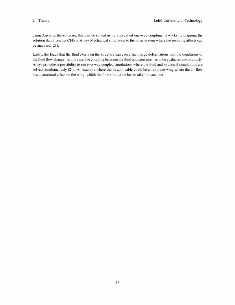
The gas can circulate inside of the HIP by flowing down in between the insulation mantle and bottom insulation,up along the gap in between the inner and outer mantle (inner cooling channel), and then down along the cylinderwall (outer cooling channel), where the gas is cooled off as the heat is transferred through the cylinder and awaywith the cooling water (see Figure 4). What drives the flow is depending on which stage the HIP process is in.During the holding stage, the flow is driven by natural convection as the temperature of the gas varies inside ofthe HIP. The heat is mainly contained in the inner part of the HIP during holding, as mentioned earlier. However,some of the heat can still leak through the insulation mantle as the material of the mantle is somewhat porous.In the cooling stage, the pumps are activated which increases the gas flow rate in the HIP and allows for cool airin the bottom of the HIP to circulate. This creates forced convection flow and thus a higher cooling rate of thegas. As the gas has passed the cylinder, some of it gets recirculated into the load area as it reaches the pumps.
When the gas has reached the upper closure area and makes its way out towards the cylinder, the majority of thegas will hit the cylinder wall around one area, giving rise to a local temperature hot spot in the cylinder. Thishot spot, together with other places in the HIP, are monitored using thermocouples (TCs). The TCs measuringthe cylinder hot spot is of additional importance since this temperature is not allowed to exceed a certain value.The limit exists to not risk the cylinder yielding due to the thermal load, but is set with a safety margin which
7

2 Theory Luleå University of Technology
means that the cylinder should in reality be able to withstand higher thermal loads.
Figure 4: An illustration of a cross section of a wire wound HIP. When the cooling stage is initialised, thepumps are activated and the gas flows along the mantles and down along the cylinder wall which aids intransferring away heat.
2.2 Computational fluid dynamics
In the field of fluid dynamics, one investigates the motion and interaction of fluids. With the help of computersand numerical simulations it is today possible to solve fluid flow problems of high complexity with a goodaccuracy [10], this is what is referred to as Computational Fluid Dynamics (CFD).
There are a variety of industries where CFD is an essential computational asset. Some examples are theaerospace, automotive and biomedical industries [10]. With the help of CFD, engineers can calculate the liftforce on airplanes, improve fuel efficiency on cars and predict how the blood flows in the human body, to justmention a few application areas.
Constructing a CFD setup requires a good understanding from the user of the problem at hand, and what physicsare involved. First, a geometric model is constructed representing the actual object/system. Next follows todivide the whole geometry into several subdomains (more commonly named elements/cells), and thus creatinga mesh. The cells in the mesh serve the purpose of acting as smaller computational domains on which thefluid flow properties are calculated numerically. The overall results are then presented as a combination of theindividual cell solutions.
The accuracy of the results are highly dependent on the resolution of the mesh. With more cells follows a moredense computation of the flow properties, and thus a more accurate result. Although the denser a mesh becomes,the longer computational times are required to produce a result.
8

2 Theory Luleå University of Technology
However, it is important that one does not trust the results blindly as soon as the results have become meshindependent (when they do not change with a refinement of the mesh), since another important part of the setupis the implementation of boundary conditions. The boundary conditions and solver settings control the physicsand other properties of the model, and are a crucial aspect to enter correctly as this will have an extensive impacton the end results.
The equations upon which CFD is built are presented in the upcoming subsection, followed by some details onmore specific areas of CFD.
2.2.1 Governing equations
As a foundation for the field of fluid dynamics lies the governing equations, most widely known as the NavierStokes equations [11]. The equations are all derived from three fundamental principles of physics: conservationof mass, conservation of momentum (Newton’s second law) and conservation of energy.
The first equation, the continuity equation, stems from the principle of conservation of mass. Considering asmall control volume which is fixed in space, and through which a fluid passes, the rate of change of fluid massinside the control volume has to equal the difference between the rate of mass entering and exiting the controlvolume [10]. The equation is expressed as (1).
∂ρ
∂t+
∂(ρu)∂x
+∂(ρv)
∂y+
∂(ρw)∂z
= 0, (1)
where ρ is the fluid’s density inside the control volume, and u,v,w are the velocities of the fluid in x,y,z Cartesiancoordinates respectively. Note that for incompressible flows, the density of the fluid remains constant inside thecontrol volume and thus the first term containing the density derivative with respect to time becomes 0.
The second part of the Navier Stokes equations (the momentum equation) once again consider the small controlvolume through which a fluid passes. Deriving from Newton’s second law, it follows that the sum of all forcesacting on the fluid in the volume has to equal the product of the volume’s mass and its acceleration.
ρDuDt
=∂σxx
∂x+
∂τyx
∂y+
∂τzx
∂z+∑Fx, (2)
ρDvDt
=∂τxy
∂x+
∂σyy
∂y+
∂τzy
∂z+∑Fy, (3)
ρDwDt
=∂τxz
∂x+
∂τyz
∂y+
∂σzz
∂z+∑Fz, (4)
with the left hand side being the product of the control volume’s mass (simplified to its density) and acceleration,and the right hand side being a summation of the internal forces and the external forces (Fi).
Lastly, the governing equations of fluid dynamics consider the conservation of energy for situations where heattransfer is present. The equation stems from the first law of thermodynamics, which states that the rate ofchange of energy in a system is equal to the sum of the net rate of heat added and the net rate of work done. Theresulting equation, after some derivation, is seen in (5).
ρDEDt
=∂
∂x
[λ
∂T∂x
]+
∂
∂y
[λ
∂T∂y
]+
∂
∂z
[λ
∂T∂z
]− ∂(up)
∂x− ∂(vp)
∂y− ∂(wp)
∂z+Φ, (5)
where E is the energy in the control volume, λ is the thermal conductivity, and Φ is a dissipation function whichdescribes the effects which the viscous stresses have on the energy equation.
9

2 Theory Luleå University of Technology
Equations (1) to (5) are hence the foundation upon which the field of fluid dynamics is based. The equationscan be derived further and/or simplified, depending on the characteristics of the flow. They also differ slightlydepending on if the infinitesimal control volume is fixed in space, which is the case in (1) to (5), or if the volumemoves together with the fluid [11].
In the upcoming subsections some central areas within fluid dynamics are presented and explained.
2.2.2 Navier Stokes approximations
One vital part of fluid dynamics is turbulence. Most flows studied are of turbulent nature, with the fluid movingin irregular patterns. This is in contrast to the fluid being laminar, where the particles of the fluid move indefined streamlines without interfering with other streamlines [12]. One factor which can provide an indicationif a flow is laminar or turbulent is the dimensionless Reynolds number. The number is calculated by
Re =ρLV
µ, (6)
with ρ being the density of the fluid, L is a so called characteristic length (this usually equals the length of thebody in which the fluid flows), V is the velocity of the flow and µ is the fluid’s dynamic viscosity [11]. Forflows with a Reynolds number lower than 2000, the flow is generally laminar. For Reynolds numbers between2000 and 3500 the flow is in a transitional state and above 3500 the flow is generally turbulent [12]. Notethat these numbers vary depending on the flow case, and should more be seen as an indication on the expectedcharacteristics of the flow.
The Navier Stokes equations ((1) to (5)) are possible to solve analytically when dealing with simple casesof laminar flow. If the flow is turbulent however, the equations become impossible to solve analytically, andquickly become very computationally demanding to solve numerically. For flows with low Reynolds numbersand with simple characteristics, it is possible to obtain an exact solution of the Navier Stokes equations, thismethod is called the Direct Numerical Simulation (DNS) [13]. However, most flow cases do not fulfill theserequirements and thus some approximations of the turbulence is necessary.
Following the DNS method is the LES (Large-Eddy Simulation) approach. This is a method founded on theprinciple that the turbulence on the small scale is of a more global character than the large scale turbulence,which is what transports the turbulent energy and is thus of greater interest to resolve [13]. By approximatingthe small scaled turbulence and resolving the large scale the LES-method obtains a solution less computationallydemanding than the DNS-method, but of lower accuracy.
The last approach, which is also the least computationally demanding one, is called Reynolds Averaged NavierStokes equations (RANS) [13]. This approach is the one most used in engineering, and is the one that will beused and focused on in this project. Thus the upcoming information and model descriptions are all based on theRANS turbulence approach.
The RANS method approximates all turbulence, both of small and large scale. The approximation is doneby time-averaging the Navier Stokes equations ((1) to (5)). By decomposing the velocities, pressure andtemperature into their mean and fluctuating components, a new unknown variable arises [10]. This variableis called the Reynolds stress, which in turn can be resolved in different ways depending on which so calledturbulence model is implemented. The different turbulence models are briefly described in the followingsubsection.
10

2 Theory Luleå University of Technology
2.2.3 Turbulence models
For resolving the Reynolds stress in a flow computed using the RANS equations, and thus approximatingthe turbulence of the flow, there are a numerous turbulence models which can be evaluated. Which one isthe most appropriate to use depends on how well, and where, the turbulence is wished to be captured. Withhigher accuracy follows higher computational requirements, as would be expected. Listed below are the mostcommonly used turbulence models, together with a brief explanation of each.
There are two main categories of turbulence models for the RANS equations, these are the Eddy-viscositymodels and the Reynolds stress models. For this thesis work, only the Eddy-viscosity models have beenconsidered and are therefore the ones which will be mentioned.
The two-equation k-ε model was the previous industrial standard [14] and is a simple and robust method. k isthe kinetic energy of the turbulence, and ε is the dissipation rate of the turbulence energy. The drawback of themethod is that it was developed for high Reynolds number flows and is thus not ideal for capturing low Reynoldsnumber- and near wall-flows. To resolve the near wall flow, so called wall functions can be implemented whichapproximates the near wall characteristics [15].
Next is the k-ω turbulence model, which in contrast to the k-ε model is able to resolve wall bounded flows [14],but is less robust when computing the free stream flow.
A model, which has come to be the industrial standard of today [14], is called SST k-ω. This model combinesthe perks of both the k-ε and k-ω model by switching between the two formulations depending on location inthe domain.
2.2.4 Boundary layer modelling
In computational fluid dynamics, the fluid layer closest to the adjacent solid wall is of great importance toresolve accurately. This is to ensure that the wall shear stress, surface pressure and forces are captured, whichin turn have an effect on flow separation, lift, etc [16].
The boundary layer consists of three main regions, namely the viscous sublayer, the log layer and the outer layer[16]. In the viscous sublayer, the flow is laminar and the velocity of the flow closest to the wall is zero. Movingon to the log layer, the flow transitions to being turbulent and the velocity increases, while it in the outer layeris fully turbulent.
To capture the velocity profile in the boundary layer, it requires a well structured density of the mesh nodesclosest to the surface. A value which is used to estimate the placement of the first node is called y+, which is adimensionless number and is calculated by
y+ =u∗yν
, (7)
with u∗ being the fluid’s friction velocity closest to the wall, y is the distance from the wall to the nearest nodeand ν is the kinematic viscosity of the fluid [17].
When constructing a mesh, one can either make it fine enough that the first node is located inside of the viscoussublayer, or place the first node in the log layer. Which alternative to choose is depending on the turbulencemodel and the available computational resources. The SST k-ω model for example is robust enough to resolvethe viscous sublayer and compute the velocities directly at the nodes, while the second alternative is favorablefor the k-ε method. Instead of resolving the viscous sublayer, the k-ε model uses a so called wall function toapproximate the velocity profile near the wall. This is a less computationally demanding approach, but can
11

2 Theory Luleå University of Technology
result in modelling errors depending on the flow conditions [16].
To resolve the viscous sublayer, a y+ ∼ 1 is recommended, and to enable the use of wall functions by placingthe first node in the log layer, a y+ > 30 is to aim for. Note that these values are a recommendation, and thatwith the development of the different CFD softwares it follows that a larger spectra of y+ is tolerable.
2.2.5 Buoyancy
Buoyant flow refers to when the flow is driven by natural convection, i.e. local density variations in the fluid.These variations can be caused by a number of factors such as local temperature variations, which in turn canarise from a heat source acting on the fluid.
The fluid can also be driven by mixed convection. In this case the flow is subjected both to a pressure gradient(forced convection), and buoyancy forces. To estimate the relevance of including buoyancy in ones model, theratio between Grashof and Reynolds number can be computed according to [18]
GrRe2 =
gβL∆TV 2 . (8)
In (8), g is the gravitational acceleration, β the thermal expansion coefficient, L the characteristic length, ∆T isthe temperature difference between the surface and bulk, and V is the fluid velocity. If the ratio approaches oris larger than 1, then this indicates that buoyancy is to be considered in the flow.
2.3 Finite element method
The finite element method (FEM) is a numerical method which has its origin in applied mathematics in the mid20th century [19]. Although, the most strongly associated application area of the finite element method is incomputational mechanics, which is the area of focus in this section.
The fundamental principle of FEM is to divide the geometry of interest into a finite amount of elements. Theelements are connected in points called nodes, and together the elements form a mesh. For each element, a setof integral formulations are evaluated, which stems from the governing differential equations of mass, force andenergy balance [19].
By defining materials, load conditions and boundary conditions for the geometry, the method delivers anapproximate numerical solutions to a numerous structural properties in the geometry. The properties can bedisplacement, velocity, stresses, strains, and many more. The use of FEM in structural mechanics requiresa good understanding of the underlying physics and strong computational resources, but can be applied in avariety of structural analyses, such as modal, buckling and fatigue analyses to mention a few [19].
2.4 Fluid-structure interaction
When dealing with problems that involve a coupling between fluid dynamics and structural mechanics one isstudying so called fluid-structure interactions (FSI). The fluid-structure interactions can be of differentcharacteristics depending on how the domains affect one another. It could be that the fluid only exerts minorforces on the structure, and the structure can thus be considered as rigid. An example of this is the blades inindustrial mixers being treated as rigid with respect to the fluid [20].
Another possibility is that the fluid has an affect on the structure in terms of pressure and/or thermal loads,but that the deformations of the structure are kept small enough that the fluid flow remains unaffected. When
12
2 Theory Luleå University of Technology
using Ansys as the software, this can be solved using a so called one-way coupling. It works by mapping thesolution data from the CFD or Ansys Mechanical simulation to the other system where the resulting affects canbe analysed [21].
Lastly, the loads that the fluid exerts on the structure can cause such large deformations that the conditions ofthe fluid flow change. In this case, the coupling between the fluid and structure has to be evaluated continuously.Ansys provides a possibility to run two-way coupled simulations where the fluid and structural simulations aresolved simultaneously [21]. An example where this is applicable could be an airplane wing where the air flowhas a structural effect on the wing, which the flow simulation has to take into account.
13

3 Method Luleå University of Technology
3 Method
In this chapter, the methodology of how the thesis work has been carried out is presented. First is the method ofthe validation study, conducted to establish credibility of the final results. In section 3.2 begins the presentationof the HIP modelling methods. First is the CFD method, and following this in section 3.3 is the method of theFEM analyses. Two sizes of HIPs were analysed in this thesis work. In this chapter though, the methodologyand figures presented are with regards to the smaller version. The same method was applied for the largerversion as well, with the only difference being the bulk element size of the mesh, and inlet flow conditions ofthe transient CFD analysis. The results of the wire wound/monoblock comparison for the larger version can befound in appendix C.
3.1 Validation study
The intention to use RANS-based turbulence models in the HIP simulations entails uncertainties regarding theirability to model the physics of the flow in an accurate way. In order to conclude that these turbulence modelsare indeed an appropriate approach, a validation study was performed.
Since the project aims to compute the heat transfer in a monoblock HIP, which Quintus do not manufacture,there is no possibility to validate the results against experimental data. There is also a lack of similar studiesthat could provide some insight to the expected results. The HIP models with wire wound cylinders, whichQuintus do indeed manufacture, are not possible to access fresh measurements from at the time this thesis waswritten. Thus the validation was conducted by studying and recreating a previous work done on a double pipeheat exchanger (DPHx). The report can be found in [9].
The DPHx studied in [9] provides similar conditions regardning the flow rate, Reynold’s number, density etc.as will be found in the HIP model with the pressurised argon. Therefore, if assuring that the turbulence modelscan accurately capture the physics of the DPHx, the reliability of the upcoming HIP simulations will increase.
In [9], 9 different cases of double pipe heat exchangers with slightly different geometries were simulatedusing Ansys Fluent, with the aim to obtain the heat transfer rate, friction factor, and other values that arepresented further ahead. Only the first case had a smooth inner tube, whereas the following cases had a spirallycorrugated inner tube. In this validation work, only the first case with a smooth inner tube will be numericallyrecreated. This is because it is the case with the highest similarity with the HIP, and [9] provides experimentalmeasurements of the temperature and pressure in the DPHx, which can be used for validation purposes.
The validation work was performed by creating a CFD model that resembled the experimental setup, usingthe same software that were to be used throughout the rest of the project (Ansys CFX). Since the simulationsdescribed in [9] were solved using Fluent as mentioned, and a few details were lacking in description, the setupof the simulations in CFX could not fully be resembled and some minor presumptions were thus made.
3.1.1 Geometry and experimental setup
The basic geometry and measurements of the DPHx can be seen in Figure 5, where the parts in blue representthe fluid (water) and the parts in grey are the pipes. Both the outer and inner pipe were made of stainless steel,and both had a thickness of 1.5 mm. The inner tube had a flow diameter of 22 mm, excluding the pipe thickness,and the corresponding diameter of the annular pipe was 35 mm.
14

3 Method Luleå University of Technology
Figure 5: The full geometry and basic measurements of the DPHx, with both the annular and inner pipeincluded as seen in grey. In blue are the fluid domains (water).
Since the DPHx model were to be solved using CFX, the interface between the hot and cold water could bemodelled using a ”thin material” instead of including the solid inner pipe in the model. Neither the annularpipe needed to be included since the outer walls were to be defined as adiabatic. Thus the final computationalgeometry that was used is the one found in Figure 6, where only the fluid domains are present. Note that theinner face of the annular flow was extruded inwards and filled the gap of the pipe. The outer diameters of thecold and hot water flow were thereby still 22 mm and 35 mm respectively.
Figure 6: The geometry of the hot and cold fluid domains that were used in computational purposes, wherethe solid pipes are not included.
The configuration of the heat exchanger was counter flow. Cold water flowed in the inner tube and hot water inthe opposite direction in the annulus [9].
The experiments, according to [9], were conducted by utilizing two 600 litre storage tanks with two variable-speedpumps, which allowed for the water to flow through the heat exchanger with different flow rates. The setup
15

3 Method Luleå University of Technology
included heating and cooling loops with capacities of 72 kW and 48 kW respectively, in order to maintain thedesired temperatures of the water that flowed through the heat exchanger. The inlet temperatures of both thecold and hot circuit were held constant at 22.1 ◦C and 60 ◦C. The experiment ended when it had reached steadystate, which was defined as when the temperatures at the outlets of both circuits did not fluctuate more than 0.06◦C for case 1, and 0.05 ◦C for case 2.
In order to obtain results from the experiments that could be comparable with the numerical ones, there werefour pressure sensors and four temperature sensors installed in the heat exchanger. These were mounted in theinlets and outlets of both the cold and hot water circuit, at a distance of 10D from the openings, with D beingthe flow diameter of the inner pipe (0.022 m).
A total of 8 experimental tests were carried out, 4 for case 1 and 4 for case 2 respectively. What separated these4 tests was the flow rate of the cold water, and thus also the Reynolds number of the cold circuit. Meanwhile,the flow rate of the hot water was held constant at 50 l/min through all tests. In Table 1 the conditions used foreach test can be seen. The same conditions were used in this validation work when setting up the simulations.
Table 1: The conditions used for the different tests that were carried out [9].
Test 1 Test 2 Test 3 Test 4Flow rate hot water [L min−1] 50 50 50 50Temperature hot water [◦C] 60 60 60 60Reynolds hot water 45000 45000 45000 45000Flow rate cold water [L min−1] 25 30 40 50Temperature cold water [◦C] 22.1 22.1 22.1 22.1Reynolds cold water 25000 30000 40000 50000
3.1.2 Numerical outputs
The pressure and temperature sensors that were mounted in the experimental heat exchanger providedmeasurements of pressure drop and temperatures that were then used to calculate the average heat transfer rate(Q), overall heat transfer coefficient (U) and Fanning friction factor (C f ) [9]. In order to obtain correspondingmeasurement data from the simulations, the area averaged pressure and temperature was extruded from thesame locations as the sensors, i.e. at 10D from the inlets and outlets.
The heat transfer rate Q was calculated by averaging Qh; the heat lost from the hot water domain, and Qc; theheat gained in the cold water domain. This was done since Qh and Qc could differ slightly due to minor lossesto the surroundings in the experiments, and numerical inconsistencies. The equations for calculating the heatloss and gain are given in (9) [9].
Qc = [mcp(Tout −Tin)]c , Qh = [mcp(Tin−Tout)]h , (9)
with m being the mass flow rate, cp the specific heat, Tin the temperature at the inlet and Tout at the outlet. Theindex c is the cold water domain and h the hot. Averaging (9) results in the heat transfer rate according to (10).
Q =Qh +Qc
2. (10)
The overall heat transfer coefficient U was calculated by
U =Q
As∆Tlm, (11)
16

3 Method Luleå University of Technology
where As is the surface area of the inner tube subjected to heat transfer, and ∆Tlm is the log mean temperaturedifference, given as
∆Tlm =∆T1−∆T2
ln(
∆T1∆T2
) , (12)
with ∆T1 and ∆T2 as∆T1 = Th,in−Tc,out ∆T2 = Th,out −Tc,in. (13)
Lastly the Fanning friction factor was calculated for the inner tube according to
C f =∆pD
2ρLpu2 , (14)
where ∆p is the pressure difference between the inlet and outlet of the cold water domain, D is the innerdiameter of the cold tube, ρ is the density of water, Lp is the length of the pressure section and u the averagewater velocity.
The above mentioned equations (10), (11) and (14) were calculated for the simulation results of each test foundin Table 1, and then compared with the given experimental results [9].
3.1.3 Meshing
In [9], a mesh independence study was performed for Case 1 and 2 in order to verify the accuracy of thenumerical results. Two different mesh resolutions were tested for each case, where the first mesh had 8 · 106
elements and the second one 20 ·106 elements. The study concluded that the simulations using the first, coarser,mesh delivered similar results as when using the second, finer, mesh. Thus the first mesh was used in all furthercase simulations.
In this validation work, a mesh consisting of 8·106 elements was constructed, motivated by the mesh independencestudy in [9]. The same mesh settings were used, which was a 3D tetrahedral unstructured mesh scheme with anelement size of 5 mm, and 18 inflation layers with a first layer thickness of 0.04 mm. Capture proximity wasalso switched on with 3 cells across gaps. The final mesh can be seen in Figure 7.
Figure 7: Mesh of the DPHx used in the validation study, consisting of 8 ·106 elements.
3.1.4 Boundary conditions and solver settings
The boundary conditions and setup described in [9] were used when setting up the DPHx model in CFX. Forthe inlets the flow rate and temperature according to Table 1 were assigned uniformly to the cold and hot siderespectively, with the flow rate recalculated to [kg/s]. Turbulence conditions were defined with an intensity of0.5% and an Eddy viscosity ratio of 1.
17

3 Method Luleå University of Technology
The outlets were defined as openings to allow for backflow, with a backflow turbulence intensity of 0.5% andEddy viscosity ratio of 1.
All walls were defined with a no-slip condition. The outer wall of the annulus pipe, as well as the outer wall atthe ends of the inner pipe not subjected to the annulus, were defined as adiabatic walls.
At the interface between the hot and cold water, a coupling heat transfer condition was set with the interfacebeing a thin material made of stainless steel with a thickness of 1.5 mm. The physical properties of stainlesssteel were collected as an average of the most common stainless steel types from [22].
For the working fluid water, its density ρ, viscosity µ, specific heat cp and thermal conductivity λ were given asfunctions of the temperature T as follows:
ρ(T ) = 386.0722+5.4014T −0.0147T 2 +1.1722 ·10−5T 3, (15)
µ(T ) = 0.0695−5.7412 ·10−4T +1.6025 ·10−6T 2−1.5028 ·10−9T 3, (16)
cp(T ) = 6889.4−22.4418T +0.0602T 2−5.1784 ·10−5T 3, (17)
λ(T ) =−1.5298+0.015T −3.3883 ·10−5T 2 +2.5651 ·10−8T 3. (18)
The simulations were solved for steady state. Both the advection scheme and turbulence numerics were solvedwith high resolution. The convergence criteria was set to an RMS target of 1e-5 and a conservation target of0.01.
In the post processing stage, the temperatures and pressures were measured at planes located 0.22 m from theinlets and outlets of the DPHx, to resemble the measurements obtained from the sensors in the experimentalsetup.
A total of four simulations were analysed, corresponding to each setup found in Table 1. The results andconclusions of the validation study can be found in section 4.1.
3.2 CFD modelling of HIPs
The analyses of the HIP cooling process were each divided into two simulations; one steady state-simulationand one transient. By running a steady state simulation the objective was to resemble the conditions in the outerchannel during the holding phase, when all conditions had stabilised. The results of the steady state simulationwere then used as initial conditions for the transient simulation, which in turn simulated the cooling phase andprovided the end results. This work process was repeated for each HIP model and geometry variation.
In the following sections, the general simplifications applicable to all HIP models are first mentioned. Next,the geometry and other descriptions of the wire wound and monoblock models respectively are described.Following this are some sections that are case independent; this being the meshing, boundary conditions andsolver settings. These sections are thus to be read with both the wire wound and monoblock models in mind,since the methodology did not differ significantly between them.
3.2.1 Simplifications and assumptions
Considering the aim of the project being to compare the heat transfer in two different kinds of cylinders, withdifferent cooling configurations, it follows that simplifications of the models is a necessity. This is for tworeasons; both in order to reduce the computational requirements and thus decrease the total simulation time,
18

3 Method Luleå University of Technology
and also to simplify the comparisons of the different models. Since all results will be analysed with respect tothe results of the corresponding cylinder, it is not the absolute values that are of interest. Thus it is justified toimplement simplifications and not include a high amount of details regarding the geometry and flow description,etc.
The main simplifications that are applicable to all models in this project are listed below:
• The top and bottom closures are excluded, and only the outer cooling channel is modelled. This is becausethe inner channel and closures are considered to be superfluous as the main focus lies on analysing theheat transfer between the gas and cylinder.
• The argon gas is assumed to have a constant pressure during the entire cooling phase, and for the gas inleta constant mass flow rate and temperature is assumed. In reality these variables vary during the coolingphase, but for comparison purposes it is considered to be adequate to use constant mean values whichyield the highest allowed thermal load on the cylinder.
• The geometry is a 2◦ slice of the full HIP. Since the HIP to a large extent is axisymmetric, it is sufficientto run a 2D axisymmetric simulation. In CFX this is handled by creating a slice of the geometry andapplying a mesh that is one element thick in the tangential direction.
• The argon gas inlet is extended a distance of 10D, with D being the diameter of the inlet. This is to aimfor a fully developed flow before the 90◦ bend, see Figure 9.
Other simplifications and alternations that are more case-specific are described in the following correspondingsections.
3.2.2 Wire wound 2D
When modelling the wire wound HIP, the main simplification which had to be made (except for the onesmentioned in 3.2.1 above) was of the water cooling channels. In reality the water cooling channels aid incooling the cylinder by both conduction through the steel rods, and forced convection by the flowing water.The vertical construction of the channels are however not possible to accurately represent in a 2D axisymmetricmodel. Because of this, a decision was made to disregard the solid steel rods and model the entire water channelgap as fluid water with an inlet mass flow rate. Two other approaches of modelling the cooling channels wereevaluated and can be studied in Appendix A. Though only the approach mentioned in this paragraph will beincluded in the upcoming methodology and results.
In Figure 8, a 180◦ cross section of the simplified HIP geometry can be seen, together with labels of the differentparts. The figure is solely for illustrative purposes since the actual simulations were run with a 2◦ slice. Notethat the different parts are not a valid representation of the actual HIP as the geometry has been cleaned inSpaceClaim, and some parts have been removed or modified. Examples of this are the end plates and mantlebase, which have been approximated to being solid parts while they in reality have a more complex structure. Allinterior structures and closures have also been removed as described in the general simplifications mentioned insection 3.2.1.
19

3 Method Luleå University of Technology
Figure 8: An illustrative figure of a 180◦ cross section of the wire wound HIP. Note that the geometry hasbeen simplified and modified, and is thus not an accurate representation of the actual HIP.
As can be seen in Figure 8, the wire winding is not included in detail with the wire running around the cylinder,instead it is modelled as a solid part. One thing that is not seen in the figure is the argon gas. It flows in betweenthe outer mantle and seal holder, down along the cylinder wall, and flows out by the mantle base. In Figure 9,one can see the corresponding 2◦ slice of the geometry that was used for simulation purposes, where the gasdomain is included in grey and where the inlet/outlet of both the argon and water are found labeled.
Figure 9: The 2◦ slice of the wire wound HIP geometry. In grey is the argon gas and in light blue is thewater, with the respective inlets/outlets seen as labeled.
20

3 Method Luleå University of Technology
3.2.3 Monoblock 2D
Two cases were modelled for the monoblock adaption of the HIP, these are briefly described in section 1.2. Themajor difference between the two cases was the configuration of the cooling of the cylinder. In Figure 10 is amodel of the monoblock HIP without any cooling system implemented. The names of the different parts are thesame as in Figure 8, but with the wire, water and end plates excluded, and the cylinder extended. The thicknessof the cylinder is roughly 200 mm, which has been computed by Quintus with respect to the ASME standard[23], fatigue resistance, etc.
Figure 10: An illustrative figure of a 180◦ cross section of the monoblock HIP. No cooling of the cylinder ispresent in the model, this is introduced in the upcoming figures. Note that the geometry has been simplifiedand modified, and is thus not an accurate representation of the actual HIP.
In Figure 11 is the 2◦ geometry of the first case. Here the cooling of the cylinder is mounted on the outside,with the same cooling system as is found in the wire wound HIP (vertical steel rods which create channels forthe water to flow in). To simplify the project however, the cooling channels were modelled by disregarding thesteel rods and considering the whole cooling channel domain as fluid water, thus corresponding to the approachdescribed in 3.2.2.
21

3 Method Luleå University of Technology
Figure 11: The 2◦ slice of the Case 1 monoblock geometry. In grey is the argon gas and in light blue isthe water, with the cylinder in yellow separating the domains. The water is treated as a fluid with an inletmassflow rate. The inlets/outlets of the argon and water are located in the same positions as the ones labeledin Figure 9.
For the second case, there was no water to aid in the cooling of the cylinder. Instead, solid cooling rods werethought to be mounted on the outside of the cylinder. These would serve the purpose of conducting away theheat more efficiently by having a high thermal conductivity and by increasing the surface area of the cylinder.Because of the difficulty of representing this configuration in a 2D model, a heat flux coefficient was insteaddefined on the outer cylinder wall (value obtained by Quintus from former monoblock HIP estimations). Thegeometry of the second case is thus the same as for Case 1 (Figure 11), but with the water channel on the outsideof the cylinder excluded, and replaced by the heat flux coefficient on the corresponding surface.
3.2.4 Meshing
All meshes created had some settings in common. First, the full geometry was swept in the tangential directionof the slice, with the number of divisions set to 1. This was to ensure that the geometry was one element thick,as this is the approach used in CFX for simulating 2D axisymmetric cases. Moreover, the adaptive sizing in thegeneral settings was switched on, and some face sizings were introduced in order to increase the mesh resolutionin critical areas. All parts also had shared topology to allow for a conformal mesh.
The mesh created had a general bulk element size of 5 mm. In the argon gas, the bulk element size was reducedto 1 mm. To resolve the boundary layer and to obtain a y+ < 1, 30 inflation layers was applied in the wholeargon domain. The water domain also had a bulk element size of 1 mm and had 15 inflation layers.
In Figures 12 to 14 the mesh applied to the wire wound HIP model is seen.
22

3 Method Luleå University of Technology
Figure 12: The top part of the wire wound HIP with the original mesh settings applied.
Figure 13: An enlargement of Figure 12, showing the inflation of both the argon gas in the 90◦ bend, and inthe water channel.
23

3 Method Luleå University of Technology
Figure 14: The bottom part of the wire wound HIP with the original mesh settings applied.
As can be seen in Figures 12 to 14 above, the cylinder was split into 5 parts. This was in order to reduce theskewness of the elements, and the same thing was also done with the monoblock models.
The mesh described above is referred to as the original mesh. In addition to this, two more meshes weregenerated for the wire wound HIP model, where one was finer with a fluid bulk size of 0.75 mm and one wascoarser with a fluid bulk size of 1.5 mm. This was with the purpose of conducting a mesh independence study.In Table 2 is a summary of the number of cells for all of the three mesh resolutions. All meshes had an averagequality and average skewness of < 0.1. This is considered to be within a very good range as a number of 1defines the worst quality/skewness on the scale [24].
Table 2: A comparison of the number of cells of the three mesh resolutions applied to the 2D wire woundmodel.
Mesh Number of cellsFiner 328 053Original 251 516Coarser 146 893
In the mesh study, an acceptable mesh would produce results which were not to differ more than 1% from the
24

3 Method Luleå University of Technology
results of the finest, assumed to be independent, mesh. The results of the mesh independence study can be seenin section 4.2.1.
3.2.5 Boundary conditions and solver settings
In this section, the boundary conditions and solver settings applied on the steady state and transient analyses aredescribed in general terms. Note that the upcoming tables describing the boundary conditions include the wireand end plates domains which are not present in the monoblock models. These can simply be disregarded whenconsidering the monoblock models, as the remaining boundary conditions are the same.
Steady StateFor the boundary conditions of the steady state analyses, see Table 3.
Table 3: A summary of the main boundary settings applied for the different domains in the steady statesetup.
Domain Boundary Conditions
Argon
Reference pressure: 1500 barInlet massflow rate: 0.05 kg/sInlet static temperature: 100◦COutlet relative pressure: 0 barDefault faces: Adiabatic
Cylinder Default faces: AdiabaticMantle Base Default faces: Adiabatic
Outer MantleInner walls: 80◦CDefault faces: Adiabatic
Seal Holder Default faces: AdiabaticHeat Barriers -
WaterInlet massflow rate: 280 l/minInlet static temperature: 30◦COutlet relative pressure: 0 Pa
End plates Default faces: Adiabatic
WireOuter wall: 20◦CDefault faces: Adiabatic
In addition to the conditions mentioned above, the argon domain was defined as bouyant with the gravitationalacceleration acting in negative z-direction (see for example Figure 8), in order to allow for a flow driven bynatural convection. The low inlet massflow in the steady state was set to encourage this. Furthermore, allinterfaces between the domains had heat transfer enabled, and all domain’s planes with their normal in thetangential direction were defined as symmetry planes.
The inner faces of the outer mantle were set to a constant temperature of 80◦C to represent the warm gas beingon the inner side of the outer mantle. On the outside of the wire, the temperature was set to 20◦C to representthe room temperature.
For the fluid domains, the turbulence models were set to SST k-ω, with heat transfer defined as ”total energy”.In the solver control settings, both the advection scheme and turbulence numerics were assigned with ”highresolution”. The timescale control was set to automatic with a conservative length scale option. The convergence
25

3 Method Luleå University of Technology
criteria was set to 1e-5 for the RMS residuals, and with an imbalance conservation target of 0.01.
TransientFor the boundary conditions of the transient analyses, see Table 4.
Table 4: A summary of the main boundary settings applied for the different domains in the transient setup.
Domain Boundary Conditions
Argon
Reference pressure: 1500 bar
Inlet massflow rate:
{(0.995t +0.05) kg/s 0 < t < 10
10 kg/s t > 10
Inlet static temperature:
{(30t +100) ◦C 0 < t < 10
400 ◦C t > 10Outlet relative pressure: 0 barDefault faces: Adiabatic
Cylinder Default faces: AdiabaticMantle Base Default faces: AdiabaticOuter Mantle Default faces: AdiabaticSeal Holder Default faces: AdiabaticHeat Barriers -
WaterInlet massflow rate: 280 l/minInlet static temperature: 30◦COutlet relative pressure: 0 Pa
End plates Default faces: Adiabatic
WireOuter wall: 20◦CDefault faces: Adiabatic
What separated the boundary conditions of the transient setup versus the steady state was mainly the inletconditions of the argon domain. The massflow rate and temperature were ramped up linearly to 10 kg/s and400◦C respectively, to resemble a rapid cooling of the gas. These high values were chosen in order to pushthe cylinder to its limits regarding its strength. Note also that the constant massflow and temperature is anapproximation as mentioned in 3.2.1.
The turbulence model and heat transfer settings applied to the fluid domains were the same as in the steady stateanalysis, these being SST k-ω and total energy. The advection scheme was again set to high resolution, and thetransient scheme to ”second order backward Euler”. For the convergence criteria the RMS residuals had a targetof 1e-4, and the conservation target was again 0.01. The simulation had a time duration of 300s with an adaptivetime step size where the initial time step size was 0.1s. Results were outputted every 2 simulated seconds.
3.3 FEM analyses of cylinders
As the temperature on the cylinder increases, so does the thermal stresses. To account for this and find the pointin time where the cylinder begins to yield, FEM analyses were conducted on the cylinder for all different HIPmodels.
The analysis only included the cylinder and was performed using a static structural system in ANSYS Mechanical.The coupling to the CFX results was one-way, meaning that the CFX fluid model was first solved and the
26

3 Method Luleå University of Technology
resulting temperature load on the cylinder was then imported to the structural analysis.
For the meshing of the cylinder, an element size of 4 mm was used and the mesh was swept with one element inthe tangential direction. See Figure 15 for the mesh at one of the ends of the wire wound cylinder. The originalmesh consists of 3900 elements for the wire wound model, and 29 500 elements for the monoblock. Apart fromthis, one finer mesh with 2 mm element size and one coarser with 8 mm element size was created for each of thetwo cylinder versions. This was to conclude that the mesh was sufficiently fine to produce mesh independentresults. The conclusions of the study are presented in section 4.2.2.
Figure 15: Mesh with 4 mm element size seen on one end part of the wire wound cylinder.
The boundary conditions applied were first the temperature load from the transient CFX run. Next, a constantpressure of 1500 bar was applied along the surface of the cylinder exposed to the pressurised argon. Thiscorresponded to the pressure used in the transient CFX simulation and is, as mentioned earlier, an inaccurateapproximation as the pressure decreases during the cooling phase in reality. For the current analysis purposesit is though considered to be adequate. To represent the pretension of the wire, another constant pressure wasapplied on the outside of the cylinder, on a surface matching the area of which the wire is present. This pressurewas 1820 bar and was given by Quintus. Note that for the monoblock cylinder, no pressure was applied on theoutside since this type of cylinder does not experience any pretension. The material of the cylinder was set tostructural steel with a yield strength of roughly 1000 MPa.
Further boundary conditions were applied to prevent the cylinder from deforming in unwanted directions. Adisplacement condition was applied on the two axisymmetric surfaces, which ensured that the cylinder couldnot expand in the tangential direction. Lastly the cylinder was fixed in the bottom part from moving in the axialdirection. This was to still allow for expansion towards the top closure. Figure 16 shows an overview of allboundary conditions applied.
27

3 Method Luleå University of Technology
Figure 16: The boundary conditions applied on the FEM model of the cylinder.
3.3.1 Verification
To verify the results of the FEM analysis of the wire wound cylinder, a setup in ANSYS Mechanical APDLbelonging to Quintus was used. This simulation included a 2D model of the cylinder together with the full wirewinding, with its pretension and stiffness modelled in more detail. The output from this simulation showed howthe cylinder deformed in radial direction along the inside of the cylinder. The resulting radial deformation ofthis work’s setup could then be compared with these results, which have been proven by Quintus to correctlycapture the deformation. The results from this verification is found in section 4.2.2.
3.3.2 Fatigue analyses
When dimensioning a monoblock cylinder, a standard must be followed to ensure that one constructs a safeand durable HIP. There exists different standards, depending on where in the world the HIP is to be delivered.Quintus has however chosen to follow the ASME standard, and within this standard there are different divisions.In this work the monoblock cylinder was dimensioned according to division 2 [23], with the correspondingderivations conducted by Quintus. With this standard follows how the fatigue life should be calculated. Thisguidance has been followed and the fatigue life of the monoblock cylinder was computed in order to betterunderstand how this cylinder would measure against a wire wound version.
28

4 Results Luleå University of Technology
4 Results
In this chapter, the results of the validation study is first presented. Then follows the CFD and FEM resultsfor the wire wound HIP, and then the corresponding results for the monoblock version. All results are for thesmaller version of the two HIP sizes studied, some results from the analysis of the larger version is found inappendix C.
4.1 Validation study
When simulating the double pipe heat exchanger, the first check that was done was of the temperature distributionthroughout the water circuits. The temperature distribution of the DPHx when the flow rate of the cold waterinlet was 25 l/min can be seen in Figure 17. This gives an initial notion of the plausibility of the results, andthat the heat transfer through the pipe interface was active, since the temperature gradients are as expected.
Figure 17: The temperature contour in a cross sectional plane through the double pipe heat exchanger, withthe flow rate of the cold water being 25 l/min. Shows a plausible result of the temperature changes from theinlets to outlets.
In Table 5 is a summary of the results obtained from the simulations of the four setups of the double pipe heatexchanger as described in section 3.1. There is also a comparison with the experimental results found in [9].The difference between the four tests was the flow rate of water in the cold pipe, ranging from 25 l/min to 50l/min.
Table 5: The numerical results obtained from the simulations of each test, compared with the experimentalresults found in [9].
Test: 1 2 3 4
∆phot [Pa]Experimental: 11821 11688 11712 11767Numerical: 10745 10747 10755 10761
Q [kW]Experimental: 16.0 17.5 19.5 21.2Numerical: 16.5 17.9 19.5 20.7
U [W/(m2K)]Experimental: 2583.7 2748.8 3062.2 3270.8Numerical: 2673.2 2888.8 3087.6 3235.3
C f (·102)Experimental: 0.62 0.60 0.55 0.54Numerical: 0.55 0.53 0.50 0.48
29

4 Results Luleå University of Technology
The results of the DPHx simulations show a good agreement with the experimental data. As presented in [9],the results also lie within the error bars associated with the heat transfer rate due to sensor uncertainties.
Regarding the pressure drop in the annular pipe, ∆phot , the experimental values are seen to vary somewhat.Since the flow conditions of the hot water remains constant through all tests, the pressure drop is not expectedto fluctuate much. The variations seen could be due to sensor uncertainties and inconsistencies in the executionof the experiments. The numerical results of the pressure drop in Table 5 are more stable than the experimentalones, which is to be expected. The small fluctuations seen are more likely due to numerical inconsistencies.
The fact that the pressure drop in the annular pipe deviates from the experimental measurements with approximately10% are believed to be caused by a number of factors, which are described in more detail in section 5.1. Thesefactors include sensor inconsistencies and modelling simplifications. Since the Fanning friction factor, C f ,also is dependent on the pressure drop in the inner pipe, some deviations can be seen in this number as well.Although, the trend of both the pressure drop in the annular pipe (which is constant), and the Fanning frictionfactor (reducing with increased mass flow rate), can be seen to follow the experimental data.
From these results the conclusion can be made that the RANS turbulence models that have been used are ableto capture the physics of the double pipe heat exchanger in an accurate and truthful way. Since the flow ratesand Reynolds number in the DPHx are similar to the corresponding values in the HIPs, the results that are to bepresented of the HIP simulations have been validated.
4.2 Wire wound HIP
The results of the wire wound model produced results that somewhat underestimated the temperature on thecylinder wall, compared with what has been measured in an operating HIP. Further reflections on this subjectcan be read in section 5.2.2. Other than that, the results were true to what was expected. A comparison with theresults of the monoblock model is found in section 4.4.
4.2.1 CFD
In this part, the results presented are of the mesh independence study, steady state and transient CFD simulations.
Mesh independence study
To conclude that the CFD results were independent of the mesh, a mesh study was conducted. In Table 6are some measured values of how the temperature difference in the fluid domains compare against the valuesobtained from the case with the finest mesh. The measurements are taken from the steady state results. Allvalues are compared with the corresponding value produced by the finest mesh, as this mesh is considered to befine enough to produce a mesh independent result.
Table 6: Measurements of how the different mesh resolutions compare against the finest one (0.75 mmelement size). The ∆T are measured as a difference of the temperature between the inlets/outlets of eachdomain.
Mesh ∆TArgon [%] ∆TWater [%]Finer - -Original 0.032 0.53Coarser 0.12 0.36
30

4 Results Luleå University of Technology
Further comparisons of how the temperature differs in the cylinder domain between the different mesh casescan be seen in Figure 18. The highest fluctuations of the temperature are found just above the hot spot of thecylinder, around the interface of the seal holder.
(a) Comparison of the original and fine mesh. (b) Comparison of the fine and coarse mesh.
Figure 18: Temperature plots of the cylinder showing how the original and coarse mesh respectivelycompare against the finest mesh.
From the studies of the steady state results with different mesh resolutions, it was concluded that the meshchosen with 1 mm element size in the fluid bulk is adequate for providing sufficiently accurate results. Table6 shows that the temperature differences in the fluids remain below 1% for both the original and coarser mesh,implying that an even coarser mesh could have been justified to use. However, the 1 mm fluid mesh size is whathas been used in the results presented hereafter. As the argon and water domain in the monoblock model havethe same dimensions and flow conditions as in the wire wound model, the mesh study is considered to concludethe mesh independence of the monoblock CFD results as well.
Steady state results
Presented below are results of the steady state simulations, which were meant to capture the thermal conditionsinside of the HIP at the end stage of the holding phase in a HIP cycle. These results were later used as initialconditions for the corresponding transient analysis. There were some difficulties with obtaining convergencewhen solving the steady state analyses, more information about this can be read in section 5.2.1.
For the wire wound HIP, the resulting temperature distribution in the 2D computational domain can be seen inFigure 19. With the argon having a low inlet massflow of 0.05 kg/s and a temperature of 100◦C, the flow ismainly driven by natural convection. This can be seen by the circulation patterns in Figures 20 to 22.
31

4 Results Luleå University of Technology
Figure 19: The temperature throughout all domains of the wire wound HIP, at the time when steady statehas been reached. The inlet temperature of the argon gas is 100◦C, the water inlet temperature is 30◦C, andthe outside wall of the wire domain is set to 20◦C.
Figure 20: A vector plot showing the argon inlet area at the time when steady state has been reached.Because of the low inlet massflow, the flow is largely dominated by natural convection which can be seenby the circulation pattern.
32
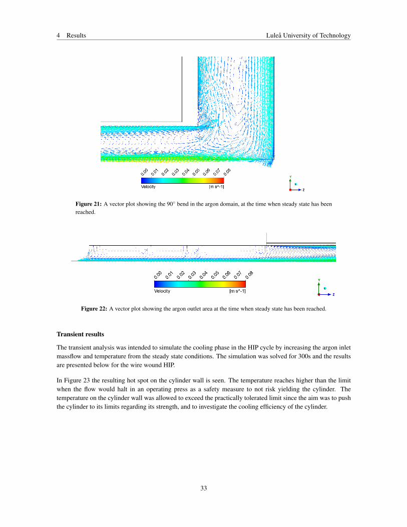
4 Results Luleå University of Technology
Figure 21: A vector plot showing the 90◦ bend in the argon domain, at the time when steady state has beenreached.
Figure 22: A vector plot showing the argon outlet area at the time when steady state has been reached.
Transient results
The transient analysis was intended to simulate the cooling phase in the HIP cycle by increasing the argon inletmassflow and temperature from the steady state conditions. The simulation was solved for 300s and the resultsare presented below for the wire wound HIP.
In Figure 23 the resulting hot spot on the cylinder wall is seen. The temperature reaches higher than the limitwhen the flow would halt in an operating press as a safety measure to not risk yielding the cylinder. Thetemperature on the cylinder wall was allowed to exceed the practically tolerated limit since the aim was to pushthe cylinder to its limits regarding its strength, and to investigate the cooling efficiency of the cylinder.
33
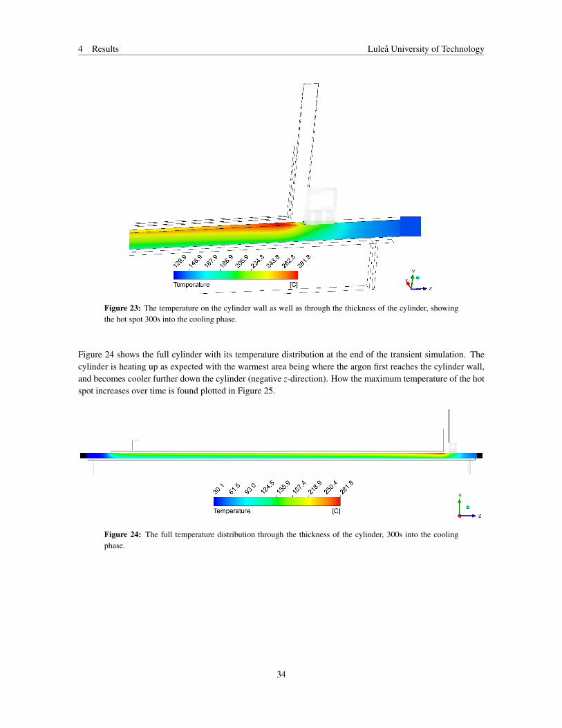
4 Results Luleå University of Technology
Figure 23: The temperature on the cylinder wall as well as through the thickness of the cylinder, showingthe hot spot 300s into the cooling phase.
Figure 24 shows the full cylinder with its temperature distribution at the end of the transient simulation. Thecylinder is heating up as expected with the warmest area being where the argon first reaches the cylinder wall,and becomes cooler further down the cylinder (negative z-direction). How the maximum temperature of the hotspot increases over time is found plotted in Figure 25.
Figure 24: The full temperature distribution through the thickness of the cylinder, 300s into the coolingphase.
34
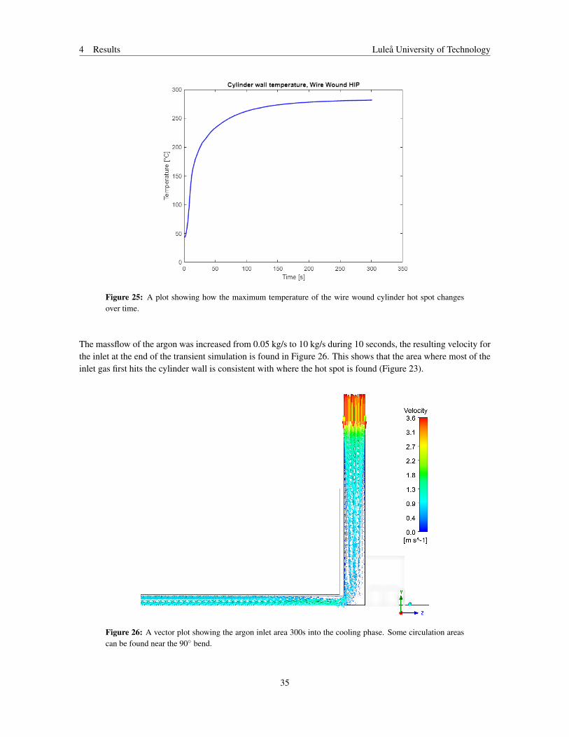
4 Results Luleå University of Technology
Figure 25: A plot showing how the maximum temperature of the wire wound cylinder hot spot changesover time.
The massflow of the argon was increased from 0.05 kg/s to 10 kg/s during 10 seconds, the resulting velocity forthe inlet at the end of the transient simulation is found in Figure 26. This shows that the area where most of theinlet gas first hits the cylinder wall is consistent with where the hot spot is found (Figure 23).
Figure 26: A vector plot showing the argon inlet area 300s into the cooling phase. Some circulation areascan be found near the 90◦ bend.
35

4 Results Luleå University of Technology
Moreover, the water in the cooling channel was heated by the cylinder as expected and the outlet temperaturewas higher than the 30◦C inlet. In Figure 27, the water domain is shown at the end time of the simulation. It canappear as though the temperature increase is very high based on the range of the scale, but it should be notedthat the highest temperatures are only found closest to the cylinder interface (with the peak of 146◦C beingclosest to the hot spot). This is however likely to be caused by numerical boundary effects, as no such hightemperatures has been observed. Figure 28 shows the water outlet and how the temperature varies dependingon the distance to the cylinder.
The temperature difference between the outlet and inlet of the water channel is 22◦C if measuring using areaaveraged values. However, the 2D model comes with some implications as the solid cooling rods are excludedfrom the model, thus the flow velocity of the water becomes lower than the true value. There was an attempt toevaluate different variations of the water channel model, this is shown and discussed further in section A.
Figure 27: The temperature of the water with the inlet being to the left and outlet to the right in the domain.The high temperature seen in the scale is found by the cylinder interface, at the area where the cylinder isthe warmest.
Figure 28: A close up of the water outlet, showing how the water is heated near the cylinder interface.
36
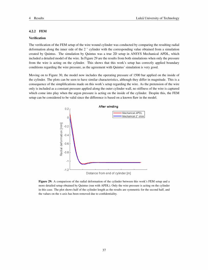
4 Results Luleå University of Technology
4.2.2 FEM
Verification
The verification of the FEM setup of the wire wound cylinder was conducted by comparing the resulting radialdeformation along the inner side of the 2 ◦ cylinder with the corresponding value obtained from a simulationcreated by Quintus. The simulation by Quintus was a true 2D setup in ANSYS Mechanical APDL, whichincluded a detailed model of the wire. In Figure 29 are the results from both simulations when only the pressurefrom the wire is acting on the cylinder. This shows that this work’s setup has correctly applied boundaryconditions regarding the wire pressure, as the agreement with Quintus’ simulation is very good.
Moving on to Figure 30, the model now includes the operating pressure of 1500 bar applied on the inside ofthe cylinder. The plots can be seen to have similar characteristics, although they differ in magnitude. This is aconsequence of the simplifications made on this work’s setup regarding the wire. As the pretension of the wireonly is included as a constant pressure applied along the outer cylinder wall, no stiffness of the wire is capturedwhich come into play when the argon pressure is acting on the inside of the cylinder. Despite this, the FEMsetup can be considered to be valid since the difference is based on a known flaw in the model.
Figure 29: A comparison of the radial deformation of the cylinder between this work’s FEM setup and amore detailed setup obtained by Quintus (run with APDL). Only the wire pressure is acting on the cylinderin this case. The plot shows half of the cylinder length as the results are symmetric for the second half, andthe values on the x-axis has been removed due to confidentiality.
37

4 Results Luleå University of Technology
Figure 30: A comparison of the radial deformation of the cylinder between this work’s FEM setup and amore detailed setup obtained by Quintus (run with APDL). Both the wire and argon pressure is acting on thecylinder in this case. The plot shows half of the cylinder length as the results are symmetric for the secondhalf, and the values on the x-axis has been removed due to confidentiality.
Mesh independence study
A mesh study was conducted for the FEM model of the wire wound cylinder in order to investigate the reliabilityof the results with respect to the mesh size. For all models a mesh element size of 4 mm was chosen. In Figure31 is a comparison of the resulting maximum principal stress in the cylinder for four element sizes. It can beseen that the stresses differ somewhat for the coarser meshes, while the 1.5 mm grid can be considered to bemesh independent.
38

4 Results Luleå University of Technology
Figure 31: Plots of the resulting maximum principal stress in the cylinder over time, for different meshsizes.
Further comparisons can be found in Figure 32, where the maximum values in Figure 31 are plotted againstthe number of elements in each respective mesh. The red star in the plot indicates the mesh of 4 mm whichwas used in the final FEM models. One can conclude that the maximum value of the principal stress for the 4mm mesh differs 0.4% from the corresponding value of the finest mesh. As the difference between these plotsare seemingly the same also after the peak in Figure 31, the difference will not increase much more than 0.4%.Therefore the 4 mm mesh is confirmed to provide adequate results as the difference is < 1% from a completelymesh independent result.
39

4 Results Luleå University of Technology
Figure 32: The maximum value found in the plots in Figure 31, plotted against the number of elements ineach mesh. The red star indicates the mesh that was used when producing the final results.
FEM Results
The results of the FEM analyses of the wire wound cylinder showed a deformation corresponding well with theapplied loads. In Figure 33, the von-Mises stress of the full cylinder is seen at the end stage of the simulation.The mechanical loads acting on the inside and outside of the cylinder are the gas pressure of 1500 bar and thewire pressure of 1820 bar. Since the wire pressure is applied on a surface reaching further along the outside ofthe cylinder than the gas pressure reaches on the inside, bending occurs as can be seen at the ends of the cylinder.At the same time, the thermal load is causing the cylinder to deform outwards due to thermal expansion, as theinside of the cylinder is warmer than the outside.
Figure 33: Von-Mises stress in the whole cylinder after 300s, with the loads applied being the temperatureload from CFX as well as pressure loads on the inside and outside of the cylinder representing the argonand wire pressure of 1500 bar and 1820 bar respectively. The deformation is scaled by a factor of 20 in thefigure.
Figure 34 shows close-ups of the top part of the cylinder in the beginning (2s) and end (300s) of the simulation.In the beginning, the thermal load is relatively low and thus the mechanical loads are causing most of the
40

4 Results Luleå University of Technology
deformation, with the wire pressure being predominant. As the temperature increases, mainly on the inside wall,the thermal expansion is acting with the gas pressure and relieves the bending - thus lowering the maximumvon-Mises stress. This implies that the mechanical loads give rise to the highest stresses when the thermal loadis low.
(a) Von-Mises stress at the first temperature load step (2s). (b) Von-Mises stress at the last temperature load step (300s).
Figure 34: A comparison of the von-Mises stress in the top part of the cylinder at the beginning versus theend of the structural simulation. What differs between them is the temperature load, which is low in thebeginning and has reached its peak by the end.
From the same figure it seems as though the cylinder is at risk of yielding at the ends where the bending occurs.However, in reality, the areas on which the pressures are acting are not abruptly cut off as they are in the FEMmodel. Because of this, there might be an exaggeration of the stresses caused by the mechanical loading. Inorder to easier be able to conclude the magnitude of the stresses caused by the thermal load, the cylinder ends(where the maximum stresses are found) were cut off from the results. The area with the maximum von-Misesstress could then be seen to coincide with the temperature hot spot. When plotted over time the peak of themaximum thermal stress is seen to occur before the temperature on the wall has reached its maximum (seeFigure 35 and 25). This can be explained by relating the stress to the temperature gradient through the cylinderwall which is the largest at the time of the stress peak. As the heat distributes more evenly through the cylinder,and the gradient levels out, the maximum thermal stress is consequently lowered because of relaxation.
41

4 Results Luleå University of Technology
Figure 35: The von-Mises stresses of the wire wound cylinder with the end parts of the cylinder excludedin order to capture the impact of the thermal load.
Even though the HIP model had a high argon inlet massflow, and the temperature on the cylinder wall exceededthe practically tolerated value, the thermal loading on the cylinder does not seem to cause any immediate riskof yielding. Although, in order to keep a safety margin it would not be recommended to run the HIP with suchconditions without having an additional cooling configuration installed.
Lastly, the normal stress of the cylinder was analysed with respect to the tangential direction of the cylindricalcoordinate system. This was to see if the cylinder was subjected to tensile or compressive stresses. The result isfound in Figure 36 and shows that the whole cylinder is subjected to compressive stresses, which is consistentwith real observations.
Figure 36: Normal stress of the cylinder with respect to the cylindrical tangential axis.
4.3 Monoblock HIP
Following the wire wound HIP model is the corresponding monoblock version. The geometry of the argongas and adjacent parts are equal to the wire wound version. The cylinder however is roughly 7 times as thick.Presented below are the results of the first case of monoblock HIP models. Meaning that on the outside of thecylinder is a water cooling channel, this has the same dimensions and flow conditions as the one found in the
42

4 Results Luleå University of Technology
wire wound model. For a presentation of the results for case 2, where the cylinder is cooled by solid coolingrods on the outside, see appendix B.
4.3.1 CFD
In this part, the steady state and transient results are presented of the monoblock CFX simulations. These resultsare to be compared with the ones on the wire wound HIP presented in the previous section, and the comparisoncan be read in the upcoming section 4.4.
Steady state results
The temperature distribution through all domains when steady state has been reached is seen in Figure 37. Aswas the case with the wire wound HIP, the flow of the gas is mainly driven by natural convection and hence theflow pattern and velocities are roughly the same as those seen in Figures 20 to 22.
Figure 37: The temperature throughout all domains of the monoblock HIP, at the time when steady statehas been reached. The inlet temperature of the argon gas is 100◦C, and the inlet temperature of the watercooling on the outside of the cylinder is 30◦C.
Transient results
After running the transient simulation of the monoblock HIP model, the hot spot on the cylinder wall reachedjust above 300◦C, see Figure 38. Figure 39 shows the temperature of the whole cylinder, and Figure 40 presentsthe maximum temperature of the cylinder plotted against time.
43

4 Results Luleå University of Technology
Figure 38: The temperature on the cylinder wall as well as through the thickness of the monoblock cylinder,showing the hot spot 300s into the cooling phase.
Figure 39: The full temperature distribution through the thickness of the monoblock cylinder, 300s into thecooling phase.
44

4 Results Luleå University of Technology
Figure 40: A plot showing how the maximum temperature of the monoblock cylinder hot spot changes overtime.
The temperatures of the water domain is found in Figure 41. In the scale are some higher temperatures that arenot seen in the plot, these are located along the cylinder interface. See Figure 42 for a close up of the waterchannel outlet and how the temperature is depending on the distance from the cylinder. The temperatures in thewater channel indicate that only a very small amount of heat is transported away from the cylinder through thewater.
Figure 41: The temperature of the water with the inlet being to the left and outlet to the right in the domain.The highest temperatures in the scale are found near the cylinder interface.
45

4 Results Luleå University of Technology
Figure 42: A close up of the water outlet, showing how the water is heated near the cylinder interface
4.3.2 FEM
From the FEM analyses of the monoblock cylinder, a few observations were made. First of all, despite exceedingthe temperature limit on the cylinder wall by roughly twice the value of the wire wound version, the cylinder isnot close to yielding according to the maximum von-Mises stress seen in Figure 43.
Secondly, the deformation of the cylinder is depending on the thermal load in a way that causes the cylinder toexpand inwards. See Figure 44 for a comparison of the von-Mises stress in the top part of the cylinder at boththe beginning (2s) and end (300s) of the simulation. In the beginning, the gas pressure on the inside is causingthe cylinder to expand outwards. But as the cylinder heats up on the inside, while a large fraction of the materialon the outer part remains relatively cold, the thermal expansion of the material is acting inwards (as opposed toacting with the pressure and expand outwards). This is believed to be due to the large part of the cylinder beingcolder (see Figure 39) and thus counteracting the expansion.
46

4 Results Luleå University of Technology
Figure 43: Von-Mises stress in the whole monoblock cylinder after 300s, with the loads applied being thetemperature load from CFX as well as a 1500 bar pressure load on the inside of the cylinder representing theargon pressure. The deformation is scaled by a factor of 200 in the figure.
(a) Von-Mises stress at the first temperature load step (2s). (b) Von-Mises stress at the last temperature load step (300s).
Figure 44: A comparison of the von-Mises stress in the top part of the cylinder at the beginning versus theend of the structural simulation. What differs between them is the temperature load, which is low in thebeginning and has reached its peak by the end.
The maximum and average values of the von-Mises stress in the monoblock cylinder is seen plotted in Figure45. In the first < 50s, the maximum stress first decreases to then start increasing. This has to do with theunevenness of the temperature load; while the temperature further down the cylinder remains fairly constant thetemperature at the top increases more rapidly. Initially, the maximum stress is found further down the cylinderand is caused by the mechanical load. What happens is that the thermal load in this area causes relaxation ofthe stress, and as the top part heats up the maximum stress arises there instead, increasing with the temperature.
47

4 Results Luleå University of Technology
Figure 45: The average and maximum von-Mises stresses of the monoblock cylinder plotted over time.
Regarding the normal stress throughout the cylinder, evaluated along the cylindrical tangential axis, the resultsshow that the cylinder is subjected to compressive stresses on the inside where the temperature load has itsmaximum, and that the stresses then transition to tensile when moving through and down the cylinder. This canbe seen in Figure 46.
Figure 46: Normal stress of the cylinder with respect to the cylindrical tangential axis.
4.4 Results comparison
Comparing the results of the wire wound HIP model with the monoblock version reveals some differences inthe heat transfer efficiencies and structural capabilities. Below is a summary of how these cylinders measureagainst each other in these areas.
48

4 Results Luleå University of Technology
4.4.1 CFD
Considering the size of the monoblock cylinder compared with the cylinder found in the wire wound model, itis only logical that the monoblock has a higher heat storage capacity and should thus become warmer duringthe holding stage. Comparing the results from the steady state analyses it can be seen that the maximumtemperature of the monoblock cylinder is roughly 11◦C warmer than the corresponding temperature of the wirewound cylinder, see Figure 47.
(a) Wire wound cylinder
(b) Monoblock cylinder
Figure 47: The temperature distributions for the different cylinders when steady state has been reached.The monoblock cylinder is seen to be somewhat warmer than the wire wound version.
Other than the difference in temperature of the two cylinders, the steady state results showed no significantvariations. Moving on to the transient analyses, the differences became more clear. The heat flow rate from theargon to the cylinder, and from the cylinder to the water channel, is plotted in Figures 48 and 49 respectively.Regarding the heat flow from the argon to the cylinder, the rates do not differ much in the first 10s when themassflow of the gas is increasing and the temperature is reaching 400◦C. As the gas has reached 400◦C, thetemperature difference between the gas and cylinder wall is the highest, thus the heat flow rate reaches itspeak due to the law of forced convection [25]. After this, the cylinder walls are heating up and reduces thetemperature difference, making the heat flow rate decrease for both cylinder versions. The heat flow rate of thewire wound model can be seen to level out after some time, while the monoblock plot continues to decrease asits large thermal mass causes the cylinder wall to reach a higher temperature, and thereby lower the heat flowrate.
The fact that the monoblock cylinder’s cooling rate is decreasing can be explained by its large heat storagecapacity. As the cylinder heats up the temperature difference between the gas and cylinder decreases, whichmakes the cooling rate caused by forced convection slow down [25]. As seen in Figure 49, the amount of heattransferred to the water is very low in comparison with the wire wound model. The plot in the figure can seemto be level, but it is in fact decreasing, thus confirming the fact that no steady state has been reached.
49

4 Results Luleå University of Technology
Figure 48: A comparison of the heat flow from the argon gas to the cylinder at each time step for bothcylinder versions analysed.
Figure 49: A comparison of the heat flow from the cylinder to the water at each time step for both cylinderversions analysed. The plot is showing negative values since the calculations are based on the cylindersurface which is giving off heat to the water.
A summary of the results from the transient CFD analyses of both cylinder versions is found in Table 7. Thetemperatures are measured using an area averaged value of the corresponding inlets/outlets, and the total heatlosses are calculated by integrating the CFX results plotted in Figures 48 and 49.
50

4 Results Luleå University of Technology
Table 7: A comparison of some numerical results between the two cylinder versions analysed.
Wire Wound Monoblock Difference [%]Argon outlet temperature [◦C] 327 338 3.4∆TArgon [◦C] 73 62 18∆TWater [◦C] 22 0.90 2300Total heat loss Argon→ Cylinder [kW] 498 464 7.3Total heat loss Cylinder→Water [kW] -334 -15.1 2100Maximum temperature cylinder wall [◦C] 282 301 6.7
Although it seems as though there is not a large difference in the cooling rate between the wire wound andmonoblock cylinder, one should keep in mind that the monoblock has not reached a steady state in the 300simulated seconds. Therefore, if the simulation would be run for longer, the difference in their cooling efficiencieswould become more apparent.
Apart from the plot of the heat flow rate in Figure 49, the inefficiency of the cooling water to transport awayheat from the monoblock cylinder can also be confirmed by the results in Table 7. There is a clear differencebetween the temperature increase of the water between the cylinders, and the amount of heat transferred awayby the water is around 70% of what is taken from the argon for the wire wound cylinder, while the correspondingfigure is 3% for the monoblock cylinder. This correlates with the monoblock cylinder’s high thermal mass.
4.4.2 FEM
The results of the FEM analyses show that neither one of the cylinders are at immediate risk of yielding at thecurrent thermal loads, which are higher than the load allowed in an operating wire wound HIP. The wire woundcylinder is though more close to yielding than the monoblock as the maximum von-Mises stress caused by thethermal load is higher. Hence the wire wound HIP should have a more strict hot spot temperature limit than themonoblock HIP.
There is indeed a difference in the characteristics of the plots showing the maximum von-Mises stress in Figures35 and 45. The stress in the wire wound cylinder reaches a peak value and then decreases to a steady state,while in the monoblock cylinder the stress is increasing towards a steady state. This difference is caused by thedifference in the geometry and mechanical loadings. The wire wound cylinder experiences the highest stress inthe beginning when the cylinder has its peak temperature gradient through the thickness of the material. As thegradient decreases and the hot spot becomes warmer, the thermal load acts by expanding the cylinder outwardsand thus reduces the stress caused by the outer wire pressure. The monoblock cylinder on the other hand hasa correlation between increased temperature and increased stress. As the only mechanical load is the inner gaspressure, and the thermal load causes an expansion inwards, the loads work against each other and causes anincrease in stress.
Furthermore, the results confirm the known difference about the cylinders: the wire wound is experiencingcompressive stresses throughout the whole cylinder, while the monoblock cylinder mainly is in a tensile stressstate (apart from around the hot spot where the thermal expansion is highly local and thus gives rise to compressivestresses).
The fatigue life of the wire in all of Quintus’ HIPs is computed to ensure a safe construction. For the wire inthe HIPs analysed in this work, the fatigue life is more than 20 000 cycles. It should be noted though that thewire in practice can withstand many more cycles, since even though the wire fractures in multiple places, it can
51

4 Results Luleå University of Technology
still hold the pretension. The cylinder however is capable of withstanding over 200 000 cycles according tocomputations performed by Quintus, following the ASME division 3 standard [26].
Since the monoblock cylinder did not risk yielding, a fatigue analysis was computed, following the ASMEdivision 2 standard [23]. This resulted in the cylinder withstanding just above 60 000 cycles when havingnormal operating flow conditions. When subjected to the more extreme inlet conditions, as described in Table4, the number of cycles was reduced to just under 17 000.
52

5 Discussion Luleå University of Technology
5 Discussion
In this chapter, the methodology and results of the validation study, followed by the CFD and FEM models ofthe HIPs, are discussed.
5.1 Validation study
As can be seen in the results of the validation study (Table 5) there is a deviation regarding the pressure drop inthe annular pipe, when compared to the experimental data. The same applies to the Fanning friction factor, C f ,since this is dependent on the pressure drop of the inner pipe, which in turn also differs from the experimentalone.
These deviations found in the numerical results of the pressure drop can first of all be caused by uncertaintiesregarding the mounting of the sensors in the experimental setup. In [9], it is said that the pressure andtemperature sensors were mounted at a location of 10 D from the inlets and outlets, i.e. a distance of 0.22m. However, in the report describing the experimental setup in detail, [27], it can be seen that the sensors arenot mounted with such high accuracy since there is a distance between the pressure and temperature sensor ateach measurement location.
Secondly, the DPHx was modelled without the solid inner pipe included. This in order to reduce computationalrequirements and because it appeared as this was the approach taken for the numerical model in [9]. Instead, aninterface between the fluid domains was defined with a ”thin material” covering the interface. This resulted inthe water of the annular side having a larger volume than in reality because of the lack of physical thickness ofthe inner tube, which in turn would have an effect on the pressure drop.
There is also an uncertainty regarding the geometry where the hot water pipe expands/contracts and does a 90◦
turn. It is not defined if the expansion/contraction in the experimental setup is sharp, which it is in the numericalmodel, or if there is some transition radius. Since these geometrical differences have a large effect on the losscoefficient, which in turn affects the pressure drop, this becomes a possible source of error to the pressure dropdeviations.
An attempt was made to measure the temperatures and pressures at the ends of the computational domain, i.e. atthe exact position of inlets/outlets of the DPHx. This produced results that were more close to the experimentalresults than the ones obtained at the, allegedly, same position as the sensors. It remains unknown if this is acoincidence, or if this position in fact is closer to the experimental sensor placements.
The mesh resolution was ruled out as a source of error since a finer mesh was also implemented, with 20·106
elements (same as the second grid described in [9]), but no prominent differences could be seen in the results.
Regardless of the uncertainty of measurement locations, the numerical model was able to capture the heattransfer, Q, in an accurate way when compared to the experimental results. This is the result of most importancesince this will be analysed in the HIP. Thus the RANS turbulence models have been confirmed to be anappropriate method for capturing the types of physics of interest in a truthful way.
5.2 CFD
In this section are some reflections on the methodology and results regarding the CFD models of both the wirewound and monoblock models.
53

5 Discussion Luleå University of Technology
5.2.1 Methodology
Modelling approaches of cooling channel
Because of the limited resources regarding computational power, all models of the HIP was created as a 2Daxisymmetric representation of the full geometry. This was a delimiting factor when modelling the water coolingchannel as the construction of this, with its vertical solid rods and water flowing in the channels between them,is not possible to capture accurately in a 2D model.
In the methodology and results presented in this report, the water cooling channel was modelled by simplydisregarding the solid cooling rods and considering the whole domain as fluid water, without changing itsthickness. By doing so, the conductive heat transfer through the rods was eliminated and the flow speed ofthe water got lower than the speed in an operating HIP. Thus the cooling capacity of the water channel wasunderestimated. This might have caused the wire wound cylinder to appear as less effective in its cooling ratethan what would be the case in reality. Since the monoblock cylinder proved to not transport away much heatwith the water during the first 300s of the cooling phase, a more true representation of the water channel wouldnot affect that result noteworthy. Meanwhile, the cooling rate of the wire wound cylinder was highly dependenton the water channel, and the cooling capacity of this cylinder is thus likely to be underestimated.
Initially, two additional versions of water cooling channels was modelled with the intention of evaluating thedifference between them. The first version had an adjusted thickness of the channel, 1/4 times the thickness ofthe original, which produced a total volume of water corresponding to the volume in a real HIP. Thus the flowspeed of the water got closer to the correct value, but still no conduction was included. The second versionallowed conduction by modelling the water as a solid with its thermodynamic properties defined as the meanvalue between water and steel, based on the ratio between them.
The additional water channel models were not evaluated thoroughly due to the long simulation times whichcaused the study to be put aside in order to stay within the planned time frame. The models and some simplesteady state CFD results can be found in appendix A. What could be concluded from the steady state resultswas that the choice of modelling approach of the water channel does indeed have an impact on the possibleheat transfer from the wire wound cylinder to the water. Hence the water channel modelling is of interest toinvestigate further, and the differences give rise to additional interest in constructing a 3D model of the HIP.
Steady state convergence issues
There were some difficulties with achieving converged steady state solutions, mainly regarding the RMS residuals.Instead of dropping to the target of 1e-5, the residuals leveled out and showed an oscillating behaviour, with thehighest one oscillating around 1e-3. At this stage the geometry of the argon outlet was modelled according toFigure 50.
When analysing the results, the outlet area in the argon domain showed a large recirculation pattern whichcaused a high amount of backflow. This was found to be the main cause of the high residuals, and did notimprove by defining the outlet as an opening.
An attempt was made to extend the outlet further to avoid the recirculation area, but with little improvement ofthe convergence. The timescale factor was also altered during the course of the solution, with a higher time stepin the beginning in order to avoid any possible transient phenomenons. Neither this, or changing the advectionscheme to upwind, had a significant impact on the convergence. A slight improvement could be obtained whenusing a physical timescale with a low time step size. However, this came with the cost of very high simulationtimes and was thus not considered to be a convenient alternation.
54

5 Discussion Luleå University of Technology
Figure 50: The original geometry of the outlet area in the argon domain, with the outlet surface being theone marked in orange. This large chamber gave rise to high residuals due to a large recirculation area.
The solution to the convergence problem came to be an alternation of the outlet geometry. The large outletchamber was removed and the channel was instead extended as far as the argon was in contact with the cylinderin the real HIP (see the final geometry in, for example, Figure 9). This alternation did however result in a lesstrue representation of the outlet. But since the flow in the outlet area was not a crucial part to capture, the resultsin focus were deemed to be unaffected.
Mesh independence
The mesh independence study was only conducted on the wire wound HIP and not the monoblock. Since theargon and water domains are of the same dimensions and flow conditions for both models, it should be sufficientwith this one study. However, in order to fully establish mesh independent results, some more values would bebeneficial to compare against the different mesh sizes.
The mesh study was done with a limited time frame, hence the study would be possible to extend further.Previous CFD analyses of HIPs performed by Quintus have though used a similar fluid bulk mesh size, thus themesh size is considered to be reasonable. Although, if the work were to be recreated, a coarser mesh would bebeneficial to use initially, until the setup had been calibrated satisfactory. This is because of the long simulationtimes of the transient runs, which could vary from 4h for the smaller HIP, and up to 4 days for the larger version.
5.2.2 Results
The CFD model of the wire wound HIP was simplified by not including the load area, inner mantle or top/bottomclosures. The inlet flow conditions were based on measurements from an operating HIP of the same size,measured around the area of the CFD model’s inlet. These simplifications were considered to be justified as
55

5 Discussion Luleå University of Technology
the full gas flow path should not be necessary to capture for this type of comparative analysis, as long as allboundary conditions are correct and equal.
Despite this, the resulting temperature on the cylinder wall in the wire wound CFD simulation was expected tobe somewhat close to measured values, for when the CFD setup included normal gas inlet conditions. Thetemperature was however lower than what had been measured in an operating HIP. The CFD simulationstherefore seem to have a tendency of underestimating the heat transfer between the argon gas and cylinder.This could be a consequence of poor capturing of the turbulence in the argon gas. To investigate this further,one could conduct a closer study of the boundary layer resolution and y+-value for the fluid domains, as thiswas not checked thoroughly due to time limitations.
Another indication that the CFD models might underestimate the heat transfer is the steady state result of themonoblock simulation. Because of the monoblock cylinder’s high thermal mass, it should have the capacity ofreaching a considerably higher temperature than the wire wound cylinder during the holding phase of the HIPprocess. In parallel with the thesis work, a CFD simulation created by Quintus was run to check the differencein steady state temperatures of the cylinders. This model included the inner parts of the HIP in more detail, withthe heaters and full gas path captured. When running a monoblock version of this setup, the steady state resultsshowed a temperature difference between the wire wound and monoblock cylinder around double the value ofwhat was obtained in this work’s setup.
An error source found in both this work’s model, and the one created by Quintus, is the modelling of the innermantle’s material. In this thesis it is modelled as a solid, while it in reality has a porous structure. Thus themantle has some heat leakage due to this porosity, which the CFD models are unable to capture. There mighttherefore be some heat transfer to the argon that is missing.
The plots of the heat flow rate between the argon and cylinder in Figure 48 show that the rates do not differmuch in the beginning of the cooling. This is related to the low difference in temperature between the cylinderversions. However, if the steady state analyses indeed do result in an underestimated temperature on the cylinderwall, the cooling rate of the monoblock cylinder is likely to be overestimated in the beginning of the transientsimulation. This is because the heat flow rate is a function of the temperature difference between the argonand cylinder wall when considering forced convection [25], which would decrease the heat flow rate if themonoblock cylinder were to be warmer at the beginning of the cooling. As time increases, the heat flow rate inthe wire wound model levels out after the peak, while the rate in the monoblock version continues to decreaseas the temperature on the cylinder wall has not yet reached a steady value. This indicates that the monoblockcylinder can not quite measure with the wire wound regarding the cooling rate. This is especially true towardsthe end of the cooling stage according to the results of this thesis work, hence the monoblock HIP might beunfavourable to the wire wound, if one wish to cool down the gas to lower temperatures.
5.3 FEM
In this section are some reflections on the methodology and results regarding the FEM models of both the wirewound and monoblock models.
5.3.1 Methodology
Regarding the method when constructing the FEM model of the cylinders, some simplifications and assumptionswere made. First of all, a pressure was applied along the outside of the wire wound cylinder wall in order torepresent the pressure acting on the cylinder from the pretension of the wire. This pressure was applied asconstant both with respect to time and axial distance of the cylinder. While in reality, the pressure varies with
56

5 Discussion Luleå University of Technology
both the time and distance. This simplification was made due to the time limitations of the project, but wasalso considered to be justified as it eased the interpretation of the thermal stresses, which were of the greatestinterest to analyse. An assumption was also made regarding the argon pressure, which was set to 1500 bar. Thispressure can vary between different HIPs and cooling cycles, but it was considered to be an appropriate generalpressure when initiating the cooling stage.
A mesh study was conducted for the wire wound cylinder, which showed that an even coarser mesh would bejustified to use. However, the simulation times of the FEM analyses with the finer mesh that was used stayedaround∼15min, which was not an inconvenient time and hence a coarser mesh would not be very advantageous.
5.3.2 Results
The validation study of the FEM analysis confirm the known fact that the wire simplification has some impacton the results. Figure 30 imply that the radial deformation of the cylinder is overestimated in this work’s setup,at the point of its maximum deformation (referring to absolute values). Since the maximum von-Mises stressis found in the area of the maximum deformation (seen in Figure 34), the cylinder should in reality not besubjected to such high stresses. This was though taken into account when analysing the von-Mises stress of thewire wound cylinder, as the end parts where the maximum deformation occured was excluded in order to moreclearly see the impact of the thermal load.
Regarding the monoblock cylinder, a more clear relation could be seen directly between the thermal load andthe von-Mises stress, since the maximum stress was found around the temperature hot spot. The deformationof the monoblock cylinder was an interesting observation since it was expected that the thermal load wouldcause the whole cylinder to expand outwards, but with a large part of the cylinder being colder the expansionwas acting more locally and thus causing an expansion inwards. This is though with the high inlet massflow(multitudes larger than normal for a HIP of this size) and the cylinder wall thereby reached a higher temperaturethan what would be observed with normal inlet conditions. It would hence be of interest to investigate the wirewound/monoblock comparison using normal inlet flow conditions.
The fatigue analysis of the monoblock cylinder showed that the cylinder can withstand a satisfactory number ofcycles when operating with normal inlet flow conditions. But when the inlet massflow corresponded to that ofa URQ unit, the number of cycles reduced below 20 000, which the wire wound HIP is capable to withstand. Itshould be noted that, as mentioned in section 4.4.2, the cylinder itself in the wire wound HIP can withstand over200 000 cycles, and that the wire is the limiting facor with respect to fatigue life. In that sense, the monoblockcylinder does not measure with the wire wound.
It is of great importance to have a clear understanding of the stresses acting on the monoblock cylinder sincea failure of this cylinder could have catastrophic consequences. The FEM simulations in this work confirmthat the monoblock cylinder is mostly subjected to tensile stresses, especially on the outside. Thus if a crackis initiated it will propagate and could result in an explosive failure. The fatigue analyses showed that themonoblock cylinder is indeed capable of withstanding >20 000 cycles, the number of cycles is however highlydepending on the thermal load acting on the cylinder together with the argon pressure. This places high demandson properly designed monoblock cylinders.
5.4 General
Initially, the steady state CFD setup was not believed to be vital to model correctly to 100% as the transientresults were those of greatest interest. As it turned out, the steady state results did affect the transient resultsby influencing the initial cooling rate of the gas since the different cylinders were expected to differ more in
57

5 Discussion Luleå University of Technology
temperature. More time could therefore have been spent assuring that the steady state boundary conditions andresults were plausible.
The idea in the beginning of this thesis work was that by allowing the temperature on the cylinder walls exceedthe maximum allowed value, the cylinders would risk yielding. This did not occur for either the wire woundor monoblock cylinder, even though the inlet massflow rate was increased many times higher than the normaloperating value. Because of this, the interpretation of the results had to be reconsidered. The thought was tocompare how much heat each cylinder could transfer away until it began to yield, but this was then altered tosimply comparing the cooling rates and total heat losses, together with the fatigue analysis of the monoblockcylinder.
Since neither of the cylinders did yield, the work could have been conducted with normal inlet flow conditionsto get more true absolute results. Although, it is still the relative results which are of the highest interest, hencethe increased massflow rate does not make the results invalid. Another approach the work could have takenwould be to work in an iterative way and increase the inlet massflow until the cylinder would yield. This wouldhowever require massflows that are not realistic to use in an operating HIP, thus creating irrelevant results.Because of the long simulation times and high number of different models, that kind of work approach wouldalso be too time demanding to apply.
In this project the inlet temperature of the argon gas remained constant. In reality the temperature reaching thecylinder vary over time as the gas travels in a closed loop and continuously cools down. This means that for themonoblock cylinder, the inlet gas temperature would decrease more slowly than in the wire wound case becauseof the difference in cooling capabilities. The results obtained in this work is sufficient for comparison purposesas mentioned earlier. But for a more clear difference between the two constructions, the full gas loop wouldhave to be modelled.
To conclude the general notes, this master’s thesis work has provided a lot of new, and somewhat unexpected,insights into how a monoblock HIP construction would measure against Quintus’ wire wound HIPs. The resultsshowed that the monoblock cylinder can indeed measure with the wire wound in terms of fatigue life, but not asmuch when it comes to cooling rate. This is knowledge that is of interest to Quintus, as it gives them a deeperunderstanding of the field of hot isostatic pressing. In addition, a foundation has been laid for them to conductfurther investigations of the monoblock HIP.
58

6 Conclusions Luleå University of Technology
6 Conclusions
A summary of the major conclusions drawn from this thesis work are listed below.
• The validation study of the double pipe heat exchanger confirmed that the RANS turbulence modelsshould be sufficient to use with this work’s flow conditions. For the FEM analyses, a comparison wasmade with a simulation created by Quintus. This confirmed that the setup created was correct, apart fromthe lack of a detailed model of the wire which had some effect on the deformation of the cylinder whenin a pressurised state.
• The CFD steady state setup of a HIP is of importance to model correctly when the results are to be usedas initial conditions for a transient CFD simulation, where the cooling rate is of interest to analyse. Thisis due to the influence the temperature distribution of the HIP in the holding phase has on the cooling rate.
• Comparing the cooling efficiencies of the monoblock and wire wound cylinder, the monoblock has ahigher thermal mass due to its large size, and is thus capable of storing a high amount of heat. This makesits cooling rate lower than the wire wound, especially after some time when the gas has cooled off a bit.
The water channel on the outside of the monoblock cylinder does not aid much in the cooling during thebeginning of the cooling phase, since the highest temperatures are still concentrated around the hot spoton the inner part of the cylinder. In this work the cooling was simulated for 300 seconds, during this timeno high temperatures had yet reached the outside of the cylinder and thus the heat transfer to the waterwas roughly 20 times higher in the wire wound cylinder.
• Neither of the cylinder versions turned out to be at risk of yielding with the flow conditions used in thiswork, but the wire wound did experience a 60% higher von-Mises stress maximum than the monoblock,due to the thermal load. For both versions the critical points are located around the hot spot on the insideof the cylinder. One should also remember that the monoblock cylinder is subjected to tensile stresses,meaning that if a crack is initiated in an area with tensile stress, it can result in a catastrophic failure ifthe allowed cycles of the cylinder is not correctly adjusted. Both cylinders are safe to withstand >20 000cycles.
• Regarding the different cylinder’s pros and cons, the wire wound HIP is still a safer construction as thefailure mode is not catastrophic. It is also possible to reach a higher cooling rate with the wire woundcylinder because of its slim design, confirmed by this thesis work. The wire wound HIP is a moreexpensive construction, but thanks to its high cooling rate, the total cycle times can be lowered and thecustomer can process a larger amount of components in a shorter time, thus reducing the long time costs.The monoblock cylinder on the other hand is a cheaper construction but can not cool the load with thesame rate.
59
7 Future Work Luleå University of Technology
7 Future Work
If more time would be available, there are some parts that could have been investigated further. This includesa closer analysis of the boundary layer and y+-value, as this has not been confirmed to be sufficiently resolvedsince that the inlet gas massflow rate was increased. The resolution can be checked by plotting the eddy viscosityratio and see how this transitions within the inflation layers [28]. Since the inlet massflow rate of argon gas wasincreased from the normal rate, a closer investigation could also be conducted regarding the turbulence model,as the increase in flow rate made the CFD validation work on the heat exchanger less comparable to the HIPsetup.
With more time at hand, one could also perform a more thorough mesh independence study of both the CFDand FEM setups. This was conducted for the steady state, wire wound, CFD model, and for the wire woundFEM model. Some more studies and values are though still possible to investigate. One could also perform acloser study of the convergence criteria for the transient CFD simulations. A residual target of 1e-4 was set, butbeacuse of the long simulation times no stricter criteria was tested.
Some additional areas that would have been interesting to add to this thesis work are listed below, some ofwhich might also be of relevance for Quintus to follow up on.
• Redo the work with normal inlet flow conditions of the argon gas, to see how the differences between thecylinders are affected. A few models were run with this configuration for investigate purposes, but it wastoo time consuming to run all models over again.
• Evaluate the modeling of the cooling water channel more thoroughly, and establish how the differentmodels presented in appendix A compare against each other in a transient run. These different modelscan also be applied to the monoblock with water cooling.
• Run a monoblock model without any cooling applied to the cylinder. This would perhaps not be anallowed construction in reality, but would provide some reference on how effective the different coolingmethods are.
• Investigate the monoblock cylinder further with respect to its thermal mass. If a new cycle were to beginbefore thermal equilibrium had been reached, one could study how this would affect the cylinder in termsof cooling rate and induced stresses.
• Extend the CFD models of both the wire wound and monoblock version by including the full gas loopand heaters, and simulating the entire cooling phase. This would create a more realistic setup wherethe temperature of the gas would cool off as a result of each cylinder’s cooling capability. This wouldprovide an even deeper understanding of how these HIP models differ regarding their cooling rate, andby simulating the full cooling time it would become more clear how the monoblock cylinder performs atlower gas temperatures.
• Create a 3D version of the wire wound and monoblock model. This would give an understanding of anypotential implications of using a 2D model. By creating a 3D model, one could also include solid coolingrods in the water channel and thus get a more accurate cooling of the cylinder.
60

8 References Luleå University of Technology
8 References[1] Quintus Technologies. Our heritage [Internet]; c2021. Cited 2021-02-09. Available from:
https://quintustechnologies.com/company/.
[2] Quintus Technologies. The specialist in High Pressure Manufacturing Technology [Internet]; c2021.Cited 2021-02-09. Available from: https://quintustechnologies.com/company/.
[3] Bocanegra-Bernal MH. Hot Isostatic Pressing (HIP) technology and its applications to metals andceramics. Journal of Materials Science. 2004 Nov;39(21):6399–6420.
[4] Quintus Technologies. This is Hot Isostatic Pressing [Internet]; c2021. Cited 2021-02-09. Availablefrom: https://quintustechnologies.com/hot-isostatic-pressing/.
[5] Quintus Technologies; c2021. Cited 2021-02-09. Available from: https://quintustechnologies.com.
[6] Eklund A, Ahlfors M. Heat treatment of PM parts by Hot Isostatic Pressing. Metal Powder Report. 2018Feb;73(3):163–169. Available from: https://doi.org/10.1016/j.mprp.2018.01.001.
[7] Jansson U. Heat transfer and thermal stress in highly pressurized vessel [master’s thesis]. LinköpingUniversity; 2020.
[8] Sjerling H, Ramstedt N. Prediction of the Quenching Performance in a Hot Isostatic Press UsingConjugated Heat Transfer [master’s thesis]. Linköping University; 2018.
[9] Córcoles JI, et al. Numerical and experimental study of the heat transfer process in a double pipe heatexchanger with inner corrugated tubes. International Journal of Thermal Sciences. 2020 Dec;158.Available from: https://doi.org/10.1016/j.ijthermalsci.2020.106526.
[10] Tu J, Yeoh GH, Liu C. Computational Fluid Dynamics: A Practical Approach. 2nd ed. Elsevier; 2013.
[11] Anderson J, Degroote J, Degrez G, Dick E, Grundmann R, Vierendeels J. Computational Fluid DynamicsAn Introduction. 3rd ed. Springer; 2009.
[12] Engineering Library. Laminar and Turbulent Flow [Internet]; c2021. Cited 2021-04-20. Available from:https://engineeringlibrary.org/reference/laminar-and-turbulent-fluid-flow-doe-handbook.
[13] Blazek J. Computational Fluid Dynamics: Principles and Applications. 2nd ed. Elsevier; 2005.
[14] Leap Australia. TIPS & TRICKS: TURBULENCE PART 1 - INTRODUCTION TO TURBULENCEMODELLING [Internet]; 2012. Cited 2021-04-20. Available from:https://www.computationalfluiddynamics.com.au/turbulence-modelling/.
[15] Zhai ZJ, Zhang Z, Zhang W, Chen QY. Evaluation of Various Turbulence Models in Predicting Airflowand Turbulence in Enclosed Environments by CFD: Part 1—Summary of Prevalent Turbulence Models.HVAC&R Research. 2007 Nov;13(6):853–870. Available from:https://doi.org/10.1080/10789669.2007.10391459.
[16] Leap Australia. WHAT Y+ SHOULD I USE? PART 1 - UNDERSTANDING THE PHYSICS OFBOUNDARY LAYERS [Internet]; 2020. Cited 2021-04-28. Available from: https://www.computationalfluiddynamics.com.au/y-plus_part1_understanding-the-physics-of-boundary-layers/.
61

8 References Luleå University of Technology
[17] CFD Online. Dimensionless wall distance (y plus) [Internet]; 2014. Cited 2021-05-04. Available from:https://www.cfd-online.com/Wiki/Dimensionless_wall_distance_(y_plus).
[18] ANSYS, Inc. Buoyancy; 2020. CFX-Solver Modeling Guide.
[19] A Altabey W, Noori M, Wang L. Using ANSYS for Finite Element Analysis: A Tutorial for Engineers.vol. 1. Momentum Press; 2018.
[20] COMSOL. Fluid-Structure Interaction [Internet]; 2017. Cited 2021-03-03. Available from:https://www.comsol.com/multiphysics/fluid-structure-interaction.
[21] Ansys. Fluid-Structure Interaction [Internet]; c2021. Cited 2021-03-03. Available from:https://www.ansys.com/products/platform/multiphysics-simulation/fluid-structure-interaction.
[22] Euro Inox. Stainless Steel: Tables of Technical Properties;. Available from: https://www.worldstainless.org/Files/issf/non-image-files/PDF/Euro_Inox/Tables_TechnicalProperties_EN.pdf.
[23] ASME Boiler & Pressure Vessel Code Section VIII, Division 2. ISBN 978-0-7918-7288-8. TheAmerican Society of Mechanical Engineers; 2019.
[24] ANSYS, Inc. Mesh; 2020. Mechanical User’s Guide.
[25] Engineering ToolBox. Convective Heat Transfer [Internet]; 2003. Cited 2021-06-21. Available from:https://www.engineeringtoolbox.com/convective-heat-transfer-d_430.html.
[26] ASME Boiler & Pressure Vessel Code Section VIII, Division 3. ISBN 978-0-7918-7289-5. TheAmerican Society of Mechanical Engineers; 2019.
[27] Moya-Rico JD, et al. Characterization of a triple concentric-tube heat exchanger with corrugated tubesusing Artificial Neural Networks (ANN). Applied Thermal Engineering. 2019 Jan;147:1036–1046.Available from: https://doi.org/10.1016/j.applthermaleng.2018.10.136.
[28] Leap Australia. TURBULENCE PART 4 - REVIEWING HOW WELL YOU HAVE RESOLVED THEBOUNDARY LAYER [Internet]; 2013. Cited 2021-06-22. Available from:https://www.computationalfluiddynamics.com.au/tips-tricks-turbulence-part-4-reviewing-how-well-you-have-resolved-the-boundary-layer/.
62
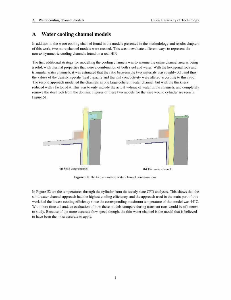
A Water cooling channel models Luleå University of Technology
A Water cooling channel models
In addition to the water cooling channel found in the models presented in the methodology and results chaptersof this work, two more channel models were created. This was to evaluate different ways to represent thenon-axisymmetric cooling channels found on a real HIP.
The first additional strategy for modelling the cooling channels was to assume the entire channel area as beinga solid, with thermal properties that were a combination of both steel and water. With the hexagonal rods andtriangular water channels, it was estimated that the ratio between the two materials was roughly 3:1, and thusthe values of the density, specific heat capacity and thermal conductivity were altered according to this ratio.The second approach modelled the channels as one large coherent water channel, but with the thicknessreduced with a factor of 4. This was to only include the actual volume of water in the channels, and completelyremove the steel rods from the domain. Figures of these two models for the wire wound cylinder are seen inFigure 51.
(a) Solid water channel. (b) Thin water channel.
Figure 51: The two alternative water channel configurations.
In Figure 52 are the temperatures through the cylinder from the steady state CFD analyses. This shows that thesolid water channel approach had the highest cooling efficiency, and the approach used in the main part of thiswork had the lowest cooling efficiency since the corresponding maximum temperature of that model was 44◦C.With more time at hand, an evaluation of how these models compare during transient runs would be of interestto study. Because of the more accurate flow speed though, the thin water channel is the model that is believedto have been the most accurate to apply.
i

A Water cooling channel models Luleå University of Technology
(a) Thin water channel.
(b) Solid water channel.
Figure 52: The temperature through the thickness of the cylinder in steady state, for the two additionalwater cooling channel models.
ii

B Monoblock Case 2 results Luleå University of Technology
B Monoblock Case 2 results
The second case of monoblock HIPs had no water to aid in the cooling of the cylinder. Instead, solid coolingrods were thought to be mounted on the outside of the cylinder. This was represented in the CFD setup byapplying a heat flux coefficient on the corresponding surface. Some results of the temperatures through thecylinder after the transient run are seen in Figures 53 and 54.
Figure 53: The full temperature distribution through the thickness of the monoblock cylinder, 300s into thecooling phase
Figure 54: The resulting temperature on the outside wall of the monoblock cylinder, where cooling rods arerepresented by a constant heat transfer coefficient.
In Figure 55 is a comparison of the cylinder temperature between Case 1 and 2, where the Case 2 result hasbeen subtracted from Case 1. This shows that the Case 1 cylinder is a few degrees warmer than the Case 2cylinder, especially in the lower part near the outer wall. This has mainly to do with the set temperature of thecooling water, which is 30◦C at the inlet, while in Case 2, the outside temperature is set to 20◦C. Towards themiddle of the cylinder the temperatures differ less, meaning that the heat transfer to the surroundings in Case 2is becoming less effective. This is confirmed in Table 8, where the heat loss to the surroundings in Case 2 isseen to be lower than to the water in Case 1. The other results seen in the Table indicate that there is not asignificant difference between the two monoblock configurations. The heat loss from the gas to the cylinder isstill roughly the same, and so are the temperature measurements. In order to conclude this similarity withcertainty though, a longer simulation time would be necessary in order to see any potential deviations as thecylinder heats up further.
iii

B Monoblock Case 2 results Luleå University of Technology
Figure 55: The difference in temperature of the cylinder between Case 1 and 2 of the monoblock models.
Table 8: A comparison of some results from the transient CFD simulations of the two cases of monoblockconfigurations.
Case 1 Case 2Argon outlet temperature [◦C] 337.8 337.7∆TArgon [◦C] 62.20 62.27∆TWater [◦C] 0.90 -Total heat loss Argon→ Cylinder [kW] 463.9 463.6Total heat loss Cylinder→Water/Surroundings [kW] -15.13 -14.99Maximum temperature cylinder wall [◦C] 300.89 300.87
iv
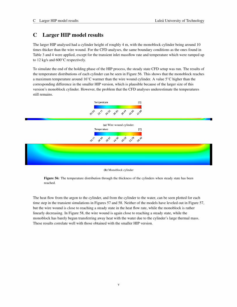
C Larger HIP model results Luleå University of Technology
C Larger HIP model results
The larger HIP analysed had a cylinder height of roughly 4 m, with the monoblock cylinder being around 10times thicker than the wire wound. For the CFD analyses, the same boundary conditions as the ones found inTable 3 and 4 were applied, except for the transient inlet massflow rate and temperature which were ramped upto 12 kg/s and 600◦C respectively.
To simulate the end of the holding phase of the HIP process, the steady state CFD setup was run. The results ofthe temperature distributions of each cylinder can be seen in Figure 56. This shows that the monoblock reachesa maximum temperature around 16◦C warmer than the wire wound cylinder. A value 5◦C higher than thecorresponding difference in the smaller HIP version, which is plausible because of the larger size of thisversion’s monoblock cylinder. However, the problem that the CFD analyses underestimate the temperaturesstill remains.
(a) Wire wound cylinder.
(b) Monoblock cylinder
Figure 56: The temperature distribution through the thickness of the cylinders when steady state has beenreached.
The heat flow from the argon to the cylinder, and from the cylinder to the water, can be seen plotted for eachtime step in the transient simulations in Figures 57 and 58. Neither of the models have leveled out in Figure 57,but the wire wound is close to reaching a steady state in the heat flow rate, while the monoblock is ratherlinearly decreasing. In Figure 58, the wire wound is again close to reaching a steady state, while themonoblock has barely begun transferring away heat with the water due to the cylinder’s large thermal mass.These results correlate well with those obtained with the smaller HIP version.
v

C Larger HIP model results Luleå University of Technology
Figure 57: A comparison of the heat flow from the argon gas to the cylinder at each time step for both thewire wound and monoblock model.
Figure 58: A comparison of the heat flow from the cylinder to the water at each time step for both the wirewound and monoblock model. The plot is showing negative values since the calculations are based on thecylinder surface which is giving off heat to the water.
In Table 9 is a summary of some results of interest from the transient CFD run. The monoblock column refersto the first case with water cooling on the outside of the cylinder. The differences between the cylinderversions can be compared with those obtained in the smaller HIP model, seen in Table 7. Because of the larger
vi

C Larger HIP model results Luleå University of Technology
size of this version’s cylinders, the numbers will differ somewhat, but the overall trend can be seen to besimilar between the two size’s results.
Table 9: A comparison of some numerical results between the two cylinder versions analysed of the largerHIP model.
Wire Wound Monoblock Difference [%]Argon outlet temperature [◦C] 345 366 6.1∆TArgon [◦C] 255 234 9.0∆TWater [◦C] 18 0.44 4000Total heat loss Argon→ Cylinder [kW] 1850 1740 6.3Total heat loss Cylinder→Water [kW] -958 -3.64 26 000Maximum temperature cylinder wall [◦C] 325 352 8.3
Regarding the FEM models of this larger HIP, the same boundary conditions as described in 3.3 are applicable,except for the wire pressure being 1800 bar. The von-Mises stress in each cylinder at the end time (300s) of thetransient CFD analyses is presented in Figure 59 and 60. These figures show that the wire wound cylinderexperiences the highest von-Mises stress around the bending caused by the mechanical pressures applied, thesame critical point as resulted in the smaller HIP version. This stress maximum is although disregarded, as it isbelieved to be caused by the sharp edges of the pressure areas, which is not an accurate representation ofreality. Except for this point, the critical area can be seen to agree with the temperature hot spot area, with thestress being around 908 MPa. In the monoblock model seen in Figure 60, the maximum stress also agrees withthe hot spot area, but with the stress being lower with a value of 632 MPa. The trend of these results agreeswell with the ones obtained in the smaller HIP version.
Figure 59: The von-Mises stress in the wire wound cylinder at the end time (300s).
vii

C Larger HIP model results Luleå University of Technology
Figure 60: The von-Mises stress in the monoblock cylinder at the end time (300s).
viii