Forschungsinstitut zur Zukunft der ArbeitInstitute for the Study of Labor

DI

SC

US

SI

ON

P

AP

ER

S

ER

IE

S

A Comparison of Panel Data Models inEstimating Technical Efficiency

IZA DP No. 9807

March 2016

Masoomeh RashidghalamAlmas HeshmatiGhader DashtiEsmail Pishbahar

A Comparison of Panel Data Models in Estimating Technical Efficiency

Masoomeh Rashidghalam University of Tabriz

Almas Heshmati

Sogang University and IZA

Ghader Dashti

University of Tabriz

Esmail Pishbahar

University of Tabriz

Discussion Paper No. 9807 March 2016

IZA

P.O. Box 7240 53072 Bonn

Germany

Phone: +49-228-3894-0 Fax: +49-228-3894-180

E-mail: iza@iza.org

Any opinions expressed here are those of the author(s) and not those of IZA. Research published in this series may include views on policy, but the institute itself takes no institutional policy positions. The IZA research network is committed to the IZA Guiding Principles of Research Integrity. The Institute for the Study of Labor (IZA) in Bonn is a local and virtual international research center and a place of communication between science, politics and business. IZA is an independent nonprofit organization supported by Deutsche Post Foundation. The center is associated with the University of Bonn and offers a stimulating research environment through its international network, workshops and conferences, data service, project support, research visits and doctoral program. IZA engages in (i) original and internationally competitive research in all fields of labor economics, (ii) development of policy concepts, and (iii) dissemination of research results and concepts to the interested public. IZA Discussion Papers often represent preliminary work and are circulated to encourage discussion. Citation of such a paper should account for its provisional character. A revised version may be available directly from the author.

IZA Discussion Paper No. 9807 March 2016

ABSTRACT

A Comparison of Panel Data Models in Estimating Technical Efficiency

The purpose of this paper is two-fold. First, it compares the performance of various panel data models in estimating technical efficiency in production. Second, it applies various stochastic frontier panel data models to estimate the technical efficiency of Iran’s cotton production and to provide empirical evidence on the sources of technical inefficiency of cotton producing provinces. The results indicate that labor and seeds are determinants of cotton production and inorganic fertilizers result in reducing technical efficiency. The mean technical efficiency of the models is around 80 percent. Variations in the distribution of estimated efficiency amongst the different models is large. JEL Classification: C23, D24, Q12 Keywords: technical efficiency, labor use, panel data modeling, time-variant,

persistent inefficiency, individual heterogeneity, model comparison, cotton production, Iran

Corresponding author: Almas Heshmati Department of Economics Sogang University Baekbeom-ro (Sinsu-dong #1), Mapo-gu Seoul 121-742 Republic of Korea E-mail: heshmati@sogang.ac.kr

2  

1. Introduction

Stochastic frontier models are consistent with the objective of output maximization or input minimization in production. In recent decades there has been increased availability of panel data which has led to a surge in stochastic frontier panel data methodologies aimed at estimating technical efficiency in production. These models differ in the way in which they account for various aspects of production to generate consistent and unbiased estimates. Literature has developed enough to account for time-variance, heteroscedastic, persistent technical efficiency effects, separation of inefficiency and individual effects and identification of determinants of inefficiency and estimations of their effects. A few studies also compare the performance of panel data models using the same panel dataset (Kumbhakar and Heshmati, 1995; Greene, 2015a, 2005b; Emvalomatis, 2009; Wang and Ho, 2010; Kumbhakar et al., 2014). This study contributes to the existing literature by comparing all existing stochastic frontier panel data models using same panel dataset.

Iran is the second largest economy in the Middle East and North African region after Saudi Arabia, with an estimated gross domestic product of $406.3 billion in 2014. Unlike Saudi Arabia, Iran’s economy is diversified with agriculture and industry sectors having large shares. It also has the second largest population (78.5 million people in 2014) in the region after Egypt. Iran’s economy is composed of a large hydrocarbon sector, small scale agriculture and services sectors and a noticeable state presence in manufacturing and financial services. It ranks second and fourth in natural gas and proven crude oil reserves in the world respectively.1

Influenced by recent decades of frequent economic and technological sanctions against the country and the Iran-Iraq war in the 1980s, food security is a top national priority in the country. This implies pursuing: (i) reliance on national resources through higher domestic productivity and self-sufficiency in staple crops and animal products, and (ii) improving food consumption patterns through an increasing share of animal protein intake. Food availability shows signs of improvement due to increased productive capacity in the main food crops along a ten-year reform period (2000-2010). However, the production is not sufficient to meet domestic demand which is met only through complementary imports. Linked to the goal of food security is enhancing the productivity of Iran’s agriculture. This objective may be interpreted both in terms of increasing total agricultural production and in terms of increasing productivity of factors so that productivity gains may account for at least 2.6 per cent of the country’s economic growth. Productivity gains should be expressed both in terms of enhancing per hectare productivity due to higher efficiency of agricultural land and enhancing water use productivity in the agriculture sector (FAO, 2012).

Cotton is one of the most important fiber producing plants in the world. This crop not only provides fiber for the textile industry, but also plays an important role in the feed and oil industries with its

                                                            1 For an overview of the Iran’s economy see http://www.worldbank.org/en/country/iran/overview

3  

seeds, which are rich in oil (18-24 per cent) and protein (20-40 per cent). An estimated 350 million people around the world are engaged in cotton production either on-farm or in transportation, ginning, baling and storage. Annually 25 million tons of cotton is produced in the world, around 80 per cent of which is in China, the United States of America, Pakistan, India and Uzbekistan (FAO, 2010).

The total area under cotton production in Iran in 2012 was about 123,000 hectares. Most cultivated areas devoted to cotton production are located in the Khorasan (31 per cent) and Golestan (15.3 per cent) provinces. Total cotton production was about 337,000 tons, of which 86,837 tons were produced in Khorasan and 61,742 tons were produced in Fars provinces. The production per hectare in Fars province is higher than in Golestan. Since industries in Iran need double the amount of present production levels, most of which is provided through imports. Considering the urgent need for increasing cotton production and due to limited supply of arable land, this study uses the stochastic production function methodology to study the technical efficiency of Iran’s cotton production using panel data for provinces. This study also provides empirical evidence on the sources of technical inefficiencies and gives policy recommendations for increasing cotton production.

The frontier function methodology has been given particular attention for measuring and comparing the performance of individual production units within a geographic location, an industry or a service sector. Extensive research in this field has resulted in the rapid development of econometric techniques concerning specifications, estimations and testing issues. These techniques have been rapidly developed and implemented in a large number of areas using mostly cross-sectional micro data. Methods have also been developed to estimate firm efficiency using panel data. Some of the problems related to distributional assumptions encountered in the cross-section approach are avoided in panel data models. Panels also give a large number of data points and have the advantage of separating individual and time-specific effects from the combined effect (Heshmati et al., 1995).

Another advantage of panel data is that if inefficiency is time-invariant one can estimate inefficiency consistently without distributional assumptions (Schmidt and Sickles, 1984). The assumption that inefficiency is time-invariant is quite strong, although the model is relatively simple to estimate if efficiency is specified as a fixed parameter instead of as a random variable (Battese and Coelli, 1988; Kumbhakar, 1987; Pitt and Lee, 1981). The other extreme is assuming that both inefficiency and noise terms are independently and identically distributed (i.i.d.). This assumption makes the panel nature of the data irrelevant. There are also models that fall between these extreme (Kumbhakar et al., 2014).

This paper does two main things: First, it compares the performance of various panel data models for estimating technical efficiency in production. Second, it applies various stochastic frontier panel data models to estimate the technical efficiency of cotton production in Iran and provides

4  

evidence on the sources of technical inefficiencies in its production. The empirical analysis uses panel data from Iran’s cotton producing provinces for 2000-12. The results indicate that labor and seeds are the main determinants of cotton production and that inorganic fertilizers result in reducing technical efficiency. The mean technical efficiency in most models was found to be around 80 per cent, but variations in distribution and across provinces were large. These can be attributed to the impact that geography and management have on technical efficiency. The result provides researchers a picture of the performance of different models; it also provides policymakers an estimate of efficiency in cotton production in each province.

The remainder of this paper is organized into five sections. First, we present the methodological framework adopted in this study which is followed by a description of the data and empirical model specifications. Next we present the results and policy recommendations. The last section gives the conclusions.

2. Methodology

The stochastic frontier approach for estimating technical efficiency is based on the idea that an economic unit may operate below its production frontier due to errors and some uncontrollable factors. A study of the frontier started with Farrell (1957) who suggested that efficiency could be measured by comparing realized output with the maximum attainable output. Later, based on Farrell’s efficiency notion Aigner et al. (1977) and Meeusen and van den Broeck (1977) independently proposed stochastic frontier models (Emvalomatis, 2009).

Estimating inefficiency in these models requires distributional assumption unless one uses the corrected ordinary least squares (COLS) and makes the assumption that there is no noise. Schmidt and Sickles (1984) discuss three problems with cross-sectional models that are used to measure inefficiency. First, the maximum likelihood (ML) estimation method which is used for estimating parameters and inefficiency estimates using the Jondrow, Lovell, Materov and Schmidt (1982) formula depends on the distributional assumption of noise and inefficiency components. Second, the technical inefficiency component has to be independent of the regressors (at least in the single equation models) – an assumption that is unlikely to be true if a firm maximizes profits and also knows its level of inefficiency. Third, the Jondrow et al. (1982) estimator is not consistent.

If panel data are available, that is, each unit is observed at several different points of time some of these limitations can be removed. However, to overcome some of these limitations, the panel models require other assumptions, some of which may or may not be realistic (Kumbhakar et al., 2015). Thus, both costs and benefits are associated with the use of panel data for measuring performance.

A key advantage of panel data is that it enables the modeler to take into account some heterogeneity that may exist beyond what is possible to control using a cross-sectional approach which lumps

5  

individual effects with random errors. This can be achieved by introducing an ‘individual

(unobservable) effect’, say, , that is time-invariant and individual-specific, and which has not interacted with other variables.

Having information on units over time also enables one to examine whether inefficiency has been persistent over time or whether the inefficiency of units is time-varying. There may be a component of inefficiency that has been persistent over time and another that is varied over time. Related to this, and a key question that needs to be considered with regard to time-invariant individual effects, is whether an individual effect represents (persistent) inefficiency, or whether the effects are independent of inefficiency and capture (persistent) unobserved heterogeneity. A second question related to this is whether individual effects are fixed parameters or are realizations of a random variable (Kumbhakar et al., 2015). Thus, information about persistence and time-variance of inefficiency effects and their separation from unobserved heterogeneity effects is important in policymaking for promoting efficiency in the production of scarce resources.

In this study we outline 12 panel data models grouped into four groups in terms of the assumptions made on the temporal behavior of inefficiency. A common issue among all the models is that inefficiency is individual-specific. This is consistent with the notion of measuring efficiency of decision-making units. Models 1 to 3 assume the inefficiency effects to be time-invariant and individual-specific. Models 4 to 7 allow inefficiency to be individual-specific but time-varying. Models 8 to 10 separate inefficiency effects from unobserved individual effects. Finally, models 11 and 12 separate persistent inefficiency and time-varying inefficiency from unobservable individual effects. In general, all performance measurement methods are expected to generate individual-specific effects. Thus, in continuation we focus on the time-variance of inefficiency effects and their separation from non-inefficiency heterogeneity effects.

2.1 Models with time-invariant inefficiency effects

Model 1:

We first consider the case in which inefficiency is assumed to be individual-specific but time-invariant. In this case the model can be estimated assuming that either the inefficiency component

(u ) is a fixed parameter (the fixed-effects model) or a random variable (the random-effects model). The fixed-effects model can be written as (Schmidt and Sickles, 1984):

(1) ititi

iititit

xu

uxy

)( 0

0

(2) ititi x                 

where is the log of output for province i at time t; β is a common intercept; x is the vector of

inputs (in logs); β is the associated vector of technology parameters to be estimated; v is a random

6  

two-sided noise term that can increase or decrease output (ceteris paribus); and u 0 is the non-negative one-sided inefficiency term. The model in (2) looks similar to a standard fixed-effects

(FE) panel data model.

Once are available, the following transformation is used to obtain an estimated value of

(Schmidt and Sickles, 1984):

(3) ,0ˆˆmaxˆ iiiiu Ni ,...,1

This formulation implicitly assumes that the most efficient unit in the sample is 100 per cent efficient. If one is interested in estimating firm-specific efficiency, it can be obtained from the relation:

(4) ),ˆexp(ˆiuET Ni ,...,1

The weakness of this model is its strong assumption of time-invariant inefficiency and inability to separate inefficiency and individual heterogeneity.

Model 2:

Instead of assuming α (and thus u ) in (2) as fixed parameters, it is also possible to assume that α

is random and uncorrelated with the regressors. If the assumption of no correlation is indeed correct, then the random-effect (RE) model provides more efficient estimates than the FE model. The RE model can be estimated by two different methods: One, by estimating it by the generalized least squares (GLS) technique commonly used for a standard RE panel data model. Like the FE estimator, RE is modified and re-interpreted to obtain estimates of inefficiency.

Now assume u is a random variable and let E u μ and u ∗ u μ . We rewrite the model as:

(5) *

0

0

)( iitit

iititit

ux

uxy

,**iitit ux                           

where ∗ β μ. The advantage of this model compared with Model 1 is that it allows for testing the assumption of fixed or random inefficiency and provides a possibility for estimating the model efficiently.

Model 3:

7  

An alternative to the GLS method is imposing distributional assumptions on the random components of the model, and estimating the parameters by the maximum likelihood (ML) method (Pitt and Lee, 1981).

For ML, the model is written as:

(6)

).,0(~

),,0(~

,

,),(

2

2

ui

vit

iitit

ititit

Nu

N

uv

xfy

Through the iteration procedure, the ML estimation method generates higher efficiency in estimation but at the cost of strong assumptions of normality of the random error term.

2.2 Models with time-variant inefficiency effects

Model 4:

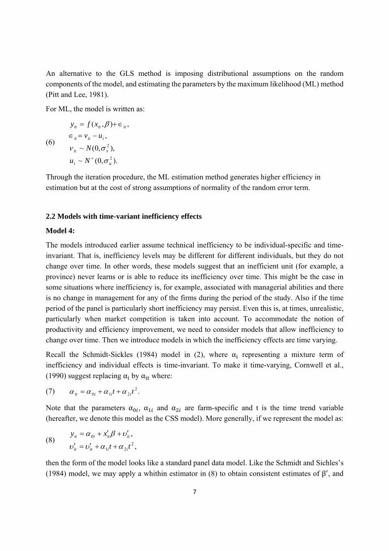
The models introduced earlier assume technical inefficiency to be individual-specific and time-invariant. That is, inefficiency levels may be different for different individuals, but they do not change over time. In other words, these models suggest that an inefficient unit (for example, a province) never learns or is able to reduce its inefficiency over time. This might be the case in some situations where inefficiency is, for example, associated with managerial abilities and there is no change in management for any of the firms during the period of the study. Also if the time period of the panel is particularly short inefficiency may persist. Even this is, at times, unrealistic, particularly when market competition is taken into account. To accommodate the notion of productivity and efficiency improvement, we need to consider models that allow inefficiency to change over time. Then we introduce models in which the inefficiency effects are time varying.

Recall the Schmidt-Sickles (1984) model in (2), where α representing a mixture term of inefficiency and individual effects is time-invariant. To make it time-varying, Cornwell et al.,

(1990) suggest replacing α by α where:

(7) .2210 tt iiiit

Note that the parameters α , α and α are farm-specific and t is the time trend variable (hereafter, we denote this model as the CSS model). More generally, if we represent the model as:

(8) ,

,2

21

0

tt

xy

iiitit

ititiit

then the form of the model looks like a standard panel data model. Like the Schmidt and Sichles’s

(1984) model, we may apply a whithin estimator in (8) to obtain consistent estimates of β , and

8  

then the estimated residuals of the model ( ̂ x β ). A disadvantage of this model is that

the time-variant is a function of a time trend and as such it is unable to capture possible (non-trend) fluctuations in inefficiency over longer periods.

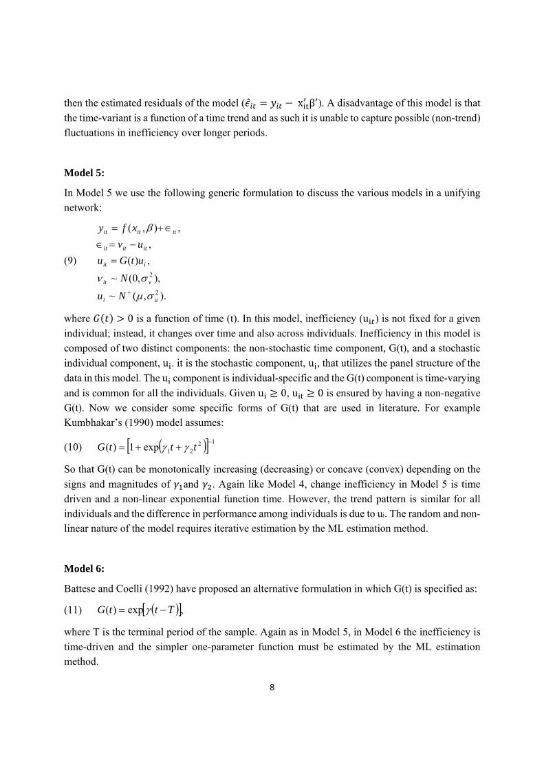
Model 5:

In Model 5 we use the following generic formulation to discuss the various models in a unifying network:

(9)

).,(~

),,0(~

,)(

,

,),(

2

2

ui

vit

iit

ititit

ititit

Nu

N

utGu

uv

xfy

where 0 is a function of time (t). In this model, inefficiency (u ) is not fixed for a given individual; instead, it changes over time and also across individuals. Inefficiency in this model is composed of two distinct components: the non-stochastic time component, G(t), and a stochastic

individual component, u . it is the stochastic component, u , that utilizes the panel structure of the

data in this model. The u component is individual-specific and the G(t) component is time-varying

and is common for all the individuals. Given u 0, u 0 is ensured by having a non-negative

G(t). Now we consider some specific forms of G(t) that are used in literature. For example Kumbhakar’s (1990) model assumes:

(10) 1221exp1)(

tttG

So that G(t) can be monotonically increasing (decreasing) or concave (convex) depending on the

signs and magnitudes of and . Again like Model 4, change inefficiency in Model 5 is time driven and a non-linear exponential function time. However, the trend pattern is similar for all individuals and the difference in performance among individuals is due to ui. The random and non-

linear nature of the model requires iterative estimation by the ML estimation method.

Model 6:

Battese and Coelli (1992) have proposed an alternative formulation in which G(t) is specified as:

(11) ,exp)( TttG

where T is the terminal period of the sample. Again as in Model 5, in Model 6 the inefficiency is

time-driven and the simpler one-parameter function must be estimated by the ML estimation method.

9  

Model 7:

Kumbhakar and Wang (2005) use the following specification to specify a model of time-variant

efficiency driven by time:

(12) ,exp)( tttG

where is the beginning period of the sample. This is the opposite of Model 6 where T represents

the last period of observation. The reference points in these two models are the initial and final

periods. Analytically (11) and (12) are the same, but they are interpreted differently. In Battese

and Coelli (1992) and the reformulated specification by Kumbhakar (1990), u ~N μ, σ

specifies the distribution of inefficiency at the terminal point, that is,u u when . With

(12), u ~N μ, σ specifies the initial distribution of inefficiency. The strength of Model 6 is in

accounting for market entry, while accounts for market exit in formulating the reference point in

Model 7. A mixture model formulation of the two initial and terminal reference points might be

superior to the two models individually.

2.3 Models separating inefficiency and unobserved individual effects

Models 8 and 9:

The model as specified in (1) and (2) is a standard panel data model where α is an unobservable

individual effect. Standard panel data fixed and random-effects estimators are applied to estimate

the model parameters including α . The only difference is that we transform the estimated value

of α to obtain the estimated value of u , namely u by using the highest α as a reference for the

frontier.

A notable drawback of this approach is that individual heterogeneity cannot be distinguished from inefficiency. In other words, all time-invariant heterogeneity such as soil quality that is not

necessarily inefficient is included as inefficiency, and therefore u might be picking up

heterogeneity in addition to or even instead of inefficiency (Greene, 2005b; Kumbhakar and

Heshmati, 1995). Outliers serving as a reference and confounded inefficiency can overestimate or bias performance estimates.

Another potential issue with the models (1) and (2) is the time-invariant assumption of inefficiency. If T is large, it seems implausible that the inefficiency of a firm may stay constant for

an extended period of time and that a firm with persistent inefficiency will survive in the market. So should one view the time-invariant component as persistent inefficiency or as individual

heterogeneity that captures the effects of time-invariant covariates and has nothing to do with inefficiency? If the latter is true, then the results from the time-invariant inefficiency models are wrong. Perhaps the truth lies somewhere in between. That is, a part of the inefficiency might be

10  

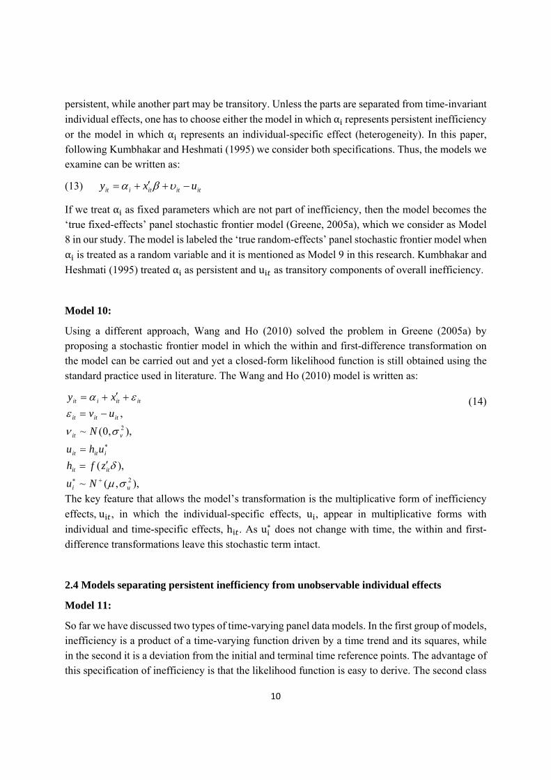
persistent, while another part may be transitory. Unless the parts are separated from time-invariant

individual effects, one has to choose either the model in which α represents persistent inefficiency

or the model in which α represents an individual-specific effect (heterogeneity). In this paper,

following Kumbhakar and Heshmati (1995) we consider both specifications. Thus, the models we examine can be written as:

(13) itititiit uxy

If we treat α as fixed parameters which are not part of inefficiency, then the model becomes the

‘true fixed-effects’ panel stochastic frontier model (Greene, 2005a), which we consider as Model 8 in our study. The model is labeled the ‘true random-effects’ panel stochastic frontier model when

α is treated as a random variable and it is mentioned as Model 9 in this research. Kumbhakar and

Heshmati (1995) treated α as persistent and u as transitory components of overall inefficiency.

Model 10:

Using a different approach, Wang and Ho (2010) solved the problem in Greene (2005a) by proposing a stochastic frontier model in which the within and first-difference transformation on the model can be carried out and yet a closed-form likelihood function is still obtained using the

standard practice used in literature. The Wang and Ho (2010) model is written as:

(14)

The key feature that allows the model’s transformation is the multiplicative form of inefficiency

effects,u , in which the individual-specific effects, u , appear in multiplicative forms with

individual and time-specific effects, h . As u∗ does not change with time, the within and first-

difference transformations leave this stochastic term intact.

2.4 Models separating persistent inefficiency from unobservable individual effects

Model 11:

So far we have discussed two types of time-varying panel data models. In the first group of models, inefficiency is a product of a time-varying function driven by a time trend and its squares, while

in the second it is a deviation from the initial and terminal time reference points. The advantage of this specification of inefficiency is that the likelihood function is easy to derive. The second class

),,(~

),(

),,0(~

,

2

2

ui

itit

iitit

vit

ititit

ititiit

Nu

zfh

uhu

N

uv

xy

11  

of models examined controlled for firm-effects and allowed inefficiency to be time-varying. Unfortunately, these two classes of models are not nested and, therefore, the data cannot help one in testing to choose which formulation is appropriate.

However, both these classes of models view firm effects (fixed or random) as something different from inefficiency. That is, inefficiency in these models is always time-varying and can either be i.i.d. or a function of exogenous variables. Thus, these models fail to capture persistent inefficiency, which is hidden within firm effects. Consequently, these models are mis-specified and tend to produce a downward bias in the estimate of overall inefficiency, especially if persistent inefficiency exists and its magnitude is significant. Models 11 and 12 separate persistent and time-varying inefficiency components. Identifying the magnitude of persistent inefficiency is important, especially in short panels, because it reflects the effects of inputs like management (Mundlak, 1961) and other unobserved inputs which vary across firms but not over time. The residual component of inefficiency might change over time without any change in a firm’s operations. Therefore, a distinction between the persistent and residual components of inefficiency is important and thus they have different policy implications. Thus, our Model 11 is the Kumbhakar and Heshmati (1995) model that is specified as:

(15)

itiit

ititit

ititit

uu

u

xy

0

The technical inefficiency part is decomposed as u u τ where u is the persistent

component (for example, time-invariant management effects) and τ is the residual (time-varying) component of technical inefficiency, both of which are non-negative. The former is only firm-specific, while the latter is both firm and time-specific. To estimate the model we rewrite (15) as:

(16)

))((

)(0

itititit

itii

ititiit

E

andEuA

xy

The error components,ω , have zero mean and constant variance. The model can be estimated either by the least squares dummy variable approach or by the generalized least squares (GLS) method. Following Kumbhakar and Heshmati (1995) we use a multi-step procedure to estimate the model. In step 1, we estimate (16) using the standard fixed-effects panel data model to obtain

consistent estimates of β. In step 2, we estimate persistent technical inefficiency, u . In step 3, we

estimate β and the parameters associated with the random components, v and τ . Finally, in

step 4, the time-varying (residual) component of inefficiency,τ , is estimated. The multi-step procedure is cumbersome, but has the advantage of avoiding strong distributional assumption by estimating the model using the ML estimation method.

12  

Model 12:

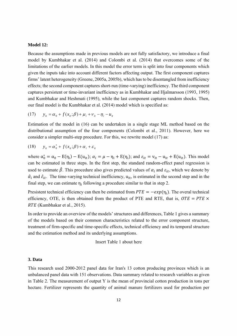
Because the assumptions made in previous models are not fully satisfactory, we introduce a final model by Kumbhakar et al. (2014) and Colombi et al. (2014) that overcomes some of the limitations of the earlier models. In this model the error term is split into four components which given the inputs take into account different factors affecting output. The first component captures firms’ latent heterogeneity (Greene, 2005a, 2005b), which has to be disentangled from inefficiency effects; the second component captures short-run (time-varying) inefficiency. The third component captures persistent or time-invariant inefficiency as in Kumbhakar and Hjalmarsson (1993, 1995) and Kumbhakar and Heshmati (1995), while the last component captures random shocks. Then, our final model is the Kumbhakar et al. (2014) model which is specified as:

(17) itiitiitit uxfy );(0

Estimation of the model in (16) can be undertaken in a single stage ML method based on the distributional assumption of the four components (Colombi et al., 2011). However, here we consider a simpler multi-step procedure. For this, we rewrite model (17) as:

(18) itiitit xfy );(0

where α∗ α E η E u ; η E η ; and v u E u . This model can be estimated in three steps. In the first step, the standard random-effect panel regression is

used to estimate . This procedure also gives predicted values of and , which we denote by

and ̂ . The time-varying technical inefficiency, u , is estimated in the second step and in the

final step, we can estimate η following a procedure similar to that in step 2.

Presistent technical efficiency can then be estimated from η . The overal technical

efficiency, OTE, is then obtained from the product of PTE and RTE, that is,

(Kumbhakar et al., 2015).

In order to provide an overview of the models’ structures and differences, Table 1 gives a summary of the models based on their common characteristics related to the error component structure, treatment of firm-specific and time-specific effects, technical efficiency and its temporal structure and the estimation method and its underlying assumptions.

Insert Table 1 about here

3. Data

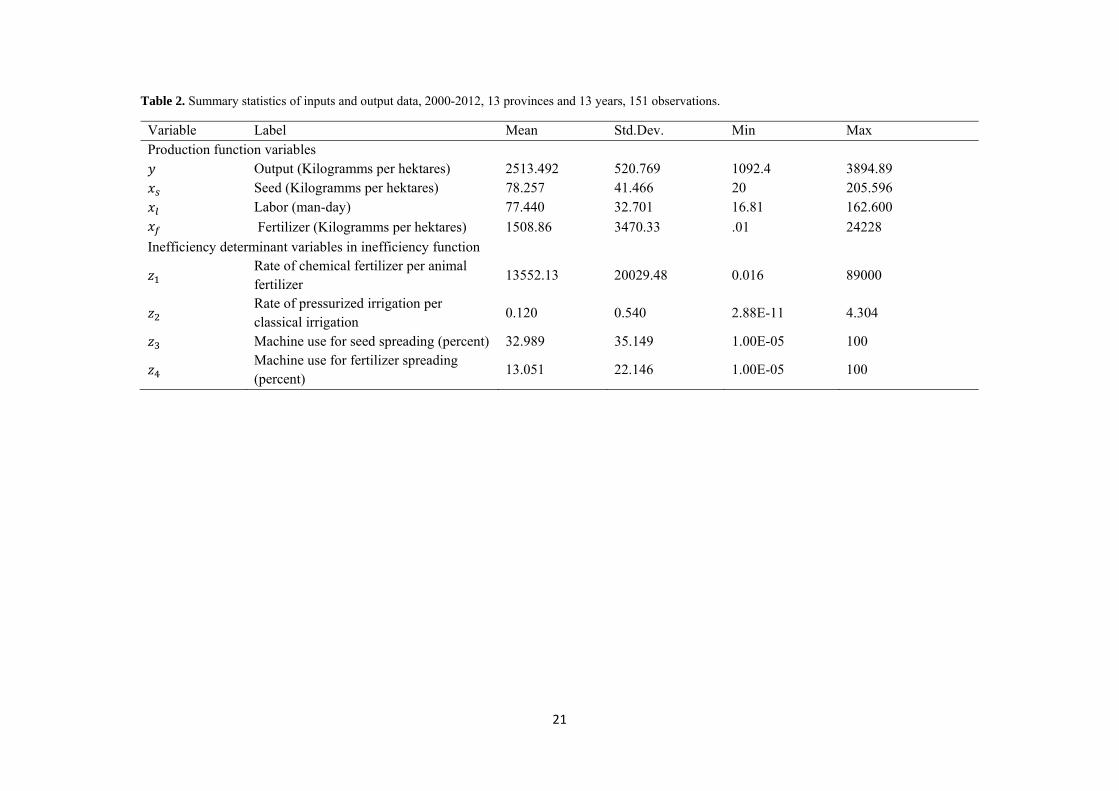
This research used 2000-2012 panel data for Iran's 13 cotton producing provinces which is an unbalanced panel data with 151 observations. Data summary related to research variables as given in Table 2. The measurement of output Y is the mean of provincial cotton production in tons per hectare. Fertilizer represents the quantity of animal manure fertilizers used for production per

13  

hectare. Measurement for labor input L is the total number of employees per hectare in different provinces. Seed represent kilograms of seeds and seedlings per hectare. The data used for this paper came from Iran’s Ministry of Agriculture Jihad, where the data are collected regionally through an annual survey that uses a common questionnaire across all provinces. The summary statistics of the data is provided in Table 1. The table shows that cotton production varied between a minimum of 1,092 kg to a maximum of 3,895 kg per hectare in the different provinces, and mean cotton production was about 2,513 kg per hectare. Seed consumption ranged between 20 to 205 kg per hectare with a standard deviation of 41.47 among provinces. The number of labor per hectare was about 77, which may reflect the fact that cotton production is labor intensive in Iran. Organic fertilizer usage decreased over time. This reflects the trend that young farmers are more likely to use chemical fertilizers and overlook the importance of organic manure.

Insert Table 2 about here

4. Analysis of the Results

4.1 Specification and estimation testing and model selection

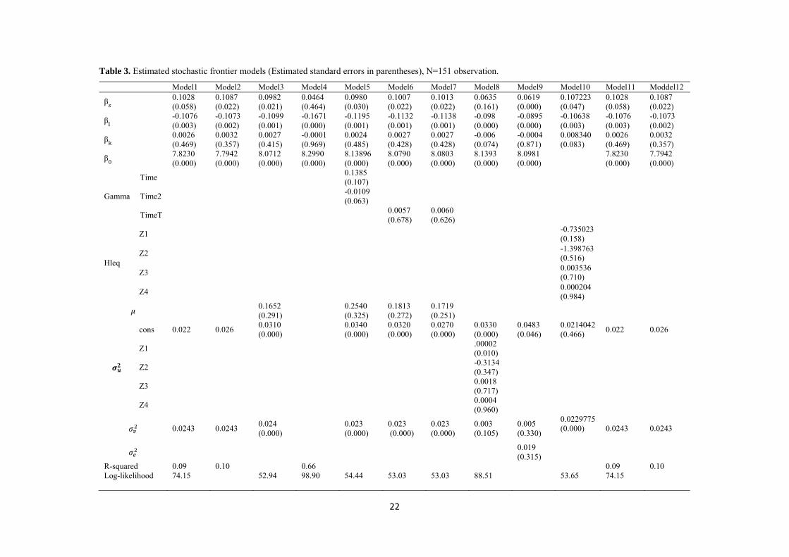
For the purposes of this study, we analyzed a Cobb–Douglas production function for Models 1-12. A simple functional form was chosen for a number of reasons. First, the main objective was to investigate the sensitivity of efficiency results across different specifications and decomposition of technical efficiency. This can be achieved more easily with a simple functional form. Second, the implications of assumptions regarding efficiency and its decomposition were easier to investigate within the frame of a simple functional form. Third, we were interested in average elasticities which are obtained without employing a flexible function form. The estimation results are given in Table 3.

Insert Table 3 about here

For comparing some nested models we used a generalized likelihood ratio (LR) test. Based on the results of this test in Table 4, Model 5 was rejected in favor of the time-invariant model (Model 3). Given the results of the statistical tests this table suggests that the time-invariant model was preferred to the time decay model (Model 6) and Model 7. The results discussed earlier imply that technical efficiency measures do not appear to be affected by time.

Insert Table 4 about here

4.2 Analysis of results from selected models

For all models the estimated output elasticity with respect to labor was negative and statistically significant, indicating that production decreased with such inputs. The negative sign implies that by increasing inputs by k-times, provinces will get less output than current levels. In other words

14  

provinces will pay more to get less. This may be due to labor application in the third stage of production when it should already be decreased. Increase in seed use will lead to an increase in cotton output which is statistically significant in all models except Models 4, 5 and 8. This indicates the importance of seeds in cotton production. The elasticity of output with respect to fertilizers is negative but insignificant.

The negative elasticities for labor and fertilizers reported in this paper are consistent with other studies. Mohammed and Saghaian (2014) found negative elasticity for these two inputs in rice production in Korea and Chakraborty et al., (2002) concluded that fertilizers and machinery had negative effects on cotton production in irrigated farms in Texas. Wan and Cheng (2001) and Chen et al. (2003) found excessive labor usage in Chinese agriculture. Their study focused on an analysis of efficiency in production rather than output responsiveness to input utilization. In terms of policy implications it is more important to determine which variables lead to inefficiency. The variables considered in current study to identify possible influences on technical efficiency are chemical fertilizers versus animal fertilizers, pressurized irrigation versus classical irrigation and machine use for seed and fertilizer spreading to indicate the extent to which farms use modern production technologies.

The positive sign of the parameters of these variables in Table 4 means the associated variables have a negative effect on technical efficiency. According to this table use of more inorganic fertilizers than organic ones leads to a significant decrease in technical efficiency. Unpressurized irrigation versus classical irrigation was used in order to investigate whether technical efficiency increased when more machinery was used in irrigation of cotton farms. The result shows that it led to an insignificant increase in technical efficiency in cotton production. Probably the reason for this is that there is not much difference between provinces when it comes to using irrigation technology. The results also suggest that the current extension program should be reoriented to give more emphasis to the application of inputs and production practices.

Descriptive statistics for technical efficiency according to different models are presented in Table 5. According to this table, various models clearly produced different results. Mean technical efficiency of Model 10 was the highest, while it was the least for Model 9. The average technical efficiency for Models 1 and 2 was about 0.80 with a maximum of 1, while the minimum for Model 1 was 0.65 and for Model 2 it was 0.64. Therefore, the gap between the most efficient and inefficient provinces was about 0.35. This gap states the difference between provinces in input allocations for cotton production. The mean value of technical efficiency according to most of the models was more than 0.80. The average efficiency indices reported in this study are within the bounds of those found in other studies on efficiency of cotton farms. Using farm-level data from four counties in west Texas, Chakraborty et al., (2002) estimated average efficiency as 80 per cent. Another study of cotton production found average technical efficiency of 79 per cent for farms in Çukurova region in Turkey (Gul et al., 2009).

15  

Insert Table 5 about here

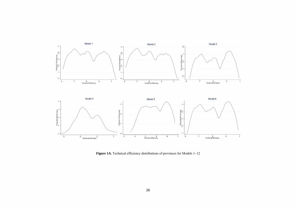
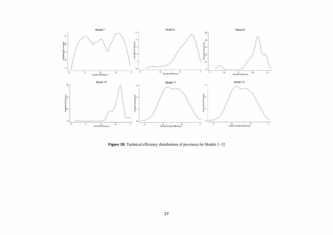
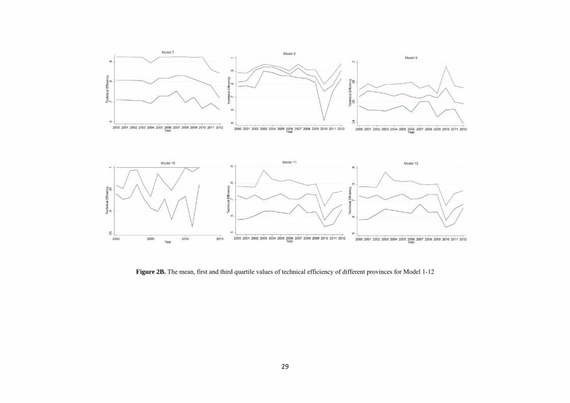
Figure 1 presents kernel density distribution of technical efficiency estimates for Models 1-12. As an example, consider Models 5 and 6, in which the distribution of technical efficiency scores range from 0.59 to 0.94 and 0.64 to 0.95 respectively. Figure 2 illustrates the lower quartile, median and upper quartile efficiencies over time across 12 models, in which the spread of the efficiency can be seen. According to this figure Model 4 had the widest efficiency and Model 8 had the narrowest spread, slightly narrower than Model 9. As Figure 2 shows, the time-series pattern for most of the models is similar. Due to unbalanced panel data, mean of efficiency in time-invariant models (Models 1-3) was not constant.

Insert Figure 1 about here

Insert Figure 2 about here

For an investigation of the performance of different sample provinces and their position compared with the province with the best practiced technology, we would rank the provinces. Descriptive statistics for technical efficiency measured by provinces are presented in Table 6. Estimated efficiency measures for different models reveal that there are differences between provinces in terms of efficiency. For example, estimated technical efficiency according to Model 1 in East Azerbaijan and Kerman provinces was 100 and 65 per cent respectively. On the other hand, technical efficiency was estimated to be the highest for East Azerbaijan, Esfahan, Ardebil and Tehran and the lowest for Kerman, Mazandaran, Golestan and Khorasan. So we conclude that there is the possibility of increasing cotton production in different provinces through better input and extension practices.

Insert Table 6 about here

The results show that different ranks for provinces determined by the 12 models. All the models except Models 8, 9 and 10 showed consistent rankings among provinces. The yearly mean of provincial technical efficiency for the 12 models is presented in Table 7. There were some variations in technical efficiency over time. According to most of the models, technical efficiency decreased during the period; 2007 was the most efficient year and 2012 the most inefficient year during the study period. The value of technical efficiency according to all models, except Model 10, for the entire period was quite high and was mostly concentrated in an interval of 60-92 per cent.

Insert Table 7 about here

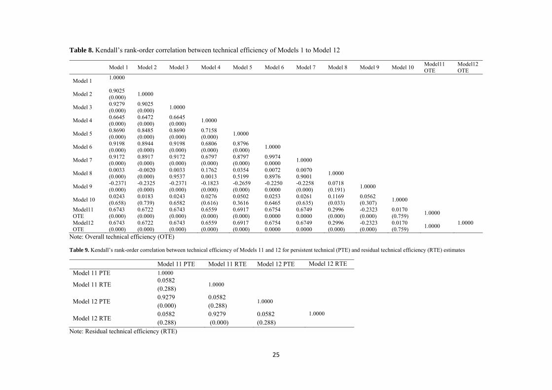
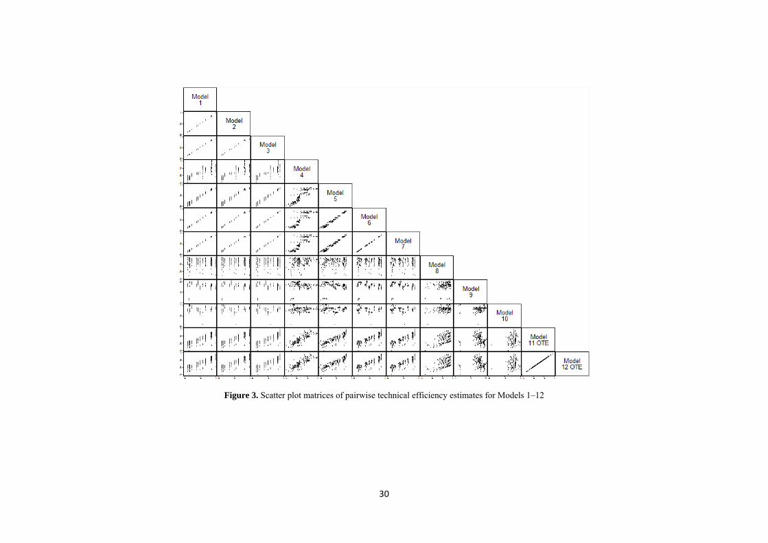
Pairwise rank order correlations of Models 1 to12 are reported in Table 8. There is a perfect match between Models 11 and 12. The correlation between Models 6 and 7, and also between Models 1, 2 and 3 was high. These models seem to be the most consistent in generating similar results, while the results of technical efficiency estimates between Model 10 and Models 1-9 and also between Model 8 and Models 1-7 are to a large extent independent, with a rank-order correlation of less

16  

than 0.05. In Figure 3 scatter plot matrices for Models 1-12 graphically illustrate the differences between the models in the ranking of the provinces. The straight lines in the graph indicate a perfect match between two compared models. These results prove the findings as given in Table 8.

Insert Table 8 about here

Insert Figure 3 about here

Table 9 shows Kendall’s rank-order correlation for the persistent technical efficiency measure between Models 11 and 12. According to this table, assessments of residual technical efficiency for these two models are to a large extent positively correlated, with a rank-order correlation of 0.92. The results based on persistent and residual technical efficiency are independent, with a rank-order correlation of 0.05.

Insert Table 9 about here

4.3 Policy recommendations

The results of our research are important as they provide detailed information to policymakers. Our recommendations for policymakers include:

There is a need to use efficient machinery to reduce the labor’s contribution in cotton production in Iran in order to enhance productivity.

Rate of use of inorganic fertilizers as compared to organic fertilizers was negatively related to efficiency, implying that implementing policies will reduce inorganic fertilizer usage. Such a decision will help remove the subsidy given to chemical fertilizers.

Emphasis should be placed on strengthening the capacity of cotton farmers through farmer training workshops geared towards managerial and resource use efficiency. This should be done in a collaborative manner involving the government, district assemblies and NGOs.

Large differences between regions show provincial disparities, which in turn indicate that location has a significant impact on the efficiency of cotton production in Iran. One reason for this could be the environmental conditions that exist in different parts of the country. This implies further research which considers geographical conditions in measuring technical efficiency in different zones.

5. Conclusion

This paper investigated the technical efficiency of cotton production and its determinants in Iran’s main cotton producing provinces. Twelve stochastic production frontier models were estimated. The models differed in their underlying assumptions of time-variant/invariant technical efficiency and its decomposition as well as separation of technical inefficiency and province heterogeneity effects. The models incorporated almost all previously used model specifications. Estimating the

17  

models by using the same data allows shedding light on each model’s strengths and weaknesses. This analysis was applied to 13 cotton producing provinces which were observed over a period of 13 years (2000-2012).

This study came to the conclusion that labor and seeds are significant determinants of output in cotton production, and only seeds positively influence production. The negative significance of labor indicates labor-hoarding behavior which makes the provinces use more labor during the production season for which they get less returns.

Empirical results of an investigation of the sources of technical inefficiency showed that the rate of use of chemical fertilizers equivalent to per unit use of animal fertilizers was a determining factor in technical inefficiency in production. Inorganic fertilizers result in reducing technical efficiency. Therefore, it is possible to increase technical efficiency if more organic fertilizers rather than inorganic fertilizers are used.

The results also emphasize that according to most of the models mean technical efficiency was about than 80 per cent of the best practiced technology. Average technical efficiency measures suggest that cotton producing provinces in Iran could increase their production by about 20 per cent through more efficient use of inputs, in particular by using organic fertilizers.

This paper also discussed the different levels of technical efficiency among various provinces in the country. The empirical results show evidence of large differences in technical efficiency levels between provinces, which shows that the impact of geography and management on technical efficiency is quite heterogeneous in different provinces. According to most of the models, East Azerbaijan, Esfahan and Ardebil were the most efficient provinces for cotton production. Results also indicate that technical efficiency decreased during the study period.

REFRENCES

Aigner, D., Lovell, C.A.K., and P. Schmidt (1977). Formulation and estimation of stochastic frontier production functions. Journal of Econometrics, 6(1), 21–37.

Battese, G.E. and T.J. Coelli (1988). Prediction of firm-level technical efficiencies with a generalized frontier production function and panel data. Journal of Econometrics, 38, 387–399.

Chakraborty, K., S. Mirsa and P. Johnson. (2002). Cotton farmers’ technical efficiency: stochastic and nonstochastic production function approaches. Agricultural and Resource Economics Review, 31(2), 211-220.

Chen, A. Z., W. E., Huffman and S. Rozelle (2003). Technical Efficiency of Chinese Grain Production: A Stochastic Production Frontier Approach, Paper prepared for presentation at

18  

the American Agricultural Economics Association Annual Meeting, Montreal, Canada, July 27-30.

Colombi. R., Martini, G. and G. Vittadini (2011). A stochastic frontier model with short-run and long-run inefficiency random effects. Department of Economics and Technology Management, Universita di Bergamo, Italy.

Colombi, R., Khumbakhar, S.C., Martini, G. and G. Vittadini (2014). Closed-Skew Normality in stochastic frontiers with individual effects and long/short-run efficiency. Journal of Productivity Analysis, 42(2), 123-136.

Cornwell, C., Schmidt, P. and R.C. Sickles (1990). Production frontiers with cross sectional and time-series variation in efficiency levels. Journal of Econometrics, 46(1- 2): 185–200.

Emvalomatis, G. (2009). Parametric models for dynamic efficiency measurement, Doctoral dissertation, Department of Agricultural Economics and Rural Sociology, The Pennsylvania State University.

Farrell, M.J. (1957). The measurement of productive efficiency. Journal of the Royal Statistical Society, Series A, 120(3), 253–281.

Greene, W. (2005a). Fixed and random effects in stochastic frontier models. Journal of Productivity Analysis, 23, 7–32.

Greene, W. (2005b). Reconsidering heterogeneity in panel data estimators of the stochastic frontier model. Journal of Econometrics, 126, 269–303.

Gul, M., B. Koc, E. Dagistan, M.G. Akpinar and O. Parlakay (2009). Determination of technical efficiency in cotton growing farms in Turkey: A case study of Cukurova region. African Journal of Agricultural Research, 4(10), 944-949.

Heshmati, A., Kumbhakar, S.C. and L. Hjalmarsson (1995). Efficiency of Swedish pork industry: A farm level study using rotating panel data 1976-1988. European Journal of operational Research, 80, 519-533.

Kumbhakar, S.C. (1987). The specification of technical and allocative inefficiency in stochastic production and profit frontiers. Journal of Econometrics, 34,335–348.

Kumbhakar, S.C. (1990). Production frontiers and panel data and time varying technical efficiency. Journal of Econometrics, 46: 201–211.

Kumbhakar, S.C. and L. Hjalmarsson (1993). Technical efficiency and technical progress in Swedish dairy farms. In: Fried, H.O., Schmidt S. and Lovell, C.A.K. (Eds), The measurement of productive efficiency: techniques and applications. Oxford University Press, Oxford, pp 256–270.

Kumbhakar, S.C. and L. Hjalmarsson (1995). Labour-use efficiency in Swedish social insurance offices. Journal of Applied Econometrics, 10, 33–47.

Kumbhakar, S.C., Lien, G. and J.B. Hardaker (2014). Technical efficiency in competing panel data models: a study of Norwegian grain farming. Journal of Productivity Analysis, 41(2), 321-337.

19  

Kumbhakar, S.C. and A. Heshmati (1995). Efficiency measurement in Swedish dairy farms: an application of rotating panel data, 1976–88. American Journal of Agricultural Economics, 77, 660–674.

Kumbhakar, S. C. and H.-J. Wang (2005). Estimation of growth convergence using a stochastic production function approach. Economic Letters, 88, 300–305.

Kumbhakar, S.C., Wang, H.–J. and A.P. Horncastle (2015). A Practitioner’s Guide to Stochastic Frontier Analysis Using Stata. Cambridge University Press.

Meeusen, W. and J. van den Broeck (1977). Efficiency estimation from Cobb-Douglas production functions with composed error. International Economic Review, 18(2), 435– 444.

Mundlak, Y. (1961). Aggregation over time in distributed lag models. International Economic Review, 2, 154-163.

Pitt, M. and L.F. Lee (1981). The measurement and sources of technical inefficiency in the Indonesian weaving industry. Journal of Development Economics, 9, 43–64.

Rezgar, M. and S. Saghaian. (2014). Technical Efficiency Estimation of Rice Production in South Korea. Selected paper prepared for presentation at the 2014 Southern Agricultural Economics Association (SAEA) Annual Meetings in Dallas, Texas.

Schmidt, P. and R.C. Sickles (1984). Production frontier and panel data. Journal of Business and Economic Statistics, 2(4), 367–374.

Wan, G.H. and E.J. Cheng (2001). Effects of land fragmentation and returns to scale in the Chinese farming sector. Applied Economics, 33, 183-194.

Wang, H.–J. and C.-W. Ho (2010). Estimating fixed-effect panel data stochastic frontier models by model transformation. Journal of Econometrics, 157, 286–296.

20  

Table 1. Main characteristics of different models

Model1 Model2 Model3 Model4 Model5 Model6 Model7 Model8 Model9 Model10 Model11 Model12

General firm effects: No No No No No No No Fixed Random Fixed No Random

Technical inefficiency components:

Persistent No No No No No No No No No No Yes Yes

Residual No No No No No No No No No No Yes Yes

Overall technical inefficiency:

Mean - -

Time-inv.

Time-inv.

Time-inv.

Time-inv.

Time-inv.

Zero trunc.

Zero trunc.

Zero trunc.

Zero trunc.

Zero trunc.

Variance - - Homo. Homo. Homo. Homo. Hetero. Homo. Homo. Homo. Homo.

Symmetric error term:

Variance Homo. Homo. Homo. Homo. Homo. Homo. Homo. Homo. Homo. Homo. Homo. Homo.

Estimation Method: COLS GLS ML OLS ML ML ML ML ML ML ML ML

Notes: Fixed effects (Fixed), Random effects (Random), Homoscedastic variance (Homo.), Time invariant efficiency (Time inv.), Zero truncated error term (Zero trunc.), Corrected ordinary least squares (COLS), Maximum likelihood (ML), Generalize least squares (GLS).

21  

Table 2. Summary statistics of inputs and output data, 2000-2012, 13 provinces and 13 years, 151 observations.

Variable Label Mean Std.Dev. Min Max Production function variables

Output (Kilogramms per hektares) 2513.492 520.769 1092.4 3894.89 Seed (Kilogramms per hektares) 78.257 41.466 20 205.596 Labor (man-day) 77.440 32.701 16.81 162.600 Fertilizer (Kilogramms per hektares) 1508.86 3470.33 .01 24228

Inefficiency determinant variables in inefficiency function

Rate of chemical fertilizer per animal fertilizer

13552.13 20029.48 0.016 89000

Rate of pressurized irrigation per classical irrigation

0.120 0.540 2.88E-11 4.304

Machine use for seed spreading (percent) 32.989 35.149 1.00E-05 100

Machine use for fertilizer spreading (percent)

13.051 22.146 1.00E-05 100

22  

Table 3. Estimated stochastic frontier models (Estimated standard errors in parentheses), N=151 observation.

  Model1 Model2 Model3 Model4 Model5 Model6 Model7 Model8 Model9 Model10 Model11 Moddel12

β 0.1028 (0.058)

0.1087 (0.022)

0.0982 (0.021)

0.0464 (0.464)

0.0980 (0.030)

0.1007 (0.022)

0.1013 (0.022)

0.0635 (0.161)

0.0619 (0.000)

0.107223 (0.047)

0.1028 (0.058)

0.1087 (0.022)

β -0.1076 (0.003)

-0.1073 (0.002)

-0.1099 (0.001)

-0.1671 (0.000)

-0.1195 (0.001)

-0.1132 (0.001)

-0.1138 (0.001)

-0.098 (0.000)

-0.0895 (0.000)

-0.10638 (0.003)

-0.1076 (0.003)

-0.1073 (0.002)

β 0.0026 (0.469)

0.0032 (0.357)

0.0027 (0.415)

-0.0001 (0.969)

0.0024 (0.485)

0.0027 (0.428)

0.0027 (0.428)

-0.006 (0.074)

-0.0004 (0.871)

0.008340 (0.083)

0.0026 (0.469)

0.0032 (0.357)

β 7.8230 (0.000)

7.7942 (0.000)

8.0712 (0.000)

8.2990 (0.000)

8.13896 (0.000)

8.0790 (0.000)

8.0803 (0.000)

8.1393 (0.000)

8.0981 (0.000)

7.8230 (0.000)

7.7942 (0.000)

Gamma 

Time 0.1385 (0.107)

 

Time2 -0.0109 (0.063)

 

TimeT 0.0057 (0.678)

0.0060 (0.626)

 

Hleq 

Z1 -0.735023 (0.158)

 

Z2 -1.398763 (0.516)

 

Z3 0.003536 (0.710)

 

Z4 0.000204 (0.984)

 

  0.1652 (0.291)

0.2540 (0.325)

0.1813 (0.272)

0.1719 (0.251)

 

cons 0.022 0.026 0.0310 (0.000)

0.0340 (0.000)

0.0320 (0.000)

0.0270 (0.000)

0.0330 (0.000)

0.0483 (0.046)

0.0214042 (0.466)

0.022 0.026 

Z1 .00002 (0.010)

 

Z2 -0.3134 (0.347)

 

Z3 0.0018 (0.717)

 

Z4 0.0004 (0.960)

 

  0.0243 0.0243 0.024 (0.000)

0.023 (0.000)

0.023 (0.000)

0.023 (0.000)

0.003 (0.105)

0.005 (0.330)

0.0229775 (0.000)

0.0243 0.0243

  0.019 (0.315)

R-squared 0.09 0.10 0.66 0.09 0.10 Log-likelihood 74.15 52.94 98.90 54.44 53.03 53.03 88.51 53.65 74.15  

23  

Table 4. Specification tests for alternative production models

Log- likelihood under 0H Log- likelihood under 1H Test statistic Critical value at 5% Decision

Model 3 versus Model 5 52.94 54.44 2.99 5.13 Model 3 is accepted Model 3 versus Model 6 52.94 53.03 0,16 2.70 Model 3 is accepted Model 3 versus Model 7 52.94 53.03 0.23 2.70 Model 3 is accepted  

Table 5. Descriptive statistic for technical efficiency measures by different models

Technical Efficiency Mean Std.Dev. Min Max Model 1 0.813 0.115 0.650 1.000 Model 2 0.808 0.115 0.645 1.000 Model 3 0.810 0.104 0.660 0.959 Model 4 0.692 0.122 0.418 1.000 Model 5 0.790 0.102 0.590 0.941 Model 6 0.807 0.103 0.648 0.958 Model 7 0.806 0.104 0.645 0.957 Model 8 0.850 0.102 0.487 0.975 Model 9 0.261 0.034 0.125 0.308 Model 10 0.916 0.042 0.638 0.999 Model 11 0.704 0.118 0.382 0.971 Model 12 0.711 0.116 0.391 0.973

Notes: Models 1-3: Models with time-invariant inefficiency effects Models 4-7: Models with time-variant inefficiency effects Models 8-10: Models separating inefficiency and unobserved individual effects Models 11-12: Models separating persistent inefficiency from unobservable individual effects

24  

Table 6. Descriptive statistic for technical efficiency measures by provinces

Province Model1 Model2 Model3 Model4 Model5 Model6 Model7 Model8 Model9 Model10 Model11 Moddel12 Markazi 0.806 0.804 0.807 0.666 0.789 0.803 0.803 0.820 0.243 0.876 0.699 0.709 Mazandaran 0.660 0.659 0.675 0.533 0.657 0.672 0.672 0.826 0.135 0.932 0.564 0.580 East-Azerbaijan 1.000 1.000 0.959 0.793 0.935 0.956 0.956 0.812 0.242 0.940 0.859 0.866 Fars 0.872 0.863 0.872 0.771 0.848 0.867 0.866 0.865 0.265 0.939 0.757 0.760 Kerman 0.650 0.649 0.660 0.534 0.640 0.657 0.657 0.803 0.265 0.899 0.561 0.573 Esfahan 0.950 0.937 0.937 0.875 0.916 0.933 0.932 0.856 0.267 0.925 0.822 0.820 Semnan 0.774 0.768 0.776 0.645 0.756 0.772 0.771 0.891 0.289 0.924 0.676 0.683 Yazd 0.838 0.830 0.837 0.748 0.816 0.833 0.832 0.856 0.268 0.841 0.726 0.731 Tehran 0.939 0.927 0.927 0.825 0.905 0.923 0.922 0.874 0.240 0.925 0.815 0.815 Golestan 0.671 0.669 0.677 0.550 0.661 0.675 0.675 0.833 0.291 0.934 0.579 0.590 Ardebil 0.945 0.944 0.930 0.755 0.904 0.926 0.926 0.840 0.267 0.903 0.820 0.829 Ghom 0.756 0.749 0.760 0.647 0.744 0.757 0.756 0.863 0.266 0.939 0.653 0.659 Khorasan 0.697 0.688 0.706 0.625 0.691 0.702 0.702 0.891 0.288 0.941 0.609 0.613

Table 7. Descriptive static for technical efficiency measures by years

year Model 1 Model 2 Model 3 Model 4 Model 5 Model 6 Model 7 Model 8 Model 9 Model 10 Model 11 Model 12 2000 0.812 0.807 0.809 0.669 0.774 0.811 0.811 0.829 0.261 0.927 0.695 0.695 2001 0.812 0.807 0.809 0.690 0.784 0.810 0.810 0.826 0.260 0.920 0.698 0.698 2002 0.812 0.807 0.809 0.708 0.793 0.809 0.809 0.853 0.259 0.916 0.718 0.718 2003 0.812 0.807 0.809 0.720 0.799 0.808 0.808 0.909 0.259 0.923 0.749 0.749 2004 0.797 0.791 0.797 0.712 0.792 0.795 0.794 0.915 0.258 0.910 0.735 0.735 2005 0.825 0.819 0.821 0.742 0.815 0.818 0.817 0.878 0.266 0.920 0.732 0.732 2006 0.825 0.819 0.821 0.737 0.815 0.817 0.816 0.860 0.265 0.921 0.724 0.724 2007 0.841 0.834 0.835 0.736 0.826 0.830 0.829 0.888 0.264 0.917 0.754 0.754 2008 0.826 0.820 0.822 0.712 0.809 0.816 0.815 0.873 0.266 0.926 0.730 0.730 2009 0.825 0.819 0.821 0.686 0.801 0.814 0.812 0.855 0.262 0.912 0.727 0.727 2010 0.806 0.801 0.803 0.633 0.775 0.795 0.794 0.692 0.261 0.903 0.606 0.606 2011 0.795 0.788 0.796 0.625 0.755 0.787 0.785 0.775 0.263 0.888 0.652 0.652 2012 0.769 0.766 0.768 0.572 0.711 0.757 0.755 0.886 0.243 0.923 0.705 0.705

25  

Table 8. Kendall’s rank-order correlation between technical efficiency of Models 1 to Model 12

Model 1 Model 2 Model 3 Model 4 Model 5 Model 6 Model 7 Model 8 Model 9 Model 10 Model11 OTE

Model12 OTE

Model 1 1.0000

Model 2 0.9025 (0.000)

1.0000

Model 3 0.9279 (0.000)

0.9025 (0.000)

1.0000

Model 4 0.6645 (0.000)

0.6472 (0.000)

0.6645 (0.000)

1.0000

Model 5 0.8690 (0.000)

0.8485 (0.000)

0.8690 (0.000)

0.7158 (0.000)

1.0000

Model 6 0.9198 (0.000)

0.8944 (0.000)

0.9198 (0.000)

0.6806 (0.000)

0.8796 (0.000)

1.0000

Model 7 0.9172 (0.000)

0.8917 (0.000)

0.9172 (0.000)

0.6797 (0.000)

0.8797 (0.000)

0.9974 0.0000

1.0000

Model 8 0.0033 (0.000)

-0.0020 (0.000)

0.0033 0.9537

0.1762 0.0013

0.0354 0.5199

0.0072 0.8976

0.0070 0.9001

1.0000

Model 9 -0.2371 (0.000)

-0.2325 (0.000)

-0.2371 (0.000)

-0.1823 (0.000)

-0.2659 (0.000)

-0.2250 0.0000

-0.2258 (0.000)

0.0718 (0.191)

1.0000

Model 10 0.0243 (0.658)

0.0183 (0.739)

0.0243 0.6582

0.0276 (0.616)

0.0502 0.3616

0.0253 0.6465

0.0261 (0.635)

0.1169 (0.033)

0.0562 (0.307)

1.0000

Model11 OTE

0.6743 (0.000)

0.6722 (0.000)

0.6743 (0.000)

0.6559 (0.000)

0.6917 (0.000)

0.6754 0.0000

0.6749 0.0000

0.2996 (0.000)

-0.2323 (0.000)

0.0170 (0.759)

1.0000

Model12 OTE

0.6743 (0.000)

0.6722 (0.000)

0.6743 (0.000)

0.6559 (0.000)

0.6917 (0.000)

0.6754 0.0000

0.6749 0.0000

0.2996 (0.000)

-0.2323 (0.000)

0.0170 (0.759)

1.0000 1.0000

Note: Overall technical efficiency (OTE)

Table 9. Kendall’s rank-order correlation between technical efficiency of Models 11 and 12 for persistent technical (PTE) and residual technical efficiency (RTE) estimates

  Model 11 PTE Model 11 RTE Model 12 PTE Model 12 RTE

Model 11 PTE 1.0000

Model 11 RTE 0.0582 (0.288)

1.0000

Model 12 PTE 0.9279 (0.000)

0.0582 (0.288)

1.0000

Model 12 RTE 0.0582 (0.288)

0.9279 (0.000)

0.0582 (0.288)

1.0000

Note: Residual technical efficiency (RTE)

26  

 

 

 

 

Figure 1A. Technical efficiency distributions of provinces for Models 1–12

 

 

27  

 

 

 

Figure 1B. Technical efficiency distributions of provinces for Models 1–12

 

 

 

 

 

 

28  

 

 

 

 

Figure 2A. The mean, first and third quartile values of technical efficiency of different provinces for Model 1-12

 

 

29  

 

 

Figure 2B. The mean, first and third quartile values of technical efficiency of different provinces for Model 1-12

 

 

 

 

30  

 

 

Figure 3. Scatter plot matrices of pairwise technical efficiency estimates for Models 1–12