55 - Vol. 32 No. 2 (2004) Canadian Acoustics / Acoustique canadienne

A COMPARISON OF METHODS FOR DETECTING RIGHT WHALE CALLS

David K. Mellinger Cooperative Institute for Marine Resources Studies, Oregon State University

andNOAA Pacific Marine Environmental Laboratory

2030 SE Marine Science Drive, Newport, OR 97365 USA David.Mellinger@oregonstate.edu

ABSTRACT

North Atlantic, North Pacific, and southern right whales all produce the up call, a frequency-modulated upsweep in the 50-200 Hz range. This call is one of the most common sounds, and frequently the most common sound, received from right whales, and as such is a useful indicator of the presence of right whales for acoustic surveys. A data set was prepared of 1857 calls and 6359 non-call sounds recorded from North Atlantic right whales (Eubalaena glacialis) near Georgia and Massachusetts. Two methods for the detection of the calls were compared: spectrogram correlation and a neural network. Spectrogram correlation parameters were chosen two ways, by manual choice using a sample of 20 calls, and by an optimization procedure that used all available calls. Neural network weights were trained via backpropagation on 9/10 of the test data set. Performance was measured separately for calls of different signal-to-noise ratio, as SNR heavily influences the performance of any detector. Results showed that the neural network performed best at this task, achieving an error rate of less than 6%, and is thus the preferred detection method here. Spectrogram correlation may be useful in situations in which a large set of training data is not available, as manual training on a small set of examples achieved an error rate (26%) that may be acceptable for many applications.

SOMMAIRE

Les baleines franches de l’Atlantique Nord, du Pacific Nord et Sud produisent toutes une vocalisation montante, soit un balayage ascendant modulé en fréquence dans la région de 50 à 200 Hz. Cette vocalisation est un des sons les plus communs produit par les baleines franches et, par le fait même, est un indicateur très utile de la présence des baleines lors de sondages acoustiques. Un ensemble de données a été préparé avec 1857 vocalisations et 6359 sons non vocalisés enregistrés auprès de baleines franches del’Atlantique Nord (Eubalaena glacialis) près de la Georgie et du Massachusetts. Deux méthodes de détection des vocalisations ont été comparées: la corrélation de spectrogramme et le réseau neuronal. Les paramètres de la corrélation de spectrogramme ont été choisis de deux façons: par choix manuel, en utilisant seulement 20 vocalisations, et par une optimisation de la procédure utilisant toutes les vocalisations. Les coefficients de pondération du réseau neuronal ont été établi par rétropropagation sur 9/10 des données de test. Les performances ont été mesurées séparément pour des vocalisations ayant des rapports signal sur bruit différents, le rapport signal sur bruit ayant une grande influence sur tout détecteur. Les résultats démontrent que le réseau neuronal performe mieux dans ce genre de tâche, atteignant un taux d’erreur de moins de 6% et, par conséquent, est défini ici comme la meilleure méthode de détection. La corrélation de spectrogramme peut être utile dans les situations où un grand nombre de données de formation ne sont pas disponibles. Le choix manuel sur de petite tranche d’échantillons a atteint un taux d’erreur (26%) qui pourrait être acceptable dans plusieurs applications.

Research article / Article de recherche

1. INTRODUCTIONRight whales (Eubalaena spp.) are the world's most highly endangered large whale, and among the most highly endangered marine mammal of any kind (Clapham et al.1999; Hilton-Taylor 2000; IWC 2001). They have thus been the focus of intense conservation interest (Silber and Clapham 2001). Acoustic methods have been proposed for use in right whale conservation principally in two ways (Gillespie and Leaper 2001). Acoustic surveys can be used to determine seasonal movements, habitat requirements, behavior, and other characteristics of right whales. These surveys can be done using either towed arrays, real-time sonobuoys (Desharnais et al. 2000; McDonald and Moore 2002), or autonomous hydrophones (Clark et al. 2000; Waite et al. 2003; Wiggins 2003), instruments that record sound continuously for time periods of months to years. A second proposed application of acoustic methods is as part of a ship-strike avoidance system (Gillespie and Leaper 2001). In such a system, right whales are acoustically detected and localized in real time and their locations passed to ships, which can then be steered so as to avoid the whales. For either of these applications, a problem arises: how to find the sounds of right whales amid the thousands of hours of data. These sounds can be found by manual scanning of spectrograms, but in most cases this is labor-intensive and prohibitively expensive.

Automatic detection is often a better solution. This involves having a computer analyze a sound signal and determine the times at which a desired sound is present. Having sound analyzed automatically offers advantages over manual scanning besides cost: a computer is not subject to fatigue; a computer is unbiased, or rather its bias is constant and does not change over time; a computer typically works quite quickly, as for instance when it took only a few days to detect right whale calls in five hydrophone-years of data (Waite et al. 2003); and a computer method may be replicated exactly for different applications, ensuring comparability of the results.

A detection method is used for a sound of some desired type. In most cases, the desired sound is a stereotyped call made by a certain species, and this is true of right whales as well. One type of call frequently made by all three species of right whales is the low-frequency up call (Clark 1982), and indeed it is known to be one of the most common types of call in the species for which this has been quantified, Southern right whales (E. australis; Clark 1983) and North Pacific right whales (E. japonica; McDonald and Moore 2002). Note that the call under consideration is the lower-frequency up call between approximately 50 and 220 Hz (Clark 1982) rather than a higher-frequency call in the 300-600 Hz range that has also been referred to as the up call (Vanderlaan et al. 2003).

Because of the need for an automated method of detecting right whale calls, and because of the ubiquity of the up call in the sounds produced by right whales, it was decided to optimize a method for detecting up calls of North Atlantic right whales (E. glacialis). In this paper, we compare two principal methods of detecting right whale up calls, spectrogram correlation and a neural network. Two variations of the spectrogram correlation method are examined. The comparison is done on a test data set consisting of thousands of right whale up calls and other sounds recorded with them.

2. METHODSA comparison is done between two methods for detecting right whale up calls, spectrogram correlation (Mellinger and Clark 1997, 2000) and a neural network trained using backpropagation (Rumelhart and McClelland 1987). The spectrogram correlation method is developed separately in two different ways, by manual parameter choice and by an automated optimization procedure. Thus in effect there are three detection methods that are compared here: spectrogram correlation with manual parameter choice, spectrogram correlation with optimized parameter choice, and a neural network.

2.1. Data Set Data for this comparison is from recordings made in Dec. 1996 - Jan. 1997 from a cabled hydrophone array off Jacksonville, Florida; in May 2000 from “pop-up” autonomous hydrophones (Clark et al. 2000) in the Great South Channel, Massachusetts; and in March 2001 from pop-ups in Cape Cod Bay, Massachusetts. A spectrogram of each recording was made (frame size and FFT size 0.256 s, overlap 0.192 s, Hamming window) and the data were visually scanned for the presence of right whale up calls. Beginning and ending times of each call were marked, resulting in a set of 1857 total up calls.

The training and testing of a detection method also required a set of other, non-call sounds. These should be representative sounds from the entire set of the recordings, and as such a set of randomly-chosen times (with times of up calls removed) should suffice. However, a better approach than choosing times randomly is to choose times at which some significantly loud sound occurs in the frequency range of interest. This approach is better than using random times because it targets those parts of the recordings that are likely to cause difficulties for a detection method; a set of random times is likely to include a lot of instances when only background noise is present, and these instances are not likely to be helpful for developing a robust detector. Accordingly, a process was run to find sounds in a

Canadian Acoustics / Acoustique canadienne Vol. 32 No. 2 (2004) - 56

floorceilingfloor SftSSS

ftS

�

�

))),(,min(,max(

),(ˆ

1

Recording location Date # up calls # non-call soundsOff Jacksonville, Fla. Dec. ’96 - Jan. ’97 124 210 Great South Channel, Mass. May ’00 169 1421 Cape Cod Bay, Mass. Mar. ’01 1564 4728Total 1857 6359

Table 1. Recording locations and dates and the number of up calls and non-call sounds.

frequency band encompassing right whale up calls, 50-250 Hz. These sounds included the right whale up calls, so the up calls were removed. The resulting set contained some right whale sounds – calls other than up calls – that were retained in the “non-call sounds” category since the problem here is to detect up calls. The set also contained a handful of “uncertain” sounds, those for which it was unclear whether or not the call was an up call; this happened either because a sound was too faint to determine whether it was a call or merely a bit of background noise, or because a call had an odd frequency contour that was somewhat, but not definitively, like an up call. These unclear sounds were removed from the non-call sound set. The resulting set contained 6359 non-call sounds used for training and testing. Table 1 shows the number of sounds from each recording location.

2.2. Detection Process For both methods, the overall detection process is as follows. An input sound signal is transformed into a spectrogram, to which a conditioning technique – spectrum level equalization and normalization – is then applied. The normalized spectrogram is then used as input to the detection method (spectrogram correlation or neural network), resulting in a detection value D – a number indicating the certainty that a right whale up call is present. A threshold is then applied, and the times at which the detection function goes over threshold are considered to be detection events – right whale up calls.

In more detail, the first step in the detection process is making a spectrogram. The exact parameters involved in making the spectrogram vary between the three detection methods and are covered in more detail below. For all three methods, the next step is spectrogram level equalization and normalization. This is done by time-averaged spectrum equalizing (Van Trees 1968), followed by hard-limiting the lower and upper bounds of spectrogram amplitudes. In other words, the time-averaged spectrogram value is calculated for each frequency band of the spectrogram; this is subtracted from the spectrogram at each time step, and floor and ceiling values are applied. More exactly, let ),( ftSrepresent the spectrogram. Then the normalized spectrogram

),(ˆ ftS is given by

( 1 ) ),()1(),(),( fttMkftkSftM �����

( 2 ) ),(),(),(1 ftMftSftS ��

( 3 )

where ),( ftM represents the time-averaged spectrogram value at time t for frequency f, �t is the time step between spectrogram frames, k is a time constant that determines how quickly this process responds to changes in level in the spectrogram, ),(1 ftS is the normalized spectrogram, and Sfloor and Sceiling are the minimum and maximum normalized spectrogram values. The values of k, Sfloor, and Sceiling are chosen as explained below.

This equalization process (Fig. 1) has two beneficial effects. It removes from the spectrogram any sounds lasting a sufficiently long time, including ship sounds, electrical noise, and wind noise. In effect, short-duration sounds – such as right whale up calls – are emphasized. It also normalizes average levels across frequency, relatively emphasizing fainter parts of the spectrogram.

The next step in the detection process is application of one of the three detection methods:

(1) Spectrogram correlation by manual choice of parameters. Spectrogram correlation (Mellinger and Clark 1997, 2000) operates by cross-correlating a synthetic kernel with a conditioned spectrogram of the input signal (Fig. 2). Correlation is done in only the time dimension of the spectrogram, so the result is a one-dimensional signal – the detection function d(t). An example is shown in Fig. 2c. The synthetic kernel is constructed for a specific call type, in this case a right whale up call. The kernel (Fig. 2b) has an axis matching the frequency contours of an up call; this part of the kernel is positive. Flanking areas of the kernel are negative, a design that results in the correlation's dot-product producing zero when interfering sounds intersect both the axis and flanking regions. Details about kernel design, including equations for making kernels, may be found elsewhere (Mellinger and Clark 2000).

57 - Vol. 32 No. 2 (2004) Canadian Acoustics / Acoustique canadienne

Figure 1. Example of spectrogram equalization and normalization. (a) Recording including two right whale up calls. Spectrogram parameters: frame size 0.128 s, FFT size 0.256 s, overlap 0.112 s, Hamming window. (b) The same spectrogram after equalization

and normalization.

Figure 2. Schematic depiction of spectrogram correlation. (a) Normalized spectrogram, as in Fig.1. (b) Spectrogram correlation kernel. (c) Detection function produced by the spectrogram correlation function; its peaks correspond to the times at which right

whale up calls are present.

The performance of spectrogram correlation is affected by the choice of the spectrogram parameters of frame size, FFT size, overlap, and window type; by the equalization parameters k and Sfloor, and Sceiling; and by the kernel parameters of start frequency, end frequency, duration, and bandwidth. With such a large number of parameters, the set of reasonable combinations of parameter values exceeds 106, far too many for exhaustive testing. Two approaches were taken to address this issue. In the first approach, the author visually examined and experimented with a random sample of 20 up calls from the set of 1857 marked calls.

Parameters controlling the spectrogram correlation process were chosen by hand, in a sequence of successive steps: First spectrogram parameters (frame size, FFT size, overlap, and window type) were chosen such that the right whale upcalls appeared with reasonable clarity (in both time and frequency) in a spectrogram. Next, the time constant k was chosen for spectrogram equalization such that right whale up calls were relatively little affected, and common noise sounds such as from ships (Fig. 1) were largely removed. The author's experience is that a good value for k is one that causes a given noise level to decay to 1/e of its original

time, sfr

eque

ncy,

Hz

010316_060500.aif 256/1x/0.125/Hamming

80 85 90 95 100 1050

50

100

150

200

250

time, s

freq

uenc

y,H

z

80 85 90 95 100 1050

50

100

150

200

250

(b

(a)fr

eque

ncy,

Hz

80 85 90 95 100 1050

50

100

150

200

250

*(b)

(a)

80 85 90 95 100 1050

2

4

time, s

=(c)

Canadian Acoustics / Acoustique canadienne Vol. 32 No. 2 (2004) - 58

value after a time period of five times or more the length of the target call type – i.e., for up calls, after 5 or more seconds.

Once the spectrogram and normalization parameters were chosen, it remained to decide on parameters for the spectrogram correlation kernel. This was done by measuring the start frequency, end frequency, duration, and bandwidth of the 20 example calls. In doing this, it was noted that the duration of the up calls was almost always less than about 1 s, but different up calls spanned different frequency ranges. For instance, one call might range from 70 Hz to 150 Hz, and another from 120 Hz to 200 Hz. It is possible to make one kernel that would detect both of these sounds, one with a kernel axis from 70 Hz to 200 Hz lasting nearly 2 s; such a kernel would match the frequency sweep rate of both of those examples. But that kernel would be especially susceptible to interfering sounds, since the positive region of the kernel would be especially large for the size of any given call. To solve this problem, separate kernels were made for the two halves of the frequency range: one sweeping from 70 to 150 Hz, the other from 120 to 200 Hz. This produces two detection functions, one per kernel. These were combined at each time step by using the maximum value of the two to produce d(t). Another problem was that different up calls swept upwards at significantly different rates, and a given kernel did not perform well for all sweep rates. This problem was solved in a similar manner, by creating three kernels with three different sweep rates, cross-correlating them with the spectrogram, and taking the maximum value at each step. With kernels of different durations, a weighting factor proportional to the inverse of the kernel duration was needed so that cross-correlation values were comparably scaled. If di(t) is the cross-correlation result for the ith kernel, and gi is the duration of the ith kernel, then the overall detection function d(t) was given by

( 4 ) )/)((max)( iiigtdtd �

Not all combinations of kernel start/stop frequency and kernel duration were used, since only some of these combinations were observed among the 20 example calls. A total of five different kernels were ultimately used (Table 2), with the final detection function d(t) at each time t being the maximum of the five cross-correlations. Table 2 shows the values that were finally chosen by manual choice of parameters.

Given the detection function d(t), the detection value D for a given call or non-call sound was simply the maximum of d(t) in a 2 s-long period centered on the call or non-call sound. A D value was calculated for each call in the training set to produce a collection of “call” detection values, and

likewise for the non-call sounds to produce a collection of “non-call” detection values.

(2) Spectrogram correlation with optimized parameter choice. A second method of choosing the parameters for the spectrogram correlation detector was to run an optimization procedure to find the set of parameters that worked best. “Best” was defined as the smallest false positive proportion(ep) at a fixed false-negative proportion (en) of 10%. This terminology is explained in detail in the “Performance evaluation” section below.

The optimization procedure used a fixed range of discrete possible values for each spectrogram correlation parameter (Table 3). This range for each parameter pi was determined as all values that seemed even slightly reasonable in examination of example calls. For instance, the parameter p9, the duration of the kernel, included values ranging from the measured durations of the shortest call found, 0.55 s, to that of the longest call, 1.14 s. Similar ranges were chosen for all nine parameters that determine the operation of the spectrogram correlation calculation. Parameter p8, “number of segments”, determines the number of kernels into which

Spectrogram frame size 0.256 s (512 samples) FFT size 0.256 s (512 samples) overlap 0.192 s (384 samples) window type Hamming Equalization time to decay to 1/e 10 s (k = 0.0064) floor value Sfloor 0.9 ceiling value Sceiling 1.5 Kernel bandwidth 10 Hz combinations of (f0, f1, duration)

(70 Hz, 150 Hz, 0.6 s) (70 Hz, 150 Hz, 1.0 s)

(120 Hz, 200 Hz, 0.5 s) (120 Hz, 200 Hz, 0.7 s) (120 Hz, 200 Hz, 1.0 s)

Table 2. Parameter values for the spectrogram correlation detection method that were manually chosen by examination of

20 example calls. The floor and ceiling values Sfloor and Sceiling

are spectrogram amplitudes whose scaling is unknown, so units are not given.

the given frequency range is divided. For p8 > 1, the frequency range from f0 to f1 is divided into p8 separate, equal spans, and one kernel is constructed for each span These kernels are used as above: Each one is cross-correlated with the input spectrogram, and the detection function d(t) at each time step t is the maximum of the cross-correlation functions.

59 - Vol. 32 No. 2 (2004) Canadian Acoustics / Acoustique canadienne

The optimization procedure worked as follows. A set of the nine parameter values {pi}i=1..9 was randomly chosen, i.e., one value was randomly chosen from the “set of values” in each line of Table 3. Performance was evaluated using this set of parameters by running the spectrogram correlation process on the entire data set of all calls and all non-call sounds, and (as described above) measuring ep at the point where en = 10%. The initial performance score sinit was this value of ep. Next, for the first parameter p1 from Table 3 (spectrogram frame size), the value just below the randomly-chosen value was selected. For instance, if the randomly-chosen value for p1 was 0.128 s, then the value of 0.064 s was selected. This value was substituted for p1 in the

set {pi}, and the spectrogram correlation process was run and evaluated again to get a new score s1,low. (The subscripts indicate that the next-lower value for parameter 1 was used to calculate this score.) Then the next-higher value for p1was used instead of the next-lower value (in the instance above, 0.256 s), and the resulting score s1,high was calculated. This process of trying each next-lower and next-higher parameter value was repeated for each parameter in {pi},resulting in 18 scores {s1,low, ... s9,low, s1,high, ... s9,high}. The best – i.e., lowest – of these scores was examined. If it was better than sinit, then the parameter set corresponding to this best score was chosen, and the process was repeated. If that

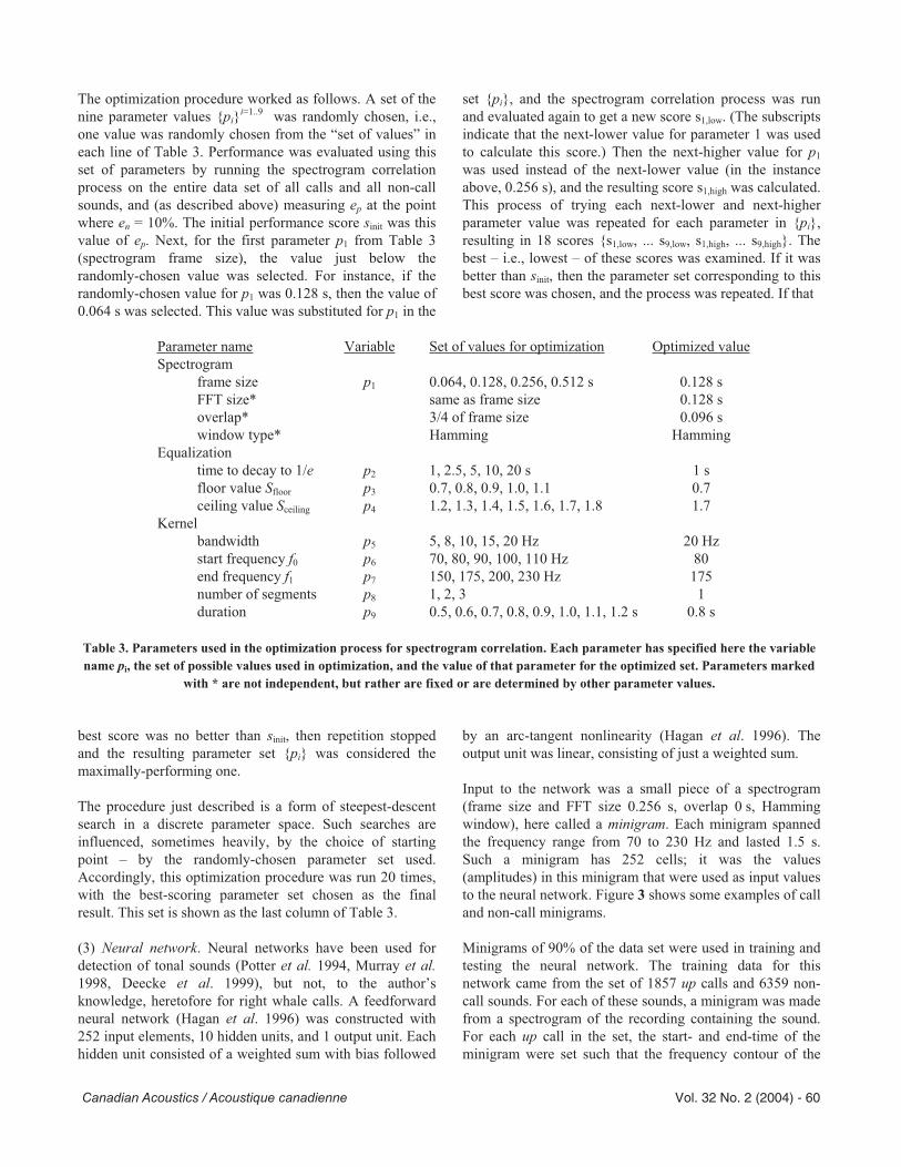
Parameter name Variable Set of values for optimization Optimized valueSpectrogram frame size p1 0.064, 0.128, 0.256, 0.512 s 0.128 s FFT size* same as frame size 0.128 s overlap* 3/4 of frame size 0.096 s window type* Hamming Hamming Equalization time to decay to 1/e p2 1, 2.5, 5, 10, 20 s 1 s floor value Sfloor p3 0.7, 0.8, 0.9, 1.0, 1.1 0.7 ceiling value Sceiling p4 1.2, 1.3, 1.4, 1.5, 1.6, 1.7, 1.8 1.7 Kernel bandwidth p5 5, 8, 10, 15, 20 Hz 20 Hz start frequency f0 p6 70, 80, 90, 100, 110 Hz 80 end frequency f1 p7 150, 175, 200, 230 Hz 175 number of segments p8 1, 2, 3 1 duration p9 0.5, 0.6, 0.7, 0.8, 0.9, 1.0, 1.1, 1.2 s 0.8 s

Table 3. Parameters used in the optimization process for spectrogram correlation. Each parameter has specified here the variablename pi, the set of possible values used in optimization, and the value of that parameter for the optimized set. Parameters marked

with * are not independent, but rather are fixed or are determined by other parameter values.

best score was no better than sinit, then repetition stopped and the resulting parameter set {pi} was considered the maximally-performing one.

The procedure just described is a form of steepest-descent search in a discrete parameter space. Such searches are influenced, sometimes heavily, by the choice of starting point – by the randomly-chosen parameter set used. Accordingly, this optimization procedure was run 20 times, with the best-scoring parameter set chosen as the final result. This set is shown as the last column of Table 3.

(3) Neural network. Neural networks have been used for detection of tonal sounds (Potter et al. 1994, Murray et al.1998, Deecke et al. 1999), but not, to the author’s knowledge, heretofore for right whale calls. A feedforward neural network (Hagan et al. 1996) was constructed with 252 input elements, 10 hidden units, and 1 output unit. Each hidden unit consisted of a weighted sum with bias followed

by an arc-tangent nonlinearity (Hagan et al. 1996). The output unit was linear, consisting of just a weighted sum.

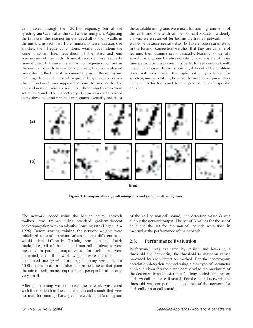
Input to the network was a small piece of a spectrogram (frame size and FFT size 0.256 s, overlap 0 s, Hamming window), here called a minigram. Each minigram spanned the frequency range from 70 to 230 Hz and lasted 1.5 s. Such a minigram has 252 cells; it was the values (amplitudes) in this minigram that were used as input values to the neural network. Figure 3 shows some examples of call and non-call minigrams.

Minigrams of 90% of the data set were used in training and testing the neural network. The training data for this network came from the set of 1857 up calls and 6359 non-call sounds. For each of these sounds, a minigram was made from a spectrogram of the recording containing the sound. For each up call in the set, the start- and end-time of the minigram were set such that the frequency contour of the

Canadian Acoustics / Acoustique canadienne Vol. 32 No. 2 (2004) - 60

call passed through the 120-Hz frequency bin of the spectrogram 0.55 s after the start of the minigram. Adjusting the timing in this manner time-aligned all of the up calls in the minigrams such that if the minigrams were laid atop one another, their frequency contours would occur along the same diagonal line, regardless of the start and end frequencies of the calls. Non-call sounds were similarly time-aligned, but since there was no frequency contour in the non-call sounds to use for alignment, they were aligned by centering the time of maximum energy in the minigram. Training the neural network required target values, values that the network was supposed to learn to produce for the call and non-call minigram inputs. These target values were set at +0.5 and -0.5, respectively. The network was trained using these call and non-call minigrams. Actually not all of

the available minigrams were used for training; one-tenth of the calls and one-tenth of the non-call sounds, randomly chosen, were reserved for testing the trained network. This was done because neural networks have enough parameters, in the form of connection weights, that they are capable of learning their training set – basically, learning to identify specific minigrams by idiosyncratic characteristics of those minigrams. For this reason, it is better to test a network with “new” data absent from its training data set. (This problem does not exist with the optimization procedure for spectrogram correlation, because the number of parameters – nine – is far too small for the process to learn specific calls.)

.

Figure 3. Examples of (a) up call minigrams and (b) non-call minigrams.

The network, coded using the Matlab neural network toolbox, was trained using standard gradient-descent backpropagation with an adaptive learning rate (Hagan et al1996). Before starting training, the network weights were initialized to small random values so that different units would adapt differently. Training was done in “batch mode,” i.e., all of the call and non-call minigrams were presented in parallel, output values for each input were computed, and all network weights were updated. This constituted one epoch of training. Training was done for 5000 epochs in all, a number chosen because at that point the rate of performance improvement per epoch had become very small.

After this training was complete, the network was tested with the one-tenth of the calls and non-call sounds that were not used for training. For a given network input (a minigram

of the call or non-call sound), the detection value D was simply the network output. The set of D values for the set of calls and the set for the non-call sounds were used in measuring the performance of the network.

2.3. Performance Evaluation Performance was evaluated by raising and lowering a threshold and comparing the threshold to detection values produced by each detection method. For the spectrogram correlation detection method using either type of parameter choice, a given threshold was compared to the maximum of the detection function d(t) in a 2 s long period centered on each up call or non-call sound. For the neural network, the threshold was compared to the output of the network for each call or non-call sound.

time

(b)

(a)

61 - Vol. 32 No. 2 (2004) Canadian Acoustics / Acoustique canadienne

For either detection method and for a given threshold, two error measures were determined: the false negative proportion en, which is the proportion of missed calls as a fraction of all calls, and the false positive proportion ep, the proportion of wrongly detected noise sounds as a fraction of all noise sounds. Raising the threshold makes the proportion of false negatives rise and the number of false positives fall, and inversely for lowering the threshold. By varying the threshold between the lowest and highest values produced by any given detection method, one could obtain a parametric curve – the performance curve – detailing the performance of the detection method. Figure 4 shows some examples of such curves. This curve is analogous to the Receiver Operating Characteristic (ROC) curve used in measurement of radar system performance.

A special point on the performance curve was used for comparison of methods. This was the point at which the false-negative proportion en was 10%. The 10% false-negative level was chosen because an up call detection method is probably useful even if it misses 10% of the calls present: Right whales make calls in clusters lasting a few minutes and containing an average of 2 calls (North Atlantic right whales; Matthews et al. 2001) to over an hour and containing 10-15 calls (North Pacific right whales; McDonald and Moore 2002). With a 10% missed-call rate – i.e., a 90% detection rate – and assuming that the probability of detection is independent from one detection to the next, the probability that a detector would miss a cluster ranges from 0.01 down to 10-10 or less. A detector might thus some calls but would be unlikely to miss a whale.

The false-positive proportion ep corresponding to the 10% false-negative point was used as a performance metric, a metric named the single-point score. By choosing this single point on the curve, performance measurement for a given detection method and its configuration parameters was reduced to a single number, enabling direct comparison of disparate methods (and, as explained above, enabling the spectrogram correlation optimization procedure to choose the “best” parameter set).

The performance of any call-detection method depends critically on the signal-to-noise ratio (SNR) of the calls under consideration. The SNR of a given call was characterized as the ratio of the average power during the call in the 50-250 Hz frequency band to the average “noise power,” the power in the 10 s before and 10 s after the call. Note that since this calculation is done before any kind of spectrum equalization, tonal background noise that fluctuates in intensity can make calls that are relatively apparent in a normalized spectrogram have an SNR of 0 dB or even less. The performance curve was calculated separately for calls with SNR <0 dB, calls with SNR from

0-10 dB, calls with SNR from 10-20 dB, and calls with SNR >20 dB.

3. RESULTSThe performance of spectrogram correlation with manually-picked parameters is shown in Fig. 4a. This figure shows a series of parametric performance curves, one curve for each range of call SNRs; each point on this curve corresponds to a certain threshold value, and the (x,y) location plotted is the point (ep, en), i.e., the false-positive vs. false-negative error proportions. In such a plot, the lower-left area is the region of least error and hence of best performance. The single-point score on a given curve may be found by drawing a horizontal line from the 10% mark on the y-axis, seeing where this line intersects the curve, and determining the x-axis value of the intersection. Note that the axes of this plot are logarithmic, so constant ratios are the same size, and small distances on the plot can correspond to relatively large differences in performance. Figure 4b shows the performance curves for spectrogram correlation when the parameters are chosen by the optimization procedure (see also the rightmost column of Table 3), while Fig. 4c shows the curves for the neural network. Figure 4d is a comparison of performance curves for the three detection methods; it was made using all calls regardless of SNR. In this figure, the single-point score is indicated for the neural network (6%) and spectrogram correlation with manually chosen parameters (26%).

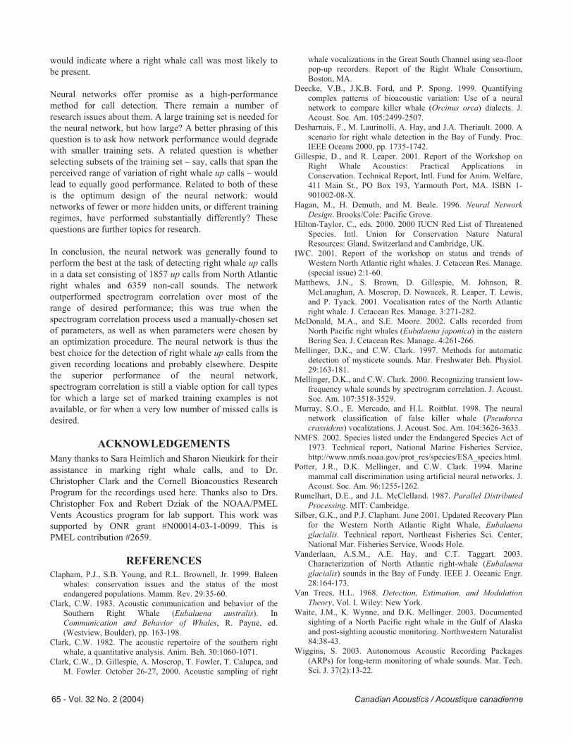
Figure 5 shows some of the calls that resulted in high output values when used as input to the neural network.

4. DISCUSSION As expected, performance of all methods as measured by the ROC curve generally improved with increasing SNR, typically by a factor of 3-6p in going from the calls with SNR less than 0 dB to those with SNR greater than 20 dB. Also note that performance varied only somewhat between the calls with 10-20 dB SNR and those with >20 dB SNR. One reason for this may be that the calls with 10 dB SNR contain as much information as the spectrogram correlation method is able to use; the missed calls may be due to other effects such as odd frequency contours that do not match the usual up call contour.

The performance of the optimized spectrogram correlation method (Fig. 2b, and rightmost column of Table 3) was significantly better than that of spectrogram correlation with manually-chosen parameters. It is not surprising to find a difference, as the optimization procedure used the entire data set to choose its parameters, while the manually-chosen parameters were selected using only a small subset. In addition, the optimization procedure used many days of

Canadian Acoustics / Acoustique canadienne Vol. 32 No. 2 (2004) - 62

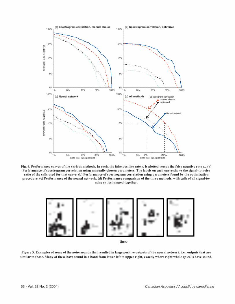
Fig. 4. Performance curves of the various methods. In each, the false positive rate ep is plotted versus the false negative rate en. (a) Performance of spectrogram correlation using manually-chosen parameters. The labels on each curve shows the signal-to-noise ratio of the calls used for that curve. (b) Performance of spectrogram correlation using parameters found by the optimization

procedure. (c) Performance of the neural network. (d) Performance comparison of the three methods, with calls of all signal-to-noise ratios lumped together.

Figure 5. Examples of some of the noise sounds that resulted in large positive outputs of the neural network, i.e., outputs that are similar to those. Many of these have sound in a band from lower left to upper right, exactly where right whale up calls have sound.

time

1% 3% 10% 30% 100% 1%

3%

10%

30%

100%

error rate: false positives

1% 3% 10% 30% 100% 1%

3%

10%

30%

100%

error rate: false positives

1% 3% 10% 30% 100% 1%

3%

10%

30%

100%

error rate: false positives

erro

r ra

te: f

alse

neg

ativ

es

(b) Spectrogram correlation, optimized (a) Spectrogram correlation, manual choice

(d) All methods Spectrogram correlation manual choice optimized

26% 6% 1% 3% 10% 30% 100% 1%

3%

10%

30%

100%

error rate: false positives

erro

r ra

te: f

alse

neg

ativ

es

(c) Neural network

Neural network

63 - Vol. 32 No. 2 (2004) Canadian Acoustics / Acoustique canadienne

computer time (though using a relatively inefficient algorithm), in contrast to the manual method which required only a few hours of the author’s time. However, the degree of difference was surprisingly large, with the optimized method generally performing better by a factor of two to five.

Neural network performance (Fig. 4c) was somewhat better than the optimized spectrogram correlator for calls of poor SNR, though slightly worse for calls of high SNR. Stated another way, the performance curves of the neural network were more closely bunched than those of the optimized spectrogram correlator. This difference may be a reflection of the fact that the neural network had more tunable parameters, and was thus able to adapt to the types of calls – particularly faint calls – and non-call sounds better than the spectrogram correlator. Its range of variation between low-SNR and high-SNR calls was therefore smaller.

The performance curves of Figs. 4a and 4c show anomalies in which the performance for calls of greater SNR was occasionally worse than that for calls lesser SNR. It is not known why this occurred; it may have something to do with the fact that SNR was measured before spectrum equalization, while the methods operate from a spectrogram to which equalization has been applied.

As shown in Fig. 4d, the neural network performed better than either spectrogram correlation method – substantially better than with manually-chosen parameters, and somewhat better than with optimized parameters over most of the range of measurement. There are regions at either end of the curves (the low false-negative and low false-positive ends) at which optimized spectrogram correlation performed slightly better than optimized spectrogram correlation, but in the broad middle range, the neural network was better. This raises the question of whether spectrogram correlation is useful at all. There are three answers to this question:

1) No. The neural network with weights adjusted by the training process described above is plainly the preferred method for detecting the right whale up calls in this data set, and probably for detecting right whale up calls in other data sets.

2) Possibly. One open question is how well the neural network would work for right whales recorded in different locations or at different times of year. This network is optimized for the sounds (both calls and non-call sounds) with which it was trained, but its performance would probably degrade for data collected in a different sonic environment – where, for instance the types of transient interfering sounds were different. Performance of spectrogram correlation would probably degrade too, but it might degrade less, since the spectrogram correlation

process and parameters are less finely tuned to the set of training calls and especially non-noise sounds. Whether this is true is a matter for future research.

3) Yes. The spectrogram correlation method worked reasonably well when its parameters were chosen manually from only a few (20) example calls. Spectrogram correlation may be useful for detecting other call types from right whales, or calls from other animal species. In many cases, a large set of recordings containing thousands of training calls may not exist, or resources may not be available for a person to mark where in the recordings the desired calls are. Having such a set of marked calls is a prerequisite for training a neural network; in the absence of the marked calls, spectrogram correlation may well be a viable option. A single-point score of 26% false detections, as achieved by spectrogram correlation, is quite tolerable for many applications. For instance, if the application is determining whether calls of a certain type occur in a large body of recordings (e.g., Clark et al. 2000, Waite et al. 2003), then using spectrogram correlation with manual choice of parameters could result in detection of most or all of the desired calls, in addition to a small set of undesired non-call sounds. Examining an extra 26% of a small set of detections is almost trivial. In such a case, spectrogram correlation would have worked well.

Another case in which spectrogram correlation might be useful is when minimizing the number of missed calls (false negatives) is the desired. If, for instance, one desired a missed-call rate of 1%, then optimized spectrogram correlation is the best-performing method. Setting the detection threshold for such a missed-call rate would necessarily lead to a large number of false detections (>50% in this case), but that could well be acceptable for some applications. One example is a real-time system for avoiding ship strikes, in which a human operator would check each possible detection before announcing the presence of a right whale. In such a system, the cost of a false detection could be only minimal, but that of a missed detection extremely high.

How would the neural network, which was trained using discrete minigrams, be used in applications such as real-time detection where the signal is continuous in time? The network would be applied once per spectrogram time slice, by extracting the time-frequency portion of the spectrogram – the minigram – that begins at that time slice and has the same frequency bounds and duration as the minigrams used for training. The network would produce an output value for this input minigram; the network's successive output values over time would constitute a detection function, similar to that of Fig. 2b. A threshold could then be applied to this function, and supra-threshold peaks in the detection function

Canadian Acoustics / Acoustique canadienne Vol. 32 No. 2 (2004) - 64

would indicate where a right whale call was most likely to be present.

Neural networks offer promise as a high-performance method for call detection. There remain a number of research issues about them. A large training set is needed for the neural network, but how large? A better phrasing of this question is to ask how network performance would degrade with smaller training sets. A related question is whether selecting subsets of the training set – say, calls that span the perceived range of variation of right whale up calls – would lead to equally good performance. Related to both of these is the optimum design of the neural network: would networks of fewer or more hidden units, or different training regimes, have performed substantially differently? These questions are further topics for research.

In conclusion, the neural network was generally found to perform the best at the task of detecting right whale up calls in a data set consisting of 1857 up calls from North Atlantic right whales and 6359 non-call sounds. The network outperformed spectrogram correlation over most of the range of desired performance; this was true when the spectrogram correlation process used a manually-chosen set of parameters, as well as when parameters were chosen by an optimization procedure. The neural network is thus the best choice for the detection of right whale up calls from the given recording locations and probably elsewhere. Despite the superior performance of the neural network, spectrogram correlation is still a viable option for call types for which a large set of marked training examples is not available, or for when a very low number of missed calls is desired.

ACKNOWLEDGEMENTS Many thanks to Sara Heimlich and Sharon Nieukirk for their assistance in marking right whale calls, and to Dr. Christopher Clark and the Cornell Bioacoustics Research Program for the recordings used here. Thanks also to Drs. Christopher Fox and Robert Dziak of the NOAA/PMEL Vents Acoustics program for lab support. This work was supported by ONR grant #N00014-03-1-0099. This is PMEL contribution #2659.

REFERENCES Clapham, P.J., S.B. Young, and R.L. Brownell, Jr. 1999. Baleen

whales: conservation issues and the status of the most endangered populations. Mamm. Rev. 29:35-60.

Clark, C.W. 1983. Acoustic communication and behavior of the Southern Right Whale (Eubalaena australis). In Communication and Behavior of Whales, R. Payne, ed. (Westview, Boulder), pp. 163-198.

Clark, C.W. 1982. The acoustic repertoire of the southern right whale, a quantitative analysis. Anim. Beh. 30:1060-1071.

Clark, C.W., D. Gillespie, A. Moscrop, T. Fowler, T. Calupca, and M. Fowler. October 26-27, 2000. Acoustic sampling of right

whale vocalizations in the Great South Channel using sea-floor pop-up recorders. Report of the Right Whale Consortium, Boston, MA.

Deecke, V.B., J.K.B. Ford, and P. Spong. 1999. Quantifying complex patterns of bioacoustic variation: Use of a neural network to compare killer whale (Orcinus orca) dialects. J. Acoust. Soc. Am. 105:2499-2507.

Desharnais, F., M. Laurinolli, A. Hay, and J.A. Theriault. 2000. A scenario for right whale detection in the Bay of Fundy. Proc. IEEE Oceans 2000, pp. 1735-1742.

Gillespie, D., and R. Leaper. 2001. Report of the Workshop on Right Whale Acoustics: Practical Applications in Conservation. Technical Report, Intl. Fund for Anim. Welfare, 411 Main St., PO Box 193, Yarmouth Port, MA. ISBN 1-901002-08-X.

Hagan, M., H. Demuth, and M. Beale. 1996. Neural Network Design. Brooks/Cole: Pacific Grove.

Hilton-Taylor, C., eds. 2000. 2000 IUCN Red List of Threatened Species. Intl. Union for Conservation Nature Natural Resources: Gland, Switzerland and Cambridge, UK.

IWC. 2001. Report of the workshop on status and trends of Western North Atlantic right whales. J. Cetacean Res. Manage. (special issue) 2:1-60.

Matthews, J.N., S. Brown, D. Gillespie, M. Johnson, R. McLanaghan, A. Moscrop, D. Nowacek, R. Leaper, T. Lewis, and P. Tyack. 2001. Vocalisation rates of the North Atlantic right whale. J. Cetacean Res. Manage. 3:271-282.

McDonald, M.A., and S.E. Moore. 2002. Calls recorded from North Pacific right whales (Eubalaena japonica) in the eastern Bering Sea. J. Cetacean Res. Manage. 4:261-266.

Mellinger, D.K., and C.W. Clark. 1997. Methods for automatic detection of mysticete sounds. Mar. Freshwater Beh. Physiol. 29:163-181.

Mellinger, D.K., and C.W. Clark. 2000. Recognizing transient low-frequency whale sounds by spectrogram correlation. J. Acoust. Soc. Am. 107:3518-3529.

Murray, S.O., E. Mercado, and H.L. Roitblat. 1998. The neural network classification of false killer whale (Pseudorcacrassidens) vocalizations. J. Acoust. Soc. Am. 104:3626-3633.

NMFS. 2002. Species listed under the Endangered Species Act of 1973. Technical report, National Marine Fisheries Service, http://www.nmfs.noaa.gov/prot_res/species/ESA_species.html.

Potter, J.R., D.K. Mellinger, and C.W. Clark. 1994. Marine mammal call discrimination using artificial neural networks. J. Acoust. Soc. Am. 96:1255-1262.

Rumelhart, D.E., and J.L. McClelland. 1987. Parallel Distributed Processing. MIT: Cambridge.

Silber, G.K., and P.J. Clapham. June 2001. Updated Recovery Plan for the Western North Atlantic Right Whale, Eubalaena glacialis. Technical report, Northeast Fisheries Sci. Center, National Mar. Fisheries Service, Woods Hole.

Vanderlaan, A.S.M., A.E. Hay, and C.T. Taggart. 2003. Characterization of North Atlantic right-whale (Eubalaenaglacialis) sounds in the Bay of Fundy. IEEE J. Oceanic Engr. 28:164-173.

Van Trees, H.L. 1968. Detection, Estimation, and Modulation Theory, Vol. I. Wiley: New York.

Waite, J.M., K. Wynne, and D.K. Mellinger. 2003. Documented sighting of a North Pacific right whale in the Gulf of Alaska and post-sighting acoustic monitoring. Northwestern Naturalist 84:38-43.

Wiggins, S. 2003. Autonomous Acoustic Recording Packages (ARPs) for long-term monitoring of whale sounds. Mar. Tech. Sci. J. 37(2):13-22.

65 - Vol. 32 No. 2 (2004) Canadian Acoustics / Acoustique canadienne