A COMPARATIVE STUDY ON DIRECT ANALYSIS · PDF fileÇelik yapılar için stabilite...
153
A COMPARATIVE STUDY ON DIRECT ANALYSIS METHOD AND EFFECTIVE LENGTH METHOD IN ONE-STORY SEMI-RIGID FRAMES A THESIS SUBMITTED TO THE GRADUATE SCHOOL OF NATURAL AND APPLIED SCIENCES OF MIDDLE EAST TECHNICAL UNIVERSITY BY AFŞİN EMRAH DEMİRTAŞ IN PARTIAL FULFILLMENT OF THE REQUIREMENTS FOR THE DEGREE OF MASTER OF SCIENCE IN CIVIL ENGINEERING SEPTEMBER 2012
Transcript of A COMPARATIVE STUDY ON DIRECT ANALYSIS · PDF fileÇelik yapılar için stabilite...

A COMPARATIVE STUDY ON DIRECT ANALYSIS METHOD AND EFFECTIVE LENGTH METHOD IN ONE-STORY SEMI-RIGID FRAMES
A THESIS SUBMITTED TO THE GRADUATE SCHOOL OF NATURAL AND APPLIED SCIENCES
OF MIDDLE EAST TECHNICAL UNIVERSITY
BY
AFŞİN EMRAH DEMİRTAŞ
IN PARTIAL FULFILLMENT OF THE REQUIREMENTS FOR
THE DEGREE OF MASTER OF SCIENCE IN
CIVIL ENGINEERING
SEPTEMBER 2012

Approval of the thesis:
A COMPARATIVE STUDY ON DIRECT ANALYSIS METHOD AND EFFECTIVE LENGTH METHOD IN ONE-STORY SEMI-RIGID FRAMES
Submitted by AFŞİN EMRAH DEMİRTAŞ in partial fulfillment of the requirements for the degree of Master of Science in Civil Engineering Department, Middle East Technical University by, Prof. Dr. Canan Özgen ____________________ Dean, Graduate School of Natural and Applied Sciences Prof. Dr. Güney Özcebe ____________________ Head of Department, Civil Engineering Prof. Dr. Uğurhan Akyüz ____________________ Supervisor, Civil Engineering Dept., METU Examining Committee Members: Prof. Dr. Çetin Yılmaz _____________________ Civil Engineering Dept., METU Prof. Dr. Uğurhan Akyüz _____________________ Civil Engineering Dept., METU Prof. Dr. Cem Topkaya _____________________ Civil Engineering Dept., METU Assoc. Prof. Dr. Alp Caner _____________________ Civil Engineering Dept., METU Halit Levent Akbaş, M.S. _____________________ Chairman of Board, ATAK Engineering Date: Sep 6, 2012

iii
I hereby declare that all information in this document has been obtained and presented in accordance with academic rules and ethical conduct. I also declare that, as required by these rules and conduct, I have fully cited and referenced all material and results that are not original to this work.
Name, Last name: Afşin Emrah DEMİRTAŞ
Signature :

iv
ABSTRACT
A COMPARATIVE STUDY ON DIRECT ANALYSIS METHOD AND EFFECTIVE LENGTH METHOD IN ONE-STORY SEMI-RIGID FRAMES
Demirtaş, Afşin Emrah
M.S., Department of Civil Engineering
Supervisor: Prof. Dr. Uğurhan Akyüz
September 2012, 135 pages
For steel structures, stability is a very important concept since many steel structures
are governed by stability limit states. Therefore, stability of a structure should be
assessed carefully considering all parameters that affect the stability of the structure.
The most important of these parameters can be listed as geometric imperfections,
member inelasticity and connection rigidity. Geometric imperfections and member
inelasticity are taken into account with the stability method used in the design. At
this point, the stability methods gain importance. The Direct Analysis Method, the
default stability method in 2010 AISC Specification, is a new, more transparent and
more straightforward method, which captures the real structure behavior better than
Effective Length Method. In this thesis, a study has been conducted on the semi-rigid
steel frames to compare Direct Analysis Method and Effective Length Method and to
investigate the effect of flexible connections to stability. Four frames are designed
for different connection rigidities with stability methods existing in the 2010 AISC
Specification: Direct Analysis Method and Effective Length Method. At the end,

v
conclusions are drawn about the comparison of these two stability methods and the
effect of semi-rigid connections to stability.
Keywords: Direct Analysis Method, Effective Length Method, Semi-Rigid Frames,
Frame Stability

vi
ÖZ
DİREKT ANALİZ METODU İLE EFEKTİF UZUNLUK METODUNUN TEK KATLI YARI RİJİT BAĞLANTILI ÇERÇEVELERDE KARŞILAŞTIRILMASI
Demirtaş, Afşin Emrah
Yüksek Lisans, İnşaat Mühendisliği Bölümü
Tez Yöneticisi: Prof. Dr. Uğurhan Akyüz
Eylül 2012, 135 sayfa
Çelik yapılar için stabilite kavramı çok önemlidir çünkü çoğu çelik yapı stabilite
limit durumlarına göre tasarlanmaktadır. Bundan dolayı, bir yapının stabilitesi onu
etkileyebilecek bütün parametreler göz önünde bulundurularak itinayla
değerlendirilmelidir. Geometrik kusurlar, elemanların inelastisitesi ve bağlantı
rijitliği bu parametrelerin en önemlileridirler. Geometrik kusurlar ve eleman
inelastisiteleri tasarım esnasında kullanılan stabilite metodu ile değerlendirilirler. Bu
noktada stabilite metotları önem kazanmaktadır. 2010 AISC şartnamesinde geçerli
stabilite metodu olan Direkt Analiz Metodu yeni, daha şeffaf ve daha dolambaçsız
bir metot olup Efektif Uzunluk Metodu’na göre gerçek yapı davranışını daha iyi
yansıtmaktadır. Bu tezde, Direk Analiz Metodu ile Efektif Uzunluk Metodunu
karşılaştırmak ve esnek bağlantıların stabiliteye etkisini incelemek için yarı rijit çelik
çerçeveler üzerine bir çalışma yapılmıştır. 2010 AISC şartnamesinde mevcut olan
stabilite metotları (Direkt Analiz ve Efektif Uzunluk Metotları) kullanılarak değişik
bağlantı rijitlikleri ile dört tane çelik çerçeve tasarlanacaktır. En sonda, bu iki

vii
metodun kıyaslanması ve yarı rijit bağlantıların stabiliteye etkisi üzerine sonuçlar
çıkartılacaktır.
Anahtar Kelimeler: Direkt Analiz Metodu, Efektif Uzunluk Metodu, Yarı Rijit
Çerçeveler, Çerçevelerin Stabilitesi

viii
To My Family

ix
ACKNOWLEDGMENT
The author wishes to express his deepest gratitude to his supervisor Prof.Dr. Uğurhan
Akyüz for his guidance, careful supervision, criticisms, patience and insight throughout
the research.
My special thanks go to Mehmet Akın Çetinkaya, Eren Güler, Merve Zayim, Ezgi
Toplu Demirtaş, Alper Demirtaş and Ali Demirtaş for their support and the
motivation they provided to me.
My deepest gratitude goes to my mother Yurdagül Demirtaş and my father Eşref
Demirtaş for their constant support and encouragement. This thesis would not have
been possible without them.
The author wishes to thank in particular all those people whose friendly assistance and
wise guidance supported him throughout the research.
I also thank to TÜBİTAK for providing me financial support during my Master’s
thesis.

x
TABLE OF CONTENTS
ABSTRACT ............................................................................................................... IV
ÖZ .............................................................................................................................. VI
ACKNOWLEDGMENT ............................................................................................ IX
TABLE OF CONTENTS ............................................................................................ X
LIST OF TABLES .................................................................................................... XII
LIST OF FIGURES ................................................................................................ XIII
LIST OF SYMBOLS / ABBREVATIONS ............................................................. XV
CHAPTER
1. INTRODUCTION ............................................................................................... 1
1.1. MOTIVATION .............................................................................................. 1
1.2. LITERATURE SURVEY ................................................................................ 2
1.3. OBJECT AND SCOPE ................................................................................... 4
2. THEORY ............................................................................................................. 7
2.1. DIRECT ANALYSIS METHOD ..................................................................... 7
2.2. EFFECTIVE LENGTH METHOD................................................................. 12
2.2.1.Introduction .......................................................................................... 12
2.2.2.Buckling Analysis of Semi-Rigid Frames ............................................ 12
2.2.3.AISC 360-10 Requirements ................................................................. 14
2.3. ANALYSIS OF SEMI-RIGID FRAMES ........................................................ 16
2.3.1.Introduction .......................................................................................... 16
2.3.2.Types of Semi-Rigid Connections ....................................................... 17
2.3.3.Behavior and Modeling of Connections ............................................... 22
2.3.4.Analysis of Semi-Rigid Frames ........................................................... 24
2.4. APPROXIMATE SECOND-ORDER ANALYSIS .......................................... 28
3. CASE STUDIES ............................................................................................... 32
3.1. GENERAL INFORMATION AND ASSUMPTIONS ..................................... 32
3.2. CASE STUDY – I ......................................................................................... 37
3.2.1.Design with Effective Length Method ................................................. 38
3.2.2.Design with Direct Analysis Method ................................................... 48

xi
3.3. CASE STUDY – II ........................................................................................ 53
3.3.1.Design with Effective Length Method ................................................. 54
3.3.2.Design with Direct Analysis Method ................................................... 56
3.4. CASE STUDY – III ...................................................................................... 59
3.4.1.Design with Effective Length Method ................................................. 60
3.4.2.Design with Direct Analysis Method ................................................... 62
3.5. CASE STUDY – IV ...................................................................................... 65
3.5.1.Design with Effective Length Method ................................................. 66
3.5.2.Design with Direct Analysis Method ................................................... 71
4. RESULTS AND DISCUSSIONS OF RESULTS ............................................. 76
4.1. RESULTS .................................................................................................... 76
4.1.1.Results of Case - I ................................................................................ 77
4.1.2.Results of Case - II ............................................................................... 79
4.1.3.Results of Case - III .............................................................................. 81
4.1.4.Results of Case - IV .............................................................................. 83
4.2. DISCUSSION OF RESULTS ........................................................................ 87
5. CONCLUSIONS AND FUTURE RECOMMENDATIONS ........................... 93
5.1. CONCLUSIONS .......................................................................................... 93
5.2. FUTURE RECOMMENDATIONS ............................................................... 96
REFERENCES ........................................................................................................... 97
APPENDICES
A. FLEXURAL STRENGTH OF COLUMNS. ........................................................ 100
B. COMPRESSIVE STRENGTH OF COLUMNS ................................................... 106
C. STRUCTURAL ANALYSIS STEPS OF CASES ................................................ 112
D. LATERAL DRIFT VALUES OF CASES .......................................................... 132
xii
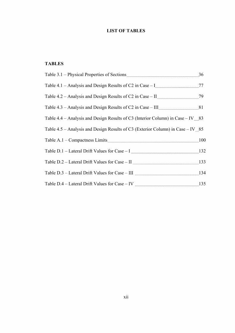
LIST OF TABLES
TABLES Table 3.1 – Physical Properties of Sections 36 Table 4.1 – Analysis and Design Results of C2 in Case – I 77 Table 4.2 – Analysis and Design Results of C2 in Case – II 79 Table 4.3 – Analysis and Design Results of C2 in Case – III 81 Table 4.4 – Analysis and Design Results of C3 (Interior Column) in Case – IV 83 Table 4.5 – Analysis and Design Results of C3 (Exterior Column) in Case – IV 85 Table A.1 – Compactness Limits 100 Table D.1 – Lateral Drift Values for Case – I 132 Table D.2 – Lateral Drift Values for Case – II 133 Table D.3 – Lateral Drift Values for Case – III 134 Table D.4 – Lateral Drift Values for Case – IV 135
xiii
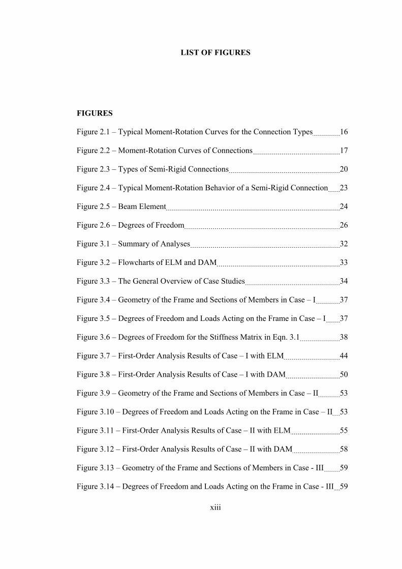
LIST OF FIGURES
FIGURES Figure 2.1 – Typical Moment-Rotation Curves for the Connection Types 16 Figure 2.2 – Moment-Rotation Curves of Connections 17 Figure 2.3 – Types of Semi-Rigid Connections 20 Figure 2.4 – Typical Moment-Rotation Behavior of a Semi-Rigid Connection 23 Figure 2.5 – Beam Element 24 Figure 2.6 – Degrees of Freedom 26 Figure 3.1 – Summary of Analyses 32 Figure 3.2 – Flowcharts of ELM and DAM 33 Figure 3.3 – The General Overview of Case Studies 34 Figure 3.4 – Geometry of the Frame and Sections of Members in Case – I 37 Figure 3.5 – Degrees of Freedom and Loads Acting on the Frame in Case – I 37 Figure 3.6 – Degrees of Freedom for the Stiffness Matrix in Eqn. 3.1 38 Figure 3.7 – First-Order Analysis Results of Case – I with ELM 44 Figure 3.8 – First-Order Analysis Results of Case – I with DAM 50 Figure 3.9 – Geometry of the Frame and Sections of Members in Case – II 53 Figure 3.10 – Degrees of Freedom and Loads Acting on the Frame in Case – II 53 Figure 3.11 – First-Order Analysis Results of Case – II with ELM 55 Figure 3.12 – First-Order Analysis Results of Case – II with DAM 58 Figure 3.13 – Geometry of the Frame and Sections of Members in Case - III 59 Figure 3.14 – Degrees of Freedom and Loads Acting on the Frame in Case - III 59

xiv
Figure 3.15 – First-Order Analysis Results of Case – III with ELM 61 Figure 3.16 – First-Order Analysis Results of Case – III with DAM 64 Figure 3.17 – Geometry of the Frame and Sections of Members in Case - IV 65 Figure 3.18 – Degrees of Freedom and Loads Acting on the Frame in Case - IV 66 Figure 3.19 – First-Order Analysis Results of Case – IV with ELM 67 Figure 3.20 – The Stiffness Matrix of the System in Case – IV with ELM 68 Figure 3.21 – The Stiffness Matrix of the System for Buckling Analysis in
Case – IV with ELM 70 Figure 3.22 – First-Order Analysis Results of Case – IV with DAM 72 Figure 3.23 – The Stiffness Matrix of the System in Case – IV with DAM 73 Figure 4.1 – Demand/Capacity vs. End-Rigidity for Case – I 78 Figure 4.2 – Demand/Capacity vs. End-Rigidity for Case – II 80 Figure 4.3 – Demand/Capacity vs. End-Rigidity for Case – III 82 Figure 4.4 - Demand/Capacity vs. End-Rigidity for C3 in Case – IV 84 Figure 4.5 - Demand/Capacity vs. End-Rigidity for C4 in Case – IV 86 Figure A.1 – Moment Values for Cb Calculation 103

xv
LIST OF SYMBOLS / ABBREVATIONS
A Cross-sectional area (m2)
Ag Gross cross-sectional area of member (m2)
AISC American Institute of Steel Construction
AISC 360-05 2005 AISC Specification for Structural Steel Buildings
AISC 360-10 2010 AISC Specification for Structural Steel Buildings
ASD Allowable stress design
B1 Multiplier to account for P-δ
B2 Multiplier to account for P-∆
Cb Lateral-torsional buckling modification factor for non-uniform
moment diagrams
Cm Coefficient accounting for non-uniform moment
Cw Warping constant (m6)
D Displacement matrix of the system
DAM Direct analysis method
D/C Demand/capacity ratio
E Modulus of elasticity (MPa)
ELM Effective length factor
Fe Elastic buckling stress (MPa)
Fy Minimum yield stress (MPa)
H Story shear, in the direction of translation being considered,
produced by the lateral forces used to compute ∆H (N)
I Moment of inertia in the plane of bending (m4)
Ix Moment of inertia in x-direction (m4)
Iy Moment of inertia in y-direction (m4)
J Torsional constant (m4)
K Effective length factor
K Stiffness matrix of the system
Kx Effective length factor for flexural buckling about x-axis

xvi
Ky Effective length factor for flexural buckling about y-axis
K1 Effective length factor in the plane of bending, calculated
based on the assumption of no lateral translation at the member
ends
L Length of member (m)
LRFD Load and resistance factor design
Lb Length between points that are either braced against lateral
displacement of compression flange or braced against twist of
the cross-section (m)
Lp Limiting laterally unbraced length for the limit state of
yielding (m)
Lr Limiting laterally unbraced length for the limit state of
inelastic lateral-torsional buckling (m)
MA End moment at joint A (N·m)
MB End moment at joint B (N·m)
Mc Available flexural strength
Mlt First-order moment due to lateral translation of the structure
only (N·m)
Mnt First-order moment with the structure restrained against lateral
translation (N·m)
M1 Smaller moment at end of unbraced length (N·m)
M2 Larger moment at end of unbraced length (N·m)
Ni Notional load applied at ith level (N)
Pc Available axial strength (N)
Pcr Critical buckling load (N)
Pe Elastic critical buckling load (N)
Pe1 Elastic critical buckling strength of the member in the plane of
bending (N)
Plt First-order axial force with the structure restrained against
lateral translation (N)
Pmf Total vertical load in columns in the story that are part of
moment frames (N)

xvii
Pn Nominal axial strength (N)
Pnt First-order axial force due to lateral translation of the structure
only (N)
Pr Required axial compressive strength (N)
Pestory Elastic critical buckling strength for the story in the direction
of translation being considered (N)
Pstory Total vertical load supported by the story including loads in
columns that are not part of the lateral force resisting system
(N)
Py Axial yield strength (N)
Q Force vector of the system
RkiA Initial stiffness of rotational spring at joint A (N·m)
RkiB Initial stiffness of rotational spring at joint B (N·m)
RM Coefficient to account for influence of P-δ and P-∆
Sx Section modulus about x-axis (m3)
Sy Section modulus about y-axis (m3)
Yi Gravity load applied at ith level (N)
Zx Plastic section modulus about x-axis (m3)
Zy Plastic section modulus about y-axis (m3)
b Width of the flange (m)
db Displacement matrix of the beam
dc Displacement matrix of the column
h Total depth of the cross-section (m)
ho Distance between the flange centroids (m)
kb Stiffness matrix of the beam
kc Stiffness matrix of the column
r Radius of gyration (m) [Eqn. 2.4]
r End-fixity ratio [Eqn. 2.20]
rx Radius of gyration in x-direction (m)
ry Radius of gyration in y-direction (m)
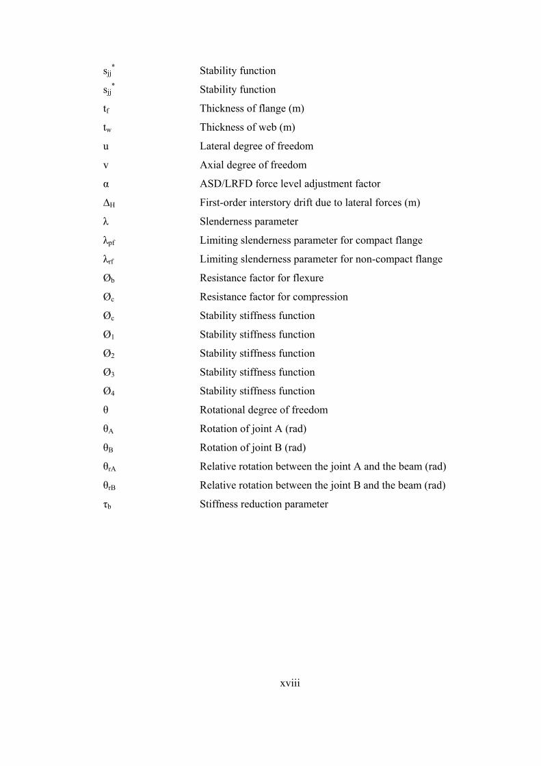
sii* Stability function
sij* Stability function
xviii
sjj* Stability function
sjj* Stability function
tf Thickness of flange (m)
tw Thickness of web (m)
u Lateral degree of freedom
v Axial degree of freedom
α ASD/LRFD force level adjustment factor
∆H First-order interstory drift due to lateral forces (m)
λ Slenderness parameter
λpf Limiting slenderness parameter for compact flange
λrf Limiting slenderness parameter for non-compact flange
Øb Resistance factor for flexure
Øc Resistance factor for compression
Øc Stability stiffness function
Ø1 Stability stiffness function
Ø2 Stability stiffness function
Ø3 Stability stiffness function
Ø4 Stability stiffness function
θ Rotational degree of freedom
θA Rotation of joint A (rad)
θB Rotation of joint B (rad)
θrA Relative rotation between the joint A and the beam (rad)
θrB Relative rotation between the joint B and the beam (rad)
τb Stiffness reduction parameter

1
CHAPTER 1
INTRODUCTION
1.1. MOTIVATION
Stability is a very important concept for steel structures since most steel structures
are governed by stability limit states. Local instability, such as compression flange
buckling, and member instability, such as buckling of a column, may lead the
structure to collapse. Therefore, stability provisions of steel design specifications are
continuously improved to capture the real structure behavior and so to minimize the
destabilizing effects.
In the Appendix 7 of 2005 AISC Specification for Structural Steel Buildings (AISC
360-05), Direct Analysis Method (DAM) was first introduced as an alternative to the
Effective Length Method (ELM). Then in 2010 AISC Specification for Structural
Steel Buildings (AISC 360-10) it became the default stability design method as it is
given in Chapter C.
The need to develop a new method is the drawbacks of the ELM. These drawbacks
can be listed as:
ELM is based on many assumptions, which are hardly satisfied in a real
structure. Inconsistencies between the assumptions and the real structure
behavior lead to wrong estimation of internal forces and moments.
ELM underestimates the internal forces and moments, due to this reason
ELM cannot be used for structures having drift-ratio greater than 1.5 that
means ELM is not applicable to all structures.

2
Geometric imperfections and member inelasticity are not accounted for in the
analysis instead they are accounted for in the resistance terms that causes
misinterpretation of both analysis results and member strengths.
On the other hand, DAM is a more straightforward, transparent and accurate stability
design method. It considers member inelasticity and geometric imperfections in the
analysis and it calculates compressive strength of members with an effective length
factor equals to 1.00. Therefore, the DAM captures the real structure behavior better
than the ELM and it provides the designer a simpler and straightforward stability
design procedure.
To obtain realistic analysis results, the stability method used in the analysis is
important along with the realistic modeling of the structure. With the help of
advanced commercial software, detailed 3-D modeling of structures is possible.
However, there is still an important idealization in modeling that makes the structural
model away from the real structure behavior: connections.
Steel frames are designed under the assumption that the beam-to-column connection
is either fully rigid or ideally pinned. However in reality, any connection is neither
fully rigid nor ideally pinned. Connection rigidity has an influence on the internal
force distribution of the system and lateral drift of the structure. Therefore,
connection rigidity should be modeled such that it reflects the connection behavior.
1.2. LITERATURE SURVEY
In this section, the researches conducted on comparison of ELM and DAM and the
researches carried out with semi-rigid frames are discussed.
Ziemian et al [1] investigated eleven two-and-three-dimensional structural systems to
evaluate and compare ELM and DAM. Also advanced-second order inelastic

3
analyses were used to assess the adequacy of all design methods. They concluded
that ELM and DAM provide similar results and for beam-columns subjected to
minor-axis bending DAM is slightly unconservative.
In the study of Surovek et al [2], an 11-bay single-story frame was studied to discuss
the three design approaches (Direct Analysis Method, Effective Length Method and
Advanced Analysis) for the assessment of frame stability. The primary attribute of
this frame was that it is sensitive to initial imperfection effects. To illustrate
distinctive features of the design approaches, large gravity loads were applied to
produce significant P-∆ effects. They concluded that axial forces are similar in each
method but the internal moments differ substantially. ELM underestimates the
internal moments since the moments in the frame are highly sensitive to out-of-
plumbness of the structure which is not directly considered in the analysis with ELM,
and DAM is conservative when calculating the internal moments since the columns
are elastic at the factored load although the stiffnesses are reduced due to inelasticity.
In his study, Prajzner [3] dealt with the evaluation of case studies including a portal
frame, a leaning column frame, a multi-story structure, and a multi-bay frame in
order to assess the adequacy of ELM and DAM. To provide a reasonable
representation of real frame behavior second-order plastic analysis approach was
used as the third method and the results obtained with this method were treated as
real results. In this study, ELM produced unsafe designs in structures where second-
order effects are significant. On the other hand, DAM produced overly conservative
designs for the same type of structures. He suggested a “sway” factor to quantify the
second-order effects. The intent of the “sway” factor is to calibrate the results of
ELM and DAM in structures where the second-order effects are significant.
Surovek et al [4] presented an approach that allows for the consideration of non-
linear connection using commonly available elastic analysis software. The partially
restrained frames were analyzed using Direct Analysis Method. The aim of the
proposed connection approach was to simplify the consideration non-linear

4
connection response in the analysis of partially restrained frames. By using Direct
Analysis Method, they intended to simplify also the strength assessment of the
structure by eliminating the calculation of effective length factor. In this study, the
proposed method for handling the connection non-linearity along with the Direct
Analysis Method have been shown to make it simpler to obtain realistic distribution
of internal forces in partially restrained frames.
Kartal et al [5] developed a finite element program SEMIFEM in FORTRAN
language to perform structural analysis that considers semi-rigid connections. The
aim of their study was to investigate the effect of semi-rigid connections on the
structure behavior. In their study, they adopted the formula suggested by Monforton
and Wu [6] to define the connection stiffness in terms of the connection stiffness-
beam stiffness ratio.
The formula suggested by Monforton and Wu [6] was also adopted by Xu [7] in his
study on calculation of critical buckling loads of semi-rigid steel frames and by
Patodi et al [8] in their study on first order analysis of plane frames with semi-rigid
connections. They used this formula to define the stiffness of the connection in terms
of the stiffness of the beam that the connection is attached to.
1.3. OBJECT AND SCOPE
Before development of DAM, ELM was the common stability method that has been
used widely by many engineers. However ELM is based on some assumptions which
are hardly satisfied in real structures and it has many drawbacks which make stability
design very complex and challenging in some cases. DAM was developed and
presented in the latest version of AISC Specification for Steel Structures to
compensate the drawbacks of ELM and to make stability design easier and more
straightforward for engineers. A number of studies were conducted to compare DAM
5
and ELM in order to investigate whether DAM is a more straightforward method and
superior to ELM.
In this study, DAM and ELM are compared in one-story semi-rigid frames. The
objective of this study is to compare the two stability methods in semi-rigid frames
and to investigate the influence of connection rigidity on the stability of the frame.
Four frames are used as case studies: first three ones are one-story one-bay frames
consisting of two columns and one beam where the columns are oriented such that
they are in major-axis bending. The only difference between these three frames is the
loads. In the first frame, horizontal load is the highest but the axial load is the lowest
and in the third frame, horizontal load is the lowest whereas the axial load is the
highest. The aim in selecting these three frames is to investigate the load effects on
the stability methods. The fourth frame is a one-story three-bay frame consisting of
two columns in major-axis bending, two columns in minor-axis bending and three
beams. The aim in selecting the fourth frame, where the some of the columns are in
minor-axis bending, is to investigate the influence of column orientation on stability
methods. The beams in all cases are connected to the columns with semi-rigid
connections. The frames are analyzed with different stiffness values of semi-rigid
connections and with both stability methods. At the end, critical columns in each
case are designed according to the AISC 360-10 and demand/capacity ratios of
columns are obtained for different connection stiffnesses and for both DAM and
ELM. The conclusion part of the study deals with these demand/capacity ratios.
This study is composed of five chapters. In first chapter, an introduction part exists
which gives a general information about the study, a brief background for the DAM
along with semi-rigid frames and the aim of the study. In second chapter, the theory
of methods, which are used in third chapter, are given and explained. These are
Direct Analysis Method, Effective Length Method, Analysis of Semi-Rigid Frames
and Approximate Second-Order Analysis. The analysis of frames and the design of
columns are given in third chapter. The results of the analyses and designs in the

6
third chapter and the discussions related to the results are given in fourth chapter.
The last chapter, Chapter 5, contains conclusion of the study and future
recommendations.
7
CHAPTER 2
THEORY
2.1. DIRECT ANALYSIS METHOD
Direct Analysis Method (DAM) was first introduced in 2005 version of the AISC
Specification for Structural Steel Buildings as an alternative method to the Effective
Length Method (ELM) and First-Order Analysis Method. Then in 2010 version of
the specification, it became the standard stability design method as it is addressed in
Chapter C. DAM has many advantages, such as; it obtains the analysis results more
accurately and realistic, it is applicable to all type of structures and it eliminates the
calculation of K factor.
ELM neglects initial imperfections and inelasticity during analysis and
underestimates member demand. To compensate this underestimate, it requires the
use of K factor to decrease the member capacity. Therefore, in ELM, the forces and
capacities obtained do not reflect the real behavior of the structure. In DAM, initial
imperfections and inelasticity are considered during the analysis and this eliminates
the need for the K factor. Thus, DAM results in a design which is very close to the
real structure behavior.
DAM is the most applicable method among all stability methods. It can be used for
all types of steel structures such as braced frames, moment frames and combined
systems without any limitation. The ratio of second-order drift to first-order drift
shall be equal to or less than 1.5 in ELM however there is no such a limitation in
DAM.

8
The biggest advantage that DAM provides is the elimination of K factor calculation.
In ELM, the analysis is performed with neglecting the geometric imperfections and
inelasticity and they are accounted for in member capacity calculations with
increasing the K factor. In DAM, geometric imperfections and inelasticity are
included in the analysis therefore the need to calculate the K factor is unnecessary
and it can be taken as 1.0 for all members.
Since DAM has many advantages, it is expected that there are too many
sophisticated requirements however the requirements of DAM are simple and easy to
apply. There are three main requirements of DAM which are;
1. A rigorous second-order analysis including both P-Δ and P-δ effects should
be conducted. Use of approximate methods is also permitted.
2. The effect of initial imperfections should be taken into account. The out-of-
plumbness of columns can be directly modeled by displacing the points of
intersection of members from their nominal locations or notional loads can
be used.
3. Reduced stiffness of members should be used in the analysis. This reduction
accounts for system reliability (uncertainty in stiffness and strength) and
inelasticity.
Second-Order Analysis
To reflect a real structure behavior, a rigorous second-order analysis considering
both P-Δ and P-δ effects should be conducted. It is also acceptable to obtain second-
order results by an approximate method given in Appendix 8 of the AISC 360-10. In
this alternative and approximate method there are two multipliers; B1 and B2. By
applying these multipliers to the results of a first-order analysis an approximate
second-order solution may be obtained. This method will be explained in details in
Section 2.4.

9
L
L/500
Initial Imperfections
The effect of out-of-plumbness of columns should be taken into account by
considering the initial imperfections in the intersection of members. These
imperfections can be directly modeled by displacing the intersection of members
from their nominal locations or can be represented by notional loads. The notional
loads at each level of the structure are calculated as;
0.002 · · 2.1
where α = 1.0 for LRFD and 1.6 for ASD Ni = notional load applied at ith level (N) Yi = gravity load applied at ith level (N)
The notional load coefficient 0.002 is based on a nominal
initial out-of-plumbness ratio of L/500 which is the maximum
tolerance on column plumbness specified in the AISC Code of
Standard Practice.
Y3
Y2
Y1
N3
N2
N1

10
If the second-order drift to first-order drift ratio is smaller than or equal to 1.7, it is
not obligatory to use notional loads in a load combination which includes other
lateral loads.
Reduced Stiffness
After rolling or welding process, the cross-section of the steel member begins to
cool. First the extreme fibers of the section cool, then the remaining portions of the
section cool. When the remaining portions cool, their contraction is prevented by
extreme fibers that have already cooled. This results in development of tensile and
compressive stresses in the cross-section. When a compressive force is applied to this
cross-section, yielding will first occur in the portions of the section which are under
compressive residual stress. Therefore, the spread of plasticity in the cross-section is
affected by the presence of residual stress [9]. To account for geometric
imperfections in the cross-section and the spread of plasticity due to residual stresses,
stiffness reduction factor 0.8τb is applied to the stiffness of members which are
considered to contribute to the stability of the building.
A factor of 0.80 should be applied to the stiffnesses of all members whether or not
they contribute to the stability of the building. The aim of the application of this
reduction to stiffnesses of all members is to prevent an artificial distortion of the
structure and unintended redistribution.
An additional τb factor is applied for the following conditions;
0.5 1.0 2.2
0.5 4 · · 1 2.3

11
Where Pr = required axial compressive strength using LRFD or ASD load
combinations (N)
Py = axial yield strength (=Fy·Ag)
Ag = gross cross-sectional area of the member (m2)
When the αPr/Py ratio is higher than 0.5, the calculation and application of τb for each
member can be painful therefore it is permissible to use τb = 1.0 for all members if a
notional load of 0.001·α·Yi is applied at all levels.
The Reasons for Use of 0.80 Factor In AISC 360-10 Chapter E3, columns are separated into two groups for
determination of compressive strength: slender columns and intermediate or stocky
columns. For these two groups, stiffness reduction factor should be determined
separately.
For slender columns, effective length method implies a safety factor,
ØPn=0.9(0.877Pe)=0.79Pe. Stiffness reduction factor for DAM should compensate
this safety factor of 0.79 therefore stiffness reduction factor for slender columns is
chosen as 0.80 [10].
Stiffness reduction factor for stocky columns should account for additional softening
under combined axial compression and bending and the stiffness reduction factor for
stocky columns is also 0.80 and this is a fortunate coincidence that for both groups
the stiffness reduction factor is the same. The stiffness reduction factor 0.8τb is valid
for all columns regardless of their slenderness whereas the τb factor accounts for
stiffness loss under high compressive loads [10].

12
2.2. EFFECTIVE LENGTH METHOD
2.2.1. Introduction
The effective length method has been used widely in column design for many years.
It can be considered as mathematically reducing the evaluation of critical stress for
columns to that of equivalent pinned-ended braced columns. In Eqn. 2.4, Euler
buckling stress of a pinned-ended braced column is given and this can be used for all
elastic column buckling problems by substituting the actual length of the column (L)
with an effective length (KL). The effective length factor K can be obtained by
performing a buckling analysis of the structure [11]. For idealized structures, K
factor may be obtained from alignment charts (or nomographs) given in AISC 360-
10 Appendix 7 however to be able to use these alignment charts, the assumptions that
was considered during derivation of nomographs should not be violated. One of these
assumptions is that “All joints are rigid”. Therefore, for frames with semi-rigid
connections, the alignment charts cannot be used. To obtain effective length factor K
for semi-rigid frames, buckling analysis is needed.
· 2.4
Where
E = Modulus of elasticity (MPa)
L = Length of the column (m)
r = Radius of gyration (m)
2.2.2. Buckling Analysis of Semi-Rigid Frames
To perform a buckling analysis for a semi-rigid frame, the modified stiffness
matrices of columns and beams that constitute the frame should be considered. Beam
matrices should include the connection flexibility, which will be discussed in Section

13
2.3.4 in details, whereas column matrices should include stability functions which
include the effective length factor.
Stiffness matrix of a column is given in “Stability Design of Steel Frames” [12] and
it is used in this thesis. One may refer to the reference for the details.
0 0 0 0
012 6
012 6
06
4 06
2
0 0 0 0
012 6
012 6
06
2 06
4
2.5
In Eqn. 2.5, Ø1, Ø2, Ø3 and Ø4 are the stability stiffness functions and for the case
when Pcr is a compressive axial load:
12 2.6
16
2.7
4 2.8
2 2.9

14
In which
2 2 2.10
2.11
Once the stiffness matrix of the structure (Kstructure) is constructed, the determinant of
the Kstructure is set equal to zero (det |Kstructure|=0) to obtain k. From k, we get the
effective length factor K:
· · 2.12
2.13
Where Pcr = Critical buckling load
Fe = Critical buckling stress (Eqn. 2.4)
A = Cross-sectional area of the column
2.2.3. AISC 360-10 Requirements
The requirements for ELM are given in Appendix 7 of the AISC 360-10. These
requirements can be listed as below;

15
1. Maximum second-order drift to maximum first-order drift ratio shall be equal
to or less than 1.5. If this requirement is not satisfied, the ELM cannot be
used.
2. Nominal stiffnesses of members shall be used, no stiffness reduction is
necessary.
3. Notional loads shall be applied in the analysis. The same rules as in the DAM
are valid for the ELM.
16
2.3. ANALYSIS OF SEMI-RIGID FRAMES
In this section, types, behavior, modeling and analysis of semi-rigid connections are
discussed. At the end of this section, stiffness matrix of a flexible-ended beam will
be obtained. The related sections of “Stability Design of Steel Frames” [12] are
discussed here, for the details one may refer to this book.
2.3.1. Introduction
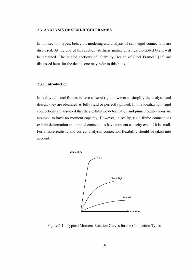
In reality, all steel frames behave as semi-rigid however to simplify the analysis and
design, they are idealized as fully rigid or perfectly pinned. In this idealization, rigid
connections are assumed that they exhibit no deformation and pinned connections are
assumed to have no moment capacity. However, in reality, rigid frame connections
exhibit deformation and pinned connections have moment capacity even if it is small.
For a more realistic and correct analysis, connection flexibility should be taken into
account.
Figure 2.1 - Typical Moment-Rotation Curves for the Connection Types
Rotation
Moment
Pinned
Semi-Rigid
Rigid
17
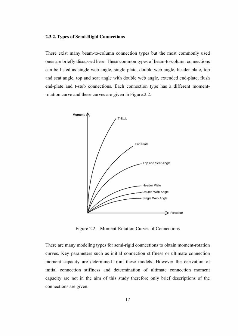
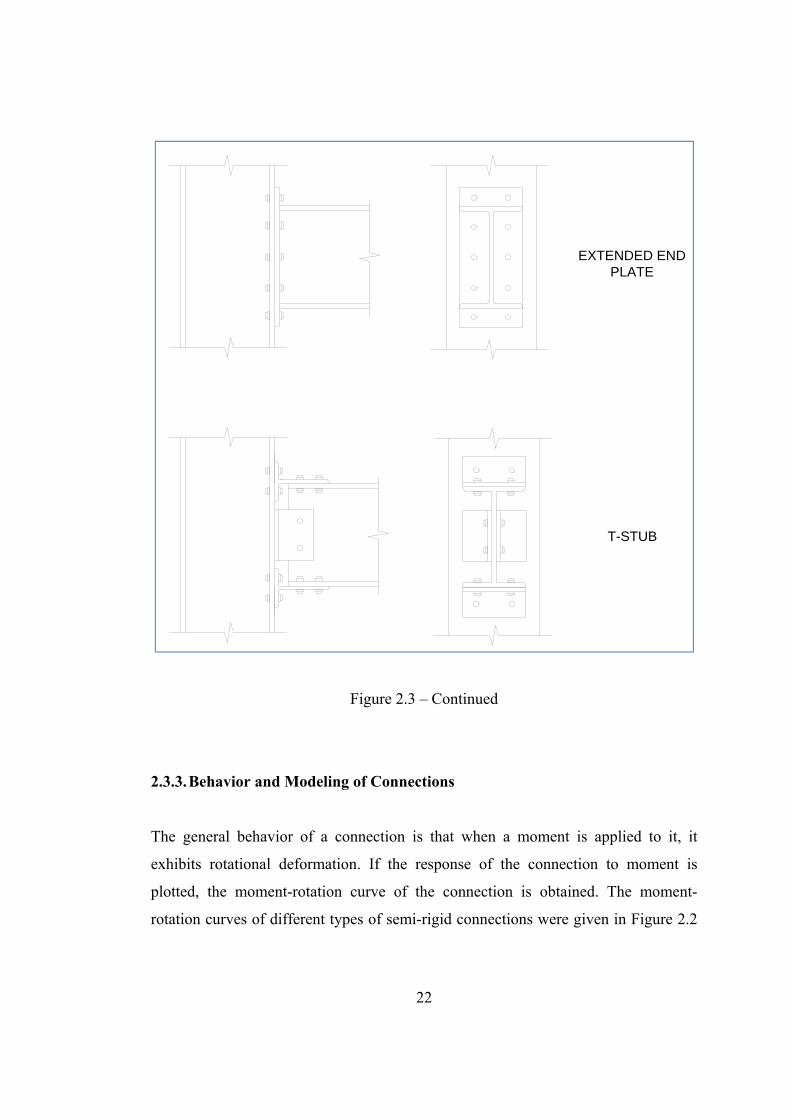
2.3.2. Types of Semi-Rigid Connections
There exist many beam-to-column connection types but the most commonly used
ones are briefly discussed here. These common types of beam-to-column connections
can be listed as single web angle, single plate, double web angle, header plate, top
and seat angle, top and seat angle with double web angle, extended end-plate, flush
end-plate and t-stub connections. Each connection type has a different moment-
rotation curve and these curves are given in Figure.2.2.
Figure 2.2 – Moment-Rotation Curves of Connections
There are many modeling types for semi-rigid connections to obtain moment-rotation
curves. Key parameters such as initial connection stiffness or ultimate connection
moment capacity are determined from these models. However the derivation of
initial connection stiffness and determination of ultimate connection moment
capacity are not in the aim of this study therefore only brief descriptions of the
connections are given.
Single Web Angle
Double Web Angle
Header Plate
Top and Seat Angle
End Plate
T-Stub
Rotation
Moment
18
Single Web Angle
The beam is connected to the column through an angle member, welded or bolted
both to the beam and column. This is a very flexible connection, it has very little
moment capacity and it is considered as shear connection.
Single Plate
In this connection, a plate is used instead of an angle member. The plate member is
welded or bolted to the beam and column. This connection type is also very flexible
and considered as shear connection.
Double Web Angle
The beam is connected to column through two angle members on the both side of the
beam web. The moment-rotation rigidity of this connection is higher than the
rigidities of single web angle and single plate connections however this connection
type is also considered as shear connection.
Header Plate Connections
Header plate connection consists of an end plate which is welded to the web of the
beam and bolted to the flange of the column. In this connection type, the length of
the plate is less than the depth of the beam. The moment-rotation rigidity of this
connection is similar to that of double web angle connection. This connection is also
considered as shear connection.
Top and Seat Angle Connections
This connection consists of two angle members welded or bolted to the beam, one is
at the bottom (seat angle) and the other one is at the top. The angles are bolted to the
column flange. The seat angle carries gravity loads but does not contribute
significantly to the moment capacity of the connection. The top angle is for the
lateral stability of the beam and does not carry any gravity loads. The experimental
results show that this type of connections is capable of resisting some of the end
moment of the beam.

19
Top and Seat Angle Connections with Double Web Angle
This connection is the combination of double web angle connection and top and seat
angle connection. This type is considered as semi-rigid connection.
Extended & Flush End-Plate Connections
Flush end-plate connections consist of a plate welded to the beam end (along both
top and bottom flanges and web) and bolted to the column. If the end-plate extends
on tension side or both on tension and compression sides, this connection type is
called extended end-plate connection. These two types of connections are considered
as moment connections.
T-stub Connections
This connection type is one of the stiffest connections and consists of two T-stubs
bolted to the beam at the top and bottom flange. The t-stubs are also bolted to the
column. This connection gets stiffer when used with double web angles.

20
Figure 2.3 – Types of Semi-Rigid Connections
SINGLE WEB ANGLE
SINGLE PLATE
DOUBLE WEB ANGLE
HEADER PLATE

21
Figure 2.3 – Continued
TOP AND SEATANGLE
TOP AND SEATANGLE WITHDOUBLE WEB
ANGLE
FLUSH END PLATE
22
Figure 2.3 – Continued
2.3.3. Behavior and Modeling of Connections
The general behavior of a connection is that when a moment is applied to it, it
exhibits rotational deformation. If the response of the connection to moment is
plotted, the moment-rotation curve of the connection is obtained. The moment-
rotation curves of different types of semi-rigid connections were given in Figure 2.2
EXTENDED ENDPLATE
T-STUB

23
and a typical moment-rotation behavior of a semi-rigid connection is given in Figure
2.4.
Figure 2.4 – Typical Moment-Rotation Behavior of a Semi-Rigid Connection
As it is seen in the Figure 2.4, the behavior of the connection is nonlinear. Factors
such as bolt slip, stress concentration and local yielding lead connection to exhibit
nonlinear response. Also the response of the connection to loading and unloading is
different. To predict the actual behavior of the connection, nonlinearity and
loading/unloading characteristic of the connection should be accounted for modeling
the connection. There are many types of models such as linear models (linear, bi-
linear, piecewise linear), polynomial model, b-spline model, power models and
exponential models. Among these models, linear model is the weakest model to
predict the actual behavior of the structure however it is the simplest one. Since the
aim of this study is to compare effective length method and direct analysis method in
semi-rigid frames and to investigate the effect of flexible connections to stability, it
is sufficient to use the linear connection model. The linear model is shown in Figure
2.4. The only parameter in linear model is the initial stiffness, Rki.
Rotation
Moment
1
Rki
1
Rki
unloading
loading
1Rkt
Rki = Initial Stiffness
Rkt = Tangent Stiffness
Linear
24
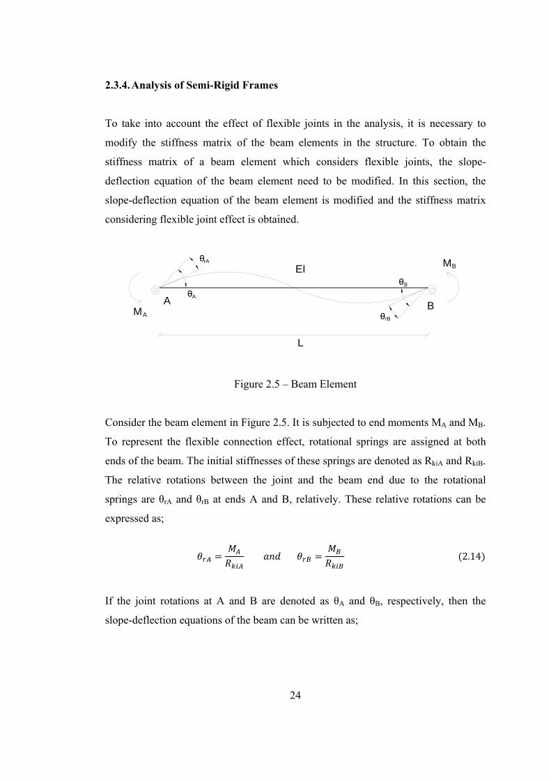
2.3.4. Analysis of Semi-Rigid Frames
To take into account the effect of flexible joints in the analysis, it is necessary to
modify the stiffness matrix of the beam elements in the structure. To obtain the
stiffness matrix of a beam element which considers flexible joints, the slope-
deflection equation of the beam element need to be modified. In this section, the
slope-deflection equation of the beam element is modified and the stiffness matrix
considering flexible joint effect is obtained.
Figure 2.5 – Beam Element
Consider the beam element in Figure 2.5. It is subjected to end moments MA and MB.
To represent the flexible connection effect, rotational springs are assigned at both
ends of the beam. The initial stiffnesses of these springs are denoted as RkiA and RkiB.
The relative rotations between the joint and the beam end due to the rotational
springs are θrA and θrB at ends A and B, relatively. These relative rotations can be
expressed as;
2.14
If the joint rotations at A and B are denoted as θA and θB, respectively, then the
slope-deflection equations of the beam can be written as;
A BMA
MBrA
A
B
rB
L
EI0
0
0
0

25
4 2 4 2 2.15
2 4 2 4 2.15
The equations 2.15a and 2.15b can be expressed as;
· · 2.16
· · 2.16
Where
412
2.17
412
2.17
2 2.17
In which
14
· 14
·4·
2.18

26
Figure 2.6 – Degrees of Freedom
For the degrees of freedom shown in the Figure 2.6, the stiffness matrix of the beam
is obtained as;
0 0 0 0
02
02
0 0
0 0 0 0
02
02
0 0
2.19
End-Fixity Factor
In the analysis of semi-rigid frames, EI/L represents the stiffness of the beam
member and Rki represents the stiffness of connection. There should be a relation
between these two such that it gives a physical interpretation of the rigidity available
in the connection [7].
Monforton and Wu [6] define an end-fixity factor and suggest a formula;
1
13 2.20
d1
d2
d3
d4
d5
d6

27
End-fixity factor, r, is an indicator of the relation between the beam stiffness and the
connection stiffness. It simplifies the analysis procedure and provides designers to
compare the structural responses of a member with semi-rigid connections [7]. The
upper and lower boundaries of end-fixity factor can be checked by setting connection
stiffness, Rki, to 1 N·m and 106 N·m;
1 · 1
13
1
130001
13001
0.00033 0.00
10 · 1
13
1
1300010
11.003
0.99701 1.00
As the connection stiffness approaches to zero which is the case of a pin connection,
the end-rigidity (r) approaches to zero and as the stiffness approaches to infinity
which is a fully rigid connection case, r approaches to 1.
The Eqn. 2.20 suggested by Monforton and Wu [6] is also used in this thesis. The
connection stiffnesses in the case studies are determined by this equation.
28
2.4. APPROXIMATE SECOND-ORDER ANALYSIS
In a structural analysis, if the original (or undeformed) geometry of the structure is
considered when writing the equilibrium and kinematic relationships then the
analysis is referred to as a first-order analysis. However, if the deformed geometry of
the structure is considered when writing the equilibrium and kinematic relationships
then the analysis is referred to as a second-order analysis. For the stability
consideration of structures, second-order analysis is a must [12]. Both of the stability
methods, Direct Analysis Method and Effective Length Method, require that a
rigorous second-order analysis including both P-∆ and P-δ effects. As an alternative
to a rigorous second-order analysis, the approximate method presented in Appendix
8 of the AISC 360-10 can be used. This method is based on the amplification of first-
order analysis forces and moments by the multipliers, B1 and B2. The B1 factor
accounts for P-δ effects and the B2 factor accounts for P-∆ effects. B1 is a member
parameter and applied to the moment due to gravity loads to account for the
displacements between the two ends of the column member. B2 is a story parameter
and applied to the moment and axial force due to the lateral loads to account for the
lateral displacement of the story.
The approximate second-order moment and axial force are determined as follows;
· · 2.21
· 2.22
Where
Mlt = 1st order moment due to lateral translation of the structure only (N·m)
Mnt = 1st order moment with the structure restrained against lateral translation
(N·m)
Mr = required 2nd order flexural strength (N·m)
Plt = 1st order axial force due to lateral translation of the structure only (N)

29
Pnt = 1st order axial force with the structure restrained against lateral
translation (N)
Pr = required 2nd order axial strength (N)
Calculation of B1
B1 is a member parameter and for each member it is calculated as follows;
11 2.23
Where
Cm = coefficient assuming no lateral translation of the frame determined
as follows:
a) For beam-columns not subjected to transverse loading between
supports in the plane of bending
0.6 0.4 · / 2.24
Where M1 and M2 are the smaller and larger moments,
respectively, at the ends of that portion of the member unbraced in
the plane of bending under consideration. M1/M2 is positive when
the member is bent in reverse curvature, negative when bent in
single curvature.
b) For beam-columns subject to transverse loading between supports,
the value of Cm shall be determined either by analysis or
conservatively taken as 1.0 for all cases.

30
Pe1 = elastic critical buckling strength of the member in the plane of
bending, calculated based on the assumption of no lateral translation
at the member ends (N)
· 2.25
EI* = flexural rigidity required to be used in the analysis (=0.8τbEI
when used in DAM)
K1 = effective length factor in the plane of bending, calculated
based on the assumption of no lateral translation at the
member ends, set equal to 1.0 unless analysis justifies a
smaller value
Calculation of B2
B2 is a story parameter and calculated for each story and each direction of lateral translation as follows;
1
1
1.0 2.26
Where
Pstory = total vertical load supported by the story including loads in
columns that are not part of the lateral force resisting system
(N)
Pestory = elastic critical buckling strength for the story in the direction
of translation being considered and calculated as;

31
∆ 2.27
Where
RM = 1 – 0.15·(Pmf/Pstory)
L = story height (mm)
Pmf = total vertical load in columns in the story that are part of
moment frames, if any, in the direction of translation being
considered (N)
ΔH = 1st order interstory dirft, in the direction of translation being
considered, due to lateral forces computed using the stiffness
required to be used in the analysis (mm).
H = story shear, in the direction of translation being considered,
produced by the lateral forces used to compute ΔH.

32
CHAPTER 3
CASE STUDIES
3.1. GENERAL INFORMATION AND ASSUMPTIONS
To compare DAM and ELM in semi-rigid frames, four case studies are analyzed. In
each case study, a frame is designed according to AISC 360-10 and stability design
of these frames is conducted according to both DAM and ELM. 21 analyses are
performed for different values of end-fixity factor (ranging from 0 to 1 with 0.05
increments) for each stability method. Total of 168 analyses are performed for the
four cases. The analyses are performed with Microsoft Office – Excel software
however for each case, one of the analyses is described in details for both ELM and
DAM in Sections 3.2, 3.3, 3.4 and 3.5 to explain the procedure in Excel spreadsheets.
For each case study and for each stability method, the analysis with end-fixity factor
of 0.75 is selected to be performed in this chapter. The analyses are summarized in
Figure 3.1.
Figure 3.1 – Summary of Analyses
ELM ELM
DAM DAM
ELM ELM
DAM DAM
r = 1.00 r = 1.00
21
Analyses: :
r = 0.95 r = 0.95
Case Study ‐ III Case Study ‐ IV
r = 0.00 r = 0.00r = 0.05 21
Analyses
r = 0.05
21
Analyses: :
r = 0.95r = 1.00 r = 1.00
r = 0.00 r = 0.00r = 0.05
21
Analyses
r = 0.05
r = 1.00
21
Analyses
21
Analyses
21
Analyses
21
Analyses
r = 0.95
Case Study ‐ II
r = 0.00r = 0.05
:r = 0.95
r = 0.95
:
r = 0.00
Case Study ‐ I
r = 0.00r = 0.05
:r = 0.95r = 1.00
r = 0.00
r = 1.00
r = 0.05
r = 1.00
r = 0.05:
r = 0.95

33
Each ELM analysis consists of structural analysis, buckling analysis and column
design parts whereas DAM consists of structural analysis and column design parts.
The flowcharts of both ELM and DAM are given in Figure 3.2.
Figure 3.2 – Flowcharts of ELM and DAM
EFFECTIVE LENGTH METHOD
INPUT PROCESS
COLUMN CAPACITY
AISC 360‐10
Column
Des ign
Equations
i ) Effective
length
FRAME
ANALYSIS RESULTS
FRAME
EFFECTIVE LENGTH
INPUT PROCESS
2nd Order
Structura l
Analys i s
i ) Loads
i i ) End‐fi xi ty
Buckl ing
Analys i si ) End‐fixi ty
FRAME COLUMN
(Pc , Mc)
(Pr , Mr)
COMBINED FORCES CHECK
DIRECT ANALYSIS METHOD
INPUT PROCESS INPUT PROCESS
(Pr , Mr) (Pc , Mc)
COMBINED FORCES CHECK
i ) Loads
i i ) End‐fi xi ty
2nd Order
Structura l
Analys i s
i ) End‐fixi ty
i i ) Effective
Length = 1.0
AISC 360‐10
Column
Des ign
Equations
ANALYSIS RESULTS COLUMN CAPACITY

34
The general overview of the case studies is given in Figure 3.3.
Case – I
Case – II
Case – III
Case – IV
Figure 3.3 – The General Overview of Case Studies
300 kN 300 kN
175 kN
HEA300
IPE500
HEA300
1000 kN 1000 kN
115 kN
HEA300
IPE500
HEA300
1900 kN 1900 kN
40 kN
HEA300
IPE500
HEA300
300 kN 550 kN 550 kN 300 kN
200 kN
HEA300 HEA300 HEA300 HEA300
IPE500IPE500 IPE500

35
Some general assumptions are made for the case studies. These can be listed as
below;
1. All column-to-base connections are fixed whereas all beam-to-column
connections are semi-rigid.
2. All springs (representing semi-rigid connections) in each case are identical, in
other words they have the same stiffnesses.
3. In all cases, columns are HEA300 and beams are IPE500.
4. All members are made of the same material and they have the same yield
strength, Fy = 345 MPa.
5. The beam members are assumed as axially rigid.
6. All columns, regardless of their orientation, are assumed as braced at their
midpoint in out-of-plane direction. In other words, out-of-plane length of the
columns is half of the in-plane length.
7. The applied loads are assumed as factored loads therefore no need to multiply
these loads with load factors again.
8. Load and Resistance Factor Design (LRFD) is adopted for design
calculations.
The physical properties of sections HEA300 and IPE500 are given in Table 3.1.

36
b
wh
t
ft
y
x
Table 3.1 – Physical Properties of Sections
HEA300 IPE500 E : elastic modulus 200000 MPa 200000 MPa Fy : yield strength 345 MPa 345 MPa b : width of the flange 300 mm 200 mm h : total depth 290 mm 500 mm tf : thickness of flange 14 mm 16 mm tw : thickness of web 8.5 mm 10.2 mm Ix : moment of inertia in x-dir. 182600000 mm4 482000000 mm4 Iy : moment of inertia in y-dir. 63100000 mm4 21420000 mm4 A : cross-sectional area 11300 mm2 11300 mm2 rx : radius of gyration in x-dir. 127.1 mm 203.8 mm ry : radius of gyration in y-dir. 74.7 mm 43.0 mm J : torsional constant 878000 mm4 891000 mm4 Sx : section modulus about x-axis 1259310 mm3 1928000 mm3 Sy : section modulus about y-axis 420667 mm3 214200 mm3 Zx : plastic section modulus about x-axis 1833000 mm3 2194000 mm3 Zy : plastic section modulus about y-axis 641000 mm3 336000 mm3
37
300 kN 300 kN
175 kNu
10
v1 v2
20
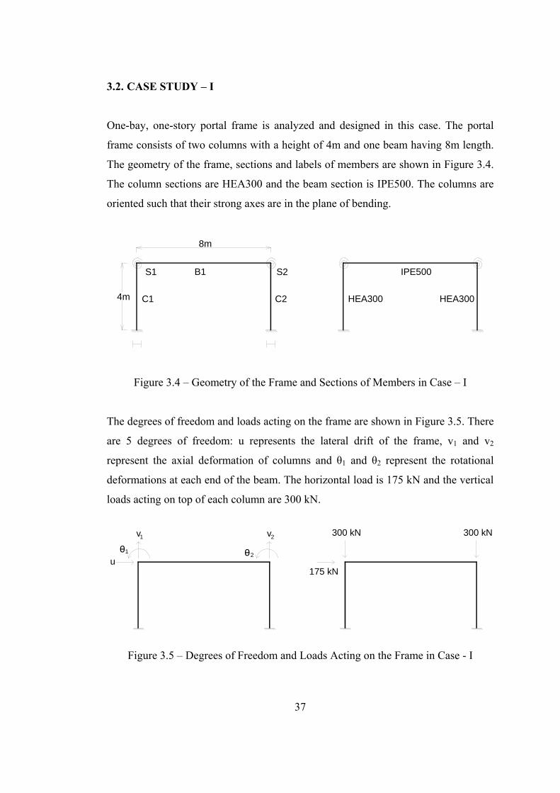
3.2. CASE STUDY – I
One-bay, one-story portal frame is analyzed and designed in this case. The portal
frame consists of two columns with a height of 4m and one beam having 8m length.
The geometry of the frame, sections and labels of members are shown in Figure 3.4.
The column sections are HEA300 and the beam section is IPE500. The columns are
oriented such that their strong axes are in the plane of bending.
Figure 3.4 – Geometry of the Frame and Sections of Members in Case – I
The degrees of freedom and loads acting on the frame are shown in Figure 3.5. There
are 5 degrees of freedom: u represents the lateral drift of the frame, v1 and v2
represent the axial deformation of columns and θ1 and θ2 represent the rotational
deformations at each end of the beam. The horizontal load is 175 kN and the vertical
loads acting on top of each column are 300 kN.
Figure 3.5 – Degrees of Freedom and Loads Acting on the Frame in Case - I
8m
4m C1 C2
B1S1 S2
HEA300
IPE500
HEA300

38
The portal frame is analyzed and designed with an end-fixity factor of 0.75 by using
both stability methods, DAM and ELM.
3.2.1. Design with Effective Length Method
To design columns in the frame, first-order structural analysis should be conducted,
and then the buckling length of the columns should be determined. At the end, the
columns are designed according to AISC 360-10 Chapter H1.
As explained in Section 2.2, nominal stiffnesses of members are used during design
with ELM. In addition, there is no need to use notional loads since there exists a
horizontal load and the drift ratio is smaller than 1.5 (calculated in Section 3.2.1.1 as
B2).
3.2.1.1. Structural Analysis
Structural analysis of the frame is conducted by using stiffness method. First, the
stiffness matrices of members are constructed then the system matrix is obtained. For
the beam, stiffness matrix in Eqn. 2.19 in Section 2.3.4 is used. For the columns, the
stiffness matrix in Eqn. 3.1 for the degrees of freedom given in Figure 3.6 is used.
Figure 3.6 – Degrees of Freedom for the Stiffness Matrix in Eqn. 3.1
d1
d2
d3
d4
d5
d6

39
0 0 0 0
012 6
012 6
06 4
06 2
0 0 0 0
012 6
012 6
06 2
06 4
3.1
Since the columns are identical, their stiffness matrices are identical too. For the
physical properties of HEA300 given in Table 3.1 (E, I and A) and column length of
4m (L), the stiffness matrix in Eqn. 3.1 becomes (units are in N and mm),
5.65 10 0 0 5.65 10 0 0
0 6.85 10 1.37 10 0 6.85 10 1.37 10
0 1.37 10 3.65 10 0 1.37 10 1.83 10
5.65 10 0 0 5.65 10 0 0
0 6.85 10 1.37 10 0 6.85 10 1.37 10
0 1.37 10 1.83 10 0 1.37 10 3.65 10
3.2
The displacement matrices of columns are,
000
000
3.3 & 3.3
40
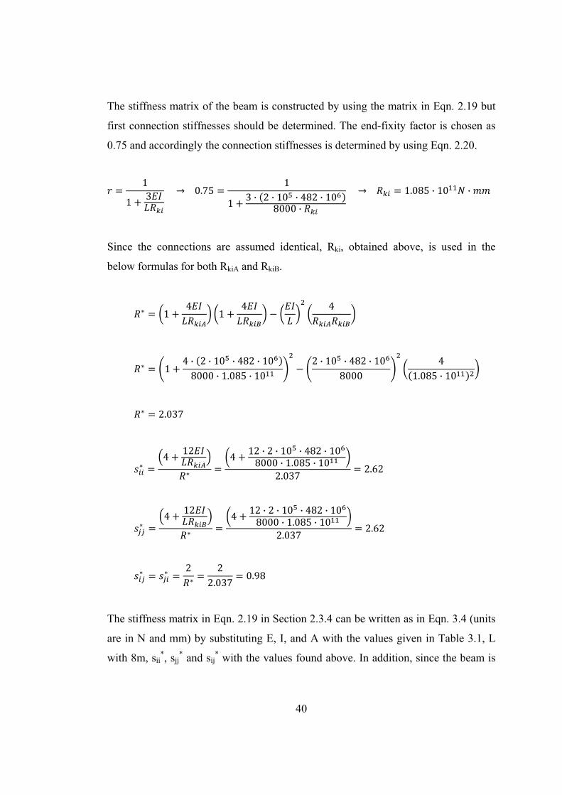
The stiffness matrix of the beam is constructed by using the matrix in Eqn. 2.19 but
first connection stiffnesses should be determined. The end-fixity factor is chosen as
0.75 and accordingly the connection stiffnesses is determined by using Eqn. 2.20.
1
13 0.75
1
13 · 2 · 10 · 482 · 10
8000 ·
1.085 · 10 ·
Since the connections are assumed identical, Rki, obtained above, is used in the
below formulas for both RkiA and RkiB.
14
14 4
14 · 2 · 10 · 482 · 108000 · 1.085 · 10
2 · 10 · 482 · 108000
41.085 · 10
2.037
412
412 · 2 · 10 · 482 · 108000 · 1.085 · 10
2.0372.62
412
412 · 2 · 10 · 482 · 108000 · 1.085 · 10
2.0372.62
2 22.037
0.98
The stiffness matrix in Eqn. 2.19 in Section 2.3.4 can be written as in Eqn. 3.4 (units
are in N and mm) by substituting E, I, and A with the values given in Table 3.1, L
with 8m, sii*, sjj
* and sij* with the values found above. In addition, since the beam is
41
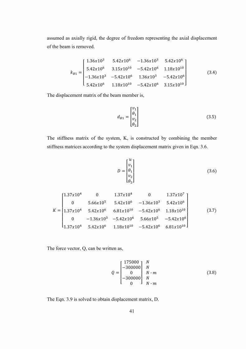
assumed as axially rigid, the degree of freedom representing the axial displacement
of the beam is removed.
1.36 10 5.42 10 1.36 10 5.42 10
5.42 10 3.15 10 5.42 10 1.18 10
1.36 10 5.42 10 1.36 10 5.42 10
5.42 10 1.18 10 5.42 10 3.15 10
3.4
The displacement matrix of the beam member is,
3.5
The stiffness matrix of the system, K, is constructed by combining the member
stiffness matrices according to the system displacement matrix given in Eqn. 3.6.
3.6
1.37 10 0 1.37 10 0 1.37 10
0 5.66 10 5.42 10 1.36 10 5.42 10
1.37 10 5.42 10 6.81 10 5.42 10 1.18 10
0 1.36 10 5.42 10 5.66 10 5.42 10
1.37 10 5.42 10 1.18 10 5.42 10 6.81 10
3.7
The force vector, Q, can be written as,
1750003000000
3000000
·
·
3.8
The Eqn. 3.9 is solved to obtain displacement matrix, D.

42
3.9
The inverse of system stiffness matrix is taken and K-1 is obtained.
1.11 10 3.65 10 1.91 10 3.65 10 1.91 10
3.65 10 1.77 10 1.83 10 7.38 10 1.83 10
1.91 10 1.83 10 1.85 10 1.83 10 6.69 10
3.65 10 7.38 10 1.83 10 1.77 10 1.83 10
1.91 10 1.83 10 6.69 10 1.83 10 1.85 10
3.10
Multiplying K-1 by Q gives the displacement matrix D.
1.11 10 3.65 10 1.91 10 3.65 10 1.91 10
3.65 10 1.77 10 1.83 10 7.38 10 1.83 10
1.91 10 1.83 10 1.85 10 1.83 10 6.69 10
3.65 10 7.38 10 1.83 10 1.77 10 1.83 10
1.91 10 1.83 10 6.69 10 1.83 10 1.85 10
175000
300000
0
300000
0
19.470
0.4671
0.0033
0.5949
0.0033
19.4700.46710.00330.59490.0033
3.11
After the displacement matrix D is determined, it is multiplied with member stiffness
matrices to obtain the member forces. For columns, C1 and C2, the stiffness matrix
in Eqn. 3.2 and displacement matrices in Eqn. 3.3a and Eqn. 3.3b are used,
respectively. For the beam, stiffness matrix in Eqn. 3.4 and displacement matrix in
Eqn. 3.5 are used.

43
Member forces for C1 is (units are in kN and m),
5.65 10 0 0 5.65 10 0 0
0 6.85 10 1.37 10 0 6.85 10 1.37 10
0 1.37 10 3.65 10 0 1.37 10 1.83 10
5.65 10 0 0 5.65 10 0 0
0 6.85 10 1.37 10 0 6.85 10 1.37 10
0 1.37 10 1.83 10 0 1.37 10 3.65 10
0.4671
19.470
0.0033
0
0
0
263.9
87.5
144.5
263.9
87.5
205.5
Member forces for C2 is (units are in kN and m),
5.65 10 0 0 5.65 10 0 0
0 6.85 10 1.37 10 0 6.85 10 1.37 10
0 1.37 10 3.65 10 0 1.37 10 1.83 10
5.65 10 0 0 5.65 10 0 0
0 6.85 10 1.37 10 0 6.85 10 1.37 10
0 1.37 10 1.83 10 0 1.37 10 3.65 10
0.5949
19.470
0.0033
0
0
0
336.1
87.5
144.5
336.1
87.5
205.5
Member forces for B1 is (units are in kN and m),
1.36 10 5.42 10 1.36 10 5.42 10
5.42 10 3.15 10 5.42 10 1.18 10
1.36 10 5.42 10 1.36 10 5.42 10
5.42 10 1.18 10 5.42 10 3.15 10
0.4671
0.0033
0.5949
0.0033
36.1
144.5
36.1
144.5
These are the first order analysis results and can be shown on the system as in Figure
3.7.

44
Figure 3.7 – First-Order Analysis Results of Case – I with ELM
As seen from the results, the critical column is C2 since the axial compressive force
is higher on C2. C2 governs the column design therefore the first-order forces and
moments of C2 are converted to second-order forces and moments with the
approximate method described in Section 2.4. The second order design axial load Pr
and design bending moment Mr are calculated as,
· · · 0 1.0200 · 205.5 209.7 ·
· 300 1.02 · 36.1 336.8 ·
0 ·
205.5 ·
-263.9 kN -336.1 kN
87.5 kN 87.5 kN
36.1 kN
205.5 kN.m
144.5 kN.m 144.5 kN.m
205.5 kN.m
SHEAR FORCE
MOMENT
AXIAL FORCE

45
300
336.1 300 36.1
1
1·
1
1 1 · 60030560
1.02
300 300 600
·∆
0.85 ·175 · 400019.47
30560
1 0.15 · 1 0.15 ·600600
0.85
∆ 19.47
As a summary, the second-order design forces and moments for the critical column
C2 are,
Pr = 336.8 kN Mr = 209.7 kN.m
3.2.1.2. Buckling Analysis
Buckling length of the frame is determined by setting the determinant of the stiffness
matrix of the system equal to zero. However, during constructing the stiffness matrix,
the column matrices shall be modified as described in Section 2.2 and so the stability
functions including the term K (effective length factor) are included into the system.
The smallest value of K, which makes the determinant equal to zero, is the buckling
length of the frame.
The buckling analyses are performed with the help of Microsoft Office – Excel and
in this section the calculation procedure in the spreadsheet is explained. The effective
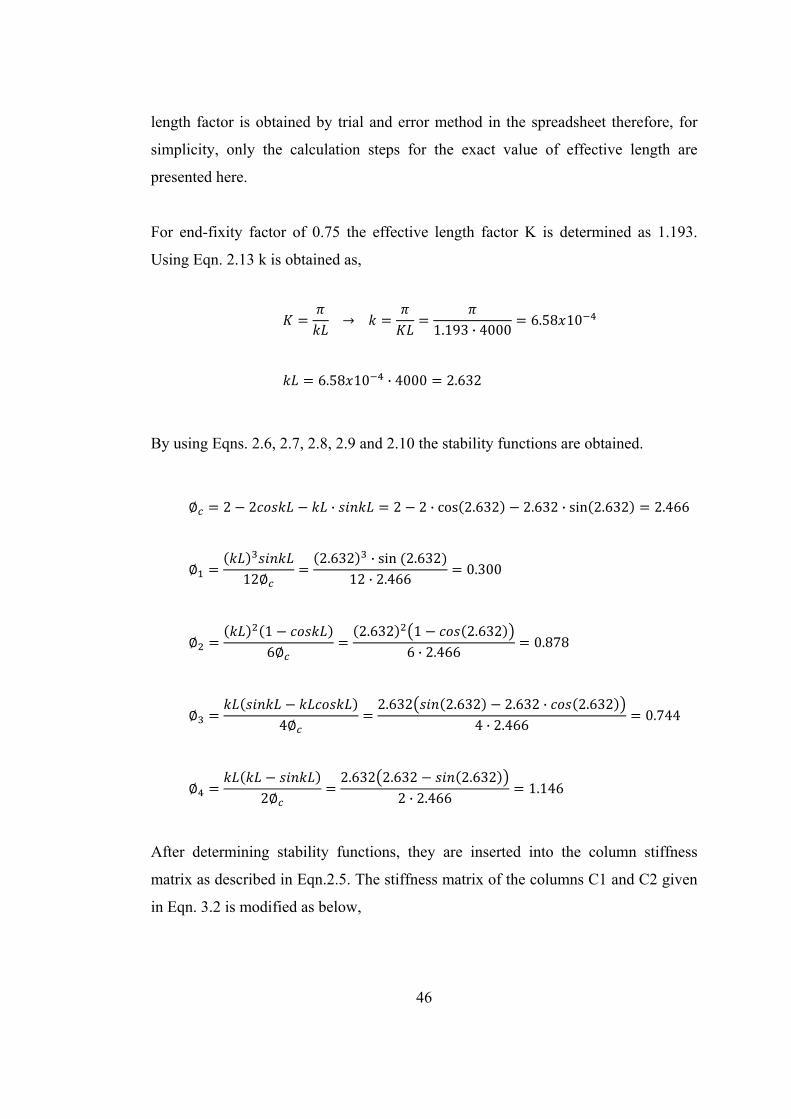
46
length factor is obtained by trial and error method in the spreadsheet therefore, for
simplicity, only the calculation steps for the exact value of effective length are
presented here.
For end-fixity factor of 0.75 the effective length factor K is determined as 1.193.
Using Eqn. 2.13 k is obtained as,
1.193 · 4000
6.58 10
6.58 10 · 4000 2.632
By using Eqns. 2.6, 2.7, 2.8, 2.9 and 2.10 the stability functions are obtained.
2 2 · 2 2 · cos 2.632 2.632 · sin 2.632 2.466
122.632 · sin 2.632
12 · 2.4660.300
16
2.632 1 2.6326 · 2.466
0.878
42.632 2.632 2.632 · 2.632
4 · 2.4660.744
22.632 2.632 2.632
2 · 2.4661.146
After determining stability functions, they are inserted into the column stiffness
matrix as described in Eqn.2.5. The stiffness matrix of the columns C1 and C2 given
in Eqn. 3.2 is modified as below,

47
5.65 10 0 0 5.65 10 0 0
0 2.06 10 1.20 10 0 2.06 10 1.20 10
0 1.20 10 2.72 10 0 1.20 10 2.09 10
5.65 10 0 0 5.65 10 0 0
0 2.06 10 1.20 10 0 2.06 10 1.20 10
0 1.20 10 2.09 10 0 1.20 10 2.72 10
System stiffness matrix is formed with combining column matrices calculated above
with the beam matrix obtained in Eqn. 3.4. In system stiffness matrix, elastic
modulus (E) is the same for all members and each term of the matrix includes E
therefore while taking the determinant of the matrix, E can be taken as a common
multiple. To simplify the calculation, the elastic modulus E is assumed as 1. The
system stiffness matrix with E=1 MPa is,
0.02 0 60.14 0 60.14
0 2.83 27.11 0.01 27.11
60.14 27.11 293625 27.11 59155
0 0.01 27.11 2.83 27.11
60.14 27.11 59155 27.11 293625
Determinant of K equals to zero.
3.2.1.3. Column Design
In this part, the axial compressive strength and moment capacity of a HEA300
column having 4m length and in-plane effective length factor of 1.193 are
determined and the column is checked under the combined effect of compression and
flexure.

48
In-plane flexural strength of the column is determined according to Chapter F of the
AISC 360-10. The in-plane flexural strength of C1 and C2 is Mc = 413.1 kN.m. The
calculation steps are given in Appendix A. The compressive strength of C1 and C2 is
Pc = 3164 kN. The calculation steps are given in Appendix B.
The check of the column considering the interaction of flexure and compression is
conducted according to Chapter H1 of AISC 360-10 and demand/capacity ratio is
obtained.
336.83164.0
0.106 0.200
⁄2
336.82 · 3164.0
209.7413.1
0.561 1.000
3.2.2. Design with Direct Analysis Method
In design according to DAM, the structural analysis is performed in the same way
with ELM however in DAM reduced stiffnesses are used instead of nominal
stiffnesses. The notional loads are not used in DAM too, with the same reason as in
ELM. The stiffness reduction factor is determined according to Section 2.1 (Eqn. 2.2
& 2.3). It requires an iterative procedure to determine the reduction factor. First, a τb
value is assumed and the structure is analyzed with this value then using the obtained
forces, the assumed τb value is checked whether it is acceptable or not. If it is
unacceptable, another value is assumed for τb and the same procedure is followed
until τb satisfies the conditions. For the Case – I, in the first iteration step, τb is
assumed as 1.0 and the structure is analyzed with the member stiffnesses reduced by
1.0x0.80 and the axial compressive load, Pr, is obtained as 337 kN (obtained in
Section 3.2.2.1) for the critical column C2.

49
1 · 33700011300 · 345
0.09 0.50 1.0
In the first iteration step τb is obtained. The stiffness reduction factor is 0.8 for both
columns, C1 and C2 and for the beam. The Pr value above is calculated for the
critical column C2, the axial load on C1 is smaller than the one on C2 therefore the
ratio for C1 is also smaller than 0.50.
3.2.2.1. Structural Analysis
The structural analysis by using DAM is conducted by using the same procedure as
described in ELM. Therefore, the calculation steps are skipped and only the resultant
stiffness matrix of the system, displacement matrix and member forces are presented.
The stiffness matrix of the system is,
1.10 10 0 1.10 10 0 1.10 10
0 4.53 10 4.34 10 1.08 10 4.34 10
1.10 10 4.34 10 5.45 10 4.34 10 9.46 10
0 1.08 10 4.34 10 4.53 10 4.34 10
1.10 10 4.34 10 9.46 10 4.34 10 5.45 10
The displacement matrix of the system is,
24.33800.58380.00420.74360.0042
The first-order analysis results are as in Figure 3.8.

50
Figure 3.8 – First-Order Analysis Result of Case – I with DAM
The second-order analysis results are obtained as;
· · · 0 1.0252 · 205.5 210.7 ·
· 300.0 1.0252 · 36.1 337.0 ·
0 ·
205.5 ·
300.0
-263.9 kN -336.1 kN
87.5 kN 87.5 kN
36.1 kN
205.5 kN.m
144.5 kN.m 144.5 kN.m
205.5 kN.m
SHEAR FORCE
MOMENT
AXIAL FORCE

51
336.1 300.0 36.1
1
1·
1
11 · 60024447
1.0252
300 300 600
·∆
0.85 ·175 · 400024.338
24447
1 0.15 · 1 0.15 ·600600
0.85
∆ 24.338
As a summary, the second-order design forces and moments for the critical column
C2 are,
Pr = 337.0 kN Mr = 210.7 kN.m
3.2.2.2. Column Design
In this part, the axial compressive strength and moment capacity of a HEA300
column with 4m length and in-plane effective length factor of 1.0 are determined and
the column is checked under the combined effect of compression and flexure.
In-plane flexural strength of the column is determined according to Chapter F of the
AISC 360-10. The in-plane flexural strength of C1 and C2 is Mc = 413.1 kN.m. The
calculation steps are given in Appendix A. The compressive strength of C1 and C2 is
Pc = 3263 kN. The calculation steps are given in Appendix B.
52
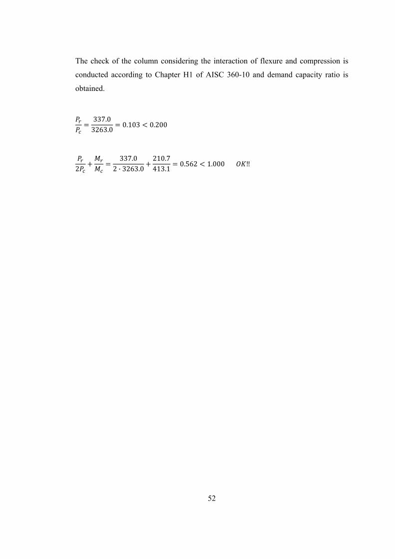
The check of the column considering the interaction of flexure and compression is
conducted according to Chapter H1 of AISC 360-10 and demand capacity ratio is
obtained.
337.03263.0
0.103 0.200
2337.0
2 · 3263.0210.7413.1
0.562 1.000

53
1000 kN 1000 kN
115 kNu
10
v1 v2
20
3.3. CASE STUDY – II
The portal frame in Case – I is analyzed and designed with different loads in this
case. The compressive loads are increased and the horizontal load is decreased. The
geometry of the frame, sections and labels of members are shown in Figure 3.9. The
degrees of freedom and loads acting on the frame are shown in Figure 3.10. The only
difference between this frame and the frame in Case – I is the loads acting on it.
Figure 3.9 – Geometry of the Frame and Sections of Members in Case – II
Figure 3.10 – Degrees of Freedom and Loads Acting on the Frame in Case - II
The portal frame is analyzed and designed with an end-fixity factor of 0.75 by using
both stability methods, DAM and ELM.
8m
4m C1 C2
B1S1 S2
HEA300
IPE500
HEA300

54
3.3.1. Design with Effective Length Method
In Case – II, like in Case – I, first structural analysis is conducted, then buckling
length of the columns is determined and at the end, the columns are designed. The
procedures used in Case – I to obtain member forces and buckling length of the
frame are followed in Case – II too, therefore in this part only the results are
presented, the steps are given in Appendix C. In analysis with ELM, nominal
stiffnesses of members are used and the notional loads are not used due to the
presence of a horizontal load.
3.3.1.1. Structural Analysis
The stiffness matrix of the system, displacement matrix, force vector and member
forces are presented here, for details of calculation please see Appendix C. The
stiffness matrix of the system is,
1.37 10 0 1.37 10 0 1.37 10
0 5.66 10 5.42 10 1.36 10 5.42 10
1.37 10 5.42 10 6.81 10 5.42 10 1.18 10
0 1.36 10 5.42 10 5.66 10 5.42 10
1.37 10 5.42 10 1.18 10 5.42 10 6.81 10
The displacement matrix D and force vector Q are,
12.7951.72790.00221.81190.0022
1150001000000
01000000
0
·
·
The first-order analysis results are as in Figure 3.11.

55
Figure 3.11 – First-Order Analysis Results of Case – II with ELM
The second-order design forces and moments for the critical column C2 are,
Pr = 1025.4 kN Mr = 144.5 kN.m
3.3.1.2. Buckling Analysis
The buckling analysis results for Case – II are the same with the results of Case – I
since the frames are identical. The loads on the frame do not affect the buckling
length of the frame. The buckling length of the frame for r = 0.75 is determined as
1.193.
-976.3 kN -1023.7 kN
57.5 kN 57.5 kN
23.7 kN
135.1 kN.m
94.9 kN.m 94.9 kN.m
135.1 kN.m
SHEAR FORCE
MOMENT
AXIAL FORCE

56
3.3.1.3. Column Design
In this part, the axial compressive strength and moment capacity of a HEA300
column having 4m length and in-plane effective length factor of 1.193 are
determined and the column is checked under the combined effect of compression and
flexure.
In-plane flexural strength of the column is determined according to Chapter F of the
AISC 360-10. The in-plane flexural strength of C1 and C2 is Mc = 413.1 kN.m. The
calculation steps are given in Appendix A. The compressive strength of C1 and C2 is
Pc = 3164 kN. The calculation steps are given in Appendix B.
The check of the column considering the interaction of flexure and compression is
conducted according to Chapter H1 of AISC 360-10 and demand/capacity ratio is
obtained.
1025.43164.0
0.324 0.200
⁄89·
1025.43164.0
89·144.5413.1
0.635 1.000
3.3.2. Design with Direct Analysis Method
The columns are designed with effective length factor of 1.0 after determining the
second-order forces from the structural analysis. During the analysis, reduced
stiffnesses are used and the notional loads are ignored due to the presence of a
horizontal load. The stiffness reduction factor is determined as described in Section
3.2.2. For the Case – II, the τb is obtained as 1.0 and the validity of it can be shown
as;
1 · 102580011300 · 345
0.26 0.50 1.0

57
3.3.2.1. Structural Analysis
The stiffness matrix of the system, displacement matrix, force vector and member
forces are presented here, for details of calculation please see Appendix C. The
stiffness matrix of the system is,
1.10 10 0 1.10 10 0 1.10 10
0 4.53 10 4.34 10 1.08 10 4.34 10
1.10 10 4.34 10 5.45 10 4.34 10 9.46 10
0 1.08 10 4.34 10 4.53 10 4.34 10
1.10 10 4.34 10 9.46 10 4.34 10 5.45 10
The displacement matrix D and force vector Q are,
15.9932.15990.00272.26490.0027
1150001000000
01000000
0
·
·
The first-order analysis results are as in Figure 3.12.
The second-order design forces and moments for the critical column C2 are,
Pr = 1025.8 kN Mr = 147.1 kN.m
3.3.2.2. Column Design
In this part, the axial compressive strength and moment capacity of a HEA300
column with 4m length and in-plane effective length factor of 1.0 are determined and
the column is checked under the combined effect of compression and flexure.

58
Figure 3.12 – First-Order Analysis Results of Case – II with DAM
In-plane flexural strength of the column is determined according to Chapter F of the
AISC 360-10. The in-plane flexural strength of C1 and C2 is Mc = 413.1 kN.m. The
calculation steps are given in Appendix A. The compressive strength of C1 and C2 is
Pc = 3263 kN. The calculation steps are given in Appendix B.
The check of the column considering the interaction of flexure and compression is
conducted according to Chapter H1 of AISC 360-10 and demand capacity ratio is
obtained.
1025.83263.0
0.314 0.200
⁄89·
1025.83263.0
89·147.1413.1
0.631 1.000
-976.3 kN -1023.7 kN
57.5 kN 57.5 kN
23.7 kN
135.1 kN.m
94.9 kN.m 94.9 kN.m
135.1 kN.m
SHEAR FORCE
MOMENT
AXIAL FORCE

59
1900 kN 1900 kN
40 kNu
10
v1 v2
20
3.4. CASE STUDY – III
The portal frame in Case – I and Case - II is analyzed and designed with different
loads in this case. The compressive loads are increased and the horizontal load is
decreased when compared with Case - II. The geometry of the frame, sections and
labels of members are shown in Figure 3.13. The degrees of freedom and loads
acting on the frame are shown in Figure 3.14. The only difference between this frame
and the frames in Case – I and Case - II is the loads acting on it.
Figure 3.13 – Geometry of the Frame and Sections of Members in Case – III
Figure 3.14 – Degrees of Freedom and Loads Acting on the Frame in Case - III
The portal frame is analyzed and designed with an end-fixity factor of 0.75 by using
both stability methods, DAM and ELM.
8m
4m C1 C2
B1S1 S2
HEA300
IPE500
HEA300
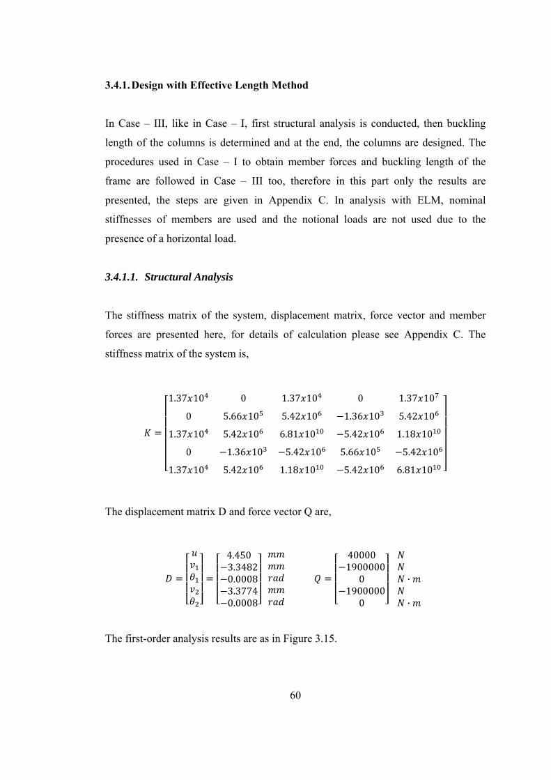
60
3.4.1. Design with Effective Length Method
In Case – III, like in Case – I, first structural analysis is conducted, then buckling
length of the columns is determined and at the end, the columns are designed. The
procedures used in Case – I to obtain member forces and buckling length of the
frame are followed in Case – III too, therefore in this part only the results are
presented, the steps are given in Appendix C. In analysis with ELM, nominal
stiffnesses of members are used and the notional loads are not used due to the
presence of a horizontal load.
3.4.1.1. Structural Analysis
The stiffness matrix of the system, displacement matrix, force vector and member
forces are presented here, for details of calculation please see Appendix C. The
stiffness matrix of the system is,
1.37 10 0 1.37 10 0 1.37 10
0 5.66 10 5.42 10 1.36 10 5.42 10
1.37 10 5.42 10 6.81 10 5.42 10 1.18 10
0 1.36 10 5.42 10 5.66 10 5.42 10
1.37 10 5.42 10 1.18 10 5.42 10 6.81 10
The displacement matrix D and force vector Q are,
4.4503.34820.00083.37740.0008
400001900000
01900000
0
·
·
The first-order analysis results are as in Figure 3.15.
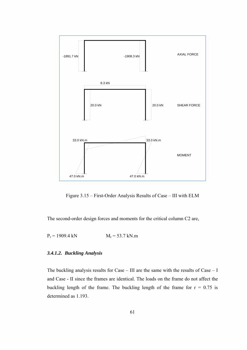
61
Figure 3.15 – First-Order Analysis Results of Case – III with ELM
The second-order design forces and moments for the critical column C2 are,
Pr = 1909.4 kN Mr = 53.7 kN.m
3.4.1.2. Buckling Analysis
The buckling analysis results for Case – III are the same with the results of Case – I
and Case - II since the frames are identical. The loads on the frame do not affect the
buckling length of the frame. The buckling length of the frame for r = 0.75 is
determined as 1.193.
-1891.7 kN -1908.3 kN
20.0 kN 20.0 kN
8.3 kN
47.0 kN.m
33.0 kN.m 33.0 kN.m
47.0 kN.m
SHEAR FORCE
MOMENT
AXIAL FORCE

62
3.4.1.3. Column Design
In this part, the axial compressive strength and moment capacity of a HEA300
column having 4m length and in-plane effective length factor of 1.193 are
determined and the column is checked under the combined effect of compression and
flexure.
In-plane flexural strength of the column is determined according to Chapter F of the
AISC 360-10. The in-plane flexural strength of C1 and C2 is Mc = 413.1 kN.m. The
calculation steps are given in Appendix A. The compressive strength of C1 and C2 is
Pc = 3164 kN. The calculation steps are given in Appendix B.
The check of the column considering the interaction of flexure and compression is
conducted according to Chapter H1 of AISC 360-10 and demand/capacity ratio is
obtained.
1909.43164.0
0.603 0.200
⁄89·
1909.43164.0
89·53.7413.1
0.719 1.000
3.4.2. Design with Direct Analysis Method
The columns are designed with effective length factor of 1.0 after determining the
second-order forces from the structural analysis. During the analysis, reduced
stiffnesses are used and the notional loads are ignored due to the presence of a
horizontal load. The stiffness reduction factor is determined as described in Section
3.2.2. For the Case – III, the τb is obtained as 1.0 and the validity of it can be shown
as;
1 · 190980011300 · 345
0.49 0.50 1.0
63
3.4.2.1. Structural Analysis
The stiffness matrix of the system, displacement matrix, force vector and member
forces are presented here, for details of calculation please see Appendix C. The
stiffness matrix of the system is,
1.10 10 0 1.10 10 0 1.10 10
0 4.53 10 4.34 10 1.08 10 4.34 10
1.10 10 4.34 10 5.45 10 4.34 10 9.46 10
0 1.08 10 4.34 10 4.53 10 4.34 10
1.10 10 4.34 10 9.46 10 4.34 10 5.45 10
The displacement matrix D and force vector Q are,
5.5634.18530.00104.22180.0010
400001900000
01900000
0
·
·
The first-order analysis results are as in Figure 3.16.
The second-order design forces and moments for the critical column C2 are,
Pr = 1909.8 kN Mr = 55.6 kN.m
3.4.2.2. Column Design
In this part, the axial compressive strength and moment capacity of a HEA300
column with 4m length and in-plane effective length factor of 1.0 are determined and
the column is checked under the combined effect of compression and flexure.
64
Figure 3.16 – First-Order Analysis Results of Case – III with DAM
In-plane flexural strength of the column is determined according to Chapter F of the
AISC 360-10. The in-plane flexural strength of C1 and C2 is Mc = 413.1 kN.m. The
calculation steps are given in Appendix A. The compressive strength of C1 and C2 is
Pc = 3263 kN. The calculation steps are given in Appendix B.
The check of the column considering the interaction of flexure and compression is
conducted according to Chapter H1 of AISC 360-10 and demand capacity ratio is
obtained.
1909.83263.0
0.585 0.200
⁄89·
1909.83263.0
89·55.6413.1
0.705 1.000
-1891.7 kN -1908.8 kN
20.0 kN 20.0 kN
8.3 kN
47.0 kN.m
33.0 kN.m 33.0 kN.m
47.0 kN.m
SHEAR FORCE
MOMENT
AXIAL FORCE
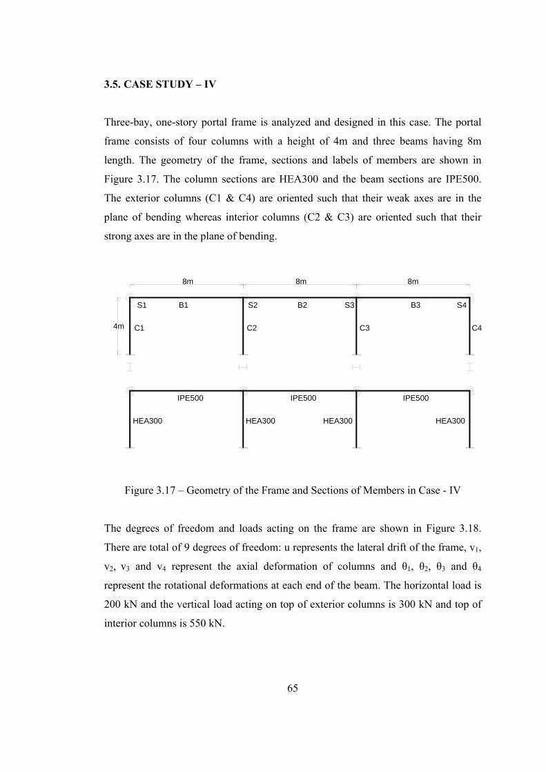
65
3.5. CASE STUDY – IV
Three-bay, one-story portal frame is analyzed and designed in this case. The portal
frame consists of four columns with a height of 4m and three beams having 8m
length. The geometry of the frame, sections and labels of members are shown in
Figure 3.17. The column sections are HEA300 and the beam sections are IPE500.
The exterior columns (C1 & C4) are oriented such that their weak axes are in the
plane of bending whereas interior columns (C2 & C3) are oriented such that their
strong axes are in the plane of bending.
Figure 3.17 – Geometry of the Frame and Sections of Members in Case - IV
The degrees of freedom and loads acting on the frame are shown in Figure 3.18.
There are total of 9 degrees of freedom: u represents the lateral drift of the frame, v1,
v2, v3 and v4 represent the axial deformation of columns and θ1, θ2, θ3 and θ4
represent the rotational deformations at each end of the beam. The horizontal load is
200 kN and the vertical load acting on top of exterior columns is 300 kN and top of
interior columns is 550 kN.
8m
4m
8m 8m
C1 C2 C3 C4
B1 B2 B3S1 S2 S3 S4
HEA300
IPE500
HEA300
IPE500
HEA300
IPE500
HEA300
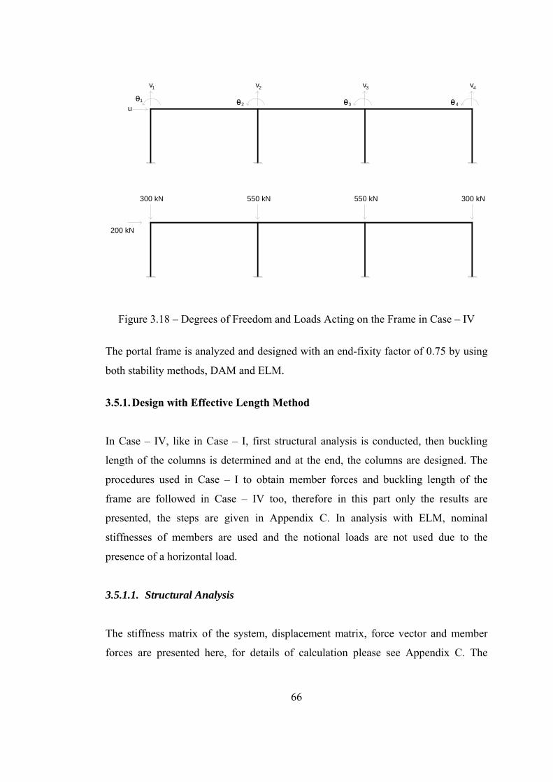
66
Figure 3.18 – Degrees of Freedom and Loads Acting on the Frame in Case – IV
The portal frame is analyzed and designed with an end-fixity factor of 0.75 by using
both stability methods, DAM and ELM.
3.5.1. Design with Effective Length Method
In Case – IV, like in Case – I, first structural analysis is conducted, then buckling
length of the columns is determined and at the end, the columns are designed. The
procedures used in Case – I to obtain member forces and buckling length of the
frame are followed in Case – IV too, therefore in this part only the results are
presented, the steps are given in Appendix C. In analysis with ELM, nominal
stiffnesses of members are used and the notional loads are not used due to the
presence of a horizontal load.
3.5.1.1. Structural Analysis
The stiffness matrix of the system, displacement matrix, force vector and member
forces are presented here, for details of calculation please see Appendix C. The
u1
2 3 40 0 0 0
300 kN 550 kN 550 kN 300 kN
200 kN
v1 v2 v3 v4

67
stiffness matrix of the system is given in Figure 3.20. The displacement matrix D and
force vector Q are,
13.7390.00110.00160.00160.00100.50620.96800.97810.5566
2000000300550550300
The first order analysis results are as in Figure 3.19.
Figure 3.19 – First-Order Analysis Results of Case – IV with ELM
-286.0 kN -546.9 kN -552.6 kN -314.5 kN
AXIAL FORCE
27.3kN 72.2 kN 72.8 kN 27.8 kN
SHEAR FORCE
14.0 kN17.1 kN
14.5 kN
58.1 kN.m
MOMENT
51.1 kN.m
159.0 kN.m 159.7 kN.m 58.7 kN.m
61.0 kN.m
68.8 kN.m
129.8 kN.m 131.3 kN.m
63.3 kN.m
68.0 kN.m
51.1 kN.m
52.4 kN.m
52.4 kN.m

68
1.84310
44.73310
61.37010
71.37010
74.73310
60
00
0
4.73310
64.41710
101.18310
100
05.42310
65.42310
60
0
1.37010
71.18310
109.96210
101.18310
100
5.42310
60
5.42310
60
1.37010
70
1.18310
109.96210
101.18310
100
5.42310
60
5.42310
6
4.73310
60
01.18310
104.41710
100
05.42310
65.42310
6
05.42310
65.42310
60
05.66410
51.35610
30
0
05.42310
60
5.42310
60
1.35610
35.67710
51.35610
30
00
5.42310
60
5.42310
60
1.35610
35.67710
51.35610
3
00
05.42310
65.42310
60
01.35610
35.66410
5
Figure 3.20 – The Stiffness Matrix of the System in Case – IV with ELM

69
The second-order design forces and moments for the critical columns are;
Critical interior column : C3 Pr = 552.7 kN Mr = 165.4 kN·m
Critical exterior column : C4 Pr = 315.0 kN Mr = 60.8 kN·m
3.5.1.2. Buckling Analysis
The buckling analysis is performed with Microsoft Office - Excel and the buckling
length of the frame is determined as 1.095. The resultant stiffness matrix of the
system is presented in Figure 3.21. Like in the Case – I, elastic modulus E is assumed
as 1 instead of 200000 to simplify the solution. The determinant of the matrix is
equal to zero.
3.5.1.3. Column Design
3.5.1.3.1. Design of Interior Columns
The compressive and flexural strength of interior columns (C2 & C3) are determined
and they are checked under the combined effect of compression and flexure. The in-
plane effective length factor is calculated as 1.095. In-plane flexural strength of the
column is determined according to Chapter F of the AISC 360-10. The in-plane
flexural strength of C2 and C3 is Mc = 413.1 kN.m. The calculation steps are given in
Appendix A. The compressive strength of C2 and C3 is Pc = 3216 kN. The
calculation steps are given in Appendix B. The check of the column considering the
interaction of flexure and compression is conducted according to Chapter H1 of
AISC 360-10 and demand capacity ratio is obtained.
552.73216.3
0.172 0.200
⁄2
552.72 · 3216.3
165.4413.1
0.486 1.000
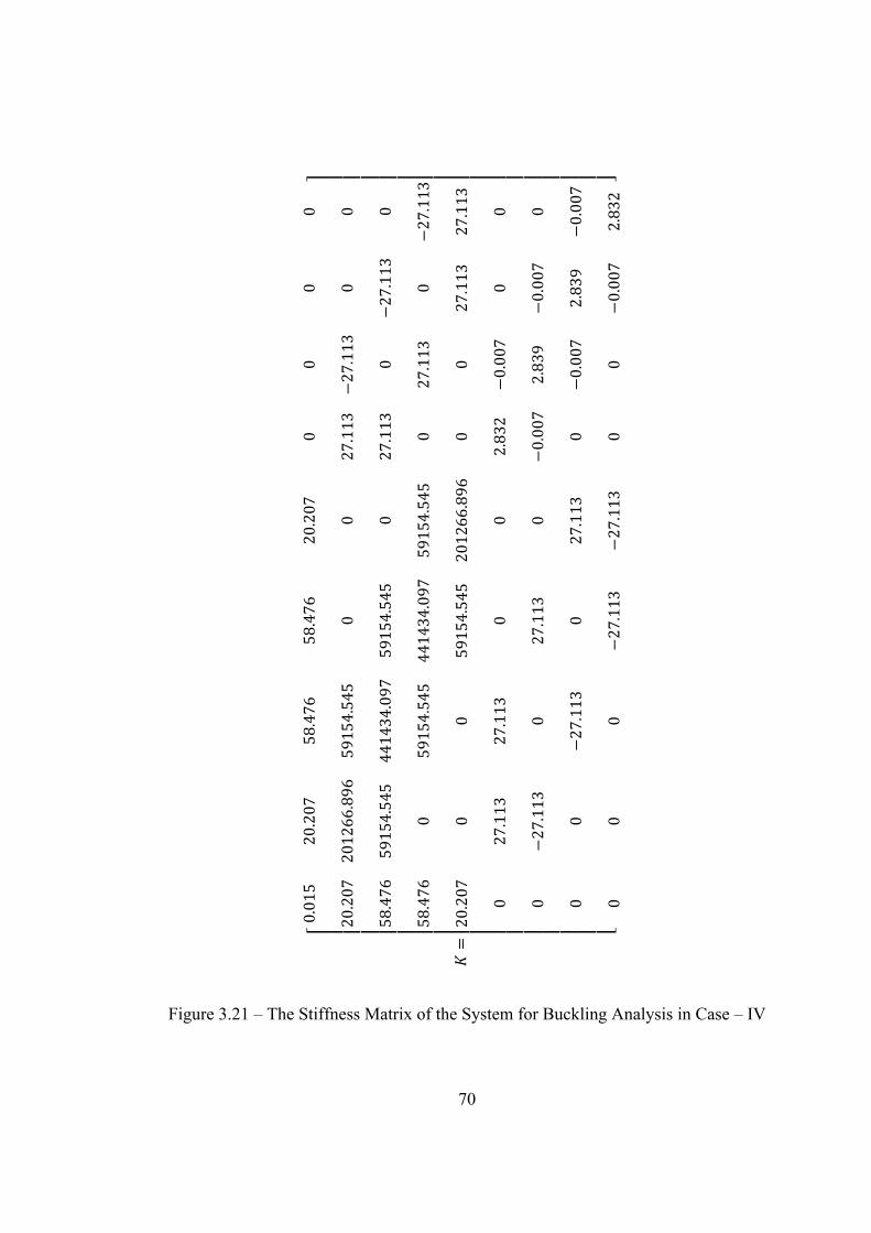
70
0.015
20.207
58.476
58.476
20.207
00
00
20.207
201266.896
59154.545
00
27.113
27.113
00
58.476
59154.545
441434.097
59154.545
027.113
027.113
0
58.476
059154.545
441434.097
59154.545
027.113
027.113
20.207
00
59154.545
201266.896
00
27.113
27.113
027.113
27.113
00
2.832
0.007
00
027.113
027.113
00.007
2.839
0.007
0
00
27.113
027.113
00.007
2.839
0.007
00
027.113
27.113
00
0.007
2.832
Figure 3.21 – The Stiffness Matrix of the System for Buckling Analysis in Case – IV

71
3.5.1.3.2. Design of Exterior Columns
The compressive and flexural strength of exterior columns (C1 & C4) are determined
and they are checked under the combined effect of compression and flexure. The in-
plane effective length factor is calculated as 1.095. In-plane flexural strength of the
column is determined according to Chapter F of the AISC 360-10. The in-plane
flexural strength of C1 and C4 is Mc = 187.8 kN.m. The calculation steps are given in
Appendix A. The compressive strength of C1 and C4 is Pc = 2732 kN. The
calculation steps are given in Appendix B. The check of the column considering the
interaction of flexure and compression is conducted according to Chapter H1 of
AISC 360-10 and demand capacity ratio is obtained.
315.02732.1
0.115 0.200
⁄2
315.02 · 2732.1
60.8187.8
0.381 1.000
3.5.2. Design with Direct Analysis Method
The columns are designed with effective length factor of 1.0 after determining the
second-order forces from the structural analysis. During the analysis, reduced
stiffnesses are used and the notional loads are ignored due to the presence of a
horizontal load. The stiffness reduction factor is determined as described in Section
3.2.2. For the Case – IV, the τb is obtained as 1.0 and the validity of it can be shown
as;
1 · 55280011300 · 345
0.14 0.50 1.0

72
3.5.2.1. Structural Analysis
The stiffness matrix of the system, displacement matrix, force vector and member
forces are presented here, for details of calculation please see Appendix C. The
stiffness matrix of the system is given in Figure 3.23. The displacement matrix D,
force vector Q and first-order analysis results are as below;
17.17410.00140.00200.00190.00130.63271.21001.22270.6957
2000000300550550300
Figure 3.22 – First-Order Analysis Results of Case – IV with DAM
-286.0 kN -546.9 kN -552.6 kN -314.5 kN
AXIAL FORCE
27.3kN 72.2 kN 72.8 kN 27.8 kN
SHEAR FORCE
14.0 kN17.1 kN
14.5 kN
58.1 kN.m
MOMENT
51.1 kN.m
159.0 kN.m 159.7 kN.m 58.7 kN.m
61.0 kN.m
68.8 kN.m
129.8 kN.m 131.3 kN.m
63.3 kN.m
68.0 kN.m
51.1 kN.m
52.4 kN.m
52.4 kN.m

73
1.47410
43.78610
61.09610
71.09610
73.78610
60
00
0
3.78610
63.53410
109.46510
90
04.33810
64.33810
60
0
1.09610
79.46510
97.96910
109.46510
90
4.33810
60
4.33810
60
1.09610
70
9.46510
97.96910
109.46510
90
4.33810
60
4.33810
6
3.78610
60
09.46510
93.53410
100
04.33810
64.33810
6
04.33810
64.33810
60
04.53110
51.08510
30
0
04.33810
60
4.33810
60
1.08510
34.54210
51.08510
30
00
4.33810
60
4.33810
60
1.08510
34.54210
51.08510
3
00
04.33810
64.33810
60
01.08510
34.53110
5
Figure 3.23 – The Stiffness Matrix of the System in Case – IV with DAM

74
The second-order design forces and moments for the critical columns are;
Critical interior column : C3 Pr = 552.8 kN Mr = 166.9 kN·m
Critical exterior column : C4 Pr = 315.1 kN Mr = 61.3 kN·m
3.5.2.2. Column Design
3.5.2.2.1. Design of Interior Columns
The compressive and flexural strength of interior columns (C2 & C3) are determined
and they are checked under the combined effect of compression and flexure. The in-
plane effective length factor is 1.00. In-plane flexural strength of the column is
determined according to Chapter F of the AISC 360-10. The in-plane flexural
strength of C2 and C3 is Mc = 413.1 kN.m. The calculation steps are given in
Appendix A. The compressive strength of C2 and C3 is Pc = 3263 kN. The
calculation steps are given in Appendix B. The check of the column considering the
interaction of flexure and compression is conducted according to Chapter H1 of
AISC 360-10 and demand capacity ratio is obtained.
552.83263.1
0.169 0.200
⁄2
552.82 · 3263.1
166.9413.1
0.489 1.000
3.5.2.2.2. Design of Exterior Columns
The compressive and flexural strength of exterior columns (C1 & C4) are determined
and they are checked under the combined effect of compression and flexure. The in-
plane effective length factor is calculated as 1.00. In-plane flexural strength of the
column is determined according to Chapter F of the AISC 360-10. The in-plane
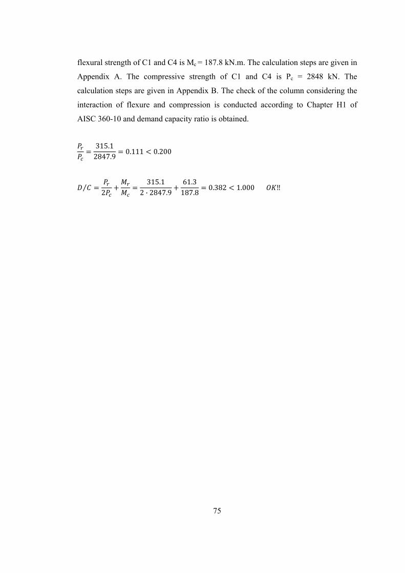
75
flexural strength of C1 and C4 is Mc = 187.8 kN.m. The calculation steps are given in
Appendix A. The compressive strength of C1 and C4 is Pc = 2848 kN. The
calculation steps are given in Appendix B. The check of the column considering the
interaction of flexure and compression is conducted according to Chapter H1 of
AISC 360-10 and demand capacity ratio is obtained.
315.12847.9
0.111 0.200
⁄2
315.12 · 2847.9
61.3187.8
0.382 1.000

76
CHAPTER 4
RESULTS AND DISCUSSIONS OF RESULTS
4.1. RESULTS
In Section 3.1, it is explained that there are total of 168 analyses. In Sections 3.2, 3.3,
3.4 and 3.5, for each case one analysis is explained in details and the results of that
analysis are presented at the end of those sections. In this section, all results for all
analyses are presented.
The terms used in the tables are explained as below;
r : end-rigidity factor
Pr : second-order design compressive load (kN)
Mr : second-order design moment (kN·m)
Pc : compressive strength (kN)
Mc : flexural strength (kN·m)
K : effective length factor
B2 : the ratio of second-order drift to first-order drift
D/C : demand/capacity ratio
In the tables given below, second-order forces and moments (Pr & Mr), member
compressive and flexural strengths (Pc & Mc), effective length factors (K), drift ratios
(B2) and demand/capacity ratios for all end-rigidity factors (ranging from 0 to 1) and
for both stability methods are presented. After each table, a figure showing the D/C
ratios for both stability methods is presented.

77
4.1.1. Results of Case - I
Analysis and design results of the critical column C2 in Case – I are presented in
Table 4.1.
Table 4.1 – Analysis and Design Results of C2 in Case – I
The demand/capacity ratios of C2 for ELM and DAM are drawn in Figure 4.1.
C1 C2
r Pr Mr Pc Mc K B2 D/C Pr Mr Pc Mc K B2 D/C
1.00 339.5 198.2 3203.4 413.1 1.120 1.018 0.533 339.7 199.1 3263.1 413.1 1.00 1.022 0.534
0.95 339.0 200.1 3196.6 413.1 1.133 1.018 0.537 339.2 201.0 3263.1 413.1 1.00 1.023 0.539
0.90 338.6 202.2 3189.7 413.1 1.146 1.018 0.543 338.7 203.1 3263.1 413.1 1.00 1.023 0.544
0.85 338.0 204.5 3182.2 413.1 1.160 1.019 0.548 338.2 205.4 3263.1 413.1 1.00 1.024 0.549
0.80 337.5 206.9 3174.2 413.1 1.175 1.019 0.554 337.6 208.0 3263.1 413.1 1.00 1.024 0.555
0.75 336.8 209.7 3164.9 413.1 1.192 1.020 0.561 337.0 210.7 3263.1 413.1 1.00 1.025 0.562
0.70 336.1 212.7 3154.4 413.1 1.211 1.021 0.568 336.3 213.8 3263.1 413.1 1.00 1.026 0.569
0.65 335.4 216.0 3143.3 413.1 1.231 1.021 0.576 335.6 217.2 3263.1 413.1 1.00 1.027 0.577
0.60 334.5 219.7 3130.3 413.1 1.254 1.022 0.585 334.7 220.9 3263.1 413.1 1.00 1.028 0.586
0.55 333.6 223.9 3115.9 413.1 1.279 1.023 0.595 333.7 225.2 3263.1 413.1 1.00 1.029 0.596
0.50 332.5 228.6 3099.6 413.1 1.307 1.024 0.607 332.7 229.9 3263.1 413.1 1.00 1.030 0.608
0.45 331.2 233.9 3080.6 413.1 1.339 1.025 0.620 331.4 235.4 3263.1 413.1 1.00 1.032 0.621
0.40 329.8 240.0 3058.8 413.1 1.375 1.027 0.635 330.0 241.6 3263.1 413.1 1.00 1.033 0.635
0.35 328.2 247.1 3033.5 413.1 1.416 1.028 0.652 328.4 248.9 3263.1 413.1 1.00 1.035 0.653
0.30 326.2 255.5 3003.9 413.1 1.463 1.030 0.673 326.4 257.4 3263.1 413.1 1.00 1.038 0.673
0.25 324.0 265.4 2969.0 413.1 1.517 1.032 0.697 324.1 267.5 3263.1 413.1 1.00 1.040 0.697
0.20 321.2 277.4 2926.6 413.1 1.581 1.035 0.726 321.4 279.8 3263.1 413.1 1.00 1.044 0.727
0.15 317.7 292.2 2875.5 413.1 1.656 1.038 0.763 317.9 295.0 3263.1 413.1 1.00 1.048 0.763
0.10 313.4 311.0 2811.6 413.1 1.747 1.042 0.809 313.5 314.3 3263.1 413.1 1.00 1.053 0.809
0.05 307.7 335.6 2730.4 413.1 1.859 1.047 0.869 307.8 339.6 3263.1 413.1 1.00 1.060 0.869
0.00 300.0 369.0 2624.7 413.1 2.000 1.054 0.950 300.0 374.1 3263.1 413.1 1.00 1.069 0.952
Effective Length Method Direct Analysis Method

78
0.500
0.550
0.600
0.650
0.700
0.750
0.800
0.850
0.900
0.950
1.000
0.00
0.05
0.10
0.15
0.20
0.25
0.30
0.35
0.40
0.45
0.50
0.55
0.60
0.65
0.70
0.75
0.80
0.85
0.90
0.95
1.00
D/C Ratio
End Rigidity
ELM
DAM
Figure 4.1 – Demand/Capacity vs. End-Rigidity for Case – I

79
4.1.2. Results of Case - II
Analysis and design results of the critical column C2 in Case – II are presented in
Table 4.2.
Table 4.2 – Analysis and Design Results of C2 in Case – II
The demand/capacity ratios of C2 for ELM and DAM are drawn in Figure 4.2.
C1 C2
r Pr Mr Pc Mc K B2 D/C Pr Mr Pc Mc K B2 D/C
1.00 1027.1 135.8 3203.4 413.1 1.120 1.061 0.613 1027.5 137.9 3263.1 413.1 1.00 1.077 0.612
0.95 1026.8 137.2 3196.6 413.1 1.133 1.063 0.617 1027.2 139.4 3263.1 413.1 1.00 1.079 0.615
0.90 1026.5 138.8 3189.7 413.1 1.146 1.064 0.621 1026.9 141.1 3263.1 413.1 1.00 1.081 0.618
0.85 1026.2 140.6 3182.2 413.1 1.160 1.066 0.625 1026.6 142.9 3263.1 413.1 1.00 1.084 0.622
0.80 1025.8 142.5 3174.2 413.1 1.175 1.068 0.630 1026.2 144.9 3263.1 413.1 1.00 1.086 0.626
0.75 1025.4 144.5 3164.9 413.1 1.192 1.070 0.635 1025.8 147.1 3263.1 413.1 1.00 1.089 0.631
0.70 1025.0 146.8 3154.4 413.1 1.211 1.072 0.641 1025.4 149.5 3263.1 413.1 1.00 1.092 0.636
0.65 1024.5 149.4 3143.3 413.1 1.231 1.075 0.647 1024.9 152.3 3263.1 413.1 1.00 1.096 0.642
0.60 1023.9 152.3 3130.3 413.1 1.254 1.078 0.655 1024.4 155.3 3263.1 413.1 1.00 1.099 0.648
0.55 1023.3 155.5 3115.9 413.1 1.279 1.081 0.663 1023.8 158.7 3263.1 413.1 1.00 1.104 0.655
0.50 1022.6 159.1 3099.6 413.1 1.307 1.085 0.672 1023.1 162.6 3263.1 413.1 1.00 1.109 0.663
0.45 1021.8 163.3 3080.6 413.1 1.339 1.089 0.683 1022.3 167.1 3263.1 413.1 1.00 1.114 0.673
0.40 1020.9 168.1 3058.8 413.1 1.375 1.094 0.696 1021.4 172.2 3263.1 413.1 1.00 1.121 0.684
0.35 1019.8 173.8 3033.5 413.1 1.416 1.100 0.710 1020.3 178.3 3263.1 413.1 1.00 1.128 0.696
0.30 1018.5 180.5 3003.9 413.1 1.463 1.107 0.727 1019.1 185.4 3263.1 413.1 1.00 1.138 0.711
0.25 1017.0 188.5 2969.0 413.1 1.517 1.115 0.748 1017.5 194.1 3263.1 413.1 1.00 1.149 0.729
0.20 1015.1 198.3 2926.6 413.1 1.581 1.126 0.774 1015.6 204.7 3263.1 413.1 1.00 1.162 0.752
0.15 1012.8 210.6 2875.5 413.1 1.656 1.138 0.805 1013.2 218.2 3263.1 413.1 1.00 1.179 0.780
0.10 1009.8 226.5 2811.6 413.1 1.747 1.155 0.847 1010.2 235.6 3263.1 413.1 1.00 1.201 0.817
0.05 1005.7 247.8 2730.4 413.1 1.859 1.177 0.901 1006.0 259.2 3263.1 413.1 1.00 1.231 0.866
0.00 1000.0 277.7 2624.7 413.1 2.000 1.207 0.979 1000.0 292.9 3263.1 413.1 1.00 1.274 0.937
Effective Length Method Direct Analysis Method
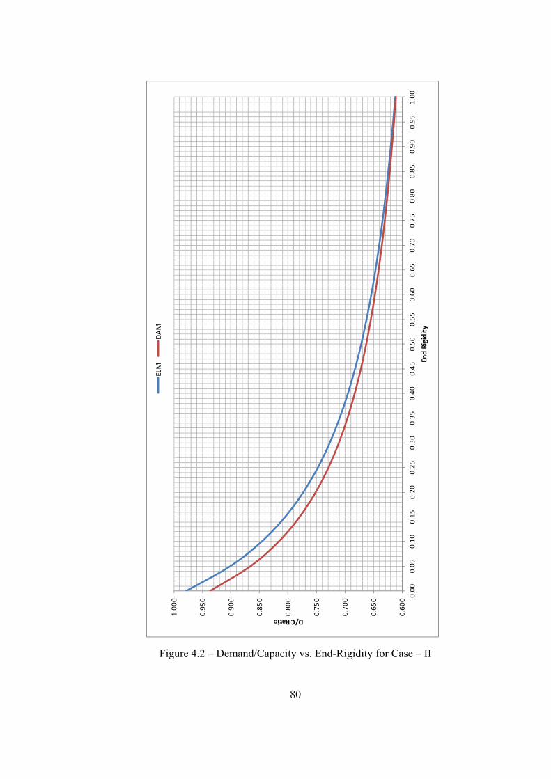
80
0.600
0.650
0.700
0.750
0.800
0.850
0.900
0.950
1.000
0.00
0.05
0.10
0.15
0.20
0.25
0.30
0.35
0.40
0.45
0.50
0.55
0.60
0.65
0.70
0.75
0.80
0.85
0.90
0.95
1.00
D/C Ratio
End Rigidity
ELM
DAM
Figure 4.2 – Demand/Capacity vs. End-Rigidity for Case – II
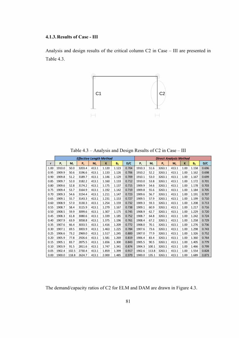
81
4.1.3. Results of Case - III
Analysis and design results of the critical column C2 in Case – III are presented in
Table 4.3.
Table 4.3 – Analysis and Design Results of C2 in Case – III
The demand/capacity ratios of C2 for ELM and DAM are drawn in Figure 4.3.
C1 C2
r Pr Mr Pc Mc K B2 D/C Pr Mr Pc Mc K B2 D/C
1.00 1910.0 50.0 3203.4 413.1 1.120 1.123 0.704 1910.3 51.6 3263.1 413.1 1.00 1.158 0.696
0.95 1909.9 50.6 3196.6 413.1 1.133 1.126 0.706 1910.2 52.2 3263.1 413.1 1.00 1.162 0.698
0.90 1909.8 51.2 3189.7 413.1 1.146 1.129 0.709 1910.1 53.0 3263.1 413.1 1.00 1.167 0.699
0.85 1909.7 52.0 3182.2 413.1 1.160 1.133 0.712 1910.0 53.8 3263.1 413.1 1.00 1.172 0.701
0.80 1909.6 52.8 3174.2 413.1 1.175 1.137 0.715 1909.9 54.6 3263.1 413.1 1.00 1.178 0.703
0.75 1909.4 53.7 3164.9 413.1 1.192 1.142 0.719 1909.8 55.6 3263.1 413.1 1.00 1.184 0.705
0.70 1909.3 54.6 3154.4 413.1 1.211 1.147 0.723 1909.6 56.7 3263.1 413.1 1.00 1.191 0.707
0.65 1909.1 55.7 3143.3 413.1 1.231 1.153 0.727 1909.5 57.9 3263.1 413.1 1.00 1.199 0.710
0.60 1908.9 57.0 3130.3 413.1 1.254 1.159 0.732 1909.3 59.3 3263.1 413.1 1.00 1.208 0.713
0.55 1908.7 58.4 3115.9 413.1 1.279 1.167 0.738 1909.1 60.9 3263.1 413.1 1.00 1.217 0.716
0.50 1908.5 59.9 3099.6 413.1 1.307 1.175 0.745 1908.9 62.7 3263.1 413.1 1.00 1.229 0.720
0.45 1908.3 61.8 3080.6 413.1 1.339 1.185 0.752 1908.7 64.8 3263.1 413.1 1.00 1.242 0.724
0.40 1907.9 63.9 3058.8 413.1 1.375 1.196 0.761 1908.4 67.2 3263.1 413.1 1.00 1.258 0.729
0.35 1907.6 66.4 3033.5 413.1 1.416 1.209 0.772 1908.0 70.1 3263.1 413.1 1.00 1.276 0.736
0.30 1907.1 69.5 3003.9 413.1 1.463 1.225 0.784 1907.6 73.6 3263.1 413.1 1.00 1.298 0.743
0.25 1906.6 73.2 2969.0 413.1 1.517 1.245 0.800 1907.0 77.9 3263.1 413.1 1.00 1.326 0.752
0.20 1905.9 77.8 2926.6 413.1 1.581 1.269 0.819 1906.4 83.4 3263.1 413.1 1.00 1.360 0.764
0.15 1905.1 83.7 2875.5 413.1 1.656 1.300 0.843 1905.5 90.5 3263.1 413.1 1.00 1.405 0.779
0.10 1903.9 91.5 2811.6 413.1 1.747 1.341 0.874 1904.3 100.1 3263.1 413.1 1.00 1.466 0.799
0.05 1902.4 102.5 2730.4 413.1 1.859 1.399 0.917 1902.6 113.8 3263.1 413.1 1.00 1.554 0.828
0.00 1900.0 118.8 2624.7 413.1 2.000 1.485 0.979 1900.0 135.1 3263.1 413.1 1.00 1.689 0.873
Effective Length Method Direct Analysis Method
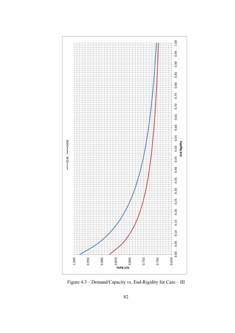
82
0.650
0.700
0.750
0.800
0.850
0.900
0.950
1.000
0.00
0.05
0.10
0.15
0.20
0.25
0.30
0.35
0.40
0.45
0.50
0.55
0.60
0.65
0.70
0.75
0.80
0.85
0.90
0.95
1.00
D/C Ratio
End Rigidity
ELM
DAM
Figure 4.3 – Demand/Capacity vs. End-Rigidity for Case – III

83
4.1.4. Results of Case - IV
Analysis and design results of critical columns C3 (interior) and C4 (exterior) in
Case – IV are presented in this part.
4.1.4.1. Results of C3 (Interior Column)
Table 4.4 - Analysis and Design Results of C3 (interior column) in Case – IV
The demand/capacity ratios of C3 for ELM and DAM are drawn in Figure 4.4.
C1 C2 C3 C4
r Pr Mr Pc Mc K B2 D/C Pr Mr Pc Mc K B2 D/C
1.00 553.8 160.4 3234.9 413.1 1.058 1.033 0.474 553.8 161.7 3263.1 413.1 1.00 1.041 0.476
0.95 553.5 161.2 3233.4 413.1 1.061 1.033 0.476 553.6 162.6 3263.1 413.1 1.00 1.042 0.478
0.90 553.3 162.1 3229.4 413.1 1.069 1.034 0.478 553.4 163.5 3263.1 413.1 1.00 1.042 0.480
0.85 553.1 163.1 3224.9 413.1 1.078 1.034 0.481 553.2 164.5 3263.1 413.1 1.00 1.043 0.483
0.80 552.9 164.2 3219.8 413.1 1.088 1.035 0.483 553.0 165.6 3263.1 413.1 1.00 1.044 0.486
0.75 552.7 165.4 3216.3 413.1 1.095 1.036 0.486 552.8 166.9 3263.1 413.1 1.00 1.045 0.489
0.70 552.6 166.8 3210.1 413.1 1.107 1.036 0.490 552.6 168.3 3263.1 413.1 1.00 1.046 0.492
0.65 552.4 168.4 3206.0 413.1 1.115 1.037 0.494 552.4 170.0 3263.1 413.1 1.00 1.047 0.496
0.60 552.2 170.2 3199.2 413.1 1.128 1.038 0.498 552.2 171.9 3263.1 413.1 1.00 1.048 0.501
0.55 552.0 172.3 3190.2 413.1 1.145 1.039 0.504 552.0 174.0 3263.1 413.1 1.00 1.050 0.506
0.50 551.8 174.8 3180.6 413.1 1.163 1.041 0.510 551.8 176.6 3263.1 413.1 1.00 1.051 0.512
0.45 551.6 177.7 3170.9 413.1 1.181 1.042 0.517 551.7 179.6 3263.1 413.1 1.00 1.054 0.519
0.40 551.5 181.3 3156.1 413.1 1.208 1.044 0.526 551.5 183.3 3263.1 413.1 1.00 1.056 0.528
0.35 551.3 185.6 3139.3 413.1 1.238 1.047 0.537 551.3 187.8 3263.1 413.1 1.00 1.059 0.539
0.30 551.1 191.0 3115.3 413.1 1.280 1.049 0.551 551.1 193.4 3263.1 413.1 1.00 1.063 0.553
0.25 550.9 198.0 3091.3 413.1 1.321 1.053 0.568 550.9 200.7 3263.1 413.1 1.00 1.067 0.570
0.20 550.7 207.3 3055.8 413.1 1.380 1.058 0.592 550.7 210.3 3263.1 413.1 1.00 1.074 0.594
0.15 550.5 220.3 3004.5 413.1 1.462 1.065 0.625 550.5 223.9 3263.1 413.1 1.00 1.082 0.626
0.10 550.3 239.7 2932.6 413.1 1.572 1.075 0.674 550.3 244.2 3263.1 413.1 1.00 1.095 0.676
0.05 550.1 271.6 2823.0 413.1 1.731 1.091 0.755 550.1 277.9 3263.1 413.1 1.00 1.116 0.757
0.00 550.0 333.5 2624.7 413.1 2.000 1.122 0.927 550.0 343.9 3263.1 413.1 1.00 1.157 0.917
Effective Length Method Direct Analysis Method
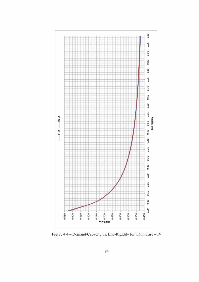
84
0.450
0.500
0.550
0.600
0.650
0.700
0.750
0.800
0.850
0.900
0.950
0.00
0.05
0.10
0.15
0.20
0.25
0.30
0.35
0.40
0.45
0.50
0.55
0.60
0.65
0.70
0.75
0.80
0.85
0.90
0.95
1.00
D/C Ratio
End Rigidity
ELM
DAM
Figure 4.4 – Demand/Capacity vs. End-Rigidity for C3 in Case – IV
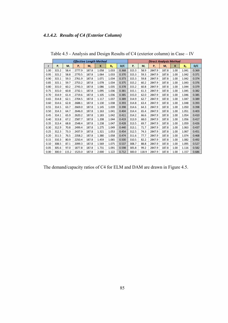
85
4.1.4.2. Results of C4 (Exterior Column)
Table 4.5 - Analysis and Design Results of C4 (exterior column) in Case – IV
The demand/capacity ratios of C4 for ELM and DAM are drawn in Figure 4.5.
r Pr Mr Pc Mc K B2 D/C Pr Mr Pc Mc K B2 D/C
1.00 315.2 58.4 2777.9 187.8 1.058 1.033 0.368 315.3 58.9 2847.9 187.8 1.00 1.041 0.369
0.95 315.2 58.8 2770.5 187.8 1.064 1.033 0.370 315.3 59.3 2847.9 187.8 1.00 1.042 0.371
0.90 315.1 59.3 2761.9 187.8 1.071 1.034 0.373 315.3 59.8 2847.9 187.8 1.00 1.042 0.374
0.85 315.1 59.7 2753.2 187.8 1.078 1.034 0.375 315.2 60.2 2847.9 187.8 1.00 1.043 0.376
0.80 315.0 60.2 2743.3 187.8 1.086 1.035 0.378 315.2 60.8 2847.9 187.8 1.00 1.044 0.379
0.75 315.0 60.8 2732.1 187.8 1.095 1.036 0.381 315.1 61.3 2847.9 187.8 1.00 1.045 0.382
0.70 314.9 61.4 2719.6 187.8 1.105 1.036 0.385 315.0 62.0 2847.9 187.8 1.00 1.046 0.385
0.65 314.8 62.1 2704.5 187.8 1.117 1.037 0.389 314.9 62.7 2847.9 187.8 1.00 1.047 0.389
0.60 314.6 62.8 2688.1 187.8 1.130 1.038 0.393 314.8 63.4 2847.9 187.8 1.00 1.048 0.393
0.55 314.5 63.7 2669.0 187.8 1.145 1.039 0.398 314.6 64.3 2847.9 187.8 1.00 1.050 0.398
0.50 314.3 64.7 2646.0 187.8 1.163 1.041 0.404 314.4 65.4 2847.9 187.8 1.00 1.051 0.403
0.45 314.1 65.9 2620.2 187.8 1.183 1.042 0.411 314.2 66.6 2847.9 187.8 1.00 1.054 0.410
0.40 313.8 67.2 2587.7 187.8 1.208 1.044 0.419 313.9 68.0 2847.9 187.8 1.00 1.056 0.417
0.35 313.4 68.8 2548.4 187.8 1.238 1.047 0.428 313.5 69.7 2847.9 187.8 1.00 1.059 0.426
0.30 312.9 70.8 2499.4 187.8 1.275 1.049 0.440 313.1 71.7 2847.9 187.8 1.00 1.063 0.437
0.25 312.3 73.3 2437.9 187.8 1.321 1.053 0.454 312.5 74.3 2847.9 187.8 1.00 1.067 0.451
0.20 311.5 76.5 2358.2 187.8 1.380 1.058 0.474 311.6 77.7 2847.9 187.8 1.00 1.074 0.468
0.15 310.3 80.9 2250.4 187.8 1.459 1.065 0.500 310.5 82.2 2847.9 187.8 1.00 1.082 0.492
0.10 308.5 87.1 2099.3 187.8 1.569 1.075 0.537 308.7 88.8 2847.9 187.8 1.00 1.095 0.527
0.05 305.6 97.0 1877.8 187.8 1.731 1.091 0.598 305.8 99.2 2847.9 187.8 1.00 1.116 0.582
0.00 300.0 115.2 1523.0 187.8 2.000 1.122 0.712 300.0 118.9 2847.9 187.8 1.00 1.157 0.686
Effective Length Method Direct Analysis Method

86
0.350
0.400
0.450
0.500
0.550
0.600
0.650
0.700
0.750
0.00
0.05
0.10
0.15
0.20
0.25
0.30
0.35
0.40
0.45
0.50
0.55
0.60
0.65
0.70
0.75
0.80
0.85
0.90
0.95
1.00
D/C Ratio
End Rigidity
ELM
DAM
Figure 4.5 – Demand/Capacity vs. End-Rigidity for C4 in Case – IV
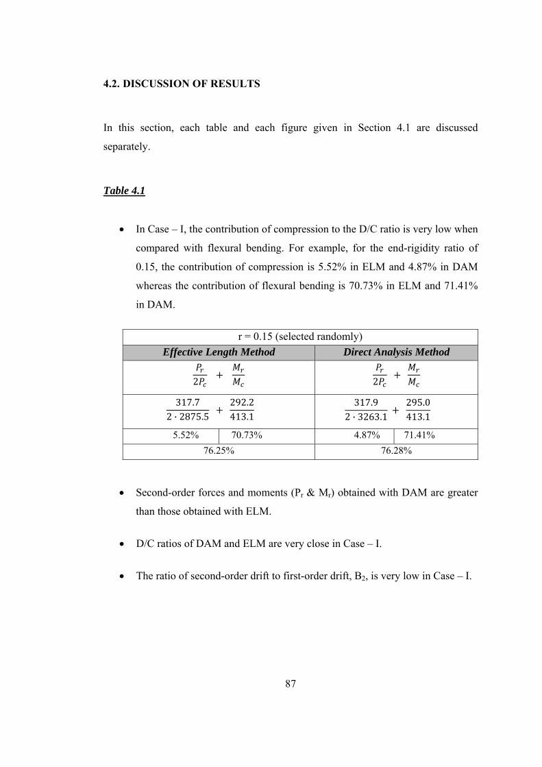
87
4.2. DISCUSSION OF RESULTS
In this section, each table and each figure given in Section 4.1 are discussed
separately.
Table 4.1
In Case – I, the contribution of compression to the D/C ratio is very low when
compared with flexural bending. For example, for the end-rigidity ratio of
0.15, the contribution of compression is 5.52% in ELM and 4.87% in DAM
whereas the contribution of flexural bending is 70.73% in ELM and 71.41%
in DAM.
r = 0.15 (selected randomly)
Effective Length Method Direct Analysis Method
2
2
317.72 · 2875.5
292.2413.1
317.9
2 · 3263.1
295.0413.1
5.52% 70.73% 4.87% 71.41%
76.25% 76.28%
Second-order forces and moments (Pr & Mr) obtained with DAM are greater
than those obtained with ELM.
D/C ratios of DAM and ELM are very close in Case – I.
The ratio of second-order drift to first-order drift, B2, is very low in Case – I.

88
Figure 4.1
The effect of flexible connections is better observed in the figure than the
table. In the pinned connected case (r = 0.00) the D/C ratio is about 0.95
whereas in rigidly connected case (r = 1.00) the D/C ratio is about 0.53 for
both methods. Between end-rigidity values of 1.00 and 0.50 the increase in
the D/C ratio is not significant, it rises from 0.53 to 0.61 for both methods.
However, between end-rigidity values of 0.50 and 0.00 the increase in the
D/C ratio is significant. It increases from 0.61 to 0.95 for both methods.
Table 4.2
In Case – II, the contribution of compression to the D/C ratio is lower than
the contribution of flexural bending but close to it. For example, for the end-
rigidity ratio of 0.15, the contribution of compression is 35.22% in ELM and
31.05% in DAM whereas the contribution of flexural bending is 45.32% in
ELM and 46.95% in DAM.
r = 0.15 (selected randomly)
Effective Length Method Direct Analysis Method
89·
89·
1012.82875.5
89·210.6413.1
1013.23263.1
89·218.2413.1
35.22% 45.32% 31.05% 46.95% 80.54% 78.00%
Second-order forces and moments (Pr & Mr) obtained with DAM are greater
than those obtained with ELM.
D/C ratios of DAM and ELM are close to each other however as r factor
approaches to 0.00, the D/C ratios become different in Case – II.

89
The ratio of second-order drift to first-order drift, B2, is average in Case – II.
Figure 4.2
In pinned connected case (r = 0.00) the D/C ratio is 0.98 for ELM and 0.94
for DAM whereas in rigidly connected case (r = 1.00) the D/C ratio is about
0.61 for both methods. Between end-rigidity values of 1.00 and 0.50, the
increase in the D/C ratio is not significant; it rises from 0.61 to 0.67 for ELM
and to 0.66 for DAM. However, between end-rigidity values of 0.50 and 0.00
the increase in the D/C ratio is significant. It increases from 0.67 to 0.98 for
ELM and it increases from 0.66 to 0.94 for DAM.
Table 4.3
In Case – III, the contribution of compression to the D/C ratio is greater than
the contribution of flexural bending. For example, for the end-rigidity ratio of
0.15, the contribution of compression is 66.25% in ELM and 58.40% in DAM
whereas the contribution of flexural bending is 18.01% in ELM and 19.47%
in DAM.
r = 0.15 (selected randomly)
Effective Length Method Direct Analysis Method
89·
89·
1905.12875.5
89·83.7413.1
1905.53263.1
89·90.5413.1
66.25% 18.01% 58.40% 19.47% 84.26% 77.87%
Second-order forces and moments (Pr & Mr) obtained with DAM are greater
than those obtained with ELM.
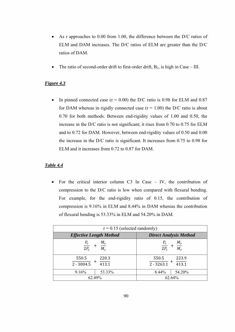
90
As r approaches to 0.00 from 1.00, the difference between the D/C ratios of
ELM and DAM increases. The D/C ratios of ELM are greater than the D/C
ratios of DAM.
The ratio of second-order drift to first-order drift, B2, is high in Case – III.
Figure 4.3
In pinned connected case (r = 0.00) the D/C ratio is 0.98 for ELM and 0.87
for DAM whereas in rigidly connected case (r = 1.00) the D/C ratio is about
0.70 for both methods. Between end-rigidity values of 1.00 and 0.50, the
increase in the D/C ratio is not significant; it rises from 0.70 to 0.75 for ELM
and to 0.72 for DAM. However, between end-rigidity values of 0.50 and 0.00
the increase in the D/C ratio is significant. It increases from 0.75 to 0.98 for
ELM and it increases from 0.72 to 0.87 for DAM.
Table 4.4
For the critical interior column C3 In Case – IV, the contribution of
compression to the D/C ratio is low when compared with flexural bending.
For example, for the end-rigidity ratio of 0.15, the contribution of
compression is 9.16% in ELM and 8.44% in DAM whereas the contribution
of flexural bending is 53.33% in ELM and 54.20% in DAM.
r = 0.15 (selected randomly)
Effective Length Method Direct Analysis Method
2
2
550.52 · 3004.5
220.3413.1
550.5
2 · 3263.1
223.9413.1
9.16% 53.33% 8.44% 54.20% 62.49% 62.64%

91
Second-order forces and moments (Pr & Mr) obtained with DAM are greater
than those obtained with ELM.
D/C ratios of DAM and ELM are very close for the interior column C3 in
Case – IV.
The ratio of second-order drift to first-order drift, B2, is low in Case – IV.
Figure 4.4
In the pinned connected case (r = 0.00) the D/C ratio is about 0.92 whereas in
rigidly connected case (r = 1.00) the D/C ratio is about 0.47 for both methods.
Between end-rigidity values of 1.00 and 0.50 the increase in the D/C ratio is
not significant, it rises from 0.47 to 0.51 for both methods. However, between
end-rigidity values of 0.50 and 0.00 the increase in the D/C ratio is
significant. It increases from 0.51 to 0.92 for both methods.
Table 4.5
For the critical exterior column C4 In Case – IV, the contribution of
compression to the D/C ratio is low when compared with flexural bending.
For example, for the end-rigidity ratio of 0.15, the contribution of
compression is 6.89% in ELM and 5.45% in DAM whereas the contribution
of flexural bending is 43.08% in ELM and 43.77% in DAM.
r = 0.15 (selected randomly)
Effective Length Method Direct Analysis Method
2
2
310.32 · 2250.4
80.9187.8
310.5
2 · 2847.9
82.2187.8
6.89% 43.08% 5.45% 43.77% 49.97% 49.22%
92
Second-order forces and moments (Pr & Mr) obtained with DAM are greater
than those obtained with ELM.
D/C ratios of DAM and ELM are close for the exterior column C4 in Case –
IV.
The ratio of second-order drift to first-order drift, B2, is low in Case – IV.
Figure 4.5
In the pinned connected case (r = 0.00) the D/C ratio is about 0.70 whereas in
rigidly connected case (r = 1.00) the D/C ratio is about 0.37 for both methods.
Between end-rigidity values of 1.00 and 0.50 the increase in the D/C ratio is
not significant, it rises from 0.37 to 0.40 for both methods. However, between
end-rigidity values of 0.50 and 0.00 the increase in the D/C ratio is
significant. It increases from 0.40 to 0.70. Between r values of 0.00 and 0.25
(where the effective length factor begins to increase significantly) it is
observed that DAM becomes slightly unconservative when compared with
ELM. At r equals to 0.25 the D/C ratio is 0.45 for both methods. At r equals
to 0.00 the D/C ratio for ELM is 0.71 and for DAM it is 0.69.
93
CHAPTER 5
CONCLUSIONS AND FUTURE RECOMMENDATIONS
5.1. CONCLUSIONS
To compare DAM and ELM in semi-rigid frames and to investigate the effect of
semi-rigid joints to stability, four case studies were conducted and the results of these
cases were obtained in terms of the demand/capacity ratio. The results were
presented and discussed in Chapter 4. Based on these discussions, following
conclusions were obtained.
In Case – I, the contribution of compression to D/C ratio is very low and
accordingly the results of ELM and DAM are very close. In Case – II, the
contribution of compression increases and accordingly ELM becomes more
conservative than DAM. In Case – III, the D/C ratios are governed by
compression therefore the difference between ELM and DAM becomes large.
When comparing Case – I, Case – II and Case – III, it is concluded that as the
contribution of compression to D/C ratio increases, the D/C ratios obtained
with ELM become greater than the D/C ratios obtained with DAM. This
means that as the compressive force increases ELM gives conservative results
when compared with DAM.
ELM underestimates the internal forces and moments when compared with
DAM since geometric imperfections and member inelasticity are not
accounted for in the analysis whereas DAM considers these in the analysis.
To compensate the underestimation of internal forces and moments, ELM
decreases the compressive strength of members by using effective length

94
factors. In cases where ELM and DAM give similar design results for the
members, the internal forces obtained with ELM are lower than the forces
obtained with DAM and this creates problem in connection design. The
connections are designed with smaller forces and moments with ELM.
Connection design is very important and critical for steel design since the fail
of a connection may lead the fail of the entire structure therefore, design of
connections with smaller forces than required is an undesired and
unacceptable situation.
From the results of the exterior column in Case – IV it is observed that in
minor-axis bending, DAM becomes slightly unconservative when compared
with ELM between the end-rigidity factor range of 0.00 and 0.25. This
conclusion is also obtained in the study of Ziemian and Martinez-Garcia [1].
As the end-rigidity factor approaches from 0.25 to 0.00, the influence of
semi-rigid connections becomes more significant and this is reflected by the
effective length factors in ELM. Since the influence of effective length factor
on the compressive strength is more pronounced in minor-axis bending in
general, the compressive strength of the members decreases more than it
decreases in major axis bending within this end-rigidity range.
From the results of all cases, it is observed that between end-rigidity values of
0.00 and 0.50, the connection stiffness significantly affects the D/C ratios
whereas between 0.50 and 1.00 it loses its influence. If the structure is
designed assuming the joints are ideally pinned (end-rigidity values is zero),
the structure will have more capacity than the calculated since the
connections are not perfectly pinned. In other words, small moment capacity
of the connections may increase the resistance of the structure significantly if
the connections are designed as pinned. This means that economy can be
provided by using semi-rigid connections instead of pinned connections. If
the structure is designed assuming the joints are fully rigid, the actual
capacity of the structure will be less than the calculated. In this case, an

95
unsafe design comes out. However if the connections are designed as semi-
rigid instead of fully rigid, safety of the design is guaranteed with a little bit
increase in the cost of the structure. The increase in the cost is low because
within the end-rigidity range of 0.50-1.00 the increase in the demand/capacity
ratio is small.

96
5.2. FUTURE RECOMMENDATIONS
The followings are recommended for future studies:
One may perform the analyses assuming column bases semi-rigid instead of
fully rigid to determine the influence of column bases to the stability of the
structure.
Model the semi-rigid connections as non-linear instead of linear modeling to
obtain more realistic results.
Model a 3-D structure to investigate the effect of stability methods on major-
axis or minor-axis bending of columns.

97
REFERENCES
[1] Ziemian, R.D., Martinez-Garcia, J.M., “Frame Studies to Compare Stability Provisions Appearing in the 2005 AISC Specification”, Stability and Ductility of Steel Structures, Lisbon, 2006.
[2] Surovek, A.E., Ziemian, R.D., “The Direct Analysis Method: Bridging the Gap from Linear Elastic Analysis to Advanced Analysis in Steel Frame Design”, Structures Congress, New York, April 2005.
[3] Prajzner, J., “Evaluation of the Effective Length Method and the Direct Analysis Method for the Design of Steel Columns in Frame Structures”, University of Maryland, Maryland, 2006.
[4] Surovek, A.E., White, D.W., Leon, R.T., “Direct Analysis for Design Evaluation of Partially Restrained Steel Framing Systems”, Journal of Structural Engineering, September 2005.
[5] Kartal, M.E., Başağa, H.B., Bayraktar, A., Muvafık, M., “Effects of Semi-Rigid Connection on Structural Response”, Electronic Journal of Structural Engineering (10), 2010.
[6] Monforton, G.R., Wu, T.S., “Matrix Analysis of Semi-Rigidly Connected Frames”, Journal of Structural Division, ASCE, 89, ST6, 13-42, 1963.
[7] Xu, L., “Critical Buckling Loads of Semi-Rigid Steel Frames”, University of Waterloo.
[8] Patodi, S.C., Chauhan, J.M., “First Order Analysis of Plane Frames with Semi-Rigid Connections”, National Conference on Recent Trends in Engineering & Technology, Gujarat, 13-14 May 2011.
[9] Mathur, K., “Effects of Residual Stresses and Initial Imperfections on Earthquake Response of Steel Moment Frames”, Master Thesis, University of Illinois, Illinois, 2011.
[10] Deierlein, G., “Background and Illustrative Examples on Proposed Direct Analysis Method for Stability Design of Moment Frames”, Report on Behalf of AISC TC10, July 2003.
98
[11] Yura, J.A., “The Effective Length of Columns in Unbraced Frames”, AISC Engineering Journal, 1971.
[12] Chen, W.F., Lui, E.M., “Stability Design of Steel Frames”, CRC Press, Florida, 1991.
[13] AISC (American Institute of Steel Construction), “Specification for Structural Steel Buildings”, Chicago, 2010
[14] AISC (American Institute of Steel Construction), “Specification for Structural Steel Buildings”, Chicago, 2005
[15] Carter, C.J., Geschwindner, L.F., “A Comparison of Frame Stability Analysis Methods in ANSI/AISC 360-05”
[16] Eröz, M., White, D.W., DesRoches, R., “Direct Analysis and Design of Steel Frames Accounting for Partially Restrained Column Base Conditions”, Journal of Structural Engineering, 1508-1517, September 2008.
[17] Galambos, T.V., Surovek, A.E., “Structural Stability of Steel: Concepts and Applications for Structural Engineers”, John Wiley & Sons, Inc., New Jersey, 2008.
[18] Geschwindner, L.F., Disque, R.O., “Flexible Moment Connections for Unbraced Frames Subject to Lateral Forces – A Return to Simplicity”, Engineering Journal / Second Quarter, 99-112, 2005.
[19] Gönen, H., Ünlüoğlu, E., “Frames with Semirigid Structural Connections”, Journal of Engineering Sciences, Pamukkale University, 1998.
[20] Hayalioğlu, M.S., Değertekin, S.Ö., Görgün, H., “Design of Semi-Rigid Planar Steel Frames According to Turkish Steel Design Code”, Sigma: Journal of Engineering and Natural Sciences (2), 2004.
[21] Hibbeler, R.C., “Structural Analysis (Sixth Edition)”, Pearson Prentice Hall, New Jersey, 2006.
[22] Nair, R.S., “Stability Analysis and the 2005 AISC Specification”, The Steel Conference, New Orleans, 18-21 April 2007.
99
[23] Seçer, M., “The Effect of Flexible Joints on the Effective Length Factor and Critical Elastic Buckling Load of Unbraced Steel Columns”, Journal of Dumlupınar University Institute of Natural Sciences, May 2006.
[24] White, D.W., Surovek, A.E., Alemdar, B.N., Changi C.J., Kim, Y.D., Kuchenbecker, G.H “Stability Analysis and Design of Steel Building Frames Using the 2005 AISC Specification”, Steel Structures 6, 71-91, 2006.

100
APPENDIX A
FLEXURAL STRENGTH OF COLUMNS
a) Flexural Strength of Columns in Case – I, Case – II and Case – III
In-plane flexural strength of a column is determined according to Chapter F of the
AISC 360-10. First, the compactness of HEA300 should be checked. The limiting
values are given in Table B4.1b of AISC 360-10 which is given in Table A1.
Table A1 – Compactness Limits

101
Compactness Check of Flanges
0.38 0.38200000345
9.15 1.0 1.0200000345
24.08
300/214
10.71 0.38 1.0
Compactness Check of Web
3.76 3.76200000345
90.53 5.70 1.0200000345
137.2
290 14 · 28.5
30.8 3.76 5.7
Flexural Strength (According to Chapter F.3 of AISC 360-10)
i. Lateral Torsional Buckling
4000
1.76 · · 1.76 · 74.7 ·200000345
3165
1.95 · ·0.7
··
··
6.760.7
10868
Where
E = 200000 MPa
Fy = 345 MPa

102
J = 878000 mm4
c = 1
Sx = 1259310 mm3
Iy = 63100000 mm4
290 14 276
·4
631 10 · 2764
1.202 10
· √631 10 · 1.202 101259310
83.15
3165 4000 10868
· 345 · 1383000 477 ·
0.7
2.213 · 4.77 10 4.77 10 0.7 · 345 · 12593104000 316510868 3165
M 1014 ·
1014 · 477 · 477 ·
Where Cb is calculated as;
12.52.5 3 4 3
12.5 · 209.72.5 · 209.7 3 · 58.1 4 · 31.2 3 · 120.4
C 2.213
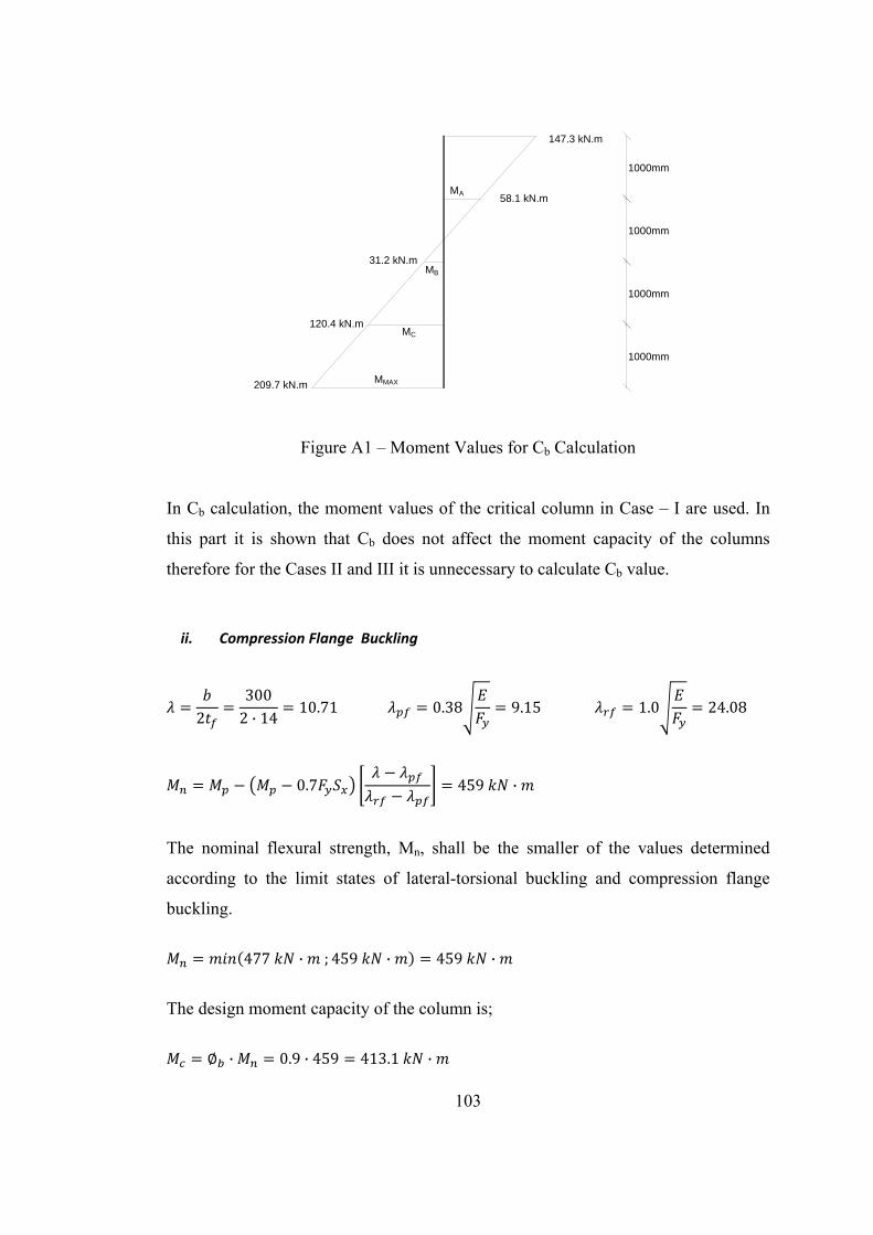
103
Figure A1 – Moment Values for Cb Calculation
In Cb calculation, the moment values of the critical column in Case – I are used. In
this part it is shown that Cb does not affect the moment capacity of the columns
therefore for the Cases II and III it is unnecessary to calculate Cb value.
ii. Compression Flange Buckling
23002 · 14
10.71 0.38 9.15 1.0 24.08
0.7 459 ·
The nominal flexural strength, Mn, shall be the smaller of the values determined
according to the limit states of lateral-torsional buckling and compression flange
buckling.
477 · ; 459 · 459 ·
The design moment capacity of the column is;
· 0.9 · 459 413.1 ·
147.3 kN.m
58.1 kN.m
1000mm
1000mm
1000mm
1000mm
MA
MB
MC
31.2 kN.m
120.4 kN.m
209.7 kN.m MMAX
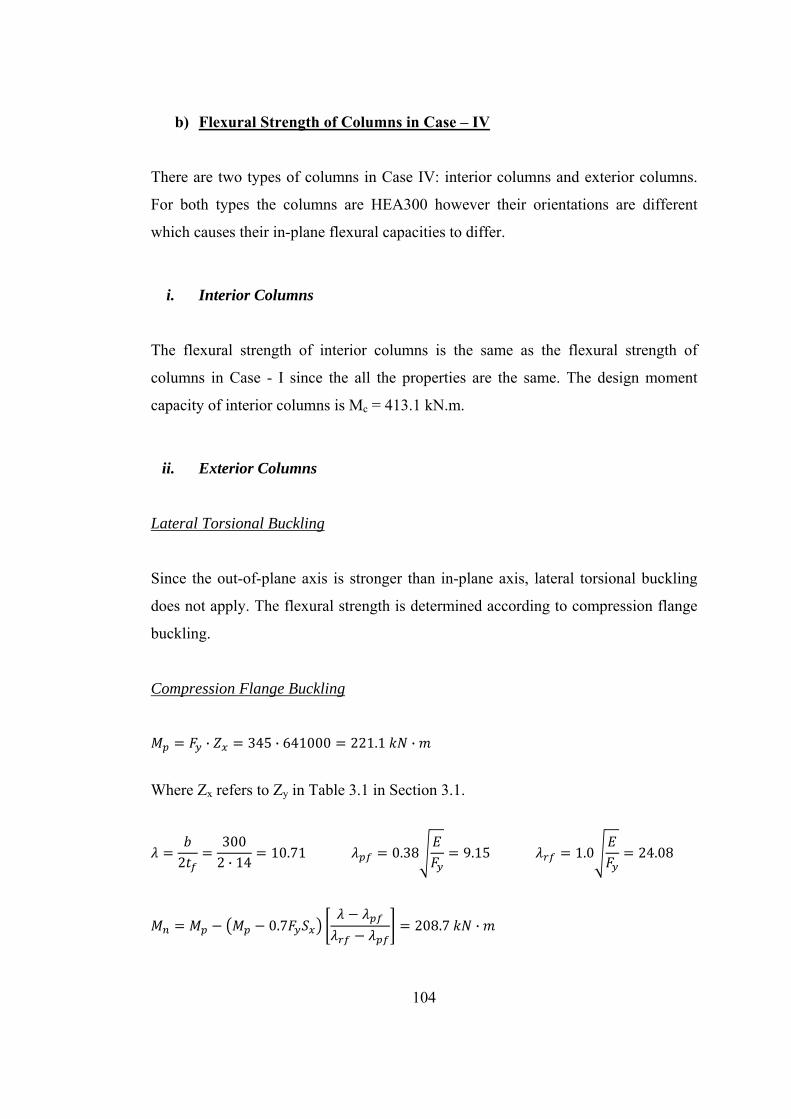
104
b) Flexural Strength of Columns in Case – IV
There are two types of columns in Case IV: interior columns and exterior columns.
For both types the columns are HEA300 however their orientations are different
which causes their in-plane flexural capacities to differ.
i. Interior Columns
The flexural strength of interior columns is the same as the flexural strength of
columns in Case - I since the all the properties are the same. The design moment
capacity of interior columns is Mc = 413.1 kN.m.
ii. Exterior Columns
Lateral Torsional Buckling
Since the out-of-plane axis is stronger than in-plane axis, lateral torsional buckling
does not apply. The flexural strength is determined according to compression flange
buckling.
Compression Flange Buckling
· 345 · 641000 221.1 ·
Where Zx refers to Zy in Table 3.1 in Section 3.1.
23002 · 14
10.71 0.38 9.15 1.0 24.08
0.7 208.7 ·

105
The design moment capacity of the column is;
· 0.9 · 208.7 187.8 ·

106
APPENDIX B
COMPRESSIVE STRENGTH OF COLUMNS
a) Compressive Strength of Columns in Case – I, Case – II and Case – III
i. Design with ELM
Compressive strength of the columns is determined according to Chapter E of AISC
360-10. The physical properties of HEA300 are given in Section 3.1 and the effective
length factor of the column is calculated as 1.193 in Section 3.2.1.2. The calculated
effective length factor is for the in-plane buckling, the out-of-plane effective length is
assumed as 0.5 in assumption 6 in Section 3.1.
1.193 127.1 1.193 · 4000
127.137.5
0.500 74.7 0.5 · 400074.7
26.8
37.5
4.71 4.71200000345
113.4 37.5
0.658 0.658 345 311.1

107
20000037.5
1403
· 311.1 · 11300 3515
· 0.9 · 3515 3164
Available axial strength of the column is Pc = 3164 kN.
ii. Design with DAM
The physical properties of HEA300 are given in Section 3.1, the in-plane effective
length factor of the column is 1.0 and the out-of-plane effective length factor is 0.5 as
specified in Section 3.1.
1.0 127.1 1.0 · 4000127.1
31.5
0.5 74.7 0.5 · 400074.7
26.8
31.5
4.71 4.71200000345
113.4 31.5
0.658 0.658 345 320.8
20000037.5
1989

108
· 320.8 · 11300 3625
· 0.9 · 3625 3263
Available axial strength of the column is Pc = 3263 kN.
b) Compressive Strength of Columns in Case – IV
i. Interior Columns
Design with ELM
Compressive strength of the columns is determined according to Chapter E of AISC
360-10. The physical properties of HEA300 are given in Section 3.1 and the effective
length factor of the column is calculated as 1.095 in Section 3.5.1.2. The calculated
effective length factor is for the in-plane buckling, the out-of-plane effective length is
assumed as 0.5 in assumption 6 in Section 3.1.
1.095 127.1 1.095 · 4000
127.134.5
0.500 74.7 0.5 · 400074.7
26.8
34.5
4.71 4.71200000345
113.4 34.5
0.658 0.658 345 316.2

109
20000034.5
1658
· 316.2 · 11300 3573
· 0.9 · 3573 3216
Available axial strength of the column is Pc = 3216 kN.
Design with DAM
The interior columns in Case - IV have the same properties with those of columns in
Case I (both of them are HEA300, have 4m length and effective length factor of
1.00) therefore interior columns in Case - IV (C2 & C3) have the same compressive
strength with the columns in Case - I.
Available axial strength of the interior columns is Pc = 3263 kN.
ii. Exterior Columns
Design with ELM
The only difference between the interior and exterior columns is the orientation. The
flexural strength of exterior columns is calculated in the same way with the interior
columns however the physical properties given for x-direction is accepted as they are
for y-direction and the properties given for y are for x-direction.
1.095 74.7 1.095 · 4000
74.758.5
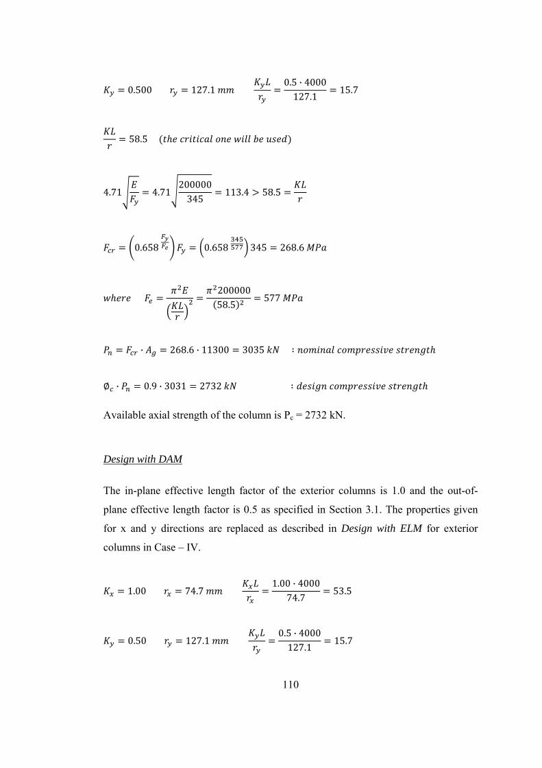
110
0.500 127.1 0.5 · 4000127.1
15.7
58.5
4.71 4.71200000345
113.4 58.5
0.658 0.658 345 268.6
20000058.5
577
· 268.6 · 11300 3035
· 0.9 · 3031 2732
Available axial strength of the column is Pc = 2732 kN.
Design with DAM
The in-plane effective length factor of the exterior columns is 1.0 and the out-of-
plane effective length factor is 0.5 as specified in Section 3.1. The properties given
for x and y directions are replaced as described in Design with ELM for exterior
columns in Case – IV.
1.00 74.7 1.00 · 4000
74.753.5
0.50 127.1 0.5 · 4000127.1
15.7

111
53.5
4.71 4.71200000345
113.4 53.5
0.658 0.658 345 280.0
20000053.5
688
· 280.0 · 11300 3164
· 0.9 · 3164 2848
Available axial strength of the column is Pc = 2848 kN.

112
APPENDIX C
STRUCTURAL ANALYSIS STEPS OF CASES
1. Case - II
a) Design with ELM
Stiffness matrix of the columns C1 and C2,
5.65 10 0 0 5.65 10 0 0
0 6.85 10 1.37 10 0 6.85 10 1.37 10
0 1.37 10 3.65 10 0 1.37 10 1.83 10
5.65 10 0 0 5.65 10 0 0
0 6.85 10 1.37 10 0 6.85 10 1.37 10
0 1.37 10 1.83 10 0 1.37 10 3.65 10
Displacement matrices of columns C1 and C2,
000
000
Stiffness matrix of the beam B1,
1.36 10 5.42 10 1.36 10 5.42 10
5.42 10 3.15 10 5.42 10 1.18 10
1.36 10 5.42 10 1.36 10 5.42 10
5.42 10 1.18 10 5.42 10 3.15 10

113
Displacement matrix of beam B1,
The connection stiffness and stability functions are calculated as,
1
13 0.75
1
13 · 2 · 10 · 482 · 10
8000 ·
1.085 · 10 ·
14
14 4
14 · 2 · 10 · 482 · 108000 · 1.085 · 10
2 · 10 · 482 · 108000
41.085 · 10
2.037
412
412 · 2 · 10 · 482 · 108000 · 1.085 · 10
2.0372.62
412
412 · 2 · 10 · 482 · 108000 · 1.085 · 10
2.0372.62
2 22.037
0.98

114
Member forces for C1 is (units are in kN and m),
5.65 10 0 0 5.65 10 0 0
0 6.85 10 1.37 10 0 6.85 10 1.37 10
0 1.37 10 3.65 10 0 1.37 10 1.83 10
5.65 10 0 0 5.65 10 0 0
0 6.85 10 1.37 10 0 6.85 10 1.37 10
0 1.37 10 1.83 10 0 1.37 10 3.65 10
1.7279
12.7947
0.0022
0
0
0
976.3
57.5
94.9
976.3
57.5
135.1
Member forces for C2 is (units are in kN and m),
5.65 10 0 0 5.65 10 0 0
0 6.85 10 1.37 10 0 6.85 10 1.37 10
0 1.37 10 3.65 10 0 1.37 10 1.83 10
5.65 10 0 0 5.65 10 0 0
0 6.85 10 1.37 10 0 6.85 10 1.37 10
0 1.37 10 1.83 10 0 1.37 10 3.65 10
1.8119
12.7947
0.0022
0
0
0
1023.7
57.5
94.9
1023.7
57.5
135.1
Member forces for B1 is (units are in kN and m),
1.36 10 5.42 10 1.36 10 5.42 10
5.42 10 3.15 10 5.42 10 1.18 10
1.36 10 5.42 10 1.36 10 5.42 10
5.42 10 1.18 10 5.42 10 3.15 10
1.7279
0.0022
1.8119
0.0022
23.7
94.9
23.7
94.9

115
b) Design with DAM
Stiffness matrix of the columns C1 and C2,
4.52 10 0 0 4.52 10 0 0
0 5.48 10 1.10 10 0 5.48 10 1.10 10
0 1.10 10 2.92 10 0 1.10 10 1.46 10
4.52 10 0 0 4.52 10 0 0
0 5.48 10 1.10 10 0 5.48 10 1.10 10
0 1.10 10 1.46 10 0 1.10 10 2.92 10
Displacement matrices of columns C1 and C2,
000
000
Stiffness matrix of the beam B1,
1.08 10 4.34 10 1.08 10 4.34 10
4.34 10 2.52 10 4.34 10 9.46 10
1.08 10 4.34 10 1.08 10 4.34 10
4.34 10 9.46 10 4.34 10 2.52 10
Displacement matrix of beam B1,
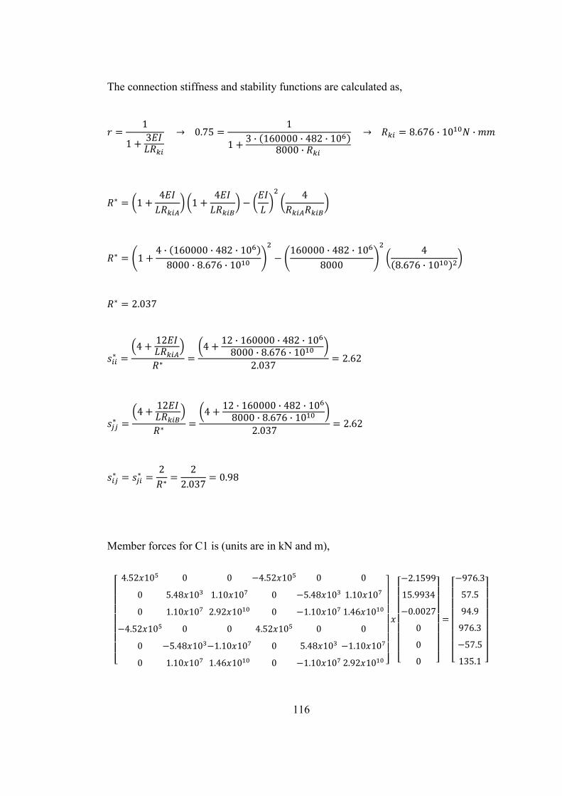
116
The connection stiffness and stability functions are calculated as,
1
13 0.75
1
13 · 160000 · 482 · 10
8000 ·
8.676 · 10 ·
14
14 4
14 · 160000 · 482 · 108000 · 8.676 · 10
160000 · 482 · 108000
48.676 · 10
2.037
412
412 · 160000 · 482 · 108000 · 8.676 · 10
2.0372.62
412
412 · 160000 · 482 · 108000 · 8.676 · 10
2.0372.62
2 22.037
0.98
Member forces for C1 is (units are in kN and m),
4.52 10 0 0 4.52 10 0 0
0 5.48 10 1.10 10 0 5.48 10 1.10 10
0 1.10 10 2.92 10 0 1.10 10 1.46 10
4.52 10 0 0 4.52 10 0 0
0 5.48 10 1.10 10 0 5.48 10 1.10 10
0 1.10 10 1.46 10 0 1.10 10 2.92 10
2.1599
15.9934
0.0027
0
0
0
976.3
57.5
94.9
976.3
57.5
135.1

117
Member forces for C2 is (units are in kN and m),
4.52 10 0 0 4.52 10 0 0
0 5.48 10 1.10 10 0 5.48 10 1.10 10
0 1.10 10 2.92 10 0 1.10 10 1.46 10
4.52 10 0 0 4.52 10 0 0
0 5.48 10 1.10 10 0 5.48 10 1.10 10
0 1.10 10 1.46 10 0 1.10 10 2.92 10
2.2649
15.9934
0.0027
0
0
0
1023.7
57.5
94.9
1023.7
57.5
135.1
Member forces for B1 is (units are in kN and m),
1.08 10 4.34 10 1.08 10 4.34 10
4.34 10 2.52 10 4.34 10 9.46 10
1.08 10 4.34 10 1.08 10 4.34 10
4.34 10 9.46 10 4.34 10 2.52 10
2.1599
0.0027
2.2649
0.0027
23.7
94.9
23.7
94.9

118
2. Case - III
a) Design with ELM
Stiffness matrix of the columns C1 and C2,
5.65 10 0 0 5.65 10 0 0
0 6.85 10 1.37 10 0 6.85 10 1.37 10
0 1.37 10 3.65 10 0 1.37 10 1.83 10
5.65 10 0 0 5.65 10 0 0
0 6.85 10 1.37 10 0 6.85 10 1.37 10
0 1.37 10 1.83 10 0 1.37 10 3.65 10
Displacement matrices of columns C1 and C2,
000
000
Stiffness matrix of the beam B1,
1.36 10 5.42 10 1.36 10 5.42 10
5.42 10 3.15 10 5.42 10 1.18 10
1.36 10 5.42 10 1.36 10 5.42 10
5.42 10 1.18 10 5.42 10 3.15 10
Displacement matrix of beam B1,

119
The connection stiffness and stability functions are calculated as,
1
13 0.75
1
13 · 2 · 10 · 482 · 10
8000 ·
1.085 · 10 ·
14
14 4
14 · 2 · 10 · 482 · 108000 · 1.085 · 10
2 · 10 · 482 · 108000
41.085 · 10
2.037
412
412 · 2 · 10 · 482 · 108000 · 1.085 · 10
2.0372.62
412
412 · 2 · 10 · 482 · 108000 · 1.085 · 10
2.0372.62
2 22.037
0.98

120
Member forces for C1 is (units are in kN and m),
5.65 10 0 0 5.65 10 0 0
0 6.85 10 1.37 10 0 6.85 10 1.37 10
0 1.37 10 3.65 10 0 1.37 10 1.83 10
5.65 10 0 0 5.65 10 0 0
0 6.85 10 1.37 10 0 6.85 10 1.37 10
0 1.37 10 1.83 10 0 1.37 10 3.65 10
3.3482
4.4503
0.0008
0
0
0
1891.7
20.0
33.0
1891.7
20.0
47.0
Member forces for C2 is (units are in kN and m),
5.65 10 0 0 5.65 10 0 0
0 6.85 10 1.37 10 0 6.85 10 1.37 10
0 1.37 10 3.65 10 0 1.37 10 1.83 10
5.65 10 0 0 5.65 10 0 0
0 6.85 10 1.37 10 0 6.85 10 1.37 10
0 1.37 10 1.83 10 0 1.37 10 3.65 10
3.3774
4.4503
0.0008
0
0
0
1908.3
20.0
33.0
1908.3
20.0
47.0
Member forces for B1 is (units are in kN and m),
1.36 10 5.42 10 1.36 10 5.42 10
5.42 10 3.15 10 5.42 10 1.18 10
1.36 10 5.42 10 1.36 10 5.42 10
5.42 10 1.18 10 5.42 10 3.15 10
3.3482
0.0008
3.3774
0.0008
8.3
33.0
8.3
33.0
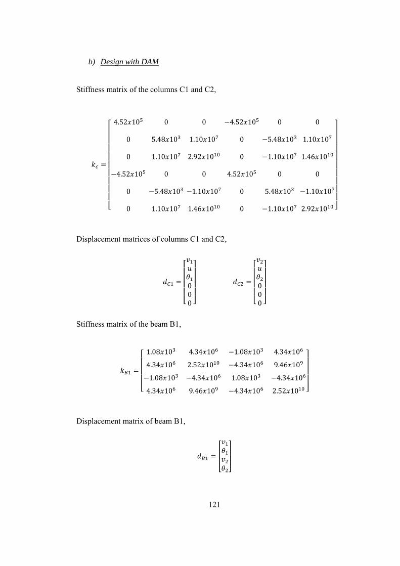
121
b) Design with DAM
Stiffness matrix of the columns C1 and C2,
4.52 10 0 0 4.52 10 0 0
0 5.48 10 1.10 10 0 5.48 10 1.10 10
0 1.10 10 2.92 10 0 1.10 10 1.46 10
4.52 10 0 0 4.52 10 0 0
0 5.48 10 1.10 10 0 5.48 10 1.10 10
0 1.10 10 1.46 10 0 1.10 10 2.92 10
Displacement matrices of columns C1 and C2,
000
000
Stiffness matrix of the beam B1,
1.08 10 4.34 10 1.08 10 4.34 10
4.34 10 2.52 10 4.34 10 9.46 10
1.08 10 4.34 10 1.08 10 4.34 10
4.34 10 9.46 10 4.34 10 2.52 10
Displacement matrix of beam B1,

122
The connection stiffness and stability functions are calculated as,
1
13 0.75
1
13 · 160000 · 482 · 10
8000 ·
8.676 · 10 ·
14
14 4
14 · 160000 · 482 · 108000 · 8.676 · 10
160000 · 482 · 108000
48.676 · 10
2.037
412
412 · 160000 · 482 · 108000 · 8.676 · 10
2.0372.62
412
412 · 160000 · 482 · 108000 · 8.676 · 10
2.0372.62
2 22.037
0.98
Member forces for C1 is (units are in kN and m),
4.52 10 0 0 4.52 10 0 0
0 5.48 10 1.10 10 0 5.48 10 1.10 10
0 1.10 10 2.92 10 0 1.10 10 1.46 10
4.52 10 0 0 4.52 10 0 0
0 5.48 10 1.10 10 0 5.48 10 1.10 10
0 1.10 10 1.46 10 0 1.10 10 2.92 10
4.1853
5.5629
0.0010
0
0
0
1891.7
20.0
33.0
1891.7
20.0
47.0
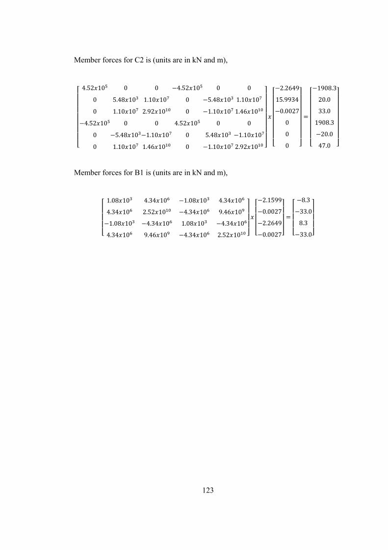
123
Member forces for C2 is (units are in kN and m),
4.52 10 0 0 4.52 10 0 0
0 5.48 10 1.10 10 0 5.48 10 1.10 10
0 1.10 10 2.92 10 0 1.10 10 1.46 10
4.52 10 0 0 4.52 10 0 0
0 5.48 10 1.10 10 0 5.48 10 1.10 10
0 1.10 10 1.46 10 0 1.10 10 2.92 10
2.2649
15.9934
0.0027
0
0
0
1908.3
20.0
33.0
1908.3
20.0
47.0
Member forces for B1 is (units are in kN and m),
1.08 10 4.34 10 1.08 10 4.34 10
4.34 10 2.52 10 4.34 10 9.46 10
1.08 10 4.34 10 1.08 10 4.34 10
4.34 10 9.46 10 4.34 10 2.52 10
2.1599
0.0027
2.2649
0.0027
8.3
33.0
8.3
33.0

124
3. Case - IV
a) Design with ELM
Stiffness matrix of the columns C1 and C4,
5.65 10 0 0 5.65 10 0 0
0 2.37 10 4.73 10 0 2.37 10 4.73 10
0 4.73 10 1.26 10 0 4.73 10 6.31 10
5.65 10 0 0 5.65 10 0 0
0 2.37 10 4.73 10 0 2.37 10 4.73 10
0 4.73 10 6.31 10 0 4.73 10 1.26 10
Stiffness matrix of the columns C2 and C3,
5.65 10 0 0 5.65 10 0 0
0 6.85 10 1.37 10 0 6.85 10 1.37 10
0 1.37 10 3.65 10 0 1.37 10 1.83 10
5.65 10 0 0 5.65 10 0 0
0 6.85 10 1.37 10 0 6.85 10 1.37 10
0 1.37 10 1.83 10 0 1.37 10 3.65 10
Displacement matrices of columns C1, C2, C3 and C4,
000
000
000
000
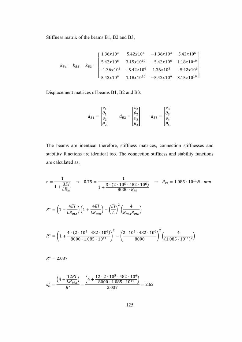
125
Stiffness matrix of the beams B1, B2 and B3,
1.36 10 5.42 10 1.36 10 5.42 10
5.42 10 3.15 10 5.42 10 1.18 10
1.36 10 5.42 10 1.36 10 5.42 10
5.42 10 1.18 10 5.42 10 3.15 10
Displacement matrices of beams B1, B2 and B3:
The beams are identical therefore, stiffness matrices, connection stiffnesses and
stability functions are identical too. The connection stiffness and stability functions
are calculated as,
1
13 0.75
1
13 · 2 · 10 · 482 · 10
8000 ·
1.085 · 10 ·
14
14 4
14 · 2 · 10 · 482 · 108000 · 1.085 · 10
2 · 10 · 482 · 108000
41.085 · 10
2.037
412
412 · 2 · 10 · 482 · 108000 · 1.085 · 10
2.0372.62

126
412
412 · 2 · 10 · 482 · 108000 · 1.085 · 10
2.0372.62
2 22.037
0.98
Member forces for C1 (units are in kN and m);
5.65 10 0 0 5.65 10 0 0
0 2.37 10 4.73 10 0 2.37 10 4.73 10
0 4.73 10 1.26 10 0 4.73 10 6.31 10
5.65 10 0 0 5.65 10 0 0
0 2.37 10 4.73 10 0 2.37 10 4.73 10
0 4.73 10 6.31 10 0 4.73 10 1.26 10
0.5062
13.739
0.0011
0
0
0
286.0
27.3
51.1
286.0
27.3
58.1
Member forces for C2 (units are in kN and m);
5.65 10 0 0 5.65 10 0 0
0 6.85 10 1.37 10 0 6.85 10 1.37 10
0 1.37 10 3.65 10 0 1.37 10 1.83 10
5.65 10 0 0 5.65 10 0 0
0 6.85 10 1.37 10 0 6.85 10 1.37 10
0 1.37 10 1.83 10 0 1.37 10 3.65 10
0.9680
13.739
0.0016
0
0
0
546.9
72.2
129.8
546.9
72.2
159.0
Member forces for C3 (units are in kN and m);
5.65 10 0 0 5.65 10 0 0
0 6.85 10 1.37 10 0 6.85 10 1.37 10
0 1.37 10 3.65 10 0 1.37 10 1.83 10
5.65 10 0 0 5.65 10 0 0
0 6.85 10 1.37 10 0 6.85 10 1.37 10
0 1.37 10 1.83 10 0 1.37 10 3.65 10
0.9781
13.739
0.0016
0
0
0
552.6
72.8
131.3
552.6
72.8
159.7

127
Member forces for C4 (units are in kN and m);
5.65 10 0 0 5.65 10 0 0
0 2.37 10 4.73 10 0 2.37 10 4.73 10
0 4.73 10 1.26 10 0 4.73 10 6.31 10
5.65 10 0 0 5.65 10 0 0
0 2.37 10 4.73 10 0 2.37 10 4.73 10
0 4.73 10 6.31 10 0 4.73 10 1.26 10
0.5062
13.739
0.0011
0
0
0
314.5
27.8
52.4
314.5
27.8
58.7
Member forces for B1 (units are in kN and m);
1.36 10 5.42 10 1.36 10 5.42 10
5.42 10 3.15 10 5.42 10 1.18 10
1.36 10 5.42 10 1.36 10 5.42 10
5.42 10 1.18 10 5.42 10 3.15 10
0.5062
0.0011
0.9680
0.0016
14.0
51.1
14.0
61.0
Member forces for B2 (units are in kN and m);
1.36 10 5.42 10 1.36 10 5.42 10
5.42 10 3.15 10 5.42 10 1.18 10
1.36 10 5.42 10 1.36 10 5.42 10
5.42 10 1.18 10 5.42 10 3.15 10
0.9680
0.0016
0.9781
0.0016
17.1
68.8
17.1
68.0
Member forces for B3 (units are in kN and m);
1.36 10 5.42 10 1.36 10 5.42 10
5.42 10 3.15 10 5.42 10 1.18 10
1.36 10 5.42 10 1.36 10 5.42 10
5.42 10 1.18 10 5.42 10 3.15 10
0.9781
0.0016
0.5566
0.0010
14.5
63.3
14.5
52.4

128
b) Design with DAM
Stiffness matrix of the columns C1 and C4:
4.52 10 0 0 4.52 10 0 0
0 1.89 10 3.79 10 0 1.89 10 3.79 10
0 3.79 10 1.01 10 0 3.79 10 5.05 10
4.52 10 0 0 4.52 10 0 0
0 1.89 10 3.79 10 0 1.89 10 3.79 10
0 3.79 10 5.05 10 0 3.79 10 1.01 10
Stiffness matrix of the columns C2 and C3:
4.52 10 0 0 4.52 10 0 0
0 5.48 10 1.10 10 0 5.48 10 1.10 10
0 1.10 10 2.92 10 0 1.10 10 1.46 10
4.52 10 0 0 4.52 10 0 0
0 5.48 10 1.10 10 0 5.48 10 1.10 10
0 1.10 10 1.46 10 0 1.10 10 2.92 10
Displacement matrices of columns C1, C2, C3 and C4:
000
000
000
000
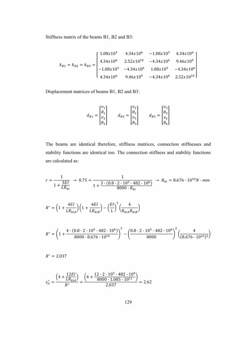
129
Stiffness matrix of the beams B1, B2 and B3:
1.08 10 4.34 10 1.08 10 4.34 10
4.34 10 2.52 10 4.34 10 9.46 10
1.08 10 4.34 10 1.08 10 4.34 10
4.34 10 9.46 10 4.34 10 2.52 10
Displacement matrices of beams B1, B2 and B3:
The beams are identical therefore, stiffness matrices, connection stiffnesses and
stability functions are identical too. The connection stiffness and stability functions
are calculated as:
1
13 0.75
1
13 · 0.8 · 2 · 10 · 482 · 10
8000 ·
8.676 · 10 ·
14
14 4
14 · 0.8 · 2 · 10 · 482 · 10
8000 · 8.676 · 100.8 · 2 · 10 · 482 · 10
80004
8.676 · 10
2.037
412
412 · 2 · 10 · 482 · 108000 · 1.085 · 10
2.0372.62
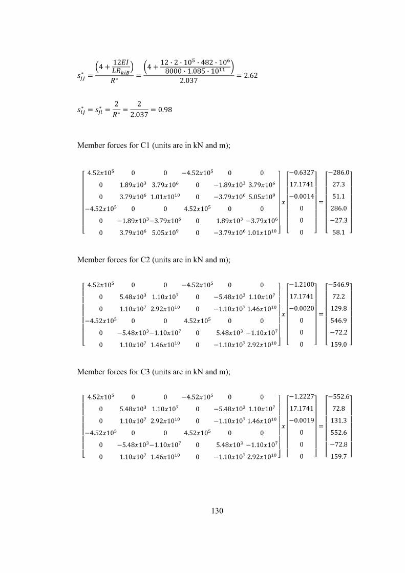
130
412
412 · 2 · 10 · 482 · 108000 · 1.085 · 10
2.0372.62
2 22.037
0.98
Member forces for C1 (units are in kN and m);
4.52 10 0 0 4.52 10 0 0
0 1.89 10 3.79 10 0 1.89 10 3.79 10
0 3.79 10 1.01 10 0 3.79 10 5.05 10
4.52 10 0 0 4.52 10 0 0
0 1.89 10 3.79 10 0 1.89 10 3.79 10
0 3.79 10 5.05 10 0 3.79 10 1.01 10
0.6327
17.1741
0.0014
0
0
0
286.0
27.3
51.1
286.0
27.3
58.1
Member forces for C2 (units are in kN and m);
4.52 10 0 0 4.52 10 0 0
0 5.48 10 1.10 10 0 5.48 10 1.10 10
0 1.10 10 2.92 10 0 1.10 10 1.46 10
4.52 10 0 0 4.52 10 0 0
0 5.48 10 1.10 10 0 5.48 10 1.10 10
0 1.10 10 1.46 10 0 1.10 10 2.92 10
1.2100
17.1741
0.0020
0
0
0
546.9
72.2
129.8
546.9
72.2
159.0
Member forces for C3 (units are in kN and m);
4.52 10 0 0 4.52 10 0 0
0 5.48 10 1.10 10 0 5.48 10 1.10 10
0 1.10 10 2.92 10 0 1.10 10 1.46 10
4.52 10 0 0 4.52 10 0 0
0 5.48 10 1.10 10 0 5.48 10 1.10 10
0 1.10 10 1.46 10 0 1.10 10 2.92 10
1.2227
17.1741
0.0019
0
0
0
552.6
72.8
131.3
552.6
72.8
159.7
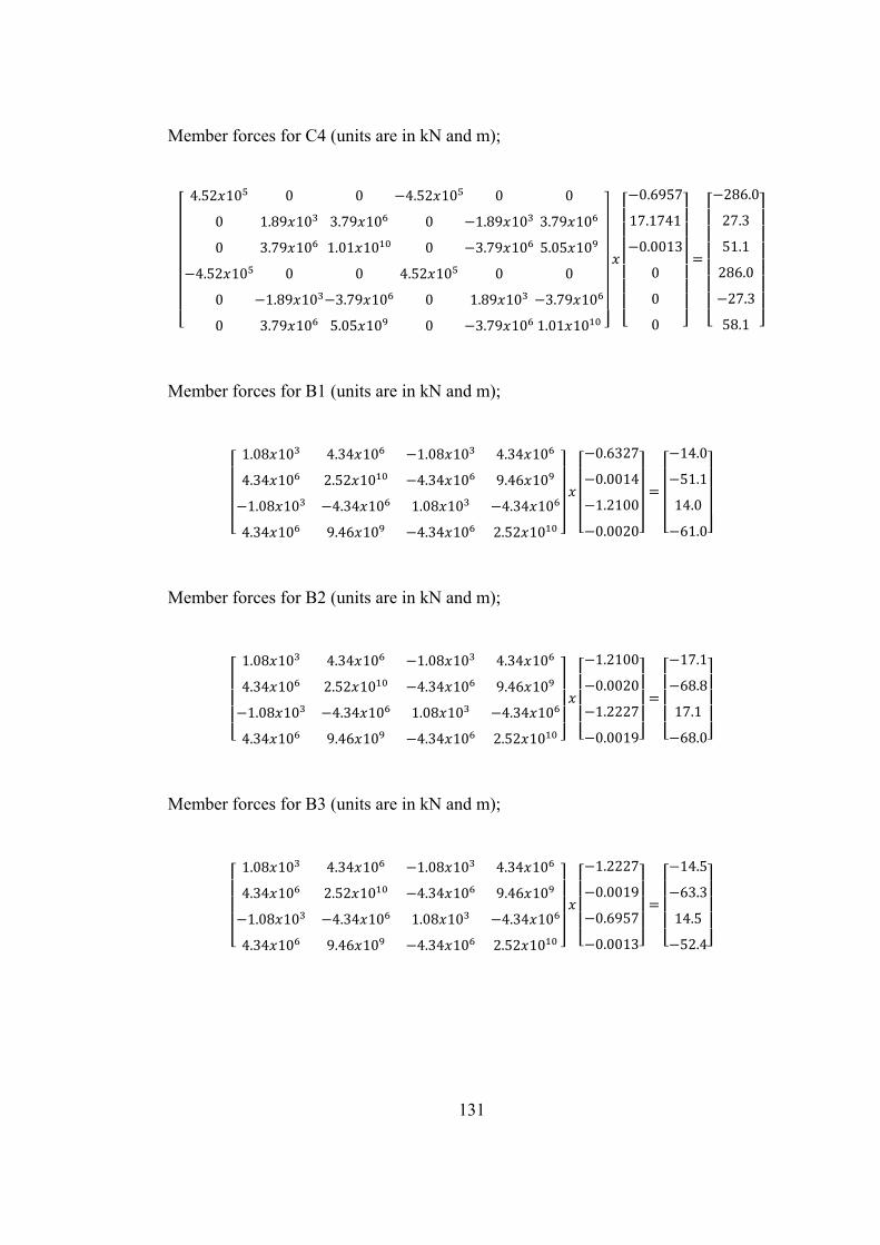
131
Member forces for C4 (units are in kN and m);
4.52 10 0 0 4.52 10 0 0
0 1.89 10 3.79 10 0 1.89 10 3.79 10
0 3.79 10 1.01 10 0 3.79 10 5.05 10
4.52 10 0 0 4.52 10 0 0
0 1.89 10 3.79 10 0 1.89 10 3.79 10
0 3.79 10 5.05 10 0 3.79 10 1.01 10
0.6957
17.1741
0.0013
0
0
0
286.0
27.3
51.1
286.0
27.3
58.1
Member forces for B1 (units are in kN and m);
1.08 10 4.34 10 1.08 10 4.34 10
4.34 10 2.52 10 4.34 10 9.46 10
1.08 10 4.34 10 1.08 10 4.34 10
4.34 10 9.46 10 4.34 10 2.52 10
0.6327
0.0014
1.2100
0.0020
14.0
51.1
14.0
61.0
Member forces for B2 (units are in kN and m);
1.08 10 4.34 10 1.08 10 4.34 10
4.34 10 2.52 10 4.34 10 9.46 10
1.08 10 4.34 10 1.08 10 4.34 10
4.34 10 9.46 10 4.34 10 2.52 10
1.2100
0.0020
1.2227
0.0019
17.1
68.8
17.1
68.0
Member forces for B3 (units are in kN and m);
1.08 10 4.34 10 1.08 10 4.34 10
4.34 10 2.52 10 4.34 10 9.46 10
1.08 10 4.34 10 1.08 10 4.34 10
4.34 10 9.46 10 4.34 10 2.52 10
1.2227
0.0019
0.6957
0.0013
14.5
63.3
14.5
52.4

132
APPENDIX D
LATERAL DRIFT VALUES OF CASES
1. Case - I
Table D.1 – Lateral Drift Values for Case - I
r
1.00
0.95
0.90
0.85
0.80
0.75
0.70
0.65
0.60
0.55
0.50
0.45
0.40
0.35
0.30
0.25
0.20
0.15
0.10
0.05
0.00
55.81 59.13
63.89 68.29
25.11 25.76
25.96 26.66
26.91 27.66
21.38 21.86
21.88 22.37
22.42 22.93
23.00 23.55
23.64 24.22
24.34 24.95
41.47 43.28
45.16 47.32
49.80 52.43
33.87 35.07
35.98 37.33
38.47 40.02
29.16 30.05
30.52 31.49
32.08 33.15
27.97 28.78
53.89
31.76
34.33
37.50
41.51
46.75
23.89
25.03
26.34
27.86
29.64
19.86
20.50
21.21
22.00
22.89
1st Order Drift (mm)
17.11
17.50
17.93
18.40
18.91
19.47
20.09
20.77
21.53
22.38
23.33
24.42
25.66
30.78
33.18
36.13
39.84
44.64
27.10
28.78
51.11
2ndOrder Drift (mm)
Effective Length Method
1stOrder Drift (mm) 2
nd Order Drift (mm)
Direct Analysis Method
17.41
17.82
18.26
18.75
19.28

133
2. Case - II
Table D.2 – Lateral Drift Values for Case - II
r
1.00
0.95
0.90
0.85
0.80
0.75
0.70
0.65
0.60
0.55
0.50
0.45
0.40
0.35
0.30
0.25
0.20
0.15
0.10
0.05
0.00 33.59 40.56 41.99 53.47
26.18 30.23 32.73 39.30
29.34 34.52 36.67 45.14
21.80 24.54 27.25 31.67
23.74 27.02 29.68 34.99
18.91 20.94 23.64 26.89
20.22 22.56 25.28 29.04
16.86 18.45 21.08 23.63
17.81 19.59 22.26 25.12
15.33 16.64 19.17 21.25
16.05 17.48 20.06 22.35
14.15 15.25 17.68 19.44
14.70 15.90 18.38 20.29
13.20 14.16 16.50 18.02
13.65 14.67 17.06 18.69
12.43 13.27 15.53 16.87
12.79 13.69 15.99 17.42
11.78 12.54 14.73 15.93
12.09 12.89 15.11 16.38
11.24 11.93 14.05 15.14
11.50 12.22 14.38 15.52
Effective Length Method Direct Analysis Method
1st Order Drift (mm) 2
ndOrder Drift (mm) 1
stOrder Drift (mm) 2
nd Order Drift (mm)
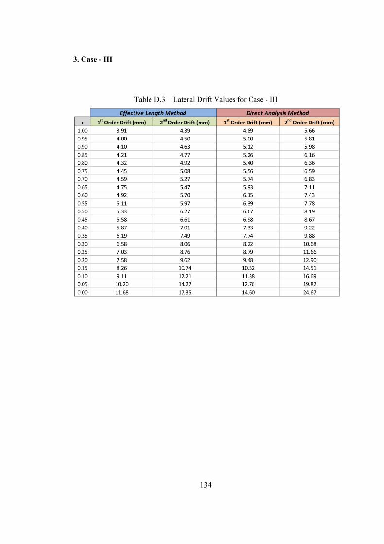
134
3. Case - III
Table D.3 – Lateral Drift Values for Case - III
r
1.00
0.95
0.90
0.85
0.80
0.75
0.70
0.65
0.60
0.55
0.50
0.45
0.40
0.35
0.30
0.25
0.20
0.15
0.10
0.05
0.00 11.68 17.35 14.60 24.67
9.11 12.21 11.38 16.69
10.20 14.27 12.76 19.82
7.58 9.62 9.48 12.90
8.26 10.74 10.32 14.51
6.58 8.06 8.22 10.68
7.03 8.76 8.79 11.66
5.87 7.01 7.33 9.22
6.19 7.49 7.74 9.88
5.33 6.27 6.67 8.19
5.58 6.61 6.98 8.67
4.92 5.70 6.15 7.43
5.11 5.97 6.39 7.78
4.59 5.27 5.74 6.83
4.75 5.47 5.93 7.11
4.32 4.92 5.40 6.36
4.45 5.08 5.56 6.59
4.10 4.63 5.12 5.98
4.21 4.77 5.26 6.16
3.91 4.39 4.89 5.66
4.00 4.50 5.00 5.81
Effective Length Method Direct Analysis Method
1st Order Drift (mm) 2
ndOrder Drift (mm) 1
stOrder Drift (mm) 2
nd Order Drift (mm)

135
4. Case - IV
Table D.4 – Lateral Drift Values for Case - IV
r
1.00
0.95
0.90
0.85
0.80
0.75
0.70
0.65
0.60
0.55
0.50
0.45
0.40
0.35
0.30
0.25
0.20
0.15
0.10
0.05
0.00 43.41 48.70 54.27 62.78
27.78 29.85 34.72 38.02
33.29 36.31 41.61 46.44
21.92 23.19 27.40 29.42
24.31 25.88 30.39 32.88
18.85 19.78 23.56 25.04
20.18 21.25 25.22 26.92
16.95 17.71 21.19 22.38
17.80 18.63 22.25 23.56
15.67 16.31 19.59 20.59
16.26 16.94 20.32 21.41
14.74 15.30 18.42 19.31
15.17 15.77 18.96 19.90
14.03 14.54 17.54 18.34
14.36 14.90 17.95 18.80
13.48 13.95 16.85 17.59
13.74 14.23 17.17 17.94
13.03 13.47 16.29 16.98
13.24 13.70 16.55 17.27
12.67 13.08 15.83 16.48
12.84 13.27 16.05 16.72
Effective Length Method Direct Analysis Method
1st Order Drift (mm) 2
ndOrder Drift (mm) 1
stOrder Drift (mm) 2
nd Order Drift (mm)