A COMPARATIVE STUDY OF THE TAIWAN AND JAPAN EQUITY …5)-277-297.pdf · A COMPARATIVE STUDY OF THE...

Asian Economic and Financial Review, 2016, 6(5): 277-297

277

† Corresponding author

DOI: 10.18488/journal.aefr/2016.6.5/102.5.277.297

ISSN(e): 2222-6737/ISSN(p): 2305-2147

© 2016 AESS Publications. All Rights Reserved.

A COMPARATIVE STUDY OF THE TAIWAN AND JAPAN EQUITY AND FOREIGN EXCHANGE MARKETS: MODELING, ESTIMATION AND APPLICATION OF THE COMPONENT GARCH-IN-MEAN MODEL

Hsiang-Hsi Liu1† --- Robin K Chou2

1 Distinguished Professor, Graduate Institute of International Business, National Taipei University, Taipei, Taiwan 2

Professor, Department of Finance, National Chengchi University, Taipei, Taiwan

ABSTRACT

The main purpose of this paper is to verify the effectiveness of the bivariate Component GARCH-in-mean (GARCH-

M) model and analyze the interactions and risk premium of equity markets by exploring the short- and long-run

volatility components on both the Taiwanese and Japanese equity markets. We show that unexpected shocks of

volatility will in general influence the fluctuations of both equity and foreign exchange markets. Persistence on the

long-run volatility components of both markets is also found. The results also reveal that the positive risk-return

relation on equity markets can be further verified when the impacts of short and long-run volatility components are

decomposed by the Component GARCH-M model. The decomposition can also facilitate reflecting the transitory and

permanent volatility impacts of foreign exchange exposure on the returns of equity markets.


Keywords: ARCH, Component GARCH-in-mean model (GARCH-M), Risk premium, Foreign currency exposure, Equity market, Transitory

and permanent volatilities.

JEL Classification: G1; C32; F31.

Contribution/ Originality

This study is one of very few studies which have investigated risk premium and the interactions between equity

markets, by exploring the short- and long-run volatility components on both the Taiwanese and Japanese equity and

foreign exchange markets via estimating bivariate Component GARCH-in-mean (GARCH-M) mode.

1. INTRODUCTION

It is widely believed that exchange rates affect the value of assets. Exchange rates are one of the major sources of

uncertainty, being that they are typically four times as volatile as interest rates. The analysis of the correlation

between equity returns and foreign exchange rates has received much attention in financial econometric studies in

recent years. The ways of modeling these financial time series have been enriched by standard GARCH processes.

However, when capturing the long-term and short-term volatility effects, how to choose an appropriate model is a

complicated problem. It has been observed in the literature that volatility effects may be better modeled using a

Component GARCH-M model. To consider the permanent and transitory effects of the impact on rate of returns and

Asian Economic and Financial Review

ISSN(e): 2222-6737/ISSN(p): 2305-2147

URL: www.aessweb.com

http://crossmark.crossref.org/dialog/?doi=10.18488/journal.aefr/2016.6.5/102.5.277.297

http://crossmark.crossref.org/dialog/?doi=10.18488/journal.aefr/2016.6.5/102.5.277.297


278


the effects of short- and long-run volatility components on both Taiwanese and Japanese equity markets, this paper

adopts the Component GARCH-M model developed by Engle and Lee (1999).

Considering that Taiwan and Japan have a close interaction both economically and financially In South-East

Asia, Taiwan and Japan’s economic model may play a part in their respective exchange rate risk. It is important to

note that Taiwan and Japan have a close relationship on trades and investments, and thus exchange rates can

potentially influence both side’s capital and equity markets. And furthermore reduce the risk reduction for portfolio

investment. The purpose of this paper is to verify the effectiveness of the bivariate Component GARCH-M model and

analyze the risk premium of equity markets by exploring the effects of the short and long-run volatility components

on both Taiwanese and Japanese equity markets. Under the Component GARCH-M framework, time series effects of

volatility are decomposed into short and long-run volatility components. The estimated model reveals that there is a

rich interaction between the rates of return for both the Taiwan and Japan equity markets. The Component GARCH-

M model appropriately captures the effect of foreign currency exposure on the volatility of equity markets.

Furthermore, it also better delineates the effect of equity shocks on the volatility of equity markets.

This paper is organized as follows. The literature review is presented in section 2, followed by section 3, where a

theoretical framework of the Component GARCH-M model is presented. The data and variables definitions are

described in section 4. Section 4 also presents empirical results of this study. Section 5 concludes this article.

2. LITERATURE REVIEW

Traditional econometric models have a constant one-period forecast variance. Engle (1982) generalized this setup

and develops a new class of econometric processes called autoregressive conditional heteroscedastic (ARCH)

processes. Time-varying volatility is not only important in forecasting future market movements but is also central to

a variety of financial issues, such as portfolio design, risk management, and derivative pricing. Although it is

common to find a significant statistical relationship between current volatility and lagged volatilities, it is generally

difficult to decide the exact models that appropriately capture the inter-temporal dependencies observed on the data

series. Bollerslev (1986) generalizes the ARCH framework introduced by Engle (1982) into the GARCH framework,

where it incorporates past conditional variances into current conditional variance, In his study, stationary conditions

and autocorrelation structures of the GARCH model for this new class of parametric models are derived, furthermore,

maximum likelihood estimation and testing procedures are also considered.

Engle et al. (1987) continue to extend the ARCH model into the ARCH-in-Mean (ARCH-M) model, in which the

conditional mean is an explicit function of the conditional variance of the ARCH-M process. Since the ARCH in

mean model can deal with the trade-off of the risk-return profile in finance research, it causes a boom of finance

research on the time-varying conditional variance. When the volatility of financial asset returns changes, agents

naturally suspect that time-varying risk premia may be operative. Later on Lee (1999) also applies the multivariate

component model for conditional asset return covariance, which is an extension of the invariant volatility component

model. The conditional covariance is divided into a long-run (trend) component and a short-run (transitory)

component. Through the decomposition, the long-run correlation and volatility co-persistence can be studied

separately. Through their research, Christoffersen et al. (2008) proposed a model with the volatility of returns

consisting of two components. One is a long-run component, which can be modeled as fully persistent, and the other

is a short-run component that has a zero mean. The model can be viewed as a refined version of Engle and Lee (1999)

allowing for easy valuation of European options.

Watanabe and Harada (2006) examine the effects of Bank of Japan's (BOJ) intervention on the volatility and the

level of the yen/dollar exchange rate. Specifically, the conventional GARCH model and the component GARCH

model, where the volatility consists of short-run and long-run components, are estimated using the BOJ's and the


279


Federal Reserve’s system intervention data. Results based on the component GARCH model show new evidence on

the effects of the BOJ's intervention on the volatility of the yen/dollar exchange rate. Yau and Nieh (2009) investigate

the exchange rate effects of the New Taiwan Dollar against the Japanese Yen on stock prices in Japan and Taiwan by

the threshold error correction model (TECM). The finding suggests that there is a long run equilibrium relationship

between NTD/JPY and the stock prices of Japan and Taiwan. However in the short run, the results of TECM Granger

causality tests show that no short run causal relationships exist between the two financial assets considered for both

countries` cases. Recently, Lee et al. (2010) adopt the Component GARCH model to examine the relationships

between volatility and trading volume in five major Asian index futures markets. Their empirical results confirm that

the volatility of stock index futures in Asian markets includes permanent and transitory components. Also, the

information conveyance in these markets is not very efficient.

In general, regarding emerging markets around the East-Asia region not quite much research has been done on

the interactive effects of the stock and foreign exchange markets regarding the view of the short- and long-run

volatility components by the Component GARCH model. Some researches refer to the connections between the stock

and foreign exchange markets through the spillovers of market volatility by GARCH-type models or via linear or

even nonlinear co-integration analysis. Even though both the GARCH model (focused on market volatility spillovers)

and the co-integration analysis (focused on the co-integration vector variation of the long-term correlation after

exogenous chocks), these methods still cannot help to detect the impacts of information transmission on the

permanent and transitory return volatility between the stock and foreign exchange markets. In light of such short- and

long-run characteristics of return volatility, our study applies the Component GARCH model, modified from the

traditional GARCH model by Engle and Lee (1999) that decomposes conditional variance into permanent and

transitory components.

3. THEORETICAL FRAMEWORK

3.1. The Framework of Component GARCH Model

To explore the short- and long-run volatility components and interactions on Taiwanese and Japanese equity with

foreign exchange markets, this article proposes an application and extension of the univariate Component GARCH

model developed by Engle and Lee (1999). The framework of the Component GARCH model is as follows:

ttt xy ),0(~| 1 ttt hN (1)

1

2

1 ttt hh (2)

Where ty is a covariance-stationary process; tx includes the regressors; t is the information set available at

time t; and th is a conditional variance measurable in respect to 1t . The multi-step-ahead forecast of conditional

variance is denoted as )|( 1 tktkt yVarh . Assuming 1 , the multi-step-ahead forecast of conditional

variance under GARCH (1, 1) framework is

11k

kth

1 as k (3)


280


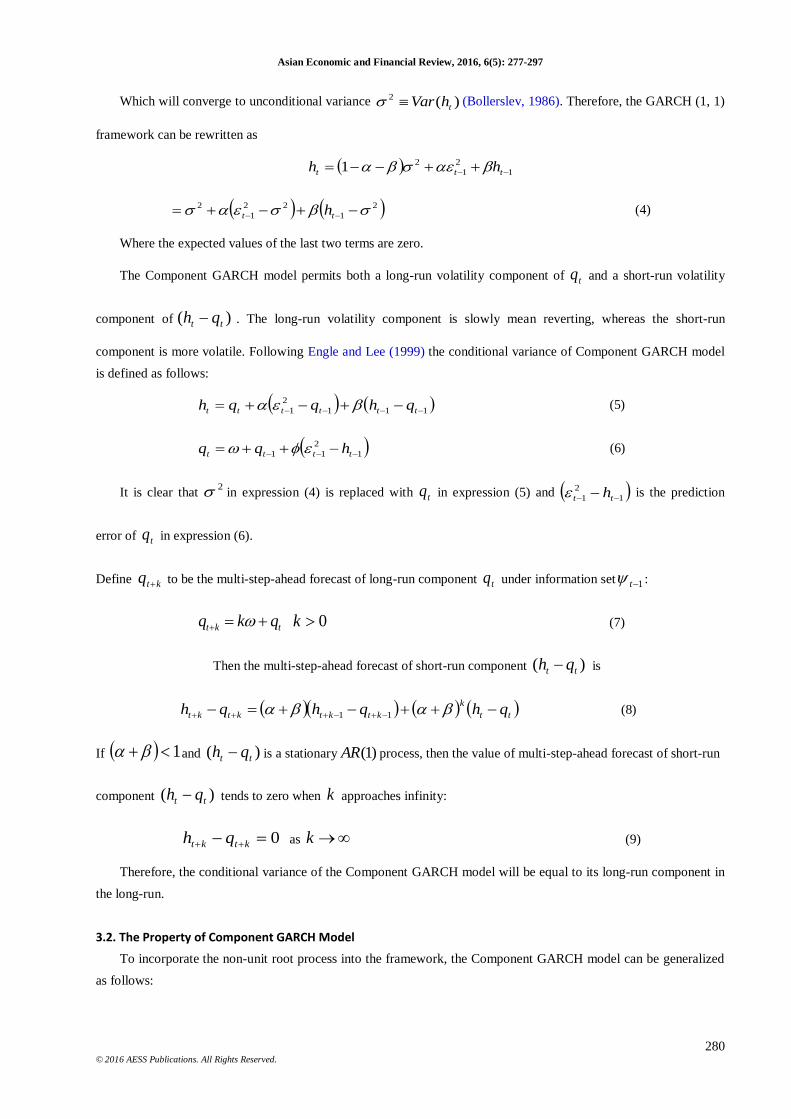
Which will converge to unconditional variance )(2

thVar (Bollerslev, 1986). Therefore, the GARCH (1, 1)

framework can be rewritten as

1

2

1

21 ttt hh

2

1

22

1

2 tt h (4)

Where the expected values of the last two terms are zero.

The Component GARCH model permits both a long-run volatility component of tq and a short-run volatility

component of )( tt qh . The long-run volatility component is slowly mean reverting, whereas the short-run

component is more volatile. Following Engle and Lee (1999) the conditional variance of Component GARCH model

is defined as follows:

111

2

1 tttttt qhqqh (5)

1

2

11 tttt hqq (6)

It is clear that 2 in expression (4) is replaced with tq in expression (5) and 1

2

1 tt h is the prediction

error of tq in expression (6).

Define ktq to be the multi-step-ahead forecast of long-run component tq under information set 1t :

tkt qkq 0k (7)

Then the multi-step-ahead forecast of short-run component )( tt qh is

tt

k

ktktktkt qhqhqh 11 (8)

If 1 and )( tt qh is a stationary )1(AR process, then the value of multi-step-ahead forecast of short-run

component )( tt qh tends to zero when k approaches infinity:

0 ktkt qh as k (9)

Therefore, the conditional variance of the Component GARCH model will be equal to its long-run component in

the long-run.

3.2. The Property of Component GARCH Model

To incorporate the non-unit root process into the framework, the Component GARCH model can be generalized

as follows:


281


111

2

1 tttttt qhqqh (10)

1

2

11 tttt hqq (11)

As long as , tq indicates that the conditional variance would exhibit the behavior of long-term

memory. The multi-step-ahead forecast of short- and long-run component under a more generalized Component

GARCH framework can be obtained as follows:

tt

k

ktkt qhqh (12)

t

kk

kt qq ]11[ (13)

The long-run volatility component will diminish faster than the short-run component when 1 , 1)(

, and )( . The conditional variance will converge to a constant when the long-run volatility component is

stationary:

1ktkt qh as k (14)

To examine the relationship between Component GARCH and GARCH models, substituting expression (11)

into expression (10) obtains

2

2

2

11 ttth

1 2t th h (15)

Thus, GARCH (2, 2) describes the conditional variance of Component GARCH framework. Distinguishing

short- and long-run volatility components enables Component GARCH framework to appropriately depict volatility

dynamics. The Component GARCH framework will be degenerated into GARCH (1, 1) model when α＝β＝0 or ρ＝

＝0 in expression (15). Therefore, the GARCH (1, 1) model only portraits plain dynamic relationships of

conditional variance through decomposition and component GARCH framework will portrait volatility dynamics

better than GARCH (1, 1) model.

Defining the prediction error tv tt h2

, expression (15) can be rewritten as

2

2

2

1

2 1 ttt

21 ttt vvv (16)

The squared innovation of Component GARCH framework follows an ARMA (2,2) process. We obtain the

following through expression (16):

2

2

2

1

2

1

2 1 tttt

21 ttt vvv (17)


282


Here it follows an ARIMA (1, 1, 2) process when ρ= l. The GARCH (1,1) model with α＝β＝0 could be

characterized by an ARIMA (0,1,1) process. Analogous to expressions (5) and (6), the previous expressions can be

obtained:

11

2

1

2

1 tttttt vvqq (18)

11 ttt vqq (19)

The maximum likelihood method is used to estimate the parameters of the variance process due to the

heterogeneity of error terms. The GARCH process is a covariance-stationary process if and only if the sum of its

dynamic parameters is less than one (Bollerslev, 1986). Under Component GARCH framework, the conditions of

stationary implies

11 (20)

The stationary conditions will achieve when ρ<1 and <1. If both short- and long-run volatility

components are covariance-stationary, the conditional variance also is covariance-stationary.

3.3. Volatility Persistency Test and Explanation

If the long-run component of conditional variance exhibits a unit-root process, i.e., an IGARCH (2, 2) the impact

of innovations on volatility will exhibit a persistent effect (Engle and Bollerslev, 1986). Therefore, we need to

explore the impact effect of volatility under Component GARCH framework. The following comparative statics can

be obtained from expressions (10) and (11):

2

1ttq (21)

2

1ttt qh (22)

Therefore, and α portrait the effects of unexpected shocks from short and long-run components of conditional

variance, respectively. The multi-period-ahead effects of a past innovation on short and long-run volatility

components are

k

tt

k

tkt qq

2

1

2

1 (23)

k

ttt

k

tktkt qhqh

2

1

2

1 (24)

The impact effect on volatility components will slowly decay when 1>ρ> . If 1 , the

impact effect on short-run volatility components will gradually vanish. However, the impact effect on long-run

volatility components will persist:

2

1

2

1 tttkt qq (25)

Under the Component GARCH framework, the Lagrange-multiplier and likelihood ratio tests can be used to test

the persistence of volatility.


283


3.4. Non-Negativity of Conditional Variance under Component GARCH Framework

To explore the non-negativity of conditional variance under the Component GARCH framework, substituting

expression (10) into expression (11) obtains

1

2

11 tttt hqh (26)

In which th follows time-varying GARCH (1, 1) process. If 1>ρ> >0 , β> >0, α>0, 0 , >0, and

>0, the conditional variance th maintains its non-negativity, so does the long-run volatility component tq .

Substituting expression (10) into expression (11) tq can be simplified to GARCH (2, 2) process in terms of past

squared innovations:

1

2

2

2

11 tttt qq 2 tq (27)

Under the Component GARCH framework, the non-negativity of long-run volatility component will be achieved

when 1>ρ> >0, β> >0, α>0, 0 , >0, and >0 (Nelson and Cao, 1992).

4. EMPIRICAL ANALYSIS

We explore the interactions between equity and exchange markets for Taiwan and Japan based on the

econometric models presented above. The main purpose here is to examine the goodness of fit of the Component

GARCH-M models for our data. Meanwhile, we will test the equity and foreign exchange risk impacts on the

expected returns of equity market. Firstly, we briefly describe the characteristics of the data. Secondly, we present the

results of unit root tests, serial correlation tests and ARCH effect tests on our data. Thirdly, the empirical model is

established. Finally, the empirical results of the Component GARCH-M models are presented.

4.1. Data Characteristics

We collected data for Taiwan’s weighted equity index and daily exchange rate data as well as for the Japan

Nikkei 225 equity index and daily exchange rate data. All data are daily close price and extracted from the

Datastream database. The sample period is from January 1, 1992 to December 31, 2011. Before the year 2000, in

Taiwan Saturdays were also trading days, meaning a total of six trading days per week; however, equity and

exchange markets in Japan are closed on Saturdays. To match the data, we deleted Saturday’s trading data in Taiwan

before 2000. In general, investors focus more on asset returns than on prices. From the viewpoints of econometrics,

the price series are not stationary. Hence, it is necessary to transform the price series into returns series. Traditionally,

we can achieve this by taking logarithmic and making first difference for the consecutive prices, i.e; Ri,t = (ln Pi,t –

lnPi,t-1). Where Ri,t denotes the return at the period t for the i-th country; and Pi,t is the closing price at the t day for the

i-th country. As for the foreign exchange market, the same method is applied for the closing price of exchange rates,

letting ri,t = (ln pi,t – ln pi, t-1). We distinguish the data of foreign exchange markets from equity markets with lower

case letters. Other than this, the definitions of variables are similar to the equity markets.

We summarize in Table 1 the basic statistics of the raw data for equity and foreign exchange markets in Taiwan

and Japan. Returns data for equity markets and foreign exchange markets in Taiwan and Japan also are outlined in

Table 2. In Table 1, both Taiwanese equity and foreign exchange markets display positive skewness. However, both

Japanese equity and foreign exchange markets are


284


Table-1. Summary statistics for equity prices and foreign exchange rates in Taiwanese and Japanese

markets

Equity Market Foreign Exchange Market

Taiwan Japan Taiwan Japan

Mean 6322.983 15181.33 30.783 112.638

Std dev 1528.443 3906.092 3.2186 11.261 Max 10202.200 23801.000 35.165 147.210

Min 3135.560 7054.980 24.507 80.620

Skewness 0.265 - 0.179 0.497 - 0.065

Kurtosis 2.634 1.894 1.723 3.016 Jarque-Bera 141.353*** 249.195*** 500.511*** 143.403***

)24(Q 71,324.000*** 72,044.000*** 74,104.000 *** 70,112.000*** Note: *** represents significant at 1% level.

Table-2. Rate of returns of equity prices and foreign exchange rates for Taiwanese and Japanese markets


Taiwan Japan Taiwan Japan Mean 0.005 - 0.008 0.002 - 0.003 Std dev 0.673 0.679 0.114 0.311

Max 2.833 5.748 1.470 2.786 Min - 3.029 - 5.260 - 1.165 - 2.773

Skewness - 0.112 0.108 1.295 - 0.419

Kurtosis 4.955 8.057 32.284 8.993 Jarque-Bera 768.037*** 4724.693*** 165184.600*** 7206.899***

)24(Q 74.124*** 31.825*** 308.812*** 38.421*** )24(2Q 532.810*** 460.115*** 984.227*** 794.134***

794.134***

Note: *** represents significant at 1% level.

Negatively skewed. Meanwhile, the Jarque-Bera statistics show that the data are not normally distributed.

Finally, autocorrelation tests (Q(24)) also reject the data being white noise. This shows that it is important to take the

first difference for stationarity.

We display the summary statistics for returns in Table 2. For our sample period, the returns for equity and

foreign exchange markets in Taiwan are positive. However, they are both negative for equity and foreign exchange

markets in Japan. As for skewness, the Taiwanese exchange market and Japanese equity market appear to be positive

skewed and other markets are negatively skewed. For the fourth moments (kurtosis) of the series, we find equity

markets and foreign exchange markets for these two countries to be more than 3. Namely, the data for equity and

exchange markets possesses fat tails. From Table 2, the data do not appear to be normally distributed from the J-B

statistics.

4.2. Unit Root, Serial-Correlation and ARCH Effect Tests

The early and pioneering work on testing for a unit root in a time series was done by Dickey and Fuller (DF).

Subsequently, Phillips and Perron (PP) developed a more comprehensive theory on the unit root non-stationarity. The

tests are similar to the augmented Dickey-Fuller (ADF) tests, but they incorporate an automatic correction to the DF

procedure to allow for auto-correlated residuals.

If we find that the data does possess a unit root, it means that the series is not stationary. One can use first order

difference to remedy the stationarity. After taking first order difference and changing the time series into a stationary

one, it is said to be integrated to the order of one, i.e., denoted I (1). In Tables 3, 4 and 5, we present the results for the

unit root test using the ADF test and the PP test, respectively. No matter which functional type is used for the original

data, namely the constant term and/or time trend, all of their test statistics are lower than the critical value. Therefore,


285


the price series and exchange rates are not stationary. However, after the first order differencing, all data follows a

stationary process based on conventional levels of significance.

We further test for series correlation. It is conventional to fit the auto-regressive model for the return’s mean

equation. However, these models have to satisfy no serial correlation for the residual terms and follow white noise.

For this purpose, we introduce Ljung-Box Q statistics developed by Ljung and Box. Meanwhile, the index of AIC

and SBC are incorporated for the selection of appropriate lag periods. All of the results are presented in Tables 6 to 8.

Basically, the optimal number of lag terms in the conditional mean equation is determined by the likelihood ratio test,

the results show that optimal lag length for the Taiwanese stock market is 4. And for the Taiwanese foreign exchange

market, Japanese stock and foreign exchange market, the optimal lag lengths are 2, based on the values of AIC/BIC

(Table 6, 7 and 8) under Ljumg–Box Q test.

Table-3. Unit root testing results of ADF and PP tests

Drift and Trend Drift W/o Drift and Trend

ADF

Taiwan Equity (5) -1.815 -1.982 -1.521

Japan Equity (3) -2.410 -1.201 -1.082

Tw Exch. Rate (3) -1.924 -0.801 -1.411

J. Exch. Rate (3) -2.201 -2.101 -0.358

PP

Taiwan Equity (5) -1.945 -1.982 -1.952

Japan Equity (3) -2.582 -1.701 -1.705

Tw Exch. Rate (3) -2.105 -0.902 -1.421

J. Exch. Rate (3) -2.055 -2.123 -2.215 Note: The number of lag periods is in parenthesis.

Table-4. The ADF and PP test results for logarithm of equity prices and exchange rates

Drift and Trend Drift W/o Drift and Trend

ADF

Taiwan Equity (5) -1.852 -2.145 -1.576

Japan Equity (3) -1.812 -0.464 -1.831

Two Exch. Rate (3) -1.802 -0.785 -1.412

J. Exch. Rate (3) -2.101 -2.012 -0.711

PP

Taiwan Equity (5) -1.953 -1.988 -1.648

Japan Equity (3) -2.301 -1.384 -1.925

Tw Exch. Rate (3) -2.162 -0.991 -1.546

J. Exch. Rate (3) -2.114 -1.041 -0.615 Note: The number of lag periods is in parenthesis

Table-5. ADF and PP tests results for the equity returns and the rate of returns of exchange rates

Drift and Trend Drift w/o Drift and Trend

ADF

Taiwan Equity (5) -25.815*** -25.810*** -25.161 ***

Japan Equity (3) -34.112 *** -34.152 *** -34.168***

Tw Exch. Rate (3) -25.710 *** -25.812 *** -25.144 ***

J. Exch. Rate (3) -32.452 *** -32.115 *** -33.699 ***

PP

Taiwan Equity (5) -55.112 *** -55.912 *** -54.612***

Japan Equity (3) -58.143 *** -58.321 *** -58.415 ***

Tw Exch. Rate (3) -69.112 *** -69.665 *** -69.713 ***

J. Exch. Rate (3) -57.623 *** -57.182*** -57.145 *** Note: *** represents significant at 1% level. The number of lag periods is in parenthesis.


286


Table-6. The optimal number of lag periods for equity markets

No

Taiwan Equity Japan Equity

AIC BIC AIC BIC

1 -169.596 -155.022 -1537.785 -1387.723

2 -170.762 -149.152 -1541.433*** -1388.335***

3 -169.863 -149.127 -1539.598 -1377.464

4 -175.868*** -148.188*** -1539.598 -1377.464

5 -174.195 -141.479 -1536.243 -1362.029

6 -172.027 -134.274 -1535.987 -1355.747


Table-7. Optimal number of lag periods for foreign exchange markets

Tw Exch. Rate J. Exch. Rate

AIC BIC AIC BIC

1 -9790.187 -9968.056 -5923.128 -5850.999

2 -9800.945*** -9872.780*** -5924.317*** -5843.152***

3 -9799.024 -9864.823 -5919.631 -5835.430

4 -9803.647 -9863.410 -5918.182 -5827.956

5 -9849.565 9903.288 -5916.361 -5828.090

6 -9848.139 -9895.831 -5916.260 -5813.953 Note: *** represents significant at 1% level.

Table-8. Residual tests of conditional mean equations for Taiwanese and Japanese equity and foreign

exchange markets


Taiwan Japan Taiwan Japan

Q(8) 1.832 2.512 2.657 3.612

Q(16) 15.012 10.682 13.778 13.672

Q(24) 21.116 25.195 24.621 23.118 2Q (8) 403.665*** 173.812*** 426.334*** 82.512***

2Q (16) 603.182*** 255.812*** 631.578*** 109.612***

2Q (24) 800.565*** 324.417*** 840.415*** 198.201***

Note: *** represents significant at 1%.

Finally, we show the results for ARCH effect. We perform the ARCH-LM test to determine whether an ARCH-

effect is present in the residuals of an estimated model, such as AR (p). We gather the AR (p)’s residuals, square the

residuals, and then regress them on their own lags to test for ARCH to the order of p. We can obtain R2 from this

regression. The test statistics is defined as TR2 from regression where T is the total number of observations, and is

distributed as a chi-squared distribution with the p degree of freedom. We describe these results in Table 9. It is clear

that these return series exhibit ARCH effects. Hence, it is appropriate to fit a GARCH model for further analysis.

Table-9. ARCH-LM tests of squared residuals of conditional mean equations for Taiwanese and

Japanese equity and foreign exchange markets


Lag Taiwan Japan Taiwan Japan

1 631.522*** 652.471*** 391.885*** 293.645***

2 661.801*** 640.471*** 392.732*** 305.852***

3 668.150*** 665.114*** 516.551*** 307.152***

4 690.150*** 675.114*** 625.401*** 310.402***

5 682.11*** 674.801*** 630.712*** 310.614***



287


4.3. Model Setups for Empirical Study

To understand the interactions of transitory and permanent risks on equity and foreign exchange markets, the

variable of return volatility is incorporated as a regressor into the conditional mean equation. The process can provide

the Information about risk premium in the short- and long-run situation. To build up various Component GARCH-M

models, we first define the relevant variables and parameters, and then construct the univariate Component GARCH-

M models to conduct our empirical analyses.

The relevant variables and parameters for various univariate Component GARCH-M models are defined as

follows:

RS and RE represent the Taiwanese equity and foreign exchange markets, respectively;

RS

ty and RE

ty represent the rate of returns of the Taiwanese equity and foreign exchange markets in period t,

respectively;

RS

t and RE

t represent the innovations of the Taiwanese equity and foreign exchange markets in period t,

respectively;

RS

th and RE

th represent the conditional variance of the rate of returns of the Taiwanese equity and foreign exchange

markets in period t, respectively;

RS

tq and RE

tq represent long-run volatility component of the Taiwanese equity and foreign exchange markets in

period t, respectively;

RS

ts and RE

ts represent short-run volatility component of the Taiwanese equity and foreign exchange markets in

period t, respectively, where ttt qhs ;

212121 ,,,,,,,,,,,, dddccc and 2 are relevant parameters to be estimated in various univariate

Component GARCH-M models.

The corresponding variables and parameters for the Japanese equity and foreign exchange markets are similarly

defined with RS and RE replaced by JS and JE respectively.

There are three Component GARCH-M models considered in this study. The first Component is the GARCH-M

model which is constructed to investigate the impact of endogenous equity volatility and exogenous foreign exchange

volatility on the rate of returns in equity markets and also to explore the effects of the short and long-run volatility

components on both Taiwanese and Japanese equity markets. Cases 1 and 2 characterize the corresponding

conditional mean and variance equations for Taiwanese and Japanese equity markets examined in the first

Component GARCH-M model:

CASE 1: Impact of endogenous equity volatility

4

1

0

k

RS

t

RS

t

RSRS

kt

RS

k

RSRS

t hcyaay

RS

t

RS

t

RSRS

t

RS

t

RSRS

t

RS

t qhqqh 111

2

1


288


RS

t

RS

t

RSRS

t

RSRSRS

t hqq 1

2

11

2

1

0

k

JS

t

JS

t

JSJS

kt

JS

k

JSJS

t hcyaay

JS

t

JS

t

JSJS

t

JS

t

JSJS

t

JS

t qhqqh 111

2

1

JS

t

JS

t

JSJS

t

JSJSJS

t hqq 1

2

11 (28)

CASE 2: Impact of exogenous foreign exchange volatility

4

1

0

k

RS

t

RE

t

RERS

kt

RS

k

RSRS

t hcyaay

RS

t

RS

t

RSRS

t

RS

t

RSRS

t

RS

t qhqqh 111

2

1

RS

t

RS

t

RSRS

t

RSRSRS

t hqq 1

2

11

2

1

0

k

JS

t

JE

t

JEJS

kt

JS

k

JSJS

t hcyaay

JS

t

JS

t

JSJS

t

JS

t

JSJS

t

JS

t qhqqh 111

2

1

JS

t

JS

t

JSJS

t

JSJSJS

t hqq 1

2

11 (29)

The second Component GARCH-M model is constructed to investigate the impacts of the short- and long-run

volatility components of endogenous equity volatility and exogenous foreign exchange volatility on returns of equity

markets and to explore the effects of the short and long-run volatility components on equity markets. Cases 3 and 4

characterize the corresponding conditional mean and variance equations in the second Component GARCH-M model:

CASE 3: Impact of the short- and long-run volatility components of endogenous equity volatility

4

1

210

k

RS

t

RS

t

RSRS

t

RSRS

kt

RS

k

RSRS

t scqcyaay

RS

t

RS

t

RSRS

t

RS

t

RSRS

t

RS

t qhqqh 111

2

1

RS

t

RS

t

RSRS

t

RSRSRS

t hqq 1

2

11

2

1

210

k

JS

t

JS

t

JSJS

t

JSJS

kt

JS

k

JSJS

t scqcyaay

JS

t

JS

t

JSJS

t

JS

t

JSJS

t

JS

t qhqqh 111

2

1

JS

t

JS

t

JSJS

t

JSJSJS

t hqq 1

2

11 (30)

CASE 4: Impact of the short- and long-run volatility components of exogenous foreign exchange volatility


289


4

1

210

k

RS

t

RE

t

RERE

t

RERS

kt

RS

k

RSRS

t scqcyaay

RS

t

RS

t

RSRS

t

RS

t

RSRS

t

RS

t qhqqh 111

2

1

RS

t

RS

t

RSRS

t

RSRSRS

t hqq 1

2

11

2

1

210

k

JS

t

JE

t

JEJE

t

JEJS

kt

JS

k

JSJS

t scqcyaay

JS

t

JS

t

JSJS

t

JS

t

JSJS

t

JS

t qhqqh 111

2

1

JS

t

JS

t

JSJS

t

JSJSJS

t hqq 1

2

11 (31)

The third Component GARCH-M model is constructed to investigate the impact of foreign exchange volatility

from the previous period and the short- and long-run volatility components of foreign exchange volatility from the

previous period on returns of equity markets and to explore the effects of the short- and long-run volatility component

on equity markets. Cases 5 and 6 characterize the corresponding conditional mean and variance equations in the third

Component GARCH-M model:

Case 5: Impact of exogenous foreign exchange volatility in the previous period

4

1

0

k

RS

t

RS

kt

RS

k

RSRS

t yaay

RE

t

RERS

t

RS

t

RSRS

t

RS

t

RSRS

t

RS

t hdqhqqh 1111

2

1

RS

t

RS

t

RSRS

t

RSRSRS

t hqq 1

2

11

2

1

0

k

JS

t

JS

kt

JS

k

JSJS

t yaay

JE

t

JEJS

t

JS

t

JSJS

t

JS

t

JSJS

t

JS

t hdqhqqh 1111

2

1

JS

t

JS

t

JSJS

t

JSJSJS

t hqq 1

2

11 (32)

Case 6: Impact of the short- and long-run volatility components of exogenous foreign exchange volatility in the

previous period

4

1

0

k

RS

t

RS

kt

RS

k

RSRS

t yaay

RE

t

RERE

t

RERS

t

RS

t

RSRS

t

RS

t

RSRS

t

RS

t sdqdqhqqh 1211111

2

1

RS

t

RS

t

RSRS

t

RSRSRS

t hqq 1

2

11


290


2

1

0

k

JS

t

JS

kt

JS

k

JSJS

t yaay

JE

t

JEJE

t

JEJS

t

JS

t

JSJS

t

JS

t

JSJS

t

JS

t sdqdqhqqh 1211111

2

1

JS

t

JS

t

JSJS

t

JSJSJS

t hqq 1

2

11 (33)

4.4. Empirical Results

This article employs the BHHH algorithm to obtain the estimates of consistent estimators. Tables 10 to 15

present the estimated coefficients of conditional mean and variance equations from six cases of the three Component

GARCH-M models. It can be seen from Tables 10 to 15 that the restrictions of the coefficients (α>0, β> >0, >0

and α+β<ρ<1), are fully satisfied for all cases of the three Component GARCH-M models, indicating that all

Component GARCH-M models constructed in this study are economically meaningful.

The Ljung-Box test statistics in Tables 10 to 15 reveal that for the first and second order moments of the residual

series on Taiwanese and Japanese equity and foreign exchange markets, the distributions of these residual series are

neither auto-correlated nor hetroskedastic. These verify that all Component GARCH-M models constructed are

appropriate for our empirical analyses.

Tables 10 and 11 summarize the impacts of equity and foreign exchange volatility on returns of equity markets

and the effects of the short and long-run volatility components on both the Taiwanese and Japanese equity markets.

As indicated in Table 10, the Taiwanese equity market returns are significantly affected by lagged second and fourth

periods, implying that investors exhibit bias expectations or the information is not fully reflected. The Taiwanese

equity market may not be efficient in the sense that the investors cannot have more time to be fully adjusted when

some shocks or events occur, however current returns may be predicted by using past information. The significantly

positive coefficient RSc reveals that the Taiwanese equity market returns are also affected by the equity volatility.

The positive risk-return relation indicates a positive risk premium in the market.

The significantly positive coefficient RS of the conditional variance equation shows that the unexpected shock

of volatility will impact the fluctuations in the Taiwanese equity market. For the long-run volatility components, the

estimated coefficient RS is .957, which is significant and close to one, indicating persistency in the long-run

volatility components of the Taiwanese equity market. Finally, the significantly positive coefficient RS reveals that

the long-run volatility components of the Taiwanese equity market will fluctuate when unexpected shocks of

volatility arrive on the market.

Similar results are found in Table 10 for the Japanese equity market except for the insignificant coefficient JSc ,

which shows that there is no significant positive risk-return relationship in the Japanese equity market due to possible

biases in investor’s expectations (Fu et al., 2011).


291


Table-10. Impact of endogenous equity volatility: Case 1

Conditional Mean Equation Conditional Mean Equation

Taiwan Japan coefficient t-value coefficient t-value

RS

0a -0.001* -1.870 JS

0a

-0.012 -1.612 RS

1a 0.018 1.032 JS

1a -0.043* -1.835

RS

2a 0.062** 2.615 JS

2a -0.002 -0.114

RS

3a 0.007 0.483 JSc 5.143 1.773 RS

4a -0.053** -2.342 RSc 6.585** 2.855

Conditional Variance Equation Conditional Variance Equation


RS 0.052*** 3.502 JS 0.059*** 3.667 RS 0.284 1.214

JS 0.212 0.607 RS 0.001*** 7.084 JS 0.004*** 7.554 RS 0.961*** 140.003 JS 0.980*** 184.115

RS 0.083*** 12.115 JS 0.081*** 10.215

)24(Q 14.339 )24(Q 17.524 )24(2Q 21.492 )24(2Q 24.152

Note: *, ** and *** represents significant at 10%, 5% and 1% level, respectively.

Table-11. Impact of exogenous foreign exchange volatility: Case 2


Taiwan Japan

coefficient t-value coefficient t-value RS

0a 0.001 1.154 JS

0a

-0.001 -0.203

RS

1a 0.031 1.265 JS

1a -0.042 * -1.817

RS

2a 0.051 ** 2.634 JS

2a -0.002 -0.071

RS

3a 0.021 0.571 JEc 0.901 0.181

RS

4a -0.062 ** -2.241

REc 0.181 0.046


Taiwan Japan

coefficient t-value coefficient t-value RS 0.0113 0.824 JS 0.0512 *** 3.477

RS 0.831 *** 2.820 JS 0.285 0.867

RS 0.001 *** 3.815 JS 0.002 *** 7.555

RS 0.982*** 121.004 JS 0.981*** 200.116 RS 0.067 *** 4.262

JS 0.081 *** 9.943

)24(Q 17.446 )24(Q 18.343

)24(2Q 22.110 )24(2Q 21.470


We find very similar results in Table 11 except for the foreign exchange exposure. The insignificant REc and

JEc in Table 11 indicate that both the Taiwanese and Japanese equity market returns are not affected by their foreign

exchange exposure. This is somewhat surprising. One of the possible reasons is that the risk of foreign exchange rate

consists of short-term risk (accounting risk) and long-term risk (economic risk) (Chiang et al., 2000). Thus, the short-


292


and long-term effects will not be fully reflected if short- and long-term risks are not decomposed appropriately in the

models.

Table-12. Impact of the short- and long-run volatility components of endogenous equity volatility: Case 3


Taiwan Japan

coefficient t-value coefficient t-value

RS

0a -0.009* -1.982 JS

0a

-0.001* -1.846

RS

1a 0.021 0.993 JS

1a

-0.042** -2.016

RS

2a 0.043** 2.235 JS

2a

-0.021 -0.690

RS

3a 0.046* 1.928 JSc1

9.142*** 5.012

RS

4a -0.068*** -3.412 JSc2 2.415 1.542

RSc1 1.701 0.281

RSc2 29.112*** 2.995


Taiwan Japan


RS 0.0612 *** 3.401 JS 0.053*** 3.411

RS 0.547 1.412 JS 0.681 1.281

RS 0.0122 1.063 JS 0.001*** 7.532 RS 0.912 *** 101.703 JS 0.982 *** 199.336 RS 0.071 *** 11.813 JS 0.092 *** 11.333

)24(Q 18.336 )24(Q 19.221

)24(2Q 22.113 )24(2Q 20.778

Note: *, **and *** represents significant at 10%, 5% and 1% level, respectively.

Tables 12 and 13 summarize the impact of the short and long-run components of equity and foreign exchange

volatility on the rate of returns and the effects of the short and long-run volatility component of both the Taiwanese

and Japanese equity markets. We focus on exploring the impacts of the short- and long-run components of equity and

foreign exchange volatility on returns of both markets. These results are very similar to those shown in Tables 10 and

11. The insignificant RSc1 and significant

RSc2 in Table 12 indicate that there is significant positive risk-return

relation and risk premium in the short-term on the Taiwanese equity market; in the long-term, the equity risk is not

fully reflected, possibly because there is a trading price limit and investors and enterprises take advantage of financial

instruments to hedge their risks or there are more individual investors in Taiwanese equity market who are irrational,

or institutional investors are less risk adverse (Barber et al., 2009; Chuang and Susmel, 2011).

On the other hand, the significant JSc1 and insignificant

JSc2 indicate that there is significant positive risk-return

relation and risk premium only in the long-term on the Japanese equity market. The possible reason is that the

proportion of financial institutional investors is large enough that only in the long-term will the equity market

generate structural change and greater fluctuations, and hence require more risk premium.


293


Table-13. Impact of the short- and long-run volatility components of exogenous foreign exchange volatility: Case 4



RS

0a -0.003 -1.032 JS

0a

-0.001 -1.124

RS

1a 0.032 1.314 JS

1a -0.031 -1.613

RS

2a 0.058** 2.512 JS

2a -0.004 -0.171

RS

3a 0.021 0.665 JEc1 13.117 1.463

RS

4a -0.051** -2.245 JEc2 -32.812** -2.545

REc1 18.554 1.062

REc2 -8.912 -0.915


Taiwan Japan

coefficient t-value coefficient t-value RS 0.012 0.656 JS 0.055 *** 3.412

RS 0.837** 2.136 JS 0.241 0.889

RS 0.000156 *** 2.931 JS 0.002*** 8.247 RS 0.982 *** 96.298 JS 0.982*** 198.996

RS 0.061*** 2.723 JS 0.081 *** 9.994

)24(Q 18.493 )24(Q 18.562 )24(2Q 20.151 )24(2Q 21.403

Note: ** and *** represents significant at 5% and 1% level, respectively.

Table-14. Impact of exogenous foreign exchange volatility in previous period: Case 5


Taiwan Japan

coefficient t-value coefficient t-value RS

0a 0.0013 1.381 JS

0a -0.001 -0.142

RS

1a 0.0211 1.422 JS

1a -0.031 -1.273

RS

2a 0.0521 *** 2.613 JS

2a -0.001 -0.083

RS

3a 0.0112 0.713

RS

4a -0.061 *** -2.282


Taiwan Japan


RS 0.004 0.898 JS 0.051 *** 3.241

RS 0.971*** 212.531 JS 0.283 0.813

RS 0.001*** 2.831 JS

0.002 *** 6.815

RS 0.991 *** 118.652 JS 0.874*** 190.335

RS 0.072 *** 8.714 JS 0.078 *** 8.815

RSd 0.020 *** 2.715 JSd -0.010 -0.734

)24(Q 17.141 )24(Q 19.114

)24(2Q 24.323 )24(2Q 21.497



294


Table-15. Impact of the short- and long-run volatility components of exogenous foreign exchange volatility in previous period: Case 6



RS

0a 0.001 1.413

JS

0a

-0.001 -0.272

RS

1a 0.031 1.246 JS

1a -0.051* -1.743

RS

2a 0.051** 2.644 JS

2a -0.002 -0.073

RS

3a 0.015 0.743

RS

4a -0.046** -2.415



RS 0.051 1.514

JS 0.051*** 3.243

RS 0.921*** 58.342 JS 0.287 0.816

RS 0.001*** 3.489 JS 0.001*** 7.876

RS 0.993*** 126.314 JS 0.981*** 185.493

RS 0.018 0.725 JS 0.081*** 9.999

RSd1 -0.271*** -3.414

JSd1 -0.010 -0.813

RSd2 0.081** 2.164 JSd 2

-0.004 -0.064

)24(Q 17.334 )24(Q 19.114

)24(2Q 24.816 )24(2Q 20.412


However, in the short run, the risk-return tradeoff in Japanese equity market may be caused by the bias

expectations of investors, or investors simply do not react to the new information quickly (Tai, 1999; Chiang and

Yang, 2003; Lin et al., 2009). The impacts of the short- and long-run components of foreign exchange volatility on

returns of both markets are reported in Table 13. As shown in Table 13, the insignificant REc1 and

REc2 indicate that

returns of the Taiwanese equity market are not affected by its foreign exchange exposure in either the short- and long-

run, possibly since investors and enterprises employ financial instruments to hedge their risks (Yau and Nieh,

2006;2009). The significantly negative JEc2 reveals that returns of the Japanese equity market decreases when foreign

exchange risks increase in the short-term. A possible reason is that a large proportion of financial institutional

investors possess a relatively high tolerance for risk taking in the short-term (Yau and Nieh, 2006;2009). Compared

with the results of case 2, the decomposition of the short and long-run components of foreign exchange volatility

facilitates reflecting the relative impact of foreign exchange exposure on returns of the Japanese equity market. This

result is supported by similar results from Pan et al. (2007) and Tai (2007).

Tables 14 and 15 report the results of the impacts of foreign exchange volatility in previous periods on

contemporaneous volatility. They also show the effects of the short and long-run volatility components on both equity

markets. We focus on investigating the impact of foreign exchange volatility in previous periods on contemporaneous

volatility. Other results are also similar to those found in Tables 10 and 11.

It can be seen from Tables 14 and 15 that the contemporaneous volatility will be significantly affected by the

short and long-run foreign exchange exposure in previous periods of the Taiwanese equity market, whereas the


295


contemporaneous volatility will not be affected by the short and long-run foreign exchange exposure in previous

periods of the Japanese equity market. The lagged response of foreign exchange exposure in previous periods on the

volatility of the Taiwanese equity market possibly reflects relatively greater foreign exchange rate risk for the large

trading volume of imports and exports that characterizes Taiwan’s economy (Wu, 1997; Yau and Nieh, 2006;2009;

Liu and Tu, 2012). This also confirms that there exists a cross-volatility spillover effect on the Taiwanese equity

market, including the short-term accounting and the long-term economic risks. Moreover, the insignificant response

of lagged foreign exchange exposure on the Japanese equity market possibly demonstrates that the Japanese economy

relies more on domestic demand and thus has a lower degree of the risk of foreign exchange rate (Choi et al., 1998;

Homma et al., 2005; Yau and Nieh, 2006;2009).

5. CONCLUSIONS

Recognizing the rising interest of financial econometrics on the investigation of the correlation between returns

in equity markets and the foreign exchange rates on foreign currency markets, we employed the bivariate Component

GARCH-M model. The analysis was based on Taiwan and Japan weighted equity index and exchange rate to analyze

the risk premium for both Taiwanese and Japanese equity markets. We further explore the permanent and transitory

effects of the short and long-run volatility components on both equity markets, and thus verify the effectiveness of the

model.

We find that through decomposing the time series effects of volatility into short and long-run components, the

conditional covariance trend (long-run) and transitory (short-run) components can be studied separately with a clear

improvement in the model’s performance due to its richer dynamics that makes it easier to jointly obtain the long and

short-term market returns.

For the returns of both Taiwanese and Japanese equity markets, the empirical results are significantly affected by

lagged periods, implying that both markets may not be fully efficient in the sense that the investors do not react

quickly to shocks or new events. Thus, returns are likely to be predicted by using past information and the unexpected

shock of volatility might in general influence fluctuations in both equity markets. In addition, persistency on long-run

volatility components from both markets was also found.

The positive risk-return relation indicates that there is risk premium in the Taiwanese equity market. On the other

hand, there is no significant positive risk-return relation in the Japanese equity market if the impacts from the short

and long-run volatility components are not decomposed.

Taking into account the short and long-run volatility components, the Taiwanese equity market exhibits positive

risk-return relation and risk premium only in the short-run. In the long-run, the equity risk is not fully reflected

possibly because there is a trading price limit and investors and enterprises take advantage of financial instruments to

hedge their risks. Furthermore, there are more individual investors in Taiwan equity market who are irrational or

institutional investors who are less risk adverse. On the other hand, the Japanese equity market exhibits positive risk-

return relation and risk premium only in the long-run, implying that the large proportion of financial institutional

investors may generate structural change and greater fluctuations, and hence require more risk premium in the long-

run. However, in the short-run, the risk-return tradeoff in the Japanese equity market may be caused by the bias

expectations in investors, or because they simply do not react quickly to new information.

The impact from short and long-run components of the foreign exchange volatility on returns from both markets

indicate that returns of the Taiwanese equity market are not influenced by its own foreign exchange exposure in either

the short or long-run. Possibly because investors and enterprises employ financial instruments to hedge their risks or

there are more individual investors in the Taiwanese equity market who are irrational. Or in other cases, institutional

investors may be less risk adverse. However, returns in the Japanese equity market decreases when the foreign


296


exchange risk in the short-run increases. Possibly since large proportions of financial institutional investors possess

relatively high tolerance on risk taking in the short-run or as the expected volatility risk rises. This might lead the

market uncertainty to increase, and the rational investors (speculators) might need incremental risk premium to

induce them to arbitrage away the mispricing. The decomposition of the short and long-run components from foreign

exchange volatility better detects the relative impact of foreign exchange exposure on returns of the Japanese equity

market.

Finally, the contemporaneous volatility is significantly affected by the short and long-run foreign exchange

exposure in previous periods of the Taiwanese equity market. The difference in characteristics of Taiwan and Japan’s

economic model may play a part in their respective exchange rate risk. While Taiwan’s exports account for roughly

60% of its GDP, Japan can potentially weather fluctuations in exchange rates by relying on domestic consumption

since its ratio of domestic consumption as a percentage of its GDP is above 55%.

REFERENCES

Barber, B.M.Y.T., Y.J.L. Lee and T. Odean, 2009. Just how much do individual investors lose by trading? Review of Financial

Study, 22(2): 609-632.

Bollerslev, T., 1986. Generalized autoregressive conditional heteroskedasticity. Journal of Econometrics, 31(3): 307-327.

Chiang, T.C. and S.Y. Yang, 2003. Foreign exchange risk premiums and time-varying equity market risks. International Journal of

Risk Assessment and Management, 4(4): 310-331.

Chiang, T.C., S.Y. Yang and T.S. Wang, 2000. Stock return and exchange rate risk: Evidence from Asian stock markets based on a

bivariate GARCH model. International Journal of Business, 5(2): 97-117.

Choi, J.J., T. Hiraki and N. Takezawa, 1998. Is foreign exchange risk priced in the Janpanese stock market? Journal of Financial

and Quantitative Analysis, 33(3): 361-381.

Christoffersen, P.F., K. Jacobs and Y. Wang, 2008. Option valuation with long-run and short-run volatility components. Journal of

Financial Economics, 90(3): 272-297.

Chuang, W.I. and R. Susmel, 2011. Who is the more overconfident trader? Individual versus institutional investors. Journal of

Banking and Finance, 35(7): 1622-1644.

Engle, R.F., 1982. Autoregressive conditional heteroskedasticity with estimates of the variance of UK inflation. Econometrica,

50(4): 987-1007.

Engle, R.F. and T. Bollerslev, 1986. Modelling the persistence of conditional variances. Econometric Reviews, 5(1): 1-50.

Engle, R.F. and G.G.H. Lee, 1999. A long-run and short-run component model of stock return volatilityI in cointegration,

causality, and forecasting. Eds., by Engle and White. Co-integration, Causality and Forecasting. Oxford: Oxford

University Press. pp: 475-497.

Engle, R.F., D.M. Lilien and R.P. Robins, 1987. Estimating time-varying risk premia in the term structure: The ARCH-M model.

Econometrica, 55(2): 391-407.

Fu, T.Y., M.J. Holmes and F.S. Choi, 2011. Volatility transmission and asymmetric linkages between the stock and foreign

exchange markets: A sector analysis. Studies in Economics and Finance, 28(1): 36-50.

Homma, T., Y. Tsutsui and U. Benzion, 2005. Exchange rate and stock prices in Japan. Applied Financial Economics, 15(7): 469-

478.

Lee, C.H., S. Lin, H. and Y.C. Liu, 2010. Volatility and trading activity: An application of the component- GARCH model.

Empirical Economics Letters, 9(2): 99-106.

Lee, G.J., 1999. Contemporary and long-run correlations: A covariance component model and studies on the S&P 500 cash and

futures markets, Journal of Futures Markets, 19(8): 877-894.


297


Lin, S.Y., H.M. Chuang and D. Shyu, 2009. Time-varying risk premia, heterogeneous investors and the dynamics of exchange rate

and stock returns. International Research Journal of Finance and Economics, 28: 120-133.

Liu, H.H. and T.T. Tu, 2012. Mean-reverting and asymmetric volatility switching properties of stock price index, exchange rate

and foreign capital in Taiwan. Asian Economic Journal, 25(4): 375-395.

Nelson, D.B. and C.Q. Cao, 1992. Inequality constraints in the univariate GARCH model. Journal of Business and Economic

Statistics, 10(2): 229–235.

Pan, M.S., R.C.W. Fok and Y.A. Liu, 2007. Dynamic linkages between exchange rates and stock prices: Evidence from East Asian

markets. International Review of Economics and Finance, 16: 503-520.

Tai, C.S., 1999. Time-varying risk premia in foreign exchange and equity markets: Evidence from Asia-pacific countries. Journal

of Multinational Financial Management, 9(3-4): 291-316.

Tai, C.S., 2007. Market integration and contagion: Evidence from Asian emerging stock and foreign exchange markets. Emerging

Markets Review, 8(4): 264-283.

Watanabe, T. and K. Harada, 2006. Effects of the bank of Japan's intervention on Yen/Dollar exchange rate volatility. Journal of

the Japanese and International Economies, 20(1): 99-111.

Wu, J.L., 1997. Foreign exchange market efficiency and structural instability: Evidence from Taiwan. Journal of Macroeconomics,

19(3): 591-607.

Yau, H.Y. and C.C. Nieh, 2006;2009. Interrelationships among stock prices of Taiwan and Japan and NTD/ Yen exchange rate.

Journal of Asian Economics, 17(3): 535-552.

Yau, H.Y. and C.C. Nieh, 2009. Testing for cointegration with threshold effect between stock prices and exchange rates in Japan

and Taiwan. Japan and World Economics, 21(3): 292-300.

Views and opinions expressed in this article are the views and opinions of the authors, Asian Economic and Financial Review shall not be

responsible or answerable for any loss, damage or liability etc. caused in relation to/arising out of the use of the content.

A COMPARATIVE STUDY OF THE TAIWAN AND JAPAN EQUITY …5)-277-297.pdf · A COMPARATIVE STUDY OF THE...

Documents

Transcript of A COMPARATIVE STUDY OF THE TAIWAN AND JAPAN EQUITY …5)-277-297.pdf · A COMPARATIVE STUDY OF THE...