A Comparative Study of Pose Representation andDynamics Modelling for Online Motion Quality

Assessment

Lili Tao, Adeline Paiement, Dima Damen, Majid Mirmehdi, Sion Hannuna,Massimo Camplani, Tilo Burghardt, Ian Craddock

Faculty of EngineeringUniversity of Bristol

Bristol BS8 1UB

Corresponding Author: Majid Mirmehdiemail: majid@cs.bris.ac.uk

Tel: +441179545139Fax: +441179545209

Abstract

Quantitative assessment of the quality of motion is increasingly in demand byclinicians in healthcare and rehabilitation monitoring of patients. We study andcompare the performances of different pose representations and HMM models ofdynamics of movement for online quality assessment of human motion. In a gen-eral sense, our assessment framework builds a model of normal human motionfrom skeleton-based samples of healthy individuals. It encapsulates the dynam-ics of human body pose using robust manifold representation and a first-orderMarkovian assumption. We then assess deviations from it via a continuous onlinemeasure. We compare different feature representations, reduced dimensionalityspaces, and HMM models on motions typically tested in clinical settings, such asgait on stairs and flat surfaces, and transitions between sitting and standing. Ourdataset is manually labelled by a qualified physiotherapist. The continuous-stateHMM, combined with pose representation based on body-joints’ location, outper-forms standard discrete-state HMM approaches and other skeleton-based featuresin detecting gait abnormalities, as well as assessing deviations from the motionmodel on a frame-by-frame basis.

Keywords: Human Motion Quality, Human Motion Assessment,Continuous-State HMM Motion Analysis, Motion Abnormality Detection

Preprint submitted to Computer Vision and Image Understanding December 3, 2015

1. Introduction

Modelling and analysing human motion have been subject to extensive re-search in computer vision, in terms of feature extraction [1], action representation[2, 3], action recognition [4, 5], and abnormality detection [6]. While such worksmostly apply to the challenging tasks of motion and action detection and recog-nition, only a few manage to provide a quantitative assessment of human motionquality. Such assessment aims at quantifying the motion quality from a functionalpoint of view by assessing its deviation from an established model. This has poten-tial use in many scenarios, for example, in sport applications [7], and for physio-therapists and medics [8], who may, for example, estimate the normality of humanmovement, possibly relative to a specific age group, or to quantify the evolutionof their mobility during rehabilitation with respect to a personalized, preoperativemodel. Interestingly, physiotherapists assess human motion by visually observinga person’s ability to perform vital movements, such as walking on a flat surface,sitting down, and gait on stairs, by rating the deviation from a normal movementusing standard scores [9, 10]. These well established scores are subjective andare insufficient to effectively monitor patients on a regular basis, as they can onlybe used by well-trained specialists and thus require the patients to be evaluatedin clinical practices. Automated motion quality assessment can help in obtaininga more quantitatively accurate and temporal (inter-person and intra-person) com-parative measure. It would also be essential for continuous assessment outside ofa clinic, for example for use in the home for health and rehabilitation monitoring.

In addition to providing an overall score of ‘normality’, an online assessmentmeasure can provide an immediate estimation of what parts of the motion deviatefrom normal, towards a more detailed understanding of the quality of the mo-tion. The nature of online measures also enables assessing the motion before ithas completed, thus allowing to trigger alerts, such as fall prevention in cases ofunusually unstable gait.

This paper details and evaluates a method, first introduced in [11], for onlineestimation of the quality of movement from Kinect skeleton data, and presentsits application to clinic-related movement types. To enable such an online as-sessment, a few challenges have been dealt with: (1) motion-related features areextracted from skeleton data and compacted into a lower-dimensional space toproduce a simpler and more appropriate representation of pose, (2) a statisticalmodel of human motion, that encapsulates both the appearance and the dynamics

2

of the human motion, is learnt from training data of multiple individuals, suitablefor periodic and nonperiodic motions, (3) an online quantitative assessment ofmotion is obtained by reference to the learnt model, which evaluates deviations inboth appearance and dynamics on a frame-by-frame basis.

In [11], we proposed a framework in order to address these challenges, wherewe extracted 3D joint positions as a low-level feature, reduced their dimensional-ity while capturing their non-redundant information using a modified diffusionmaps manifold method (challenge 1 above), modelled human movement withrespect to a custom-designed statistical model (challenge 2), and evaluated themovement from an online measure based on the likelihood of the new observationto be described by such a model (challenge 3).

This article updates and expands the work in [11], providing more thoroughcomparative evaluations of its framework and a comprehensive assessment of itsindividual modules, with the following additions: (a) in order to both demonstratethe versatility of our framework and further evaluate it, we apply our method toa variety of movement types, both periodic and non-periodic. (b) We show thatthe statistical model we introduced in [11] is in fact a continuous-state HMM,and we put it in perspective with more conventional variations of general HMM-based models. In particular, we compare their respective suitability to the task ofcapturing the dynamics of movements. (c) We assess what is the optimal poserepresentation for our HMM-based model of dynamics. First, as well as the jointposition feature extracted from the skeleton data, we propose and compare againstadditional possible low-level skeletal features as some are more suitable for cer-tain HMM models and for describing certain motions. Second, we investigatethe optimum number of dimensions required in the manifold representations fordescribing the various low-level features. We also evaluate how the optimal poserepresentation varies with motion type. (d) We investigate whether the use of full-body information is beneficial for building pose representations, in particular formovements that are traditionally studied using partial-body information such asjoints in the analysis of gait. (e) We propose a new online measure for qualityassessment, and we compare it with the measure presented in [11].

Evaluation is performed on clinic-related motions of gait on stairs, walkingon a flat surface, and transitions between sitting and standing – actions that areparticularly relevant to the assessment of lower-extremity injuries. On the basisof testing on the dataset released in [11], a variety of common lower-extremity in-juries are included in the test sequences. The groundtruth is labelled by a qualifiedphysiotherapist.

Next, a review of the existing literature is provided in Section 2. Section 3

3

describes the framework for assessing the quality of a movement from skeletondata, introducing four variations of HMM techniques that are tested on our dataset.The experimental results are presented in Section 6, followed by a discussion andconclusion.

2. Related Work

To consider the state-of-the-art, we now review related works on robust featureextraction from skeleton data, building a model of human motion from trainingdata, and motion abnormality detection and quality of motion assessment, fromboth computer vision and clinical points of view.

2.1. Skeleton data from the Depth SensorsA large number of studies have attempted to efficiently extract features from

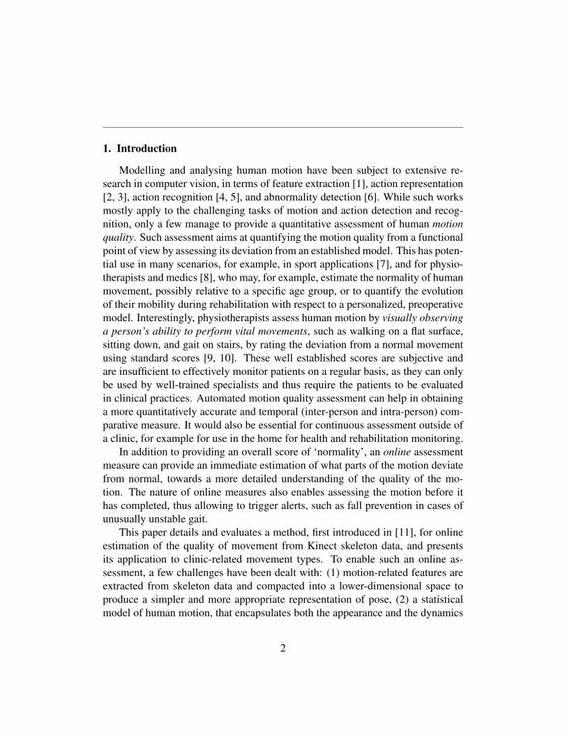
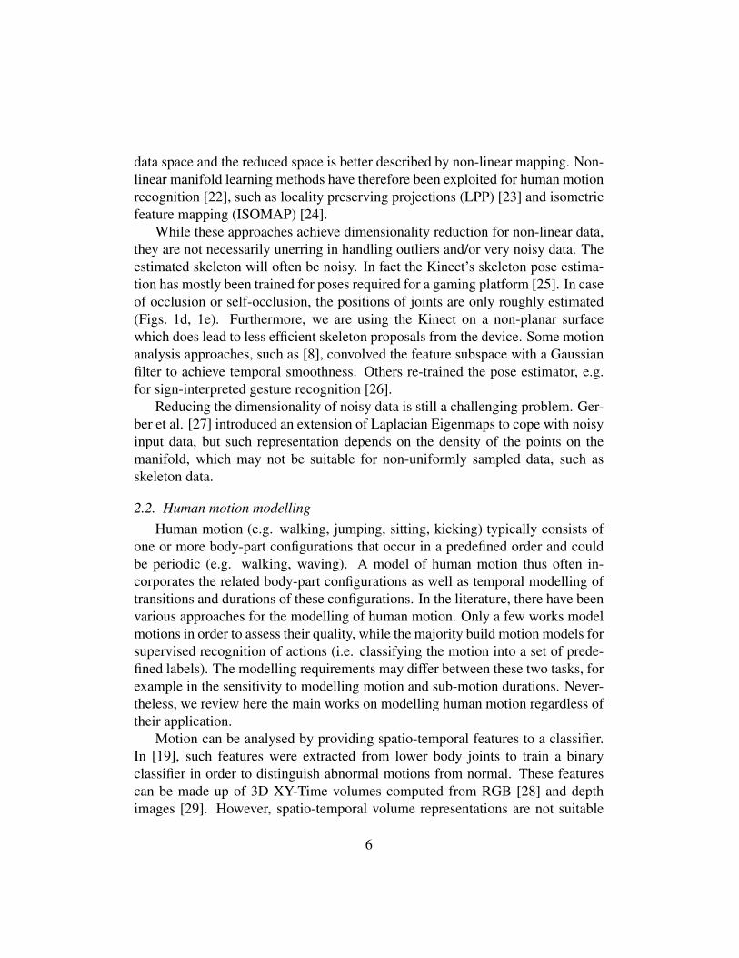
RGB images for analysing human actions, e.g. see [3], but RGB data is highlysensitive to view-point variations, human appearance, and lighting conditions. Re-cently, depth sensors have helped to overcome some of these limitations. Twocommercially available devices are the Microsoft Kinect and Asus Xmotion, forwhich the depth is computed from structured light1. These sensors have becomepopular for modelling and analysing human motion, for example in [12], Uddinet al. extracted features from depth silhouettes using Local Directional Patternsand applied Principal Component Analysis (PCA) to reduce the dimensionality oftheir data. More commonly, motion analysis works exploit skeleton informationderived from depth. Using random forests, 3D human skeletons are estimated ateach frame from depth data by the Microsoft Kinect SDK [13] (for 20 joints) or bythe OpenNI SDK [14] (for 15 joints). A human body pose can be well-representedas a stick figure made up of rigid segments connecting body joints. In this work,we use the OpenNI SDK to estimate skeleton data, as illustrated in Fig. 1. Wefocus next on methods that are based on skeleton features and refer the reader toa recent survey on non-skeleton features in [2].

Existing skeleton-based approaches have either used the full set of joints forgeneral action recognition [15, 16, 17, 18] or a subset chosen depending on thespecific action/application [19, 8]. In [19], only hips, knees, ankles and feet jointswere used for detecting abnormal events during stair descent. The method in [8]used feet joints along with the projection of hand and torso joints for evaluating

1Microsoft Kinect 2, released in 2014, uses time-of-flight technology

4

(a) (b) (c)

(d) (e)

Figure 1: RGB-D data and skeletons at bottom, middle, and top of the stairs ((a) to (c)), andexamples of noisy skeletons ((d) and (e)).

musculoskeletal disorders on patients who suffer from Parkinson’s Disease (PD).To avoid action-specific approaches, we use the full set of joints along with di-mensionality reduction techniques, explained next.

Robust Feature Extraction from Skeleton DataA variety of low-level features have been used to represent the skeleton data:

body joint locations [20], body joint velocities [17], body joint orientations [16],relative body joint positions [18], rigid segment angles [21] and transformations(rotations and translations) between various body segments [15]. Some of theseproposed features may be more suitable for describing certain motions than oth-ers, e.g. the relative position and orientation between head and foot may providesufficient description for the ‘sitting’ motion for some applications.

The high dimensionality of full-body skeleton data contains redundant infor-mation when modelling human motion, as will be demonstrated in Section 3.2.It is thus possible to employ dimensionality reduction methods to capture the in-trinsic body configuration of the input data. It is common to apply linear PCA fordimensionality reduction in appearance modelling, however, human motion repre-sented by skeleton data is highly non-linear and the mapping between the original

5

data space and the reduced space is better described by non-linear mapping. Non-linear manifold learning methods have therefore been exploited for human motionrecognition [22], such as locality preserving projections (LPP) [23] and isometricfeature mapping (ISOMAP) [24].

While these approaches achieve dimensionality reduction for non-linear data,they are not necessarily unerring in handling outliers and/or very noisy data. Theestimated skeleton will often be noisy. In fact the Kinect’s skeleton pose estima-tion has mostly been trained for poses required for a gaming platform [25]. In caseof occlusion or self-occlusion, the positions of joints are only roughly estimated(Figs. 1d, 1e). Furthermore, we are using the Kinect on a non-planar surfacewhich does lead to less efficient skeleton proposals from the device. Some motionanalysis approaches, such as [8], convolved the feature subspace with a Gaussianfilter to achieve temporal smoothness. Others re-trained the pose estimator, e.g.for sign-interpreted gesture recognition [26].

Reducing the dimensionality of noisy data is still a challenging problem. Ger-ber et al. [27] introduced an extension of Laplacian Eigenmaps to cope with noisyinput data, but such representation depends on the density of the points on themanifold, which may not be suitable for non-uniformly sampled data, such asskeleton data.

2.2. Human motion modellingHuman motion (e.g. walking, jumping, sitting, kicking) typically consists of

one or more body-part configurations that occur in a predefined order and couldbe periodic (e.g. walking, waving). A model of human motion thus often in-corporates the related body-part configurations as well as temporal modelling oftransitions and durations of these configurations. In the literature, there have beenvarious approaches for the modelling of human motion. Only a few works modelmotions in order to assess their quality, while the majority build motion models forsupervised recognition of actions (i.e. classifying the motion into a set of prede-fined labels). The modelling requirements may differ between these two tasks, forexample in the sensitivity to modelling motion and sub-motion durations. Never-theless, we review here the main works on modelling human motion regardless oftheir application.

Motion can be analysed by providing spatio-temporal features to a classifier.In [19], such features were extracted from lower body joints to train a binaryclassifier in order to distinguish abnormal motions from normal. These featurescan be made up of 3D XY-Time volumes computed from RGB [28] and depthimages [29]. However, spatio-temporal volume representations are not suitable

6

for online analysis as the motion analysis can only take place once the full motionsequence is observed.

Motion can also be seen as a sequence of body-part configurations. DynamicBayesian networks, such as Hidden Markov models (HMMs) and their variations,are the most popular generative models for sequential data and have been success-fully used as probabilistic models of human motion, e.g. human gait [30, 31, 16].In HMMs, each hidden state is associated with a collection of similar body posesand a transition model encapsulates sequences of body-part configurations. Themost common HMM model is one that uses a fixed number of discrete states,known as the classical HMM, along with a discrete observation model. This hasbeen used to recognise 10 basic actions in [16], and to classify motions betweennormal and abnormal in [12]. Continuous HMMs, which also use discrete statesbut continuous observation models such as a mixture of Gaussians, were used torecognise 22 actions in [31] and to distinguish normal from abnormal motionsin [32]. Particularly in [32], optical flow features, together with feet position andvelocity, were used to detect abnormalities during stairs descent from RGB data.The model uses 10 hidden states with full-covariance Gaussian mixture emissionsand random initialisation of the EM algorithm. A single extra state with high co-variance, low mixture proportion, and low transition probabilities were added forregularisation.

Apart from classical HMMs, extensions of HMMs introducing more flexiblemodels have been widely applied. A hierarchical HMM (HHMM) was used in[33] along with a time-varying transition probability. Three-level hierarchies wereimplemented representing composite actions, primitive actions and poses respec-tively. In [34], a factored-state HHMM was used to define each state as a hierarchyof two-levels for each action and tested on a dataset of 4 basic actions.

For periodic motions, a cyclic HMM was tried on 4 basic actions in [35].HMM variations that model state durations are frequently applied in activity recog-nition where temporal dependencies can be found. For example, Duong et al. [36]modelled the duration of each atomic action within an activity using a Coxian dis-tribution, and thus modelled the activity by an HMM with explicit state durations.To the best of our knowledge, HMM modelling of state duration has never beenapplied to the modelling of human motion.

Online motion modelsDepending on the application, the analysis can be either run offline incorporat-

ing data across the motion sequence, or processed online analysing an incomingframe before the entire motion is complete. Online motion models are important

7

for scenarios such as surveillance, healthcare, and gaming. Most HMM-basedmotion modelling approaches mentioned above require temporal segmentation,and therefore are restricted to offline processing. The work in [33] dealt with on-line gesture recognition using a hierarchical HMM. To achieve online recognition,the method extended the standard decoding algorithm to an online version usinga variable window [37], since the Viterbi algorithm cannot be directly applied toonline scenarios.

Nowozin and Shotton [38] developed an online human action recognition sys-tem by introducing action points for precise temporal anchoring of human actions.Recently, works based on incremental learning have been applied to human mo-tion analysis. In [39], an incremental covariance descriptor and on demand nearestneighbour classification were used for online gesture recognition. Instead of usingincremental features, the work in [40] proposes a general framework via nonpara-metric incremental learning for online action recognition which can be applied toany set of frame-by-frame feature descriptors.

2.3. Quality of motion assessmentWe define the quality of motion as a continuous measure of the ability of the

person to perform the motion when compared to a reference motion model. Sucha model represents the normal range of motions (we simply refer to normal motionin the rest of the article.) for the relevant population group, or it could be a person-alized model, and can be used to assess rehabilitation or pathological deteriorationin mobility of humans for healthcare purposes. For example, quantitatively assess-ing the ability to balance on one leg following a knee replacement surgery couldbe used to track a person’s rehabilitation. Similarly, Parkinson’s patients’ abilityto stand up from a sitting position deteriorates with time, and continuous assess-ment of this functionality is needed to evaluate the progress of the disease [8].The number of works targeting quality of motion are rare, with most attemptingto perform abnormality detection as binary classification. Thus, we first brieflyreview some abnormality detection methods, and then focus on the small numberof works on quantifying the degree of abnormality in human motion. We finishby presenting the current clinical approach for analysing motion quality.

2.3.1. Abnormality detectionAbnormality detection methods build a binary classifier to discriminate be-

tween normal and abnormal instances. Two main approaches exist, those thatassume prior knowledge of expected abnormalities, and those that do not. In thefirst approach, the work of [19] used two support vector machine (SVM) binary

8

classifiers that recognised normal and abnormal motions respectively, based onspace-time features. The approach was tested on stairs descent and ascent mo-tions, and it labelled normal and abnormal motions (e.g. fall or slip) from theclassifier with the strongest response. Similarly, the work of [12] trained twoHMMs on normal and abnormal gaits. Classification was also based on compar-ing the likelihood of the test sequence using both of these HMM models. No cleardefinition of ‘abnormal’ was provided in [12], and abnormalities encompassed awide range of anomalies.

Abnormal motions may be highly variant and difficult to define a priori. Mostabnormalities are rare and difficult to capture during training. The second ap-proach, where there is no prior knowledge of abnormalities, predicts them as vari-ations from the model of normal motion, built solely from regular/normal exam-ples. This approach thus aims to quantitatively estimate the dissimilarity from thenormal model - a kind of novelty detection. While this is a sensible compromise,the motion model needs to capture as much variation of normal motion examplesas possible to avoid high false negative rates.

In [41], hierarchical appearance and action models were built for normal move-ments to detect abnormalities from RGB silhouettes in a home environment. Forboth hierarchies, appearance and action, the intra-cluster distance within a nodewas used to set a threshold for abnormalities.

The work that is most closely related to ours is [32] which used a singleHMM for detecting abnormalities during stairs descent from RGB (only) data.The HMM was trained on sequences of normal ‘descending stairs’ motion, anda threshold on the likelihood was selected to detect abnormal sequences. Theirresults showed their system can successfully detect nearly all anomalous eventsfor data captured in a controlled laboratory environment, but is highly reliant onaccurate feet tracking.

2.3.2. Quality assessment of motionQuality assessment focuses on calculating a discrete or continuous score that

measures the match between a motion and a pre-trained model. Wang et al. [8]presented a method for quantitatively evaluating musculoskeletal disorders of pa-tients who suffer from PD. One motion cycle from the training data was selectedas a reference, and all other cycles were aligned to the reference for encodingthe most consistent motion pattern. The method was tested for walking, as wellas standing up, motion on PD and non-PD subjects. Results demonstrated thatthe method is able to quantify a clinical measurement which reflects a subject’smobility level. However, the specific features used (step size, arms and postural

9

swing levels, and stepping time) make it difficult to generalise to other motions.In a recent work on action assessment from RGB data, presented in [7], the

quality assessment was posed as a supervised non-linear regression problem. Themethod provided a feedback score on how one performs in sports actions, partic-ularly diving and figure skating, by comparing a test sequence with the labelledscores provided by coaches. Training a regression model required a relativelylarge number of labelled data points covering the spectrum of possible feedbackscores.

In [11], we proposed a continuous measure of motion quality, computed on-line, as the log-likelihood of a continuous-state HMM model. To the best of ourknowledge, [11] is the first and only work to address the problem of online qualityassessment.

3. Proposed Methodology

In this section, we describe our pipeline for assessing the quality of motionfrom skeleton data, as illustrated in Fig. 2. Skeleton data are first obtained fromthe OpenNI SDK [14]. Then, a low-level feature extraction stage (Section 3.1)determines a descriptor from the skeleton data. This is followed by a dimension-ality reduction step that is made less sensitive to noise and non-linear manifoldlearning (Section 3.2). In the reduced space, the significant and non-redundantaspects of the pose and the dynamics of the motion are expected to be preserved.A model of the motion is then learnt off-line from instances of ‘normal motion’(Section 3.3). The quality of movement is assessed by measuring the deviation ofa new observation from the learned model (Section 5).

This pipeline was first presented in our previous work [11] where only one pos-sible low-level skeleton feature and one possible motion model were discussed.Here, we introduce and compare different low-level features, and we assess ourmotion modelling method with respect to more traditional discrete HMM-basedmodels.

3.1. Skeleton data representationSkeleton data are view-invariant2 and depth information alleviates the effect

of human appearance differences and lighting variations. As a first step, we applyan average filter over a temporal window for each joint position independently

2Although the performance of the OpenNI SDK skeleton tracker suffers severely when thesubject is not facing the camera.

10

Figure 2: Proposed pipeline for movement quality assessment: the dashed lines denote a learningphase that is performed off-line to create the two models represented by the dashed rectangles.

in order to compensate for the high amount of noise typically found in OpenNIskeletons.

Given J joints, where J = 25 or J = 15 for skeletons from the MicrosoftKinect2 SDK or OpenNI SDK respectively, and a pose C = [c1, · · · , cJ ]T ∈R3J×1 comprising smoothed 3D positions ci in J , a normalised pose C = g(C)is computed to compensate for global translation and rotation of the view point,and for scaling due to varying heights of the subjects. The normalising functiong(�) could be Procrustes alignment or other alignment approaches depending onwhich feature is in use. Let F t be the low-level skeleton feature at time t. Usingfeatures that previously appeared in works such as [16, 17, 18, 20], we scrutinizefour possible alternative feature descriptors for normalised pose:

1. Joint Positions (JP): concatenate and vectorise 3D coordinates ci of all thejoints at time t, to give features F t = Ct.

2. Joint Velocities (JV): concatenate and vectorise the 3D velocities of all thejoints, to give features F t = Ct − Ct−1.

3. Pairwise Joint Distances (PJD): Given 3D positions of a normalised pose,we calculate a J × J Euclidean distance matrix between all pairs of jointswhere dij = ‖ci − cj‖. Since this is a symmetric matrix with zero en-tries along the diagonal, we obtain a J(J − 1)/2 feature vector F t =[d12, · · · , d1J , d23, · · · , d(J−1)J ]T . The pairwise joint distances give uniquecoordinate-free representation of the pose kinematics.

4. Pairwise Joint Angles (PJA): The Kinect skeleton of the human body con-sists of J−1 line segments connecting pairs of neighbouring joints. Assum-ing the segment ei connects two joints Ji and Ji+1, the Euler angle between

11

two segments is computed as ρij = arccos(eTi ·ej‖ei‖‖ej‖). Our feature vector F t

is a (J − 1)(J − 2)/2 vector that consists of all the Euler angles for allsegments, such that F t = [ρ12, · · · , ρ1(J−1), ρ23, · · · , ρ(J−2)(J−1)]T . Con-catenating all the Euler angles between any two body segments captures thefull 3D angles between body parts.

In the rest of this article, unless specified otherwise, these four feature descrip-tors are computed using all 25 or 20 body-joints from Kinect2 SDK or OpenNISDK, respectively, and so represent the whole skeleton.

3.2. Robust manifold learningAs previously noted, skeleton data is highly redundant for modelling motion

and does not represent its true complexity. To reduce the dimensionality of thelow-level feature Fi, we select a non-linear manifold learning method - diffusionmaps - which is a graph-based technique with quasi-isometric mapping Φ, fromoriginal higher space RN to a reduced low-dimensional diffusion space Rn, wheren� N . Given a training set F, where Fi ∈ F, the method is capable of recoveringthe underlying structure of a complex manifold, has robustness to noise, and isefficient to implement when compared to conventional non-linear dimensionalityreduction methods [42].

Building diffusion maps requires computing a weighted adjacency matrix Wwith the distances between neighbouring points weighted by a Gaussian kernelG:

wi,j = G (Fi, Fj) (1)

The optimal mapping Φ is obtained from the eigenvalues δ and the correspondingeigenvectors ϕ of the Laplace-Beltrami operator L [42],

Φ(Fi) 7→ [δ1ϕ1(Fi), · · · , δnϕn(Fi)]T , (2)

retaining the first n eigenvectors (corresponding to the first n eigenvalues). Anapproximation of the operator L is computed, following [43], from the matrix W .However, skeleton data can suffer from a relatively large amount of noise, andoutliers, especially when parts of the body are occluded. In[11], we proposeda modification of the original diffusion maps by adding an extension similar tothat proposed in [27] for Laplacian eigenmaps. We modified the entries of theadjacency matrix as

wij = (1− β)G(Fi, Fj) + βI(Fi, Fj)

12

0 200 400 600 800 1000 1200−0.5

0

0.5

frames

first

man

ifold

coo

rd

(a)

0 200 400 600 800 1000 1200−2

0

2

frames

first

man

ifold

coo

rd

(b)

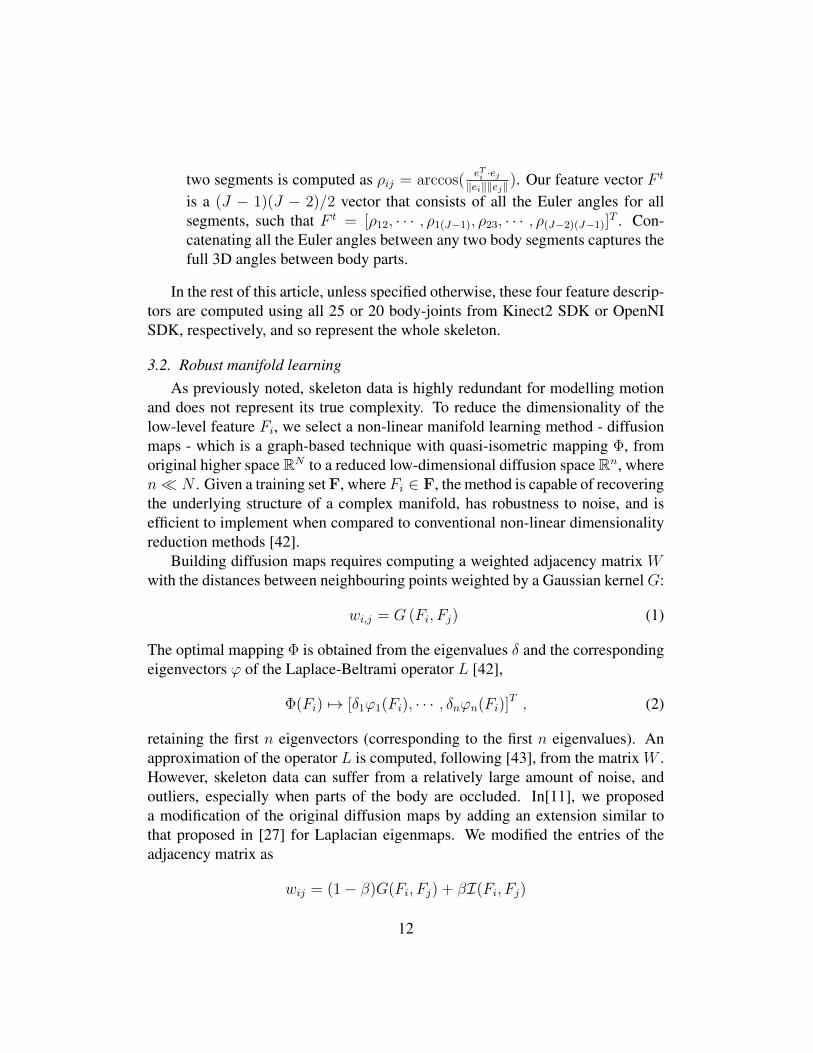
Figure 3: First dimension of gait data in reduced space, using JP low-level feature. (a) originaldiffusion maps according to [27], (b) robust diffusion maps according to [11].

with I(Fi, Fj) =

{1, Fi ∈ Ki or Fj ∈ Kj0, otherwise

(3)

where Ki is a set of neighbours of Fi, and I(�) is an indicator function with theweighting factor β that was introduced in [27]. The indicator function avoidsdisconnected components in Laplacian eigenmaps, thus reducing the influence ofoutliers.

Figure 3 illustrates the first dimension of the dimensionality reduced JP datafor gait, clearly indicating that the original diffusion maps could not capture theintrinsic cyclic nature of the gait, while the robust diffusion maps method bettercaptures the periodicity of the walking cycles.

Mapping testing data - The Nystrom extension [44] extends the low dimensionalrepresentation computed from a training set to new samples, by evaluating themapping of a new data F t as

Φ′k(Ft) =

∑Fi∈F

L(F t, Fi)ϕk(Fi) (4)

with Φ′k(Ft) the kth component of Φ′(F t), k = 1 · · ·n. The operator L(F t, Fi)

is obtained in the same fashion as in [43], but based on our new definition of wijwith the added indicator function I(�). We use this mapping O = Φ′(F t) as ourhigh-level feature for building a motion model.

3.3. Human motion modellingHMM-based methods can efficiently represent temporal dynamics of motion,

and later in Section 5, we show how they naturally can be applied to motion qualityassessment. The term ‘continuous HMM’ is often used to refer to models wherethe observation vector is continuous in Rn [45, 46]. As the observation space

13

is continuous in our case, all the models presented next are in fact ‘continuousHMMs’, but we use only ‘HMM’ for brevity.

Four variations of an HMM-based motion model are explained next in orderof complexity and novelty of usage for human motion modelling. Their maincharacteristics are summarised in Table 1.

Notation We use the following notation throughout the section. Suppose Mis the number of possible states denoted S = {S1 . . . SM}, where the state attime t is qt ∈ S. The M × M transition matrix is A = {aij}, where aij =P (qt = Sj |qt−1 = Si ), and let π = {πi} be an initial state distribution, whereπi = P (q1 = Si). The observation probability distribution is denoted by B ={bj (Ot)}, where bj (Ot) = P (Ot |qt = Sj ) , j = 1 . . . N is the probability of ob-serving Ot when in state Sj . For continuous observations, the observation prob-ability bj(Ot) is defined as a probability density function (PDF). Here, differentcontinuous observation models are used for the four HMMs that we now intro-duce.

a. Classical HMMWe refer to an HMM with continuous observation densities and finite num-

ber of discrete hidden states as a ‘classical’ HMM, in line with [45]. A classi-cal HMM has three basic elements which can be written in a compact form asλa = {A,B, π}. In our implementation, Gaussian mixture models are used as theobservation model:

bj (Ot) =I∑i=1

cjiN (Ot;µji, σji) (5)

with I the number of components in the mixture,∑I

i=1 cji = 1, and cji ≥ 0. SuchHMMs are trained by maximising the probability of the observation sequencesgiven by the model, λa∗ = arg max

λaP (O |λa ), and is solved by the Baum-Welch

method. In testing, the likelihood of a new sequence, given the trained model, iscalculated as,

P (O |λa ) =∑

q1,...,qT

πq1P (O1 |q1 )T∏t=2

P (Ot |qt )P (qt| qt−1) (6)

using the forward algorithm. The ‘classical’ HMM is a parametric model, asthe number of states M needs to be decided a priori, or optimised based on anevaluation set.

14

b. HMM with explicit state duration densityWhen modelling human motion, we note that the time elapsed at each body-

pose configuration can be indicative of the quality of motion. For example, freez-ing during the walking cycle is highly indicative of deteriorating functional mobil-ity, e.g. in Parkinson’s and stroke patients. In classical HMMs, the state duration,i.e. the time elapsed between transiting to a state and transiting out of it, is notmodelled and they would have difficulty discriminating the evolution of the bodymotion through time.

To overcome the problem, and keep the semantic meaning in the latent stateswhile dealing with the lack of transition between them, explicitly modelling thestate duration can help to address the problem [45]. A state duration model can bebuilt asD = {P (d |S1 ) . . . P (d |SM )}, where the state duration for each state Sj ismodelled by the probability density P (d |Sj ). We implement this probability with

a Poisson distribution P (d |Sj ) = P(d; θj) =e−θj θdjd!

, where θj is the mean durationof state Sj . By this definition, the likelihood of a state duration observation dqr attime t depends only on the current state qr and is independent of the duration ofthe previous state.

The probabilities in the trained HMM model are thus expanded to λb = {A,B, π,D},with B implemented as in (5). Again λb is a parametric model with a discretenumber of states M as its parameter. The likelihood of the observed sequenceO = {O1 . . . OT} given the trained model is calculated as,

P (O |λb ) =R∑r=1

∑q1,...,qr

∑d1,...,dr

πq1P (d1|q1)P (O1, . . . , Od1|q1)

r∏i=2

P (qi|qi−1)P (di|qi)P (Oi−1∑k=1

dk+1, . . . , Odi|qi)

(7)

where P (Oi, . . . , Oj|q) =j∏k=i

P (Ok|q), and r is the number of different states

reached during the sequence, restricted to a minimum R = d TDe in case of a

maximum state durationD. As with classical HMMs, the likelihood of a sequencecan be obtained using the forward algorithm.

c. HMM with a discriminative classifierClassical HMM has been employed efficiently when the motion can be broken

into distinct sub-motions [47, 46]. However, some motions can not be automati-cally divided into such sub-motions by the training of the conventional Gaussian

15

mixture-based observation model, and require uniformly splitting the motion cy-cles in training sequences into M manually defined states. For a smooth motion(e.g. walking), such splitting of the motion cycle may lead to poor discrimina-tion between the states when training the observation model. To avoid this, thetraditional Gaussian mixture-based observation model could be replaced by a dis-criminative classifier which is trained to discriminate the poses of one state fromanother.

Given a set of extracted features from the training data, the objective is tobuild a suitable classifier which better discriminates the data. In this work, SVMsas large margin classifiers are used, although other classifiers could also be em-ployed. Combining SVMs with HMMs has been previously applied, e.g. inspeech recognition [48] and facial action modelling [49], where the posterior classprobability is approximated by a sigmoid function [50]. We employ this hybridclassification method for our observation model, following [49] where the multi-class SVM is implemented using one-versus-one approach. In total, M(M−1)/2SVMs are trained for the pairwise classification representing all possible pairs outofM classes. For each SVM, pairwise class probability αij = P (Si|Si or Sj, Ot)is calculated using Platt’s method [51]. Such pairwise probabilities are trans-formed into posterior probabilities as,

P (qt = Sj|Ot) = 1/

[M∑

j=1,j 6=i

1

αij− (M − 2)

]. (8)

The continuous observation probabilities bj(Ot) are formed by the posterior prob-abilities using Bayes’ rule,

bj(Ot) ∝ P (qt = Sj|Ot)/P (qt = Sj) . (9)

Similar to classical HMMs, the discriminative approach is parametric and re-lies on the number of states M . The model λc = {A,B, π} does not differ fromλa in training or testing, but the observation model is based on the discriminativeclassifier.

d. Continuous-state HMMIn the previous model λc, the hidden state represents the proportion of motion

completion at the current frame, which is by nature continuous. Thus in [11],we proposed a statistical model that described continuous motion completion, asan approach that is highly suited to motion quality assessment. This model is in

16

effect a continuous-state HMM, and we represent it here from that perspective.Continuous-state HMMs have been widely used in signal processing in general,for example in [52] where a continuous-state HMM model of deforming shapeswas implemented for monitoring crowd movements.

We introduced in [11] the continuous variable X with value xt ∈ [0, 1] todescribe the progression of motion, i.e. the proportion of motion completed atframe t which linearly increases from 0 at the start of the motion to 1 at its end.For periodic motions, xt is analogous to the motion’s phase, and increases withinone cycle of the motion, and then resets to 0 for the next cycle. The hidden stateof our continuous-state HMM is then qt = xt.

The crucial advantage of using this continuous state variable is that the motiondoes not have to be discretized into a number of segments, the model is non-parametric, and the problem of choosing an optimal M becomes irrelevant. How-ever, the infinite number of possible states makes the commonly used approachesfor training an HMM and evaluating an observation sequence impractical sincethese algorithms are based on integrating over a finite number of possible states.Thus, novel algorithms were introduced in [53, 52], e.g. based on particle filter-ing. Our model differs from these HMMs, both in the definition of the observationmodel and state transition probabilities, and in the algorithms used to perform thetraining and evaluation.

In our continuous-state HMM, the observation model is the PDF bxt(Ot) =fOt(Ot|qt = xt). We learn this probability from training data as

fOt(Ot|qt = xt) =fOt,xt(Ot, xt)

fxt(xt), (10)

using a Parzen window estimator. The kernel bandwidth of the estimator is aparameter of this method that we set empirically so as to avoid over-smoothingof the PDFs. Learning the observation model requires knowing or estimating xtfor the training data. For simplicity, we assume that our training data representsmotions with uniform dynamics (i.e. uniform speed within motion or motioncycle), and we compute xt proportional to time. An example observation modelPDF is shown in Fig. 4 for the motion of ascending stairs.

We define the transition model A analytically as the PDF

fxt (xt|xt−1) =1

σ√

2πe−

12(∆xt−v∆τt

σ )2

, (11)

where ∆xt = xt − xt−1, τt is the time at frame t, and ∆τt = τt − τt−1. Thistransition model thus assumes proportionality between the proportion of motion

17

Figure 4: Example of PDF that defines the observation model in model λd. The plot shows themarginal of the PDF for the first manifold dimension.

completion x and time τ . v is the speed of the motion and is estimated as

v =1

N

N∑i=1

∆xi∆τi

, (12)

so that the model adapts to different motion speeds. During training, v is com-puted for the complete motion or motion cycle. When evaluating a test sequence,v is computed within a sliding window in order to handle sequences with non-constant speeds, although its values are kept within empirically determined limitsfor a normal movement. The size of the window will be discussed later in thissection. The standard deviation σ in (11) modulates the constraint that ∆x is pro-portional to ∆τ . Its choice has been determined empirically so as to enforce astrong constraint when evaluating the probability of a sequence (σeval = 10−3),and a weaker constraint (σest = 7e−3) when estimating xt. This relaxation of theproportionality constraint when estimating xt aims at increasing flexibility of themodel to describe motion dynamics that deviate from normal due to significantspeed variations. Note that such abnormal motions would still be penalised bysignificantly lower probabilities P (O|λd) due to the lower σeval.

To summarise, the continuous-state HMM, first proposed in a different for-mulation as a statistical model in [11], is defined by λd = {A,B, π} where Ais defined analytically and B is estimated from training data. The initial statedistribution π is uniform to enable evaluation from any point in the motion.

Similarly to finite state HMMs, the likelihood of a sequence of observationsO = {O1 . . . OT} under model λd is an integration over all possible values for the

18

hidden states

P (O|λd) =

∫{x1,...,xT }

fO,x1,...,xT (O, x1, . . . , xT )

=

∫{x1,...,xT }

fx1 (x1) fO1 (O1|x1)T∏i=2

fOi (Oi|xi) fxi (xi|xi−1) .(13)

The derivation of (13), that exploits Markovian properties, can be found in [11].Such an integral over an infinite number of possibilities is impractical to com-

pute. The approximation we present next allows reducing (13) to a more easilysolvable form. From our definition of the transition model in (11), given a valuext−1 of variable X at frame t − 1, its value xt at frame t follows a normal dis-tribution around xt−1 + v∆τt with standard deviation σ. In the ideal case of aperfectly normal motion, σ should tend to 0 and the normal distribution wouldtend to a Dirac distribution. For σ small enough, that is to say for a strong enoughconstraint on the evolution of X during the motion, we can use the approximationσ ≈ 0, which leads to

P (O|λd) ≈ fx1 (x1) fO1 (O1|x1)T∏i=2

fOi (Oi|xi) fxi (xi|xi−1) . (14)

The notation xi highlights that this value is the most likely for X at frame i givenxi−1 and ∆τi , i.e. xi = xi−1 + v∆τi .

When computing P (O|λd) using this approximation, the values xi need to beestimated. This can be done by maximising their likelihood conditional on thesequence of observations:

{x1, . . . , xT} = arg maxx1,...,xT

fx1,...,xT (x1, . . . , xT |O)

= arg maxx1,...,xT

fO,x1,...,xT (O, x1, . . . , xT )

fO (O1, . . . , Ot)

= arg maxx1,...,xT

fx1 (x1) fO1 (O1|x1)T∏i=2

fOi (Oi|xi) fxi (xi|xi−1) .

(15)

In our implementation, this estimation is performed using unconstrained nonlinearoptimisation. Similar to the estimation of v, and for the sake of efficiency, we

19

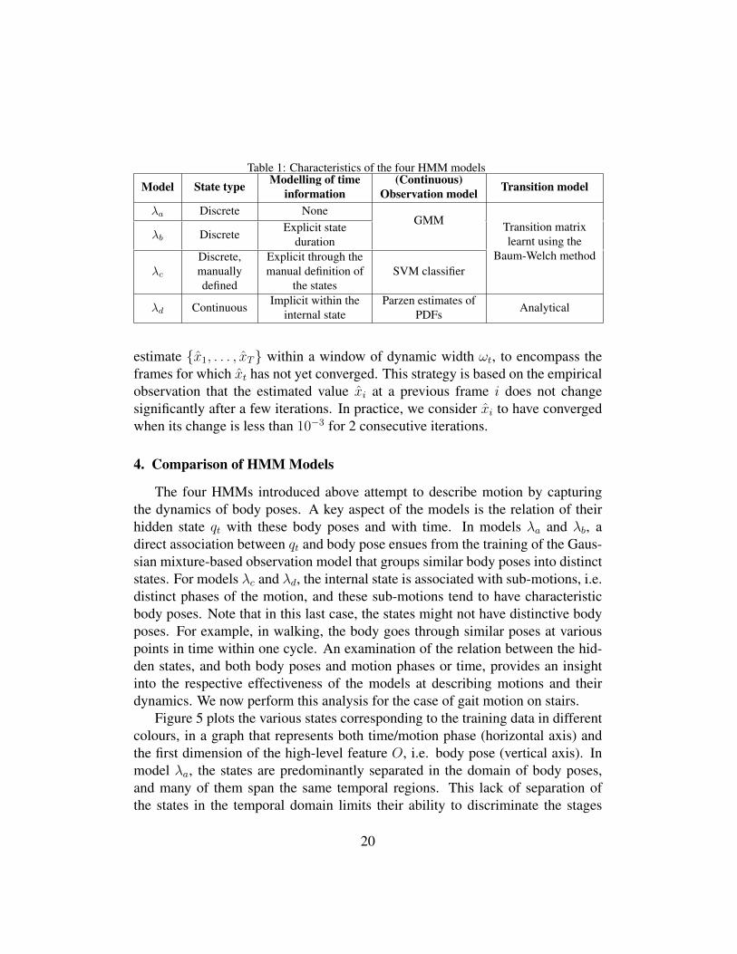
Table 1: Characteristics of the four HMM models

Model State type Modelling of timeinformation

(Continuous)Observation model Transition model

λa Discrete NoneGMM Transition matrix

learnt using theBaum-Welch method

λb Discrete Explicit stateduration

λc

Discrete,manuallydefined

Explicit through themanual definition of

the statesSVM classifier

λd Continuous Implicit within theinternal state

Parzen estimates ofPDFs Analytical

estimate {x1, . . . , xT} within a window of dynamic width ωt, to encompass theframes for which xt has not yet converged. This strategy is based on the empiricalobservation that the estimated value xi at a previous frame i does not changesignificantly after a few iterations. In practice, we consider xi to have convergedwhen its change is less than 10−3 for 2 consecutive iterations.

4. Comparison of HMM Models

The four HMMs introduced above attempt to describe motion by capturingthe dynamics of body poses. A key aspect of the models is the relation of theirhidden state qt with these body poses and with time. In models λa and λb, adirect association between qt and body pose ensues from the training of the Gaus-sian mixture-based observation model that groups similar body poses into distinctstates. For models λc and λd, the internal state is associated with sub-motions, i.e.distinct phases of the motion, and these sub-motions tend to have characteristicbody poses. Note that in this last case, the states might not have distinctive bodyposes. For example, in walking, the body goes through similar poses at variouspoints in time within one cycle. An examination of the relation between the hid-den states, and both body poses and motion phases or time, provides an insightinto the respective effectiveness of the models at describing motions and theirdynamics. We now perform this analysis for the case of gait motion on stairs.

Figure 5 plots the various states corresponding to the training data in differentcolours, in a graph that represents both time/motion phase (horizontal axis) andthe first dimension of the high-level feature O, i.e. body pose (vertical axis). Inmodel λa, the states are predominantly separated in the domain of body poses,and many of them span the same temporal regions. This lack of separation ofthe states in the temporal domain limits their ability to discriminate the stages

20

5 states 7 states 10 states 15 states

λa

λb

λc

Continuous state

λd

Figure 5: States defined in models λa (top row), λb (2nd row), λc (3rd row), and λd (bottom row).For the discrete models (λa-λc), colours denote different states, while for the continuous model(λd) continuous colour gradient is used based on the value of the internal state.

21

of the motion. As another consequence, transition between different states is notnecessary for motion evolution. This may lead to poor modelling of the dynamicsof the motion, as will be shown in Section 6 where freezes of gait often cannot bedetected by model λa. Note in Fig. 5 that increasing the number of states M doesnot significantly improve the description of dynamics as the additional separationis predominantly in the domain of body pose O than in the motion phase/timedomain.

The explicit modelling of state duration in model λb addresses the problem ofstate stagnation in model λa. Although the possible states are still badly separatedin the temporal domain, as seen in Fig. 5, the explicit modelling of state durationenables model λb to better describe the dynamics of motions, and in particular todetect freezes of gaits.

Another way of addressing the issues of model λa is to define the hidden statesas corresponding to distinct temporal regions, by manually dividing a motion uni-formly into equal-length segments. This is the strategy used in model λc. Notethat, depending on the type of motion, several of the resulting states may corre-spond to similar body poses. This is for example the case of gait, as discussedearlier and illustrated in Fig. 5 where several distinct states are located in thesame region of the embedded space. Consequently, as mentioned in Section 3.3c,the observation model produced by the classical HMM training algorithm maybe poorly discriminative, and requires to be replaced by a more robust classifier.It should be stressed that the number of possible states significantly impacts theability of such a model to represent the temporal dynamics of the motion. Indeed,in a model with too few possible states, the probability of staying in a well pop-ulated state may be higher than transiting to the next one, resulting in the samestate stagnation problem than in model λa. On the other hand, when the number ofpossible states is too high, the body poses of distinct states may become too simi-lar and overcome the discrimination power of the classifier, leading to a reductionin performance. This is illustrated in Fig. 6(c), where the best ROC curves areobtained for 15 to 30 states, while deteriorating quickly when the state is less than10 or higher than 40. Further, discriminative classifiers, such as SVMs, cannotnaturally handle unknown observations, and would therefore not clearly attributea state to an unusual observed body pose.

We note in model λc that an increase in the number of states (while remainingwithin the ”discriminative zone” of the classifier) leads to a better representationof the dynamics of the motion. Model λd extends this idea by having a continuousstate, thus imposing an infinite number of possible states. Its observation modeldoes not rely on a discriminative classifier, but instead it exploits non-parametric

22

estimations of conditional PDFs, as explained in Section 3.3d. When two or moresignificantly different states are equally probable given an observation, as for ex-ample in the gait model of Fig. 4, model λd relies on the relative rigidity of itstransition model to handle these ambiguities.

5. Quality assessment measures

Using any one of our four models trained on normal motion sequences, onecan detect anomalies in new observations and assess the quality of the motionbased on the likelihood of the new observation to be described by the model. Anonline assessment of the motion, computed on a frame-by-frame basis, would bedesirable for triggering timely alerts when the observed motion drops below athreshold in its level of normality. A straightforward way of obtaining an onlinemeasure would be to compute the likelihood P (O|λi) within a sliding window.However, this strategy may prove to be difficult to apply, as the choice of windowsize requires a delicate compromise between a sufficient number of frames, inorder to capture and analyse the dynamics of the movement, and a small enoughwindow so as to preserve the instantaneous properties of an online measure. More-over, this window size would have to be adjusted for each type of motion, and alsofor instances of a motion performed at significantly different speeds.

To overcome these problems, we propose a dynamic measure

Mt = logP (Ot|O1, . . . , Ot−1, λi) , (16)

that is the log-likelihood of the current frame given the previous frames and themodel. For models λa, λb, and λc, P (Ot|O1, . . . , Ot−1, λi) may be simply com-puted as P (O|λi)

P (O1,...,Ot−1|λi) using two calls to the forward algorithm. In the case ofmodel λd, this measure can only be obtained after the convergence of xt, andP (Ot|O1, . . . , Ot−1, λi) may be calculated using the approximation of (14) asfOt (Ot|xt) fxt (xt|xt−1).

In [11], we proposed a similar online measure, that instead of waiting for theconvergence of xt, integrated P (Ot|O1, . . . , Ot−1, λi) over the dynamic slidingwindow of size ωt which was defined for model λd in Section 3.3d., in order to

23

account for the updated values of xt that are re-estimated within the window:

Mωt =t∑

j=tmin

logP (Oj|O1, . . . , Oj−1, λi)

= logt∏

j=tmin

P (Oj|O1, . . . , Oj−1, λi)

= logt∏

j=tmin

P (O1, . . . , Oj, λd)

P (O1, . . . , Oj−1, λi)

= logP (O1, . . . , Ot, λd)

P (O1, . . . , Otmin−1, λi)

= logP (Otmin , . . . , Ot|O1, . . . , Otmin−1, λi) ,

(17)

with tmin the first frame of the sliding window. Thus Mωt can be seen as thelog-likelihood of the sliding window given the previous observations. This con-ditionality in the probability alleviates the effect of the window size that we dis-cussed earlier. In our experiments, for convenience and efficiency, we limit ωt to amaximum of 15 frames, although it rarely goes above 10 frames. For models λa,λb, and λc, the forward algorithm does not require the estimation of xt as it sumsprobabilities over all possible states, so the value of ωt cannot be determined auto-matically. Instead, we set it to a constant value ω, and we explore the influence ofits choice on the results in Section 6, where we shall also compare our two onlinemeasuresMt andMωt .

In addition to these two measures of dynamics quality, we also proposed in[11] a measure of pose quality, computed independently for each frame as:

Mpose = log fOi (Oi) . (18)

6. Experimental evaluation

To demonstrate the performance of the motion quality analysis framework, weanalysed the motions of walking on a flat surface, gait on stairs, and transitionsbetween sitting and standing, which are particularly critical for rehabilitation mon-itoring in patients with musculoskeletal disorders, disease progression in PD pa-tients, and for many others. For the analysis of such motions, we compared differ-ent low-level features, dimensions of the manifold embedding, and motion mod-els, as proposed in Sections 3.1 to 3.3 respectively. We also investigated whether

24

full-body information is consistently needed for all tested movement types. Wetested gait on stairs on the dataset SPHERE-staircase2014 (first introduced in [11])as well as two new datasets SPHERE-Walking2015 and SPHERE-SitStand2015for the assessment of gait on a flat surface and of sitting and standing movementsrespectively3. The datasets were used to perform abnormality detection by apply-ing the online measuresMt (Eq.16) andMwt (Eq.17), both on a frame-by-framebasis and for the whole sequence.

6.1. DatasetsSPHERE-Staircase2014 dataset [11] – This dataset includes 48 sequences of12 individuals walking up stairs, captured by an Asus Xmotion RGB-D cameraplaced at the top of the stairs in a frontal and downward-looking position. Itcontains three types of abnormal gaits with lower-extremity musculoskeletal con-ditions, including freezing of gait (FOG) and using a leading leg, left or right,in going up the stairs (i.e. LL or RL respectively). All frames have been manu-ally labelled as normal or abnormal by a qualified physiotherapist. We used 17sequences of normal walking from 6 individuals for building the model and 31sequences from the remaining 6 subjects with both normal and abnormal walkingfor testing.

SPHERE-Walking2015 dataset – This dataset includes 40 sequences of 10 indi-viduals walking on a flat surface. This dataset was captured by an Asus XmotionRGB-D camera placed in front of the subject. It contains normal gaits and twotypes of abnormal gait, simulating, under the guidance of a physiotherapist, strokeand Parkinson disease patients’ walking. We used 18 sequences of normal walk-ing from 6 individuals for building the model, and 22 sequences from 4 othersubjects with both normal and abnormal gaits for testing. The testing set includes5 normal, 8 Parkinson, and 9 Stroke sequences.

SPHERE-SitStand2015 dataset – This dataset includes 109 sequences of 10 in-dividuals sitting down and standing up in a home environment. Since the AsusXmotion RGB-D camera is unable to track the skeleton for movements that causeself-occlusions, the data was captured using a Kinect 2 camera instead. It containsnormal and two types of abnormal motions, including (a) restricted knee and re-stricted hip flections and (b) freezing. We used 9 sequences of normal movement

3To be released to the public domain soon.

25

from 8 individuals for building each sitting and standing model, and 91 sequencesfrom two other subjects with normal and abnormal movements for testing, includ-ing 31 normal and 12 abnormal sitting, and 36 normal and 12 abnormal standing.The abnormal sequences comprise 4 samples of each abnormality type.

In the following experiments, we first compare the methods on the SPHERE-Staircase2014 dataset. Then, we show that the methods can be extended to othertypes of human motion, both periodic and non-periodic, using the SPHERE-Walking2015 and SPHERE-SitStand2015 datasets.

6.2. Parameter settingNumber of states – Three of the motion models (λa, λb and λc) are paramet-

ric, expecting the number of states M to be identified in advance. It is commonlyknown that classical HMM models are sensitive to the number of states. To selectthe appropriate number, we plotted our results as ROC curves of frame classifica-tion accuracy using our online measure on all test sequences for different numbersof states. Fig. 6 shows the ROC curves together with their area under the curve(AUC) values when using feature JP. Both λa and λb models seem insensitive tothe number of states, especially when M ≥ 5. The performance of motion modelλc is highly sensitive to the number of states with significantly improved perfor-mance for 10 < M < 40. As discussed in Section 4, this is as expected, sincewalking cycles are uniformly divided into several states, and fewer states may leadto high probabilities of self-transitions which would then fail to explain the tem-poral evolution of the motion. On the other hand, having a relatively larger valueof M may cause difficulty in discriminating data, thus leading to poor recognitionresults.

To choose the optimal number of states, the model with the maximal value ofAUC was selected. We followed the same process to obtain the optimal number ofstates for low-level features JV, PJD, and PJA for each of the discrete-state HMMs,as summarised in Table 2 Model λd does not require optimizing the number ofstates, since its hidden variable is continuous.

Temporal window size – ωt is also a parameter for models λa, λb, and λc(see Section 5). We investigated the effects of different temporal window sizeson the detection accuracy when computingMωt . We chose the optimal settings(feature type and the number of states) that provided the best results for each ofthe models and tested with different temporal window sizes set to 1, 5, 10, 15, 20and 25 frames. This test was not performed for model λd as ωt is set dynamicallyfor that model (see Section 3.3d. for details).

26

0 0.2 0.4 0.6 0.8 10

0.2

0.4

0.6

0.8

1

false positive rate

true

pos

itive

rat

e

3 states − 0.404 states − 0.305 states − 0.327 states − 0.3710 states − 0.3615 states − 0.33

(a) model λa

0 0.2 0.4 0.6 0.8 10

0.2

0.4

0.6

0.8

1

false positive ratetr

ue p

ositi

ve r

ate

3 states − 0.674 states − 0.665 states − 0.657 states − 0.6710 states − 0.6715 states − 0.66

(b) model λb

0 0.2 0.4 0.6 0.8 10

0.2

0.4

0.6

0.8

1

false positive rate

true

pos

itive

rat

e

3 states − 0.385 states − 0.357 states − 0.4010 states − 0.6220 states − 0.7330 states − 0.7340 states − 0.6450 states − 0.53

(c) model λc

Figure 6: Frame classification accuracy for gait on stairs: ROC curves using our online measureMωt for different number of states for feature type JP.

Table 2: Optimal number of states for each low-level feature for each discrete-state HMM (modelsλa, λb,λc) and motion type. For the continuous-state HMM (model λd), the number of states isundefined and hence the parameter is not applicable (N/A). For gait on flat surface, sitting, andstanding motions, only models λc and λd were evaluated.

Motion Motion model JP JV PJD PJA

Gait on stairsλa 3 4 3 3λb 3 3 4 4λc 20 20 20 15

Walking on a flat surface λc 15 5 5 7Sitting λc 10 7 7 5

Standing λc 15 15 5 7All λd N/A N/A N/A N/A

As shown in Table 3, the best results for model λa, λb and λc for gait onstairs were obtained with a temporal window size of 15 frames, although smallernumber of frames, such as 5 or 10, are not far in performance. Selecting too smalla size of window may allow the noise to prevent capturing the abnormality of aframe, while too large a window may include both abnormal and normal frameswithin the window and would thus fail to detect the abnormality.

Choice of online measure – As discussed earlier, models λa, λb, and λc ob-tained the best results when computing measure Mωt with a temporal windowsize of 15 frames. The measureMt is equivalent toMωt at a window size of 1frame (as in the 1st column of Table 3). The often worse results achieved withMt for models λa, λb, and λc were caused by errors obtained from unsmoothed

27

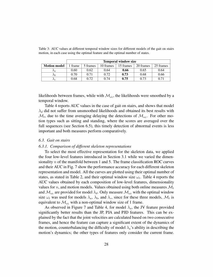
Table 3: AUC values at different temporal window sizes for different models of the gait on stairsmotion, in each case using the optimal feature and the optimal number of states.

Temporal window sizeMotion model 1 frame 5 frames 10 frames 15 frames 20 frames 25 frames

λa 0.60 0.62 0.64 0.66 0.65 0.64λb 0.70 0.71 0.72 0.73 0.68 0.66λc 0.68 0.72 0.74 0.75 0.73 0.71

likelihoods between frames, while withMωt , the likelihoods were smoothed by atemporal window.

Table 4 reports AUC values in the case of gait on stairs, and shows that modelλd did not suffer from unsmoothed likelihoods and obtained its best results withMt, due to the time averaging delaying the detections of Mωt . For other mo-tion types such as sitting and standing, where the scores are averaged over thefull sequences (see Section 6.5), this timely detection of abnormal events is lessimportant and both measures perform comparatively.

6.3. Gait on stairs6.3.1. Comparison of different skeleton representations

To select the most effective representation for the skeleton data, we appliedthe four low-level features introduced in Section 3.1 while we varied the dimen-sionality n of the manifold between 1 and 5. The frame classification ROC curvesand their AUC in Fig. 7 show the performance accuracy for each different skeletonrepresentation and model. All the curves are plotted using their optimal number ofstates, as stated in Table 2, and their optimal window size ωt. Table 4 reports theAUC values obtained by each composition of low-level features, dimensionalityvalues for n, and motion models. Values obtained using both online measuresMt

andMωt are provided for model λd. Only measureMωt with the optimal windowsize ωt was used for models λa, λb, and λc, since for these three models, Mt isequivalent toMωt with a non-optimal window size of 1 frame.

As observed in Figure 7 and Table 4, for model λa, the JV feature providedsignificantly better results than the JP, PJA and PJD features. This can be ex-plained by the fact that the joint velocities are calculated based on two consecutiveframes, and hence the feature can capture a significant extent of the dynamics ofthe motion, counterbalancing the difficulty of model λa’s ability in describing themotion’s dynamics; the other types of features only consider the current frame.

28

0 0.2 0.4 0.6 0.8 10

0.2

0.4

0.6

0.8

1

false positive rate

true

pos

itive

rat

e

JP − 0.40JV − 0.63PJD − 0.46PJA − 0.56

(a) model λa

0 0.2 0.4 0.6 0.8 10

0.2

0.4

0.6

0.8

1

false positive rate

true

pos

itive

rat

e

JP − 0.67JV − 0.64PJD − 0.70PJA − 0.64

(b) model λb

0 0.2 0.4 0.6 0.8 10

0.2

0.4

0.6

0.8

1

false positive rate

true

pos

itive

rat

e

JP − 0.73JV − 0.62PJD − 0.75PJA − 0.61

(c) model λc

0 0.2 0.4 0.6 0.8 10

0.2

0.4

0.6

0.8

1

false positive rate

true

pos

itive

rat

e

JP − 0.82JV − 0.65PJD − 0.83PJA − 0.69

(d) model λd

Figure 7: Comparison of different skeleton representations (low-level features with their respectiveoptimal manifold dimensionality) for models (a) λa, (b) λb, (c) λc, and (d) λd, at abnormal framedetection for the gait on stairs movement. The plots are for the optimal state numbers (see Table2) and online measure for each model:Mωt with ωt = 15 for models λa, λb, and λc, andMt formodel λd.

For model λb, there was no remarkably significant variation in the results for thedifferent features, however, the PJD feature performed best across all dimensions.For model λc, again PJD provided the best outcome in all dimensions. Further,Table 4 shows that for all the best results of the three discrete models λa, λb, andλc, the accuracy does not depend strongly on the dimensionality of data. In sum-mary, we chose the JV feature for model λa and PJD feature for models λb and λcwith the first 3 manifold dimensions as the optimum skeleton representation forthese three models, as highlighted in Table 4.

For model λd, although the best result in Table 4 was for the PJD feature in

29

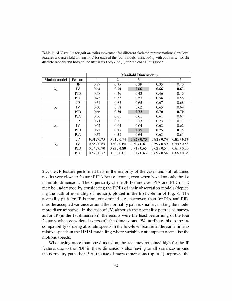
Table 4: AUC results for gait on stairs movement for different skeleton representations (low-levelfeatures and manifold dimensions) for each of the four models, usingMωt

with optimal ωt for thediscrete models and both online measures (Mt /Mωt ) for the continuous model.

Manifold Dimension nMotion model Feature 1 2 3 4 5

JP 0.37 0.35 0.39 0.35 0.40λa JV 0.64 0.60 0.66 0.66 0.63

PJD 0.38 0.36 0.43 0.46 0.46PJA 0.43 0.52 0.53 0.58 0.56JP 0.64 0.62 0.65 0.67 0.68

λb JV 0.60 0.58 0.62 0.65 0.64PJD 0.66 0.70 0.73 0.70 0.70PJA 0.56 0.61 0.61 0.61 0.64JP 0.71 0.71 0.73 0.73 0.73

λc JV 0.62 0.64 0.64 0.62 0.62PJD 0.72 0.75 0.75 0.75 0.75PJA 0.57 0.58 0.64 0.63 0.61JP 0.81 / 0.75 0.81 / 0.74 0.82 / 0.75 0.81 / 0.74 0.81 / 0.74

λd JV 0.65 / 0.65 0.60 / 0.60 0.60 / 0.61 0.59 / 0.59 0.59 / 0.58PJD 0.74 / 0.70 0.83 / 0.80 0.74 / 0.65 0.62 / 0.54 0.61 / 0.50PJA 0.57 / 0.57 0.63 / 0.61 0.67 / 0.63 0.69 / 0.64 0.66 / 0.65

2D, the JP feature performed best in the majority of the cases and still obtainedresults very close to feature PJD’s best outcome, even when based on only the 1stmanifold dimension. The superiority of the JP feature over PJA and PJD in 1Dmay be understood by considering the PDFs of their observation models (depict-ing the path of normality of motion), plotted in the first column of Fig. 8. Thenormality path for JP is more constrained, i.e. narrower, than for PJA and PJD,thus the accepted variance around the normality path is smaller, making the modelmore discriminative. In the case of JV, although the normality path is as narrowas for JP (in the 1st dimension), the results were the least performing of the fourfeatures when considered across all the dimensions. We attribute this to the in-compatibility of using absolute speeds in the low-level feature at the same time asrelative speeds in the HMM modelling where variable v attempts to normalise themotions speeds.

When using more than one dimension, the accuracy remained high for the JPfeature, due to the PDF in these dimensions also having small variances aroundthe normality path. For PJA, the use of more dimensions (up to 4) improved the

30

1st dimension 2nd dimension 3rd dimension

JP

JV

PJA

PJD

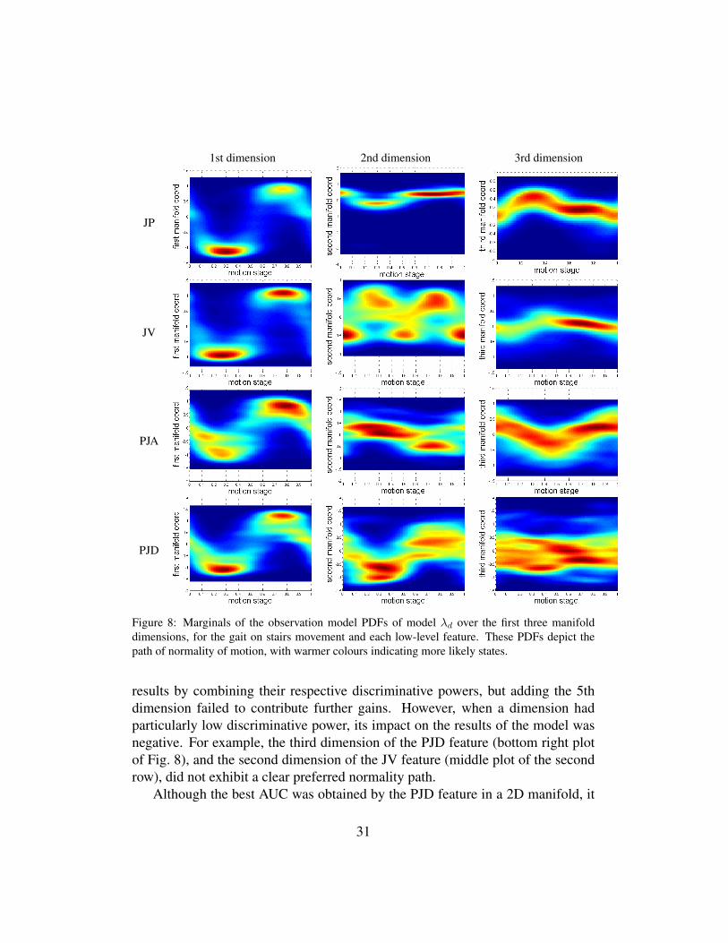
Figure 8: Marginals of the observation model PDFs of model λd over the first three manifolddimensions, for the gait on stairs movement and each low-level feature. These PDFs depict thepath of normality of motion, with warmer colours indicating more likely states.

results by combining their respective discriminative powers, but adding the 5thdimension failed to contribute further gains. However, when a dimension hadparticularly low discriminative power, its impact on the results of the model wasnegative. For example, the third dimension of the PJD feature (bottom right plotof Fig. 8), and the second dimension of the JV feature (middle plot of the secondrow), did not exhibit a clear preferred normality path.

Although the best AUC was obtained by the PJD feature in a 2D manifold, it

31

was only marginally higher than for JP in a 3D manifold, and the ROC curve for JPindicates consistently better performance than that of PJD’s (see Fig. 7(d)). Hence,to conclude, we chose the JP feature for model λd with 3 manifold dimensions asthe optimum skeleton representation (keeping consistency on all four models).

The average processing time (in milliseconds per frame) for building high-level features are 1.18, 1.14, 10.06 and 29.32 for JP, JV, PJD and PJA features,respectively. The experiments were performed using Matlab on a workstationwith an Intel I7-3770S CPU 3.1GHz processor and 8GB RAM. The number ofdimensions of the manifold does not affect the processing time, since its selectionis performed after generating the manifold space.

6.3.2. Comparison of the motion modelsWe evaluated and compared the ability of each model to detect various abnor-

malities in the sequences under optimal parameter settings. Abnormal frameswere detected when the measure of normality, Mωt or Mt , dropped below athreshold. Returning to Fig. 7, it shows the true positive rate against false pos-itive rate at different threshold values. It is clear that model λd performed betterthan the other models at detecting abnormal frames.

Significantly, when an expert, e.g. a physiotherapist, observes a patient, he/sheanticipates a disruption in the normal cycle of gait. This would be before it couldreasonably be identified by an automated system. This is an artefact of usingframe by frame labelling, especially for RL and LL events. When the expert notesa minimal reduction in the speed of the swinging leg, he/she anticipates that theheel strike will not take a place at ‘normal’ position. Hence, the expert classifiesall of the frames leading up to that point as abnormal. However, in terms of thepose trajectory along the manifold, the motion is normal, other than a very subtlereduction in speed. Our approach is robust to subtle changes in gait velocity asthis is present in normal gait as well. Thus, we provide an alternative measureby detecting the abnormality based on the whole event. This motion analysis isstill online, since abnormal events are detected as new frames are being acquired,without having to wait for the full sequence to be available. We first eliminatednoise in the frame classification by removing isolated clusters of less than 3 nor-mal or abnormal frames. Then, we defined an abnormal event as succession of (atleast) 3 consecutive abnormal frames.

We counted as true positive (TP) detections any event that had at least threeframes detected as abnormal, while false negatives (FN) were events with lessthan three detected frames. False positive (FP) detections were either detectedevents that did not intersect by at least three frames with a true abnormal event,

32

or normal periods between abnormal events that had all their frames classified asabnormal. The abnormatity event classification results are illustrated in Fig. 9 andTable 5. Fig. 9 presents precision and recall values when varying the thresholdon the frame classification measure Mωt or Mt , all other parameters being setoptimally for each motion model. Note that this is not the usual Precision againstRecall (PR) plot for event detection, since the threshold we are varying here is noton the measure of likelihood of abnormal event, but on a measure of likelihood ofabnormal frame, hence, the unusual aspect of the plot. Defining a measure of thelikelihood of an abnormal event is not in the scope of this study, but will be thefocus of our future work.

0 0.2 0.4 0.6 0.8 10

0.1

0.2

0.3

0.4

0.5

0.6

0.7

0.8

0.9

1

Recall

Pre

cisi

on

model λa

model λb

model λc

model λd

0 0.2 0.4 0.6 0.8 10

0.2

0.4

0.6

0.8

1

model λa

Recall

Precision

0 0.2 0.4 0.6 0.8 10

0.2

0.4

0.6

0.8

1

model λb

Recall

Precision

0 0.2 0.4 0.6 0.8 10

0.2

0.4

0.6

0.8

1

model λc

Recall

Precision

0 0.2 0.4 0.6 0.8 10

0.2

0.4

0.6

0.8

1

model λd

Recall

Precision

Figure 9: Upper: Precision and recall values for event detection in the gait on stairs scenario whenvarying the threshold on frame classification, plotted for the best parameter setting for each motionmodel. Bottom: Split of the scatter plot into four, for better visualisation.

For each model, the point closest to the top-right corner of the plot (indicatedwith a square) was chosen as the best precision-recall compromise, and its cor-responding measure threshold was used to obtain the results reported in Table 5.

33

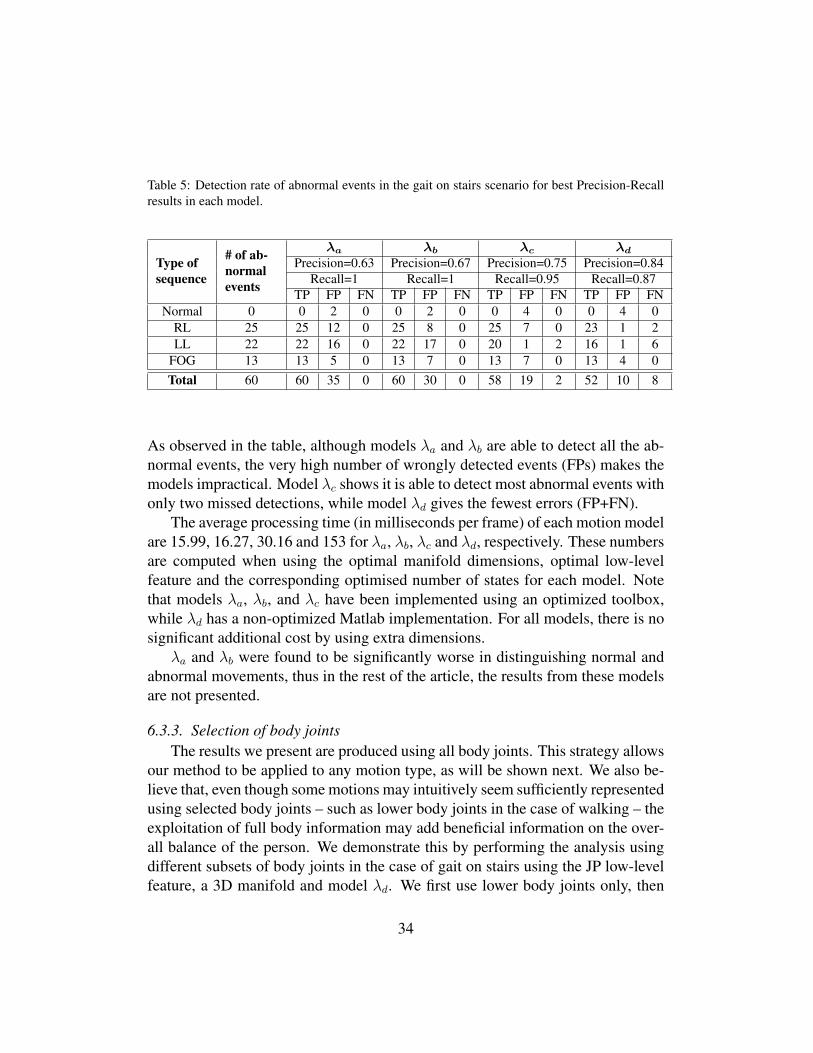
Table 5: Detection rate of abnormal events in the gait on stairs scenario for best Precision-Recallresults in each model.

Type ofsequence

# of ab-normalevents

λa λb λc λd

Precision=0.63 Precision=0.67 Precision=0.75 Precision=0.84Recall=1 Recall=1 Recall=0.95 Recall=0.87

TP FP FN TP FP FN TP FP FN TP FP FNNormal 0 0 2 0 0 2 0 0 4 0 0 4 0

RL 25 25 12 0 25 8 0 25 7 0 23 1 2LL 22 22 16 0 22 17 0 20 1 2 16 1 6

FOG 13 13 5 0 13 7 0 13 7 0 13 4 0Total 60 60 35 0 60 30 0 58 19 2 52 10 8

As observed in the table, although models λa and λb are able to detect all the ab-normal events, the very high number of wrongly detected events (FPs) makes themodels impractical. Model λc shows it is able to detect most abnormal events withonly two missed detections, while model λd gives the fewest errors (FP+FN).

The average processing time (in milliseconds per frame) of each motion modelare 15.99, 16.27, 30.16 and 153 for λa, λb, λc and λd, respectively. These numbersare computed when using the optimal manifold dimensions, optimal low-levelfeature and the corresponding optimised number of states for each model. Notethat models λa, λb, and λc have been implemented using an optimized toolbox,while λd has a non-optimized Matlab implementation. For all models, there is nosignificant additional cost by using extra dimensions.

λa and λb were found to be significantly worse in distinguishing normal andabnormal movements, thus in the rest of the article, the results from these modelsare not presented.

6.3.3. Selection of body jointsThe results we present are produced using all body joints. This strategy allows

our method to be applied to any motion type, as will be shown next. We also be-lieve that, even though some motions may intuitively seem sufficiently representedusing selected body joints – such as lower body joints in the case of walking – theexploitation of full body information may add beneficial information on the over-all balance of the person. We demonstrate this by performing the analysis usingdifferent subsets of body joints in the case of gait on stairs using the JP low-levelfeature, a 3D manifold and model λd. We first use lower body joints only, then

34

in a second test use Orthogonal Marching Pursuit (OMP) to select the low-levelfeatures that are most relevant for deriving the high level features. Fig. 10 showsthat the high level features reconstruction error is dramatically reduced using the 9most significant low-level features, and does not improve significantly using moreof them. Therefore, in our second test we use the 9 most significant low-levelfeatures selected by OMP and summarized in the first row of Table 6. Note thatthese features correspond to both legs and arms data.

Figure 10: Selection of low-level features using the Orthogonal Marching Pursuit: high levelfeature reconstruction error as a function of the number of low-level features.

The ROC curves obtained for frame classification, and the precision and recallvalues for abnormal event detection, are shown for both tests in Fig. 11. The AUCvalues are reported in the second row of Table 6. Our first observation is that,although the best results are obtained using the 21 lower body features, with AUCof 0.74 and 0.77 usingMt andMωt respectively, the only 9 features selected byOMP, and that mix lower and upper body information, are very close with AUC of0.71 for both measures. Secondly, the lower joints results are significantly worsethan the best result of using all body joints that had a AUC of 0.82 usingMt. Weconclude from these two observations that upper body joints contain informationthat may contribute significantly to the analysis of gait and that should not bediscarded.

35

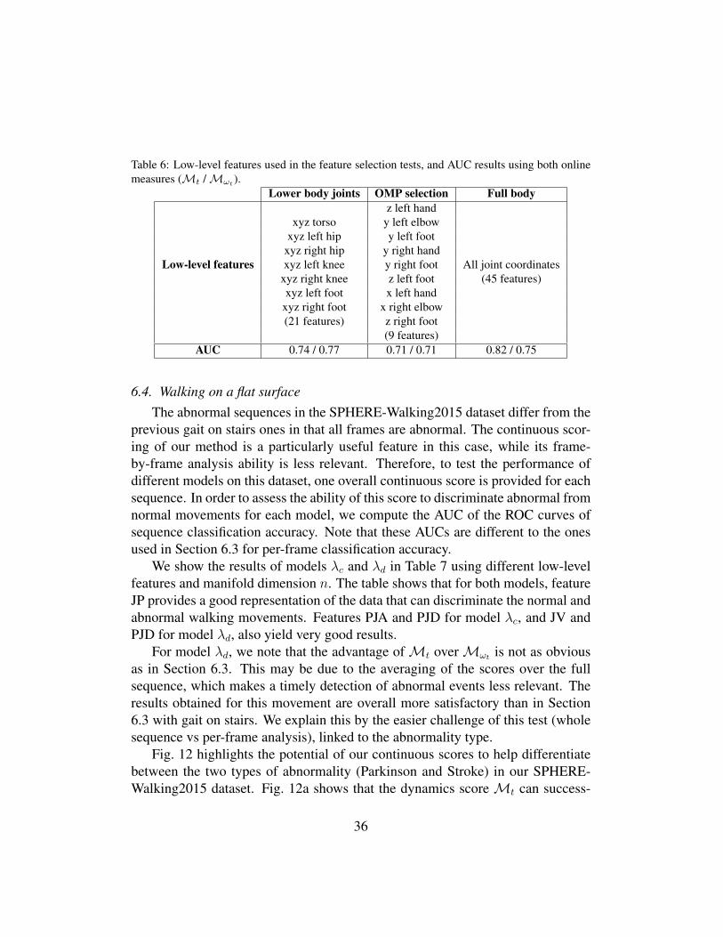
Table 6: Low-level features used in the feature selection tests, and AUC results using both onlinemeasures (Mt /Mωt

).Lower body joints OMP selection Full body

z left handxyz torso y left elbow

xyz left hip y left footxyz right hip y right hand

Low-level features xyz left knee y right foot All joint coordinatesxyz right knee z left foot (45 features)xyz left foot x left hand

xyz right foot x right elbow(21 features) z right foot

(9 features)AUC 0.74 / 0.77 0.71 / 0.71 0.82 / 0.75

6.4. Walking on a flat surfaceThe abnormal sequences in the SPHERE-Walking2015 dataset differ from the

previous gait on stairs ones in that all frames are abnormal. The continuous scor-ing of our method is a particularly useful feature in this case, while its frame-by-frame analysis ability is less relevant. Therefore, to test the performance ofdifferent models on this dataset, one overall continuous score is provided for eachsequence. In order to assess the ability of this score to discriminate abnormal fromnormal movements for each model, we compute the AUC of the ROC curves ofsequence classification accuracy. Note that these AUCs are different to the onesused in Section 6.3 for per-frame classification accuracy.

We show the results of models λc and λd in Table 7 using different low-levelfeatures and manifold dimension n. The table shows that for both models, featureJP provides a good representation of the data that can discriminate the normal andabnormal walking movements. Features PJA and PJD for model λc, and JV andPJD for model λd, also yield very good results.

For model λd, we note that the advantage ofMt overMωt is not as obviousas in Section 6.3. This may be due to the averaging of the scores over the fullsequence, which makes a timely detection of abnormal events less relevant. Theresults obtained for this movement are overall more satisfactory than in Section6.3 with gait on stairs. We explain this by the easier challenge of this test (wholesequence vs per-frame analysis), linked to the abnormality type.

Fig. 12 highlights the potential of our continuous scores to help differentiatebetween the two types of abnormality (Parkinson and Stroke) in our SPHERE-Walking2015 dataset. Fig. 12a shows that the dynamics score Mt can success-

36

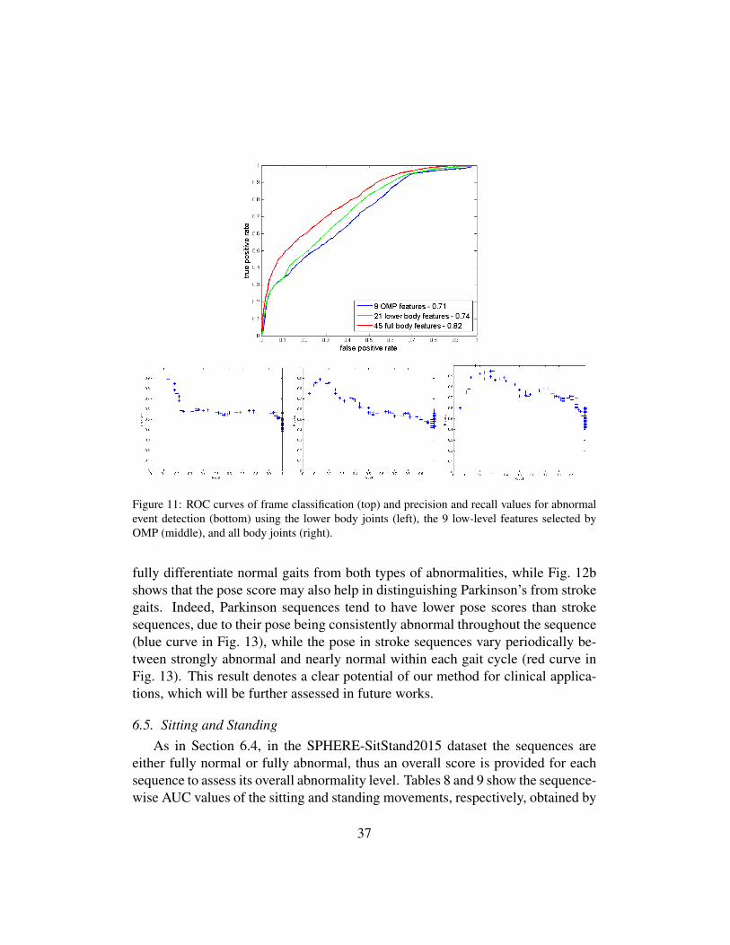
Figure 11: ROC curves of frame classification (top) and precision and recall values for abnormalevent detection (bottom) using the lower body joints (left), the 9 low-level features selected byOMP (middle), and all body joints (right).

fully differentiate normal gaits from both types of abnormalities, while Fig. 12bshows that the pose score may also help in distinguishing Parkinson’s from strokegaits. Indeed, Parkinson sequences tend to have lower pose scores than strokesequences, due to their pose being consistently abnormal throughout the sequence(blue curve in Fig. 13), while the pose in stroke sequences vary periodically be-tween strongly abnormal and nearly normal within each gait cycle (red curve inFig. 13). This result denotes a clear potential of our method for clinical applica-tions, which will be further assessed in future works.

6.5. Sitting and StandingAs in Section 6.4, in the SPHERE-SitStand2015 dataset the sequences are

either fully normal or fully abnormal, thus an overall score is provided for eachsequence to assess its overall abnormality level. Tables 8 and 9 show the sequence-wise AUC values of the sitting and standing movements, respectively, obtained by

37

Table 7: AUC results in the case of the walking on a flat surface motion for different skeletonrepresentations and measures for models λc (Mt) and λd (Mt/Mωt

).Manifold Dimension n

Motion model Feature 1 2 3 4 5

λc

JP 0.96 1.00 0.99 1.00 1.00JV 0.93 0.79 0.86 0.95 0.85PJA 0.91 0.98 1.00 0.96 0.98PJD 1.00 1.00 1.00 1.00 1.00

λd

JP 0.96 / 1.00 0.99 / 1.00 0.95 / 1.00 0.99 / 1.00 0.93 / 1.00JV 0.95 / 0.98 0.88 / 0.86 0.87 / 0.95 0.91 / 0.95 1.00 / 1.00PJA 0.89 / 0.91 0.82 / 0.88 0.91 / 0.96 0.94 / 0.96 0.94 / 0.96PJD 0.96 / 1.00 0.91 / 0.96 0.92 / 0.95 0.89 / 0.93 0.93 / 0.98

(a) (b)

Figure 12: Quality measures for each of the walking sequences: (a) dynamics measureMt, and(b) pose measure Mpose for normal sequences (green), Parkinson sequences (blue), and strokesequences (red).

the different pose representations and motion models. For the sitting motion, bothmodels λc and λd perform better with the JP feature. For the standing motion,model λc also performs better with JP, while model λd should use either JV orPJD. Both models perform similarly well at detecting abnormal sequences, withbest AUCs of model λc at 0.99 and 1.00 for the sitting and standing motionsrespectively, and 1.00 and 0.97 for model λd.

38

Figure 13: Comparison of the pose measureMpose in two examples of Parkinson (blue) and stroke(red) sequences.Mpose is consistently low in the Parkinson sequences, while it varies periodicallyin the stroke one.

Table 8: AUC results in the case of the sitting movement for different skeleton representations andmeasures using models λc (Mt) and λd (Mt/Mωt

).Manifold Dimension n

Motion model Feature 1 2 3 4 5

λc

JP 0.82 0.96 0.99 0.97 0.97JV 0.88 0.87 0.85 0.83 0.77PJA 0.59 0.67 0.68 0.63 0.73PJD 0.80 0.92 0.93 0.92 0.86

λd

JP 0.99 / 1.00 0.99 / 0.99 0.98 / 0.99 0.97 / 1.00 0.95 / 1.00JV 0.69 / 0.73 0.70 / 0.79 0.72 / 0.70 0.71 / 0.66 0.61 / 0.59PJA 0.67 / 0.67 0.61 / 0.56 0.68 / 0.68 0.65 / 0.70 0.62 / 0.66PJD 0.42 /0.47 0.77 / 0.79 0.76 /0.81 0.86 / 0.92 0.81 / 0.85

7. Conclusion

In this work, we have studied the efficiency of different pose representationsand HMM-based dynamics models for describing and assessing the quality offour motions used by clinicians to assess functional mobility. The results showthat the continuous-state HMM is better suited for describing motion dynamicsthan classical, discrete-state HMMs when a frame-by-frame analysis is required.For globally analyzing whole sequences, both the continuous-state HMM and theclassical (discrete-state) HMM with discriminative classifier performed well. Fur-thermore we have found that the adequacy of the pose representation to modellingpose variations plays a key role in the ability of the dynamics model to representand discriminate the motion.

39

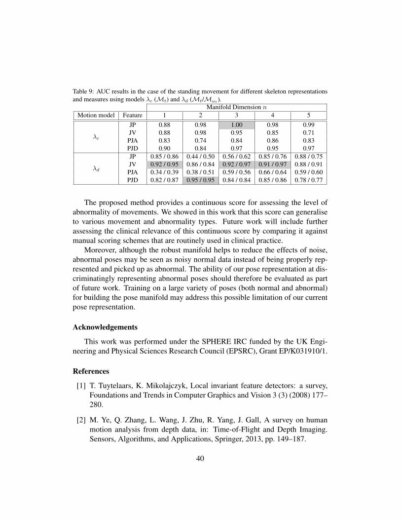
Table 9: AUC results in the case of the standing movement for different skeleton representationsand measures using models λc (Mt) and λd (Mt/Mωt

).Manifold Dimension n

Motion model Feature 1 2 3 4 5

λc

JP 0.88 0.98 1.00 0.98 0.99JV 0.88 0.98 0.95 0.85 0.71PJA 0.83 0.74 0.84 0.86 0.83PJD 0.90 0.84 0.97 0.95 0.97

λd

JP 0.85 / 0.86 0.44 / 0.50 0.56 / 0.62 0.85 / 0.76 0.88 / 0.75JV 0.92 / 0.95 0.86 / 0.84 0.92 / 0.97 0.91 / 0.97 0.88 / 0.91PJA 0.34 / 0.39 0.38 / 0.51 0.59 / 0.56 0.66 / 0.64 0.59 / 0.60PJD 0.82 / 0.87 0.95 / 0.95 0.84 / 0.84 0.85 / 0.86 0.78 / 0.77

The proposed method provides a continuous score for assessing the level ofabnormality of movements. We showed in this work that this score can generaliseto various movement and abnormality types. Future work will include furtherassessing the clinical relevance of this continuous score by comparing it againstmanual scoring schemes that are routinely used in clinical practice.

Moreover, although the robust manifold helps to reduce the effects of noise,abnormal poses may be seen as noisy normal data instead of being properly rep-resented and picked up as abnormal. The ability of our pose representation at dis-criminatingly representing abnormal poses should therefore be evaluated as partof future work. Training on a large variety of poses (both normal and abnormal)for building the pose manifold may address this possible limitation of our currentpose representation.

Acknowledgements

This work was performed under the SPHERE IRC funded by the UK Engi-neering and Physical Sciences Research Council (EPSRC), Grant EP/K031910/1.

References

[1] T. Tuytelaars, K. Mikolajczyk, Local invariant feature detectors: a survey,Foundations and Trends in Computer Graphics and Vision 3 (3) (2008) 177–280.

[2] M. Ye, Q. Zhang, L. Wang, J. Zhu, R. Yang, J. Gall, A survey on humanmotion analysis from depth data, in: Time-of-Flight and Depth Imaging.Sensors, Algorithms, and Applications, Springer, 2013, pp. 149–187.

40

[3] J. Aggarwal, M. S. Ryoo, Human activity analysis: A review, ACM Com-puting Surveys 43 (3).

[4] R. Poppe, A survey on vision-based human action recognition, Image andvision computing 28 (6) (2010) 976–990.

[5] S.-R. Ke, H. L. U. Thuc, Y.-J. Lee, J.-N. Hwang, J.-H. Yoo, K.-H. Choi, Areview on video-based human activity recognition, Computers 2 (2) (2013)88–131.

[6] O. Popoola, K. Wang, Video-based abnormal human behavior recognitiona review, IEEE Transactions on Systems, Man, and Cybernetics, Part C:Applications and Reviews 42 (6) (2012) 865–878.

[7] H. Pirsiavash, C. Vondrick, A. Torralba, Assessing the quality of actions, in:Computer Vision–ECCV 2014, Springer, 2014, pp. 556–571.

[8] R. Wang, G. Medioni, C. Winstein, C. Blanco, Home monitoring musculo-skeletal disorders with a single 3d sensor, in: IEEE Conference on ComputerVision and Pattern Recognition Workshops, IEEE, 2013, pp. 521–528.

[9] J. M. VanSwearingen, K. A. Paschal, P. Bonino, J.-F. Yang, The modifiedgait abnormality rating scale for recognizing the risk of recurrent falls incommunity-dwelling elderly adults, Physical Therapy 76 (9) (1996) 994–1002.

[10] L. Wolfson, R. Whipple, P. Amerman, J. N. Tobin, Gait assessment in theelderly: a gait abnormality rating scale and its relation to falls, Journal ofgerontology 45 (1).

[11] A. Paiement, L. Tao, S. Hannuna, M. Camplani, D. Damen, M. Mirme-hdi, Online quality assessment of human movement from skeleton data, in:British Machine Vision Conference, BMVA press, 2014, pp. 153–166.

[12] M. Z. Uddin, J. T. Kim, T. Kim, Depth video-based gait recognition for smarthome using local directional pattern features and hidden markov model, In-door and Built Environment 23 (1) (2014) 133–140.

[13] J. Shotton, T. Sharp, A. Kipman, A. Fitzgibbon, M. Finocchio, A. Blake,M. Cook, R. Moore, Real-time human pose recognition in parts from singledepth images, Communications of the ACM 56 (1) (2013) 116–124.

41

[14] OpenNI organization, OpenNI User Guide (November 2010).URL http://www.openni.org/documentation

[15] R. Vemulapalli, F. Arrate, R. Chellappa, Human action recognition by rep-resenting 3D skeletons as points in a lie group, in: IEEE Conference onComputer Vision and Pattern Recognition, IEEE, 2014, pp. 588–595.

[16] L. Xia, C.-C. Chen, J. Aggarwal, View invariant human action recognitionusing histograms of 3D joints, in: IEEE Conference onComputer Vision andPattern Recognition Workshops, IEEE, 2012, pp. 20–27.

[17] A. Yao, J. Gall, L. Van Gool, Coupled action recognition and pose estimationfrom multiple views, International journal of computer vision 100 (1) (2012)16–37.

[18] J. Wang, Z. Liu, Y. Wu, J. Yuan, Mining actionlet ensemble for action recog-nition with depth cameras, in: IEEE Conference on Computer Vision andPattern Recognition, IEEE, 2012, pp. 1290–1297.

[19] G. S. Parra-Dominguez, B. Taati, A. Mihailidis, 3d human motion analysis todetect abnormal events on stairs, in: International Conference on 3D Imag-ing, Modeling, Processing, Visualization and Transmission, IEEE, 2012, pp.97–103.

[20] M. E. Hussein, M. Torki, M. A. Gowayyed, M. El-Saban, Human actionrecognition using a temporal hierarchy of covariance descriptors on 3D jointlocations, in: Proceedings of the Twenty-Third international joint conferenceon Artificial Intelligence, AAAI Press, 2013, pp. 2466–2472.

[21] E. Ohn-Bar, M. M. Trivedi, Joint angles similarities and HOG2 for actionrecognition, in: IEEE Conference on Computer Vision and Pattern Recogni-tion Workshops, IEEE, 2013, pp. 465–470.

[22] A. Elgammal, C.-S. Lee, The role of manifold learning in human motionanalysis, in: Human Motion, Springer, 2008, pp. 25–56.

[23] L. Wang, D. Suter, Learning and matching of dynamic shape manifolds forhuman action recognition, Image Processing, IEEE Transactions on 16 (6)(2007) 1646–1661.

42

[24] J. Blackburn, E. Ribeiro, Human motion recognition using isomap and dy-namic time warping, in: Human motion–understanding, modeling, captureand animation, Springer, 2007, pp. 285–298.

[25] Microsoft corp. redmond wa. kinect for xbox 360.

[26] J. Charles, T. Pfister, D. Magee, D. Hogg, A. Zisserman, Upper body poseestimation with temporal sequential forests, in: Proceedings of the BritishMachine Vision Conference 2014, BMVA Press, 2014, pp. 1–12.

[27] S. Gerber, T. Tasdizen, R. Whitaker, Robust non-linear dimensionality re-duction using successive 1-dimensional laplacian eigenmaps, in: Proceed-ings of the 24th international conference on Machine learning, ACM, 2007,pp. 281–288.

[28] I. Laptev, M. Marszalek, C. Schmid, B. Rozenfeld, Learning realistic humanactions from movies, in: Computer Vision and Pattern Recognition, 2008.CVPR 2008. IEEE Conference on, IEEE, 2008, pp. 1–8.

[29] L. Xia, J. Aggarwal, Spatio-temporal depth cuboid similarity feature for ac-tivity recognition using depth camera, in: IEEE Conference on ComputerVision and Pattern Recognition, IEEE, 2013, pp. 2834–2841.

[30] Z. Liu, S. Sarkar, Improved gait recognition by gait dynamics normaliza-tion, IEEE Conference on Pattern Analysis and Machine Intelligence 28 (6)(2006) 863–876.

[31] F. Lv, R. Nevatia, Recognition and segmentation of 3D human action usinghmm and multi-class adaboost, in: Computer Vision–ECCV 2006, Springer,2006, pp. 359–372.

[32] J. Snoek, J. Hoey, L. Stewart, R. Zemel, A. Mihailidis, Automated detectionof unusual events on stairs, Image and Vision Computing 27 (1) (2009) 153–166.

[33] P. Natarajan, R. Nevatia, Online, real-time tracking and recognition of hu-man actions, in: IEEE Workshop on Motion and video Computing, IEEE,2008, pp. 1–8.

[34] P. Peursum, S. Venkatesh, G. West, Tracking-as-recognition for articulatedfull-body human motion analysis, in: IEEE Conference on Computer Visionand Pattern Recognition, IEEE, 2007, pp. 1–8.

43

[35] H. L. U. Thuc, S.-R. Ke, J.-N. Hwang, P. Van Tuan, T. N. Chau, Quasi-periodic action recognition from monocular videos via 3D human modelsand cyclic hmms, in: International Conference on Advanced Technologiesfor Communications, IEEE, 2012, pp. 110–113.

[36] T. Duong, D. Phung, H. Bui, S. Venkatesh, Efficient duration and hierarchi-cal modeling for human activity recognition, Artificial Intelligence 173 (7)(2009) 830–856.

[37] M. Narasimhan, P. Viola, M. Shilman, Online decoding of markov modelsunder latency constraints, in: Proceedings of the 23rd international confer-ence on Machine learning, ACM, 2006, pp. 657–664.

[38] S. Nowozin, J. Shotton, Action points: A representation for low-latency on-line human action recognition, Microsoft Research Cambridge, Tech. Rep.MSR-TR-2012-68.

[39] I. Kviatkovsky, E. Rivlin, I. Shimshoni, Online action recognition using co-variance of shape and motion, Computer Vision and Image Understanding129 (2014) 15–26.

[40] R. De Rosa, N. Cesa-Bianchi, I. Gori, F. Cuzzolin, Online action recognitionvia nonparametric incremental learning, in: British Machine Vision Confer-ence, 2014, pp. 1–15.

[41] F. Nater, H. Grabner, L. Van Gool, Exploiting simple hierarchies for unsu-pervised human behavior analysis, in: Computer Vision and Pattern Recog-nition (CVPR), 2010 IEEE Conference on, IEEE, 2010, pp. 2014–2021.

[42] R. R. Coifman, S. Lafon, Diffusion maps, Applied and computational har-monic analysis 21 (1) (2006) 5–30.

[43] R. R. Coifman, S. Lafon, A. B. Lee, M. Maggioni, B. Nadler, F. Warner,S. W. Zucker, Geometric diffusions as a tool for harmonic analysis andstructure definition of data: Diffusion maps, Proceedings of the NationalAcademy of Sciences of the United States of America 102 (21) (2005) 7426–7431.

[44] P. Arias, G. Randall, G. Sapiro, Connecting the out-of sample and pre-imageproblems in kernel methods, in: IEEE Conference on Computer Vision andPattern Recognition, IEEE, 2007, pp. 1–8.

44

[45] L. Rabiner, A tutorial on hidden markov models and selected applications inspeech recognition, Proceedings of the IEEE 77 (2) (1989) 257–286.

[46] Z. Uddin, T.-S. Kim, Continuous hidden markov models for depth map-based human activity recognition, INTECH Open Access Publisher, 2011.

[47] J. Kwon, F. C. Park, Natural movement generation using hidden markovmodels and principal components, Systems, Man, and Cybernetics, Part B:Cybernetics, IEEE Transactions on 38 (5) (2008) 1184–1194.

[48] S. Kruger, M. Schaffoner, M. Katz, E. Andelic, A. Wendemuth, Speechrecognition with support vector machines in a hybrid system., in: Inter-speech, 2005, pp. 993–996.

[49] M. Valstar, M. Pantic, Combined support vector machines and hiddenmarkov models for modeling facial action temporal dynamics, in: Human–Computer Interaction, Springer, 2007, pp. 118–127.

[50] H.-T. Lin, C.-J. Lin, R. Weng, A note on platts probabilistic outputs forsupport vector machines, Machine learning 68 (3) (2007) 267–276.

[51] J. Platt, et al., Probabilistic outputs for support vector machines and compar-isons to regularized likelihood methods, Advances in large margin classifiers10 (3) (1999) 61–74.

[52] N. Vaswani, A. K. Roy-Chowdhury, R. Chellappa, ” shape activity”: acontinuous-state hmm for moving/deforming shapes with application to ab-normal activity detection, IEEE Transactions on Image Processing 14 (10)(2005) 1603–1616.

[53] M. J. Beal, Z. Ghahramani, C. E. Rasmussen, The infinite hidden markovmodel, in: Machine Learning, MIT Press, 2002, pp. 29–245.

45