A Comparative Study of Duplicate Record

Detection Techniques

By

Osama Helmi Akel

Supervisor

Prof. Musbah M. Aqel

A Master Thesis

Submitted in Partial Fulfillment of the Requirements for the

Master Degree in Computer Science

Department of Computer Science

Faculty of Information Technology

Middle East University

Amman, Jordan

May, 2012

II

III

IV

V

DEDICATION

This thesis is dedicated to my parents, my brothers and sisters, for their patience,

understanding and support during the time of this research.

VI

ACKNOWLEDGEMENTS

I am highly indebted to my supervisor Prof. Musbah M. Aqel, Faculty of Information

Technology, Middle East University, for his eminent guidance, constant supervision,

and overwhelming encouragement throughout my thesis work.

I am grateful to a number of friends for their moral support, encouragement, and

technical discussions.

Finally, I would like to take a moment to thank my family members for their immense

patient, emotional support and encouragement during my entire graduate career.

VII

Abstract

A Comparative Study of Duplicate Record Detection

Techniques

By

Osama Helmi Akel

Duplicate record detection process is known as the process of identifying pairs of

records in one or more datasets that correspond to the same real world entity (e.g.

patient or customer). Despite the many techniques that have been proposed over the

years for detecting approximate duplicate records in a database, there are a very few

studies that compare the effectiveness of the various duplicate record detection

techniques. The purpose of this study is to compare two of the proposed decision

models, the Rule-based technique, and the Probabilistic-based technique, that were

proposed to detect the duplicate records in a given dataset, and evaluate their

advantages and disadvantages. Another aim is to design a generic framework to solve

the problem of duplicate record detection. Finally, the performance of the major

decision models used in record matching stage is evaluated in this study.

Recently, there exist two main techniques for duplicate record detection, categorized

into techniques that rely on domain knowledge or distance metrics, and techniques that

rely on training data. This study concentrates on comparison between Rule-based

technique from the first category, and the Probabilistic-based technique from the second

category. For the Probabilistic-based technique, instead of relying on training data, we

employed the Expectation Maximization (EM) algorithm to find maximum likelihood

estimates of parameters in the probabilistic models.

Experimental results on the synthetic datasets are called FEBRL, which contains

patients' data of different sizes and error characteristics. These results show that the

VIII

Probabilistic-based technique employing the EM algorithm yields better results than the

Rule-based technique.

IX

الملخص

اكتشاف السجالت المكررة لطرقدراسة مقارنة

أسامة حلمي عقل

السجالت المكررة تعرف بأنها عملية التعرف على أزواج السجالت في واحدة أو عملية اكتشاف

(. المريض أو العميل: مثل)أكثر من قواعد البيانات التي تتطابق مع نفس الكيان في العالم الحقيقي

على الرغم من الطرق العديدة التي تم اقتراحها على مر السنين الكتشاف السجالت المكررة في

. المكررة المختلفة تنات ما، دراسات قليلة جداً قامت بمقارنة فعالية طرق اكتشاف السجالقاعدة بيا

الطريقة القائمة على القاعدة، و الهدف من هذه الدراسة هو مقارنة أثنين من نماذج القرار المقترحة،

قاعدة بيانات الطريقة القائمة على اإلحتمالية، واللذين تم اقتراحهما الكتشاف السجالت المكررة في

وهدف آخر هو تصميم نظام عام لحل مشكلة اكتشاف السجالت . ما، وتقييم مزاياهما و عيوبهما

وأخيراً، تقييم األداء لنماذج القرار الرئيسية التي استخدمت في مرحلة اكتشاف السجالت . المكررة

المكررة في هذه الدراسة

المكررة تصنف إلى طرق تعتمد على معرفة مؤخراً يوجد طريقتين رئيسيتين الكتشاف السجالت

هذه الدراسة تركز على المقارنة . النطاق أو مقاييس اإلختالف، و طرق تعتمد على تدريب البيانات

بين الطريقة القائمة على القاعدة من الصنف األول، والطريقة القائمة على اإلحتمالية من الصنف

تمالية بدالً من اإلعتماد على تدريب البيانات قمنا بتوظيف بالنسبة للطريقة القائمة على اإلح. الثاني

.خوارزمية توسيع التوقعات اليجاد تقديرات اإلحتماالت القصوى للمعلمات في نموذج االحتمالية

التي تحتوي على بيانات لمرضى (FEBRL) نتائج التجارب على مجموعات البيانات التجريبية

تبين أن الطريقة القائمة على اإلحتمالية والتي توظف األحجام و خصائص األخطاءالمختلفة

.خوارزمية توسيع التوقعات تعطي نتائج أفضل من الطريقة القائمة على القاعدة

X

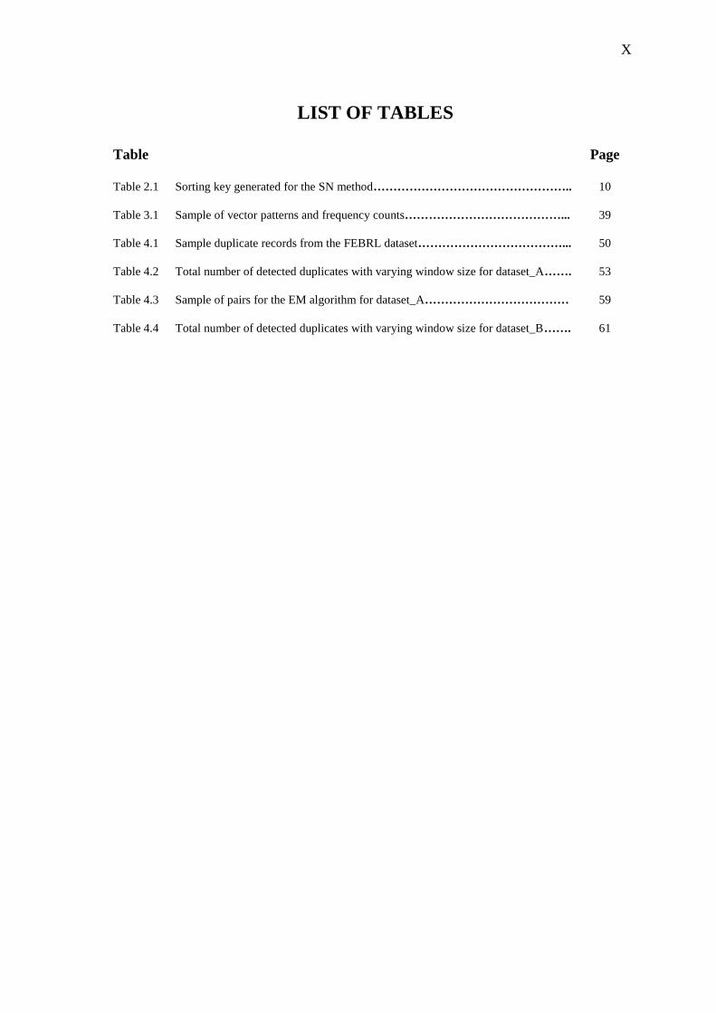
LIST OF TABLES

Table Page

Table 2.1 Sorting key generated for the SN method………………………………………….. 10

Table 3.1 Sample of vector patterns and frequency counts…………………………………... 39

Table 4.1 Sample duplicate records from the FEBRL dataset………………………………... 50

Table 4.2 Total number of detected duplicates with varying window size for dataset_A……. 53

Table 4.3 Sample of pairs for the EM algorithm for dataset_A……………………………… 59

Table 4.4 Total number of detected duplicates with varying window size for dataset_B……. 61

XI

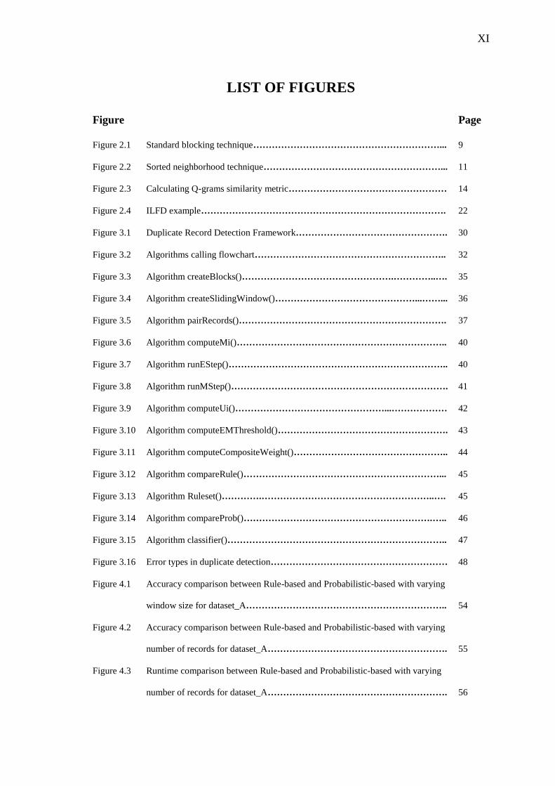
LIST OF FIGURES

Figure Page

Figure 2.1 Standard blocking technique……………………………………………………... 9

Figure 2.2 Sorted neighborhood technique…………………………………………………... 11

Figure 2.3 Calculating Q-grams similarity metric…………………………………………… 14

Figure 2.4 ILFD example……………………………………………………………………. 22

Figure 3.1 Duplicate Record Detection Framework…………………………………………. 30

Figure 3.2 Algorithms calling flowchart…………………………………………………….. 32

Figure 3.3 Algorithm createBlocks()………………………………………….…………..…. 35

Figure 3.4 Algorithm createSlidingWindow()………………………………………...……... 36

Figure 3.5 Algorithm pairRecords()…………………………………………………………. 37

Figure 3.6 Algorithm computeMi()………………………………………………………….. 40

Figure 3.7 Algorithm runEStep()…………………………………………………………….. 40

Figure 3.8 Algorithm runMStep()……………………………………………………………. 41

Figure 3.9 Algorithm computeUi()…………………………………………...……………… 42

Figure 3.10 Algorithm computeEMThreshold()………………………………………………. 43

Figure 3.11 Algorithm computeCompositeWeight()………………………………………….. 44

Figure 3.12 Algorithm compareRule()………………………………………………………... 45

Figure 3.13 Algorithm Ruleset()………….………………………………………………..…. 45

Figure 3.14 Algorithm compareProb()…………………………………………………….….. 46

Figure 3.15 Algorithm classifier()…………………………………………………………….. 47

Figure 3.16 Error types in duplicate detection………………………………………………… 48

Figure 4.1 Accuracy comparison between Rule-based and Probabilistic-based with varying

window size for dataset_A………………………………………………………..

54

Figure 4.2 Accuracy comparison between Rule-based and Probabilistic-based with varying

number of records for dataset_A………………………………………………….

55

Figure 4.3 Runtime comparison between Rule-based and Probabilistic-based with varying

number of records for dataset_A………………………………………………….

56

XII

Figure 4.4 Accuracy comparison between Rule-based and Probabilistic-based technique

with window size=50 and number of records=10,000 for dataset_A…………….

57

Figure 4.5 Accuracy comparison between Rule-based and Probabilistic-based technique

with variation number of passes for dataset_A…………………………………...

58

Figure 4.6 Accuracy comparison between Rule-based and Probabilistic-based techniques

with varying window size for dataset_B………………………………………….

62

Figure 4.7 Accuracy comparison between Rule-based and Probabilistic-based techniques

with varying number of records for dataset_B……………………………………

63

Figure 4.8 Runtime comparison between Rule-based and Probabilistic-based techniques

with varying number of records for dataset_B……………………………………

64

Figure 4.9 Accuracy comparison between Rule-based and Probabilistic-based technique

with window size=50 and number of records=10,000 for dataset_B……………..

65

Figure 4.10 Accuracy comparison between Rule-based and Probabilistic-based technique

with variation number of passes for dataset_B…………………………………...

66

XIII

TABLE OF CONTENTS

PAGE

Dedication……………………………………………………………………………….. V

Acknowledgements……………………………………………………………………… VI

Abstract in English…………………………………………………………………….... VII

Abstract in Arabic.............................................................................................................. IX

List of Tables……………………………………………………………………………. X

List of Figures…………………………………………………………………………… XI

Table of Contents……………………………………………………………………...… XIII

Chapter 1 Introduction………………………………………………………………………..… 1

1.1 Introduction……………………………………………………………………..…… 1

1.2 Records Duplication And Data Quality…………………………………………...… 2

1.3 Detecting Duplicate Records……………………………………………………...… 2

1.4 Motivation…………………………………………………………………………… 4

1.5 Problem Definition………………………………………………………………..… 5

1.6 Contribution………………………………………………………………………… 5

1.7 Thesis Outline…………………………………………………………………….… 6

Chapter 2 Literature Review and Related Studies.…………………………………………… 7

2.1 Comparison Subspace……………………………………………………………..… 7

2.1.1 Standard Blocking Technique…………………………………………… 9

2.1.2 Sorted Neighborhood Technique……………………………………...… 10

2.2 Attribute Matching Techniques…………………………………………………...… 12

2.2.1 Q-Gram Similarity Function…………………………………………..… 12

2.3 Duplicate Records Detection……………………………………………………...… 15

2.3.1 Probabilistic-Based Technique………………………………………...… 15

2.3.1.1 Fellegi-Sunter Model Of Record Linkage…………………… 15

2.3.1.2 EM Algorithm……………………………………………...… 18

2.3.1.3 Alternative Computation Of ui…………………………….… 20

XIV

2.3.1.4 Composite Weights………………………………………...… 21

2.3.2 Rule-Based Technique………………………………………………...… 21

2.4 Related Studies……………........................................................................................ 24

Chapter 3 Duplicate Detection Framework Design and Implementation…………………… 26

3.1 Framework Design………………………………………………………………..… 26

3.2 Technologies………………………………………………………………………… 31

3.3. Implementation Details…………………………………………………………..… 32

Chapter 4 Experimental Evaluation…………………………………………………………… 49

4.1 Data Set……………………………………………………………………………… 49

4.2 Environment………………………………………………………………………… 50

4.3 Experiments…………………………………………………………………………. 50

4.3.1 Experiment Set 1………………….……………………………… 52

4.3.2 Experiment Set 2……………..…………………………………… 60

Chapter 5 Conclusion And Future Work………..…………………………………………..… 68

5.1 Conclusion…..…………………………………………………………………….… 68

5.2 Future Work……………………………………………………………………….… 69

References……………………………………………………………………………………...… 71

Appendices……………………………………………………………………………………..… 73

Appendix 1……………………………………………………………………………… 73

Appendix 2…………………………………………………………………………….… 75

1

Chapter 1

Introduction

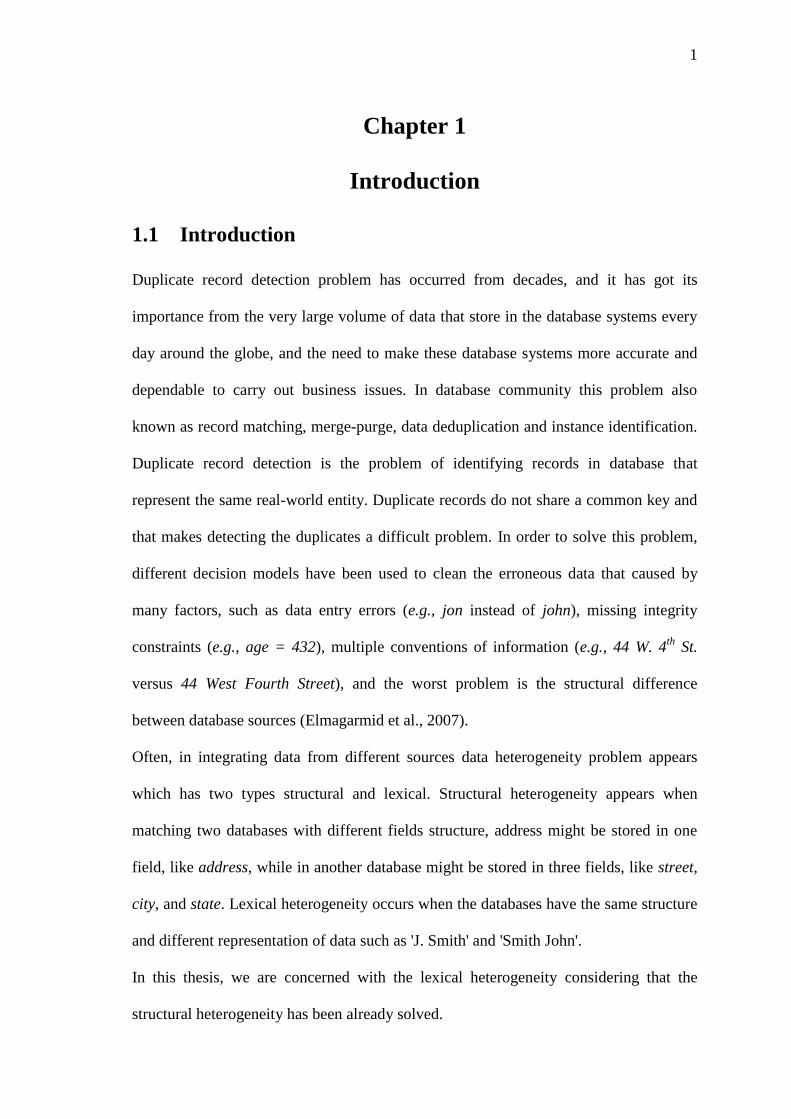
1.1 Introduction

Duplicate record detection problem has occurred from decades, and it has got its

importance from the very large volume of data that store in the database systems every

day around the globe, and the need to make these database systems more accurate and

dependable to carry out business issues. In database community this problem also

known as record matching, merge-purge, data deduplication and instance identification.

Duplicate record detection is the problem of identifying records in database that

represent the same real-world entity. Duplicate records do not share a common key and

that makes detecting the duplicates a difficult problem. In order to solve this problem,

different decision models have been used to clean the erroneous data that caused by

many factors, such as data entry errors (e.g., jon instead of john), missing integrity

constraints (e.g., age = 432), multiple conventions of information (e.g., 44 W. 4th

St.

versus 44 West Fourth Street), and the worst problem is the structural difference

between database sources (Elmagarmid et al., 2007).

Often, in integrating data from different sources data heterogeneity problem appears

which has two types structural and lexical. Structural heterogeneity appears when

matching two databases with different fields structure, address might be stored in one

field, like address, while in another database might be stored in three fields, like street,

city, and state. Lexical heterogeneity occurs when the databases have the same structure

and different representation of data such as 'J. Smith' and 'Smith John'.

In this thesis, we are concerned with the lexical heterogeneity considering that the

structural heterogeneity has been already solved.

2

1.2 Record Duplication and Data Quality

Data quality of a system is essential and important when integrated from different

datasets, so it highly depends on the quality of these resources. Accordingly a false

decision should be avoided. So we need to preprocess datasets to create a complete,

clean, and consistent dataset before any integration tasks (Bleiholder & Naumann,

2008).

Data quality is a very complex concept. The complexity results from its composition of

various characteristics or dimensions, but most researchers have traditionally agreed on

it to be defined as fitness for use. Another definition for data quality is "the distance

between the data views presented by an information system and the same data in the

real world". Such a definition can be seen as an "operational definition", although

evaluating data quality on the basis of comparison with the real world is a very difficult

task (Bertolazzi et al., 2003).

Although, a standard set of dimensions has not been defined yet, researchers agree on

commonly dimensions such as accuracy, completeness, currency, and consistency. The

system which satisfies these dimensions of quality is said to be of high quality

(Scannapieco et al., 2005).

1.3 Detecting Duplicate Records

Currently, duplicate record detection techniques can be classified into two categories:

(Elmagarmid et al., 2007)

Approaches that depend on training data to “learn” how to find the duplicate

records. This category includes (some) probabilistic approaches and supervised

machine learning techniques.

3

Approaches that depend on domain knowledge or on generic distance metrics to

find the duplicate records. This category includes approaches such as Rule-based

and approaches that use declarative languages for matching and approaches that

devise distance metrics appropriate for the duplication detection task.

In this study, two techniques are selected, each from the two approaches. The two

techniques are the Probabilistic-based techniques and the Rule-based technique.

The Probabilistic-based technique is a popular solution that has been used in some of

duplication detection softwares such as FEBRL, TAILOR, and Link King.

Mainly, the Probabilistic-based technique depends on training data to find a maximum

likelihood which helps to determines if a record pair is matching or non-matching.

Moreover, Probabilistic-based method can be used without training data by gaining

benefits of using unsupervised Expectation Maximization (EM) algorithm, in cases of

unavailability of training data, and having a clear structure of datasets.

The EM algorithm makes use of this information to supply the maximum likelihood

estimate.

Winkler (2002) claims that unsupervised EM algorithm works well under these five

conditions:

1. Relatively large percentage of duplicates in the dataset (more than 5%).

2. The class of matching record pairs is well separated from the other classes.

3. The rate of typographical error is low.

4. Sufficient fields to overcome errors in other fields of the record.

5. The conditional independence assumption results in good classification

performance.

On the other hand, the Rule-based technique which also has been used in the Link King

software, has gained much attention because of its potential to result in systems with

4

high accuracy (Elmagarmid et al., 2007). However, the high accuracy could be obtained

basically by the effort and time of an expert to precisely devise good rules. And also it

needs much analysis of the dataset to give the expert a good vision to improve the rules.

Duplicates detection system should include a technique to increase the efficiency of the

system beside of the duplicates detection techniques, particularly when dealing with

large datasets. Such techniques reduce the number of candidate records pairs whilst

maintaining the accuracy of the system. Standard blocking (Baxter et al., 2003), and

sorted neighborhood (Hernández & Stolfo, 1998) techniques apply subspaces creation

using a candidate key created from combination of the dataset attributes to sort the

dataset before applying a block or windows. Choosing the candidate key well is

important in order not to miss detecting a duplicate record.

1.4 Motivation

The important role of database systems and computer networks in various domains of

life has created the need to access and manage information in many distributed systems.

Therefore, there is a need for tools to support systems integration to have an error-free

system with perfect clean data.

The main motivation of this study is the need of finding the best and optimal methods

for detecting the duplicates in systems and to help the users of such systems to automate

the process of duplicate detection so that they don’t need to directly interact and

manually deal with the underlying data.

5

1.5 Problem Definition

Duplicate record detection is an important process in data integration and data cleaning

process. One of the most important stages in this process is the pre-processing stage

where the detection and removal of duplicate records related to the same entity within

one database. Linking or matching records relating to the same entity from several

databases is often required as information from multiple sources which needs to be

integrated, combined or linked in order to enrich data and allow more detailed data

mining analysis. In an error-free system with perfectly clean data, the construction of a

unified view of the data consists of linking or joining two or more records on their key

fields. Unfortunately, data often lack a unique, global identifier that would permit such

an operation.

Accordingly, a large variety of methods have been proposed for detecting approximate

data matching.

Although, researchers try to solve duplicate records problem, it is uncertain which is the

current state-of-the-art, an issue raised by Elmagarmid et. al. (Elmagarmid et al., 2007).

Therefore there is a need to compare the effectiveness of the various methods.

1.6 Contribution

This study contributes in comparing between different decision models that are used for

detecting duplicates in a given dataset. The approach which was suggested for

determining the adequate models for detecting duplicates is used. A framework is

proposed for duplicate record detection that takes its roots from generic designs

suggested and used in solving record linkage and duplicate detection problems. Also,

the performance of the major models used in record matching stage which is the main

part of any duplicate record detection process is evaluated.

6

The contributions we make in this study are:

The researcher introduces some of the most popular techniques that are used in

duplication detection; the major steps in the duplicate detection process are

discussed in brief. The researcher presents the major methods used for matching

records attributes and the strings similarity functions used. The decision models

used in identifying duplicates records are presented and classified.

This study compares between the two main techniques for duplicate record

detection, Rule-based technique and Probabilistic-based technique, and

evaluates their advantages and disadvantages by conducting an experimental

study on synthetic and large-scale benchmarking datasets.

1.7 Thesis Outline

The remainder of this thesis is organized as follows. Chapter 2 reviews the most

important literature related to the duplicate record detection. Chapter 3 describes the

main elements of our framework design and the implementation details for duplicate

record detection problem. Chapter 4 presents the conducted experiments with their used

settings and their results. Finally, the conclusions and future work are presented in

chapter 5.

7

Chapter 2

Literature Review and Related Studies

In this chapter, we present a comprehensive review of the literature on duplicate record

detection.

2. 1 Comparison Subspace

Duplicate record detection depends initially on comparing all records in a database with

each other to find the duplicate records which leads to inefficient duplicate detection

process. For two data sets, A and B, are to be linked, potentially each record from A has

to be compared with all records from B. The total number of potential record pair

comparisons thus equals the product of the size of the two databases, |A|×|B|. With |A|,

|B| denoting the number of records in the data set. For example, linking two databases

with 100,000 records each would result in nearly 1010

record pair comparisons. With the

expensive detailed comparing of the fields, and the fact that the number of duplicate

record is small, this will consume much time and resources. In addition, there is no

unique key in the database to be linked. Meanwhile, the efficiency is a major challenge

to hold especially in large database. So the convenient solution is to reduce the number

of comparisons by using techniques that group dataset into blocks or clusters using

Blocking Key Value (BKV) with respect to a defined criterion or some threshold values

(Christen & Churches, 2005) (Christen, 2007).

With having the unique key and splitting dataset into blocks, candidate pairs could be

generated from the same block. That will certainly improve the efficiency with

attention to reducing the quality of duplicate record detection (Tamilselvi & Saravanan,

2009).

The blocking process can be split into the following two steps: (Christen, 2007)

8

1- Build: All records from the data set are read, the blocking key values are created

from record attributes, and the records are inserted into an index data structure. For

most blocking methods, a basic inverted index can be used. The blocking key

values will become the keys of the inverted index, and the record identifiers of all

records that have the same blocking key value will be inserted into the same

inverted index list.

2- Retrieve: Record identifiers are retrieved from the index data structure block by

block, and candidate record pairs are generated. Each record in a block will be

paired with all other records in the same block. The generated candidate record

pairs are then compared and the resulting vectors containing the numerical

comparison values are given to a classifier.

We should note that the choice of blocking keys is usually done manually by domain

and duplication detection experts and are usually chosen to be very general in order to

produce a high quality result, while also producing a reasonable reduction in the amount

of data required to compare against for each record to be matched.

A blocking key can be defined as either the values taken from a single record attribute

(or parts of values, like the first two initial letters only), or the concatenation of values

(or parts of them) from several attributes. (Christen, 2007)

Next we present some of the major blocking methods that are used to improve the

efficiency and scalability of duplicate detection process.

9

2.1.1 Standard Blocking Technique

The Standard Blocking technique group records into disjoint blocks where they have the

same BKV, and then compare all pairs of records only within the same block. A

blocking key is defined to be composed from the record attributes of the data set.

Assuming duplicate detection applied on a data set with N records, and the blocking

technique given B number of blocks (all of the same size containing N/B records), the

resulting number of record pair comparisons is O (N2/B). Thus, the overall number of

comparisons is greatly reduced. (Baxter et al., 2003)

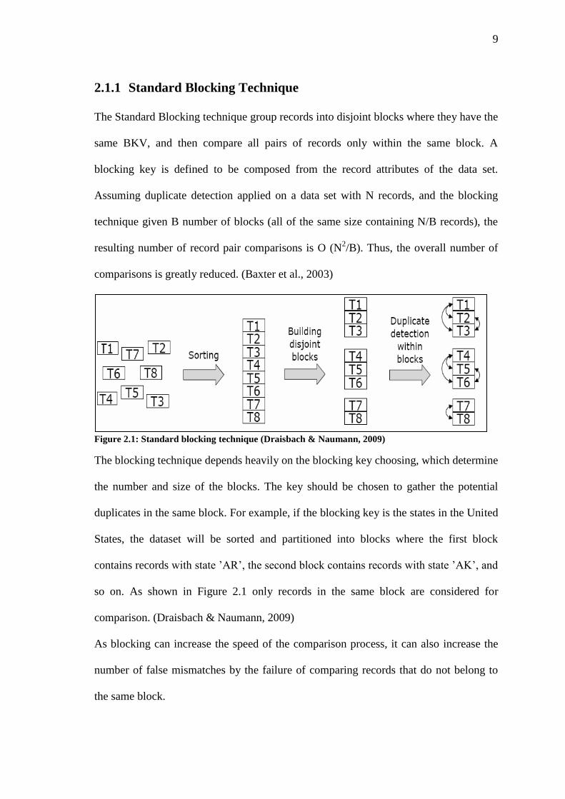
Figure 2.1: Standard blocking technique (Draisbach & Naumann, 2009)

The blocking technique depends heavily on the blocking key choosing, which determine

the number and size of the blocks. The key should be chosen to gather the potential

duplicates in the same block. For example, if the blocking key is the states in the United

States, the dataset will be sorted and partitioned into blocks where the first block

contains records with state ’AR’, the second block contains records with state ’AK’, and

so on. As shown in Figure 2.1 only records in the same block are considered for

comparison. (Draisbach & Naumann, 2009)

As blocking can increase the speed of the comparison process, it can also increase the

number of false mismatches by the failure of comparing records that do not belong to

the same block.

10

2.1.2 Sorted Neighborhood Technique

Hernández and Stolfo proposed a technique called Sorted Neighborhood (SN) or

Windowing to reduce the number of comparisons by limiting the similarity measures on

a small portion of the dataset. The SN technique consists of the following three steps:

(Hernández & Stolfo, 1998)

1- Create key: A blocking key for each record in the data set is computed by

extracting relevant attributes, or a sequence of substrings within the attributes,

chosen from the record in an ad hoc manner. Attributes that appear first in the

key have a higher priority than those that appear subsequently. For example, the

key may composed from first three constants characters of a person surname

concatenated by the first three constants characters of a person given name and

first three digits of the social security id as shown in Table 2.1.

2- Sort data: The records in the data set are sorted by using the blocking key value

created in the first step.

3- Merge: A window of fixed size w >1 is moved through the sequential list of

records in order to limit the Comparisons for matching records to those records

in the window. If the size of the window is w records, then every new record

that enters that window is compared with the previous w - 1 record to find

“matching” records. The first record in the window slides out of it as shown in

Figure 2.2.

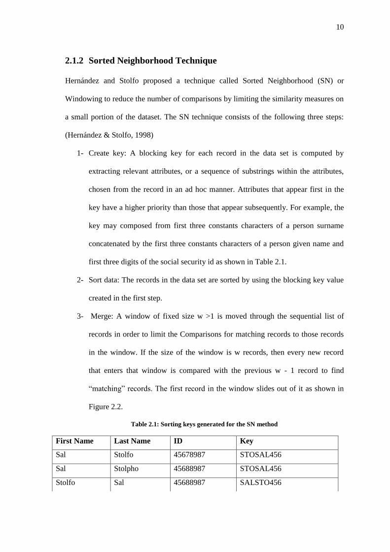
Table 2.1: Sorting keys generated for the SN method

First Name Last Name ID Key

Sal Stolfo 45678987 STOSAL456

Sal Stolpho 45688987 STOSAL456

Stolfo Sal 45688987 SALSTO456

11

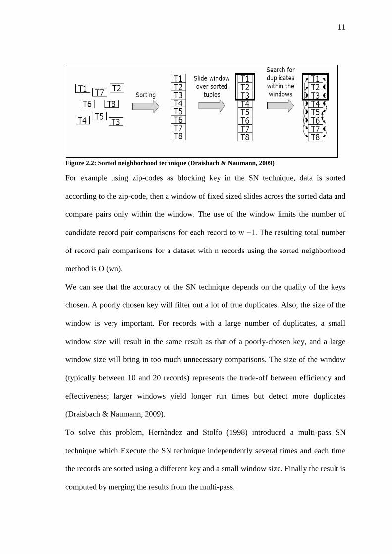
Figure 2.2: Sorted neighborhood technique (Draisbach & Naumann, 2009)

For example using zip-codes as blocking key in the SN technique, data is sorted

according to the zip-code, then a window of fixed sized slides across the sorted data and

compare pairs only within the window. The use of the window limits the number of

candidate record pair comparisons for each record to w −1. The resulting total number

of record pair comparisons for a dataset with n records using the sorted neighborhood

method is O (wn).

We can see that the accuracy of the SN technique depends on the quality of the keys

chosen. A poorly chosen key will filter out a lot of true duplicates. Also, the size of the

window is very important. For records with a large number of duplicates, a small

window size will result in the same result as that of a poorly-chosen key, and a large

window size will bring in too much unnecessary comparisons. The size of the window

(typically between 10 and 20 records) represents the trade-off between efficiency and

effectiveness; larger windows yield longer run times but detect more duplicates

(Draisbach & Naumann, 2009).

To solve this problem, Hernàndez and Stolfo (1998) introduced a multi-pass SN

technique which Execute the SN technique independently several times and each time

the records are sorted using a different key and a small window size. Finally the result is

computed by merging the results from the multi-pass.

12

2. 2 Attribute Matching Techniques

Duplicate record detection depends substantially on string comparison techniques to

determine if two records are matching or non-matching. It is axiomatic to find the

similarity between two strings instead of equality because it is common that mismatches

happen due to typographical error. Various string similarity techniques have been

created. In this study one of them is used, we briefly discuss it.

2.2.1 Q-Gram Similarity Function

A Q-gram could be defined as short substrings of length q from a given string. The

substrings could be phonemes, syllables, letters, or words according to the usage of Q-

gram function. Q-gram has many types according to the length of the substrings such as

unigram with size of one, bigram with size of two, trigram with size of three, and size

four or more is simply called a Q-gram. Letter Q-grams, including trigrams, bigrams,

and/or unigrams, have been used in a variety of ways in text recognition and spelling

correction (Innerhofer-Oberperfler, 2004).

The notion of Q-grams for a given string , its Q-grams are obtained by “sliding” a

window of length q over the characters of . Since Q-grams at the beginning and the

end of the string can have fewer than q characters from we introduce new characters

“#” and “%” not in , and conceptually extend the string by prefixing or padding it

with q – 1 occurrences of “#” and suffixing it with q -1 occurrences of “%”. Thus, each

Q-gram contains exactly q characters, though some of these may not be from the

alphabet .

The intuition behind the use of Q-grams as a foundation for approximate string

processing is that when two strings 1 and 2 are within a small edit distance of each

other, they share a large number of Q-grams in common (Ukkonen, 1992).

13

For example consider the Q-grams of length q=3 for string “john smith” are { (##j),

(#jo), (joh), ( ohn), ( hn_), ( n_s), ( _sm), ( smi), ( mit), ( ith), ( th%), ( h%%) }.

Similarly, the Qgrams of length q=3 for “john a smith”, which is at an edit distance of

two from “john smith”, are { ( ##j), ( #jo), ( joh), ( ohn), ( hn_), ( n_a), ( _a_), ( a_s), (

_sm), ( smi),( mit), ( ith), ( th%), ( h%%) }.

If we ignore the position information, the two Q-gram sets have 11 Q-grams in

common. Interestingly, only the first five Q-grams of the first string are also Q-grams of

the second string.

The Q-grams similarity metric between two strings is constructed ranging from 0 to 1.0

using a normalized formula,

(2.1)

Where |Gs1Gs2| is the number of common Q-grams between S1 & S2, |Gs1| and |Gs2| is

the number of Q-grams of s1 and s2 respectively.

For the above example, we have |Gs1|=12, |Gs2|=14, |Gs1Gs2|=11, so the similarity

between them is 0.8511 according to the above formula.

Also consider a Q-grams of length q = 3 for S1 = ’Street’ can be constructed as Gs1=

{##S, #St, Str, tre, ree, eet, et#, t##}, and S2 = ’Steret’, are Gs2 = {##S, #St, Ste, ter, ere,

ret, et#, t##}. The two strings have four Q-grams in common. We have |Gs1|=8, |Gs2|=8,

|Gs1Gs2|=4, so the similarity between them is 0.5 according to the above formula.

Figure 2.3 shows the calculation of the similarity metric between two different strings

S1 and S2 (Innerhofer-Oberperfler, 2004).

14

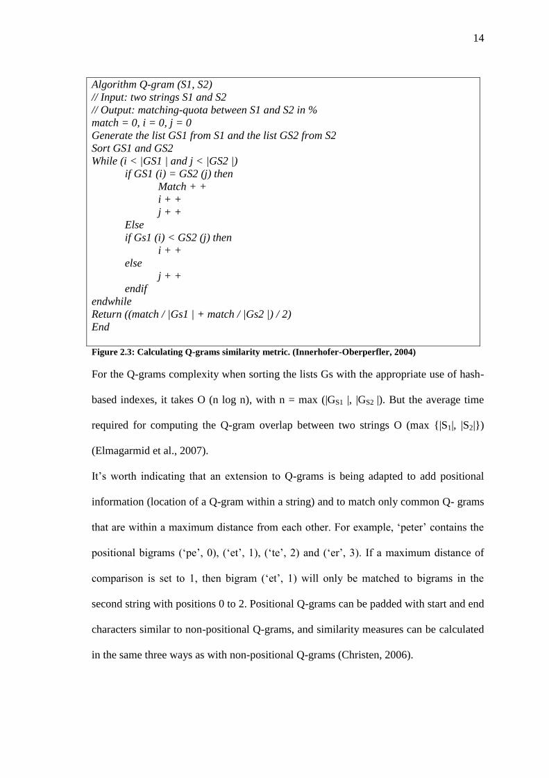
Algorithm Q-gram (S1, S2)

// Input: two strings S1 and S2

// Output: matching-quota between S1 and S2 in %

match = 0, i = 0, j = 0

Generate the list GS1 from S1 and the list GS2 from S2

Sort GS1 and GS2

While (i < |GS1 | and j < |GS2 |)

if GS1 (i) = GS2 (j) then

Match + +

i + +

j + +

Else

if Gs1 (i) < GS2 (j) then

i + +

else

j + +

endif

endwhile

Return ((match / |Gs1 | + match / |Gs2 |) / 2)

End

Figure 2.3: Calculating Q-grams similarity metric. (Innerhofer-Oberperfler, 2004)

For the Q-grams complexity when sorting the lists Gs with the appropriate use of hash-

based indexes, it takes O (n log n), with n = max (|GS1 |, |GS2 |). But the average time

required for computing the Q-gram overlap between two strings O (max {|S1|, |S2|})

(Elmagarmid et al., 2007).

It’s worth indicating that an extension to Q-grams is being adapted to add positional

information (location of a Q-gram within a string) and to match only common Q- grams

that are within a maximum distance from each other. For example, ‘peter’ contains the

positional bigrams (‘pe’, 0), (‘et’, 1), (‘te’, 2) and (‘er’, 3). If a maximum distance of

comparison is set to 1, then bigram (‘et’, 1) will only be matched to bigrams in the

second string with positions 0 to 2. Positional Q-grams can be padded with start and end

characters similar to non-positional Q-grams, and similarity measures can be calculated

in the same three ways as with non-positional Q-grams (Christen, 2006).

15

2. 3 Duplicate Records Detection

So far, we have described techniques that can be used to match individual fields of a

record. In most real-life situations, however, the records consist of multiple fields;

making the duplicate detection problem much more complicated and a decision must be

made as to whether consider these records as matching, or non-matching (Wang, 2008).

Many techniques may be used for matching records with multiple fields. The presented

methods can be broadly divided into two categories: (Elmagarmid et al., 2007)

Approaches that rely on training the data to “learn” how to match the records.

This category includes (some) probabilistic approaches and supervised machine

learning models.

Approaches that rely on domain knowledge or on generic distance metrics to

match records. This category includes approaches that use declarative languages

for matching and approaches that devise distance metrics.

2.3.1 Probabilistic-Based Technique

In this study we implement the Probabilistic-based technique using the Fellegi-Sunter

model of record linkage without training data instead we use the Expectation

Maximization (EM) algorithm to compute the maximum likelihood estimates.

2.3.1.1 Fellegi-Sunter Model of Record Linkage

Newcombe et al. (1959) ideas in duplicate detection were formalized as a mathematical

model by Fellegi and Sunter (1969). Given record pair as input to the decision model,

record pair is classified as matching or non-matching whose density function is different

for each of the two classes. We used the same notation provided by Fellegi and Sunter.

We represent the set of ordered record pairs (with a record drawn from each file A and

B for each pair) as

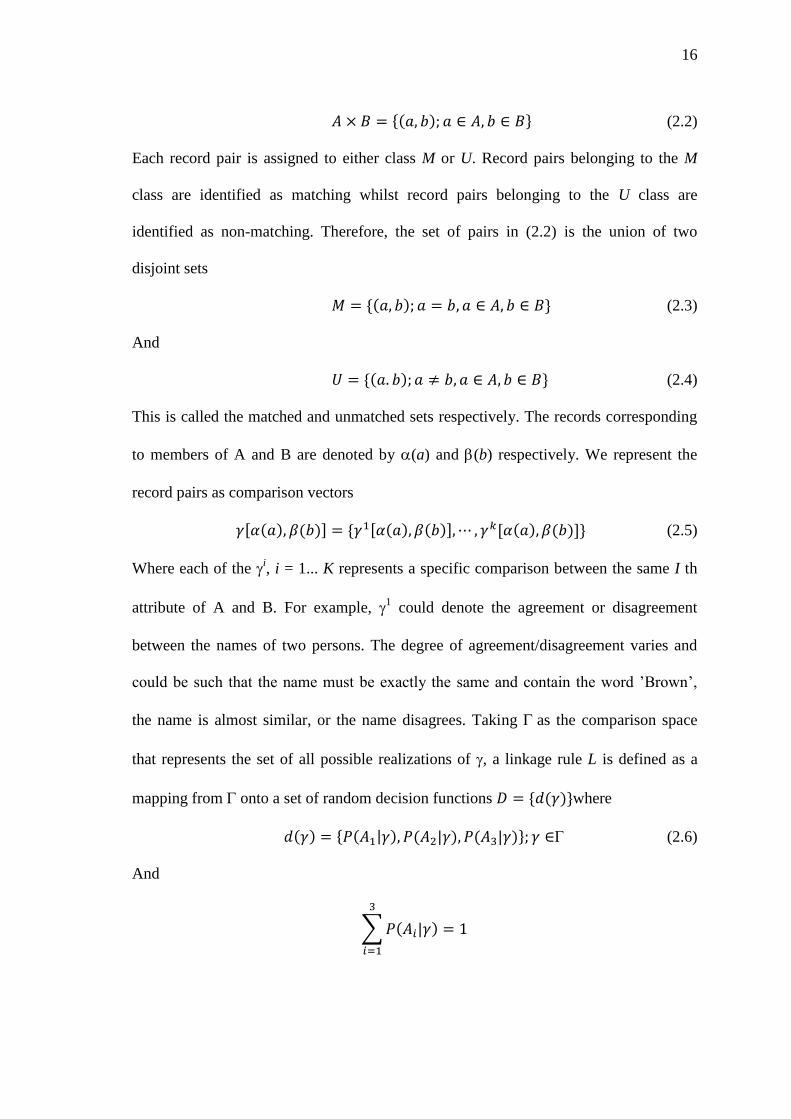
16

(2.2)

Each record pair is assigned to either class M or U. Record pairs belonging to the M

class are identified as matching whilst record pairs belonging to the U class are

identified as non-matching. Therefore, the set of pairs in (2.2) is the union of two

disjoint sets

(2.3)

And

(2.4)

This is called the matched and unmatched sets respectively. The records corresponding

to members of A and B are denoted by (a) and (b) respectively. We represent the

record pairs as comparison vectors

(2.5)

Where each of the i, i = 1... K represents a specific comparison between the same I th

attribute of A and B. For example, 1 could denote the agreement or disagreement

between the names of two persons. The degree of agreement/disagreement varies and

could be such that the name must be exactly the same and contain the word ’Brown’,

the name is almost similar, or the name disagrees. Taking as the comparison space

that represents the set of all possible realizations of , a linkage rule L is defined as a

mapping from onto a set of random decision functions where

Γ (2.6)

And

17

The three decisions are denoted as link (A1), non-link (A3), and possible link (A2). The

possible link class is introduced for ambiguous cases such as insufficient information.

Rather than falsely classifying the record pair that falls under these cases as not linked,

it is safer to classify it as a possible match for further examination. A record pair is

considered linked if the probability that it is a link, is greater than

the probability that it is a non-link, . To solve this, we follow the

Bayes decision rule for minimum error which introduces a likelihood ratio based on

conditional probabilities of the record pair when it is known to be a link or non-link.

These values can be computed using a training set of pre-labeled record pairs or using

the EM algorithm.

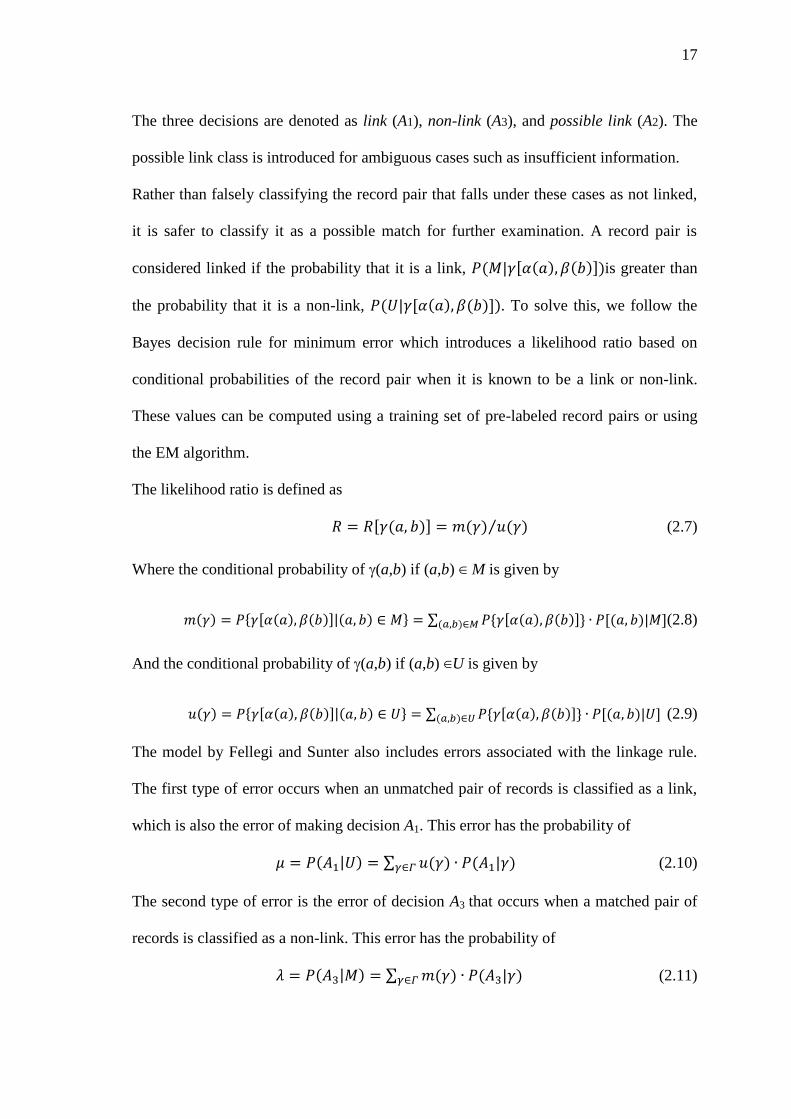
The likelihood ratio is defined as

(2.7)

Where the conditional probability of (a,b) if (a,b) ∈ M is given by

(2.8)

And the conditional probability of (a,b) if (a,b) ∈U is given by

(2.9)

The model by Fellegi and Sunter also includes errors associated with the linkage rule.

The first type of error occurs when an unmatched pair of records is classified as a link,

which is also the error of making decision A1. This error has the probability of

(2.10)

The second type of error is the error of decision A3 that occurs when a matched pair of

records is classified as a non-link. This error has the probability of

(2.11)

18

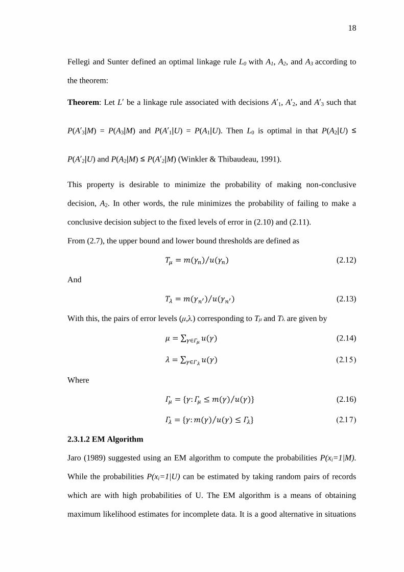
Fellegi and Sunter defined an optimal linkage rule L0 with A1, A2, and A3 according to

the theorem:

Theorem: Let L′ be a linkage rule associated with decisions A′1, A′2, and A′3 such that

P(A′3|M) = P(A3|M) and P(A′1|U) = P(A1|U). Then L0 is optimal in that P(A2|U) ≤

P(A′2|U) and P(A2|M) ≤ P(A′2|M) (Winkler & Thibaudeau, 1991).

This property is desirable to minimize the probability of making non-conclusive

decision, A2. In other words, the rule minimizes the probability of failing to make a

conclusive decision subject to the fixed levels of error in (2.10) and (2.11).

From (2.7), the upper bound and lower bound thresholds are defined as

(2.12)

And

(2.13)

With this, the pairs of error levels (μ,) corresponding to Tμ and Tare given by

(2.14)

Where

(2.16)

2.3.1.2 EM Algorithm

Jaro (1989) suggested using an EM algorithm to compute the probabilities P(xi=1|M).

While the probabilities P(xi=1|U) can be estimated by taking random pairs of records

which are with high probabilities of U. The EM algorithm is a means of obtaining

maximum likelihood estimates for incomplete data. It is a good alternative in situations

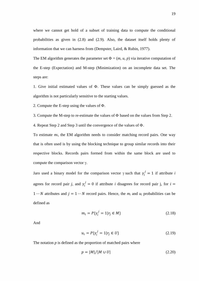
19

where we cannot get hold of a subset of training data to compute the conditional

probabilities as given in (2.8) and (2.9). Also, the dataset itself holds plenty of

information that we can harness from (Dempster, Laird, & Rubin, 1977).

The EM algorithm generates the parameter set = (m, u, p) via iterative computation of

the E-step (Expectation) and M-step (Minimization) on an incomplete data set. The

steps are:

1. Give initial estimated values of . These values can be simply guessed as the

algorithm is not particularly sensitive to the starting values.

2. Compute the E-step using the values of .

3. Compute the M-step to re-estimate the values of based on the values from Step 2.

4. Repeat Step 2 and Step 3 until the convergence of the values of .

To estimate mi, the EM algorithm needs to consider matching record pairs. One way

that is often used is by using the blocking technique to group similar records into their

respective blocks. Records pairs formed from within the same block are used to

compute the comparison vector .

Jaro used a binary model for the comparison vector such that if attribute i

agrees for record pair j, and if attribute i disagrees for record pair j, for

attributes and record pairs. Hence, the mi and ui probabilities can be

defined as

(2.18)

And

(2.19)

The notation p is defined as the proportion of matched pairs where

(2.20)

20

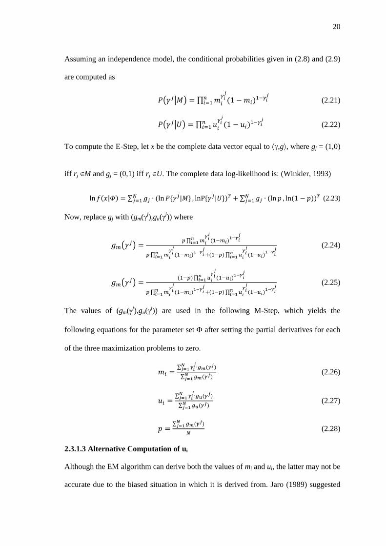
Assuming an independence model, the conditional probabilities given in (2.8) and (2.9)

are computed as

(2.21)

(2.22)

To compute the E-Step, let x be the complete data vector equal to ,g⟩, where gj = (1,0)

iff rj ∈M and gj = (0,1) iff rj ∈U. The complete data log-likelihood is: (Winkler, 1993)

(2.23)

Now, replace gj with (gm(j),gu(

j)) where

(2.24)

(2.25)

The values of (gm(j),gu(

j)) are used in the following M-Step, which yields the

following equations for the parameter set after setting the partial derivatives for each

of the three maximization problems to zero.

(2.26)

(2.27)

(2.28)

2.3.1.3 Alternative Computation of ui

Although the EM algorithm can derive both the values of mi and ui, the latter may not be

accurate due to the biased situation in which it is derived from. Jaro (1989) suggested

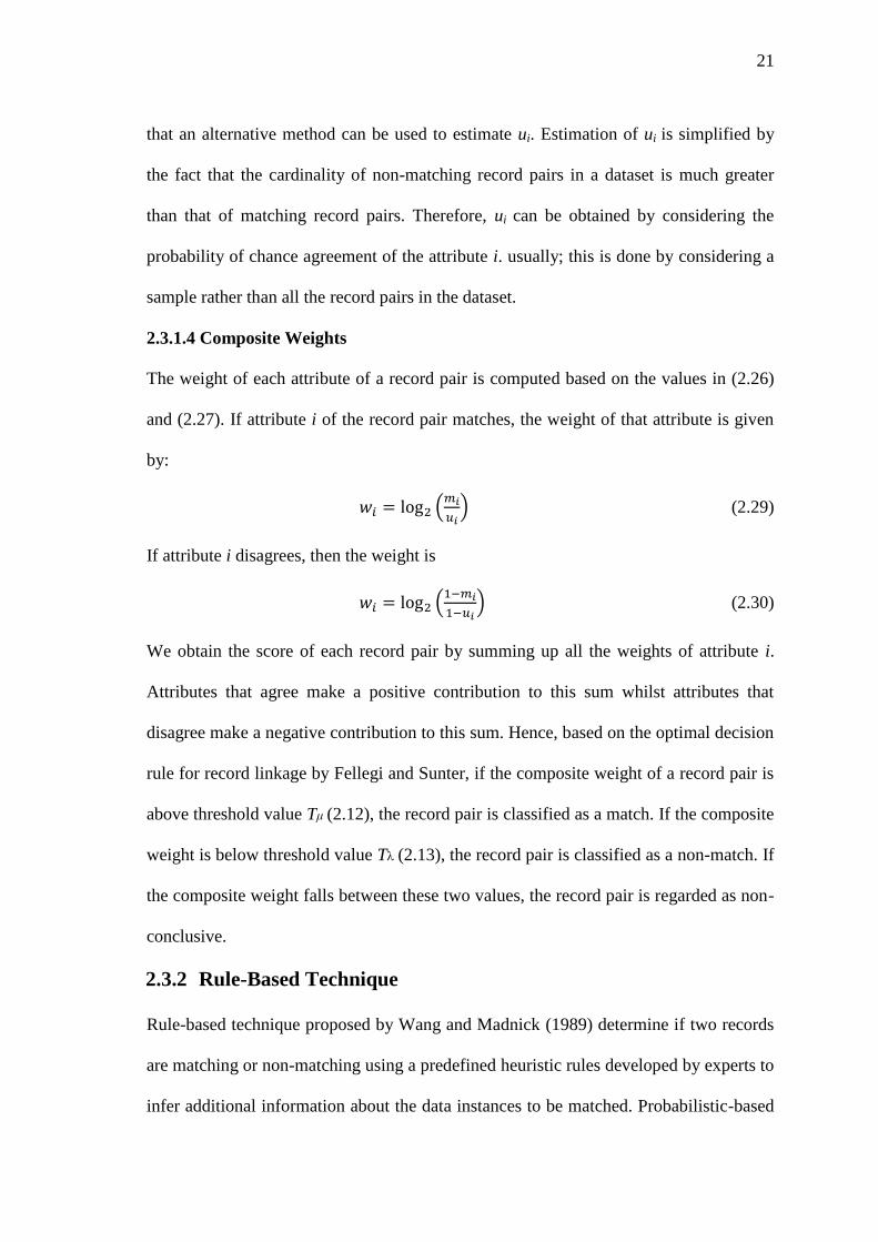
21

that an alternative method can be used to estimate ui. Estimation of ui is simplified by

the fact that the cardinality of non-matching record pairs in a dataset is much greater

than that of matching record pairs. Therefore, ui can be obtained by considering the

probability of chance agreement of the attribute i. usually; this is done by considering a

sample rather than all the record pairs in the dataset.

2.3.1.4 Composite Weights

The weight of each attribute of a record pair is computed based on the values in (2.26)

and (2.27). If attribute i of the record pair matches, the weight of that attribute is given

by:

(2.29)

If attribute i disagrees, then the weight is

(2.30)

We obtain the score of each record pair by summing up all the weights of attribute i.

Attributes that agree make a positive contribution to this sum whilst attributes that

disagree make a negative contribution to this sum. Hence, based on the optimal decision

rule for record linkage by Fellegi and Sunter, if the composite weight of a record pair is

above threshold value Tμ (2.12), the record pair is classified as a match. If the composite

weight is below threshold value T(2.13), the record pair is classified as a non-match. If

the composite weight falls between these two values, the record pair is regarded as non-

conclusive.

2.3.2 Rule-Based Technique

Rule-based technique proposed by Wang and Madnick (1989) determine if two records

are matching or non-matching using a predefined heuristic rules developed by experts to

infer additional information about the data instances to be matched. Probabilistic-based

22

technique assign a weight for each attribute whilst Rule-based technique each attribute

is given a weight of one or zero. For example, an expert might define rules such as:

IF age < 22

THEN status = undergraduate

ELSE status = graduate

IF course_id = 564 AND course_id = 579

THEN student_major = MIS

Such rules are used to cluster records that represent the same real-world entity.

However, since the rules are heuristically derived, the output from these rules may not

be correct (Wang & Madnick, 1989).

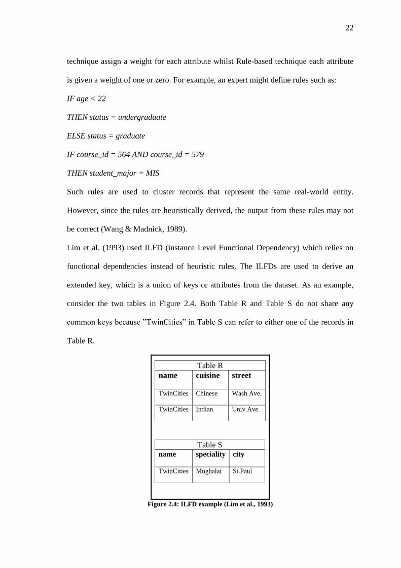
Lim et al. (1993) used ILFD (instance Level Functional Dependency) which relies on

functional dependencies instead of heuristic rules. The ILFDs are used to derive an

extended key, which is a union of keys or attributes from the dataset. As an example,

consider the two tables in Figure 2.4. Both Table R and Table S do not share any

common keys because ”TwinCities” in Table S can refer to either one of the records in

Table R.

Table R

name cuisine street

TwinCities Chinese Wash.Ave.

TwinCities Indian Univ.Ave.

Table S

name speciality city

TwinCities Mughalai St.Paul

Figure 2.4: ILFD example (Lim et al., 1993)

23

To solve this, we can assert in the following IFLD that the values of attribute speciality

can infer the values of attribute cuisine. Hence, Table R and Table S can be matched

using the extended key (name, cuisine) and the corresponding extended key equivalence

rule, which states that two records are similar when their name and cuisine values are

the same.

ILFD:

(e2.speciality = Mughalai) -> (e2.cuisine = Indian)

Extended Key Equivalence Rule:

(e1.name = e2.name) AND (e1.cuisine = e2.cuisine) -> (e1 and e2 are the same)

Hernàndez and Stolfo suggest the use of an equational theory that dictates the logic of

domain equivalence. For example, the following is a rule that exemplifies one axiom of

the equational theory developed for an employee database: (Hernàndez & Stolfo, 1998)

Given two records, r1 and r2

IF the last name of r1 equals the last name of r2,

AND the first names differ slightly,

AND the address of r1 equals the address of r2

THEN

r1 is equivalent to r2

The implementation of differ slightly of the first names based upon the distance-based

technique to determine the typographical gap. The gap is then compared with a

predefined threshold which is normally obtained through experimental evaluation to

decide if the two records are matching or non-matching. A poor choice of threshold

value would result in false positives or false negatives. For instance, if the threshold

value is high, we would have missed a number of duplicates. On the other hand,

relaxing the value of threshold also means that non-duplicates would be misclassified as

24

matching records. Therefore, a good matching declarative rule very much depends on

the selection of distance functions and a proper threshold.

2.4 Related Studies

Lots of work and researches in the field of duplicate record detection have been

proposed and many systems have been implemented with different approaches to detect

duplicate record. In this section we are going to introduce some of the most important

related studies in this field which provides us a good guidance to our work.

(Hernández & Stolfo, 1998): The authors introduced a system for accomplishing

data cleansing tasks and demonstrate its use for cleansing lists of names of

potential customers in a direct marketing-type application. The system provides

a rule programming module using an intelligent equational theory in addition to

the sorted neighborhood method as a blocking method.

(Gu et al., 2003): The authors presented the current standard practices in record

linkage methodology. The definition of the record linkage problem, the formal

probabilistic model and an outline of the standard practice algorithms and its

recent proposals. And it concludes with a summary of the current methods and

the most worthwhile research directions.

(Christen 2007): The author evaluated the traditional, as well as several recently

developed, blocking methods within a common framework with regard to the

quality of the candidate record pairs generated by them. Also proposed

modifications to existing blocking methods that replace the traditional global

thresholds with nearest-neighbor based parameters.

(Elmagarmid et al., 2007): The authors presented a thorough analysis of the

literature on duplicate record detection covering similarity metrics that are

25

commonly used to detect similar field entries. They also present an extensive set

of duplicate detection techniques that can detect approximately duplicate records

in a database. They also cover multiple methods for improving the efficiency

and scalability of approximate duplicate detection algorithms. In addition to

coverage of existing software tools with a brief discussion of the big open

problems in this filed.

(Draisbach & Naumann, 2009): The authors in this paper briefly introduced and

analyzed two popular families of methods for duplicate detection. Blocking

methods and Windowing methods. Also the authors proposed a generalized

algorithm, the Sorted Blocks method and compared the approaches qualitatively

and experimentally.

(Tamilselvi & Saravanan, 2009): The authors present a general sequential

framework for duplicate detection and elimination using a rule-based approach

to identify exact and inexact duplicates and to eliminate duplicates. The

proposed framework uses six steps to improve the process of duplicate detection

and elimination. Also the authors compare this new framework with previous

approaches using the token concept in order to speed up the data cleaning

process and reduce its complexity. Analysis of several blocking key is made to

select best blocking key to bring similar records together through extensive

experiments to avoid comparing all pairs of records.

26

Chapter 3

Duplicate Detection Framework Design and

Implementation

3.1 Framework Design

Our framework design for duplicate record detection is derived from the generic record

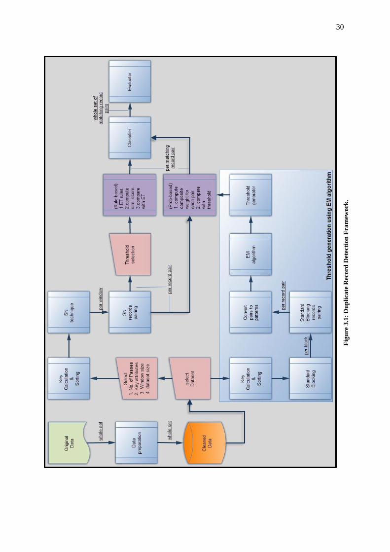
linkage framework suggested by (Gu et al., 2003). Figure 3.1, clarifies the framework

that has developed for our duplicate record detection system. The stages on this

framework are as following:

Database: the MySQL database contains dataset A and dataset B. For each dataset

that is evaluated; the entire dataset is queried and loaded into memory after the

preparation stage.

Data preparation: this stage refers to the process in which our datasets would be

processed and stored in a uniform manner in the database.

User interaction: in this stage, user would interact with the system through the user

interface for the selection of dataset, and selection of the attributes to be used as a key

for the SN technique for each pass of the three passes that we use with the SN

technique. And supply the parameters required for the duplicate detection techniques.

Such as, dataset size, window size, and threshold value for the Rule-based technique.

Then user chooses the decision model.

Blocking keys generator: the blocking keys are generated from the selected

attributes of each record, and then the data are sorted according to these keys. For the

27

SN technique we use three passes so there are three keys (one for each pass). And for

the standard blocking technique one key is generated.

Records blocking: to reduce the comparison space, a blocking technique is used to

group the data into blocks. Two blocking techniques are used in this system.

Standard blocking technique: dataset is divided into non-overlapping blocks; all the

records in the same block have the same key value, and then records are passed to the

pairing stage. We use this technique just to compute the EM algorithm.

Sorted-Neighborhood technique: after sorting the dataset according the key it is

divided into overlapping windows with window size defined by the user, then records

are passed to the pairing stage to be used by the selected decision model.

Records pairing: in this stage, records from each block are paired together and sent

to the EM algorithm to computes the threshold value. Meanwhile, records from each

window are paired together and sent to be tested by the chosen decision model pair by

pair. Of course the pairing in the blocks is different from the paring in the windows.

Threshold generator for Probabilistic-based technique: using the EM

algorithm the threshold value is computed to be used by the Probabilistic-based

technique. Estimating the threshold value could be done by computes the comparison

vector for each record pair that received from the standard block technique. All

comparison vectors and there frequency counts are sent to the EM algorithm to estimate

mi and ui. These two values used to compute the threshold value.

Decision models matcher: the matching stage consists of a Rule-based matcher

that employs the Rule-based technique, and the Probabilistic-based matcher that

employs the Probabilistic-based technique. In this stage the decision is made if the

record pair is matched or non-matched.

28

Rule-based matcher: after receiving a record pairs paired up from sliding window, the

Rule-based matcher computes the similarity scores for each attribute in the record pair.

The scores are sent to the Equational Theory rules to check if they satisfy the threshold.

If they do, the record pair is considered matching and is sent to be classified.

Probabilistic-based matcher: to determine if a record pair is matching or non-

matching, we used the sliding window to obtain record pairs that passed to the

Probabilistic-based matcher to compute the composite weight of the record pair. The

composite weight is compared with the threshold value that generated by the EM

algorithm. If the composite weight is above the threshold value, the record pair is

considered matched and sent to the classifier.

Classifier: the classifier does the following:

1. Determine the record pairs that should grouped together on the fact that all

records in the same group are duplicates for each other.

2. Make sure not to overlap between the groups after next matching process.

3. Compute transitive closure over several independent runs (multi-passes).

Evaluator: the successful measuring of the duplication detection is an important but

hard task, because of the lake of the gold standard for the dataset. Privacy and

confidentially are the main difficulties preventing having a benchmark dataset. We

described the duplication detection measures that have been used to evaluate the

performance of our duplication detection techniques such as Recall, Precision, F-Score,

and Time complexity (Naumann & Herschel, 2010).

Recall (true positive rate)

29

Recall also known as sensitivity, measures the ratio of correctly identified duplicates

compared to all true duplicates. And it used commonly in epidemiological studies.

Recall estimated using the formula:

Recall =

=

(4.1)

Precision

It is also called a positive predictor value that measures the ratio of correctly identified

duplicates compared to all declared duplicates. In the information retrieval field

precision is widely used in combination with the recall measure for visualization in

precision-recall graph. Precision estimated using the formula:

Precision =

=

(4.2)

F-Score

Both recall and precision measures should be maximized, but there is a tradeoff

between them. F-score measure captures this tradeoff by combining recall and precision

via a harmonic mean. So it’s a measure of accuracy of the experiment (Yan et al.,

2007). The F-score is given by:

F-Score=

(4.3)

Time complexity, which measures how well the system scales in terms of time.

30

Fig

ure

3.1

: D

up

lica

te R

eco

rd D

ete

cti

on

Fra

mew

ork

.

31

3.2 Technologies

In evaluating and comparing the two duplication detection techniques, it has been used

the following technologies:

Java Development Kit (JDK): the core of the system is built using the Java

Platform (Standard Edition 6). Java is chosen because of its cross-platform capabilities.

MySQL server 6.0 database environment: MySQL is the world’s most

popular open source database, as quoted from its website Due to its free usage and fast

performance; it is favored as the relational database management system (RDBMS) of

choice for this project.

Netbeans: the development environment used was Netbeans IDE 7.0.1 for compiling

and executions.

MySQL connector Java: the MySQL Connector Java provides the functionality to

access the database system from within the Java program. It provides functionalities to

access and retrieves data from the database. The MySQL Connector Java driver is

downloadable from the MySQL website. The version of the connector used for this

project is 5.1.18.

SimMetrics: SimMetrics is an open source Java library of distance metrics. It

contains programs for a variety of edit distance and token-based metrics such as Smith-

Waterman, Jaro, Needleman-Wunsch, Jaccard, TFIDF, Levenstein, and Q-Gram

distance. It takes in a pair of string data and return the distance result in the form of

floating-point based number (0.0 - 1.0).

32

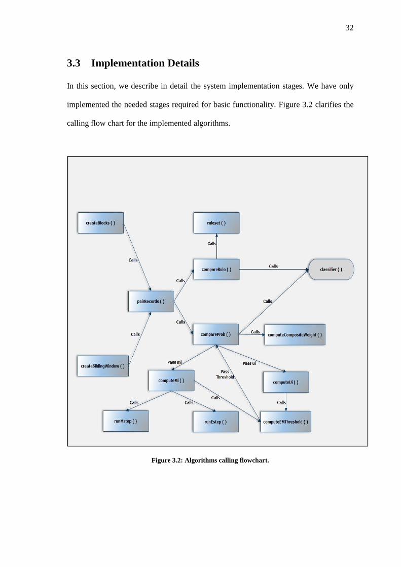
3.3 Implementation Details

In this section, we describe in detail the system implementation stages. We have only

implemented the needed stages required for basic functionality. Figure 3.2 clarifies the

calling flow chart for the implemented algorithms.

Figure 3.2: Algorithms calling flowchart.

33

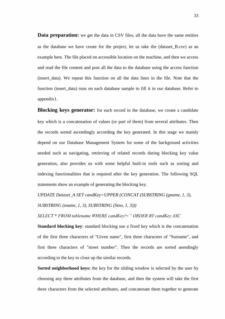
Data preparation: we get the data in CSV files, all the data have the same entities

as the database we have create for the project, let us take the (dataset_B.csv) as an

example here. The file placed on accessible location on the machine, and then we access

and read the file content and post all the data to the database using the access function

(insert_data). We repeat this function on all the data lines in the file. Note that the

function (insert_data) runs on each database sample to fill it in our database. Refer to

appendix1.

Blocking keys generator: for each record in the database, we create a candidate

key which is a concatenation of values (or part of them) from several attributes. Then

the records sorted ascendingly according the key generated. In this stage we mainly

depend on our Database Management System for some of the background activities

needed such as navigating, retrieving of related records during blocking key value

generation, also provides us with some helpful built-in tools such as sorting and

indexing functionalities that is required after the key generation. The following SQL

statements show an example of generating the blocking key.

UPDATE Dataset_A SET candKey=UPPER (CONCAT (SUBSTRING (gname, 1, 3),

SUBSTRING (sname, 1, 3), SUBSTRING (Stno, 1, 3)))

SELECT * FROM tablename WHERE candKey!=’’ ORDER BY candKey ASC

Standard blocking key: standard blocking use a fixed key which is the concatenation

of the first three characters of "Given name", first three characters of "Surname", and

first three characters of "street number". Then the records are sorted asendingly

according to the key to close up the similar records.

Sorted neighborhood keys: the key for the sliding window is selected by the user by

choosing any three attributes from the database, and then the system will take the first

three characters from the selected attributes, and concatenate them together to generate

34

the key. Then the records are sorted asendingly according to the key to close up the

similar records. This key generated three times for applying the multi-pass technique

with the SN each key has different selected attributes.

Records blocking: after the blocking key is generated, the records sorted

ascendingly according to the blocking key. Then we apply either the blocking technique

or the SN technique

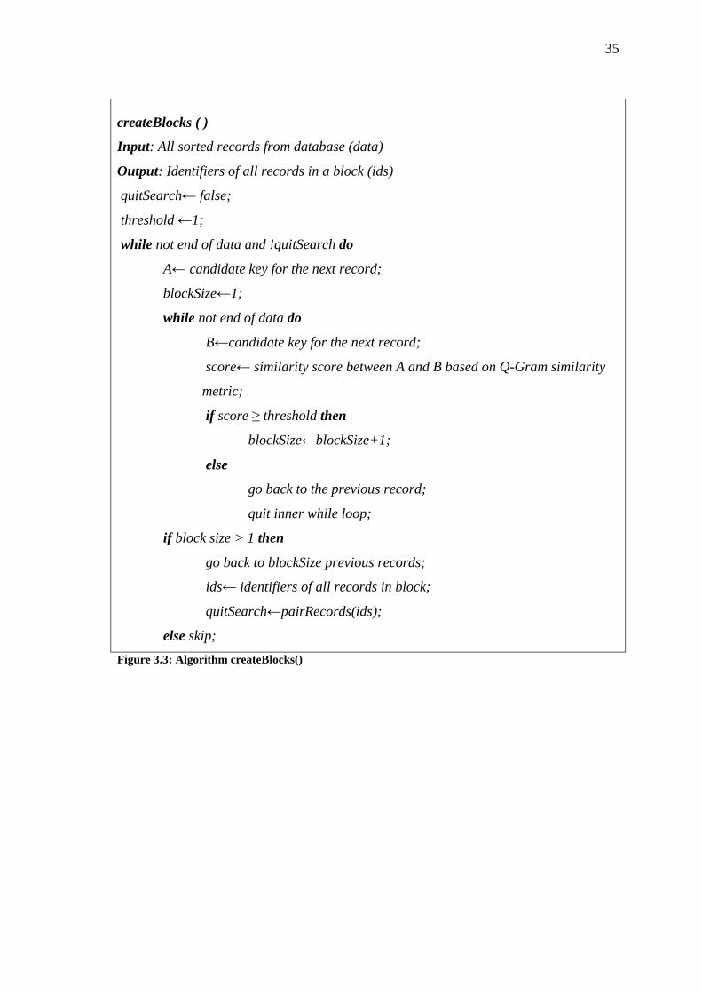
Standard blocking technique: blocking technique doesn't include all the records from

the database in the created blocks, which means that there are records that don’t belong

to any blocks. In this case these records are ignored. Also, all the blocks are non-

overlapping windows. As shown in Figure 3.3.

To create the blocks, first we retrieve the first record and the second record from the

database. Then, we compare the candidate key of first record with the candidate key of

the second record and compute the similarity score between the two keys using the Q-

Gram metric. If the similarity score is equal to one, the two records are put into the

same block. After that we repeat the comparison with the third record and so on. If no

records satisfy the similarity with candidate key of the first record, we used the next

record to create a new block. Once a new block is found, we retrieve the identifiers of

all records in the block and sent them to be paired.

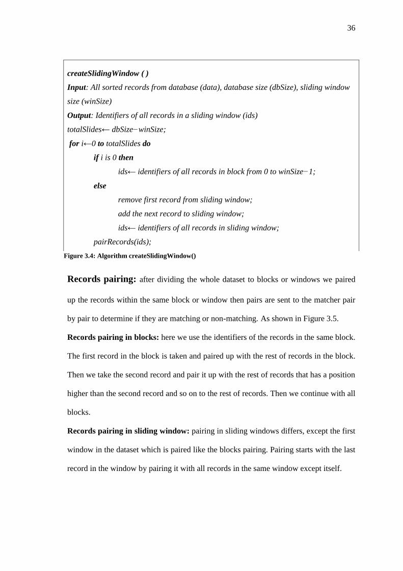
Sorted-Neighborhood technique: unlike the standard blocking technique, the sliding

window has a fixed size, each time the window slides down first record is removed

from the window, and the next record is added to the window, and to the list of

identifiers. These identifiers passed to the record pairing stage. As shown in Figure 3.4.

35

createBlocks ( )

Input: All sorted records from database (data)

Output: Identifiers of all records in a block (ids)

quitSearch← false;

threshold ←1;

while not end of data and !quitSearch do

A← candidate key for the next record;

blockSize←1;

while not end of data do

B←candidate key for the next record;

score← similarity score between A and B based on Q-Gram similarity

metric;

if score ≥ threshold then

blockSize←blockSize+1;

else

go back to the previous record;

quit inner while loop;

if block size > 1 then

go back to blockSize previous records;

ids← identifiers of all records in block;

quitSearch←pairRecords(ids);

else skip;

Figure 3.3: Algorithm createBlocks()

36

Records pairing: after dividing the whole dataset to blocks or windows we paired

up the records within the same block or window then pairs are sent to the matcher pair

by pair to determine if they are matching or non-matching. As shown in Figure 3.5.

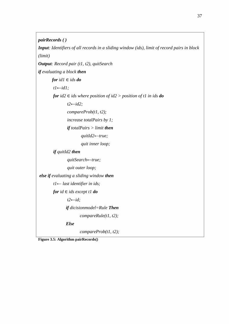
Records pairing in blocks: here we use the identifiers of the records in the same block.

The first record in the block is taken and paired up with the rest of records in the block.

Then we take the second record and pair it up with the rest of records that has a position

higher than the second record and so on to the rest of records. Then we continue with all

blocks.

Records pairing in sliding window: pairing in sliding windows differs, except the first

window in the dataset which is paired like the blocks pairing. Pairing starts with the last

record in the window by pairing it with all records in the same window except itself.

createSlidingWindow ( )

Input: All sorted records from database (data), database size (dbSize), sliding window

size (winSize)

Output: Identifiers of all records in a sliding window (ids)

totalSlides← dbSize−winSize;

for i←0 to totalSlides do

if i is 0 then

ids← identifiers of all records in block from 0 to winSize−1;

else

remove first record from sliding window;

add the next record to sliding window;

ids← identifiers of all records in sliding window;

pairRecords(ids);

Figure 3.4: Algorithm createSlidingWindow()

37

pairRecords ( )

Input: Identifiers of all records in a sliding window (ids), limit of record pairs in block

(limit)

Output: Record pair (t1, t2), quitSearch

if evaluating a block then

for id1 ids do

t1←id1;

for id2 ids where position of id2 > position of t1 in ids do

t2←id2;

compareProb(t1, t2);

increase totalPairs by 1;

if totalPairs > limit then

quitId2←true;

quit inner loop;

if quitId2 then

quitSearch←true;

quit outer loop;

else if evaluating a sliding window then

t1← last identifier in ids;

for id ids except t1 do

t2←id;

if dicisionmodel=Rule Then

compareRule(t1, t2);

Else

compareProb(t1, t2);

Figure 3.5: Algorithm pairRecords()

38

Threshold generator for Probabilistic-based technique: the Probabilistic-

based technique needs to compute the threshold value, this done using the EM

algorithm which use the standard blocking to pair up the records. The threshold value

computes by these steps:

1. Compute the vector pattern of each record pairs that we get from the blocks by

comparing the similarity score of each attribute of the record pair with a

threshold value. If the score of the attribute above the threshold the value of this

attribute is set to 1. Otherwise, it's set to 0. So we get from the record pair a

vector pattern consists of binary values. Then we store all the vector patterns and

their frequency counts.

2. Estimate the value of mi and the value of ui from the vector patterns and their

frequency counts. As shown in Figure 3.6.

3. Compute the threshold value using the values of mi and ui. As shown in Figure

3.9.

The values of mi and ui could be estimated by converting the record pairs from the

blocks to vector patterns. We store the vector patterns as a binary model and the

frequency counts. If record pair generates a comparison vector in the binary model a

count of one is added to the frequency count of that particular pattern. Otherwise, we

add the pattern and a frequency count of one.

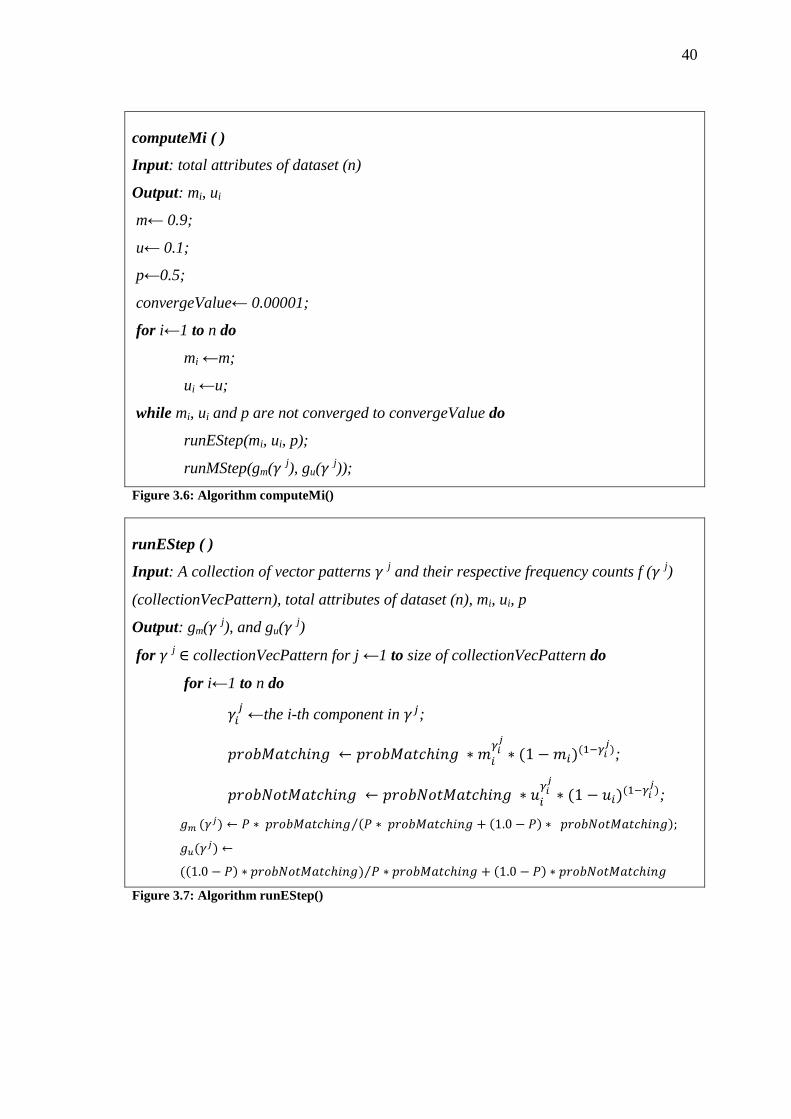
EM algorithm makes use of patterns and their frequency counts, by applying these

equations to estimate mi and ui after initialize mi, ui, and p were 0.9, 0.1, and 0.5

respectively using the E-step and M-step (Jaro, 1989). As shown in Figures 3.7, and 3.8.

(3.1)

(3.2)

39

(3.3)

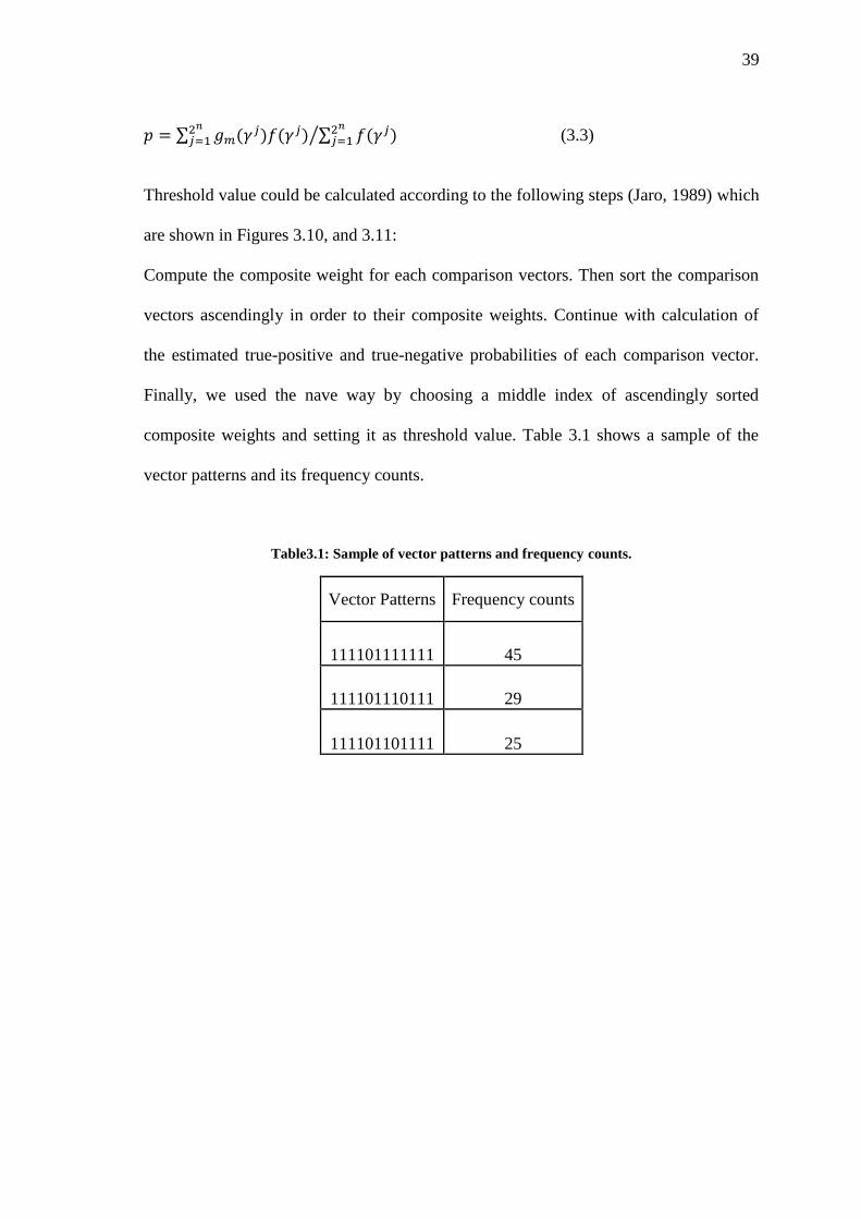
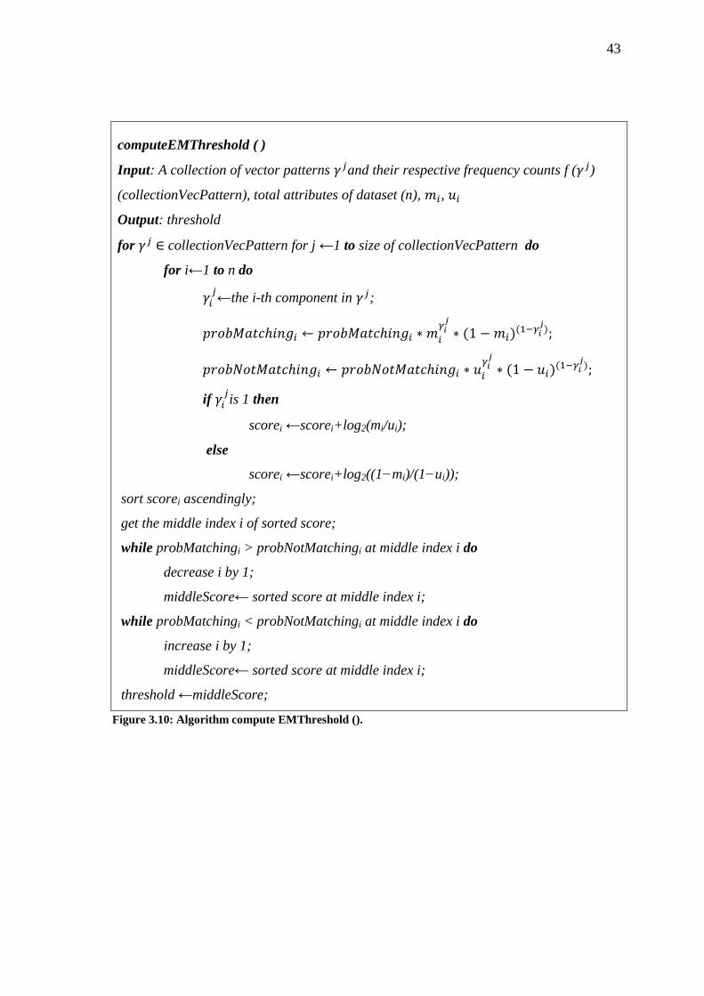
Threshold value could be calculated according to the following steps (Jaro, 1989) which

are shown in Figures 3.10, and 3.11:

Compute the composite weight for each comparison vectors. Then sort the comparison

vectors ascendingly in order to their composite weights. Continue with calculation of

the estimated true-positive and true-negative probabilities of each comparison vector.

Finally, we used the nave way by choosing a middle index of ascendingly sorted

composite weights and setting it as threshold value. Table 3.1 shows a sample of the

vector patterns and its frequency counts.

Table3.1: Sample of vector patterns and frequency counts.

Vector Patterns Frequency counts

111101111111 45

111101110111 29

111101101111 25

40

computeMi ( )

Input: total attributes of dataset (n)

Output: mi, ui

m← 0.9;

u← 0.1;

p←0.5;

convergeValue← 0.00001;

for i←1 to n do

mi ←m;

ui ←u;

while mi, ui and p are not converged to convergeValue do

runEStep(mi, ui, p);

runMStep(gm( j), gu(

j));

Figure 3.6: Algorithm computeMi()

runEStep ( )

Input: A collection of vector patterns j and their respective frequency counts f (

j)

(collectionVecPattern), total attributes of dataset (n), mi, ui, p

Output: gm( j), and gu(

j)

for j collectionVecPattern for j ←1 to size of collectionVecPattern do

for i←1 to n do

←the i-th component in ;

;

;

Figure 3.7: Algorithm runEStep()

41

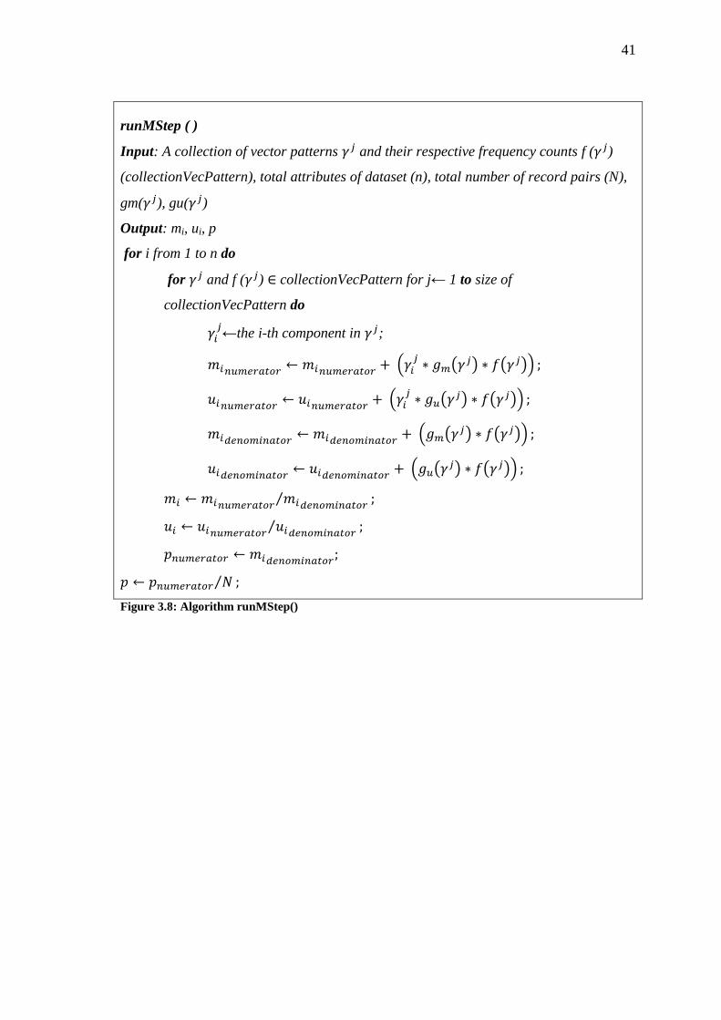
runMStep ( )

Input: A collection of vector patterns and their respective frequency counts f ( )

(collectionVecPattern), total attributes of dataset (n), total number of record pairs (N),

gm( ), gu( )

Output: mi, ui, p

for i from 1 to n do

for and f ( ) collectionVecPattern for j← 1 to size of

collectionVecPattern do

←the i-th component in ;

Figure 3.8: Algorithm runMStep()

42

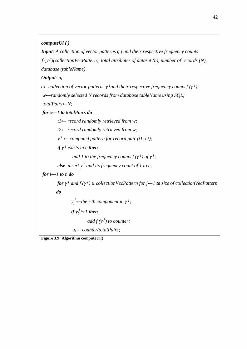
computeUi ( )

Input: A collection of vector patterns g j and their respective frequency counts

(collectionVecPattern), total attributes of dataset (n), number of records (N),

database (tableName)

Output: ui

c←collection of vector patterns and their respective frequency counts f ( );

w←randomly selected N records from database tableName using SQL;

totalPairs←N;

for x←1 to totalPairs do

t1← record randomly retrieved from w;

t2← record randomly retrieved from w;

← computed pattern for record pair (t1, t2);

if exists in c then

add 1 to the frequency counts f ( ) of ;

else insert and its frequency count of 1 to c;

for i←1 to n do

for and f ( ) collectionVecPattern for j←1 to size of collectionVecPattern

do

←the i-th component in ;

if is 1 then

add f ( ) to counter;

ui ←counter/totalPairs;

Figure 3.9: Algorithm computeUi()

43

computeEMThreshold ( )

Input: A collection of vector patterns and their respective frequency counts f ( )

(collectionVecPattern), total attributes of dataset (n), ,

Output: threshold

for collectionVecPattern for j ←1 to size of collectionVecPattern do

for i←1 to n do

←the i-th component in ;

if is 1 then

scorei ←scorei+log2(mi/ui);

else

scorei ←scorei+log2((1−mi)/(1−ui));

sort scorei ascendingly;

get the middle index i of sorted score;

while probMatchingi > probNotMatchingi at middle index i do

decrease i by 1;

middleScore← sorted score at middle index i;

while probMatchingi < probNotMatchingi at middle index i do

increase i by 1;

middleScore← sorted score at middle index i;

threshold ←middleScore;

Figure 3.10: Algorithm compute EMThreshold ().

44

Decision models matcher: in this stage the user selects the decision model that

decides if the record pair conceder to be matched or non-matched.

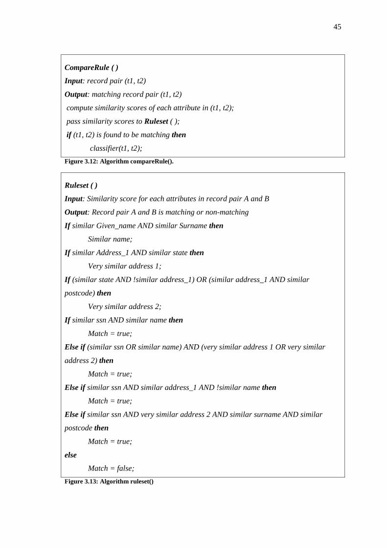
Rule-Based matcher: the Rule-based matcher works as following: (as shown in Figure

3.12)

1. Create the Equational Theory rules. According to our datasets the rules focus on

names similarity (Given name, Surname), addresses similarity (Street number,

Address 1, Suburb, Postcode, State), and social security number similarity.

2. Set the threshold value.

3. Receiving the pairs of records paired up from the SN technique.

4. Calculate the similarity score for each attribute of each record pair.

5. Compare the attribute score which is used in the rules with the (ET) rules and

the threshold value. As shown in Figure 3.13.

6. If the pair is matched then pass it to the classification stage.

For multi-pass SN technique repeat steps 3 to 6.

computeCompositeWeight ( )

Input: total attributes of dataset (n), vector pattern of a record pair (pattern), mi, ui,

record pair (t1, t2)

Output: composite score of record pair (score)

for i←1 to n do

patterni ← the i-th component in pattern;

if patterni is 1 then

scorei ←scorei+log2(mi/ui);

else

scorei ←scorei+log2((1−mi)/(1−ui));

return score;

Figure 3.11: Algorithm computeCompositeWeight ().

45

CompareRule ( )

Input: record pair (t1, t2)

Output: matching record pair (t1, t2)

compute similarity scores of each attribute in (t1, t2);

pass similarity scores to Ruleset ( );

if (t1, t2) is found to be matching then

classifier(t1, t2);

Figure 3.12: Algorithm compareRule().

Ruleset ( )

Input: Similarity score for each attributes in record pair A and B

Output: Record pair A and B is matching or non-matching

If similar Given_name AND similar Surname then

Similar name;

If similar Address_1 AND similar state then

Very similar address 1;

If (similar state AND !similar address_1) OR (similar address_1 AND similar

postcode) then

Very similar address 2;

If similar ssn AND similar name then

Match = true;

Else if (similar ssn OR similar name) AND (very similar address 1 OR very similar

address 2) then

Match = true;

Else if similar ssn AND similar address_1 AND !similar name then

Match = true;

Else if similar ssn AND very similar address 2 AND similar surname AND similar

postcode then

Match = true;

else

Match = false;

Figure 3.13: Algorithm ruleset()

46

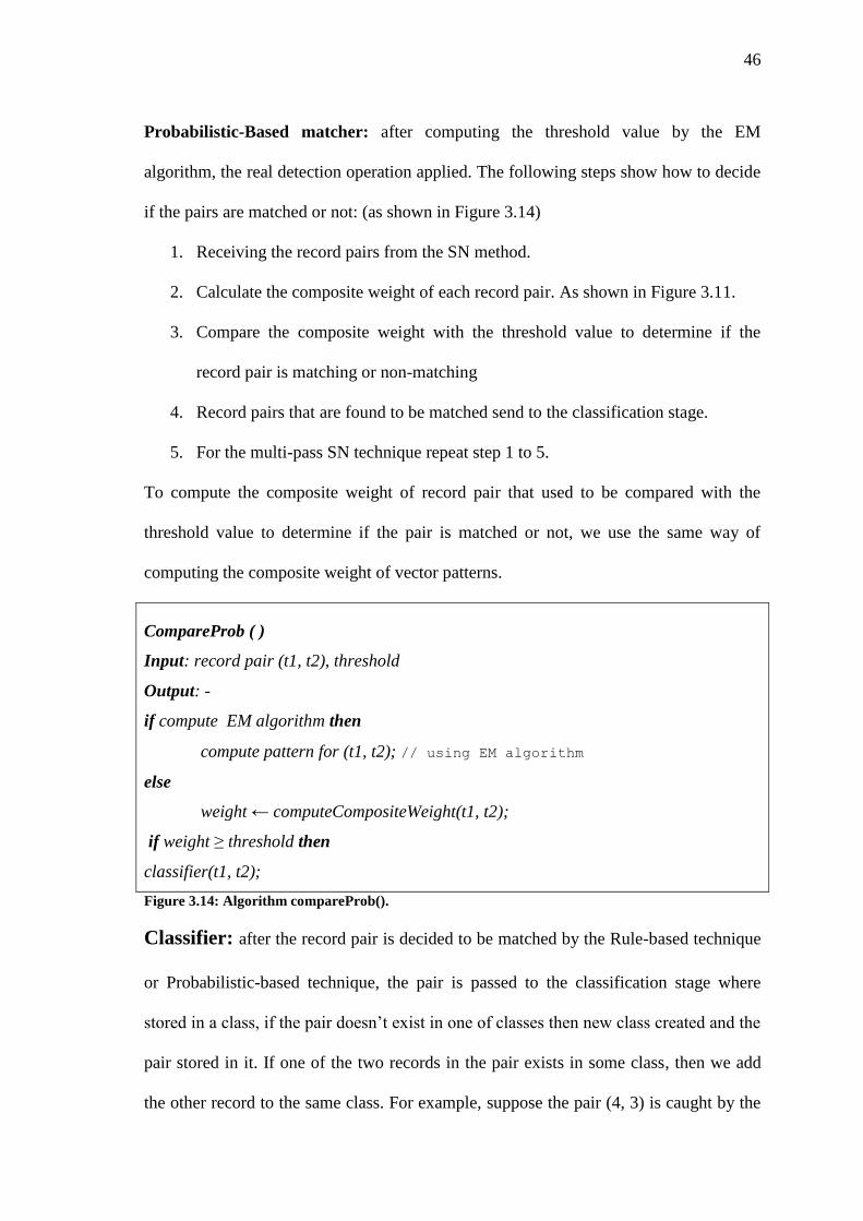
Probabilistic-Based matcher: after computing the threshold value by the EM

algorithm, the real detection operation applied. The following steps show how to decide

if the pairs are matched or not: (as shown in Figure 3.14)

1. Receiving the record pairs from the SN method.

2. Calculate the composite weight of each record pair. As shown in Figure 3.11.

3. Compare the composite weight with the threshold value to determine if the

record pair is matching or non-matching

4. Record pairs that are found to be matched send to the classification stage.

5. For the multi-pass SN technique repeat step 1 to 5.

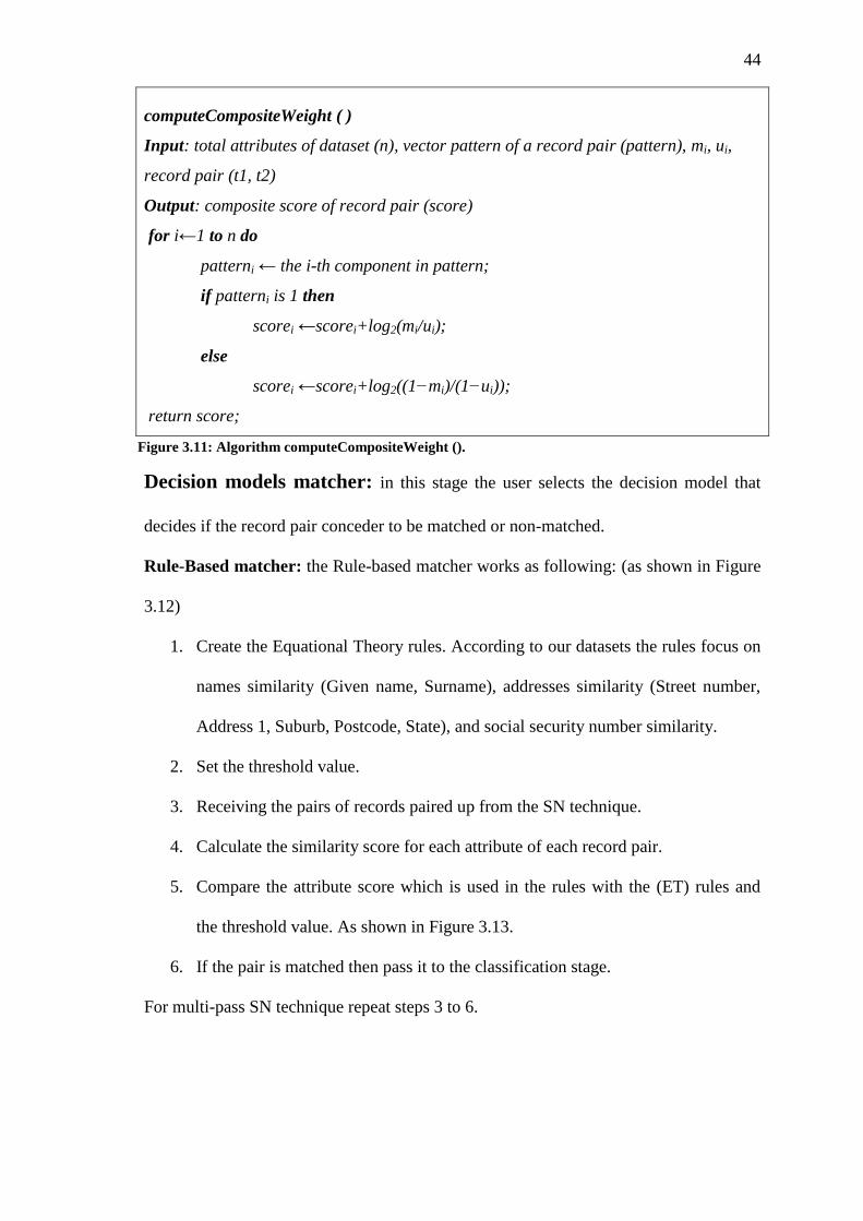
To compute the composite weight of record pair that used to be compared with the

threshold value to determine if the pair is matched or not, we use the same way of

computing the composite weight of vector patterns.

CompareProb ( )

Input: record pair (t1, t2), threshold

Output: -

if compute EM algorithm then

compute pattern for (t1, t2); // using EM algorithm

else

weight ← computeCompositeWeight(t1, t2);

if weight ≥ threshold then

classifier(t1, t2);

Figure 3.14: Algorithm compareProb().

Classifier: after the record pair is decided to be matched by the Rule-based technique

or Probabilistic-based technique, the pair is passed to the classification stage where

stored in a class, if the pair doesn’t exist in one of classes then new class created and the

pair stored in it. If one of the two records in the pair exists in some class, then we add

the other record to the same class. For example, suppose the pair (4, 3) is caught by the

47

Matcher. Next, the pair (5, 2) is caught. At this point, the two pairs are stored in two

different classes. In the next matching process, the pair (5, 4) is caught. Since record 4

points to class A whilst record 5 points to the class B, we join both Sets together. What

we get in the end is Set A consisting of records {2, 3, 4, 5}. As shown in Figure 3.15.

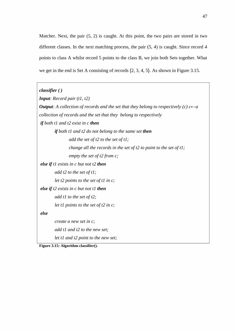
classifier ( )

Input: Record pair (t1, t2)

Output: A collection of records and the set that they belong to respectively (c) c←a

collection of records and the set that they belong to respectively

if both t1 and t2 exist in c then

if both t1 and t2 do not belong to the same set then

add the set of t2 to the set of t1;

change all the records in the set of t2 to point to the set of t1;

empty the set of t2 from c;

else if t1 exists in c but not t2 then

add t2 to the set of t1;

let t2 points to the set of t1 in c;

else if t2 exists in c but not t1 then

add t1 to the set of t2;

let t1 points to the set of t2 in c;

else

create a new set in c;

add t1 and t2 to the new set;

let t1 and t2 point to the new set;

Figure 3.15: Algorithm classifier().

48

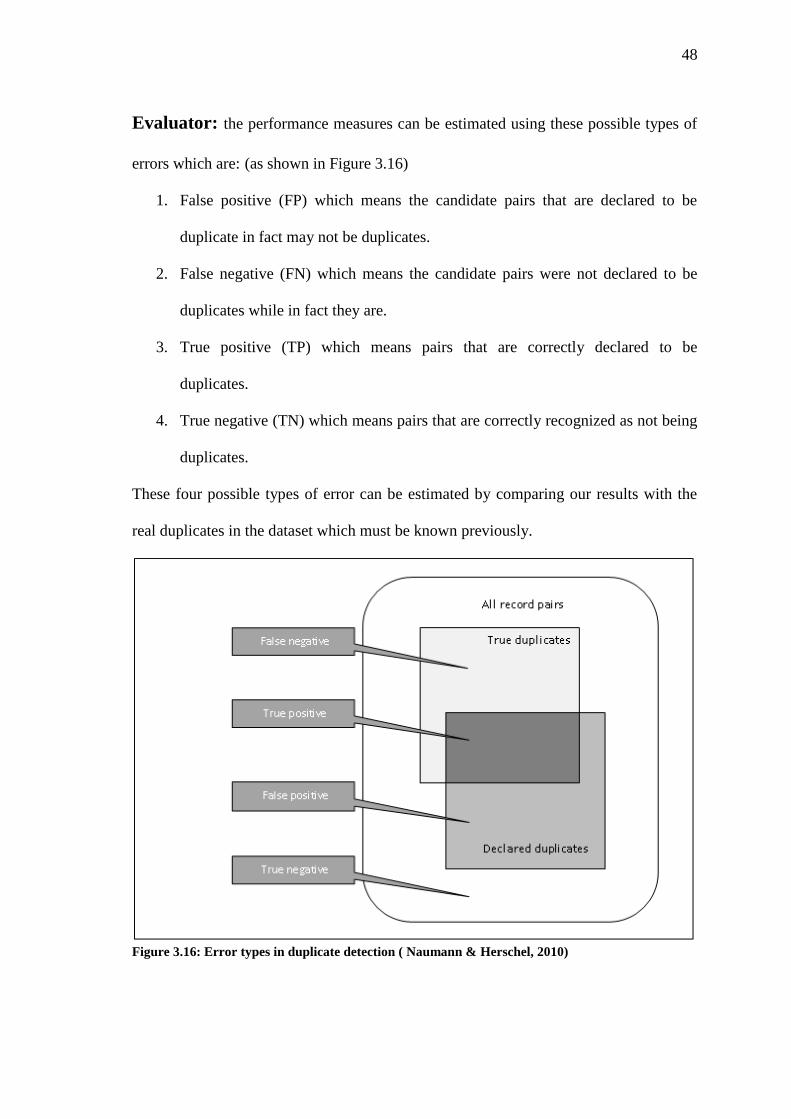
Evaluator: the performance measures can be estimated using these possible types of

errors which are: (as shown in Figure 3.16)

1. False positive (FP) which means the candidate pairs that are declared to be

duplicate in fact may not be duplicates.

2. False negative (FN) which means the candidate pairs were not declared to be

duplicates while in fact they are.

3. True positive (TP) which means pairs that are correctly declared to be

duplicates.

4. True negative (TN) which means pairs that are correctly recognized as not being

duplicates.

These four possible types of error can be estimated by comparing our results with the

real duplicates in the dataset which must be known previously.

Figure 3.16: Error types in duplicate detection ( Naumann & Herschel, 2010)

49

Chapter 4

Experimental Evaluation

In this chapter, we present the conducted experiments with their used settings and their

results. We have used a synthetic dataset that was previously used as a benchmark in

some of related work. In Section 4.1, dataset is presented in detail. In Section 4.2, the

development environment is presented. The experiments in Section 4.3 evaluate the

performance of the two duplication detection techniques, the Rule-based, and

Probabilistic-based, on two different datasets using standard measures of accuracy,

efficiency, and quality.

4.1 Data Set

There are a few datasets used by previous researchers are available to download on the

Internet. One of these limited datasets is FEBRL (Freely Extensible Biomedical Record

Linkage). This dataset is a synthetic one it contains patients' data such as given name,

surname, street number, addresse1, address2, suburb, postcode, state name, date of

birth, age, phone number, and social security number.

In this study two datasets of FEBRL have been used; the first (DATASET_A) contains

10000 records with 5000 original records and 5000 duplicated records. There is one

duplicate per original record, maximum one modification per duplicate record and

maximum one modification per attribute. The second (DATASET_B) contains 10000

records with 6000 original records and 4000 duplicated records. There is up to nine

duplicates for an original record, maximum three modifications per attribute, and

maximum 10 modifications per record. Table 4.1 shows a sample of duplicate records

from this dataset.

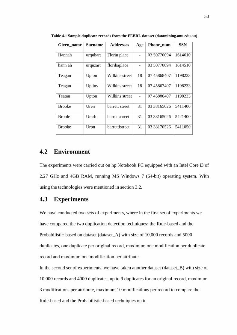
50

Table 4.1 Sample duplicate records from the FEBRL dataset (datamining.anu.edu.au)

Given_name Surname Addresses Age Phone_num SSN

Hannah urquhart Florin place - 03 50770094 1614610

hann ah urquzart florihaplace - 03 50770094 1614510

Teagan Upton Wilkins street 18 07 45868407 1198233

Teagan Uptiny Wilkins street 18 07 45867407 1198233

Teatan Upton Wilkins street - 07 45886407 1198233

Brooke Uren barrett street 31 03 38165026 5411400

Broole Umrh barrettaareet 31 03 38165026 5421400

Brooke Urpn barrettistreet 31 03 38170526 5411050

4.2 Environment

The experiments were carried out on hp Notebook PC equipped with an Intel Core i3 of

2.27 GHz and 4GB RAM, running MS Windows 7 (64-bit) operating system. With

using the technologies were mentioned in section 3.2.

4.3 Experiments

We have conducted two sets of experiments, where in the first set of experiments we

have compared the two duplication detection techniques: the Rule-based and the

Probabilistic-based on dataset (dataset_A) with size of 10,000 records and 5000

duplicates, one duplicate per original record, maximum one modification per duplicate

record and maximum one modification per attribute.

In the second set of experiments, we have taken another dataset (dataset_B) with size of

10,000 records and 4000 duplicates, up to 9 duplicates for an original record, maximum

3 modifications per attribute, maximum 10 modifications per record to compare the

Rule-based and the Probabilistic-based techniques on it.

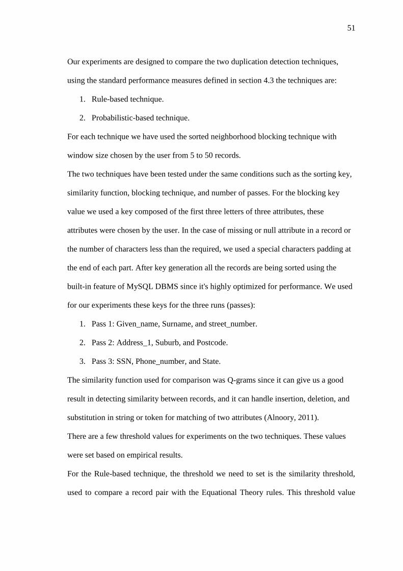
51

Our experiments are designed to compare the two duplication detection techniques,

using the standard performance measures defined in section 4.3 the techniques are:

1. Rule-based technique.

2. Probabilistic-based technique.

For each technique we have used the sorted neighborhood blocking technique with

window size chosen by the user from 5 to 50 records.

The two techniques have been tested under the same conditions such as the sorting key,

similarity function, blocking technique, and number of passes. For the blocking key

value we used a key composed of the first three letters of three attributes, these

attributes were chosen by the user. In the case of missing or null attribute in a record or

the number of characters less than the required, we used a special characters padding at

the end of each part. After key generation all the records are being sorted using the

built-in feature of MySQL DBMS since it's highly optimized for performance. We used

for our experiments these keys for the three runs (passes):

1. Pass 1: Given_name, Surname, and street_number.

2. Pass 2: Address_1, Suburb, and Postcode.

3. Pass 3: SSN, Phone_number, and State.

The similarity function used for comparison was Q-grams since it can give us a good

result in detecting similarity between records, and it can handle insertion, deletion, and

substitution in string or token for matching of two attributes (Alnoory, 2011).

There are a few threshold values for experiments on the two techniques. These values

were set based on empirical results.

For the Rule-based technique, the threshold we need to set is the similarity threshold,

used to compare a record pair with the Equational Theory rules. This threshold value

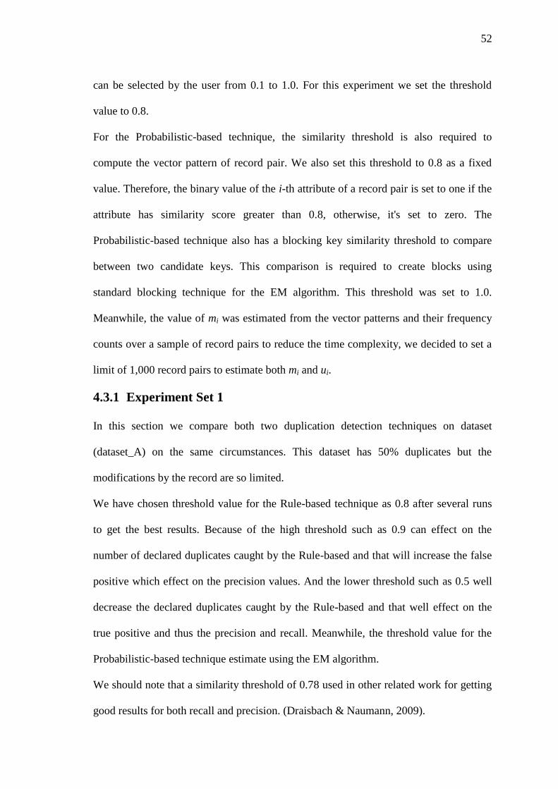
52

can be selected by the user from 0.1 to 1.0. For this experiment we set the threshold

value to 0.8.

For the Probabilistic-based technique, the similarity threshold is also required to

compute the vector pattern of record pair. We also set this threshold to 0.8 as a fixed

value. Therefore, the binary value of the i-th attribute of a record pair is set to one if the

attribute has similarity score greater than 0.8, otherwise, it's set to zero. The

Probabilistic-based technique also has a blocking key similarity threshold to compare

between two candidate keys. This comparison is required to create blocks using

standard blocking technique for the EM algorithm. This threshold was set to 1.0.

Meanwhile, the value of mi was estimated from the vector patterns and their frequency

counts over a sample of record pairs to reduce the time complexity, we decided to set a

limit of 1,000 record pairs to estimate both mi and ui.

4.3.1 Experiment Set 1

In this section we compare both two duplication detection techniques on dataset

(dataset_A) on the same circumstances. This dataset has 50% duplicates but the

modifications by the record are so limited.

We have chosen threshold value for the Rule-based technique as 0.8 after several runs

to get the best results. Because of the high threshold such as 0.9 can effect on the

number of declared duplicates caught by the Rule-based and that will increase the false

positive which effect on the precision values. And the lower threshold such as 0.5 well

decrease the declared duplicates caught by the Rule-based and that well effect on the

true positive and thus the precision and recall. Meanwhile, the threshold value for the

Probabilistic-based technique estimate using the EM algorithm.

We should note that a similarity threshold of 0.78 used in other related work for getting

good results for both recall and precision. (Draisbach & Naumann, 2009).

53

Experiment 1-A

Duplication detection techniques used blocking techniques to avoid comparing all

records with each other to increase the efficiency of the duplication detection technique.

As shown in table 4.2.

In Figure 4.1, we clarify the effect of varying the window size from 5 records per the

window to 50 records per the window on both recall, and precision. Increasing the

window size will increase the pairs numbers that will compared together to find the

duplicates records. And that will give us surely better results depending on the dataset

size and the percentage of duplicates records in this dataset. But it will affect the

runtime of the duplicate detection.

Table 4.2: Total number of detected duplicates with varying window size for Dataset_A.

Window size 5 10 15 20 25 30 35 40 45 50

Rule true duplicates 3541 3562 3566 3570 3577 3585 3594 3607 3624 3628

Prob true duplicates 3834 4019 4169 4224 4302 4316 4342 4360 4381 4394

54

Figure 4.1:Accuracy comparison between Rule-based and Probabilistic-based with varying window

size for dataset_A.

Experiment 1-B

To measure the effect of dataset size on the two techniques we conduct another

experiment by increasing the number of records from 1000 records to 10,000 records.

Figure 4.2 clarifies the accuracy for both duplication detection techniques according to

dataset size. Probabilistic-based techniques use the frequency of matched (mi) and

unmatched (ui) for each attribute to estimate the weight of every attribute in the record

and make use of these values to compute the threshold value. Therefore, the size of

dataset well effect distributing of errors within the attributes. Meanwhile, the Rule-

based depends on the quality of the pairs to compare with the rules, so it's slightly

affected by changing the size of dataset.

75%

80%

85%

90%

95%

100%

5 10 15 20 25 30 35 40 45 50 55

Acc

ura

cy

window size

Rule-Recall

Prob-Recall

Rule-Precision

Prob-Precision

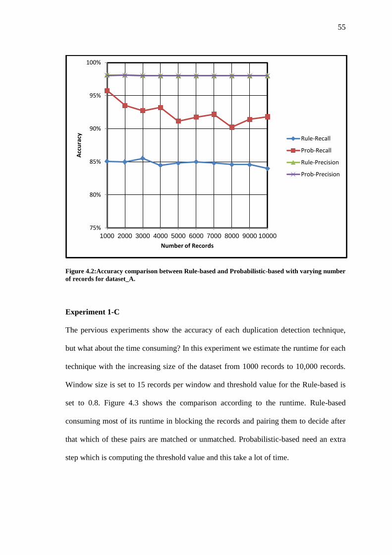
55

Figure 4.2:Accuracy comparison between Rule-based and Probabilistic-based with varying number

of records for dataset_A.

Experiment 1-C

The pervious experiments show the accuracy of each duplication detection technique,

but what about the time consuming? In this experiment we estimate the runtime for each

technique with the increasing size of the dataset from 1000 records to 10,000 records.

Window size is set to 15 records per window and threshold value for the Rule-based is

set to 0.8. Figure 4.3 shows the comparison according to the runtime. Rule-based

consuming most of its runtime in blocking the records and pairing them to decide after

that which of these pairs are matched or unmatched. Probabilistic-based need an extra

step which is computing the threshold value and this take a lot of time.

75%

80%

85%

90%

95%

100%

1000 2000 3000 4000 5000 6000 7000 8000 9000 10000

Acc

ura

cy

Number of Records

Rule-Recall

Prob-Recall

Rule-Precision

Prob-Precision

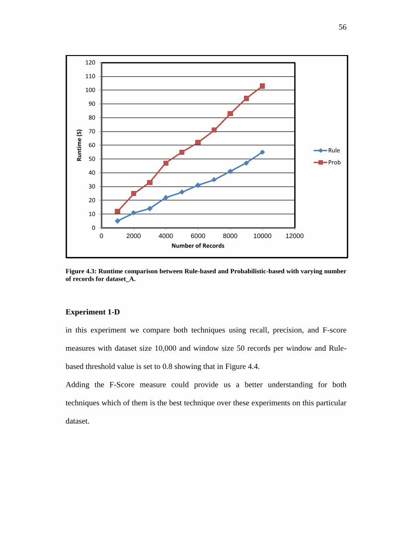
56

Figure 4.3: Runtime comparison between Rule-based and Probabilistic-based with varying number

of records for dataset_A.

Experiment 1-D

in this experiment we compare both techniques using recall, precision, and F-score

measures with dataset size 10,000 and window size 50 records per window and Rule-

based threshold value is set to 0.8 showing that in Figure 4.4.

Adding the F-Score measure could provide us a better understanding for both

techniques which of them is the best technique over these experiments on this particular

dataset.

0

10

20

30

40

50

60

70

80

90

100

110

120

0 2000 4000 6000 8000 10000 12000

Ru

nti

me

(S)

Number of Records

Rule

Prob

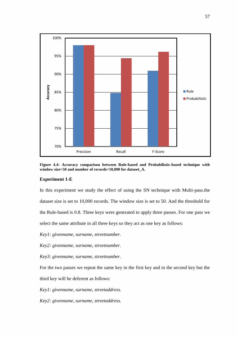
57

Figure 4.4: Accuracy comparison between Rule-based and Probabilistic-based technique with

window size=50 and number of records=10,000 for dataset_A.

Experiment 1-E

In this experiment we study the effect of using the SN technique with Multi-pass.the

dataset size is set to 10,000 records. The window size is set to 50. And the threshold for

the Rule-based is 0.8. Three keys were generated to apply three passes. For one pass we

select the same attribute in all three keys so they act as one key as follows:

Key1: givenname, surname, streetnumber.

Key2: givenname, surname, streetnumber.

Key3: givenname, surname, streetnumber.

For the two passes we repeat the same key in the first key and in the second key but the

third key will be deferent as follows:

Key1: givenname, surname, streetaddress.

Key2: givenname, surname, streetaddress.

70%

75%

80%

85%

90%

95%

100%

Precision Recall F-Score

Acc

ura

cy

Rule

Probabilistic

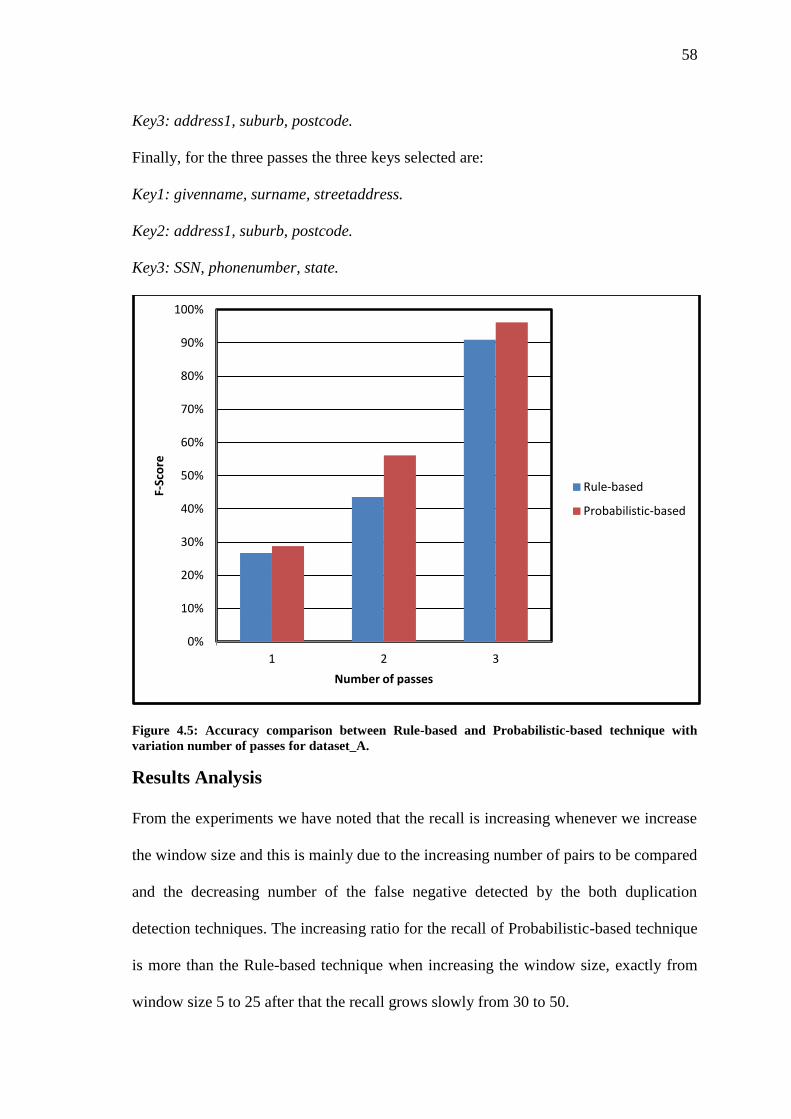
58

Key3: address1, suburb, postcode.

Finally, for the three passes the three keys selected are:

Key1: givenname, surname, streetaddress.

Key2: address1, suburb, postcode.

Key3: SSN, phonenumber, state.

Figure 4.5: Accuracy comparison between Rule-based and Probabilistic-based technique with

variation number of passes for dataset_A.

Results Analysis

From the experiments we have noted that the recall is increasing whenever we increase

the window size and this is mainly due to the increasing number of pairs to be compared

and the decreasing number of the false negative detected by the both duplication

detection techniques. The increasing ratio for the recall of Probabilistic-based technique

is more than the Rule-based technique when increasing the window size, exactly from

window size 5 to 25 after that the recall grows slowly from 30 to 50.

0%

10%

20%

30%

40%

50%

60%

70%

80%

90%

100%

1 2 3

F-Sc

ore

Number of passes

Rule-based

Probabilistic-based

59

Comparing the results for the precision, we have noted that precision stays stable when

increasing the window size with insignificant change because of the stability of

the number of false positive.

The increasing of dataset size shows that the overall values of recall slightly decreased

for both techniques, but the decreasing of Probabilistic-based technique is not a linear

and that refers to the number of pairs (sample of all pairs) that used to estimate the

threshold value by the EM algorithm using standard blocking technique. Number of

pairs that used to compute the threshold value for dataset size 1000 records is 427 pair

from 427 total pairs so this sample will give us result better than dataset with size

10,000 records which has 4123 pairs with sample 1000 pairs. Therefore, the recall

decreased when increasing dataset size but in irregular shape. Table 4.3 views the pairs

for the dataset with varying size.

Table 4.3: Sample of pairs for the EM algorithm for dataset_A.

Number of records Number of pairs Sample of pairs

1000 427 427

2500 1067 1000

5000 2088 1000

10,000 4123 1000

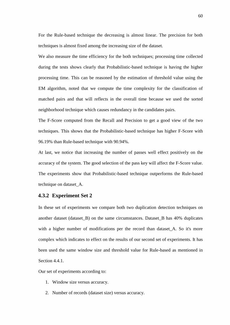
60

For the Rule-based technique the decreasing is almost linear. The precision for both

techniques is almost fixed among the increasing size of the dataset.

We also measure the time efficiency for the both techniques; processing time collected

during the tests shows clearly that Probabilistic-based technique is having the higher

processing time. This can be reasoned by the estimation of threshold value using the

EM algorithm, noted that we compute the time complexity for the classification of

matched pairs and that will reflects in the overall time because we used the sorted

neighborhood technique which causes redundancy in the candidates pairs.

The F-Score computed from the Recall and Precision to get a good view of the two

techniques. This shows that the Probabilistic-based technique has higher F-Score with

96.19% than Rule-based technique with 90.94%.

At last, we notice that increasing the number of passes well effect positively on the

accuracy of the system. The good selection of the pass key will affect the F-Score value.

The experiments show that Probabilistic-based technique outperforms the Rule-based

technique on dataset_A.

4.3.2 Experiment Set 2

In these set of experiments we compare both two duplication detection techniques on

another dataset (dataset_B) on the same circumstances. Dataset_B has 40% duplicates

with a higher number of modifications per the record than dataset_A. So it's more

complex which indicates to effect on the results of our second set of experiments. It has

been used the same window size and threshold value for Rule-based as mentioned in

Section 4.4.1.

Our set of experiments according to:

1. Window size versus accuracy.

2. Number of records (dataset size) versus accuracy.

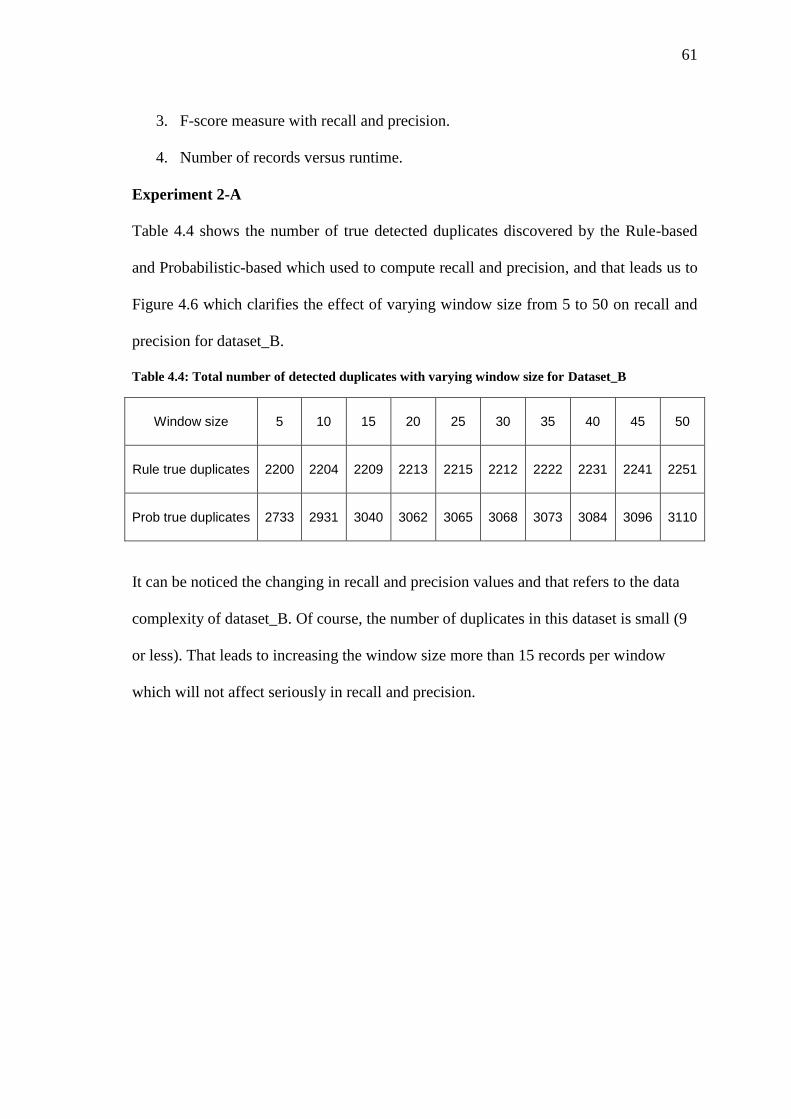
61

3. F-score measure with recall and precision.

4. Number of records versus runtime.

Experiment 2-A

Table 4.4 shows the number of true detected duplicates discovered by the Rule-based

and Probabilistic-based which used to compute recall and precision, and that leads us to

Figure 4.6 which clarifies the effect of varying window size from 5 to 50 on recall and

precision for dataset_B.

Table 4.4: Total number of detected duplicates with varying window size for Dataset_B

Window size 5 10 15 20 25 30 35 40 45 50

Rule true duplicates 2200 2204 2209 2213 2215 2212 2222 2231 2241 2251

Prob true duplicates 2733 2931 3040 3062 3065 3068 3073 3084 3096 3110

It can be noticed the changing in recall and precision values and that refers to the data

complexity of dataset_B. Of course, the number of duplicates in this dataset is small (9

or less). That leads to increasing the window size more than 15 records per window

which will not affect seriously in recall and precision.

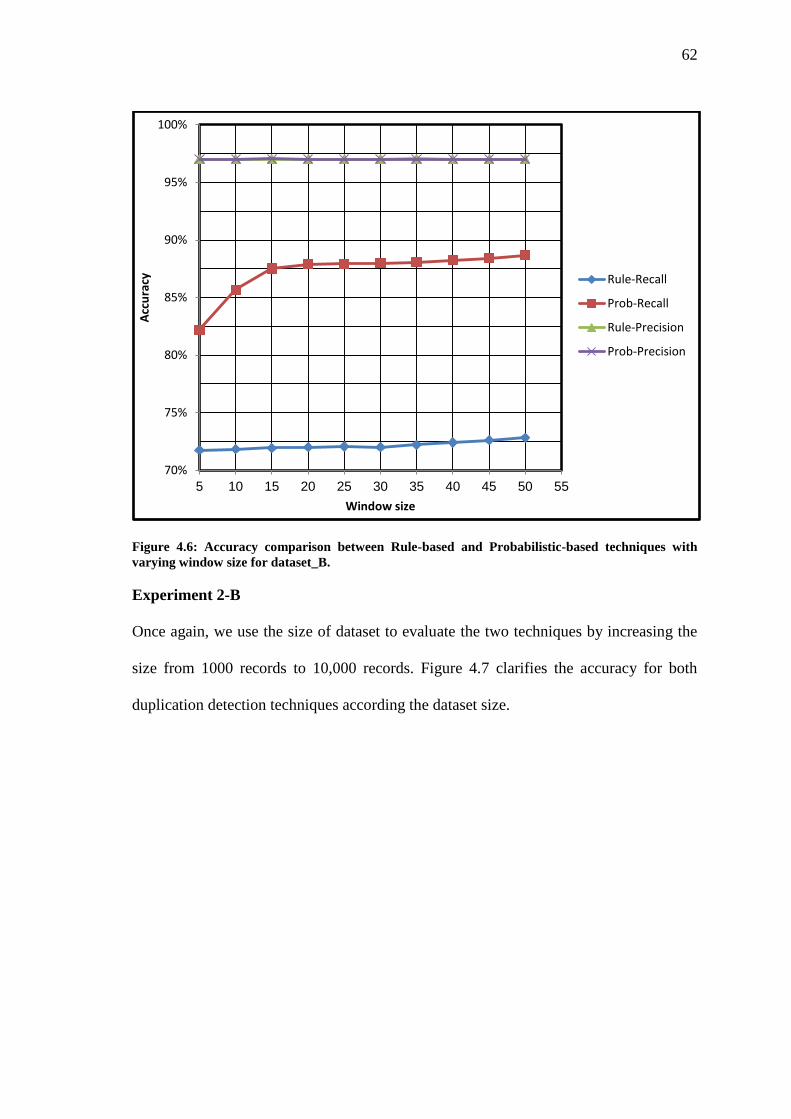
62

Figure 4.6: Accuracy comparison between Rule-based and Probabilistic-based techniques with

varying window size for dataset_B.

Experiment 2-B

Once again, we use the size of dataset to evaluate the two techniques by increasing the

size from 1000 records to 10,000 records. Figure 4.7 clarifies the accuracy for both

duplication detection techniques according the dataset size.

70%

75%

80%

85%

90%

95%

100%

5 10 15 20 25 30 35 40 45 50 55

Acc

ura

cy

Window size

Rule-Recall

Prob-Recall

Rule-Precision

Prob-Precision

63

Figure 4.7: Accuracy comparison between Rule-based and Probabilistic-based techniques with

varying number of records for dataset_B.

Experiment 2-C

And finally, the pervious experiments show the accuracy of each duplication detection

technique, but what about the time consuming?

In this experiment, we estimate the runtime for each technique with the increasing size

of the dataset from 1000 records to 10,000 records. Figure 4.8 shows the comparison

according to the runtime.

60%

65%

70%

75%

80%

85%

90%

95%

100%

1000 2000 3000 4000 5000 6000 7000 8000 9000 10000

Acc

ura

cy

Number o Records

Rule-Recall

Prob-Recall

Rule-Precision

Prob-Precision

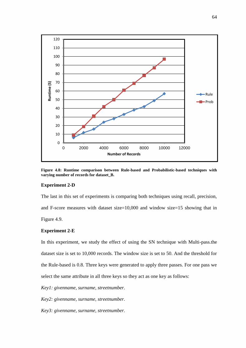
64

Figure 4.8: Runtime comparison between Rule-based and Probabilistic-based techniques with

varying number of records for dataset_B.

Experiment 2-D

The last in this set of experiments is comparing both techniques using recall, precision,

and F-score measures with dataset size=10,000 and window size=15 showing that in

Figure 4.9.

Experiment 2-E

In this experiment, we study the effect of using the SN technique with Multi-pass.the

dataset size is set to 10,000 records. The window size is set to 50. And the threshold for

the Rule-based is 0.8. Three keys were generated to apply three passes. For one pass we

select the same attribute in all three keys so they act as one key as follows:

Key1: givenname, surname, streetnumber.

Key2: givenname, surname, streetnumber.

Key3: givenname, surname, streetnumber.

0

10

20

30

40

50

60

70

80

90

100

110

120

0 2000 4000 6000 8000 10000 12000

Ru

nti

me

(S)

Number of Records

Rule

Prob

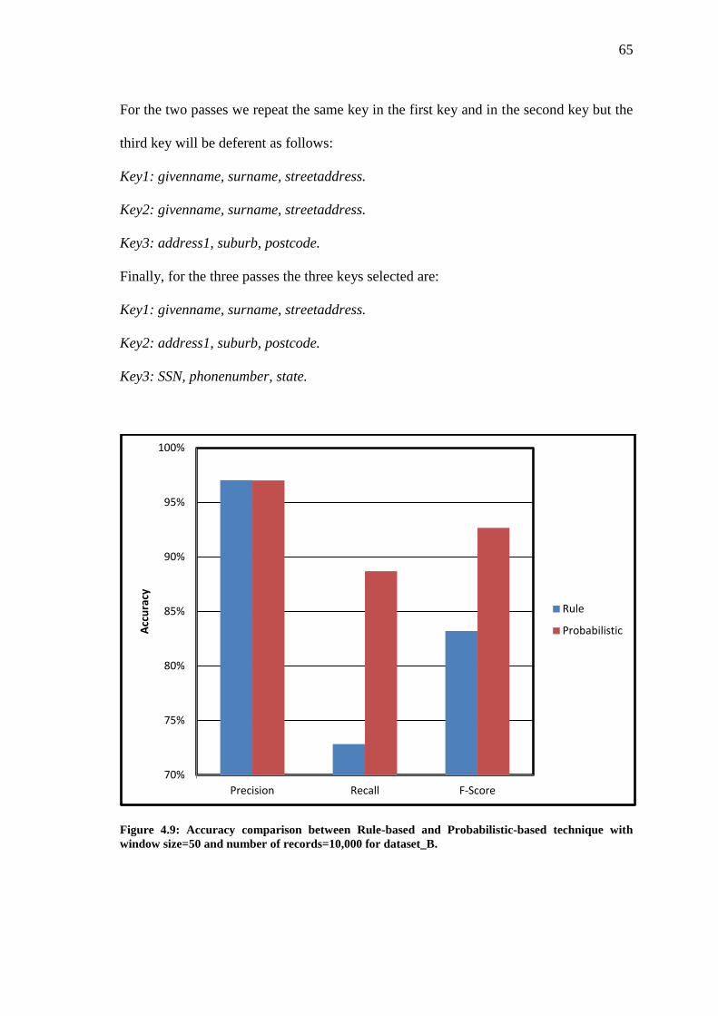
65

For the two passes we repeat the same key in the first key and in the second key but the

third key will be deferent as follows:

Key1: givenname, surname, streetaddress.

Key2: givenname, surname, streetaddress.

Key3: address1, suburb, postcode.

Finally, for the three passes the three keys selected are:

Key1: givenname, surname, streetaddress.

Key2: address1, suburb, postcode.

Key3: SSN, phonenumber, state.

Figure 4.9: Accuracy comparison between Rule-based and Probabilistic-based technique with

window size=50 and number of records=10,000 for dataset_B.

70%

75%

80%

85%

90%

95%

100%

Precision Recall F-Score

Acc

ura

cy

Rule

Probabilistic

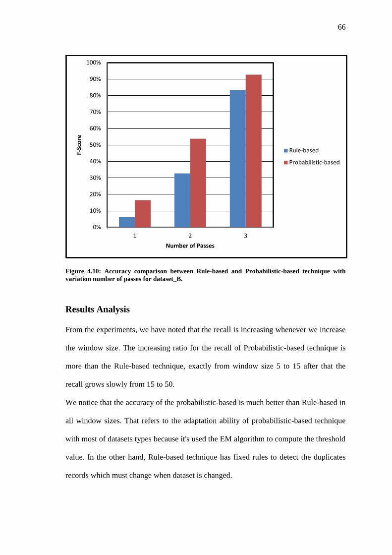
66

Figure 4.10: Accuracy comparison between Rule-based and Probabilistic-based technique with

variation number of passes for dataset_B.

Results Analysis

From the experiments, we have noted that the recall is increasing whenever we increase

the window size. The increasing ratio for the recall of Probabilistic-based technique is

more than the Rule-based technique, exactly from window size 5 to 15 after that the

recall grows slowly from 15 to 50.

We notice that the accuracy of the probabilistic-based is much better than Rule-based in

all window sizes. That refers to the adaptation ability of probabilistic-based technique

with most of datasets types because it's used the EM algorithm to compute the threshold

value. In the other hand, Rule-based technique has fixed rules to detect the duplicates

records which must change when dataset is changed.

0%

10%

20%

30%

40%

50%

60%

70%

80%

90%

100%

1 2 3

F-Sc

ore

Number of Passes

Rule-based

Probabilistic-based

67

Comparing the results for the precision, we have noted that precision stays stable when

increasing the window size with insignificant change because of the stability of

the number of false positive.

In general recall decreased whenever dataset size increases for both techniques with

better results for Probabilistic-based

For the Rule-based technique, the decreasing is almost linear because it's not involved

with dataset size as the duplication percentage in the dataset. The precision for both

techniques is almost fixed among the increasing size of the dataset.

We measure the time efficiency for both techniques; processing time collected during

the tests shows clearly that Probabilistic-based technique is having the higher

processing time.

The F-Score is computed from the Recall and Precision to get a good view of the two

techniques. This shows that the Probabilistic-based technique has higher F-Score with

92.66% than Rule-based technique with 83.20%.

At last, we notice that increasing the number of passes will affect positively the

accuracy of the system. The good selection of the pass key will effect on the F-Score

value. The experiments show that Probabilistic-based technique outperforms the Rule-

based technique on dataset_B.

68

Chapter 5

Conclusion and Future Work

This chapter summarizes the conclusions we have achieved in this thesis and discussing

of the possible future works that can further extend or improve our work.

5.1 Conclusion

The purpose of duplicate record detection is finding multiple representations of the

same real world object. This problem is compromised of two difficult problems: First

finding an adequate similarity measure to decide upon duplicity, and second finding an

efficient algorithm to detect as many duplicates as possible.

In this study we have presented a generic framework for detecting the duplicate records

in a database. Our framework consists of two decision models; Rule-based model that

uses domain-knowledge to define rules to identify duplicate and non-duplicates, and

Probabilistic-based model that employs the EM algorithm to find likelihood ratio and

determine according to it the duplicates or non-duplicates. We have clarified the

variation between them with using the same blocking technique (Sorted-neighborhood)

and similarity function (Q-gram), and we have experimentally compared their

performance and efficiency.

We have conducted various experiments on a synthetic dataset to evaluate our

implementation of both Rule-based and Probabilistic-based technique. The experiments

confirmed that Probabilistic-based technique outperformed the Rule-based techniques

when changing the window size of the sorted neighborhood technique, increasing

dataset size, and changing the sorting keys. Rule-based technique acts better than

Probabilistic-based technique when comparing them in term of time efficiency.

69

In our study we used high threshold values to decrease the false positives, meanwhile

choosing appropriate threshold value refer to the dataset that is evaluated. For example,

if the database contains patient's information like our datasets it is recommended to use

high threshold to avoid matching two different persons. On the other hand, credit-rating

agencies database concern with detecting duplicates even if they not so in this case low

threshold values are needed.

5.2 Future Work

As the database systems become more and more common place, and with the

accumulating vast amounts of errors on a daily basis, we believe that there is still room

for substantial improvement in the current state-of-the-art. There are a number of key

challenges that are important to address in future.

The experiment was done using synthetic data set and needed to be confirmed with

different data sets, with real-world datasets and with large-scale datasets (millions of

records) in order to verify the effectiveness and efficiency of the proposed decision

models.

Minimizing the manual insertion of parameters used by the system, and experts

interference by design the appropriate rules. That can be done by using the EM

algorithm with the Rule-based to determine the significant attributes which could be

used in the rules designing.

Improve the selection of blocking key value which is used to sort the dataset using

different techniques such as phonetic coding.

Our work in this thesis in terms of performance measurements has focused on

processing time as a major measurement where in the future we can address other

needed criteria such as the effect on systems resources such as memory and disk usage.

70

Finally, we need to have a comprehensive framework that can determine which decision

model is better with specific dataset, and that requires evaluating and comparing other

decision models that we did not mention in this study such as supervised learning and

semi-supervised learning techniques.

71

REFERENCES

Alnoory, M., (2011): Performance Evaluation of Similarity Functions for Duplicate

Record Detection, Master Thesis, Middle East University, Jordan.

Baxter, R., Christen, P. & Churches, T., (2003): A Comparison of Fast Blocking

Methods for Record Linkage, ACM SIGKDD Workshop on Data Cleaning, Record

Linkage and Object Consolidation, Washington DC, pp. 25-27.

Bertolazzi, P., DeSantis, L., & Scannapieco, M., (2003): Automatic Record Matching in

Cooperative Information Systems, Proceedings of the Workshop on Data Quality in

Cooperative Information Systems (ICDT'03).

Bleiholder, J., & Naumann, F., (2008): Data Fusion, Data Fusion Journal: ACM

Computing Surveys, Vol. 41, No. 1, Article 1.

Christen, P., (2006): A Comparison of Personal Name Matching: Techniques and

Practical Issues. Joint Computer Science Technical Report Series, September. Tr-Cs-06-

02, Department Of Computer Science, Computer Sciences Laboratory Research School

Of Information Sciences And Engineering, The Australian National University.

Christen, P., (2007): Improving data linkage and deduplication quality through nearest-

neighbor based blocking. Proceeding of thirteenth ACM SIGKDD International

Conference on Knowledge Discovery and Data Mining (KDD'07).

Christen, P., & Churches, T., (2005): Febrl: Freely extensible biomedical record linkage

manual.

Dempster, A., Laird, N., & Rubin, D., (1977): Maximum likelihood from incomplete

data via the em algorithm. Journal of the Royal Statistical Society, 39:1–38.

Draisbach, U. & Naumann, F., (2009): Comparison and Generalization of Blocking and

Windowing Algorithms for Duplicate Detection, Proceedings of QDB 2009 Workshop

at VLDB.

Elmagarmid, A., Ipeirotis, P. & Verykios, V., (2007): Duplicate Record Detection: A

Survey, IEEE Transactions on Knowledge and Data Engineering, VOL. 19, NO. 1.

Fellegi, I., & Sunter, A., (1969): A theory for record linkage. Journal of the American

Statistical Association, 64:1183–1210.

Gu, L., Baxter, R., Vickers, D., & Rainsford, C., (2003): Record Linkage: Current

Practice and Future Directions: Technical Report 03/83, CSIRO Mathematical and

Information Sciences.

Hernández, M., & Stolfo, S., (1998): Real-world Data is Dirty: Data Cleansing and The

Merge/Purge Problem, Data Mining and Knowledge Discovery, Volume 2, Issue 1,

Pages: 9-37.

72

Innerhofer-Oberperfler, R., (2004): Using Approximate String Matching, Techniques to

Join Street Names of Residential Addresses, Bachelor Thesis, Academic Year

2003/2004 1st Graduate Session.

Jaro, M., (1989): Advances in Record-linkage Methodology as Applied to Matching the

1985 census of Tampa, Florida. Journal of the American Statistical Association, 89:

414-420.

Lim, E., Srivastava, J., & Richardson, J., (1993): Entity identification in database

integration. In Proc. Ninth IEEE Int’l Conf. Data Eng. (ICDE ’93), pages 294–301.

Naumann, F., & Herrschel, M., (2010): An Introduction to Duplicate Detection. USA.

Morgan & Claypool Publishers.

Newcombe, H., Kennedy, J., Axford, S., & James, A., (1959): Automatic linkage of

vital records. Science. 130 (3381). pp. 954–959.

Scannapieco, M., Missier, P., & Batini, C., (2005): Data Quality at a Glance: Databank

Spektrum Journal issue 14.

Tamilselvi, J., & Saravanan, V., (2009): Detection and Elimination of Duplicate Data

Using Token-Based Method for a Data Warehouse: A Clustering Based Approach,

International Journal of Dynamics of Fluids, ISSN 0973-1784 Volume 5, Number 2, pp.

145–164.

Ukkonen, E., (1992): Approximate string-matching with Q-grams and maximal

matches, Theoretical Computer Science, Volume 92, Issue 1, Selected papers of the

Combinatorial Pattern Matching School, Pages: 191 - 211.

Wang, X., (2008): Matching records in multiple databases using a hybridization of

several technologies, Dissertation. Department of Industrial Engineering. University of

Louisville, KY, USA.

Wang, Y., & Madnick, S., (1989): The inter-database instance identification problem in

integrating autonomous systems. In Proc. fifth IEEE Int’l Conf. data Eng. (ICDE ’89).

Winkler, W., (1993): Improved decision rules in the fellegi-sunter model of record

linkage. In Technical Report Statistical Research Report Series RR93/12, US Bureau of

the Census, Washington.

Winkler, W., (2002): Methods for Record Linkage and Bayesian Networks. In

Technical Report Statistical Research Report Series RRS2002/05, US Bureau of the

Census, Washington, D.C.

Yan, S., Lee, D., Kan, M., & Giles, C., (2007): Adaptive Sorted Neighborhood Methods

for Efficient Record Linkage. International conference on digital libraries JCDL'07,

Vancouver, British Columbia, Canada.

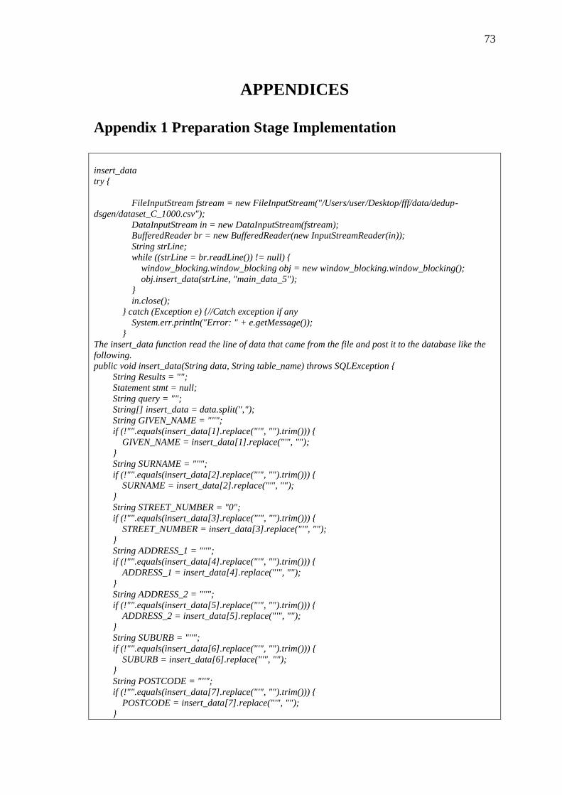
73

APPENDICES

Appendix 1 Preparation Stage Implementation

insert_data

try {

FileInputStream fstream = new FileInputStream("/Users/user/Desktop/fff/data/dedup-

dsgen/dataset_C_1000.csv");

DataInputStream in = new DataInputStream(fstream);

BufferedReader br = new BufferedReader(new InputStreamReader(in));

String strLine;

while ((strLine = br.readLine()) != null) {

window_blocking.window_blocking obj = new window_blocking.window_blocking();

obj.insert_data(strLine, "main_data_5");

}

in.close();

} catch (Exception e) {//Catch exception if any

System.err.println("Error: " + e.getMessage());

}

The insert_data function read the line of data that came from the file and post it to the database like the

following.

public void insert_data(String data, String table_name) throws SQLException {

String Results = "";

Statement stmt = null;

String query = "";

String[] insert_data = data.split(",");

String GIVEN_NAME = "''";

if (!"".equals(insert_data[1].replace("'", "").trim())) {

GIVEN_NAME = insert_data[1].replace("'", "");

}

String SURNAME = "''";

if (!"".equals(insert_data[2].replace("'", "").trim())) {

SURNAME = insert_data[2].replace("'", "");

}

String STREET_NUMBER = "0";

if (!"".equals(insert_data[3].replace("'", "").trim())) {

STREET_NUMBER = insert_data[3].replace("'", "");

}

String ADDRESS_1 = "''";

if (!"".equals(insert_data[4].replace("'", "").trim())) {

ADDRESS_1 = insert_data[4].replace("'", "");

}

String ADDRESS_2 = "''";

if (!"".equals(insert_data[5].replace("'", "").trim())) {

ADDRESS_2 = insert_data[5].replace("'", "");

}

String SUBURB = "''";

if (!"".equals(insert_data[6].replace("'", "").trim())) {

SUBURB = insert_data[6].replace("'", "");

}

String POSTCODE = "''";

if (!"".equals(insert_data[7].replace("'", "").trim())) {

POSTCODE = insert_data[7].replace("'", "");

}

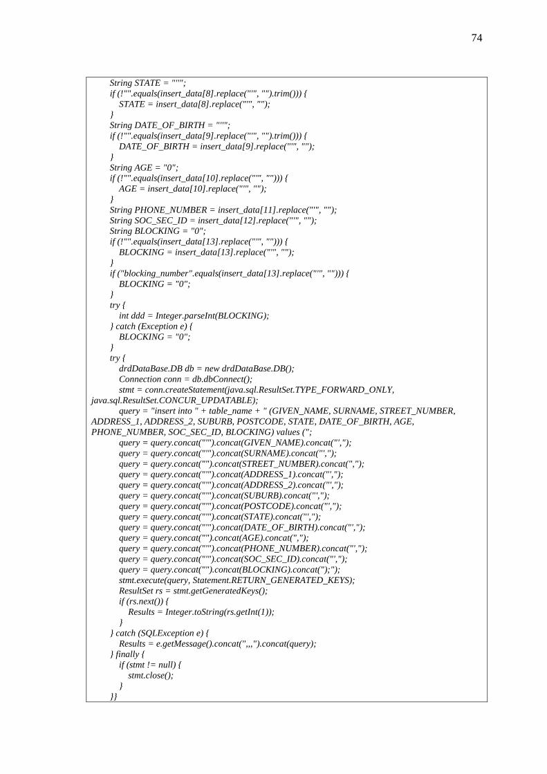
74

String STATE = "''";

if (!"".equals(insert_data[8].replace("'", "").trim())) {

STATE = insert_data[8].replace("'", "");

}

String DATE_OF_BIRTH = "''";

if (!"".equals(insert_data[9].replace("'", "").trim())) {

DATE_OF_BIRTH = insert_data[9].replace("'", "");

}

String AGE = "0";

if (!"".equals(insert_data[10].replace("'", ""))) {

AGE = insert_data[10].replace("'", "");

}

String PHONE_NUMBER = insert_data[11].replace("'", "");

String SOC_SEC_ID = insert_data[12].replace("'", "");

String BLOCKING = "0";

if (!"".equals(insert_data[13].replace("'", ""))) {

BLOCKING = insert_data[13].replace("'", "");

}

if ("blocking_number".equals(insert_data[13].replace("'", ""))) {

BLOCKING = "0";

}

try {

int ddd = Integer.parseInt(BLOCKING);

} catch (Exception e) {

BLOCKING = "0";

}

try {

drdDataBase.DB db = new drdDataBase.DB();

Connection conn = db.dbConnect();

stmt = conn.createStatement(java.sql.ResultSet.TYPE_FORWARD_ONLY,

java.sql.ResultSet.CONCUR_UPDATABLE);

query = "insert into " + table_name + " (GIVEN_NAME, SURNAME, STREET_NUMBER,

ADDRESS_1, ADDRESS_2, SUBURB, POSTCODE, STATE, DATE_OF_BIRTH, AGE,

PHONE_NUMBER, SOC_SEC_ID, BLOCKING) values (";

query = query.concat("'").concat(GIVEN_NAME).concat("',");

query = query.concat("'").concat(SURNAME).concat("',");

query = query.concat("").concat(STREET_NUMBER).concat(",");

query = query.concat("'").concat(ADDRESS_1).concat("',");

query = query.concat("'").concat(ADDRESS_2).concat("',");

query = query.concat("'").concat(SUBURB).concat("',");

query = query.concat("'").concat(POSTCODE).concat("',");

query = query.concat("'").concat(STATE).concat("',");

query = query.concat("'").concat(DATE_OF_BIRTH).concat("',");

query = query.concat("").concat(AGE).concat(",");

query = query.concat("'").concat(PHONE_NUMBER).concat("',");

query = query.concat("'").concat(SOC_SEC_ID).concat("',");

query = query.concat("").concat(BLOCKING).concat(");");

stmt.execute(query, Statement.RETURN_GENERATED_KEYS);

ResultSet rs = stmt.getGeneratedKeys();

if (rs.next()) {

Results = Integer.toString(rs.getInt(1));

}

} catch (SQLException e) {

Results = e.getMessage().concat(",,,").concat(query);

} finally {

if (stmt != null) {

stmt.close();

}

}}

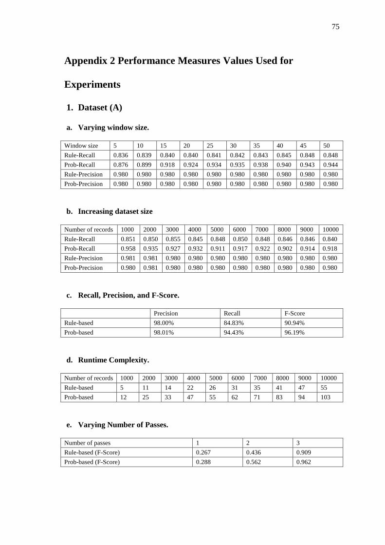
75

Appendix 2 Performance Measures Values Used for

Experiments

1. Dataset (A)

a. Varying window size.

Window size 5 10 15 20 25 30 35 40 45 50

Rule-Recall 0.836 0.839 0.840 0.840 0.841 0.842 0.843 0.845 0.848 0.848

Prob-Recall 0.876 0.899 0.918 0.924 0.934 0.935 0.938 0.940 0.943 0.944

Rule-Precision 0.980 0.980 0.980 0.980 0.980 0.980 0.980 0.980 0.980 0.980

Prob-Precision 0.980 0.980 0.980 0.980 0.980 0.980 0.980 0.980 0.980 0.980

b. Increasing dataset size

Number of records 1000 2000 3000 4000 5000 6000 7000 8000 9000 10000

Rule-Recall 0.851 0.850 0.855 0.845 0.848 0.850 0.848 0.846 0.846 0.840

Prob-Recall 0.958 0.935 0.927 0.932 0.911 0.917 0.922 0.902 0.914 0.918

Rule-Precision 0.981 0.981 0.980 0.980 0.980 0.980 0.980 0.980 0.980 0.980

Prob-Precision 0.980 0.981 0.980 0.980 0.980 0.980 0.980 0.980 0.980 0.980

c. Recall, Precision, and F-Score.

Precision Recall F-Score

Rule-based 98.00% 84.83% 90.94%

Prob-based 98.01% 94.43% 96.19%

d. Runtime Complexity.

Number of records 1000 2000 3000 4000 5000 6000 7000 8000 9000 10000

Rule-based 5 11 14 22 26 31 35 41 47 55

Prob-based 12 25 33 47 55 62 71 83 94 103

e. Varying Number of Passes.

Number of passes 1 2 3

Rule-based (F-Score) 0.267 0.436 0.909

Prob-based (F-Score) 0.288 0.562 0.962

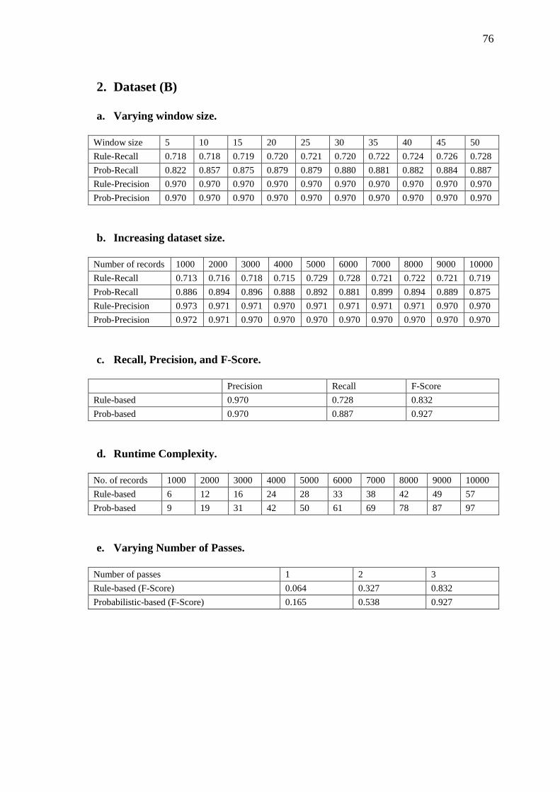
76

2. Dataset (B)

a. Varying window size.

Window size 5 10 15 20 25 30 35 40 45 50

Rule-Recall 0.718 0.718 0.719 0.720 0.721 0.720 0.722 0.724 0.726 0.728

Prob-Recall 0.822 0.857 0.875 0.879 0.879 0.880 0.881 0.882 0.884 0.887

Rule-Precision 0.970 0.970 0.970 0.970 0.970 0.970 0.970 0.970 0.970 0.970

Prob-Precision 0.970 0.970 0.970 0.970 0.970 0.970 0.970 0.970 0.970 0.970

b. Increasing dataset size.

Number of records 1000 2000 3000 4000 5000 6000 7000 8000 9000 10000

Rule-Recall 0.713 0.716 0.718 0.715 0.729 0.728 0.721 0.722 0.721 0.719

Prob-Recall 0.886 0.894 0.896 0.888 0.892 0.881 0.899 0.894 0.889 0.875

Rule-Precision 0.973 0.971 0.971 0.970 0.971 0.971 0.971 0.971 0.970 0.970

Prob-Precision 0.972 0.971 0.970 0.970 0.970 0.970 0.970 0.970 0.970 0.970

c. Recall, Precision, and F-Score.

Precision Recall F-Score

Rule-based 0.970 0.728 0.832

Prob-based 0.970 0.887 0.927

d. Runtime Complexity.

No. of records 1000 2000 3000 4000 5000 6000 7000 8000 9000 10000

Rule-based 6 12 16 24 28 33 38 42 49 57

Prob-based 9 19 31 42 50 61 69 78 87 97

e. Varying Number of Passes.

Number of passes 1 2 3

Rule-based (F-Score) 0.064 0.327 0.832

Probabilistic-based (F-Score) 0.165 0.538 0.927