A Comparative Study of DOA Estimation Algorithms With Application to Tracking Using Kalman Filter
17
Signal & Image Processing : An International Journal (SIPIJ) Vol.6, No.6, December 2015 DOI : 10.5121/sipij.2015.6602 13 A COMPARATIVE STUDY OF DOA ESTIMATION ALGORITHMS WITH APPLICATION TO TRACKING USING KALMAN FILTER Venu Madhava M 1 , Jagadeesha S N 1 , and Yerriswamy T 2 1 Department of Computer Science and Engineering, JNN College of Engineering, Shimoga 2 Department of Computer Science and Engineering, KLE Institute of Technology, Hubli ABSTRACT Tracking the Direction of Arrival (DOA) Estimation of a moving source is an important and challenging task in the field of navigation, RADAR, SONAR, Wireless Sensor Networks (WSNs) etc. Tracking is carried out starting from the estimation of DOA, considering the estimated DOA as an initial value, the Kalman Filter (KF) algorithm is used to track the moving source based on the motion model which governs the motion of the source. This comparative study deals with analysis, significance of Non-coherent, Narrowband DOA (Direction of Arrival) Estimation Algorithms in perception to tracking. The DOA estimation algorithms Multiple Signal Classification (MUSIC), Root-MUSIC& Estimation of Signal Parameters via Rotational Invariance Technique (ESPRIT) are considered for the purpose of the study, a comparison in terms of optimality with respect to Signal to Noise Ratio (SNR), number of snapshots and number of Antenna elements used and Computational complexity is drawn between the chosen algorithms resulting in an optimum DOA estimate. The optimum DOA Estimate is taken as an initial value for the Kalman filter tracking algorithm. The Kalman filter algorithm is used to track the optimum DOA Estimate. KEYWORDS Direction of arrival (DOA), MUSIC, Root-MUSIC, ESPRIT, Tracking, Kalman filter. 1. INTRODUCTION The Estimation of Direction of Arrival (DOA) and its tracking, is the most significant area of array signal processing and finds its applications in the fields of RADAR, SONAR, Wireless Sensor Networks (WSN),Seismology etc. [1]. Tracking the DOA Estimation is estimating the value of DOA of the signals from various sources impinging on the array of sensors at each scanning instant of time [2]. The tracking is performed in order to get correlated estimates at different instants of time. The correlation between the data is also known as data association or estimate association. In the first step, the plane wave fronts from far field are considered to be falling on the Uniform Linear Array (ULA) [11]. A particular number of snapshots are collected and the DOA is estimated using techniques like Multiple SIgnal Classification (MUSIC), Root- MUSIC and Estimation of Signal Parameters via Rotational Invariance Technique (ESPRIT). All the three algorithms estimate the DOA of the sources which are stationary but the estimation of
description
Tracking the Direction of Arrival (DOA) Estimation of a moving source is an important and challenging task in the field of navigation, RADAR, SONAR, Wireless Sensor Networks (WSNs) etc. Tracking is carried out starting from the estimation of DOA, considering the estimated DOA as an initial value, the Kalman Filter (KF) algorithm is used to track the moving source based on the motion model which governs the motion of the source. This comparative study deals with analysis, significance of Non-coherent, Narrowband DOA (Direction of Arrival) Estimation Algorithms in perception to tracking. The DOA estimation algorithms Multiple Signal Classification (MUSIC), Root-MUSIC& Estimation of Signal Parameters via Rotational Invariance Technique (ESPRIT) are considered for the purpose of the study, a comparison in terms of optimality with respect to Signal to Noise Ratio (SNR), number of snapshots and number of Antenna elements used and Computational complexity is drawn between the chosen algorithms resulting in an optimum DOA estimate. The optimum DOA Estimate is taken as an initial value for the Kalman filter tracking algorithm. The Kalman filter algorithm is used to track the optimum DOA Estimate.
Transcript of A Comparative Study of DOA Estimation Algorithms With Application to Tracking Using Kalman Filter
Signal & Image Processing : An International Journal (SIPIJ) Vol.6, No.6, December 2015
DOI : 10.5121/sipij.2015.6602 13
A COMPARATIVE STUDY OF DOA ESTIMATION
ALGORITHMS WITH APPLICATION TO
TRACKING USING KALMAN FILTER
Venu Madhava M1, Jagadeesha S N
1, and Yerriswamy T
2
1Department of Computer Science and Engineering,
JNN College of Engineering, Shimoga 2Department of Computer Science and Engineering,
KLE Institute of Technology, Hubli
ABSTRACT Tracking the Direction of Arrival (DOA) Estimation of a moving source is an important and challenging
task in the field of navigation, RADAR, SONAR, Wireless Sensor Networks (WSNs) etc. Tracking is carried
out starting from the estimation of DOA, considering the estimated DOA as an initial value, the Kalman
Filter (KF) algorithm is used to track the moving source based on the motion model which governs the
motion of the source. This comparative study deals with analysis, significance of Non-coherent,
Narrowband DOA (Direction of Arrival) Estimation Algorithms in perception to tracking. The DOA
estimation algorithms Multiple Signal Classification (MUSIC), Root-MUSIC& Estimation of Signal
Parameters via Rotational Invariance Technique (ESPRIT) are considered for the purpose of the study, a
comparison in terms of optimality with respect to Signal to Noise Ratio (SNR), number of snapshots and
number of Antenna elements used and Computational complexity is drawn between the chosen algorithms
resulting in an optimum DOA estimate. The optimum DOA Estimate is taken as an initial value for the
Kalman filter tracking algorithm. The Kalman filter algorithm is used to track the optimum DOA Estimate.
KEYWORDS Direction of arrival (DOA), MUSIC, Root-MUSIC, ESPRIT, Tracking, Kalman filter.
1. INTRODUCTION The Estimation of Direction of Arrival (DOA) and its tracking, is the most significant area of
array signal processing and finds its applications in the fields of RADAR, SONAR, Wireless
Sensor Networks (WSN),Seismology etc. [1]. Tracking the DOA Estimation is estimating the
value of DOA of the signals from various sources impinging on the array of sensors at each
scanning instant of time [2]. The tracking is performed in order to get correlated estimates at
different instants of time. The correlation between the data is also known as data association or
estimate association. In the first step, the plane wave fronts from far field are considered to be
falling on the Uniform Linear Array (ULA) [11]. A particular number of snapshots are collected
and the DOA is estimated using techniques like Multiple SIgnal Classification (MUSIC), Root-
MUSIC and Estimation of Signal Parameters via Rotational Invariance Technique (ESPRIT). All
the three algorithms estimate the DOA of the sources which are stationary but the estimation of
Signal & Image Processing : An International Journal (SIPIJ) Vol.6, No.6, December 2015
14
DOA of the moving source is an important problem. In order to estimate the DOA of the moving
target, the Estimated DOA will Act as an initial value to the Kalman filter algorithm and the
Kalman filter algorithm tracks the DOA at each scanning instant of time based on the target
motion model [2] [16].Unlike, this method ,MUSIC, Root-MUSIC or ESPRIT can be used to
estimate the instantaneous DOA estimate provided that there is no requirement of data
association and the process will be slow. In the present study, we draw brief comparisons among
the three most used DOA estimation algorithms viz MUSIC [3], Root-MUSIC [4], ESPRIT [5].
These algorithms are also known as high resolution DOA Estimation algorithms. It is assumed
that the Signals are non-coherent, narrowband sources. The DOA Estimation is performed in
multiple source scenarios and tracking is performed on single source.
2. BACKGROUND AND FRAMEWORK
Estimating and tracking the signal parameters viz Time, Frequency, Phase and DOA are
interesting and find applications in areas of RADAR, SONAR, Seismology, Air Traffic Control
etc. There are various types of estimation techniques such as classical techniques, Beam forming,
Spectral based and parametric approaches[6][13].
The Maximum Likelihood (ML) DOA estimation technique [10] [13] was originally developed
by R. A. Fisher in 1920‟s. Under the suitable assumptions, it estimates the DOA of the incoming
signal with the help of maximizing the log-likelihood function of the sampled data sequences
coming from a direction.
In the beamforming technique [13], the array is steered in one direction and the output power is
measured. We observe maximum power when steered direction and DOA of signal are in line.
These techniques find out the output of the array by linear combination of the data received with
a weight vector. If the array weight vector is used then it is known as conventional beam forming
technique.
In subspace based techniques for DOA Estimation such as MUSIC [3], we get a spectrum like
function of interested parameters, whose distinct peaks are the interested estimated parameters.
Although MUSIC algorithm being robust and computationally less complex, it needs a search
algorithm to identify the largest of the peaks. In Root-MUSIC [4] & ESPRIT [5], a search over
all the parameters of interest is carried out to get more accurate estimates being computationally
expensive. In order to track the parameters, we have adaptive algorithms. These are in turn
divided mainly into two types; Least Mean Square (LMS)[2][6] are the types of algorithms which
converge at slow rates dependent on the number of step sizes and Recursive Least Squares
(RLS)[2][6] are the types of algorithms which converge much quickly compared to the former
type of algorithms. In the present literature, one of the later (RLS) type of algorithm viz Kalman
filter is used to track the DOA Estimation of the moving target. The Kalman Filter algorithms
proposed by R.E.Kalman in 1960 [16] are basic type of tracking algorithms which consider the
state-space model of the moving target to estimate the components of motion. This section gives
out the necessary framework to perform the tracking operation of the optimum DOA Estimate.
2.1 System model
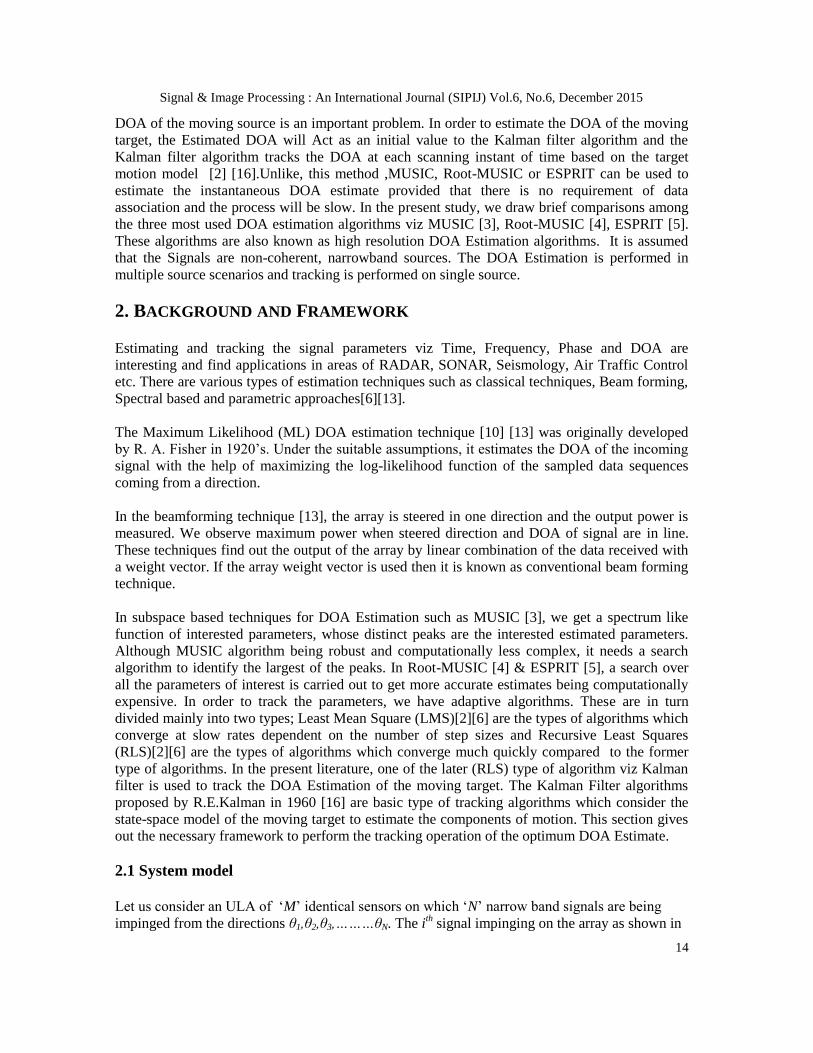
Let us consider an ULA of „M‟ identical sensors on which „N‟ narrow band signals are being
impinged from the directions θ1,θ2,θ3,………θN. The ith signal impinging on the array as shown in
Signal & Image Processing : An International Journal (SIPIJ) Vol.6, No.6, December 2015
15
the Fig 1 is given by
( )( ) 1,2,3, ,ij t
i iS t S e i N
(1)
Where, Si, ω, ϕi are the amplitude, frequency and phase of the signals of three parameters, phase
ϕ is considered to be a uniformly distributed random variable. Let us define a column vector S(t)
as
1 2( ) [ ( ), ( ),......... ( )]T
NS t S t S t S t (2)
Where „T‟ denotes Transpose.
Fig 1: Illustration of the DOA Estimation Model
The direction vector of the ith source is given by
( 1) ( 1)1 2( )( ) ( )
( ) [1, , ,............., ] 1,2,3 ,M M ii i i ijj j T
ia e e e i N
(3)
Where, ( 1) sin 1,2,3m i
dm m M
c
(4)
d is the inter element spacing , c being the propagation velocity of the plane wave front. The inter
element spacing is assumed to be less than or equal to half the wavelength of the signal
impinging. This assumption is made in order to avoid spatial aliasing.
Substitute (4) in (3) and replacing ω=2πfc , we get the array response vector for the ULA and it is
given by
2 2sin( ) ( 1) sin( )
( ) [1, ,............, ] 1,2,3 ,i ij d j M d
T
ia e e i N
(5)
Where, fc is the carrier frequency and λω is the wavelength and they are related by fc=c/ λω
At the mth element, the received signal is given by

Signal & Image Processing : An International Journal (SIPIJ) Vol.6, No.6, December 2015
16
1
2( ) ( )exp( ( 1) sin( )) 1,2,3, ,m i
dx t x t j m i M
c
(6)
Where x1(t) is the received signal vector at the first element of the ULA. The direction vector
matrix is given by
1 2[ ( ), ( ),..... ( )]NA a a a (7)
Assuming white Gaussian noise ni(t) at all the elements, the received signal at the output of the
array is given by,
1 2 3( ) [ ( ), ( ), ( ),....., ( )]T
Mx t x t x t x t x t
( ) ( )AS t n t (8)
Where, A is a MxN direction or steering vector matrix. If we discretize the above, the input
signals of the array are discrete in time and the output of the array is given by
( ) ( ) ( ) 1,2,3, ,X k AS k n k k K (9)
Where, k is the sample instance and K is the number of snapshots. The parameters of the signal
from the source which we are interested in are spatial in nature. Hence they require spatial
correlation matrix.
2
2
{ ( ) ( )} [ ( ) ( )]H H H
H
S
R E X k X k AE S k S k A I
AR A I
(10)
Where, Rs is the signal correlation matrix, 2 is the Noise variance and I is the identity matrix.
Practically, the correlation matrix [7] is unknown and it has to be estimated from the array output
data. If the underlying processes are ergodic, then the statistical expectation can be replaced by
time average.
Let us consider that, ( )x k is the signal corrupted by noise having K snapshots are received at the
output of the array. The received signal ( )x k is denoted by X which is also known as stacked data
matrix. The similar stacking is applied to pure signal vector S(k) and the noise vector n(k) as S
and N respectively. Equation (9) can be written as
X AS N (11)
Where, X is the received noise corrupted signal matrix of size MxK, A is the direction or steering
vector matrix of size MxN, S is the signal matrix of size NxK, N is the additive white Gaussian
matrix of size MxK.
The ensemble correlation matrix estimate is computed by
1
1 1ˆ ( ) ( ) [ ]K
H H
k
R x k x k XXK K
(12)

Signal & Image Processing : An International Journal (SIPIJ) Vol.6, No.6, December 2015
17
2.2. Subspace based techniques
The subspace based methods of DOA estimation use the estimated correlation matrix,
decomposing it and carrying out the analysis on the decomposition. These techniques were
started from a paper published by V.T. Pisarenko [14], later tremendously progressed by the
introduction of MUSIC proposed by R.O.Schmidt and followed by ESPRIT by Roy and Kailath.
These techniques use the Eigen decomposition of the estimated correlation matrix into signal and
noise subspaces.
The array output correlation matrix is given by
2ˆ [ ]H HR AE SS A I
2H
SAR A I (13)
Where Rs is the signal correlation matrix 2 is the noise variance and I is the identity matrix. The
correlation matrix of (13) is decomposed using Eigen Value Decomposition (EVD) to obtain
ˆ HR V V (14)
Where, V is the unitary matrix of Eigen vectors of R as columns, is the diagonal matrix of
Eigen values of R. In the present literature, we assume that the sources are uncorrelated and hence
the rank of the correlation matrix R is M and that of RS is N.
Eigen values of R: λ1˃λ2˃……˃λM
Eigen values of signal subspace RS: λ1˃λ2˃……˃λN.
Remaining (M-N) Eigen values corresponds to noise subspace. The columns of V are orthogonal.
Hence, the correlation matrix can also be decomposed as
ˆ HR V V
H H
S S n n nV V V V (15)
Where SV are signal Eigen vectors, S are signal Eigen values both span the signal subspace ES.
nV and n are noise Eigen vectors and Eigen values respectively spanning the complement of
signal subspace called noise subspace En.
2.2.1 MUSIC
MUSIC Stands for Multiple SIgnal Classification and it is a high resolution DOA estimation
algorithm. It gives the estimate of DOA of signals as well as the estimate of the number of
signals. In this algorithm, the estimation of DOA can be carried out by using one of the subspaces
either noise or signal. The steps followed to estimate DOA using MUSIC are as follows
Step 1: Estimate the correlation Matrix R̂ from the equation
1ˆ [ ]HR XXK
(16)

Signal & Image Processing : An International Journal (SIPIJ) Vol.6, No.6, December 2015
18
Step 2: Find the Eigen decomposition of the estimated correlation matrix using the following
equation
ˆ ˆ ˆ ˆ HR V V (17)
Step 3: Find the noise decomposition of V̂ matrix to find the span of noise subspace nV
Step 4: Plot the MUSIC function MusicP as a function of θ
Step 5: The M Signal directions are the M largest peaks of the plot.
The MUSIC Algorithm along with the required number of operations are summarised in the table
below Table 1: Summary of the MUSIC Algorithm
Input to the algorithm θ, a(θ)
No Operation performed Complexity
1 Estimation of Correlation Matrix KM2
2 Eigen decomposition of correlation Matrix O(M3)
3 Selecting the (N-M) Eigen pair to obtain Noise subspace
((M-N)MK3) 4 Plotting the Music function and identifying „M‟ Large peaks
of the plot
Total KM2+O(M
3)+((M-N)MK
3)
From the Table 1, it has been observed that, the MUSIC algorithm is having the computational
complexity of the order of „M3‟. Search algorithm is needed to decide the largest „N‟ peaks. This
increases the computational complexity.
2.2.2 Root-MUSIC
In order to overcome the necessity of comprehensive search algorithm to locate largest „N‟ peaks
in the MUSIC algorithm, a new algorithm which gives the results numerically has been
developed. The algorithm is known as Root-MUSIC is a model based parametric estimation
technique. It is also a polynomial rooting version of the MUSIC algorithm. The algorithm
operates in the following steps.
Step 1: Estimate the Correlation Matrix „R‟ from the equation
1ˆ [ ]HR XXK
(19)
Step 2: Find the Eigen decomposition of the estimated correlation matrix using the following
equation
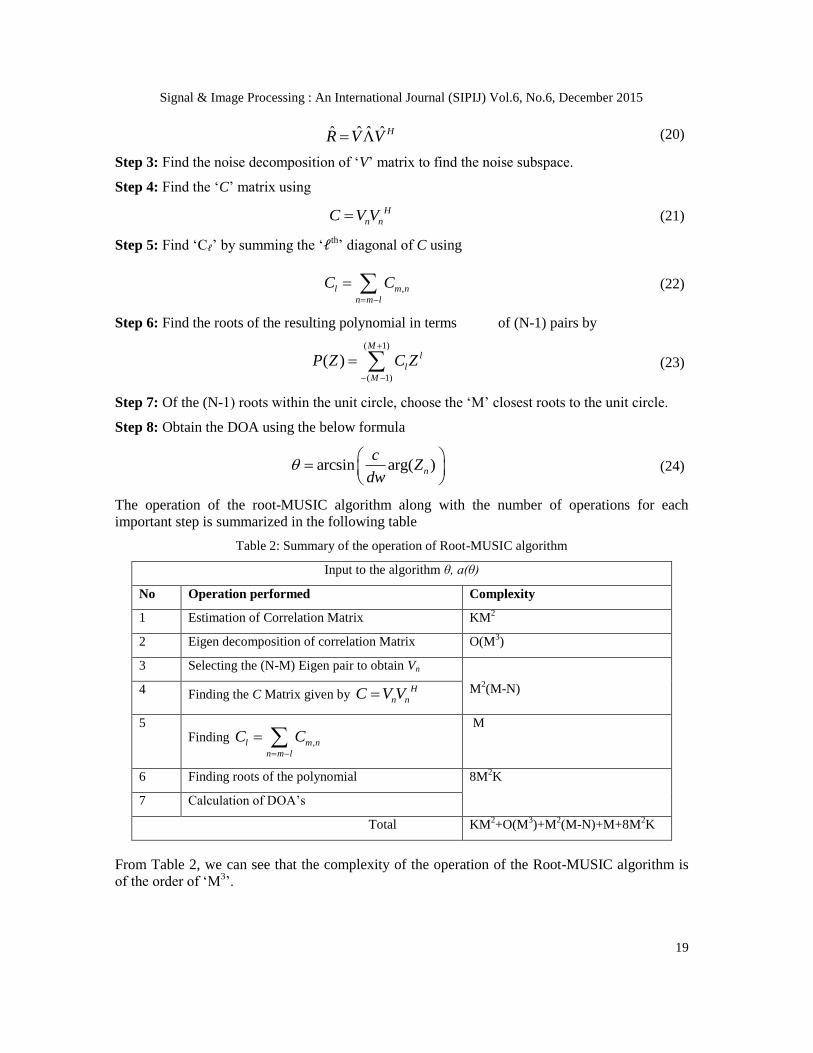
Signal & Image Processing : An International Journal (SIPIJ) Vol.6, No.6, December 2015
19
ˆ ˆ ˆ ˆ HR V V (20)
Step 3: Find the noise decomposition of „V‟ matrix to find the noise subspace.
Step 4: Find the „C‟ matrix using
H
n nC V V (21)
Step 5: Find „C𝓁‟ by summing the „𝓁th‟ diagonal of C using
,l m n
n m l
C C
(22)
Step 6: Find the roots of the resulting polynomial in terms of (N-1) pairs by
( 1)
( 1)
( )M
l
l
M
P Z C Z
(23)
Step 7: Of the (N-1) roots within the unit circle, choose the „M‟ closest roots to the unit circle.
Step 8: Obtain the DOA using the below formula
arcsin arg( )n
cZ
dw
(24)
The operation of the root-MUSIC algorithm along with the number of operations for each
important step is summarized in the following table
Table 2: Summary of the operation of Root-MUSIC algorithm
Input to the algorithm θ, a(θ)
No Operation performed Complexity
1 Estimation of Correlation Matrix KM2
2 Eigen decomposition of correlation Matrix O(M3)
3 Selecting the (N-M) Eigen pair to obtain Vn
M2(M-N) 4 Finding the C Matrix given by
H
n nC V V
5 Finding
,l m n
n m l
C C
M
6 Finding roots of the polynomial 8M2K
7 Calculation of DOA‟s
Total KM2+O(M
3)+M
2(M-N)+M+8M
2K
From Table 2, we can see that the complexity of the operation of the Root-MUSIC algorithm is
of the order of „M3‟.
Signal & Image Processing : An International Journal (SIPIJ) Vol.6, No.6, December 2015
20
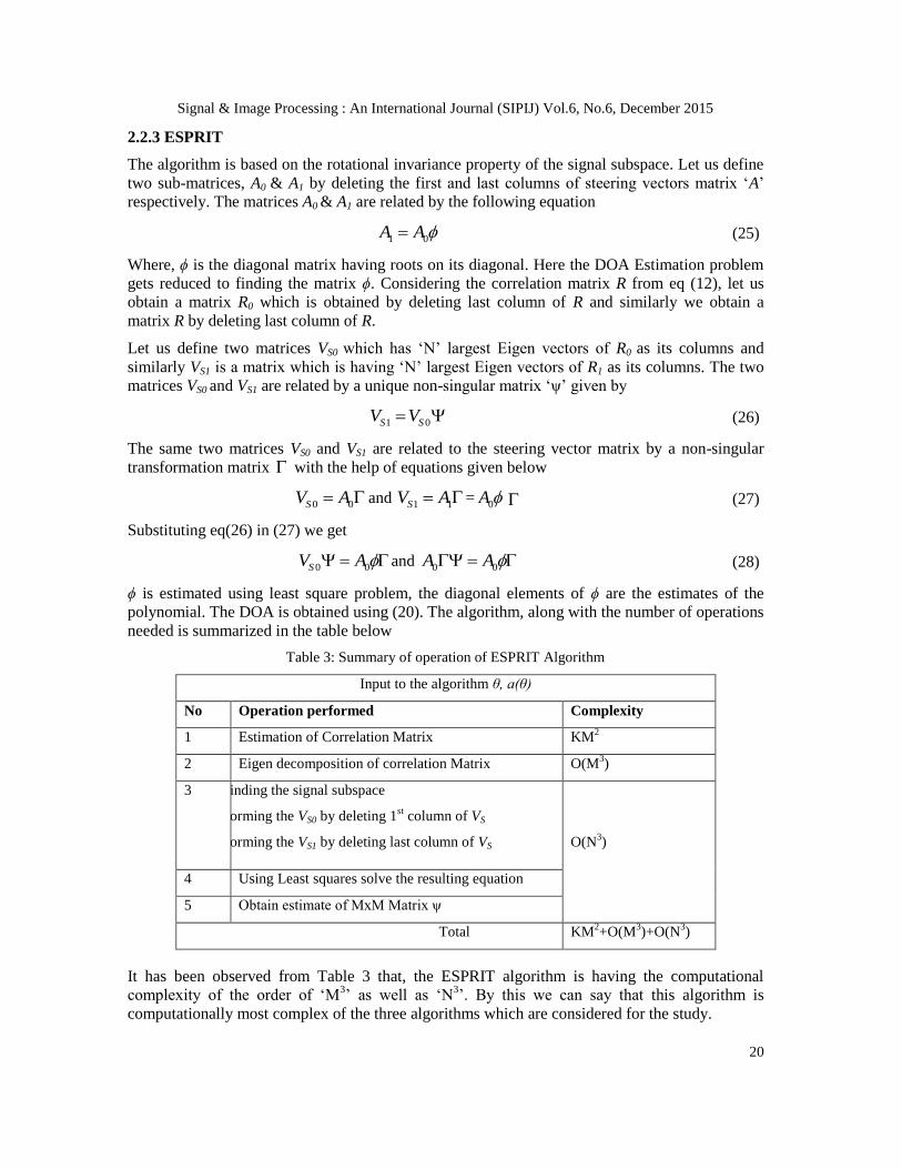
2.2.3 ESPRIT
The algorithm is based on the rotational invariance property of the signal subspace. Let us define
two sub-matrices, A0 & A1 by deleting the first and last columns of steering vectors matrix „A‟
respectively. The matrices A0 & A1 are related by the following equation
1 0A A (25)
Where, ϕ is the diagonal matrix having roots on its diagonal. Here the DOA Estimation problem
gets reduced to finding the matrix ϕ. Considering the correlation matrix R from eq (12), let us
obtain a matrix R0 which is obtained by deleting last column of R and similarly we obtain a
matrix R by deleting last column of R.
Let us define two matrices VS0 which has „N‟ largest Eigen vectors of R0 as its columns and
similarly VS1 is a matrix which is having „N‟ largest Eigen vectors of R1 as its columns. The two
matrices VS0 and VS1 are related by a unique non-singular matrix „ψ‟ given by
1 0S SV V (26)
The same two matrices VS0 and VS1 are related to the steering vector matrix by a non-singular
transformation matrix with the help of equations given below
0 0SV A and 1 1SV A = 0A (27)
Substituting eq(26) in (27) we get
0 0SV A and 0 0A A (28)
ϕ is estimated using least square problem, the diagonal elements of ϕ are the estimates of the
polynomial. The DOA is obtained using (20). The algorithm, along with the number of operations
needed is summarized in the table below
Table 3: Summary of operation of ESPRIT Algorithm
Input to the algorithm θ, a(θ)
No Operation performed Complexity
1 Estimation of Correlation Matrix KM2
2 Eigen decomposition of correlation Matrix O(M3)
3
Finding the signal subspace
Forming the VS0 by deleting 1st column of VS
Forming the VS1 by deleting last column of VS
O(N3)
4 Using Least squares solve the resulting equation
5 Obtain estimate of MxM Matrix ψ
Total KM2+O(M
3)+O(N
3)
It has been observed from Table 3 that, the ESPRIT algorithm is having the computational
complexity of the order of „M3‟ as well as „N
3‟. By this we can say that this algorithm is
computationally most complex of the three algorithms which are considered for the study.

Signal & Image Processing : An International Journal (SIPIJ) Vol.6, No.6, December 2015
21
2.3 Tracking the DOA The Kalman filter (KF) algorithm proposed by R.E.Kalman is considered as the basic of tracking
algorithms used in optimum filtering of non-stationary signals. KF algorithm also known as
dynamic filtering algorithm is considered as an advantage over the Weiner filter [2] [6] [16]
which fail to address the issue of non-stationarity. In DOA tracking we use KF filter to track the
optimum DOA estimate. The estimated DOA using one of the procedures above will act as an
initial estimate to the Kalman Filter algorithm. Based on the physical model, the algorithm starts
tracking the DOA Estimate. The KF algorithm is illustrated using the following steps.
2.3.1Tracking model
Let us consider θi(t), ( )i k , ( )i k ; i=1,2,3......q gives us the DOA, Angular velocity and angular
acceleration of the „q‟ number of sources at time T. The equations governing the motion of the ith
source are given by
1
2
3
( 1) ( ) ( )
( 1) ( ) ( )
( )( 1) ( )
i i i
i i i
i
k k k
k F k k
kk k
(29)
Where Matrix F is given by
2
12
0 1
0 0 1
TT
F T
(30)
Where T is the sampling duration and ωi(k), i=1,2,3....q are random process noise responsible for
the random disturbances. It is assumed that ωi(k) is zero mean white Gaussian noise with
covariances indicated as follows
[ ( ) ( )]T
i i iQ E k k (31)
In the tracking model illustrated above, we assume that the acceleration remains constant
throughout the sampling interval.
2.3.2 Tracking Algorithm
In the present study, single source is being tracked. The tracking algorithm is illustrated as
follows xi(k) is the state of the „q‟ sources at „k‟ and is given by

Signal & Image Processing : An International Journal (SIPIJ) Vol.6, No.6, December 2015
22
( )
( ) ( ) 1,2, ,
( )
i
i i
k
x k k i q
k
(32)
Using equation (29) the source motion governing model, we can write (30) as
( 1) ( ) ( )i i ix k Fx k k (33)
ˆ ( )i k is the optimum DOA Estimate of ( )i k based on the data obtained during the interval
[(kT,(k+1)T]. Based on this we can write the measurement equation as
ˆ ( ) ( ) ( ) 1,2,3, ,i i ik k k i q (34)
using equations (34) and considering the optimum DOA Estimate, a Kalman filter is used to track
the source‟s state estimate. The state estimation is carried out using the following components.
We can rewrite the equation (34) as
( )
ˆ ( ) ( ) ( ) 1,2,3, ,
( )
i
i i i
i
n
n h n n i q
n
(35)
Where h=[1,0,0] since we are going to track only angular position, we neglect the angular
velocities and acceleration and hence the „h‟ vector. Using Equations (32-35) the Kalman filter
equation can be written as
ˆ ( | 1)ˆ ( | )
ˆ ˆ ˆ( | ) ( | 1) ( )[ ( ) ( | 1)]
ˆ( | ) ( | 1)
ii
i i i i i
ii
n nn n
n n n n L n n n n
n n n n
(36)
The first term in the RHS of (36) are predicted estimates, the prediction is carried out using the
measurements up to (n-1) T.
The predicted state estimates of ˆ ( | )i n n , ( | )i n n , ( | )i n n are given by
ˆ ˆˆ[ ( | 1), ( | 1), ( | 1)]i i in n n n n n respectively. The Kalman gain Li(n) acts as a weighted
compensator is given by
1
( | 1)( )
( | 1)
T
ii T
ii
P n n hL n
hP n n h J
(37)
Where, Jii is the ith element of the Fisher information Matrix.
The Kalman filter recursions are carried out in the following steps
1. In the first interval, one of the optimum procedures to obtain DOA is used to find the
initial estimate of DOA.
Signal & Image Processing : An International Journal (SIPIJ) Vol.6, No.6, December 2015
23
2. In the next step we use the optimum DOA estimate as the initial value and start tracking
the DOA Estimates. The Kalman filter algorithm is summarised in Table 4
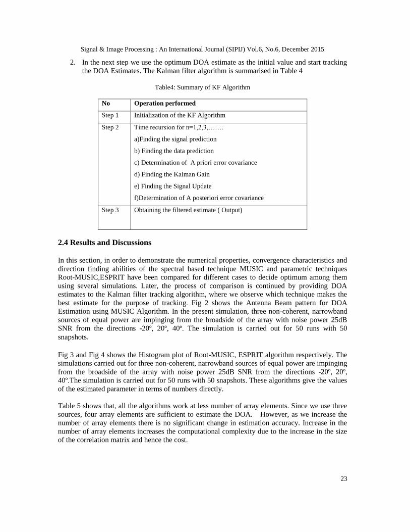
Table4: Summary of KF Algorithm
No Operation performed
Step 1 Initialization of the KF Algorithm
Step 2 Time recursion for n=1,2,3,…….
a)Finding the signal prediction
b) Finding the data prediction
c) Determination of A priori error covariance
d) Finding the Kalman Gain
e) Finding the Signal Update
f)Determination of A posteriori error covariance
Step 3
Obtaining the filtered estimate ( Output)
2.4 Results and Discussions In this section, in order to demonstrate the numerical properties, convergence characteristics and
direction finding abilities of the spectral based technique MUSIC and parametric techniques
Root-MUSIC,ESPRIT have been compared for different cases to decide optimum among them
using several simulations. Later, the process of comparison is continued by providing DOA
estimates to the Kalman filter tracking algorithm, where we observe which technique makes the
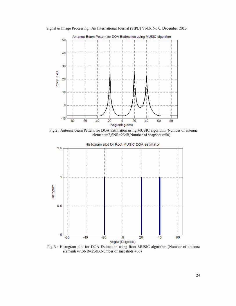
best estimate for the purpose of tracking. Fig 2 shows the Antenna Beam pattern for DOA
Estimation using MUSIC Algorithm. In the present simulation, three non-coherent, narrowband
sources of equal power are impinging from the broadside of the array with noise power 25dB
SNR from the directions -20º, 20º, 40º. The simulation is carried out for 50 runs with 50
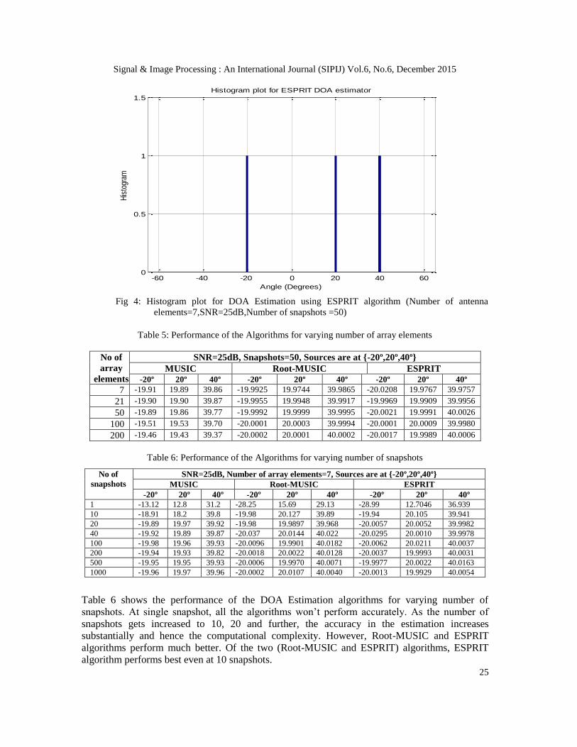
snapshots. Fig 3 and Fig 4 shows the Histogram plot of Root-MUSIC, ESPRIT algorithm respectively. The
simulations carried out for three non-coherent, narrowband sources of equal power are impinging
from the broadside of the array with noise power 25dB SNR from the directions -20º, 20º,
40º.The simulation is carried out for 50 runs with 50 snapshots. These algorithms give the values
of the estimated parameter in terms of numbers directly.
Table 5 shows that, all the algorithms work at less number of array elements. Since we use three
sources, four array elements are sufficient to estimate the DOA. However, as we increase the
number of array elements there is no significant change in estimation accuracy. Increase in the
number of array elements increases the computational complexity due to the increase in the size
of the correlation matrix and hence the cost.
Signal & Image Processing : An International Journal (SIPIJ) Vol.6, No.6, December 2015
24
Fig 2 : Antenna beam Pattern for DOA Estimation using MUSIC algorithm (Number of antenna
elements=7,SNR=25dB,Number of snapshots=50)
Fig 3 : Histogram plot for DOA Estimation using Root-MUSIC algorithm (Number of antenna
elements=7,SNR=25dB,Number of snapshots =50)
Signal & Image Processing : An International Journal (SIPIJ) Vol.6, No.6, December 2015
25
Fig 4: Histogram plot for DOA Estimation using ESPRIT algorithm (Number of antenna
elements=7,SNR=25dB,Number of snapshots =50)
Table 5: Performance of the Algorithms for varying number of array elements
No of
array
elements
SNR=25dB, Snapshots=50, Sources are at {-20º,20º,40º}
MUSIC Root-MUSIC ESPRIT
-20º 20º 40º -20º 20º 40º -20º 20º 40º
7 -19.91 19.89 39.86 -19.9925 19.9744 39.9865 -20.0208 19.9767 39.9757
21 -19.90 19.90 39.87 -19.9955 19.9948 39.9917 -19.9969 19.9909 39.9956
50 -19.89 19.86 39.77 -19.9992 19.9999 39.9995 -20.0021 19.9991 40.0026
100 -19.51 19.53 39.70 -20.0001 20.0003 39.9994 -20.0001 20.0009 39.9980
200 -19.46 19.43 39.37 -20.0002 20.0001 40.0002 -20.0017 19.9989 40.0006
Table 6: Performance of the Algorithms for varying number of snapshots
No of
snapshots
SNR=25dB, Number of array elements=7, Sources are at {-20º,20º,40º}
MUSIC Root-MUSIC ESPRIT
-20º 20º 40º -20º 20º 40º -20º 20º 40º
1 -13.12 12.8 31.2 -28.25 15.69 29.13 -28.99 12.7046 36.939
10 -18.91 18.2 39.8 -19.98 20.127 39.89 -19.94 20.105 39.941
20 -19.89 19.97 39.92 -19.98 19.9897 39.968 -20.0057 20.0052 39.9982
40 -19.92 19.89 39.87 -20.037 20.0144 40.022 -20.0295 20.0010 39.9978
100 -19.98 19.96 39.93 -20.0096 19.9901 40.0182 -20.0062 20.0211 40.0037
200 -19.94 19.93 39.82 -20.0018 20.0022 40.0128 -20.0037 19.9993 40.0031
500 -19.95 19.95 39.93 -20.0006 19.9970 40.0071 -19.9977 20.0022 40.0163
1000 -19.96 19.97 39.96 -20.0002 20.0107 40.0040 -20.0013 19.9929 40.0054
Table 6 shows the performance of the DOA Estimation algorithms for varying number of
snapshots. At single snapshot, all the algorithms won‟t perform accurately. As the number of
snapshots gets increased to 10, 20 and further, the accuracy in the estimation increases
substantially and hence the computational complexity. However, Root-MUSIC and ESPRIT
algorithms perform much better. Of the two (Root-MUSIC and ESPRIT) algorithms, ESPRIT
algorithm performs best even at 10 snapshots.
-60 -40 -20 0 20 40 600
0.5
1
1.5Histogram plot for ESPRIT DOA estimator
Angle (Degrees)
His
togr
am

Signal & Image Processing : An International Journal (SIPIJ) Vol.6, No.6, December 2015
26
Table 7: Performance of the Algorithms for varying SNR
SNR
(dB)
Number of snapshots=50, Number of array elements=7, Sources are at {-20º,20º,40º}
MUSIC Root-MUSIC ESPRIT
-20º 20º 40º -20º 20º 40º -20º 20º 40º
1 -19.12 21.2 38.3 -19.8053 19.8053 39.1318 -20.5167 19.9382 39.9006
2 -20.91 19.1 39.4 -19.2629 19.9044 39.6671 -19.3558 19.9956 39.7850
5 -20.43 19.13 40.25 -20.1338 19.2283 40.0051 -20.1967 19.1323 39.9528
10 -19.18 19.63 39.65 -19.9368 19.8121 39.9518 -19.9845 19.9206 39.9025
25 -19.89 19.88 40.23 -19.9976 19.9751 40.0148 -20.0001 19.9868 39.9958
50 -19.81 19.86 39.87 -19.9998 20.0001 39.9994 -20.0037 19.9988 40.0007
80 -19.91 19.97 39.93 -20.0001 20.0006 40.0002 -20.0000 20.0004 39.9999
90 -19.94 19.99 39.99 -20.000 20.0000 40.0000 -20.0000 20.0000 40.0000
Table 7 shows the performance of the DOA Estimation algorithms for varying SNR. At low
SNR, the accuracy of MUSIC algorithms is not good whereas the Root-MUSIC, ESPRIT
algorithms perform relatively well. As increase SNR, the accuracy in the estimation increases in
the case of MUSIC algorithm. However, Root-MUSIC and ESPRIT algorithms perform much
better even at low SNR. Of the two (Root-MUSIC, ESPRIT) algorithms, ESPRIT performs much
better.
Later, a single moving source is considered and its estimated DOA is taken as an initial value and
is provided to the Kalman filter for the purpose of tracking. Here, 10º initial value is assumed, the
estimated DOA by all the three algorithms is given to Kalman filter model for tracking and the
performance is analysed for each algorithm.
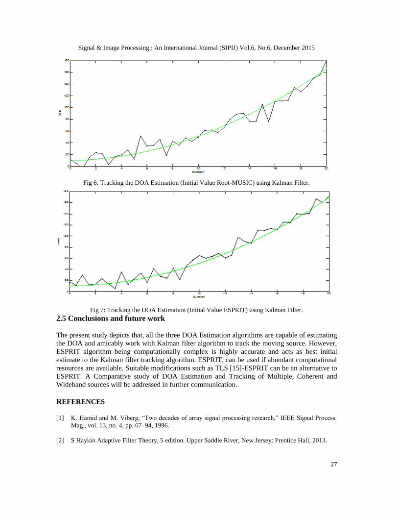
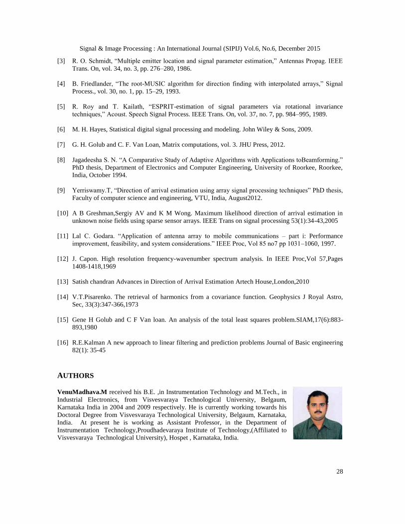
The Figs 5,6 and 7depict the performance of Kalman filter algorithm for the initial value
estimated using MUSIC, Root-MUSIC, and ESPRIT algorithms respectively. The KF tracking
algorithm is able to track the source whose initial value is estimated by all the DOA Estimation
algorithms from 10º to 170º. Of the three algorithms considered above, tracking the initial
estimate using ESPRIT algorithm is found to be better compared to other two techniques.
Fig 5: Tracking the DOA Estimation ( Initial Value MUSIC) using Kalman Filter.
Signal & Image Processing : An International Journal (SIPIJ) Vol.6, No.6, December 2015
27
Fig 6: Tracking the DOA Estimation (Initial Value Root-MUSIC) using Kalman Filter.
Fig 7: Tracking the DOA Estimation (Initial Value ESPRIT) using Kalman Filter.
2.5 Conclusions and future work
The present study depicts that, all the three DOA Estimation algorithms are capable of estimating
the DOA and amicably work with Kalman filter algorithm to track the moving source. However,
ESPRIT algorithm being computationally complex is highly accurate and acts as best initial
estimate to the Kalman filter tracking algorithm. ESPRIT, can be used if abundant computational
resources are available. Suitable modifications such as TLS [15]-ESPRIT can be an alternative to
ESPRIT. A Comparative study of DOA Estimation and Tracking of Multiple, Coherent and
Wideband sources will be addressed in further communication.
REFERENCES
[1] K. Hamid and M. Viberg, “Two decades of array signal processing research,” IEEE Signal Process.
Mag., vol. 13, no. 4, pp. 67–94, 1996.
[2] S Haykin Adaptive Filter Theory, 5 edition. Upper Saddle River, New Jersey: Prentice Hall, 2013.
Signal & Image Processing : An International Journal (SIPIJ) Vol.6, No.6, December 2015
28
[3] R. O. Schmidt, “Multiple emitter location and signal parameter estimation,” Antennas Propag. IEEE
Trans. On, vol. 34, no. 3, pp. 276–280, 1986.
[4] B. Friedlander, “The root-MUSIC algorithm for direction finding with interpolated arrays,” Signal
Process., vol. 30, no. 1, pp. 15–29, 1993.
[5] R. Roy and T. Kailath, “ESPRIT-estimation of signal parameters via rotational invariance
techniques,” Acoust. Speech Signal Process. IEEE Trans. On, vol. 37, no. 7, pp. 984–995, 1989.
[6] M. H. Hayes, Statistical digital signal processing and modeling. John Wiley & Sons, 2009.
[7] G. H. Golub and C. F. Van Loan, Matrix computations, vol. 3. JHU Press, 2012.
[8] Jagadeesha S. N. “A Comparative Study of Adaptive Algorithms with Applications toBeamforming.”
PhD thesis, Department of Electronics and Computer Engineering, University of Roorkee, Roorkee,
India, October 1994.
[9] Yerriswamy.T, “Direction of arrival estimation using array signal processing techniques” PhD thesis,
Faculty of computer science and engineering, VTU, India, August2012.
[10] A B Greshman,Sergiy AV and K M Wong. Maximum likelihood direction of arrival estimation in
unknown noise fields using sparse sensor arrays. IEEE Trans on signal processing 53(1):34-43,2005
[11] Lal C. Godara. “Application of antenna array to mobile communications – part i: Performance
improvement, feasibility, and system considerations.” IEEE Proc, Vol 85 no7 pp 1031–1060, 1997.
[12] J. Capon. High resolution frequency-wavenumber spectrum analysis. In IEEE Proc,Vol 57,Pages
1408-1418,1969
[13] Satish chandran Advances in Direction of Arrival Estimation Artech House,London,2010
[14] V.T.Pisarenko. The retrieval of harmonics from a covariance function. Geophysics J Royal Astro,
Sec, 33(3):347-366,1973
[15] Gene H Golub and C F Van loan. An analysis of the total least squares problem.SIAM,17(6):883-
893,1980
[16] R.E.Kalman A new approach to linear filtering and prediction problems Journal of Basic engineering
82(1): 35-45
AUTHORS
VenuMadhava.M received his B.E. ,in Instrumentation Technology and M.Tech., in
Industrial Electronics, from Visvesvaraya Technological University, Belgaum,
Karnataka India in 2004 and 2009 respectively. He is currently working towards his
Doctoral Degree from Visvesvaraya Technological University, Belgaum, Karnataka,
India. At present he is working as Assistant Professor, in the Department of
Instrumentation Technology,Proudhadevaraya Institute of Technology,(Affiliated to
Visvesvaraya Technological University), Hospet , Karnataka, India.
Signal & Image Processing : An International Journal (SIPIJ) Vol.6, No.6, December 2015
29
Dr. S. N. Jagadeesha received his B.E., in Electronics and Communication
Engineering, from University B. D. T College of Engineering., Davangere affiliated to
Mysore University, Karnataka, India in 1979, M..E. from Indian Institute of Science
(IISC), Bangalore, India specializing in Electrical Communication Engineering., in
1987 and Ph.D. in Electronics and Computer Engineering., from University of
Roorkee (I.I.T, Roorkee), Roorkee, India in 1996. He is an IEEE member and Fellow,
IETE. His research interest includes Array Signal Processing, Wireless Sensor
Networks and Mobile Communications. He has published and presented many papers
on Adaptive Array Signal Processing and Direction-of-Arrival estimation. Currently he is Professor in the
Department of Computer Science and Engineering, Jawaharlal Nehru National College of Engg. (Affiliated
to Visvesvaraya Technological University), Shimoga, Karnataka, India.
Dr.Yerriswamy received his B.E. in Electronics and Communication Engineering,
From RYMEC, Bellary affiliated to Gulbarga University, Gulbarga, Karnataka, India
in 2000,M.Tech in Network and Internet Engineering from JNNCE, Shimoga,
Affiliated to Visvesvaraya Technological University, Belgaum, India in 2005 and
Ph.D in the Faculty of Computer and Information Science form Visvesvaraya
Technological University , Belgaum, Karnataka, India He is a member of ISTE. His
research interests includes Array Signal Processing, Wireless Sensor Networks,
Cognitive Radios. He has published many papers in Direction-of-Arrival estimation
and Array signal processing. Currently he is Professor in the Department of Computer science and
Engineering, KLE Institute of Technology, (Affiliated to Visvesvaraya Technological University,
Belgaum), Hubli, Karnataka, India