A Comparative Analysis of the Czech Republic and Hungary
39
A Comparative Analysis of the Czech Republic and Hungary Using Small Continuous-Time Macroeconometric Models Emil Stavrev 19 Reihe Transformationsökonomie Transition Economics Series
Transcript of A Comparative Analysis of the Czech Republic and Hungary

A Comparative Analysis of the Czech Republic and
Hungary Using Small Continuous-Time
Macroeconometric Models
Emil Stavrev
19
Reihe Transformationsökonomie
Transition Economics Series
A Comparative Analysis of the Czech Republic and Hungary
Using Small Continuous-Time Macroeconometric Models
Emil Stavrev
July 2000
19
Reihe Transformationsökonomie
Transition Economics Series
Institut für Höhere Studien (IHS), Wien Institute for Advanced Studies, Vienna
Contact: Emil Stavrev Czech National Bank Economic Modelling Division Na Prikope 28 115 03 Prague 1, Czech Republic email: [email protected]
Founded in 1963 by two prominent Austrians living in exile – the sociologist Paul F. Lazarsfeld and the
economist Oskar Morgenstern – with the financial support from the Ford Foundation, the Austrian
Federal Ministry of Education and the City of Vienna, the Institute for Advanced Studies (IHS) is the
first institution for postgraduate education and research in economics and the social sciences in
Austria. The Transition Economics Series presents research done at the Department of Transition
Economics and aims to share “work in progress” in a timely way before formal publication. As usual,
authors bear full responsibility for the content of their contributions.
Das Institut für Höhere Studien (IHS) wurde im Jahr 1963 von zwei prominenten Exilösterreichern –
dem Soziologen Paul F. Lazarsfeld und dem Ökonomen Oskar Morgenstern – mit Hilfe der Ford-
Stiftung, des Österreichischen Bundesministeriums für Unterricht und der Stadt Wien gegründet und ist
somit die erste nachuniversitäre Lehr- und Forschungsstätte für die Sozial- und Wirtschafts-
wissenschaften in Österreich. Die Reihe Transformationsökonomie bietet Einblick in die
Forschungsarbeit der Abteilung für Transformationsökonomie und verfolgt das Ziel, abteilungsinterne
Diskussionsbeiträge einer breiteren fachinternen Öffentlichkeit zugänglich zu machen. Die inhaltliche
Verantwortung für die veröffentlichten Beiträge liegt bei den Autoren und Autorinnen.
Abstract
In this paper we estimate a continuous-time macroeconometric model of the Hungarian
economy and compare it with the Czech model described in Stavrev (1998). On the basis of
the estimated models we provide simulations and compare the results between the two
countries for i) anti-inflationary policy; ii) monetary and fiscal policies; iii) the effect of different
wage indexation schemes; iv) the effect of nominal wage rigidities and v) the effect of price
and nominal wage freeze.
Keywords Lucas critique, policy simulations, macroeconometric model, anti-inflationary policy, effectiveness
of monetary and fiscal policies
JEL Classifications C51, C52, C53, E17, E50, E52

Comments
This research was undertaken with support from the European Union’s Phare ACE Programme 1996.
I would like to thank Prof. S. Reynolds, Assistant Prof. E. Koèenda, Prof. R. Filer, Prof. J. Kmenta, Prof.
A. Wörgötter, and my colleagues at The Centre for Economic Research and Graduate Education, and
the Institute for Advanced Studies in Vienna for many helpful comments. All errors, however, are mine.
Contents
1. Introduction 1
2. Hungarian Model 2 2.1. Specification of the Equations............................................................................................. 2 2.2. Econometric Results ........................................................................................................... 8
3. Comparative Study of the Czech Republic and Hungary Based on the Model Simulations 10 3.1. Simulations with Macro-Econometric Models and Lucas Critique .................................... 10 3.2. Anti-inflationary Policies .....................................................................................................11
3.2.1. The Effect of Money Supply on Inflation................................................................. 12 3.2.2. The Effect of Wages on Inflation............................................................................. 13
3.3. Excluding Foreign Prices from Wage Indexation .............................................................. 13 3.4. The Impact of Wage Adjustment ....................................................................................... 14 3.5. The Impact of Price and Wage Freeze ............................................................................. 15 3.6. Effectiveness of Monetary and Fiscal Policies.................................................................. 15
4. Conclusions 16
References 17
Appendix 1. Data Description 20
Appendix 2. The Czech Model 23
Appendix 3. Effectiveness of Monetary and Fiscal Policies 24
Appendix 4. Anti-inflationary Policies 27 A4.1. The Effect of Money Supply on Inflation......................................................................... 27 A4.2. The Effect of Wages on Inflation..................................................................................... 28
Appendix 5. Excluding Foreign Prices from Wage Indexation 29
Appendix 6. The Impact of Wage Adjustment 30
Appendix 7. The Impact of Price and Wage Freeze 31
I H S — Stavrev / A Comparative Analysis of the Czech Republic and Hungary — 1
1. Introduction
The aim of this paper, on the basis of estimated macroeconometric models for the Czech
Republic and Hungary, is to compare different policy simulations for the two countries in
transitions. In particular we are interested in anti-inflationary policy, the mix of fiscal and
monetary policies and exchange rate policy.
We have chosen the Czech Republic and Hungary because of several similarities with
respect to their period of transition to a market economy. Both countries experienced a
period of initial fall of the real GDP in the early nineties and resumed real GDP growth in
1994. Some of the main macroeconomic indicators for the two economies are given in Table
1 below.
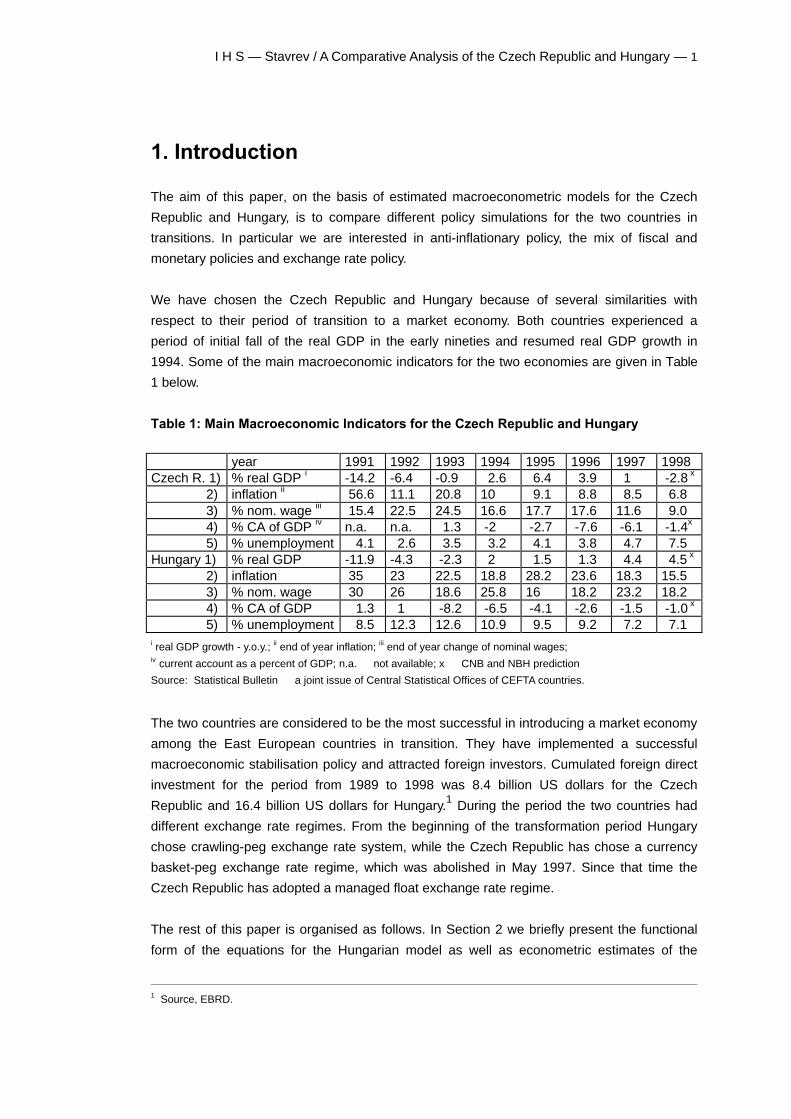
Table 1: Main Macroeconomic Indicators for the Czech Republic and Hungary
year 1991 1992 1993 1994 1995 1996 1997 1998 Czech R. 1) % real GDP i -14.2 -6.4 -0.9 2.6 6.4 3.9 1 -2.8 x 2) inflation ii 56.6 11.1 20.8 10 9.1 8.8 8.5 6.8 3) % nom. wage iii 15.4 22.5 24.5 16.6 17.7 17.6 11.6 9.0 4) % CA of GDP iv n.a. n.a. 1.3 -2 -2.7 -7.6 -6.1 -1.4x 5) % unemployment 4.1 2.6 3.5 3.2 4.1 3.8 4.7 7.5 Hungary 1) % real GDP -11.9 -4.3 -2.3 2 1.5 1.3 4.4 4.5 x 2) inflation 35 23 22.5 18.8 28.2 23.6 18.3 15.5 3) % nom. wage 30 26 18.6 25.8 16 18.2 23.2 18.2 4) % CA of GDP 1.3 1 -8.2 -6.5 -4.1 -2.6 -1.5 -1.0 x 5) % unemployment 8.5 12.3 12.6 10.9 9.5 9.2 7.2 7.1 i real GDP growth - y.o.y.; ii end of year inflation; iii end of year change of nominal wages; iv current account as a percent of GDP; n.a. not available; x CNB and NBH prediction
Source: Statistical Bulletin a joint issue of Central Statistical Offices of CEFTA countries.
The two countries are considered to be the most successful in introducing a market economy
among the East European countries in transition. They have implemented a successful
macroeconomic stabilisation policy and attracted foreign investors. Cumulated foreign direct
investment for the period from 1989 to 1998 was 8.4 billion US dollars for the Czech
Republic and 16.4 billion US dollars for Hungary.1 During the period the two countries had
different exchange rate regimes. From the beginning of the transformation period Hungary
chose crawling-peg exchange rate system, while the Czech Republic has chose a currency
basket-peg exchange rate regime, which was abolished in May 1997. Since that time the
Czech Republic has adopted a managed float exchange rate regime.
The rest of this paper is organised as follows. In Section 2 we briefly present the functional
form of the equations for the Hungarian model as well as econometric estimates of the
1 Source, EBRD.
2 — Stavrev / A Comparative Analysis of the Czech Republic and Hungary — I H S
parameters. In Section 3 we provide a comparative analysis between the two countries using
the estimated models from this paper and Stavrev (1998), while Section 4 concludes.
2. Hungarian Model
In this section we will briefly describe the structure of the Hungarian model. We construct the
model following closely the theoretical considerations explained in detail in Stavrev (1998).
For a complete discussion of the theoretical basis of continuous-time macro models see
Bergstrom (1990), Gandolfo (1981, 1993) and Gandolfo and Padoan (1984). It should be
mentioned that both the Czech and Hungarian models are very similar in construction. We
exploit this similarity in order to be able to compare the results about the two countries when
using the models later in the simulation exercises.
2.1. Specification of the Equations
The model is an interdependent system of stochastic differential equations. To simplify, the
disturbance terms are omitted. The symbol (^) refers to the partial equilibrium level, or the
desired value of the variable, (e) to its expectation, and ln to the natural logarithm. All
parameters are assumed to be positive unless otherwise specified.
Consumption function
DlnC = α1ln$C
C
+ α2 m2 (1)
where
$C = γ1 Y where γ1 is marginal propensity to consume (1.1)
C − real consumption2
m2 − proportional rate of change of money supply (M2)
Y − real gross domestic product
In equation (1) real aggregate consumption,3 C, adjusts to its desired level, $C , which is
given as the marginal propensity to consume applied to real domestic income. The second
2 For a detailed specification of the data see Appendix 1.
I H S — Stavrev / A Comparative Analysis of the Czech Republic and Hungary — 3
term in this equation must capture the impact of the monetary variables, proxied by m2, on
consumption. The idea is that nominal money balances play a buffer role in the private sector
asset portfolio, allowing unexpected variations in income and expenditure.
Imports
DlnIm = α3 ln$ImIm
+ α4 ln
$VV
(2)
where
I $m = γ2 P
P Qf
β1
(DK) β2 Cβ3 Eβ4 (2.1)
$V = γ4Y e, (2.2)
Im − real imports
V − stock of inventories in real terms
DK − change of fixed capital stock in real terms
Pf − foreign price level4
P − domestic price level (CPI)
E − real exports
Q − nominal exchange rate
3 Precisely speaking, in equation (1) and in the following equations we define the rate of change in the left hand side variables as opposed to their real levels, but after the integration of the system (1) − (12) we will obtain the levels of the variables. 4 For the estimation we use the price level in the rest of the world, which is constructed as a weighted average of US and German price levels as follows: Pf =w*eDM$* Pus + (1-w)*PGer where w is the weight of the US dollar taken according to the definition given in Appendix 1 and eDM$ is the exchange rate of the US dollar with respect to the German mark. Thus, the price index for the rest of the world is expressed in German marks. We obtain income for the rest of the world in the same way.
4 — Stavrev / A Comparative Analysis of the Czech Republic and Hungary — I H S
Real imports defined in equation (2) are determined by two terms. First, they adjust to their
desired value $Im , which is a function of real exchange rate and consumption and
investment expenditures. This specification connects demand for imports to total sales and
takes into account the fact that some imported goods are included in exports. Second,
imports are connected to the change in inventories. If inventories are less than their desired
level, imports will increase. Hence, inventories are supposed to play a buffer role between
supply and demand in the goods market.
Exports
DlnE = α5 ln$EE
(3)
where
$E = γβ
β3
5
6P
P QY
ff
−
(3.1)
Yf − real foreign income
Equation (3) defines the demand for real exports of goods and services. Their partial
equilibrium level depends on real exchange rate and foreign income. The export equation in
the Hungarian model differs from the one used in the Czech model. Taking into account the
differences in the exchange rate systems Hungary has a crawling-peg system and the
Czech Republic for most of the sample period had a fixed exchange rate we have decided
to relate Hungarian exports to real exchange rate and foreign income.
Expected output
DlnY e = ξ lnY
Y e
(4)
Y e − expected output
Equation (4) defines expected output. Expected output evolves according to an adaptive
expectation mechanism and has two functions in the model. In addition to determining real
output, it connects real output to the rest of the model by the presence of the second term in
equation (5) below.
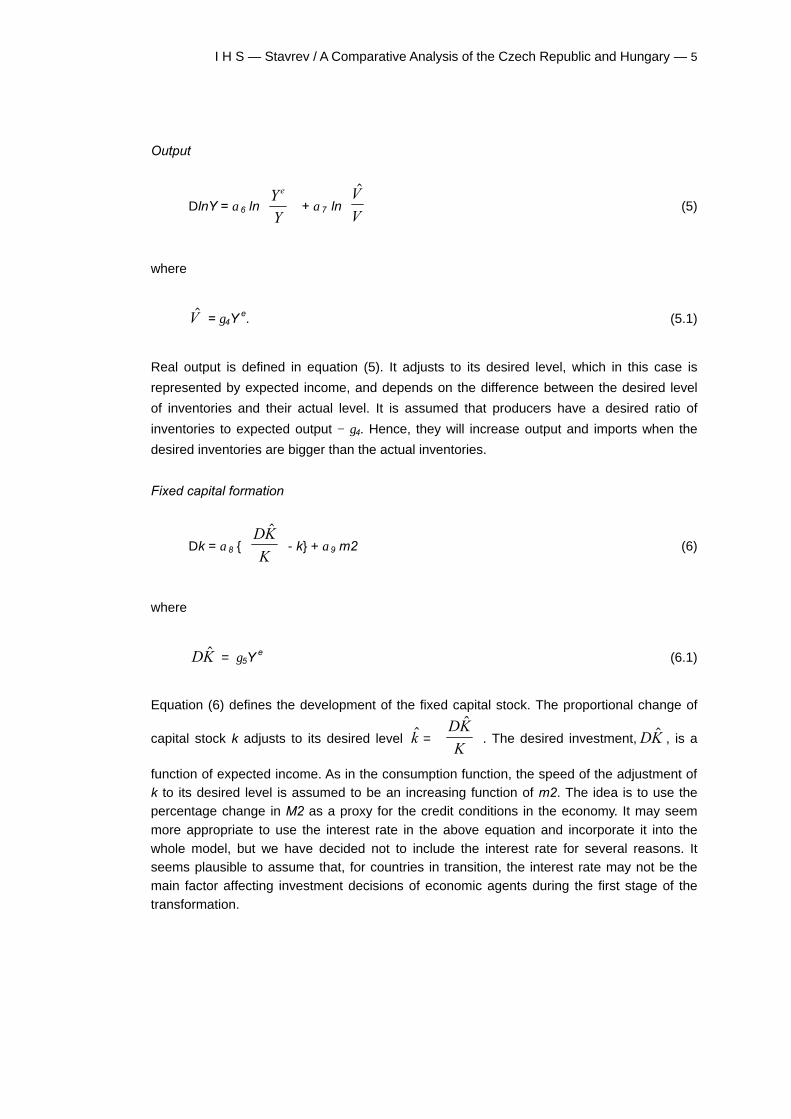
I H S — Stavrev / A Comparative Analysis of the Czech Republic and Hungary — 5
Output
DlnY = α6 lnYY
e
+ α7 ln
$VV
(5)
where
$V = γ4Y e. (5.1)
Real output is defined in equation (5). It adjusts to its desired level, which in this case is
represented by expected income, and depends on the difference between the desired level
of inventories and their actual level. It is assumed that producers have a desired ratio of
inventories to expected output − γ4. Hence, they will increase output and imports when the
desired inventories are bigger than the actual inventories.
Fixed capital formation
Dk = α8 {DKK
$
- k} + α9 m2 (6)
where
DK$ = γ5Y e (6.1)
Equation (6) defines the development of the fixed capital stock. The proportional change of
capital stock k adjusts to its desired level $k = DKK
$
. The desired investment, DK$ , is a
function of expected income. As in the consumption function, the speed of the adjustment of k to its desired level is assumed to be an increasing function of m2. The idea is to use the percentage change in M2 as a proxy for the credit conditions in the economy. It may seem
more appropriate to use the interest rate in the above equation and incorporate it into the
whole model, but we have decided not to include the interest rate for several reasons. It seems plausible to assume that, for countries in transition, the interest rate may not be the
main factor affecting investment decisions of economic agents during the first stage of the
transformation.
6 — Stavrev / A Comparative Analysis of the Czech Republic and Hungary — I H S
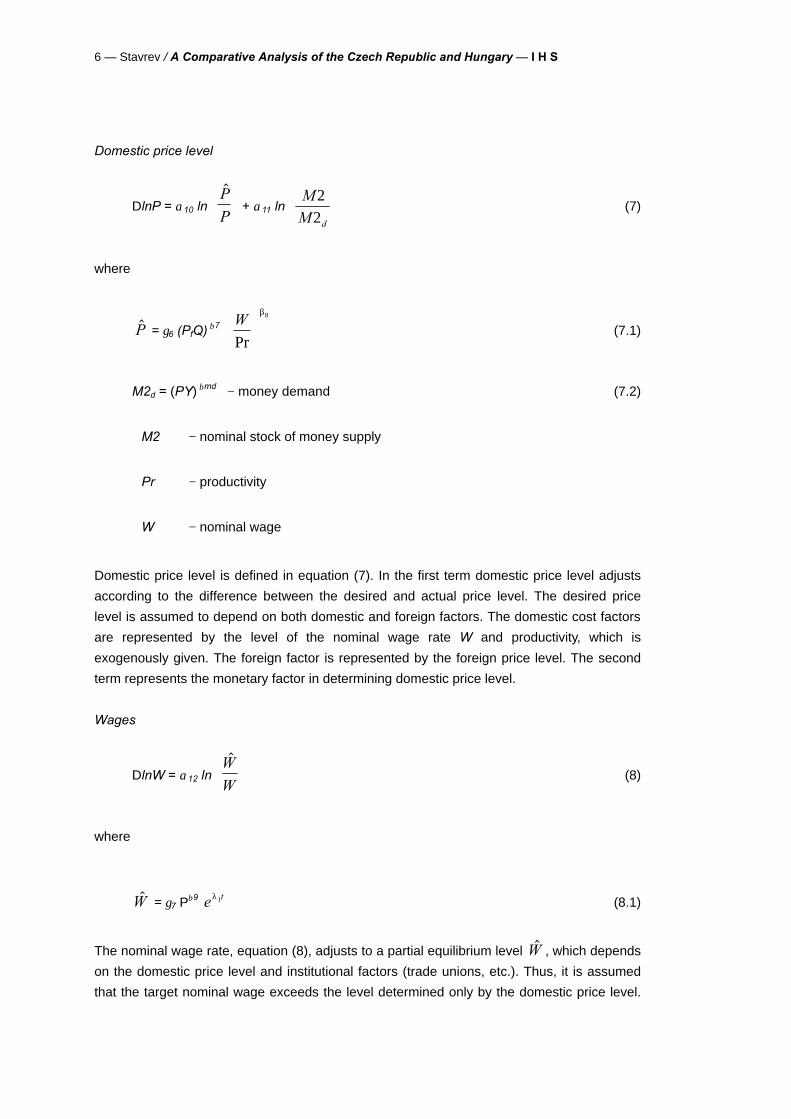
Domestic price level
DlnP = α10 ln$PP
+ α11 ln
MM d
22
(7)
where
$P = γ6 (PfQ) β7
WPr
β8
(7.1)
M2d = (PY) βmd − money demand (7.2)
M2 − nominal stock of money supply
Pr − productivity
W − nominal wage
Domestic price level is defined in equation (7). In the first term domestic price level adjusts
according to the difference between the desired and actual price level. The desired price
level is assumed to depend on both domestic and foreign factors. The domestic cost factors
are represented by the level of the nominal wage rate W and productivity, which is
exogenously given. The foreign factor is represented by the foreign price level. The second
term represents the monetary factor in determining domestic price level.
Wages
DlnW = α12 ln$W
W
(8)
where
$W = γ7 Pβ9 e tλ1 (8.1)
The nominal wage rate, equation (8), adjusts to a partial equilibrium level $W , which depends
on the domestic price level and institutional factors (trade unions, etc.). Thus, it is assumed
that the target nominal wage exceeds the level determined only by the domestic price level.
I H S — Stavrev / A Comparative Analysis of the Czech Republic and Hungary — 7
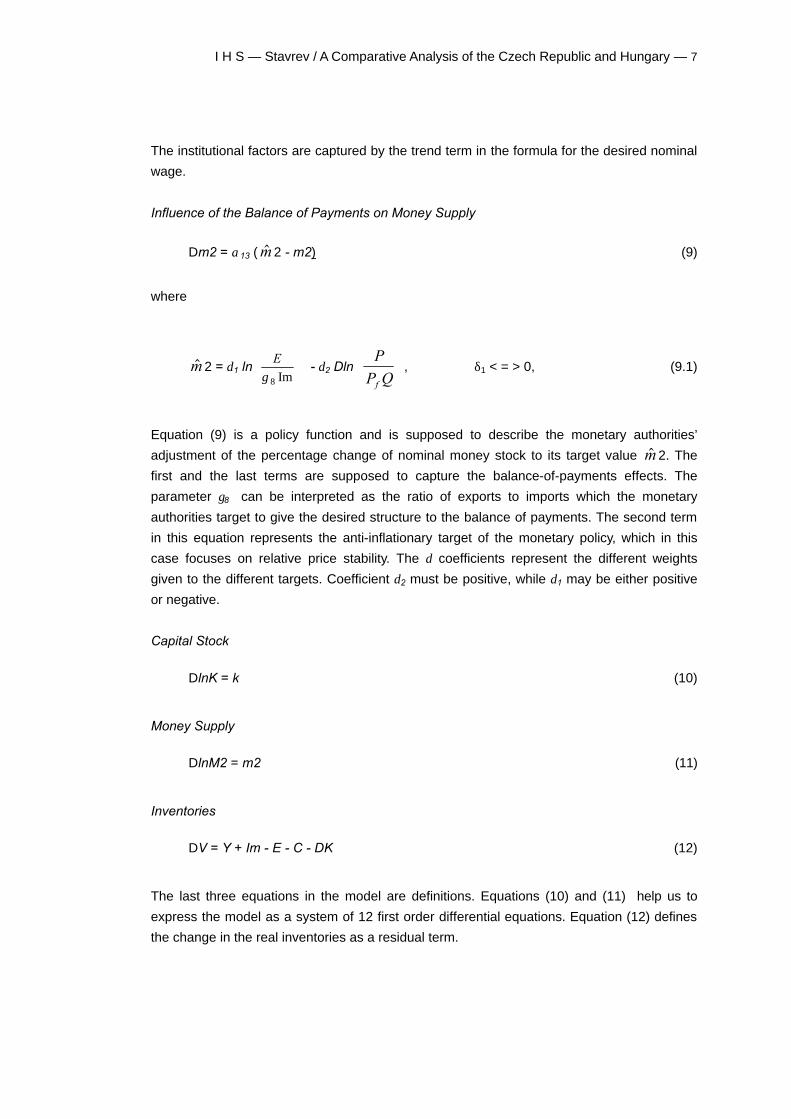
The institutional factors are captured by the trend term in the formula for the desired nominal
wage.
Influence of the Balance of Payments on Money Supply
Dm2 = α13 ( $m 2 - m2) (9)
where
$m 2 = δ1 lnE
γ 8 Im
- δ2 Dln
PP Qf
, δ1 < = > 0, (9.1)
Equation (9) is a policy function and is supposed to describe the monetary authorities’
adjustment of the percentage change of nominal money stock to its target value $m 2. The
first and the last terms are supposed to capture the balance-of-payments effects. The
parameter γ8 can be interpreted as the ratio of exports to imports which the monetary
authorities target to give the desired structure to the balance of payments. The second term
in this equation represents the anti-inflationary target of the monetary policy, which in this
case focuses on relative price stability. The δ coefficients represent the different weights
given to the different targets. Coefficient δ2 must be positive, while δ1 may be either positive
or negative.
Capital Stock
DlnK = k (10)
Money Supply
DlnM2 = m2 (11)
Inventories
DV = Y + Im - E - C - DK (12)
The last three equations in the model are definitions. Equations (10) and (11) help us to
express the model as a system of 12 first order differential equations. Equation (12) defines
the change in the real inventories as a residual term.
8 — Stavrev / A Comparative Analysis of the Czech Republic and Hungary — I H S
There are 12 equations and 12 endogenous variables in the model. The only exogenous
variables in the model are time − t, productivity − Pr, foreign price level − Pf and foreign
income − Yf.
2.2. Econometric Results
We present the estimated equations for the Hungarian model below.5 Standard errors are
given in brackets. For simplicity the error terms are omitted.
DlnC = 0 390 14.( . )
ln0 75. Y
C
+ 3360 75.
( . )m2 (1’)
DlnIm = 0 790 16.
( . )ln
178 5550 5
1 930 17 0 32 0 250 85
0 07 0 23.
Im
( . )
.. . .( . )
( . ) ( . )P
P QDK C E
f
+ 0 020 08.
( . )ln
105. Y
V
e
(2’)
DlnE = 0 360 1.
( . )ln
2 410 45
2 2210 74
.( . )
..P
P QY
E
ff
(3’)
DlnY = 0 750 12.
( . )ln
YY
e
+ 0 02
0 004.
( . ) ln
105. Y
V
e
(5’)
Dk = 0850 14.
( . )
0140 04.
( . )Y
Kk
e
−
+ 0 25
0 04.
( . )m2 (6’)
DlnP = 0 430 15).
( .ln
0 020 01
1 390 36
00
. ( )Pr( . )
..
( .15)( .14)
P QW
P
f
+ 0 070 07.
( . )ln
M
PY
21( )
(7’)
5 Full description of the Czech model is given in Stavrev (1998). In Appendix 2 of this paper we present only the estimated equations of the model.
I H S — Stavrev / A Comparative Analysis of the Czech Republic and Hungary — 9
DlnW = 1140 22.
( . )ln
28454 51112 5)
0 14 0 040 04 0 0048.
( .
. .( . ) ( . )P e
W
t
(8’)
Dm2 = 1170 15.
( . ) { 0 02
0 003.
( . )ln
E0 880 413. Im
( . )
- 0 77
0 26.
( . )Dln
PP Qf
- m2}, (9’)
In this model we have estimated 13 adjustment speeds and buffer stock effects (the α -
parameters). Only two of them, the buffer stock coefficient α4 capturing the effect of
inventories on real imports in equation (2) and α11 reflecting the effect of money supply on
the price level in equation (11), are not significant at 5% level of significance. In addition to
the adjustment speed parameters we have 21 other parameters: constants, elasticities,
policy parameters and a trend term (γ, β, δ and λ correspondingly). Only one of them, β8
capturing the effect of productivity on price level, is not significant at 5% significance level.
We have estimated 34 parameters and only 3 of them are not significant at 5% level of
significance.
We will discuss several important factors in the estimation of some of the equations in the
Hungarian model. For the period from the first quarter of 1991 to the fourth quarter of 1995
there are no quarterly data on consumption and GDP for the Hungarian economy. There are,
however, quarterly data for exports, imports and fixed capital. In order to estimate equations
(1), (2) and (5) we construct for the period from first quarter of 1991 to fourth quarter of 1995
quarterly data for consumption and GDP according to the explanations given in Appendix 1.
Then we obtain the change in inventories as a residual term. In addition to this equations (1)
and (5) are estimated using the same structure of the equations as in the quarterly model
with annual data for the period from 1988 till 1997.
We conducted stability and sensitivity analyses exactly as in the Czech model. It should be
mentioned that all real parts of the characteristic roots of the parameter matrix are negative,
which indicates that the Hungarian model is locally stable.6
6 For extended stability and sensitivity analysis of the Czech macro model see Stavrev (1998).
10 — Stavrev / A Comparative Analysis of the Czech Republic and Hungary — I H S
3. Comparative Study of the Czech Republic and Hungary Based on the Model Simulations
The results of the simulations present in this section are given as deviations from the base
solution. We consider the effect of the different simulations on the following variables:
inflation rate DlnP, rate of growth of real consumption DlnC, rate of growth of fixed capital
DlnK, rate of growth of output DlnY, rate of growth of real wage rate Dln(W/P), and the
balance of goods and services TB, the last term defined as the ratio of the value of exports
to the value of imports Dln(E/Im). We will speak about improvement in inflation when DlnP
decreases, but improvement in output for example is connected with an increase in DlnY.
The same is true for the remaining variables.
3.1. Simulations with Macro-Econometric Models and Lucas Critique
Before explaining the simulations’ results we will discuss Lucas critique (Lucas, [1976]) and
its implications for the exercises we are using in this paper to evaluate alternative policies. In
what follows we will briefly present some of the most relevant arguments which have been
presented in the literature in defence of simulation analysis. It is by no means an attempt to
reject Lucas point, but rather to show that in some cases it is possible to use simulation
exercises for different policy evaluations.7 Moreover this method is even less vulnerable to
Lucas critique when one tests the properties of a macro-econometric model.
According to Gandolfo and Padoan (1984) simulation exercises may be classified four
different types: Type 1 exogenous variables are assumed to follow a different path from
the actual one; Type 2 endogenous variables, other than policy variables, are chosen to
follow a given time path; Type 3 there are policy changes which are uncertain and
insincere, meaning that policy makers either do not specify their present and future
behaviour or the policy they announce might be different from the one actually implemented;
Type 4 the policy change is sincere and once and for all, implying that the economic
agents have time to adjust their behaviour to the new policy regime.
Sims (1982) has pointed out that Lucas critique fully applies only to simulations of the fourth
type because economic agents have enough time and information to adjust their behaviour
to the new policy regime. Such events rarely happen in the real world and as an example we
may give the end of the Bretton-Wood system of exchange rates or the fixed exchange rate
system for the Czech Republic. Sims’ argument that “permanent shifts in policy regime are
by definition rare events” does not overcome the difficulty of dealing with a Type 4 policy
change.
7 For a more detailed discussion on the matter see Sims (1982) and Klein (1983).
I H S — Stavrev / A Comparative Analysis of the Czech Republic and Hungary — 11
Another argument, which seems more effective in solving this problem, is one suggested by
Jonson and Trevor (1981) that in the real world neither the policy maker nor the economic
agents really know how the system as a whole will react to the implementation of a new
policy rule. Consequently, it is a useful exercise, provided in-sample simulations are carried
out, to “rerun the history”, in order to obtain additional information on the behaviour of the
system (in the spirit of Vines, Miciejowsky and Meade[1983]).
If the policy makers do not specify in detail their planned strategy, the economic agents will
have difficulties trying to adjust their behaviour. It appears that Lucas critique is not
applicable when Type 3 policy rules are simulated. Moreover, policy makers quite often do
not have a completely clear idea of what their policy should be and, therefore, they will try to
define it by a trial-and-error process. It is clear then that uncertainty and insincerity might
arise not only as an explicit choice of the policy makers but from the fact that they need time
to work out their own way of applying the policy. Consequently, even if economic agents
have enough time to adjust to a given policy, this will change simply because the policy
makers will react to the system’s response.
With respect to Type 1 simulations, Mishkin (1979) argues that shocked values of exogenous
variables should be consistent with the time series model of historical values if simulation
results are reliable. This argument applies also when Type 2 simulations are carried out.
3.2. Anti-inflationary Policies
We believe that this type of policy simulations is of special importance for countries in
transition. After abandoning the system of command price-setting, all countries from the
formerly centrally planned economies experienced an initial period of high inflation.
Countries like the Czech Republic and Hungary managed to stop the inflation spiral and
achieved during the last four years an inflation of about 8.5 to 10% in the case of the Czech
Republic and 18 to 22% in the case of Hungary.
There are different hypotheses among economists about the causes of inflation in the
transition countries. Some economists argue that inflation was fuelled by the usually large
initial devaluation in the currencies of these countries. Other economists support the view
that price distortion (completely wrong relative prices inherited from the past) is the driving
force of inflation. We believe that in addition to the above reasons money supply and wages
may be to a great extent responsible for the relatively high inflation in the transition countries.
With the models we have built for the Czech Republic and Hungary we can simulate the
effect on inflation only of money supply and wages.
12 — Stavrev / A Comparative Analysis of the Czech Republic and Hungary — I H S
3.2.1. The Effect of Money Supply on Inflation
In order to study the effect of money supply on inflation we have used the following scheme.
The estimated equation about the monetary authorities’ reaction function in the two models
was replaced by the following one:
Dm m mt2 2 213= −α ( )* (13)
where m2*t is the “target growth” of M2 prescribed by the policy makers. For the simulation
exercises we assume that money supply grows in all four quarters of a particular year with
the same speed. The values of the growth of the money supply for the four quarters of a
particular year are chosen in such a way as to ensure a given yearly growth rate of the
money supply. The simulation period is from the first quarter of 1994 to the fourth quarter of
1997. The actual yearly growth rates of money supply for the simulation period are m A tCR2 , =
{20.9, 18.8, 9.2, 10.1} and m A tH2 , = {13.6, 18.4, 21.2, 22.9} for the Czech Republic and
Hungary respectively.8 For our simulations we have chosen quarterly growth rates of the
money supply of the two countries so as to achieve for the simulation period a cumulative
growth rate of money supply which is 5 percentage points lower than the cumulative growth
rate in the basic solution for both countries.
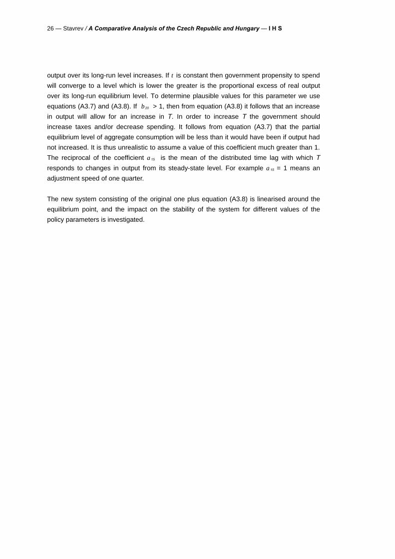
The results of these simulations are given in Appendix 4. The simulations given there are
produced using the Hungarian model. The results in the 12 figures in Appendix 4 represent
the difference between the target and basic solution. The impact of this policy simulation is
given on Figures A4.1 to A4.6. From Figure A4.1 we see that a 5% decrease in the growth
rate of money supply has decreased the inflation rate by 0.5%. Lowering the rate of growth
of money supply has a relatively strong impact on the real variables. Rate of growth of real
consumption to the end of the simulation period falls by 0.18%. It is easy to understand this
fact if we look at equation (1’). The effect on money supply is captured by the second term
and the coefficient there is quite high. As is mentioned above, the role of this term is to
capture the influence of wealth on consumption. There was a large privatisation in transition
countries which could be considered one of the sources of wealth increase. It is then
possible that consumers used this in order to increase their consumption. Capital stock is the
least affected among the real variables. The purpose of second term in capital formation
equation (6’) is to capture the effect of the credit conditions on investment. It may be the
case that market agents in transition countries will continue their investment plans even
under tougher investment conditions. One explanation is that they a expect higher return on
new productive capital because of the existence of a highly qualified and relatively cheap
work force. Real wages grow, but at a decreasing speed. The effect of this policy on the
trade balance is positive and at the end of the simulation period the current account gap is
decreased by 0.30%.
8 The data are in percents.
I H S — Stavrev / A Comparative Analysis of the Czech Republic and Hungary — 13
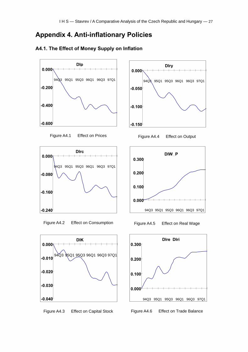
3.2.2. The Effect of Wages on Inflation
In order to evaluate the effect of wages on the economy we replace the equation for nominal
wages in the Hungarian the Czech model with the following one:
D W tln = λ , (14)
where t, stays for quarters. We have assumed that through out the simulation exercise the
rate of growth of nominal wages will be kept constant for each particular year. The actual
growth rates of the average nominal wages for the simulation period in the Czech Republic
and Hungary are λ A tCR
, = {17.8, 19.1, 16.8, 8} and λ A tH
, = {22.5, 15.2, 17.5, 24}
correspondingly. To study the effect of a wage decrease on inflation we have chosen λt so as
to obtain cumulative growth rate of wages 5% below the one of the basic solution for both
countries.
The impact of this policy simulation on macroeconomic variables is present in Appendix 4
Figures A4.7 to A4.12. Lower growth of wages decreases inflation. Since nominal wage
decreases slower than the price level (see the value of the coefficient β8 ) real wage growths.
At the beginning of the simulation period all real variables grow at a progressively declining
speed, and later decrease. As in the previous case the effect on capital stock is smaller.
Trade balance experiences a short period of improvement and after that a continuous
deterioration.
Under both anti-inflationary policy scenarios we have obtained the goal of lower inflation.
Money supply and wages have a comparable (in magnitude) effect on inflation
developments. The effect of money supply on the real variables, however, is stronger than
the effect of nominal wages.
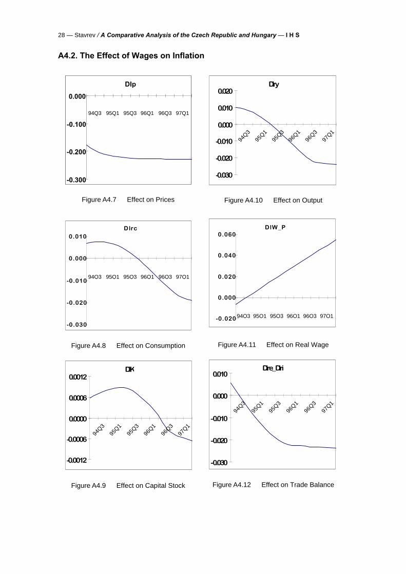
3.3. Excluding Foreign Prices from Wage Indexation
In this simulation we exclude imported inflation from the wage indexation mechanism
captured in nominal wage equations for the Czech and Hungarian models correspondingly.
In the new version of the wage equations we link nominal wages to the following price index,
which is corrected for foreign inflation:
PP
Pc
f
=β 6
. (15)

14 — Stavrev / A Comparative Analysis of the Czech Republic and Hungary — I H S
The impact of this policy simulation on the macroeconomic variables is described in
Appendix 5 Figures A5.1 to A5.6.9 Lower wage indexation results in lower than baseline
inflation. It improves on average by 0.25% per quarter. Inflation is lower through the whole
simulation period, though the major effect is in the first two years and then we observe
converging to the base line solution. A lower inflation rate under this scenario is obtained at
the cost of a lower real wage, which after two years starts returning to the control solution.
The average lost in real wage is around 0.12% per quarter. As a result of this, however, we
note a slight positive impact on real output and capital formation, especially during the first
two years. This increase in real output is export led. As a result of lower inflation we can
notice an improvement in competitiveness and thus an increase in real exports, which in turn
leads to improvement in real output at the beginning of the period. We obtain initial strong
improvement in balance of goods and services, which towards the end of the simulation
period deteriorates. The impact on real consumption is very low and it remains stable
through the simulation period. We record two different effects on consumption (consumption
depends on output and money supply growth; see equations for real consumption for both
models: on one side positive effect of output and on the other side negative effect of money
supply growth, which is lower than the baseline in this simulation.
3.4. The Impact of Wage Adjustment
In this policy simulation we study the impact of the speed of adjustment of wages on the
main macroeconomic variables specified at the beginning of Section 3. In order to do so we
replace the estimated speed of adjustment coefficient in the models, α12, which is around
one quarter for both economies with speed of adjustment of one year. The results of the
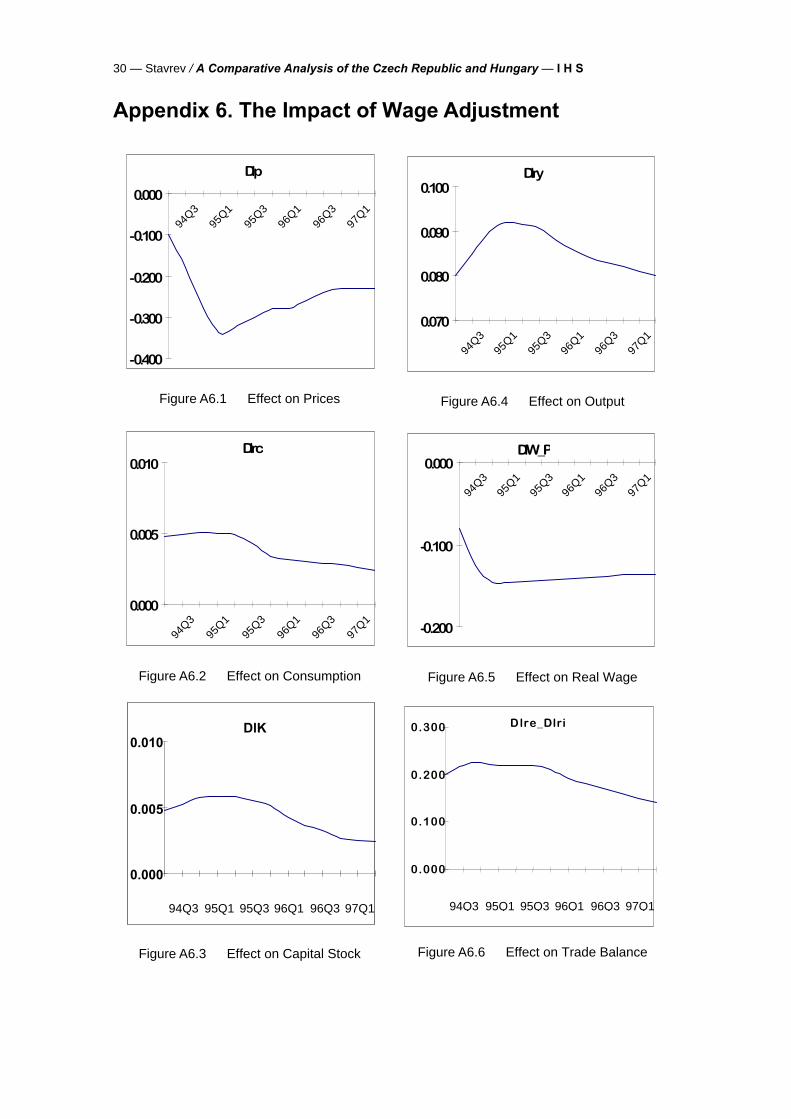
simulations with the Czech model are given in Appendix 6 Figures A6.1 to A6.6.
As in the previous case we note an improvement in inflation performance at the beginning of
the simulation period and deterioration in the real wage rate. Cumulative gain in inflation at
the end of the first year is around 1% and cumulative loss in real wages is around 0.6%. The
loss in real wages in this exercise is determined by the low adjustment of nominal wages
towards its target value. In the previous exercise the reason for the lower real wage was the
lower target of nominal wages, which did not account for the impact of foreign prices on
domestic inflation and thus wages were indexed at a lower speed. The effect on real output,
however, comes through the same transmission mechanism. Lower inflation supports higher
growth of real output through higher real exports. Improvement in the balance of goods and
services is greater at the beginning of the period and later on deteriorates as a result of the
consequent increase in inflation and relative loss of competitiveness.
9 In these simulations we use the Czech model. The response of the macro variables obtained from the Hungarian model is similar.
I H S — Stavrev / A Comparative Analysis of the Czech Republic and Hungary — 15
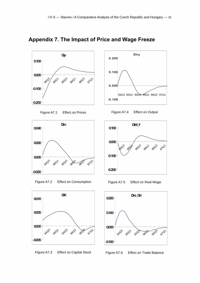
3.5. The Impact of Price and Wage Freeze
In this exercise we study the effect of both price and nominal wage rigidities on the
behaviour of the main macroeconomic variables. The results for the Czech model are given
in Appendix 7.
In this exercise we have three stages. During the first stage, which includes the first two
quarters of the simulation period, we set to zero the rate of growth of both prices and
nominal wages. During the second stage, which includes the next two quarters, domestic
prices rise at the same speed as foreign prices, but nominal wages are kept constant. During
the third stage the model is set back to its estimated structure. This exercise is useful since it
could induce some economic insights about the evolution of the main macroeconomic
variables following a sequence of price and wage freezes in the transition economies
resulting from price deregulation and wage bargaining with trade unions.
Under this policy we obtain a substantial decrease in inflation during the first year, but at the
beginning of the second year inflation is already higher than the control solution, remaining
on average 0.05% higher than the baseline scenario until the end of the period. At the
beginning of the period we note lower real wages than the baseline, followed by higher real
wages almost until the end of the simulations. The explanation about the existence of higher
real wages under this policy is that for most of the simulation interval (except for the first
year) wage formation is unchanged. This means that during the first two stages the
discrepancy between the actual and the desired level of the nominal wages rises
considerably. Then in the third phase, when the original mechanism operates, the growth
rate of nominal wages exceeds the growth rate of prices in the quarters immediately
following the end of the second stage, causing nominal wages to overshoot the baseline
solution. This fact, in turn, leads to acceleration of the wage-price spiral and as a result we
obtain higher inflation. Substantial improvement in competitiveness at the beginning leads to
higher exports and thus higher output for the first one and a half years. Inflation deterioration
later on has a negative impact on exports and through them on output as well.
3.6. Effectiveness of Monetary and Fiscal Policies
The effect of monetary and fiscal policies is studied using the framework described in
Appendix 3 below. We investigate the stability of both models under the two scenarios
presented there. Our criterion about the stability of the models is the sign of the real part of
the characteristic roots. A positive real part indicates an explosive solution. However, the
magnitude of the positive real part is important as well since relatively small positive values,
even though showing instability, allow us to use the model for policy simulations.
We calculate the characteristic roots for each of the two models under the two scenarios and
compare them with the values obtained solving the initial system of equations without the
16 — Stavrev / A Comparative Analysis of the Czech Republic and Hungary — I H S
introduction of fiscal policy rules. Both scenarios described in Appendix 3 have a stabilising
effect. In the case of the Czech Republic for “low taxation” policy in Scenario 1 we obtain a
system with no positive real part of the characteristic roots. As is mentioned in Section 2 of
this chapter the Hungarian model is locally stable. The introduction of both fiscal policy
scenarios makes the model even more stable.
4. Conclusions
The results of the policy simulations performed in this paper proved to be useful instrument
in understanding the specificity of the macroeconomic developments in the East European
transition countries. We think that an important contribution of this work is its attempt to
analyse ongoing economic processes in these countries in a dynamic framework using
continuous-time macro models.
The main message of the anti-inflationary simulations is that it is possible with appropriate
monetary policy to achieve acceptable inflation in the countries undergoing transformation.
An important result is that for both countries a considerable reduction of money supply
growth has a relatively large negative impact on consumption and output. Thus in the short
to medium term, inflation behaviour does have an impact on the real variables if one takes
into account the monetary links present in the models through consumption and capital
formation equations. In the long term, however, when the model reaches its steady state, the
growth rate of the real variables is related to the growth rate of the exogenous variables only.
Nominal wages and money supply have a comparable impact on inflation. Policy exercises
performed with different wage indexation schemes and different speeds of adjustment of
wages show that the development of nominal wages has an important impact on inflation
development and, through competitiveness, on exports and output as well.
Policy simulations with a consecutive freeze of prices and wages as a result of a delay in
price liberalisation and trade union bargaining leads to higher inflation, lower output and a
worse balance of goods and services in the future. And generally leads to cycles in the
behaviour of the main macroeconomic variables.
Last, but not least, the simulation results showed that the mix of fiscal and monetary policies
has not been optimally used by the authorities in the transition countries of Eastern Europe.
For both countries we find that appropriately defined fiscal policy feedback rules have a
stabilising effect on macroeconomic variables.
I H S — Stavrev / A Comparative Analysis of the Czech Republic and Hungary — 17
References
Anand, R. and S. Wijnbergen, 1989, “Inflation, External Debt and Financial Sector Reform: a
Quantitative Approach to Consistent Fiscal Policy with an Application to Turkey,” NBER
working paper series, No. 2732.
Bergstrom, A. R., 1990, Continuous Time Econometric Modelling, Oxford: Oxford University
Press.
Brillet, J. L. and K. Šmidková , 1997, “Formalising the Transition Process: Scenarios for
Capital Accumulation,” Série des documents de travail de la Direction des Etudes et
Synthéses Économiques.
Breuss, F. and J. Tesche, 1993, “Hungary in Transition: A Computable General Equilibrium
Model Comparison with Austria,” Journal of Policy Modelling 15, 581−623.
Fair, R. C., 1984, Specification, Estimation and Analysis of Macro-Econometric Models,
Cambridge, MA: Harvard University Press.
Fisher, F. M., 1965, “Dynamic Structure and Estimation in Economy-wide Econometric
Models” in The Brookings Quarterly Econometric Model of the United States, ed. J. S.
Duesenberry, G. Fromm, L. R. Klein, and E. Kuh, Amsterdam: North-Holland Publishing
Company.
Gandolfo, G., 1971, Mathematical Methods and Models in Economic Dynamics, Amsterdam:
North-Holland Publishing Company.
Gandolfo, G., 1981, Quantitative Analysis and Econometric Estimation of Continuous Time
Dynamic Models, Amsterdam: North-Holland Publishing Company Publishing
Company.
Gandolfo, G. and P. Padoan, 1984, A Disequilibrium Model of Real and Financial
Accumulation in an Open Economy: Theory, Evidence, and Policy Simulations, Berlin:
Springer-Verlag.
Gandolfo, G., 1990, “The Italian Continuous Time Model,” Economic Modelling, April 1990.
Hare, P., T. Révész, and E. Zalai, 1990, “Trade Distortions in the Hungarian Economy,”
European Commission (DGII), Brussels.
18 — Stavrev / A Comparative Analysis of the Czech Republic and Hungary — I H S
Hare, P., T. Révész, and E. Zalai, 1991, “Trade Redirection and Liberalisation: Lessons form
a Model Simulation,” AULA: Society and Economy 13(2), 69−80.
Hare, P., T. Révész, and E. Zalai, 1993, “Modelling an Economy in Transition: Trade
Adjustment Policies for Hungary,” Journal of Policy Modelling, 15, (5,6), 625−652.
Havlièek, L., 1996, “Makroekonomický model MMM1,” Finance a Úvìr, No., 11, 1996.
Jonson, P. D. and R. G. Trevor, 1981, “Monetary rules: A Preliminary Analysis,” Economic
Record, 57, 150−167.
Keating, G., 1985, The Production and Use of Economic Forecasts, London: Methuen and
Co.
Klein, L. R., 1983, The Economics of Supply and Demand, Oxford: Blackwell.
Knight, M. D. and D. J. Mathieson, 1983, Economic Change and Policy Response in Canada
under Fixed and Flexible Exchange Rates, eds. J. S. Bhandari and B. H. Putnum,
Cambridge, MA: MIT Press.
Koopmans, T. C., 1950, “Models Involving a Continuous Time Variable” in Statistical
Inference in Dynamic Economic Models (ed. T. C. Koopmans), New York: Wiley.
Kornai, J., 1990, The Road to a Free Economy. Shifting from a Socialist System: The
Example of Hungary, New York: W. W. Norton.
Liu, T. C. 1969, “A Monthly Recursive Econometric Model of the United States: a Test of the
Feasibility,” Review of Economics and Statistics, 51, 1−13.
Lucas, R. E., Jr., 1976, “Econometric Policy Evaluation: A critique” in The Phillips Curve and
Labour Markets, eds. K. Brunner and A. H. Meltzer, 19−46. Amsterdam: North-Holland
Publishing Company Publishing Company.
Mishkin, F. S., 1979, “Simulation methodology in macroeconomics: An Innovation
Technique,” Journal of Political Economy, 87, 816−836.
Runstler, G. and J. Fidrmuc, 1997, “A Medium-term Macroeconomic Framework,” mimeo.
Sims, C. A., 1982, “Policy Analysis with Econometric Models,” Brooking Papers on Economic
Activity, No. 1, 107−152.
I H S — Stavrev / A Comparative Analysis of the Czech Republic and Hungary — 19
Sjöö, B., 1993, “CONTIMOS A Continuous-Time Econometric Model for Sweden Based
on Monthly Data,” Continuous Time Econometrics: Theory and Applications, ed.
Gandolfo, G., London: Chapman and Hall.
Stavrev, E., 1998, “A Small Continuous Time Macro-Econometric Model of the Czech
Republic,” mimeo.
Šujan, I. and M. Šujanová, 1995, “The Macroeconomic Situation in the Czech Republic”, in
The Czech Republic and Economic Transition in Eastern Europe, ed. Jan Švejnar, San
Diego: Academic Press.
Vašièek, O., 1997, “Bayesian Identification of Non-linear Macroeconomic Model,” mimeo.
Vines, D., J. Maciejowski and J. E. Meade, 1983, Demand Management, London: Allen and
Unwin.
Whiteley, J. D., 1994, A Course in Macroeconomic Modelling and Forecasting, New York:
Harvester Wheatsheaf.
Wymer, C. R., 1973, “A Continuous Disequilibrium Adjustment Model of United Kingdom
Financial Market” in Powell, A. A. and Williams, R. A., eds., 1973, Econometric Studies
of Macro and Monetary Relations, Amsterdam: North-Holland Publishing Company
Publishing Company, 301−34.
Wymer, C. R., 1976, “Continuous Time Models in Macroeconomics: Specification and
Estimation,” Paper presented at the SSRC-Ford Foundation Conference on
Macroeconomic Policy and Adjustment in Open Economies“, London: April 28 − May 1.
20 — Stavrev / A Comparative Analysis of the Czech Republic and Hungary — I H S
Appendix 1. Data Description
Sources of data
CSOH Central Statistical Office of Hungary
NBH National Bank of Hungary
OECD OECD Main indicators
Definition of series
We use quarterly observations for the period from the first quarter of 1991 to the fourth
quarter of 1997, and the series are defined as follows:
C Real consumption
Quarterly data for consumption for the period from the first quarter of 1991 to
the fourth quarter of 1995 were constructed using quarterly data on retail sales
in Hungary. The following formula was used:
CRSI
RSICt q
t q
t qt,
,
,
=∑
,
where the index t stays for years and t = 1991,..1995, RSI is a retail sales index
and Ct is annual consumption. From the first quarter of 1996 to the fourth
quarter of 1997 quarterly data for consumption published by CSOH were used.
Y Real income or output
Quarterly data for consumption for the period from the first quarter of 1991 to
the fourth quarter of 1995 were constructed using quarterly data on retail sales
in Hungary. The following formula was used:
YIPI CPI API
IPI CPI APIYt q
t q t q t q
t q t q t qt,
, , ,
, , ,
=+ +
+ +∑ ∑∑,
where the index t stays for years and t = 1991,..1995, IPI is an industrial
production index, CPI is a construction production index, API is an agriculture
I H S — Stavrev / A Comparative Analysis of the Czech Republic and Hungary — 21
production index and Yt is yearly GDP. From the first quarter of 1996 to the
fourth quarter of 1997 quarterly GDP data published by CSOH were used.
K Real fixed capital formation
Gross domestic fixed capital formation at constant prices cumulated on a base
stock of 1000 billion Forints in the end of 1990. Source: CSOH
E Real exports
Exports of goods and services at constant prices. Source: CSOH
Im Real imports
Imports of goods and services at constant prices. Source: CSOH
P Domestic price level
Consumer Price Index. Source: CSOH
M2 Volume of money
Nominal stock of the money supply (M2 aggregate). Source: NBH
Q Nominal exchange rate
Nominal exchange rate basket. Until December 8, 1991 based on a composition
of currencies for external trade of goods in the previous year; from December 9,
1991 as 50−50% of US dollar and ECU; from August 2, 1993 as 50−50% of US
dollar and Deutsche mark; from May 16, 1994 as 70−30% of ECU and US
dollar; from January 1, 1997 as 70%-30% of DEM and US dollar.
As of March 16 1995, the earlier system of step devaluation was replaced by
pre-announced crawling peg adjustments. Until the end of June the forint was
devalued by 0.06% daily. In the second half of 1995 the daily rate of crawl was
0.042%. The rate of daily devaluation between January 1, 1996 and March 31,
1997 was 0.04% , and since April 1, 1997 it has decreased to a daily 0.036%.
From August 15, 1997 the rate of daily devaluation has further decreased to
0.033%. Source: NBH
V Inventories
Value of the physical increase in stocks at constant prices cumulated on a base
stock of 1500 million forints at the end of 1990 (DV = Y + Im - K - E - C).
22 — Stavrev / A Comparative Analysis of the Czech Republic and Hungary — I H S
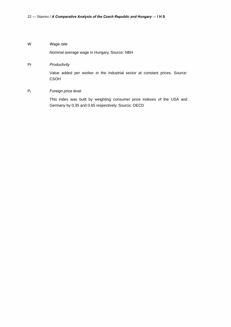
W Wage rate
Nominal average wage in Hungary. Source: NBH
Pr Productivity
Value added per worker in the industrial sector at constant prices. Source:
CSOH
Pf Foreign price level
This index was built by weighting consumer price indexes of the USA and
Germany by 0.35 and 0.65 respectively. Source: OECD
I H S — Stavrev / A Comparative Analysis of the Czech Republic and Hungary — 23
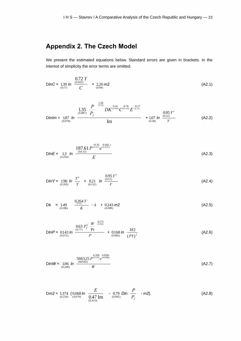
Appendix 2. The Czech Model
We present the estimated equations below. Standard errors are given in brackets. In the
interest of simplicity the error terms are omitted.
DlnC = 1390 17.
( . )ln
0 720 022.
( . )Y
C
+ 2 20
0 94.
( . )m2 (A2.1)
DlnIm = 1870 078.
( . )ln
1350 087
1 260 41 0 76 0 170 55
0 043 0 0.
Im
( . )
.. . .( . )
( . ) ( .116) ( .12)PP
DK C Ef
−
+ 1070 28.
( . )ln
0 950 12.
( . )Y
V
e
(A2.2)
DlnE = 130 254
.( . )
ln187 61
64 15
0 35 0 0420 0 0155.
( . )
. .( .12 ) ( . )P e
E
t−
(A2.3)
DlnY = 1960 265.
( . )ln
YY
e
+ 0 21
0 132.
( . ) ln
0 950 12.
( . )Y
V
e
(A2.4)
Dk = 1490 186.
( . )
0 2640 051.( . )
Y
Kk
e
−
+ 0 243
0 099.
( . )m2 (A2.5)
DlnP = 01430 072.
( . )ln
0 630 77
10 1750 361)
.Pr( . )
.( .
PW
P
f
+ 01680 082.
( . )ln
M
PY
21( )
(A2.6)
DlnW = 1060 249.
( . )ln
5663 25603 82
0 209 0 0390 179 0 0048.
( . )
. .( . ) ( . )P e
W
t
(A2.7)
Dm2 = 13740 229.
( . ) { 0 068
0 079.
( . )ln
E0 470 413. Im
( . )
- 0 79
0 992.
( . )Dln
PPf
- m2}, (A2.8)
24 — Stavrev / A Comparative Analysis of the Czech Republic and Hungary — I H S
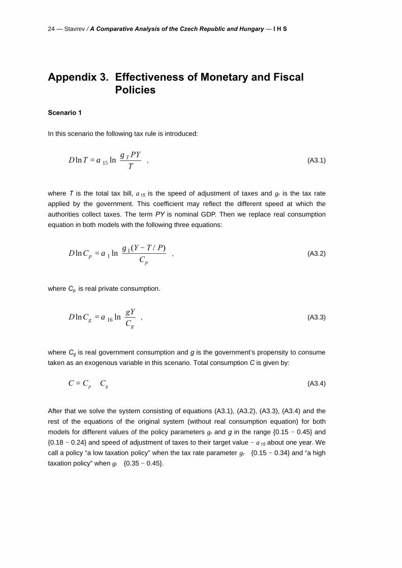
Appendix 3. Effectiveness of Monetary and Fiscal Policies
Scenario 1
In this scenario the following tax rule is introduced:
D TPY
TTln ln=
αγ
15 , (A3.1)
where T is the total tax bill, α15 is the speed of adjustment of taxes and γT is the tax rate
applied by the government. This coefficient may reflect the different speed at which the
authorities collect taxes. The term PY is nominal GDP. Then we replace real consumption
equation in both models with the following three equations:
D CY T P
Cpp
ln ln( / )
=−
α
γ1
1 , (A3.2)
where Cp. is real private consumption.
D CgYCg
g
ln ln=
α 16 , (A3.3)
where Cg is real government consumption and g is the government’s propensity to consume
taken as an exogenous variable in this scenario. Total consumption C is given by:
C C Cp g= + (A3.4)
After that we solve the system consisting of equations (A3.1), (A3.2), (A3.3), (A3.4) and the
rest of the equations of the original system (without real consumption equation) for both
models for different values of the policy parameters γT and g in the range {0.15 − 0.45} and
{0.18 − 0.24} and speed of adjustment of taxes to their target value − α15 about one year. We
call a policy “a low taxation policy” when the tax rate parameter γT ∈{0.15 − 0.34} and “a high
taxation policy” when γT ∈{0.35 − 0.45}.
I H S — Stavrev / A Comparative Analysis of the Czech Republic and Hungary — 25
4.5.2. Scenario 2
In this subsection, a more sophisticated fiscal policy feedback relation is introduced. In both
the Czech and Hungarian models we implicitly assumed that fiscal policy was, in a sense,
neutral and that monetary policy was achieved by reacting to balance of payment variations
and the deviation of domestic inflation from foreign inflation. Here we assume that taxation
rates and government expenditure vary in response to deviations in output from its steady-
state path. The fiscal policy feedback relation can be introduced mathematically by defining
T as follows:
T = γ
γ τ1
1 1g + −( ), (A3.5)
where g is the partial equilibrium ratio of current government expenditure to national income
and τ is the taxation rate. We replace real consumption equation in both models with the
following one
DlnC = α1ln$C
TC
+ α2 m2. (A3.6)
A neutral fiscal policy is obtained if T = 1, in which case equation (A3.6) reduces to the
estimated real consumption equation in both models.
Using equation (A3.5) equation (A3.6) can be rewritten as follows:
DlnC = α1lngY Y T P
C
+ − −
γ τ1 1( )( / ) + α2 m2. (A3.7)
As in the previous case, we introduce the fiscal policy feedback relation into the model by
defining T in the following way:
DlnT = α15 ln( / )*Y Y e
T
ytλ β 20
, (A3.8)
where Y* e λy t is the long run equilibrium growth path of output, and α15 and β20 are policy
parameters. The parameter β20 measures the strength of the feedback. Equation (A3.8)
indicates that lnT depends with an exponentially distributed time lag on the logarithm of the
ratio of real output to its long-run equilibrium level. It also implies that if g is constant, the
taxation rate will converge to a level which increases as the proportional excess of real
26 — Stavrev / A Comparative Analysis of the Czech Republic and Hungary — I H S
output over its long-run level increases. If τ is constant then government propensity to spend
will converge to a level which is lower the greater is the proportional excess of real output
over its long-run equilibrium level. To determine plausible values for this parameter we use
equations (A3.7) and (A3.8). If β20 > 1, then from equation (A3.8) it follows that an increase
in output will allow for an increase in T. In order to increase T the government should
increase taxes and/or decrease spending. It follows from equation (A3.7) that the partial
equilibrium level of aggregate consumption will be less than it would have been if output had
not increased. It is thus unrealistic to assume a value of this coefficient much greater than 1.
The reciprocal of the coefficient α15 is the mean of the distributed time lag with which T
responds to changes in output from its steady-state level. For example α15 = 1 means an
adjustment speed of one quarter.
The new system consisting of the original one plus equation (A3.8) is linearised around the
equilibrium point, and the impact on the stability of the system for different values of the
policy parameters is investigated.
I H S — Stavrev / A Comparative Analysis of the Czech Republic and Hungary — 27
Appendix 4. Anti-inflationary Policies
A4.1. The Effect of Money Supply on Inflation
Dlp
-0.600
-0.400
-0.200
0.000
94Q3 95Q1 95Q3 96Q1 96Q3 97Q1
Figure A4.1 Effect on Prices
Dlrc
-0.240
-0.160
-0.080
0.000
94Q3 95Q1 95Q3 96Q1 96Q3 97Q1
Figure A4.2 Effect on Consumption
DlK
-0.040
-0.030
-0.020
-0.010
0.000
94Q3 95Q1 95Q3 96Q1 96Q3 97Q1
Figure A4.3 Effect on Capital Stock
Dlry
-0.150
-0.100
-0.050
0.000
94Q3 95Q1 95Q3 96Q1 96Q3 97Q1
Figure A4.4 Effect on Output
DlW_P
0.000
0.100
0.200
0.300
94Q3 95Q1 95Q3 96Q1 96Q3 97Q1
Figure A4.5 Effect on Real Wage
Dlre_Dlri
0.000
0.100
0.200
0.300
94Q3 95Q1 95Q3 96Q1 96Q3 97Q1
Figure A4.6 Effect on Trade Balance
28 — Stavrev / A Comparative Analysis of the Czech Republic and Hungary — I H S
A4.2. The Effect of Wages on Inflation
Dlp
-0.300
-0.200
-0.100
0.000
94Q3 95Q1 95Q3 96Q1 96Q3 97Q1
Figure A4.7 Effect on Prices
Dlrc
-0.030
-0.020
-0.010
0.000
0.010
94Q3 95Q1 95Q3 96Q1 96Q3 97Q1
Figure A4.8 Effect on Consumption
DlK
-0.0012
-0.0006
0.0000
0.0006
0.0012
94Q
395
Q1
95Q
396
Q1
96Q
397
Q1
Figure A4.9 Effect on Capital Stock
Dlry
-0.030
-0.020
-0.010
0.000
0.010
0.020
94Q
395
Q1
95Q
396
Q1
96Q
397
Q1
Figure A4.10 Effect on Output
DlW_P
-0.020
0.000
0.020
0.040
0.060
94Q3 95Q1 95Q3 96Q1 96Q3 97Q1
Figure A4.11 Effect on Real Wage
Dlre_Dlri
-0.030
-0.020
-0.010
0.000
0.010
94Q
395
Q1
95Q
396
Q1
96Q
397
Q1
Figure A4.12 Effect on Trade Balance
I H S — Stavrev / A Comparative Analysis of the Czech Republic and Hungary — 29
Appendix 5. Excluding Foreign Prices from Wage Indexation
Dlp
-0.400
-0.200
0.000
94Q
395
Q1
95Q
396
Q1
96Q
397
Q1
Figure A5.1 Effect on Prices
Dlrc
0.000
0.003
0.006
94Q3 95Q1 95Q3 96Q1 96Q3 97Q1
Figure A5.2 Effect on Consumption
DlK
0.0000
0.0050
0.0100
94Q
395
Q1
95Q
396
Q1
96Q
397
Q1
Figure A5.3 Effect on Capital Stock
Dlry
0.000
0.100
0.200
94Q
395
Q1
95Q
396
Q1
96Q
397
Q1
Figure A5.4 Effect on Output
DlW_P
-0.250
-0.150
-0.050 94Q3 95Q1 95Q3 96Q1 96Q3 97Q1
Figure A5.5 Effect on Real Wage
Dlre_Dlri
0.000
0.100
0.200
0.300
94Q3 95Q1 95Q3 96Q1 96Q3 97Q1
Figure A5.6 Effect on Trade Balance
30 — Stavrev / A Comparative Analysis of the Czech Republic and Hungary — I H S
Appendix 6. The Impact of Wage Adjustment
Dlp
-0.400
-0.300
-0.200
-0.100
0.000
94Q
395
Q1
95Q
396
Q1
96Q
397
Q1
Figure A6.1 Effect on Prices
Dlrc
0.000
0.005
0.010
94Q
395
Q1
95Q
396
Q1
96Q
397
Q1
Figure A6.2 Effect on Consumption
DlK
0.000
0.005
0.010
94Q3 95Q1 95Q3 96Q1 96Q3 97Q1
Figure A6.3 Effect on Capital Stock
Dlry
0.070
0.080
0.090
0.100
94Q
395
Q1
95Q
396
Q1
96Q
397
Q1
Figure A6.4 Effect on Output
DlW_P
-0.200
-0.100
0.000
94Q
395
Q1
95Q
396
Q1
96Q
397
Q1
Figure A6.5 Effect on Real Wage
Dlre_Dlri
0.000
0.100
0.200
0.300
94Q3 95Q1 95Q3 96Q1 96Q3 97Q1
Figure A6.6 Effect on Trade Balance
I H S — Stavrev / A Comparative Analysis of the Czech Republic and Hungary — 31
Appendix 7. The Impact of Price and Wage Freeze
Dlp
-0.200
-0.100
0.000
0.100
94Q
395
Q1
95Q
396
Q1
96Q
397
Q1
Figure A7.1 Effect on Prices
Dlrc
-0.020
0.000
0.020
0.040
94Q
395
Q1
95Q
396
Q1
96Q
397
Q1
Figure A7.2 Effect on Consumption
DlK
-0.005
0.000
0.005
0.010
94Q
395
Q1
95Q
396
Q1
96Q
397
Q1
Figure A7.3 Effect on Capital Stock
Dlry
-0.100
0.000
0.100
0.200
94Q3 95Q1 95Q3 96Q1 96Q3 97Q1
Figure A7.4 Effect on Output
DlW_P
-0.200
-0.100
0.000
0.100
94Q
395
Q1
95Q
396
Q1
96Q
397
Q1
Figure A7.5 Effect on Real Wage
Dlre_Dlri
-0.100
0.000
0.100
0.200
94Q
395
Q1
95Q
396
Q1
96Q
397
Q1
Figure A7.6 Effect on Trade Balance
Author: Emil Stavrev
Title: A Comparative Analysis of the Czech Republic and Hungary. – Using Small Continuous-Time
Macroeconometric Models
Reihe Transformationsökonomie / Transition Economics Series 19
Editor: Walter Fisher
Associate Editor: Isabella Andrej
ISSN: 1605-802X
© 2000 by the Department of Economics, Institute for Advanced Studies (IHS),
Stumpergasse 56, A-1060 Vienna • ( +43 1 59991-0 • Fax +43 1 5970635 • http://www.ihs.ac.at

ISSN: 1605-802X