A Comparative Analysis Of Predictive Data-Mining Techniques

A Comparative Analysis

Of

Predictive Data-Mining Techniques

A Thesis

Presented for the

Master of Science Degree

The University of Tennessee, Knoxville

Godswill Chukwugozie Nsofor

August, 2006

ii

DEDICATION

This Thesis is dedicated to my mother

Mrs. Helen Nwabunma Nsofor

Who has gone through thick and

thin without losing faith in what

God can make out of me.

iii

ACKNOWLEDGEMENT

I wish to express my profound gratitude to Dr. Adedeji Badiru, the Head of the

Department of Industrial and Information Engineering, University of Tennessee, for his

fatherly counsel both in and out of schoolwork, and especially for inspiring me towards

completing this thesis work. I lost my biological father, but God has given me a

replacement in him. I thank Dr. Xueping Li in the department of Industrial and

Information Engineering immensely for coming on board to help in advising me to the

completion of this thesis work. I also want to thank Dr. J. Wesley Hines of the

Department of Nuclear Engineering for giving me some of the data sets with which I did

my analysis in this thesis. I also wish to give a big "thank you" to Dr. Robert Ford and

Dr. Charles H. Aikens for agreeing to be part of my thesis committee and for giving me

the necessary tools in their various capacities towards completing this thesis work. My

professors in the Department of Industrial and Information Engineering are unique

people. They are the best anyone can dream of, and I want to thank them immensely for

their investments in my life through this degree in Industrial Engineering.

Femi Omitaomu has been a great brother and friend right from the day I stepped

into the University of Tennessee. I would like to use this opportunity to thank him for all

his assistance to me. I want to use this opportunity to thank my dear and dependable

sister/niece and friend, Rebecca Tasie, for her encouragement and support. She has been

my prayer partner for all these years at the University of Tennessee.

I want to thank Godfrey Echendu and his wife, my spiritual mentor Paul Slay and

his family, my American adopted family of Mr. and Mrs. Ken Glass, and many others

that have played mighty roles in making my stay here in the United States less stressful.

My beloved family at home in Nigeria has always been there for me, staying on

their knees to keep me focused through prayers, especially my younger brother, Dr.

Emmanuel Nsofor.

I pray that the Almighty God will bless you all.

iv

ABSTRACT

This thesis compares five different predictive data-mining techniques (four linear

techniques and one nonlinear technique) on four different and unique data sets: the

Boston Housing data sets, a collinear data set (called "the COL" data set in this thesis), an

airliner data set (called "the Airliner" data in this thesis) and a simulated data set (called

"the Simulated" data in this thesis). These data are unique, having a combination of the

following characteristics: few predictor variables, many predictor variables, highly

collinear variables, very redundant variables and presence of outliers.

The natures of these data sets are explored and their unique qualities defined. This

is called data pre-processing and preparation. To a large extent, this data processing helps

the miner/analyst to make a choice of the predictive technique to apply. The big problem

is how to reduce these variables to a minimal number that can completely predict the

response variable.

Different data-mining techniques, including multiple linear regression MLR,

based on the ordinary least-square approach; principal component regression (PCR), an

unsupervised technique based on the principal component analysis; ridge regression,

which uses the regularization coefficient (a smoothing technique); the Partial Least

Squares (PLS, a supervised technique), and the Nonlinear Partial Least Squares (NLPLS),

which uses some neural network functions to map nonlinearity into models, were applied

to each of the data sets . Each technique has different methods of usage; these different

methods were used on each data set first and the best method in each technique was noted

and used for global comparison with other techniques for the same data set.

Based on the five model adequacy measuring criteria used, the PLS outperformed

all the other techniques for the Boston housing data set. It used only the first nine factors

and gave an MSE of 21.1395, a condition number less than 29, and a modified coefficient

of efficiency, E-mod, of 0.4408. The closest models to this are the models built with all

the variables in MLR, all PCs in PCR, and all factors in PLS. Using only the mean

absolute error (MAE), the ridge regression with a regularization parameter of 1

outperformed all other models, but the condition number (CN) of the PLS (nine factors)

v

was better. With the COL data, which is a highly collinear data set, the best model, based

on the condition number (<100) and MSE (57.8274) was the PLS with two factors. If the

selection is based on the MSE only, the ridge regression with an alpha value of 3.08

would be the best because it gave an MSE of 31.8292. The NLPLS was not considered

even though it gave an MSE of 22.7552 because NLPLS mapped nonlinearity into the

model and in this case, the solution was not stable. With the Airliner data set, which is

also a highly ill-conditioned data set with redundant input variables, the ridge regression

with regularization coefficient of 6.65 outperformed all the other models (with an MSE of

2.874 and condition number of 61.8195). This gave a good compromise between

smoothing and bias. The least MSE and MAE were recorded in PLS (all factors), PCR

(all PCs), and MLR (all variables), but the condition numbers were far above 100. For the

Simulated data set, the best model was the optimal PLS (eight factors) model with an

MSE of 0.0601, an MAE of 0.1942 and a condition number of 12.2668. The MSE and

MAE were the same for the PCR model built with PCs that accounted for 90% of the

variation in the data, but the condition numbers were all more than 1000.

The PLS, in most cases, gave better models both in the case of ill-conditioned

data sets and also for data sets with redundant input variables. The principal component

regression and the ridge regression, which are methods that basically deal with the highly

ill-conditioned data matrix, performed well also in those data sets that were ill-

conditioned.

vi

TABLE OF CONTENTS

CHAPTER PAGE

1.0 INTRODUCTION 1

1.1 STRUCTURE OF THE THESIS 2

1.2 RESEARCH BACKGROUND 3

1.3 TRENDS 5

1.4 PROBLEM STATEMENT 6

1.5 CONTRIBUTIONS OF THE THESIS 6

2.0 LITERATURE REVIEW 8

2.1 PREDICTIVE DATA-MINING: MEANING, ORIGIN AND

APPLICATION 8

2.2 DATA ACQUISITION 11

2.3 DATA PREPARATION 12

2.3.1 Data Filtering and Smoothing 12

2.3.2 Principal Component Analysis (PCA) 15

2.3.3 Correlation Coefficient Analysis (CCA) 18

2.4 OVERVIEW OF THE PREDICTIVE DATA-MINING

ALGORITHMS TO COMPARE 21

2.4.1 Multiple Linear Regression Techniques 23

2.4.2 Principal Component Regression (PCR) 25

2.4.3 Ridge Regression Modeling 27

2.4.4 Partial Least Squares 30

2.4.5 Non Linear Partial Least Squares (NLPLS) 31

2.5 REVIEW OF PREDICTIVE DATA-MINING

TECHNIQUES/ALGORITHM COMPARED 32

2.6 MODEL ADEQUACY MEASUREMENT CRITERIA 34

vii

2.6.1 Uncertainty Analysis 34

2.6.2 Criteria for Model Comparison 36

3.0 METHODOLOGY AND DATA INTRODUCTION 39

3.1 PROCEDURE 39

3.2 DATA INTRODUCTION 41

3.3 DATA DESCRIPTION AND PREPROCESSING 41

3.3.1 Boston Housing Data Set Description and Preprocessing 42

3.3.2 COL Data Set Description and Preprocessing 46

3.3.3 Airliner Data Set Description and Preprocessing 51

3.3.4 Simulated Data Set Description and Preprocessing 55

3.4 UNIQUENESS OF THE DATA SETS 57

4.0 RESULTS AND COMPARISON 59

4.1 THE STATISTICS OR CRITERIA USED IN THE COMPARISON 59

4.2 BOSTON HOUSING DATA ANALYSIS 61

4.2.1 Multiple Linear Regression Models on Boston Housing Data 61

4.2.2 Principal Component Regression on Boston Housing Data 65

4.2.3 Ridge Regression on Boston Housing Data 71

4.2.4 Partial Least Squares (PLS) on Boston Housing Data 77

4.2.5 Nonlinear Partial Least Squares on Boston Housing Data 81

4.3 COL DATA SET ANALYSIS 83

4.3.1 Linear Regressions (MLR) on the COL Data 83

4.3.2 Principal Component Regression (PCR) on the COL data 84

4.3.3 Ridge Regression on the COL Data 91

4.3.4 Partial Least Squares (PLS) on the COL data 95

4.3.5 Non-Linear Partial Least Squares (NLPLS) on the COL Data 98

4.4 THE AIRLINER DATA ANALYSIS 101

viii

4.4.1 Multiple Linear Regression on the Airliner Data 101

4.4.2 Principal Component Regression on the Airliner Data 103

4.4.3 Ridge regression on the Airliner data 108

4.4.4 Partial Least Squares (PLS) on the Airliner data 111

4.4.5 Non-Linear Partial Least Squares on Airliner Data 114

4.5 SIMULATED DATA SET ANALYSIS 116

4.5.1 Multiple Linear Regression on Simulated Data Set 116

4.5.2 Principal Component Regression on Simulated Data Set 118

4.5.3 Ridge Regression on the Simulated data set 122

4.5.4 Partial Least Squares on Simulated Data Set 126

4.5.5 NLPLS on Simulated Data Set 128

5.0 GENERAL RESULTS AND CONCLUSION 131

5.1 SUMMARY OF THE RESULTS OF PREDICTIVE

DATA MINING TECHNIQUES 131

5.1.1 Boston Housing Data Results Summary for

All the Techniques 131

5.1.2 COL Data Results Summary for All the Techniques 133

5.1.3 Airliner Data Results Summary for All the Techniques 133

5.1.4 Simulated Data Results Summary for

All the Techniques 133

5.2 CONCLUSION 137

5.3 RECOMMENDATIONS FOR FUTURE WORK 140

LIST OF REFERENCES 141

APPENDICES 149

VITA 174

ix

LIST OF TABLES

Table 1.1 The three stages of Knowledge Discovery in Database (KDD). 4

Table 2.1 Some of the Applications of Data-Mining 10

Table 2.2 Linear Predictive Modeling Comparison Works 33

Table 4.1 Summary of the results of the three MLR models. 62

Table 4.2 Percentage of Explained Information and the Cumulative Explained 68 Table 4.3 The 14th column of the Correlation Coefficient matrix of

the Boston housing 69 Table 4.4 Summary of All the Results from Principal Component

Regression Models. 70

Table 4.5 Singular Values (SV) for the Boston housing data. 73

Table 4.6 Summary of the Ridge Regression Results on Boston Housing data. 76

Table 4.7 Iterative Method of PLS used to generate MSE for Optimal

Factors selection 78

Table 4.8 Summary of Results Using PLS on Boston Housing data. 79

Table 4.9 Result of the Non-linear Partial Least Squares. 81

Table 4.10 The correlation coefficient matrix of the scores

with output (8th column). 85

Table 4.11 Summary of the MLR Results on the COL data. 86

Table 4.12 Percentage explained information and the cumulative

percentage explained information 88

Table 4.13 Correlation coefficient matrix of the scores with output (13th column). 89

Table 4.14 Summary of the PCR Results on the COL data. 90

Table 4.15 Singular Values (SV) of the COL data. 91

Table 4.16 Summary of the Ridge Regression Results on the COL data Set. 94

Table 4.17 Malinowski's reduced eigenvalues for the COL data 96

Table 4.18 Summary of the PLS Results on the COL data set. 97

Table 4.19 Summary of the NLPLS Results on the COL data. 100

x

Table 4.20 Results from the MLR models. 101

Table 4.21 Percentage explained information and the cumulative explained. 105

Table 4.22 Correlation coefficients of the scores of each PC

with the output variable. 107

Table 4.23 Summary of PCR results on Airliner data. 107

Table 4.24 Singular Value (SV) for the Airliner data. 109

Table 4.25 Summary of Ridge regression results on the Airliner data. 110

Table 4.26 Summary of the PLS results on the Airliner data. 113

Table 4.27 NLPLS results on Airliner data. 115

Table 4.28 Summary of MLR results on the Simulated data set. 118

Table 4.29 Percentage information explained in the PCs

and the cumulative percentage information explained. 121

Table 4.30 Summary of PCR results on Simulated data set. 122

Table 4.31 Singular Values (SV) for the simulated data set. 123

Table 4.32 Summary of ridge regression results on Simulated data set. 125

Table 4.33 Summary of PLS results on simulated data set 127

Table 4.34 Summary of the NLPLS results on Simulated data. 129

Table 5.1 Summary of the Results of the Boston Housing data

for all the techniques. 132

Table 5.2 Summary of the Results of COL data for all the techniques. 134

Table 5.3 Summary of the Results of Airliner Data for All the Techniques. 135

Table 5.4 Summary of the Results of the Simulated data for all the techniques. 136

Table 5.5 Linear models compared with non-linear partial least squares. 138

Table 5.6 Comparison of MLR with PCR, PLS and Ridge regression techniques. 138

Table 5.7 PCR compared with PLS 139

Table 5.8 PLS/PCR compared with Ridge. 139

APPENDICES 149

APPENDIX A

xi

Tables A.1 – A.4 Correlation Coefficient Tables for the four

data sets 150

Table A.5 Malinowski Reduced Eigenvalues for

Boston Housing Data 160

Table A.6 Correlation Coefficients of the Scores of the Simulated

data and the output (Output Column Only) 161

Table A.7 Boston Housing Data set Extract 162

xii

LIST OF FIGURES Figure 1.1 Data-Mining steps. 5

Figure 2.1 The stages of Predictive Data-Mining 9

Figure 2.2 Regression Diagram. 22

Figure 2.3 Schematic Diagram of the Principal Component Regression. 26

Figure 2.4 Schematic Diagram of the PLS Inferential Design. 30

Figure 2.5 Schematic Diagram of the Non Linear Partial Least Squares

Inferential Design. 31

Figure 2.6 Bias-Variance tradeoff and total Uncertainty vs.

the Regularization parameter 'h'. 36

Figure 3.1 Flow Diagram of the Methodology 40

Figure 3.2 A plot of the Boston Housing data set against the index revealing the

dispersion between the various variables. . 43

Figure 3.3 Box plot of Boston Housing data showing the differences in

the column means. 43

Figure 3.4 A plot of the scaled Boston Housing data set against the index

showing the range or dispersion to be between -2 and +2. . 44

Figure 3.5 2-D scores plots of PCs 2 and 1, PCs 2 and 3, PCs 4 and 3,

and PCs 4 and 5 showing no definite pattern between the PCs’ scores 45

Figure 3.6 2D scores plots of PCs 6 and 5, PCs 3 and 5, PCs 7 and 2,

and PCs 6 and 7 showing no definite pattern between the PCs’ scores. 45



Figure 3.8 Plot of the COL data set against the index revealing the dispersion

between the various variables. 47

Figure 3.9 Box plot of the COL data set showing the differences in


Figure 3.10 A plot of the scaled COL data set against the index showing

xiii

the range or dispersion to be between -3 and +3. 48

Figure 3.11 Plots of the score vectors against each other PC2 vs PC1,

PC2 vs PC3, PC4 vs PC3 and PC4 vs PC5; PC2 vs PC1 and PC2 vs PC3

showing some patterns. 49

Figure 3.12 Score vectors of the COL data set plotted against each other. 49

Figure 3.13 2-D scores plots of PCs 8 and 4, PCs 8 and 6, PCs 8 and 7

and PCs 8 and 2. 50

Figure 3.14 2-D scores plots of PCs 8 and 1, PCs 7 and 3, PCs 8 and 3

and PCs 7 and 1 showing no definite pattern between the PCs’ scores 50

Figure 3.15 A plot of the Airliner data set against the index revealing the

Dispersion between the various variables (range of -500 to 4500) 51

Figure 3.16 Box plot of the Airliner data set showing remarkable differences in


Figure 3.17 A plot of the scaled Airliner data set against the index showing a

reduction in the range of the variables (-3 to +3). . 52

Figure 3.18 2-D plots of the score vectors against each other showing no

definite pattern between the PCs’ scores. 53

Figure 3.19 2-D plots of the score vectors showing the relation between

the PCs showing no definite pattern between the PCs’ scores 54

Figure 3.20 2-D plots of the score vectors showing the relation between

the PCs showing no definite pattern between the PCs’ scores. 54

Figure 3.21 Plot of all the variables against the index revealing the level of

dispersion between the variables. 55

Figure 3.22 Box plot of the Simulated data set showing the differences in

the column means (variable means). 56

Figure 3.23 The plot of the scaled data against the index showing a

reduction in the range of the variables (-2 to +3). 56

Figure 3.24 2 -D scores plots of PCs 2 and 1, PCs 2 and 3, and PCs 3 and 1 and

PCs 5 and 4 showing no definite pattern between the PCs’ scores 57


xiv


Figure 3.26 2-D scores plots of PCs 9 and 1, 23 and 21, 18 and 12, 43 and 42

showing no definite pattern between the PCs’ scores . 58

Figure 4.1 Confidence Interval and parameter estimation using stepwise

regression for the Boston Housing data set (MATLAB output).. 63

Figure 4.2 Confidence Interval lines for the training data set prediction

(MATLAB output) for the Boston Housing data set. 63

Figure 4.3 The model-predicted output on the test data outputs for the

Boston Housing data. 65

Figure 4.4 PC Loadings showing the dominant variables in the PCs 1 to 6. 66

Figure 4.5 Loadings for the 7th to 13th principal components showing the

dominant variables in those PCs. 66

Figure 4.6 Scree plot of the eigenvalues vs the PCs. 68

Figure 4.7 The Predicted upon the Test Data Outputs for the Best Two PCR

models. 71

Figure 4.8 Plot of the MSE vs. Alpha for Ridge regression on the


Figure 4.9 Plot of the Regularization Coefficient vs. the Condition Number for

Ridge regression on the Boston Housing data. 73

Figure 4.10 Plot of the Weight vs. the Regularization Coefficient (alpha). 74

Figure 4.11 Norm vs. MSE (L-Curve) for Ridge regression on the


Figure 4.12 Predicted Output over the Original Output of the test data 76

Figure 4.13 Reduced eigenvalues vs. Index. 77

Figure 4.14 MSE vs. Latent Factor Boston Housing Data. 78

Figure 4.15 The predicted plotted upon the original output for nine factors (A)

and 13 factors (B) for the Boston Housing Data. 80

Figure 4.16 Output scores ‘U’ plotted over the input scores ‘T’

(predicted and test response). 80

xv

Figure 4.17 Plot of the Mean Absolute Error vs. latent factors showing

4 optimal latent factors. 81

Figure 4.18 NLPLS Prediction of the test output using four factors for

the Boston Housing Data. 82

Figure 4.19 Output scores over the input scores (predicted and test response). 83

Figure 4.20 Results of the training set used in building the model

(MSE = 28.6867) for the COL data. 85

Figure 4.21 Confidence interval lines for the stepwise regression (COL data) 86

Figure 4.22 Predicted test output plotted on the output test data. 86

Figure 4.23 Loadings of the seven PCs showing the dominant variables

in each PC. 87

Figure 4.24 Scree plot of the eigen values against the number of PCs (COL data) 89

Figure 4.25 PCR predictions on the output data on COL data. 90

Figure 4.26 MSE vs. the Regularization coefficient α. 92

Figure 4.27 Plot of the norm vs. the regularization parameter. 93

Figure 4.28 The L-Curve, norm vs. the MSE for the COL data set. 93

Figure 4.29 Predicted output over the test data output using raw data (A)

and using the scaled data (B). 94

Figure 4.30 Predicted test output over the test data output α = 3.6 (A) and

optimal α =9 (B). 94

Figure 4.31 Plot of the reduced eigenvalues vs. the index. 95

Figure 4.32 Plot of the Mean Square Error vs. the latent factors. 96

Figure 4.33 Predictions of the test output data using: two, four

and all seven factors. 97

Figure 4.34 Output scores over input scores (predicted and test response)

for the COL data. 98

Figure 4.35 Plot of the MAE against the latent factors after the 1st neural

network training. 99

Figure 4.36 Plot of the MAE vs. the latent factors after another neural

network training. 99

xvi


Figure 4.38 Regression coefficients for the training data set in

Stepwise Regression. 102

Figure 4.39 Confidence interval lines for the airliner data set. 102

Figure 4.40 The predicted test output upon the original test outputs. 103

Figure 4.41 The Loadings Vectors vs. the index for the first six PCs. 104

Figure 4.42 Loadings Vectors vs. index for PCs 7 to 12 showing the

dominant variables in each PC. 104

Figure 4.43 Loadings Vectors vs. index for PCs 13 to 18 showing the


Figure 4.44 Scree plot of the Eigenvalues against the PCs for the Airliner data. 106

Figure 4.45 Predicted test output on the original test output. 108

Figure 4.46 MSE vs. Alpha for the Airliner data. 109

Figure 4.47 Norm vs. Alpha for the Airliner data. 110

Figure 4.48 L-Curve for the Airliner data. 110

Figure 4.49 Predicted output over the original output. 111

Figure 4.50 Plot of reduced eigenvalues against the index. 112

Figure 4.51 MSE vs. latent factors used generated from iterative method. 113

Figure 4.52 Predicted output over the original test output for Airliner data. 113


Figure 4.54 Plot of MAE against the latent factors. 115

Figure 4.55 NLPLS scores plotted over the prediction on the Airliner data. 115

Figure 4.56 Output scores over the input scores (predicted and test response)

using NLPLS. 116

Figure 4.57 Confidence interval lines for the training data prediction

(Simulated data set). 117

Figure 4.58 Regression coefficients for the training data in stepwise regression

on the Simulated data. 117

Figure 4.59 The predicted test data output MLR on Simulated data set. 118

Figure 4.60 The loadings of PCs 1 to 6 showing the dominant

xvii

variables in each PC. 119

Figure 4.61 The loadings of PCs 7 to 12 showing the dominant

variables in each PC. 120

Figure 4.62 The loadings of PCs 13 to 18 for the Airliner data showing the


Figure 4.63 Scree plot of the eigenvalues vs. PCs. 121

Figure 4.64 MSE vs. alpha (ridge on Simulated data). 124

Figure 4.65 Weight vs. alpha (ridge on Simulated data). 124

Figure 4.66 Weight vs. MSE (ridge on Simulated data). 125

Figure 4.67 Reduced Eigenvalue vs. Index (PLS on Simulated data). 126

Figure 4.68 MSE vs. latent factors (PLS on Simulated data) generated from

iterative method. 127

Figure 4.69 Output scores over the input scores (predicted and test for the PLS

on Simulated data). 128

Figure 4.70 Mean absolute errors vs. latent factors. 129

Figure 4.71 Internal scores vs. the predicted internal scores

(NLPLS on Simulated data) 129

Figure 4.72 Predicted output on the original output NLPLS on the Simulated data. 130

APPENDIX B

Figure B.1 The predicted output on the Test data Outputs for

the PCR models with 10 PCs and 1st 4 PCs 163

Figure B.2 The predicted output on the Test data Outputs for the PCR

models with 11 PCs and 1st correlation based model, 3PCs

(Boston Housing Data) 163

1

1.0 INTRODUCTION

In recent years, data-mining (DM) has become one of the most valuable tools for

extracting and manipulating data and for establishing patterns in order to produce useful

information for decision-making. The failures of structures, metals, or materials

(e.g.buildings, oil, water or sewage pipes) in an environment are often either a result of

ignorance or the inability of people to take note of past problems or study the patterns of

past incidents in order to make informed decisions that can forestall future occurrences.

Nearly all areas of life activities demonstrate a similar pattern. Whether the activity is

finance, banking, marketing, retail sales, production, population study, employment,

human migration, health sector, monitoring of human or machines, science or education,

all have ways to record known information but are handicapped by not having the right

tools to use this known information to tackle the uncertainties of the future.

Breakthroughs in data-collection technology, such as bar-code scanners in

commercial domains and sensors in scientific and industrial sectors, have led to the

generation of huge amounts of data [1]. This tremendous growth in data and databases

has spawned a pressing need for new techniques and tools that can intelligently and

automatically transform data into useful information and knowledge. For example,

NASA's Earth Observing System, which is expected to return data at the rate of several

gigabytes per hour by the end of the century, has now created new needs to put this

volume of information to use in order to help people make better choices in that area [2].

These needs include the automatic summarization of data, the extraction of the “essence”

of information stored, and the discovery of patterns in the raw data. These can be

achieved through data analyses, which involve simple queries, simple string matching, or

mechanisms for displaying data [3]. Such data-analysis techniques involve data

extraction, transformation, organization, grouping, and analysis to see patterns in order to

make predictions.

2

To industrial engineers, whose work it is to devise the best means of optimizing

processes in order to create more value from the system, data-mining becomes a powerful

tool for evaluating and making the best decisions based on records so as to create

additional value and to prevent loss. The potential of data-mining for industrial managers

has yet to be fully exploited.

Planning for the future is very important in business. Estimates of future values of

business variables are needed. The commodities industry needs prediction or forecasting

of supply, sales, and demand for production planning, sales, marketing and financial

decisions [4]. In a production or manufacturing environment, we battle with the issues of

process optimization, job-shop scheduling, sequencing, cell organization, quality control,

human factors, material requirements planning, and enterprise resource planning in lean

environments, supply-chain management, and future-worth analysis of cost estimations,

but the knowledge of data-mining tools that could reduce the common nightmares in

these areas is not widely available.

It is worthwhile at this stage to state that extracting the right information from a set

of data using data-mining techniques is dependent not only on the techniques themselves

but on the ingenuity of the analyst. The analyst defines his/her problems and goals, has

the right knowledge of the tools available and makes comparative, intuitive tests of which

tool to use to achieve the best result that will meet his/her goals. There are also

limitations for many users of data-mining because the software packages used by analysts

are usually custom-designed to meet specific business applications and may have limited

usability outside those contexts.

1.1 STRUCTURE OF THE THESIS

Chapter One is the introduction of the thesis. It deals with the meaning of data-mining

and some areas where this tool is used or needed. It also covers trends, the problem

statement and the contributions of this thesis. Chapter Two includes a literature review on

data mining, its major predictive techniques, applications, survey of the comparative

analysis by other researchers and the criteria to be used for model comparison in this

3

work. Chapter Three describes the methodology employed in this thesis and an

introduction of the data sets used in the analysis. Chapter Four presents the results and

compares the different methods used in each technique for each data set. Chapter Five

gives a summary of the results, compares the results of the techniques on each data set,

discusses the advantages of each technique over the others, and draws conclusions about

the thesis. This chapter also includes some possible areas for further research.

1.2 RESEARCH BACKGROUND

Berry [5] has classified human problems (intellectual, economic, and business interests)

in terms of six data-mining tasks: classification, estimation, prediction, affinity grouping,

clustering, and description (summarization) problems. The whole concept can be

collectively termed "knowledge discovery." Weiss et al. [6], however, divide DM into

two categories: (a) prediction (classification, regression, and times series) and (b)

knowledge discovery (deviation detection database segmentation, clustering, association

rules, summarization, visualization, and text mining).

Knowledge Discovery in Databases (KDD) is an umbrella name for all those

methods that aim to discover relationships and regularity among the observed data

(Fayyad [3]). KDD includes various stages, from the identification of initial business

aims to the application decision rules. It is, therefore, the name for all the stages of

finding and discovering knowledge from data, with data-mining being one of the stages

(see Table 1.1).

According to Giudici [7], "data mining is the process of selection, exploration,

and modeling of large quantities of data to discover regularities or relations that are at

first unknown with the aim of obtaining clear and useful results for the owner of the

database."

Predictive data mining (PDM) works the same way as does a human handling

data analysis for a small data set; however, PDM can be used for a large data set without

the constraints that a human analyst has. PDM "learns" from past experience and applies

4

Table 1.1 The three stages of Knowledge Discovery in Database (KDD).

this knowledge to present or future situations. Predictive data-mining tools are designed

to help us understand what the “gold,” or useful information looks like and what has

happened during past “gold-mining” procedures. Therefore, the tools can use the

description of the “gold” to find similar examples of hidden information in the database

and use the information learned from the past to develop a predictive model of what will

happen in the future.

In Table 1.1, we can see three stages of KDD. The first stage is data

preprocessing, which entails data collection, data smoothing, data cleaning, data

transformation and data reduction. The second step, normally called Data Mining (DM),

involves data modeling and prediction. DM can involve either data classification or

prediction. The classification methods include deviation detection, database

segmentation, clustering (and so on); the predictive methods include (a) mathematical

operation solutions such as linear scoring, nonlinear scoring (neural nets), and advanced

statistical methods like the multiple adaptive regression by splines; (b) distance solutions,

which involve the nearest-neighbor approach; (c) logic solutions, which involve decision

trees and decision rules. The third step is data post-processing, which is the interpretation,

conclusion, or inferences drawn from the analysis in Step Two. The steps are shown

diagrammatically in Figure 1.1.

Three Stages

1. Data Preprocessing:

• Data preparation

• Data reduction

2. Data Mining:

• Various Data-Mining Techniques

Knowledge Discovery

in Databases (KDD)

3. Data Post-processing:

• Result Interpretation

5

Figure 1.1 Data-Mining steps.

1.3 TRENDS

Because it is an emerging discipline, many challenges remain in data mining. Due to the

enormous volume of data acquired on an everyday basis, it becomes imperative to find an

algorithm that determines which technique to select and what type of mining to do. Data

sets are often inaccurate, incomplete, and/or have redundant or insufficient information. It

would be desirable to have mining tools that can switch to multiple techniques and

support multiple outcomes. Current data-mining tools operate on structured data, but

most data are unstructured. For example, enormous quantities of data exist on the World

Wide Web. This necessitates the development of tools to manage and mine data from the

World Wide Web to extract only the useful information. There has not yet been a good

tool developed to handle dynamic data, sparse data, incomplete or uncertain data, or to

determine the best algorithm to use and on what data to operate.

6

1.4 PROBLEM STATEMENT

The predictive aspect of data mining is probably its most developed part; it has the

greatest potential pay-off and the most precise description [4]. In data mining, the choice

of technique to use in analyzing a data set depends on the understanding of the analyst. In

most cases, a lot of time is wasted in trying every single prediction technique (bagging,

boosting, stacking, and meta-learning) in a bid to find the best solution that fits the

analyst's needs. Hence, with the advent of improved and modified prediction techniques,

there is a need for an analyst to know which tool performs best for a particular type of

data set.

In this thesis, therefore, five of the strongest linear prediction tools (multiple-

linear regression [MLR], principal component regression [PCR]; ridge regression; Partial

Least Squares [PLS]; and Nonlinear Partial Least Squares [NLPLS]), are used on four

uniquely different data sets to compare the predictive abilities of each of the techniques

on these different data samples.

The thesis also deals with some of the data preprocessing techniques that will help

to reveal the nature of the data sets, with the aim of appropriately using the right

prediction technique in making predictions. The advantages and disadvantages of these

techniques are discussed also. Hence, this study will be helpful to learners and experts

alike as they choose the best approach to solving basic data-mining problems. This will

help in reducing the lead time for getting the best prediction possible.

1.5 CONTRIBUTIONS OF THE THESIS

Many people are searching for the right tools to solving predictive data-mining problems;

this thesis gives a direction to what one should do when faced with some of these

problems. This thesis reveals some of the data preprocessing techniques that should be

applied to a data set to gain insight into the type and nature of data set being used. It uses

four unique data sets to evaluate the performances of these five difference predictive data

mining techniques. The results of the performances of the sub-methods on each of the

techniques are compared to each other data set, and finally all the different methods of

each technique are compared with those of other techniques for the same data set.

7

The purpose of this is to identify the technique that performs best for a given type

of data set and to use it directly instead of relying on the usual trial-and-error approach.

When this process is effectively used, it will reduce the lead time in building models for

predictions or forecasting for business planning.

The work in this thesis will also be helpful in identifying the very important

predictive data-mining performance measurements or model evaluation criteria. Due to

the nature of some data sets, some model evaluation criteria may give numbers that seem

statistically significant to a conclusion which, when carefully analyzed, may not actually

be true. An example is the R-squared scores in a highly collinear data set.

8

2.0 LITERATURE REVIEW

This chapter gives the literature review of this research. It explains the various predictive

data-mining techniques used to accomplish the goals and the methods of comparing the

performance of each of the techniques.

2.1 PREDICTIVE DATA MINING: MEANING, ORIGIN AND APPLICATION

Data mining is the exploration of historical data (usually large in size) in search of a

consistent pattern and/or a systematic relationship between variables; it is then used to

validate the findings by applying the detected patterns to new subsets of data [7, 8]. The

roots of data mining originate in three areas: classical statistics, artificial intelligence (AI)

and machine learning [9]. Pregibon [10] described data mining as a blend of statistics,

artificial intelligence, and database research, and noted that it was not a field of interest to

many until recently.

According to Fayyad [11] data mining can be divided into two tasks: predictive

tasks and descriptive tasks. The ultimate aim of data mining is prediction; therefore,

predictive data mining is the most common type of data mining and is the one that has the

most application to businesses or life concerns. Predictive data mining has three stages,

as depicted in Table 1.1. These stages are elaborated upon in Figure 2.1, which shows a

more complete picture of all the aspects of data mining.

DM starts with the collection and storage of data in the data warehouse. Data

collection and warehousing is a whole topic of its own, consisting of identifying relevant

features in a business and setting a storage file to document them. It also involves

cleaning and securing the data to avoid its corruption. According to Kimball, a data ware

house is a copy of transactional or non-transactional data specifically structured for

querying, analyzing, and reporting [12]. Data exploration, which follows, may include the

preliminary analysis done to data to get it prepared for mining. The next step involves

feature selection and or

9

Figure 2.1 The stages of predictive data mining.

reduction. Mining or model building for prediction is the third main stage, and finally

come the data post-processing, interpretation, and/or deployment.

Applications suitable for data mining are vast and are still being explored in many

areas of business and life concerns. This is because, according to Betts [13], data mining

yields unexpected nuggets of information that can open a company's eyes to new

markets, new ways of reaching customers and new ways of doing business. For example,

D. Bolka, Director of the Homeland Security Advanced Research Project Agency

HSARPA (2004), as recorded by IEEE Security and Privacy [14], said that the concept of

data mining is one of those things that apply across the spectrum, from business looking

at financial data to scientists looking for scientific data. The Homeland Security

Department will mine data from biological sensors, and once there is a dense enough

sensor network, there will be enormous data flooding in and the data-mining techniques

used in industries, particularly the financial industry, will be applied to those data sets. In

the on-going war on terrorism in the world especially in the United States of America

10

Table 2.1 Some of the Applications of Data mining.

Application Input Output Business Intelligence

Customer purchase history, credit card information

What products are frequently bought together by customers

Collaborative Filtering

User-provided ratings for movies, or other products

Recommended movies or other products

Network Intrusion Detection

TCPdump trace or Cisco NetFlow logs

Anomaly score assigned to each network connection

Web search Query provided by user Documents ranked based on their relevance to user input

Medical Diagnosis

Patient history, physiological, and demography data.

Diagnosis of patient as sick or healthy

Climate Research

Measurements from sensors aboard NASA Earth observing satellites

Relationships among Earth Science events, trends in time series, etc

Process Mining Event-based data from workflow logs

Discrepancies between prescribed models and actual process executions.

(after Sept. 11th of 2001), the National Security Agency uses data mining in the

controversial telephone tapping program to find trends in the calls made by terrorists with

an aim to aborting plans for terrorist activities. Table 2.1 is an overview of DM's

applications.

In the literature, many frameworks have been proposed for data-mining model

building, and these are based on some basic industrial engineering frameworks or

business improvement concepts. Complex data-mining projects require the coordinated

efforts of various experts, stakeholders, or departments throughout an entire organization

in a business environment; therefore, this makes needful some of the frameworks

proposed to serve as blueprints for how to organize the process of data collection,

analysis, results dissemination and implementing and monitoring for improvements.

These frameworks are CRISP, DMAIC and SEMMA.

1. CRISP steps. This is the Cross-Industrial Standard Process for data mining proposed

by a European consortium of companies in the mid-1990s [15]. CRISP is based on

business and data understanding, then data preparation and modeling, and then on to

evaluation and deployment.

11

2. DMAIC steps. DMAIC (Define-Measure-Analyze-Improve-Control) is a six-sigma

methodology for eliminating defects, waste, or quality-control problems of all kinds

in manufacturing, service delivery, management and other business activities [16].

3. SEMMA steps. The SEMMA (Sample-Explore-Modify-Model-Assess) is another

framework similar to Six Sigma and was proposed by the (Statistical Analysis

System) SAS Institute [17].

Before going into details of the predictive modeling techniques, a survey of the

data acquisition and cleaning techniques is made here. Many problems are typically

encountered in the course of acquiring data that is good enough for the purpose of

predictive modeling. The right steps taken in data acquisition and handling will help the

modeler to get reliable results and better prediction. Data acquisition and handling has

many steps and is a large topic on its own, but for the purpose of this work, only those

topics relevant to this research work will be briefly mentioned.

2.2 DATA ACQUISITION

In any field, even data that seem simple may take a great deal of effort and care to

acquire. Readings and measurements must be done on stand-alone instruments or

captured from ongoing business transactions. The instruments vary from various types of

oscilloscopes, multi-meters, and counters to electronic business ledgers. There is a need

to record the measurements and process the collected data for visualization, and this is

becoming increasingly important, as the number of gigabytes generated per hour

increases.

There are several ways in which data can be exchanged between instruments and

a computer. Many instruments have a serial port which can exchange data to and from a

computer or another instrument. The use of General Purpose Instrumentation Bus (GPIB)

interface boards allows instruments to transfer data in a parallel format and gives each

instrument an identity among a network of instruments [18, 19, 20]. Another way to

measure signals and transfer the data into a computer is by using a Data Acquisition

12

board (DAQ). A typical commercial DAQ card contains an analog-to-digital converter

(ADC) and a digital-to-analog Converter (DAC) that allows input and output to analog

and digital signals in addition to digital input/output channels [18, 19, 20]. The process

involves a set-up in which physical parameters are measured with some sort of

transducers that convert the physical parameter to voltage (electrical signal) [21]. The

signal is conditioned (filtered and amplified) and sent to a piece of hardware that converts

the signal from analog to digital, and through software, the data are acquired, displayed,

and stored. The topic of data acquisition is an extensive one and is not really the subject

of this thesis. More details of the processes can be found in many texts like the ones

quoted above.

2.3 DATA PREPARATION

Data in raw form (e.g., from a warehouse) are not always the best for analysis, and

especially not for predictive data mining. The data must be preprocessed or prepared and

transformed to get the best mineable form. Data preparation is very important because

different predictive data-mining techniques behave differently depending on the

preprocessing and transformational methods. There are many techniques for data

preparation that can be used to achieve different data-mining goals.

2.3.1 Data Filtering and Smoothing

Sometimes during data preprocessing, there may be a need to smooth the data to get rid

of outliers and noise. This depends to a large extent, however, on the modeler’s definition

of "noise." To smooth a dataset, filtering is used. A filter is a device that selectively

passes some data values and holds some back depending on the modeler’s restrictions

[23]. There are several means of filtering data.

a. Moving Average: This method is used for general-purpose filtering for both high and

low frequencies [23, 24, 25]. It involves picking a particular sample point in the

series, say the third point, starting at this third point and moving onward through the

series, using the average of that point plus the previous two positions instead of the

13

actual value. With this technique, the variance of the series is reduced. It has some

drawbacks in that it forces all the sample points in the window averaged to have equal

weightings.

b. Median Filtering: This technique is usually used for time-series data sets in order to

remove outliers or bad data points. It is a nonlinear filtering method and tends to

preserve the features of the data [25, 26]. It is used in signal enhancement for the

smoothing of signals, the suppression of impulse noise, and the preserving of edges.

In a one-dimensional case, it consists of sliding a window of an odd number of

elements (windows 3 and 5) along the signal, replacing the center sample by the

median of the samples in the window. Median filtering gets rid of outliers or noise,

smoothes data, and gives it a time lag.

c. Peak-Valley Mean (PVM): This is another method of removing noise. It takes the

mean of the last peak and valley as an estimate of the underlying waveform. The peak

is the value higher than the previous and next values and the valley is the value lower

than the last and the next one in the series [23, 25].

d. Normalization/Standardization: This is a method of changing the instance values in

specific and clearly defined ways to expose information content within the data and

the data set [23, 25]. Most models work well with normalized data sets. The measured

values can be scaled to a range from -1 to +1. This method includes both the decimal

and standard deviation normalization techniques. For the purpose of this work, the

latter is used. This method involves mean-centering (subtracting the column means

from the column data) the columns of the data set and dividing the columns by the

standard deviation of the same columns. This is usually used to reduce variability

(dispersion) in the data set. It makes the data set have column means of zero and

column variances of one, and it gives every data sample an equal opportunity of

showing up in the model.

i iMC x μ= −

Column mean-centering; MCi has a column means of zero.

ii

MCSCσ

=

14

Column scaling SCi has a column means of zero and variances of 1.

e. Fixing missing and empty values: In data preparation, a problem arises when there are

missing or empty values. A missing value in a variable is one in which a real value

exists but was omitted in the course of data entering, and an empty value in a variable

is one for which no real-world value exists or can be supposed [23, 25]. These values

are expected to be fixed before mining proceeds. This is important because most data-

mining modeling tools find it difficult to digest such values. Some data-mining

modeling tools ignore missing and empty values, while some automatically determine

suitable values to substitute for the missing values. The disadvantages of this process

are that the modeler is not in control of the operation and that the possibility of

introducing bias in the data is high. There are better ways of dealing with missing or

empty values where the modeler is actually in control of which values are used to

replace the missing or empty ones. Two of those will be discussed briefly. Most

importantly, the pattern of the data must be captured. Replacing missing data without

capturing the information that they are missing (missing value pattern) actually

removes the information in the data set. Therefore, unbiased estimators of the data are

used. One of the ways of dealing with missing or empty values is by calculating the

mean of the existing data and replacing the missing values by this mean value. This

does not change or disturb the value of the mean of the eventual data. The other

approach is by not disturbing the standard deviation of the data. This second approach

is generally better than the first because it suggests replacements for the missing

values that are closest to the actual value. Moreover, the mean of the resulting data is

closest to the mean of the data with the right values.

f. Categorical Data: Data-mining models are most often done using quantitative

variables (variables that are measured on a numerical scale or number line), but

occasions do arise where qualitative variables are involved. In this case, the variables

are called categorical or indicator variables [27]. They are used to account for the

different levels of a qualitative variable (yes/no, high/low; or, for more than two

levels, high/medium/low, etc.). Usually, for two different levels, the variable may be

assigned values x = 0 for one level and x = 1 for the other level. For this kind of case,

15

as a general rule, a qualitative variable with r-levels should have r - 1 indicator

variables (or dummy variables). This may lead to some complex scenarios where

there are many interactions between these levels and the quantitative variables. For

these cases, the easiest solution will be to fit separate models to the data for each level

[28]. Computational difficulties arising from the use of these indicator variables can

be eliminated by the use of data-mining software.

g. Dimensionality reduction and feature selection: When the data set includes more

variables than could be included in the actual model building, it is necessary to select

predictors from the large list of candidates. Data collected through computers during

operation usually run through hundreds or thousands of variables. Standard analytic

predictive data-mining methods cannot process data with the number of predictors

exceeding a few hundred variables.

Data reduction is the aggregation or amalgamation of the information contained in

a large data set into manageable information nuggets. Data-reduction methods include

simple tabulation, aggregation, clustering, principal component analysis (PCA) and

correlation coefficient analysis [29]. When there is a reduction in the number of columns,

there is feature reduction and when there is reduction in the number of rows, the sample

points are reduced. For the purpose of this work, only Principal Component Analysis and

correlation coefficient analysis are explained and used.

2.3.2 Principal Component Analysis (PCA)

Principal Component Analysis (PCA) [35] is an unsupervised parametric method that

reduces and classifies the number of variables by extracting those with a higher

percentage of variance in the data (called principal components, PCs) without significant

loss of information [30, 31]. PCA transforms a set of correlated variables into a new set

of uncorrelated variables. If the original variables are already nearly uncorrelated, then

nothing can be gained by carrying out a PCA. In this case, the actual dimensionality of

the data is equal to the number of response variables measured, and it is not possible to

examine the data in a reduced dimensional space. Basically, the extraction of principal

components amounts to a variance maximization of the original variable space. The goal

16

here is to maximize the variance of the principal components while minimizing the

variance around the principal components. The method also makes the transformed

vectors orthogonal [32]. It involves linearly transforming the input variable space into a

space with smaller dimensionality [33].

PCA allows the analyst to use a reduced number of variables in ensuing analyses

and can be used to eliminate the number of variables, though with some loss of

information. However, the elimination of some of the original variables should not be a

primary objective when using PCA.

PCA is appropriate only in those cases where all of the variables arise "on an

equal footing." This means that the variables must be measured in the same units or at

least in comparable units, and they should have variances that are roughly similar in size.

In case the variables are not measured in comparable units, they should be standardized

or normalized (see Section 2.3.1 d) before a PCA analysis can be done. Standardization

will give all variables equal weighting and eliminate the influence of one variable over

the rest. Principal components analysis is perhaps most useful for screening multivariate

data. For almost all data-analysis situations, PCA can be recommended as a first step

[34]. It can be performed on a set of data prior to performing any other kinds of

multivariate analyses. In the process of doing this, new variables (factors) called

principal components (PCs) can be formed in decreasing order of importance, so that (1)

they are uncorrelated and orthogonal, (2) the first principal component accounts for as

much of the variability in the data as possible, and (3) each succeeding component

accounts for as much of the remaining variability as possible. The PCA is computed

using singular value decomposition (SVD) [35], which is a method that decomposes the

X matrix into a unitary matrix U, and a diagonal matrix S that have the same size as X,

and another square matrix V which has the size of the number of columns of X. TX U S V= • •

U = Orthonormal (MxM) matrix of

S = Diagonal (MxN) matrix

where n is the rank of X and the diagonals are known as the singular values and decrease

monotonically. When these singular values are squared, they represent the eigenvalues.

17

V = Orthonormal matrix (NxN) of the eigenvectors, called the loadings vectors or the

Principal Components:

z U S= •

or

z X V= • .

where

Z is an M xN matrix called the score matrix, X is an MxN matrix of original data, and V is

an NxN transformation matrix called the loading matrix. M is the dimensionality of

original space, N is the dimensionality of the reduced PC space, and M is the number of

observations in either space.

This whole process is one of projecting the data matrix X onto the new coordinate

system V, resulting in scores Z. X can be represented as a linear combination of M

orthonormal vectors Vi:

1 1 2 2T T T

M MX z v z v z v= + + +K

Vectors vi are the columns of the transformation matrix V. Each feature zi is a linear

combination of the data x:

1 1 2 2 ,1

n

i i i i n ni j j ij

z xv x v x v x v x v=

= = + + + = ∑K .

It is possible to get the original vector x back without loss of information by transforming

the feature vector z. This is possible only if the number of features equals the dimension

of the original space, n. If k<n is chosen, then some information is lost. The objective is

to choose a small n that does not lose much information or variability in the data. Many

times there is variability in the data from random noise source; this variability is usually

of no concern, and by transforming to a lower dimensionality space this noise can

18

sometimes be removed. The transformation back to the original space can be represented

by important features zi and unimportant or rejected features ri:

1 1

n u

i i i ii i n

x z v r v= = +

= +∑ ∑ .

In the above equation, there are n important features and u - n unimportant

features. The transformation is selected so that the first summation contains the useful

information, and the second summation contains noise [35].

The vectors vi form an orthogonal (actually orthonormal) basis in the PC space.

The basis vectors are chosen to minimize the sum of squared errors between the estimate

and the original data set:

1

n

i ii n

error x z v= +

= − ∑

As shown above, the optimal choice of basis vectors satisfies the following relationship

[33]:

i i iv vλ=∑ .

Again, we recognize this as an eigenvalue problem where λi and vi are the

eigenvalues and eigenvectors of the covariance matrix Σ respectively. The eigenvectors

vi are termed the principal components (PCs) or loadings.

2.3.3 Correlation Coefficient Analysis (CCA)

Correlation coefficient analysis (CCA) [36] assesses the linear dependence between two

random variables. CCA is equal to the covariance divided by the largest possible

covariance and has a range from -1 to +1. A negative correlation coefficient means the

relationship is an indirect one, or, as one goes up, the other tends to go down. A positive

correlation coefficient shows a direct proportional relationship: as one goes up, the other

19

goes up also [21]. The correlation coefficient can be shown with an equation of the

covariance relationship:

If the covariance matrix is given by

⎥⎥⎦

⎤

⎢⎢⎣

⎡= 2

2

),cov(yxy

xyxyxσσσσ

,

the correlation coefficient is:

yx

xyxyp

σσσ

= .

The correlation coefficient function returns a matrix of the following form:

⎥⎦

⎤⎢⎣

⎡=

11

),(xy

xy

pp

yxcorrcoef .

The correlation coefficient ≤ 0.3 shows very little or no correlation (= 0). A correlation

coefficient >3 but <0.7 is said to be fairly correlated. A correlation coefficient ≥ 0.7

shows a high or strong linear relationship. The correlation coefficient of any constant

signal (even with noise) with another signal is usually small. To get a good estimate of

the correlation coefficient, especially for data sets with varying magnitudes, the data

should first be scaled or normalized, or it will give more importance to inputs of larger

magnitude. This is done by dividing each input by the standard deviation of that input as

discussed in Section 2.2 d.

ii

ixx σ=*

20

The covariance matrix of x* equals the correlation matrix of x. This method removes the

dependence of the PCs on the units of measure of the input data. If there are large

variances for certain inputs, then these inputs would dominate the PCs if the covariance

matrix were used [34].

The sample variance (s2) of a probability distribution is a measure of dispersion. If the

mean is known, it is defined as:

( )m

xxs

m

ii

2

12∑=

−= .

The sample covariance (Sjk) assesses the linear dependence between x and y. The

covariance (σj,k) is the average product of ( )( )kikjij xxxx −− . For two unrelated

signals, the covariance is 0 because the negative and positive products cancel each other

out. For two perfectly related signals, the covariance is equal to the product of the

standard deviations (σjk=σjσk); this is the largest possible covariance between two

random variables. Usually the means are not known and the sample covariance is:

( )( )kik

m

ijijkj xxxx

mS −−

−= ∑

= 1, 1

1

where the sample mean is ∑=

=m

iijj x

mx

1

1 .

The data matrix can be written in a zero mean form as X (m x n) where each (i,j)th

element is mean centered ( jij xx − ). The PC score can now be written as

Z X V= •

and the sample covariance is

21

( )( ) XXm

xxxxm

S kik

m

ijijkj '

11

11

1, −

=−−−

= ∑=

.

The variances and covariances of the PC scores (Z) have the same variances and

covariances as those given in the sections above, but the data has a zero mean.

The eigenvectors of [ ] XXm ')1/(1 − are the same as the eigenvectors of

XTX, and the eigenvalues of [ ] XXm ')1/(1 − are 1/ (m-1) times the eigenvalues of

XTX. Because of this, it is sometimes more convenient to calculate the eigenvalues of

XTX rather than those of S. From the foregoing, a matrix of the correlation coefficient of

the input and output variables combined together gives the relationship between the input

and the output. One can reduce the dimension of the matrix by selecting only variables

that are correlated with the predicted variable. This is very useful in feature selection.

Moreover, this correlation coefficient matrix gives the modeler an idea of the collinearity

in the data set.

2.4 OVERVIEW OF THE PREDICTIVE DATA-MINING ALGORITHMS TO

COMPARE

Having discussed the data acquisition, and some data preprocessing techniques, an

overview of the predictive techniques to be compared is given in this section. There are

many predictive data-mining techniques (regression, neural networks, decision tree, etc.)

but in this work, only the regression models (linear models) are discussed and compared.

Regression is the relation between selected values of x and observed values of y from

which the most probable value of y can be predicted for any value of x [32]. It is the

estimation of a real value function based on finite noisy data. Linear Regression was

historically the earliest predictive method and is based on the relationship between input

variables and the output variable. A linear regression uses the dynamics of equation of a

straight line (Figure 2.2) where y = mx + c (m being the slope, c the intercept on the y

axis, and x is the variable that helps to evaluate y). In the case of the linear regression

22

Figure 2.2 Regression Diagram. Showing Data Points and the Prediction Line

model, there is allowance for noise in the relationship and hence we can write the

relationship thus:

y = g(x) + e

where g(x) is equivalent to mx + c, and e represents the noise or error in the model which

accounts for mismatch between the predicted and the actual, while m represents the

weight that linearly combines with the input to predict the output. Most often, the input

variables x are known but the relationship is what the regression modeling tries to

evaluate. When the x variable is multiple, it is known as multiple linear regression.

The term "linear" means that the coefficients of the independent variables are

linear. It might be argued that polynomial models are not linear, but in statistics, only the

parameters, not the independent variables, are considered in classifying the linearity or

nonlinearity of a model. If the parameters (coefficients of the independent variables) are

not linear, then the model becomes nonlinear [37].

In regression analysis, there are some assumptions. These assumptions are

implied throughout this thesis work:

a. A linear relationship is assumed between the input and the output variables [28].

23

b. The error terms ε are random (uncorrelated), normally distributed with mean of zero

and equal or constant variance [28] homoskedasticity [39].

c. Error terms are independent [28, 39]

d. There are few or no outliers [39].

e. There are no interactions or very insignificant interactions between the input variables

[40].

f. The variables are of a known form; in this case first order form [40].

g. The predictors are not correlated [39, 42].

2.4.1 Multiple Linear Regression Techniques

The multiple linear regression model maps a group of predictor variables x to a response variable

y [22, 36]. The equation of the mapping is in the form:

ε+++++= pp xwxwxwxwy ...332211

where wi is the coefficient of the regression. This can also be represented in a matrix

formation, in which case b is equivalent to the intercept on the y axis:

εε +⎥⎦

⎤⎢⎣

⎡=++=

bw

XbXwy *]1[ .

We can solve the above for an optimal weight matrix, wi being the weight or slope. This weight

matrix is optimal when the sum of squares error is minimal (SSE). Below is an estimation of ‘e’,

( ) ( )∑∑ −=−==

nn

iii yySSE 2

1

2ˆ Xwy

where there are n patterns and y is the prediction of y.

24

One assumption made here is that the error term is orthogonal (independent) and

Gaussian (it has a mean of zero and a known variance; other assumptions have been

stated before).

If the X matrix were invertable, it would be easy to solve for w, if the number of

observations equals the number of predictors and the columns are independent (in a square, full-

rank matrix). In normal arithmetic, solving for w can be done using the mathematical equation:

y = xw,

which gives ywx

= .

Since this is usually a matrix formation, a matrix pre-multiplication (pseudo-inverse

solution) is done,

T Tx y x x w= ,

by multiplying both sides by the transpose of x. Then both sides can now be divided by 1( )Tx x − or the inverse of ( )Tx x can be found:

1( )T Tw x x x y−= .

From the equation given, the pseudo-inverse solution was used, where the

inversion of x led to

1( )T Tx x x− .

There may be problems when trying to invert (xTx), especially when the columns are

dependent or marginally dependent. When there is a case of non-invertibility of (xTx) as a

result of dependency among the input variables and the noise (error), an ill-conditioned

25

problem results. When there is marginal dependency of any sort, the problem is ill-posed.

This means that a small perturbation in the data will cause a large perturbation in the

model weights. Moreover, the solutions will not be unique or stable and hence will have a

very high condition number [42]. If the condition number is substantially greater than 1

(>100) [22], the problem is ill-conditioned. If the condition number is under the value 10

conversely, the problem is said to be well conditioned. A condition number between 10

and 100 shows moderately ill-conditioning. Stable problems normally have solutions and

those solutions are unique. Ill-posed problems however, have unrepeatable solutions and

noisy results.

Collinearity is another problem that causes a model to be ill-conditioned.

Collinearity is a situation where the variables are correlated (having high correlation

coefficients) and making the condition number very high. The condition number (CN)

serves the same purpose as variance inflation factor (VIF), Tolerance or condition index

(CI) [43, 44].

There are about three basic methods under this multiple linear regression

technique. There are the full model (which uses the least square approach), the stepwise

regression (discriminant function or all-possible-subsets) [45] and the correlation-based

variable selection [46].

The ultimate aim of every prediction technique is to minimize the term Q, which

is a combination of error and complexity of the model. A widely known maxim is that the

simpler the model the better, and this is true. Hence, a good predictive technique reduces

the dimensionality of the data, reduces the prediction error, and gives a smooth regression

line. Smoothing reduces the weights of the regression coefficients as much as possible

and is the goal.

2.4.2 Principal Component Regression, (PCR)

The second technique is Principal Component Regression (PCR), which makes use of the

principal component analysis [35, 79] discussed in Section 2.3.2. Figure 2.3 is the PCR

transformation, shown diagrammatically. PCR consists of three steps: the computation of

the principal components, the selection of the PCs relevant in the prediction model, and

26

Figure 2.3 Schematic diagram of the Principal Component Regression [22].

the multiple linear regressions. The first two steps are used to take care of collinearity in

the data and to reduce the dimensions of the matrix. By reducing the dimensions, one

selects features for the regression model.

The singular value decomposition of the input variable X was discussed in Section

2.3.2 and can be expressed as

X = U*S*VT.

Transforming to principal components (Figure 2.3),

1 1 2 2T T T

M MX z v z v z v E= + + + +K

or

1 1

n u

i i i ii i n

x z v r v= = +

= +∑ ∑

In this model, zi values are called the score vectors, and the vi are called the loading

vectors, which are the eigenvectors of the covariance matrix of X.

In principal component regression, we overcome the problems that come with performing

regression with collinear data and perform regression with a reduced set of independent

and uncorrelated inputs.

27

When building a regression model using PCA, five methods are available for

selecting the relevant principal components (PCs):

1. Select a number of PCs which has the most variability or most of the information

using the singular values (explained variance) or the eigenvalues [47], or retain only

PCs that correspond to eigenvalues greater than unity [48].

2. From the plot of latent factors or eigenvalues, pick the PCs that are above the kink

(knee) in the plot.

3. Select the PCs that make up to 90% of the information in the model.

4. Select the PCs whose scores (u*s) or (x*v) are correlated with the response variable

called the Best Subset Selection (BSS) [49, 50].

5. Trial and error: One of the flaws of the first four selection criteria is that the explained

variance is not necessarily related to the response variable [51].

Of all the five methods enumerated above, the BSS is the best because it takes into

consideration the relationship of the predictor variables x with the predicted variable y.

The correlation coefficient between the scores of the PCs (U*S or X*V) and the response

variable y is computed, and the variables with the strongest correlations are used to build

the model. The correlation coefficients are values sorted out by their absolute values

(irrespective of sign) and the PCs are entered in this order. It may interest the modeler to

transform back into the original X transformation with the elimination of features (PCs)

that are irrelevant for the best prediction before performing the regression analysis.

2.4.3 Ridge Regression Modeling

The ridge regression technique [52, 53, 83] is very similar to the pseudo-inverse solution

discussed in Section 2.4.1, but it adds the product of squared alpha and an identity matrix

(α2*I) in the xTx matrix to make it invertable. It shrinks the regression coefficients by

imposing a penalty on their size [54]. The addition of the product of squared alpha and an

identity matrix is called regularization, and alpha is the regularization parameter or ridge

coefficient:

28

2 1( )T Tw X X I X yα −= + .

This parameter controls the trade-off between the smoothness of the solution and the

fitness of the data. The ridge technique is called the smoothing technique because it is

characterized by reducing the weights, in turn reducing the condition number. The ridge

equation for condition number reduction is given below.

Without regularization coefficient "alpha", condition number =2max2min

SS

,

but with alpha, Condition number = 2 2max2 2min

SS

αα++

.

This is also very similar to the principal component regression technique in that it

chooses the number of relevant PCs. The regularization parameter is related to the

singular values. The optimum α value is slightly smaller than the least significant

principal component that will go into the model (least significant singular value).

The regularization operation is also related to the weight by

1*

ni

ii i

i

b vβασ σ=

=+

∑ ,

where βi = uiTY.

Small weights give a smooth solution [21]. If σi is greater than α, then regularization has

little effect on the final least-square solution. If σi is less than α, then the corresponding

term in the solution can be expressed as

29

*i i ii i

ii

v vβ σ βα ασ σ=

+,

and this term approaches 0 as σi tends to 0.

Making alpha (the regularization coefficient) larger helps to reduce the weight of the

regression coefficients. This result is one of the benefits of ridge regression.

In selecting the alpha value, any of these criteria can be used: Morozov’s Discrepancy

Principle [55]; Mallows’ CL Method [56]; Press LOOCV [57]; Generalized Cross

Validation [58]; or the L-Curve [21].

The L-Curve is a plot of the residual norm versus the solution norm. The residual

norm is composed of error that cannot be reduced by the model and bias due to

regularization. The solution norm is a measure of the size of the regression coefficients or

weights of the regression coefficients. As the regularization parameter (α) is increased,

weights or regression coefficients become smaller, making the solution smoother but also

adding bias to the solution. The best solution is found at a point just below the curve

where there is compromise in the error. This point gives the optimal regularization

parameter α. This method is simple and reliable.

In kernel regression [38], Tikhonov’s regularization [59, 60, 61] places the

roughness penalty directly onto the sought function, while the ridge technique places the

penalty on the weights (w):

Min{||Ax - b||22 + λw2}.

30

2.4.4 Partial Least Squares

Another predictive data-mining technique is the Partial Least Squares (PLS) [62]. PLS is

a method of modeling input variables (data) to predict a response variable. It involves

transforming the input data (x) to a new variable or score (t) and the output data (y) to a

new score (u) making them uncorrelated factors and removing collinearity between the

input and output variables. A linear mapping (b) is performed between the score vectors t

and u (see Figure 2.4). The score vectors are the values of the data on the loading vectors

p and q. Furthermore, a principle component-like analysis is done on the new scores to

create loading vectors (p and q).

Figure 2.4, an inferential design of PLS by Hines [22], is a representation of this.

In contrast to principal component analysis (PCA), PLS focuses on explaining the

correlation matrix between the inputs and outputs but PCA dwells on explaining the

variances of the two variables. PCA is an unsupervised technique and PLS is supervised.

This is because the PLS is concerned with the correlation between the input (x) and the

output (y) while PCA is only concerned with the correlation between the input variables

x.

As can be seen in Figure 2.4, b would represent the linear mapping section

between the t and u scores. The good point of PLS is that it brings out the maximum

amount of covariance explained with the minimum number of components. The number

of latent factors to model the regression model is chosen using the reduced eigenfactors.

The eigenfactors are equivalent to the singular values or the explained variation in the PC

selection and are normally called the Malinowski’s reduced eigenvalue [63]. When the

reduced eigenvalues are basically equal, they only account for noise.

Figure 2.4 Schematic diagram of the PLS Inferential Design.

31

2.4.5 Non Linear Partial Least Squares (NLPLS)

The NLPLS [64, 65] is essentially the same as the PLS; it involves transforming the input

data (x) to a new variable or score (t) and the y data to a new score (u), making them

uncorrelated factors and removing collinearity between the input and output variables.

This is shown diagrammatically in Figure 2.5, an inferential design of NLPLS by Hines

[22]. It is just the same as the process explained above, with the major difference being

that in the linear PLS method, the inner relationships are modeled using simple linear

regression.

The difference between PLS and the NLPLS models is that in NLPLS, the inner

relationships are modeled using neural networks [73, 67]. For each set of score vectors

retained in the model, a Single Input Single Output (SISO) neural network is required

[22]. These SISO networks usually contain only a few neurons arranged in a two-layered

architecture. The number of SISO neural networks required for a given inferential

NLPLS unit is equal to the number of components retained in the model and is

significantly less than the number of parameters included in the model [32].

Figure 2.5 Schematic diagram of the Non Linear Partial Least Squares Inferential

Design.

32

2.5 REVIEW OF PREDICTIVE DATA MINING TECHNIQUES/ALGORITHMS

COMPARED

The problem of choice of modeling technique comes up when a data analyst is given new

sets of data of which he has no knowledge or background. Selection of the best technique

to perform the data analysis in all cases requires the analyst to have a deep understanding

of all the modeling techniques with their advantages and disadvantages and a reasonable

knowledge of the nature of the measured data to be analyzed and the process being

modeled [66]. In his work, Bhavik [66] did a comparison of the three broad categories of

predictive data-modeling methods: linear statistical methods, artificial neural network and

nonlinear multivariate statistical methods. Munoz et al. [67] compared logistic multiple

regression, principal component regression (PCR) and classification and regression tree

analysis (CART) with the multivariate adaptive regression splines (MARS). Manel et al.

[68] compared discriminant analysis, neural networks and logistic regression for

predicting species distributions. Frank et al. [69] examined Partial Least Squares (PLS)

and principal component regression and compared the two with ridge, variable subset

selection and ordinary least squares.

Among these predictive data-mining methods, a lot of work has been done on the

linear predictive modeling methods (see Table 2.2). The connections between these linear

models have been studied [70, 71].

In their work, Elder et al. [72] did a comprehensive comparison of the different

data-mining tools (software) available now. The tools evaluated are Clementine (version

4), Darwin (version 3.0.1), Datacruncher (version 2.1.1), Enterprise Miner (version Beta),

GainSmart (version 4.0.3), Intelligent Miner (version 2), Mineset (version 2.5), Model 1

(version 3.1), ModelQuest (version 1), PRW (version 2.1), CART (version 3.5),

NeuroShell (version 3), OLPARS (version 8.1), Scenario (version 2), See5 (version

1.07), S-Plus (version 4), and WizWhy (version 1.1). These softwares were compared

according to the platform supported by the different software packages, the algorithms

included in the software packages, data input and model output options, usability ratings,

visualization capabilities and model automation.

33

Table 2.2 Linear Predictive Modeling Comparison Works

SN Author/year Work Result Comparison Measure

1 Orsolya et.al [80], 2005.

Compared Ridge, PLS, Pair-wise Correlation Method (PCM), Forward Selection (FS), and Best Subset Selection (BSS) on a quantitative structure-retention relationship (QSSR) study based on multiple linear regression on prediction of retention indices for aliphatic alcohols.

PCM gave a more reliable result than others

MSE, R2, PRESS, F

2 Huang, J. et.al [81], 2002.

Compared Least square Regression, Ridge and PLS in the context of the varying calibration data size using only squared prediction errors as the only model comparison criterion.

The results depended on the type of data set and the data size.

Average RMSE, 95 percentile RMSE

3 Vigneau, E. et.al [82], 1996.

Compared ridge, PCR and ordinary least square regression with ridge principal component, RPC (blend of ridge and PCR) on the bases of two data sets.

RPC performed well

PRESS, MSE

4 Malthouse, C. E. et.al [83], 2000.

Compared ridge with stepwise regression on direct marketing data.

Ridge provides amore stable way of moderating degrees of freedom than dropping variables.

MSE

5 Basak, C. Subhash et.al [84], 2003.

Used PCR, PLS, ridge to develop quantitative structure-activity/property relationship (QSAR/QSPR) models for the estimation of human blood: air partition coefficient.

Ridge regression was found to be superior.

6 Naes, T. and Irgens, C. [85], 1985

Compared MLR, ridge, PCR, and PLS on near infrared instrument statistical calibration.

Ridge, PCR and PLS gave better predictions.

RMSE

34

2.6 MODEL ADEQUACY MEASUREMENT CRITERIA

In comparing the performance of these different prediction techniques, some quantities

that interpret the goodness of fit of a model, and error measurements will be discussed in

this section. There are also factors that affect the complexity of the model and increase its

uncertainty, determining to a large extent the predictability of the model. This will also be

discussed here.

2.6.1 Uncertainty Analysis

A good prediction technique is one that works to reduce the uncertainty of the model. The

uncertainty of a model is measured by:

Uncertainty = Variance + Bias2.

A number of factors increase the uncertainty of a model:

a. Information Selection: The addition of unnecessary inputs to the model increases the

solution variance, and not having enough necessary input also increases the bias of

the model.

b. Choice of Model: The choice of the technique plays a large role in the uncertainty of

a model. When nonlinear data are fitted to a linear model, the solution is usually

biased. When linear data are fitted to a nonlinear model, the solution usually increases

the variance. Using principal component analysis, one can determine if the given

information can be modeled by a linear or a nonlinear technique. This can be found

by plotting the different principal components (score vectors) of the whole data

matrix, including the dependent variables, against each other. Since different

principal components for a linearly related model are expected to be independent and

perpendicular to each other, the results should show scatter plots for each pair of

combination of the principal components. This is an indication that the relationship

between the variables is linear. If the plots of the different PCs show regular patterns

(a curve or a straight line), it is an indication of the existence of nonlinear relationship

in the model.

35

c. Proper complexity through regularization: A complex model is one in which the

events are mostly described as random or without pattern. It takes many bits of

information to represent them, and yet they do not have a pattern. Since a complex

model has random events, its uncertainty is high, and it is difficult to understand its

pattern. The essence of regularization is to stabilize the solution with respect to

variations in the data. This is known as variance-bias tradeoff, and it ends in reducing

the variance to the barest minimum while keeping the bias at its lowest possible

range. When a complex model is under-regularized, the data is over-fit and this

increases the variance, but when the model is over-regularized, it is over-smoothed,

and the bias increases (Figure 2.6). The essence of regularization is to reduce the

MSE. A well regularized model will reduce the variance of the model and give a

more consistent and repeatable result, with no bias. Figure 2.6 (from Monitoring and

Diagnostic class note [22]) shows what happens on regularization. As the

regularization parameter 'h' is increased, the variance of the model decreases; the

uncertainty at this point also decreases. This decrease in variance continues up to a

point where the uncertainty becomes minimum; at this point, the bias of the model

becomes significant. As the regularization parameter continually increases, the bias

contribution becomes very significant, and this conversely causes uncertainty to

increase, even as the variance continues to decrease [61].

d. Another cause of uncertainty is the presence of noise. As mentioned above, noisy data

do not have a pattern. Noise in the training and response variables cause an increase

in uncertainty.

e. Uncertainty is affected by the quantity of data available for building the model. If the

quantity of data, is large, there is a better chance of making a good model. The less

data available, the more uncertain it will be that one can get a good representation of

the model. The quantity of data can bring about over-fitting and or inclusion of

unnecessary information in the model, increasing the mean square error.

f. Training Region: Finally, the uncertainty of a model is also affected by the ability of

the training data to cover the operating regions. This is true because if the training

36

Figure 2.6 Bias-Variance Tradeoff and Total Uncertainty vs. the Regularization

Parameter 'h'.

data set does not cover the whole operating region, the model will not give a good

representation of the available information.

2.6.2 Criteria for Model Comparison

Many criteria can be used to evaluate the predictive abilities of the different DM

techniques. For the purpose of this work, about nine criteria will be used in comparing

different methods within each technique but these five criteria will be used to compare

the different techniques: mean square error (MSE), mean absolute error (MAE),

condition number (CN) [42] / the weight of the regression coefficients, the number of

variables of features included in the model, and the modified coefficient of efficiency.

a. Mean Square Error (MSE): The first and most significant criterion for comparing the

predictive abilities of the different DM techniques is the mean square error or MSE.

The MSE of the predictions is the mean of the squares of the difference between the

observed values of the dependent variables and the values of the independent

37

variables that would be predicted by the model. It is the mean of the squared

difference between the observed and the predicted values or the mean square of the

residuals. MSE can reveal how good the model is in terms of its ability to predict

when new sets of data are given. A high value of MSE is an indication of a bad fit. A

low value is always desirable. Outliers can make this quantity larger than it actually

is. MSE gives equivalent information as R-square adjusted (R2adj.).MSE has an

advantage over some process capability indexes because it directly reflects variation

and deviation from the target. [74]

b. The condition number [42]/weight of the regression coefficients: After a model is

constructed, the weight of the regression coefficients can tell how good the model is.

If there are unnecessary inputs in the data, the weights of the regression coefficients

increase. This is may be seen by the value of the condition number of the data matrix

(see section 2.4.1). Though the model itself may show very little mean square error,

the bias is high, which increases the uncertainty of the model. It has been mentioned

that one of the consequences of increased uncertainty in a model is the inconsistency

of the result, meaning that it is not repeatable or unrealistic; this is caused by the high

condition number.

c. The number of variables or features included in the model: The number of variables

included in a model determines how good the model will be. A good predictive DM

technique accounts for most of the information available. It builds a model that gives

the most possible information representative of the system being predicted with the

least possible MSE. However, when more features are added, the mean square error

tends to increase. The addition of more information added increases the probability of

adding irrelevant information into the system. A good DM model selects the best

features or variables that will account for the most information needed to explain or

build the model.

In most cases, the rule of Occam's Razor, which states that the simpler

explanation is the preferable one, is very useful. This idea originated from a

theological principle stated by William of Occam, a Franciscan monk (1280), and is

now applied to data analysis or DM techniques in building models. A data analyst

38

should strive to build a model with the smallest number of features that can explain

the most basic information or reduce the number of causes to a bare minimum [75].

d. Coefficient of Efficiency: This has been used in many fields of science for evaluating

model performance [76,, 77, 78]. According to Nash et al. [77], the coefficient of

efficiency can be defined as

2

1

2

1

( )1 1

_ _( )

n

i ii

n

ii

O XMSEE

Variance of ObservedO X

=

=

−= − = −

−

∑

∑.

The ratio of the mean square error to the variance of the observed data is subtracted

from unity. It ranges from -1 to +1, where -1 indicates a very bad model, since the

observed mean is a better predictor than the predicted variables. A value of zero

would show that observed mean is as good as the predicted model.

e. Mean absolute error (MAE): This measurement is the summation of the absolute

values of the errors (difference between the predicted and the prediction). MAE has

an advantage over MSE because it takes care of over-estimation due to outliers. Using

MSE, a data set that has a lot of outliers gets bloated when they are squared, and this

affects the resulting numbers even when the square root is computed.

39

3.0 METHODOLOGY AND DATA INTRODUCTION

In this chapter, the methodology used in this thesis work is described. This is the

procedure used in evaluating the various predictive data mining techniques using the four

different and unique data sets. This chapter also deals with the introduction and

description of the four data sets used in this study, using preliminary diagnoses to check

for the relationships between the variables in each data set and to visualize the nature or

properties of the data sets.

3.1 PROCEDURE

Figure 3.1 shows a diagram of the methodology used in this thesis work. The four data

sets are first introduced, as well as the preliminary diagnoses done on each data set to

gain an insight into their properties. The relationship check is made by plotting the inputs

over the output of the raw data sets. The data is preprocessed by scaling or standardizing

them (data preparation) to reduce the level of dispersion between the variables in the data

set. The correlation coefficients of each of the various data sets are computed to verify

more on the relationship between the input variables and the output variables. This is

followed by finding the singular value decomposition of the data sets transforming them

into principal components. This also will be helpful in checking the relationship between

the variables in each data set.

At this stage, the data sets are divided into two equal parts, setting the odd number

data points as the "training set" and the even number data points as the "test validation

data set." Now the train data for each data set is used for the model building. For each

train

40

Figure 3.1 Flow Diagram of the Methodology

data set, a predictive data mining technique is used to build a model, and the various

methods of that technique are employed. For example, Multiple Linear Regression has

three methods associated with it in this thesis: the full model regression model, the

stepwise regression method, and the model built selecting the best correlated variables to

the output variables. This model is validated by using the test validation data set. Nine

model adequacy criteria are used at this stage to measure the goodness of fit and

adequacy of the prediction. The results are presented in tables. The results of the train

sets are not presented in this study because they are not relevant. This is because only the

performance of the model on the test data set or entirely different (confirmatory) data set

is relevant. The model is expected to perform well when different data sets are applied to

it. In this thesis work, the unavailability of different but similar real-life data sets has

limited this study to using only the test data set for the model validation. This is not a

serious problem since this work is limited to model comparison and is not primarily

concerned with the results after deployment of the model.

41

Finally, all the methods of all the techniques are compared (based on their results on

each data set) using four very strong model adequacy criteria. The best result gives the

best prediction technique or algorithm for that particular type of data set.

3.2 DATA INTRODUCTION

Four different and unique data sets are used in this work. They include the Airliner data

set [86], the COL data set [22], the Boston Housing data set, and the Simulated data set

[86]. Only the Boston Housing data set, obtained from http://lib.stat.cmu.edu/datasets/,

has its variables described in detail. For the purpose of this work, MATLAB software

was used for all of the analyses. These data sets have all at some stage in the analyses

been prepared before being used for the analyses (Section 2.3).

Before any of these techniques were used on the data sets, preliminary analyses

were done on the data sets to gain at least a superficial knowledge of the data sets or to

see the nature of the data sets. In real-life analysis, this preliminary data description is an

important step in data-mining because in most cases, it helps the analyst in making a

choice of the techniques to be used in the regression work.

3.3 DATA DESCRIPTION AND PREPROCESSING

The plots of all the variables in each data set against the indices were made to see the

measure of dispersion between the different variables. The plots of the input variables

against the output variable for each data set were made to gain a superficial knowledge of

the relationship between the input variables and the output variables of the data sets. The

correlation coefficients of the data matrix were calculated to see how the variables

correlated with each other. To check if the variables had nonlinear relationships, the

singular value decomposition of the data sets were evaluated. The score vectors were

plotted against each other (for each data set) to check for the presence of nonlinear

relationships between the variables.

42

3.3.1 The Boston Housing Data Set Description and Preprocessing

The Boston data set was obtained from the StaLib archive at

http://lib.stat.cmu.edu/datasets/boston. See Appendix A.7 for an extract. This data set

contains information collected by the U.S Census Service concerning housing in the area

of Boston, Massachusetts. The data consist of 14 variables or features and 506 data

points. For this thesis, the 14 features were divided into two: 13 independent variables

and 1 dependent variable. These features, numbered according the column numbers

included:

1. Per capita crime rate by town (CRIM)

2. Proportion of residential land zoned for lots over 25,000 sq. ft. (ZN).

3. Proportion of non-retail business acres per town (INDUS).

4. Charles River dummy variable (1 if tract bounds river; 0 otherwise) (CHAS).

5. Nitric Oxide concentration (parts per 10 million) (NOX).

6. Average number of rooms per dwelling (RM).

7. Proportion of owner-occupied units built prior to 1940 (AGE).

8. Weighted distances to five Boston employment centers (DIS).

9. Index of accessibility to radial highways (RAD).

10. Full value property tax per $10,000 (TAX).

11. Pupil-teacher ratio by town (PTRATIO).

12. 1000*(Bk – 0.63)2 where Bk is the proportion of African-American residents by town

(B).

13. Percentage lower status of the population (LSTAT).

14. Median value of the owner-occupied homes in $1000's (Mval).

Variable 14 in this case is the response variable. The rest are independent variables.

Figure 3.2 reveals the measure of dispersion between the 14 variables of the data set. It

ranged from almost 0 to about 700 units. Figure 3.3 is a box plot of the data set and

throws more light on the measure of dispersion between these variables, comparing the

means of the various columns (the dashed line in the rectangular boxes). It also helped to

43

Figure 3.2 A plot of the Boston Housing data set against the index revealing the

dispersion between the various variables.

Figure 3.3 Box plot of Boston Housing data showing the differences in the means of

the variables.

44

Figure 3.4 A plot of the scaled Boston Housing data set against the index showing

the range or dispersion to be between -2 and +2.

identify the outliers in each variable or column. To bring out all the features or

information in each variable, the data set was scaled, giving every variable equal

opportunity of bringing out its information as contained in the data. The data set now had

a column mean of 0 and a standard deviation of 1. Plotting it against the index again gave

Figure 3.4. Note: spikes in Figure 3.4 were results of noise or outliers.

Some of the variables tend to have no direct correlation (see Table A.1 in the Appendix)

with the output variable (Median Value of the owner-occupied homes in $1000's). From

that table, it can be deduced from Column 14 that most of the variables either have weak

correlation with the output variable or are negatively correlated with it. Table 4.3 in

Chapter Four shows the 14th column of the correlation coefficient matrix of the Boston

Housing data set. The full correlation coefficient matrix of the Boston data is shown in

Appendix Figure A.1.

From the score vector plots in Figures 3.5, 3.6 and 3.7, it can be seen that the PCs plotted

against each other show a scatter plot. This might be an indication that the relationship

between these variables is a linear one. When the score vectors are plotted against each

other, it shows a definite pattern, either a straight line or a curve; it shows that the

variables have a relationship other than a linear one.

45

Figure 3.5 2-D scores plots of PCs 2 and 1, PCs 2 and 3, PCs 4 and 3, and PCs 4 and

5, showing no definite pattern between the PCs' scores.

Figure 3.6 2D scores plots of PCs 6 and 5, PCs 3 and 5, PCs 7 and 2, and PCs 6 and

7, showing no definite pattern between the PCs' scores.

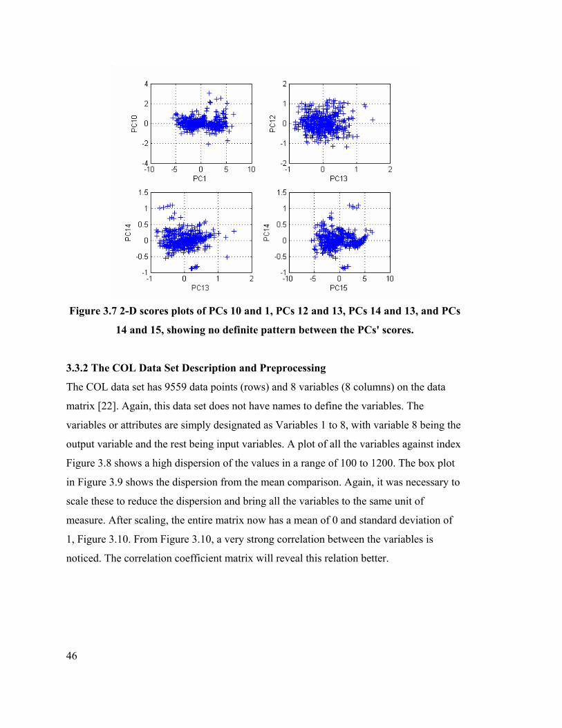
46

Figure 3.7 2-D scores plots of PCs 10 and 1, PCs 12 and 13, PCs 14 and 13, and PCs

14 and 15, showing no definite pattern between the PCs' scores.

3.3.2 The COL Data Set Description and Preprocessing

The COL data set has 9559 data points (rows) and 8 variables (8 columns) on the data

matrix [22]. Again, this data set does not have names to define the variables. The

variables or attributes are simply designated as Variables 1 to 8, with variable 8 being the

output variable and the rest being input variables. A plot of all the variables against index

Figure 3.8 shows a high dispersion of the values in a range of 100 to 1200. The box plot

in Figure 3.9 shows the dispersion from the mean comparison. Again, it was necessary to

scale these to reduce the dispersion and bring all the variables to the same unit of

measure. After scaling, the entire matrix now has a mean of 0 and standard deviation of

1, Figure 3.10. From Figure 3.10, a very strong correlation between the variables is

noticed. The correlation coefficient matrix will reveal this relation better.

47

Figure 3.8 Plot of the COL data against the index showing the dispersion between

all the variables.

Figure 3.9 Box plot of the COL data set showing the differences in the means of the

variables.

48

Figure 3.10 A plot of the scaled COL data set against the index showing the range or

dispersion to be between -3 and +3.

The correlation coefficient matrix is shown below in Appendix Table A.2. From

the correlation coefficient matrix, it can be observed that all the variables are strongly

correlated with each other. Indeed, they are almost perfectly correlated with each other

and with the response variable.

The score vector plots, Figure 3.11 and 3.12 show both regular and irregular

patterns. Plots of PC1 and PC2, PC2 and PC3 in Figure 3.13, PC7 and PC2 in Figure

3.12, PC8 and PC2 in Figure 3.13 indicate that perhaps there may be nonlinear

relationships between these variables. The plots in Figure 3.14 show no definite pattern.

Therefore there is no nonlinear relationship between those PCs' scores plotted. This will

further be revealed from the plot of inner scores matrix and outer score matrix of the

Partial Least Square model and that of the Nonlinear Partial Least Squares in Chapter

Four.

49

Figure 3.11 Plots of the score vectors against each other: PC2 vs PC1, PC2 vs PC3,

PC4 vs PC3 and PC4 vs PC5; PC2 vs PC1 and PC2 vs PC3 showing some patterns.

Figure 3.12 Score vectors of the COL data set plotted against each other.PC6 vs

PC5, PC3 vs PC5, PC7 vs PC2 and PC6 vs PC7; with PC7 vs PC2 showing a

pattern.

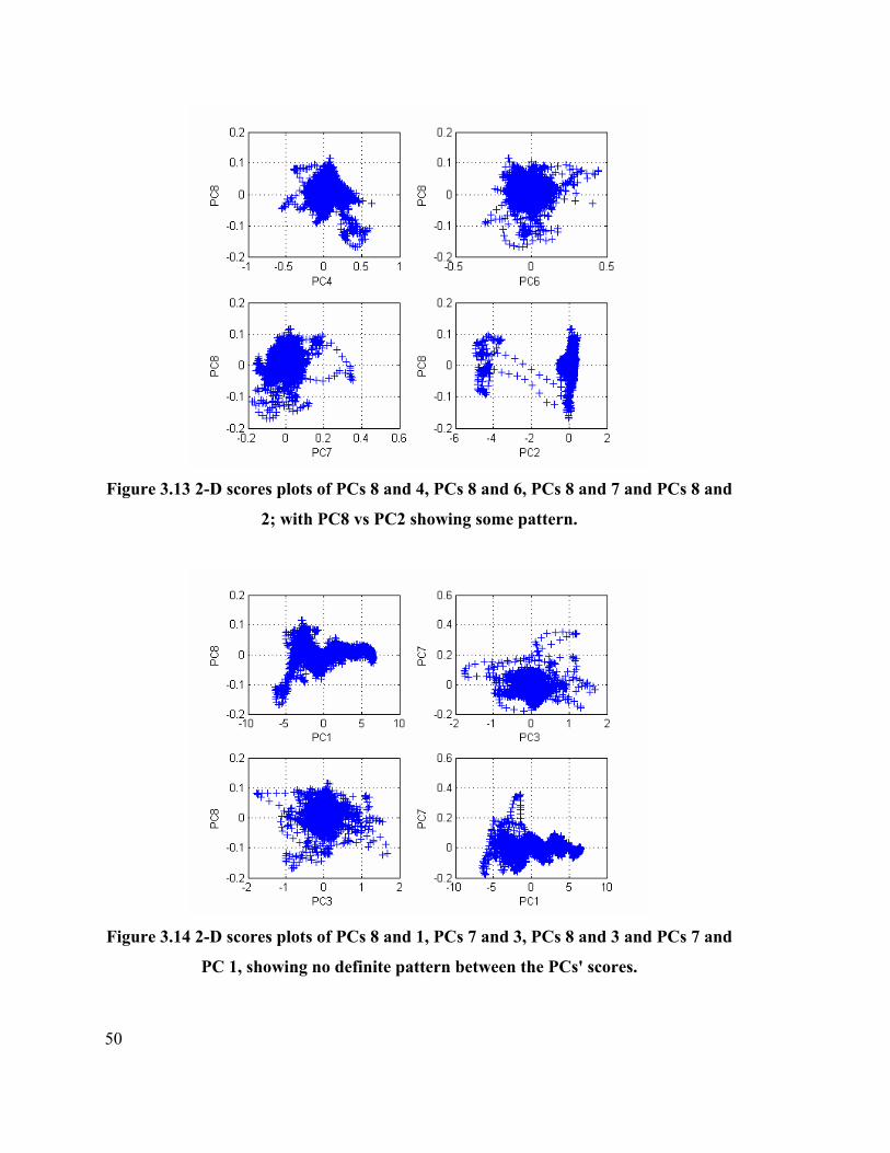
50

Figure 3.13 2-D scores plots of PCs 8 and 4, PCs 8 and 6, PCs 8 and 7 and PCs 8 and

2; with PC8 vs PC2 showing some pattern.

Figure 3.14 2-D scores plots of PCs 8 and 1, PCs 7 and 3, PCs 8 and 3 and PCs 7 and

PC 1, showing no definite pattern between the PCs' scores.

51

3.3.3 The Airliner Data Set Description and Preprocessing

The third data set used was the Airliner data set [86]. This data set has 19 variables (18

input variables and 1 output variable) and 836 data points. The descriptions of the

variable names were not included in this study. They will be designated as Variables 1 to

19 in this analysis, where Variable 19 is the output or dependent variable. A plot of all

the variables against the index, Figures 3.15, shows the dispersion in weights of the

variables in the range of 0 to about 4000. This is a clear indication that the nineteen

variables are in different units of measure. For a good model to be made out of this data

set, the set must be standardized or scaled (See Section 2.3.1 d).The plot of the entire data

against the index was repeated after scaling, Figure 3.17. It can be observed that after

scaling (standardization), the dispersion between the variables was reduced. The mean of

the scaled data is now zero and the standard deviation is one. Figure 3.16 is the box plot

of the variables and shows the difference between the columns' (variables') means.

Figure 3.15 A plot of the Airliner data set against the index revealing the dispersion

between the various variables (range of -500 to 4500).

52

Figure 3.16 Box plot of the Airliner data set revealing remarkable differences in the

means of each variable (columns).

Figure 3.17 A plot of the scaled Airliner data set against the index showing

remarkable reduction in the range of the variables (within -3 and +3).

53

Note: The spikes seen in the plot of all the variables against the index, Figure 3.17 may

be outliers.

The Correlation Coefficient matrix for the Airliner data is shown in Appendix

Table A.3. It shows some level of correlation between the input variables and the output

variables but cannot be said to be as perfectly correlated as in the COL data relationship.

Figures 3.18 to 3.20 show the plots of the score vectors against each other. From

the scores plots, it can be inferred that the plots looked very much like a scatter plot with

no definite pattern.

The relationship between these variables seems to be linear. If the plots had

shown a regular pattern, either a straight line or a curve, then it would have meant that the

variables had a nonlinear relation. This is a check for the existence of nonlinear

relationship between the variables. If the relationship is nonlinear, then the data set will

not be fitted with a linear model.

Figure 3.18 2-D plots of the score vectors against each other showing no definite

pattern between the plots of the PCs' scores.

54

Figure 3.19 2-D plots of the score vectors showing the relation between the PCs but

showing no definite pattern between the plots of the PCs' scores.

Figure 3.20 2-D plots of the score vectors showing the relation between the PCs

showing no definite pattern between the plots of the PCs' scores.

55

3.3.4 The Simulated Data Set Description and Preprocessing

The last set of data used in this analysis is the Simulated data [86]. This data set has 44

variables and 5,000 data points. Variable 38 (Column 38) is the response variable and the

rest are independent variables. From Figure 3.21, the variables ranged from -5 to 20, with

some spikes showing outliers or noise. The majority of the variables in the data have

values above 5, so there is still need for standardization of the data set to reduce the

degree of dispersion between the data points in the matrix. The spikes above 15 in Figure

3.21 can be classified as outliers. Figure 3.22 is the box plot of the data revealing the

column means' relationship. The data set was scaled once again to reduce this dispersion

and give every point an equal opportunity of showing up in the matrix. Some of the

variables showed good correlation with the output variable, but a great number of them

didn't. After the scaled data were plotted, Figure 3.23, the cluster was now about zero

(ranging from -2 to 2), with spikes showing outliers.

The correlation coefficient matrix (Table A.4) revealed a very weak correlation

between the input and the output variables. A complete table of the correlation coefficient

matrix is attached in Appendix Table A.4.

Figure 3.21 Plot of all the variables against the index revealing the level of

dispersion between the variables (-5 to 25).

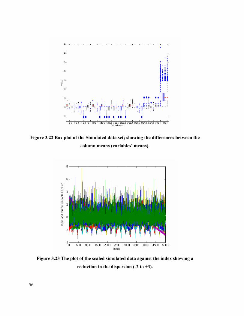
56

Figure 3.22 Box plot of the Simulated data set; showing the differences between the

column means (variables' means).

Figure 3.23 The plot of the scaled simulated data against the index showing a

reduction in the dispersion (-2 to +3).

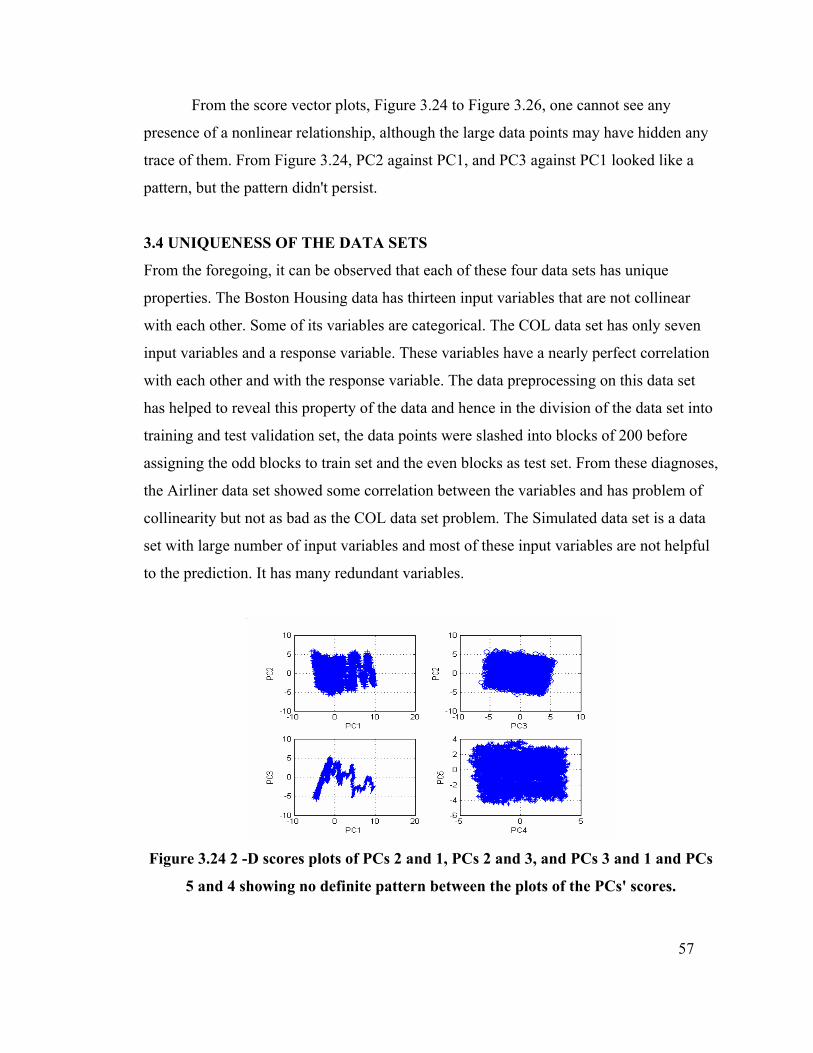
57

From the score vector plots, Figure 3.24 to Figure 3.26, one cannot see any

presence of a nonlinear relationship, although the large data points may have hidden any

trace of them. From Figure 3.24, PC2 against PC1, and PC3 against PC1 looked like a

pattern, but the pattern didn't persist.

3.4 UNIQUENESS OF THE DATA SETS

From the foregoing, it can be observed that each of these four data sets has unique

properties. The Boston Housing data has thirteen input variables that are not collinear

with each other. Some of its variables are categorical. The COL data set has only seven

input variables and a response variable. These variables have a nearly perfect correlation

with each other and with the response variable. The data preprocessing on this data set

has helped to reveal this property of the data and hence in the division of the data set into

training and test validation set, the data points were slashed into blocks of 200 before

assigning the odd blocks to train set and the even blocks as test set. From these diagnoses,

the Airliner data set showed some correlation between the variables and has problem of

collinearity but not as bad as the COL data set problem. The Simulated data set is a data

set with large number of input variables and most of these input variables are not helpful

to the prediction. It has many redundant variables.

Figure 3.24 2 -D scores plots of PCs 2 and 1, PCs 2 and 3, and PCs 3 and 1 and PCs

5 and 4 showing no definite pattern between the plots of the PCs' scores.

58

Figure 3.25 2-D scores plots of PCs 8 and 7, PCs 7 and 1, PCs 8 and 5, and PCs 8

and 9 showing no definite pattern between the plots of the PCs' scores.

Figure 3.26 2-D scores plots of PCs 9 and 1, 23 and 21, 18 and 12, 43 and 42 showing

no definite pattern between the plots of the PCs' scores.

59

4.0 RESULTS AND COMPARISON

In Chapter Three, the different data sets used in this study were introduced, preprocessed,

and analyzed to gain a superficial insight into their attributes. In this chapter, for each

data set, the various predictive data-mining techniques will be used to build models in

order to compare their predictive abilities with each other. The resulting predictions of

the output or response variables will be compared with the existing output variable, and

the differences will be measured using established statistics or statistical methods.

4.1 THE STATISTICS OR CRITERIA USED IN THE COMPARISON

In Chapter five, five criteria for model comparison were use. In this section, the entire

nine criteria used to compare the various methods within each technique are briefly

explained.

1. R-square (R2 or R-Sq) measures the percentage variability in the given data matrix

accounted for by the built model (values from 0 to 1).

2. R-square Adjusted (R2adj) gives a better estimation of the R2 because it is not

particularly affected by outliers. While R-sq increases when a feature (input variable)

is added, R2adj only increases if the added feature has additional information added to

the model. R2adj values ranged from 0 to 1.

3. Mean Square Error (MSE). MSE measures the difference between the predicted test

output and the actual test outputs. The smaller the MSE, the better. Large MSE values

mean poor prediction, as was explained in Section 2.6.2a.

4. Root Mean Square Error (RMSE); this is just the MSE in the units of the original

predicted data. It is calculated by finding the square root of MSE.

5. Mean Absolute Error (MAE); this quantity takes care of overestimation due to

outliers, as was discussed in Section 2.6.2e.

6. Modified Coefficient of Efficiency (E-mod); the modified coefficient of efficiency

gives information equivalent to the MAE (values from -1 to 1). See Section 2.6.2e.

60

7. The Weight of the regression models (norm); this value calculates the weights of the

regression coefficients. See Section 2.6.2b.

8. Condition number of the predictor matrix (CN); this quantity, designated as CN here,

gives a measure of the stability of the model built. High condition numbers (> 100)

show that the problem is ill-conditioned and hence cannot give consistent or stable

results. See Section 2.6.2b.

9. Number of features or variables used (N). The objective of every builder is to make

use of the smallest amount of resources to achieve the desired result, as per Occam's

Razor. Since data collection and analysis are expensive, fewer features (variables)

take less energy and resources to deal with. See Section 2.6.2c.

The data sets are divided into two: the training set and the test data sets (odd-

numbered data points are the training set and even-numbered data points are the test set).

The train set predictor (input) variables are used to build the model. The train set

predictor is regressed against the train response variable, and the resulting regression

constants are called the regression coefficients. These coefficients are post-multiplied

with the train set input variables to get the predicted train set response variable. This is

called the training. When the prediction is compared with (subtracted from) the original

train data, the difference between the prediction and the original output is revealed. When

the same coefficients are post-multiplied with the test set input (predictor) variables, the

result is also compared with the test set original response output. The test set is used to

confirm the soundness of the model. The ability to accurately predict the test output tells

how good the model is and is a measure of model performance.

The results from the predicted training sets' output are important because a model is

expected to perform well in the training set used to build the model. In this work

however, the results were not included because of size and most importantly, in real-life

analysis, the soundness of the model is only measured by its ability to predict new data

sets and not the train data sets from where the model was trained. If a model performed

very well in the training set and could not perform satisfactorily in the test validation data

set or new data sets, then its predictive ability is suspect and cannot be used for

61

prediction. Hence, the results of the predictions of the training sets' output were not

presented in this analysis because the performances of the models in the test validation

data set are of more significance to this study. Only the predictions of the response

variables of the test validation data sets were used for the model comparison.

4.2 BOSTON HOUSING DATA ANALYSIS

The Boston Housing data set has thirteen predictor variables and one response variable

(median value of the owner-occupied homes in $1000's, Mval) In this section, the five

predictive data mining techniques are used to predict the response variable (Mval).

4.2.1 Multiple Linear Regression (MLR) Models on Boston Housing Data

In the multiple linear regression (MLR), three methods are considered: full model

regression, stepwise regression, and selection of variables based on their correlation with

the response variable using the correlation coefficient matrix of all the variables.

a. Full model regression, (all thirteen variables). The full model used all the response

variables to predict the output Yi.

01

k

i j ij ij

y kβ β ε=

= + +∑ where i =1, 2, 3, …14.

It gives a result of thirteen regression coefficients βj: thirteen constants representing

the slope of the regression line (β2 to β14) and one constant (β0) representing the intercept

on the Y- axis if a column of ones is appended to the data matrix before regressing. The

different between the prediction and the predicted is given as Yi – Y = εi. The results are

summarized in Table 4.1 for the full model. The condition number of the regression

model is 7.33 e+7. This is very large and shows the model to be highly ill-conditioned.

Therefore, the solution will be very unstable and unrealistic. Little perturbation on the

input variables will result in a large change in the output. The norms (weights) of the

regression coefficients are also large. This is further evidence of the instability of the

model. From the calculated adjusted R-squared, 73% of the variation in the data is

accounted for by the model.

62

Table 4.1 Summary of the results of the three MLR models. MLR R-Sq R-sq-

Adj

MSE RMSE MAE E-mod. CN Norm

Wt.

N

Full model 0.7445 0.7306 21.1503 4.5989 3.2500 0.4405 7.33e+7 43.1679 13

Cor.Coeff. 0.7038 0.6915 24.5201 4.9518 3.4430 0.3645 7.14e+7 5.6481 11

Stepwise 0.6727 0.6968 24.5971 4.9595 3.3989 0.3809 2.122+7 9.0145 6

b. Correlation based model. The correlation coefficient matrix is used to choose

variables that are best correlated with the output variables.

The correlation coefficient matrix of all the input variables with the output variable is

shown in the Appendix A, Table A.1. The column of interest is the 14th column. This

column has the correlation coefficients of all the other 13 variables with the output

variable. Only coefficients with absolute value => 3 will go into the model. All the

correlated variables were used to build the regression model: Variables 1 to 3, 5 to 7, and

9 to 13 (CRIM, ZN, INDUS, NOX, RM, AGE, RAD, TAX, P/T ratio, Black, and %

lower Stat (see Section 3.2.1)). The result of the correlation-built model is shown in the

Summary Table 4.1.

c. Stepwise Regression. The stepwise regression model built with MATLAB only gives

results of the training data set prediction. Variables that are significantly different

from zero made the model, and the same variables were used to build a multiple

linear regression.

From Figure 4.1, the train data set prediction gave RMSE of 5.115 (MSE = 26.163) and

R-square value of 0.7044. Figure 4.2 shows the eliminated variables in the model in

broken lines and touching the center line. From the inbuilt stepwise regression tool in

MATLAB, only Variables 5, 6, 8, 11, 12, 13 (NOX, RM, DIS, P/T ratio, Black, LStat. )

were statistically significant enough to be in the model. Seventy percent of the variability

in the training data set was explained by the model. This is very close to the R-square in

the full model (see Table 4.1). The six variables used in building the regression model do

not have their confidence interval lines (solid) crossing or touching the zero line (Figure

4.2).

63

Confidence IntervalsColumn #

RMSE

Parameter

R-square

Lower

F

Upper

P


RMSE

Parameter

R-square

Lower

F

Upper

P


RMSE

Parameter

R-square

Lower

F

Upper

P


RMSE

Parameter

R-square

Lower

F

Upper

P


RMSE

Parameter

R-square

Lower

F

Upper

P


RMSE

Parameter

R-square

Lower

F

Upper

P


RMSE

Parameter

R-square

Lower

F

Upper

P


RMSE

Parameter

R-square

Lower

F

Upper

P


RMSE

Parameter

R-square

Lower

F

Upper

P

1 -0.5018 -1.61 0.6064 2 0.803 -0.5298 2.136 3 -0.5729 -2.237 1.091 4 0.694 -0.282 1.67 5 -2.112 -3.729 -0.4953 6 2.932 1.62 4.243 7 -0.4832 -2.11 1.144 8 -2.704 -4.218 -1.19 9 0.8451 -0.5449 2.235

10 0.02111 -1.432 1.474 11 -2.149 -3.189 -1.11 12 1.037 0.004212 2.07 13 -3.834 -5.339 -2.328

5.115 0.7044 97.68 0

Figure 4.1Confidence interval and parameter estimation using Stepwise regression

(MATLAB output) Boston Housing data.

-4 -2 0 2 4

1

2

3

4

5

6

7

8

9

10

11

12

13

Coefficients with Error Bars

Mod

el T

erm

Num

ber

Figure 4.2 Confidence Interval lines for the training data set prediction (MATLAB

output) for the Boston Housing data.

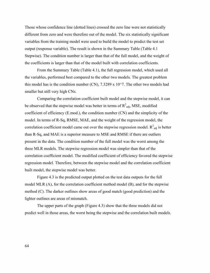
64

Those whose confidence line (dotted lines) crossed the zero line were not statistically

different from zero and were therefore out of the model. The six statistically significant

variables from the training model were used to build the model to predict the test set

output (response variable). The result is shown in the Summary Table (Table 4.1

Stepwise). The condition number is larger than that of the full model, and the weight of

the coefficients is larger than that of the model built with correlation coefficients.

From the Summary Table (Table 4.1), the full regression model, which used all

the variables, performed best compared to the other two models. The greatest problem

this model has is the condition number (CN), 7.3289 x 10^7. The other two models had

smaller but still very high CNs.

Comparing the correlation coefficient built model and the stepwise model, it can

be observed that the stepwise model was better in terms of R2adj, MSE, modified

coefficient of efficiency (E.mod.), the condition number (CN) and the simplicity of the

model. In terms of R-Sq, RMSE, MAE, and the weight of the regression model, the

correlation coefficient model came out over the stepwise regression model. R2adj is better

than R-Sq, and MAE is a superior measure to MSE and RMSE if there are outliers

present in the data. The condition number of the full model was the worst among the

three MLR models. The stepwise regression model was simpler than that of the

correlation coefficient model. The modified coefficient of efficiency favored the stepwise

regression model. Therefore, between the stepwise model and the correlation coefficient

built model, the stepwise model was better.

Figure 4.3 is the predicted output plotted on the test data outputs for the full

model MLR (A), for the correlation coefficient method model (B), and for the stepwise

method (C). The darker outlines show areas of good match (good prediction) and the

lighter outlines are areas of mismatch.

The upper parts of the graph (Figure 4.3) show that the three models did not

predict well in those areas, the worst being the stepwise and the correlation built models.

65

Figure 4.3 The model-predicted output on the test data outputs for the Boston

Housing data.

4.2.2 Principal Component Regression (PCR) on Boston Housing Data

For the principal component regression, the train data set was scaled (standardized) and

the means and standard deviations of the columns of this scaled training set were used to

scale the test data set. Here, different methods of selecting the significant PCs are used.

The reduced singular value decomposition (SVD) of the scaled data sets and the resultant

Eigen vectors and singular values reveals the variables that played dominant roles (called

the heavy weights) in each principal component (PC). The condition number of the

standardized data was now 87.5639. This is a large reduction from the 7.3289e+7 of the

original raw data matrix.

The PC loadings show the weights of each variable in the different PCs. Variables

9 and 10 (Accessibility to highway and Full-value property-tax rate) are the least

significant variables in the group. They are the dominant variables in the least significant

PC (13th PC). Figures 4.4 and 4.5 show the first thirteen principal component loadings. In

Figure 4.4, the first principal component (carrying 22.6% information), Variables 3

(INDUS), 5 (NOX), 10 (TAX), 8 (DIS), 9 (RAD), 7 (AGE), and 13 (LSTAT) in that

order came out stronger than 1, 2, 4, 6, 11, or 12. The heaviest was Variable 3 and the

least was Variable 4. In the second PC with 11% information, Variable 4 (CHAS) was

the dominant variable (heavy weight). The third PC with 10% information had Variable 6

(RM) as the heavy weight.

66

Figure 4.4 PC Loadings showing the dominant variables in the PCs 1 to 6.

Figure 4.5 Loadings for the 7th to 13th principal components showing the dominant

variables in those PCs.

67

The fourth PC with 8.4% information had Variable 11 as its dominant variable; the

fifth PC (8.3%), Variable 4 (CHAS); the sixth PC (7.5%), variable 12 (Black); the

seventh PC (6.9% information), Variable 1 (CRIME); the eighth PC (5.6% information),

Variable 7 (AGE); the ninth PC (5% information), Variable 3 (INDUS); the tenth PC (4%

information), Variable 13 (LSTAT); the eleventh PC (3.99%), Variable 8 (DIS); the

twelfth PC (3.7% information), Variable 5 (NOX); and the thirteenth PC (carrying 2.4%

information) had variable 10 (TAX) s the heavy weight. The numbering of the PCs

differs from that of the variables. If we choose PC 1, it should be noted that the variables

playing strongly in PC 1 become the choice for the model, with the heaviest variable in

that PC leading the pack.

To choose the most significant PCs, which were used to build the model (Section

2.3.2), a scree plot of the eigenvalues against the PCs was made (Figure 4.6). This is built

from Table 4.2. The percentage explained was plotted against the number of PCs. This

plot helped in the selection of the number of significant PCs, looking out for points of

major "knees," which are points of significant change in the difference in the singular

values.

a. The first model was built with all the principal components (PCR Full model).

This used all the 13 PCs in the pack, similar to using all the 13 variables in the MLR

Section 4.2), but with the data set standardized.

b. From the scree plot, Figure 4.6, the first major "knee" was at the 4th PC. PCs 1 to 4

explained 52.477% of the variation in the data.

c. Another major point of inflection was at PC 10. This second "knee" carried 89.85%

of the information of all the information of the whole data matrix.

d. The model was built from the PCs having up to 90% of the explained information in

the data matrix. This included PC 11 and covered the significant PCs when all the

singular values less than 1 were dropped.

68

Table 4.2 Table showing the Percentage of Explained Information and the

Cumulative Explained information. PCs % Explained Cumulative of % Explained

1 22.5740 22.5740

2 11.3324 33.9064

3 10.1320 44.0384

4 8.4386 52.4770

5 8.2767 60.7537

6 7.4787 68.2324

7 6.8960 75.1285

8 5.5824 80.7109

9 5.0032 85.7141

10 4.1386 89.8527

11 3.9928 93.8455

12 3.7421 97.5876

13 2.4124 100.0000

0 2 4 6 8 10 12 140

5

10

15

20

25

30

35

40

Number of PCs

Eig

enva

lues

Figure 4.6 Scree plot of the Eigenvalues vs. the PCs.

69

e. The fifth PCR model was built using the highest correlated score of the PCs with the

response variable. Table 4.3 shows only the 14th column of this matrix. In this case,

the rule of coefficients equal to or greater than the absolute value of 0.3 was not

applied since most of the coefficients were less than that. The first 3 PCs had

reasonable correlation with the response variable. PC 4, 5 and 12 looked somewhat

strong in relation to the others.

The summary of the results of the PCR built models are given in Table 4.4. It can

be observed that there is controversy over which model is better, between the model with

11 PCs (=>90% variation) and that built with 10 PCs. Using the MSE, RMSE, R2adj., the

condition number (CN), the weight of the regression coefficients (Norm) and considering

the simplicity of the model, the model with ten PCs came out over that with eleven PCs.

Using MAE and modified coefficient of efficiency, however, the model built

with eleven PCs looked better. Thus, of those two options, the model with ten PCs will

rule over that with eleven PCs.

Table 4.3 The 14th column of the correlation coefficient matrix of the Boston housing

data set. PCs Output

1 -0.6036

2 0.3543

3 0.3872

4 0.1604

5 -0.1212

6 -0.0800

7 -0.0126

8 -0.0633

9 0.0069

10 -0.0190

11 -0.0837

12 0.1597

13 -0.0818

Output 1.0000

70

Table 4.4 Summary of the Results from All the Methods of Principal Component

Regression Models. PCR R-Sq R-sq-

Adj


Wt.

# of

PCs

Full 0.7445 0.7317 21.1503 4.5989 3.250 0.4405 87.5639 0.7893 13

=>90% 0.7160 0.7043 23.5042 4.8481 3.3517 0.3948 31.9635 0.6108 11

2nd Knee 0.7181 0.7077 23.3328 4.8304 3.3714 0.3833 29.7520 0.5798 10

1st Knee 0.6943 0.6906 25.3053 5.0304 3.4919 0.3432 7.1561 0.5435 4

Cor.PCs (1-3) 0.6716 0.6690 27.1818 5.2136 3.5908 0.3393 7.1561 0.5148 3

Cor. PCs

(1-5,12)

0.7280 0.7225 22.5133 4.7448 3.3975 0.3919 36.3902 0.6831 6

A look at the last two models built from the correlated PCs will reveal that they

looked more reasonable than any other because those were the PCs having the best

correlation with the response variable. The variables that were dominant variables in

these PCs (1-5 and 12), were 3, 5, 10, 8, 9, 7, 13 (all from the first PC), 4 (from the

second PC), 6 (from the third PC), 11 (from the fourth PC), 4 again (from the fifth PC)

and 5 again (from the twelfth PC). Considering the weights and the simplicity of model,

the first correlation model (with 3 PCs) ranked better than all the other PCs.

In terms of R-Sq, R2adj, modified coefficient of efficiency, RMSE and MAE, the

first correlation-based model (with three variables) looked almost the same as the model

with 4 PCs. Their condition numbers were the same. With the second correlation model,

only the full model (all PCs) outperformed it in terms of the first six criteria (see the

Summary Table 4.4).

In terms of the weight, condition number and simplicity of the model, the second

correlation model (with 6 PCs) was better. It gave more consistent, stable results with less

computing expense. The Full model of the PCR, therefore, is the best model for the

Boston Housing data.

Figure 4.7 shows the plot of the prediction over the outputs of the test data. The

prediction came out as the darker outline in the graph, and the faint-colored areas were

points of mismatch. There were mismatches especially at the upper parts of the test

71

Figure 4.7 The predicted output upon the Test Data Outputs for the Best Two PCR

models.

output. Those may also be outliers which were not captured by the model. Toward the

last quarter of the graph (from data points 200 to 250), the full model in Figure 4.7 (lower

plot) did better than all others.

The plots showing the predicted outputs upon the test data outputs for the PCR

models with 10 PCs, 11 PCs, 4 PCs, and the first correlation-based model (3 PCs) are

shown in Appendix B, Figure B.1 and Figure B.2.

4.2.3 Ridge Regression on Boston Housing Data

Five ridge regression models were built out of two well known methods (ordinary ridge

regression and ridge regression using an L-Curve).

a. The ordinary ridge model was built without standardizing the data sets and having a

zero alpha.

b. The ridge model was built using L-Curve with the data set not standardized.

c. The ordinary ridge model was built with data standardized with zero alpha. This is the

same as the full model PCR.

d. Ridge regression was built using regularization coefficients 'alpha' (α).

72

Figure 4.8 Plot of the MSE vs. Alpha for Ridge regression on the Boston Housing

data.

In the literature, the optimal alpha value is slightly less than the least significant

singular value [54]. To get the optimal alpha, the whole range of the singular values is

used, and the alpha value that strikes a good compromise between the condition number,

the weight of the regression coefficients, and the mean square error is selected for the

model. That alpha value should be slightly less than the least significant singular values.

Table 4.5 shows the singular values of the Boston Housing data. The whole range of the

singular values is used iteratively as alpha values, and the optimal alpha value is that

which satisfies the compromise mentioned earlier. The singular values ranged from 4 to

40 (Table 4.5), so alpha values in this range were used.

The resulting mean square errors from the iterations were recorded and plotted

against the alpha values. This plot (Figure 4.8), of MSE vs. Alpha, gives the minimum

MSE obtainable from ridge regression. The alpha value increases with an increase in the

MSE. The condition number at such a minimum MSE can also be computed from the

iteration results. The relationship between alpha and the condition number is shown in

Figure 4.9. The alpha is negatively related with the condition number (the condition

number increases with a decrease in the alpha value). The goal is to get a model with the

least MSE and a relatively low condition number.

73

Table 4.5 Singular Values (SV) for the Boston housing data. PCs SV

1 39.0822

2 19.6197

3 17.5415

4 14.6097

5 14.3294

6 12.9478

7 11.9390

8 9.6648

9 8.6621

10 7.1651

11 6.9128

12 6.4787

13 4.1765

Figure 4.9 Plot of the Regularization Coefficient vs. the Condition Number for

Ridge regression on the Boston Housing data.

74

The weight of the regression coefficients, which is positively related to the condition

number, has the same negative relationship with alpha as the condition number. This is

shown in Figure 4.10. The norm vs. MSE graph in Figure 4.11 was used to find the

optimal alpha value corresponding to the minimum MSE that satisfied this compromise

between the MSE and the condition number. This is called the L-Curve. This gives the

best trade-off between the smoothing parameter and the bias.

From Figure 4.11, the point on the norm axes corresponding to the minimum

MSE were marked (0.75) and a point a little below it was chosen (between 0.6 and 0.7 on

the norm axes). This point gave a better (optimal) alpha value in that it took care of the

trade-off between the smoothing and the minimum error. As the weight was decreased,

smoothing was taking place (alpha was increasing) and at the same time, the MSE was

increasing. The weight or norm of 0.65 gave a corresponding MSE value of 21.6261. The

corresponding alpha (optimal) value is 4.0949. This is slightly less than the last singular

value (and the least significant singular value) in Table 4.5. A point on the norm axes,

0.8, gives the corresponding minimum MSE obtainable from ridge regression (MSE =

21.1576).

Figure 4.10 Plot of the Weight vs. the Regularization Coefficient (alpha) for Ridge

regression on the Boston Housing data.

75

Figure 4.11 Norm vs. MSE (L-Curve) for Ridge regression on the Boston Housing

data.

From the Summary, Table 4.6, showing the ridge regression results, the best

models were those built from standardized data (the last three shown in Table 4.6).

Among these, the best solution came from the model built with a regularization parameter

(optimal alpha value) of 4.0949. It gave a very stable result with comparatively good

MSE, good modified coefficient of efficiency and a good condition number. The model

with alpha value of 1 was also good but the stability of the result compared to that of

alpha value of 4.0949 was not very good.

Using the L-Curve on the raw data gave very bad results. The alpha value used

was not even within the range of the alpha values in Table 4.5, perhaps because the

singular values were computed from the scaled data. The MSE values from the raw data

models were very high compared to others.

Figure 4.12 (A) shows a total mismatch between the prediction and the output in

model built with raw data in ordinary ridge regression. Ridge regression should be used

with data standardized. B was the result from using an alpha value of zero but with

standardized data.

76

Table 4.6 Summary of the Ridge Regression Results on Boston Housing data. RIDGE R-Sq R-sq-

Adj


Wt.

N

Raw Data 0.000 0.0000 340100 580 460 0.000 7.3 e+7 23.6106 13

Raw data α = 72 4414.7 66.4432 2331.6 1.1991 13

Scaled data α=0 0.7160 0.7043 23.5042 4.8481 3.3517 0.3948 31.9635 0.6108 13

Scaled data,α=1 0.7444 0.7305 21.1576 4.5997 3.2429 0.4396 82.8704 1 13

Scaled data, α =

4.0949

0.7387 0.7257 21.6261 4.6504 3.2255 0.4166 45.1361 0.6534 13

0 50 100 150 200 250 300-1500

-1000

-500

0

500

A. Observations for the Unstandardized data, mse = 340100

Am

plitu

de

Test OutputPrediction

0 50 100 150 200 250 3000

10

20

30

40

50

C. Observations for the model with 4.0949 optimal alpha value and mse = 23.5042

Am

plitu

de

Test OutputPrediction

Figure 4.12 Predicted Output over the Original Output of the test data.

77

4.2.4 Partial Least Squares (PLS) on Boston Housing Data

The condition numbers of the PLS models were the same with those of the PCR with

corresponding number of PCs or factors because the data set was standardized and both

used factors or PCs. Also, as the number of factors used was less than the total number of

factors, the condition numbers continued to improve.

To get the minimal eigenfactor in order to build the PLS model, Malinowski's

reduced eigenvalues were computed and plotted against the index (Figure 4.13). From

Figure 4.13, only two factors or three seemed to be good enough to build the model using

the PLS technique. From Table A.5 in the Appendix, the result of the reduced

eigenvalues became basically equal from factor 6, so one can conclude that factors 6 to

13 accounted for noise; hence, the first five factors were also good for building the

model.

The optimal number of factors was found by using the iterative method to get the

least MSE using all the factors. Table 4.7 shows the result of this generalization method.

Iteratively using all the factors and plotting the resulting mean square errors against the

latent factors showed that the factor that gave the least MSE was the optimal factor (see

Figure 4.14).

Figure 4.13 A plot of the reduced eigenvalues vs. Index.

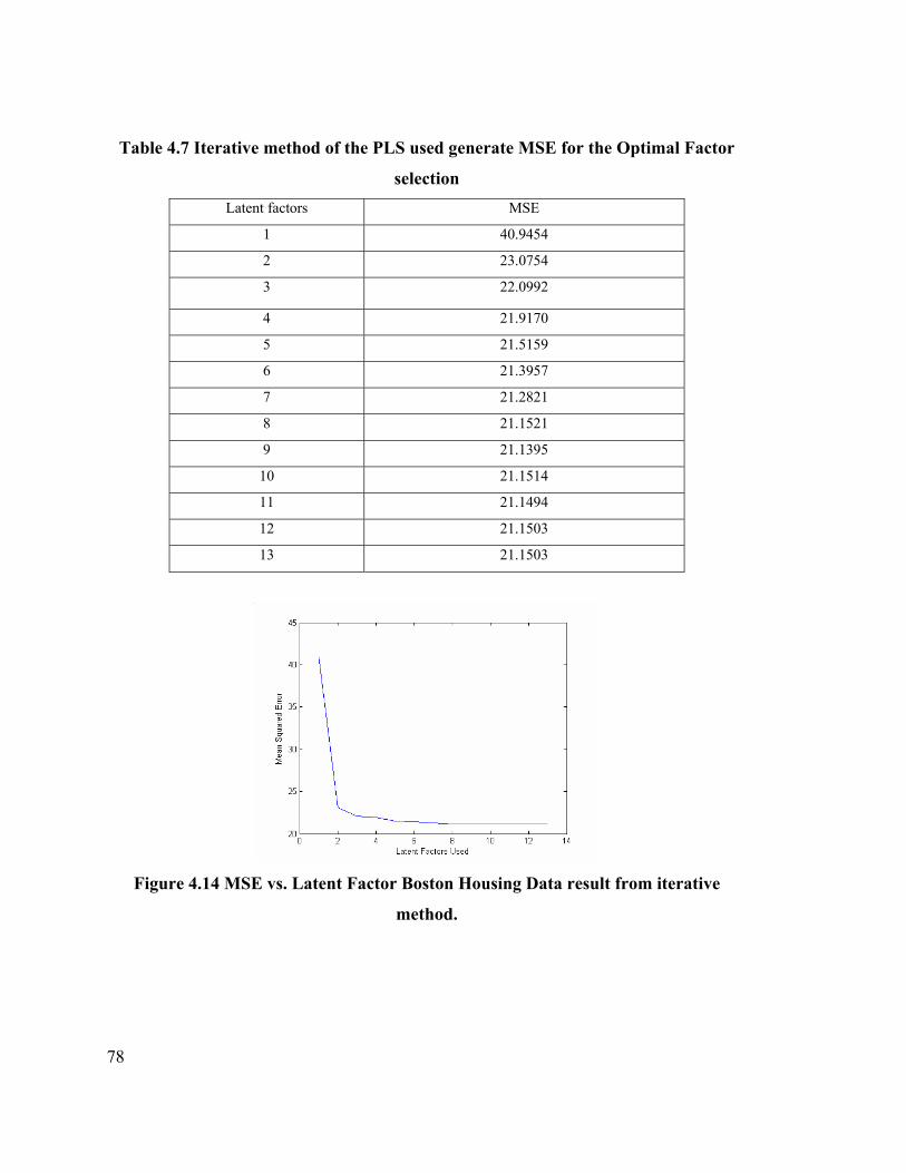
78

Table 4.7 Iterative method of the PLS used generate MSE for the Optimal Factor

selection Latent factors MSE

1 40.9454

2 23.0754

3 22.0992

4 21.9170

5 21.5159

6 21.3957

7 21.2821

8 21.1521

9 21.1395

10 21.1514

11 21.1494

12 21.1503

13 21.1503

Figure 4.14 MSE vs. Latent Factor Boston Housing Data result from iterative

method.

79

The minimum MSE was at the ninth factor and the value was 21.1395. Finally, all

thirteen factors could be used to build a model to compare with the other models.

From the Summary Table 4.8, it can be observed that the model with nine factors

outperformed every other model in PLS. The model with all the factors (thirteen factors)

was better only with R2adj and performed the same as the model with nine factors in terms

of RMSE. In terms of every other criterion except MAE, the model with nine factors

performed better. The best model in terms of MAE was the model with three factors and

its condition number was very good at 7.2.

Figure 4.15 (A) is the plot of the prediction on the original output data for nine

factors and (B) is the prediction on the original output built with all the thirteen factors.

There were many outliers in this data set. The model could not predict well in the range

of data values, 40 to 50. Hence, the upper parts of the plot are faint because the prediction

did not cover that area.

Figure 4.16 shows the output scores “U” plotted over the input scores “T.” The

prediction is the straight line. This shows the output scores plotted upon the input scores

from the various factors. It can be observed that the model has a strong linear

relationship. Figure 4.16 A shows the presence of nonlinearity in the data. This is seen at

the upper part of the first and second plots in Figure 4.16. Perhaps with Nonlinear Partial

Least Squares, the nonlinearity may be mapped into the mode.

Table 4.8 Summary of Results Using PLS Regression on Boston Housing Data. PLS R-Sq R-sq-

Adj


Wt.

# of

Factors

Red.eig 1 0.7212 0.7201 23.0754 4.8037 3.3019 0.3952 <7 <0.5 2

Red.eig 2 0.7330 0.7309 22.0992 4.7010 3.2433 0.4204 7.2 0.5148 3

Min.eig. 0.7400 0.7359 21.5159 4.6385 3.2928 0.4360 <36 <0.683 5

Optimal 0.7446 0.7307 21.1395 4.5978 3.2498 0.4408 <29 0.5798 9

All factors 0.7445 0.7317 21.1503 4.5978 3.2500 0.4405 87.5639 0.7893 13

80

Figure 4.15 The predicted plotted upon the original output for nine eigen factors (A)

and all the eigen factors (B) for the Boston Housing Data.

Figure 4.16 Output scores 'U' plotted over the input scores 'T' (predicted and test

response).

81

4.2.5 Nonlinear Partial Least Squares (NLPLS) on Boston Housing Data

Using the training function in the neural network toolbox, the training data set was

trained as many times as the number of variables in the matrix. The NLPLS function

performed iterative computation to find the minimum mean absolute error (MAE). This

was plotted against the latent factors (Figure 4.17) and the point inflection, a global

minimum, was noted (minimum MAE and optimal number of factors).

The optimal number of latent factors was found by finding the corresponding

minimum Mean Absolute Error (2.954465). This optimal number of latent factors was 4

(see Figure 4.17) in this case.

The result of the NLPLS is shown in Table 4.9. All the measured parameters are

better in the NLPLS. It is possible that NLPLS mapped also nonlinearity into the model.

Figure 4.17 Plot of the Mean Absolute Error vs. latent factors showing 4 optimal

latent factors.

Table 4.9 Result of the Non-linear Partial Least Squares on Boston Housing Data. NLPLS R-Sq R-sq-Adj MSE RMSE MAE E-mod. CN Norm factors

1st 0.7831 0.7805 17.9547 4.2373 2.9545 0.5121 4

2nd 0.7921 0.7853 17.9547 4.1478 2.9120 0.5180 9

3rd 0.7925 0.7866 17.1734 4.1441 2.9182 0.5216 8

82

The MSE was 17.9547, which was the least among all the models. The NLPLS

prediction results seem to be better than the rest, but some nonlinearity was mapped into

the model. Figure 4.19 shows that the Nonlinear Partial Least Squares mapped most of

the information in the data matrix; there are signs of nonlinearity in the predictions,

though not strong. In Chapter 5, we shall do a final comparison of the various techniques

on each data set comparing the best from each technique.

Figure 4.18 shows the prediction using NLPLS. Points of mismatch were small

compared to the other models. From this graph, it can be observed the NLPLS mapped

those areas that PLS could not map. NLPLS models over-fit the model and included

noise or nonlinear information contained in the data.

Figure 4.18 NLPLS prediction of the test output using four factors for the Boston

Housing data.

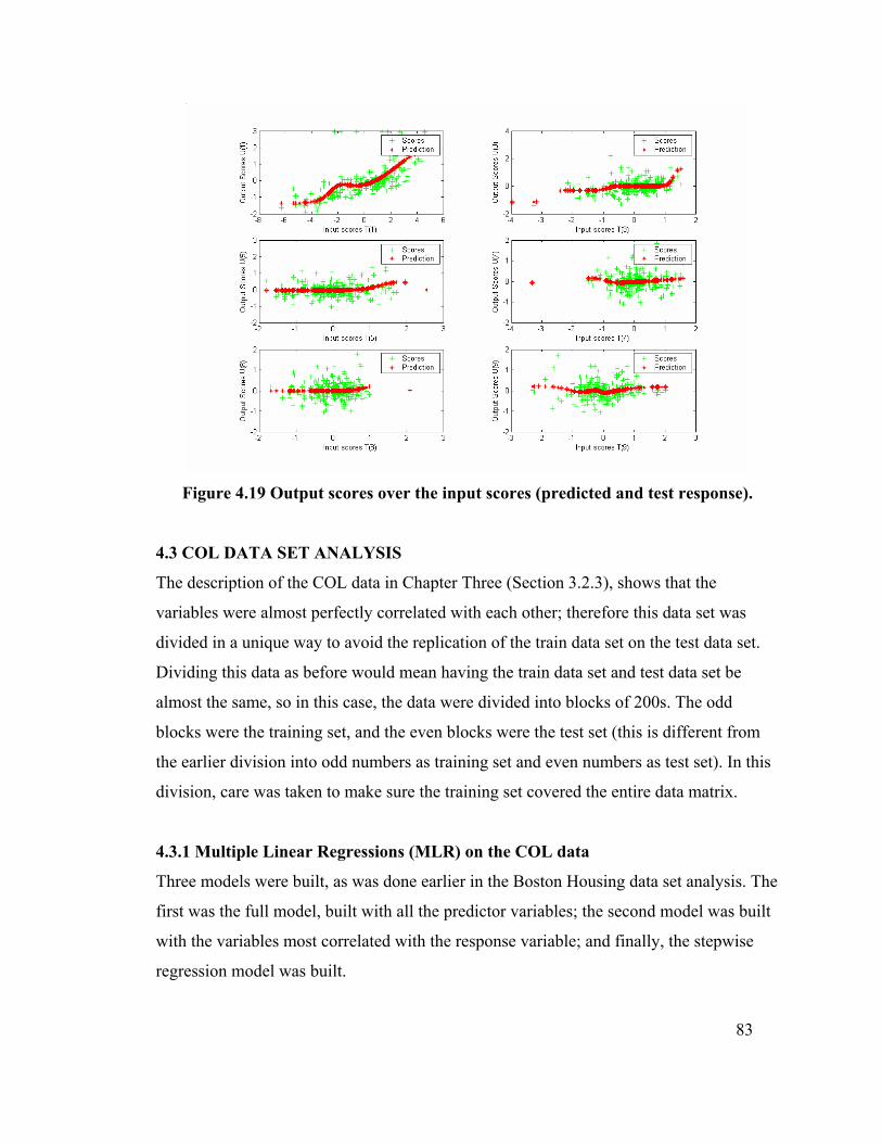
83

Figure 4.19 Output scores over the input scores (predicted and test response).

4.3 COL DATA SET ANALYSIS

The description of the COL data in Chapter Three (Section 3.2.3), shows that the

variables were almost perfectly correlated with each other; therefore this data set was

divided in a unique way to avoid the replication of the train data set on the test data set.

Dividing this data as before would mean having the train data set and test data set be

almost the same, so in this case, the data were divided into blocks of 200s. The odd

blocks were the training set, and the even blocks were the test set (this is different from

the earlier division into odd numbers as training set and even numbers as test set). In this

division, care was taken to make sure the training set covered the entire data matrix.

4.3.1 Multiple Linear Regressions (MLR) on the COL data

Three models were built, as was done earlier in the Boston Housing data set analysis. The

first was the full model, built with all the predictor variables; the second model was built

with the variables most correlated with the response variable; and finally, the stepwise

regression model was built.

84

a. The full model was built with all the seven input variables in the COL data.

b. The correlation coefficient-built model was built using only the variables that most

correlated with the output variables. The whole correlation coefficient matrix of the

COL data is shown in Appendix Figure A.2. The column of interest here is the eighth

column, shown in Table 4.10. From the figure in the Appendix (Figure A.2), all the

variables were almost perfectly correlated with each other. They may be carrying the

same information. All the variables were used in building the model, just as in the full

model.

c. Stepwise Method: As in the Boston Housing data analysis, the train set was used in

the stepwise method and the variables that gave the optimal result were used in the

validation test. Figures 4.20 and 4.21 show the MATLAB output for the training set.

Since all the variables are significantly different from zero, they were all used to build

this model. This gave the same result as in the full model (a) and correlated model (b).

Table 4.11 gives the result of the MLR on the COL data. It shows that all the

methods gave the same result. For a nearly perfectly correlated data set, the use of

stepwise or correlated variables does not make much difference. Figure 4.22 shows that

the prediction looks perfect, but that there is a serious problem of collinearity. The

condition number is too high, and this will make the model very unstable.

4.3.2 Principal Component Regression (PCR) on the COL data

From the loadings (Figure 4.23), the first PC carried most of the information (76%) in the

entire COL data matrix. It had all the variables as heavy weight. The second PC (11%

information) had only Variable 7 as the heavy weight. The third PC (6% information) had

Variables 7 and 1 as the heavy weights. The fourth and fifth PCs (3.3% and 1.7%

information respectively) had Variable 4 as the heaviest weight. The sixth PC (1.44%

information) had Variable 5 as the dominant variable, and the seventh PC carrying less

than 1% information, had Variable 5 as its dominant variable also.

85

Table 4.10 The correlation coefficient matrix of the scores with output (8th

column).

Output

1 0.8841

2 0.9038

3 0.9012

4 0.9249

5 0.8943

6 0.9935

7 0.9101

Output 1


RMSE

Parameter

R-square

Lower

F

Upper

P


RMSE

Parameter

R-square

Lower

F

Upper

P

1 -9.772 -11.9 -7.648 2 -39.64 -45.66 -33.62 3 16.62 11.82 21.41 4 53.78 51.16 56.41 5 -28.04 -31.84 -24.25 6 76.59 75.93 77.25 7 10.33 8.057 12.61

5.356 0.9956 1.576e+005 0

Figure 4.20 Results of the training set used in building the model (MSE = 28.6867).

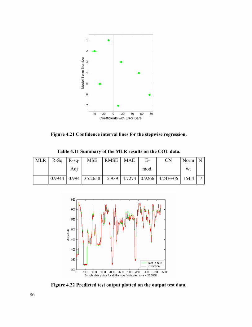
86

-40 -20 0 20 40 60 80

1

2

3

4

5

6

7


Mod

el T

erm

Num

ber

Figure 4.21 Confidence interval lines for the stepwise regression.

Table 4.11 Summary of the MLR results on the COL data.

MLR R-Sq R-sq-

Adj

MSE RMSE MAE E-

mod.

CN Norm

wt

N

0.9944 0.994 35.2658 5.939 4.7274 0.9266 4.24E+06 164.4 7

Figure 4.22 Predicted test output plotted on the output test data.

87

Figure 4.23 Loadings of the seven PCs showing the dominant variables in each

principal component.

Table 4.12 is the computed percentage of Explained Information and the

cumulative of the percentage of Explained Information. This was used to plot the scree

plot in Figure 4.24. This graph was used to select the number of PC to build the model.

a. The knee in the graph is at the second PC (see the scree Figure 4.24 )

b. The second model will be built with PCs that made up to 90% variation

(information) in the data. This comprised of the first three PCs.

c. The third model will be built with the scores that have higher correlation

coefficient with the output variable. Only the first two have considerable

correlation coefficients with the output variable. Table 4.13 is the 13th column of

this correlation coefficient matrix.

d. Model without the PC with less than 1% Information Explained. This gives six

PCs for the model leaving out the last PC.

e. The full model is built with all the seven PCs. This is equivalent to using the

whole input variables but standardized.

88

From the Summary Table (Table 4.14), with the MSE, the full model outperformed other

models but the full model had a serious problem of a very high condition number. The

model is therefore very unstable. The model that gave the best results with reasonable

consistency was the correlation-based built model. The condition number was below 100

but the MSE was high compared to the full model. It is a very simple model and has high

R2adj and modified coefficient of efficiency. The model built with variables whose scores

were correlated with the output was the best in PCR on the COL data. Even with fewer

PCs, it outperformed the model built with three PCs. Figure 4.25 is the PCR prediction on

the output data. Figure 4.25 (A) is the prediction using the first two PCs or correlated

PCs, (B) with the first three PCs, (C) using all the PCs, and (D) using six PCs. Points of

matches can be seen at data points 500 and 2000 of the Figure 4.25 A and B.

Table 4.12 Percentage explained information and the cumulative explained

information. PCs Variables % Explain Cumulative % Explain

1 All seven 75.7972 75.7972

2 6 10.8138 86.6110

3 1, 7 6.1038 92.7148

4 1, 4, 7 3.3358 96.0506

5 1, 3, 4, 7 1.7069 97.7574

6 3, 5 1.4409 99.1984

7 2, 3 0.8016 100.0000

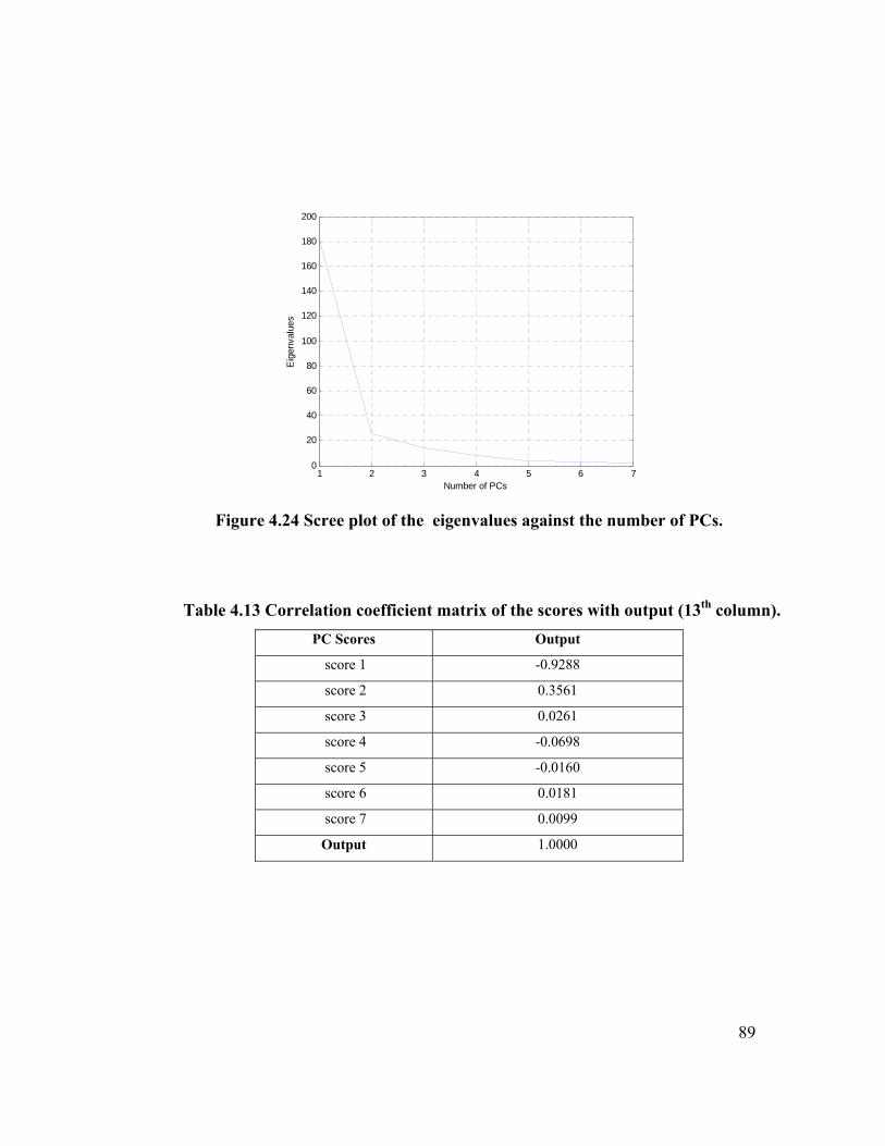
89

1 2 3 4 5 6 70

20

40

60

80

100

120

140

160

180

200

Number of PCs

Eig

enva

lues

Figure 4.24 Scree plot of the eigenvalues against the number of PCs.

Table 4.13 Correlation coefficient matrix of the scores with output (13th column). PC Scores Output

score 1 -0.9288

score 2 0.3561

score 3 0.0261

score 4 -0.0698

score 5 -0.0160

score 6 0.0181

score 7 0.0099

Output 1.0000

90

Table 4.14 Summary of the PCR Results on the COL Data.

PCR R-Sq R-sq-Adj MSE RMSE MAE E-mod. CN Norm PCs.

Knee 0.9899 0.9899 63.5893 7.9743 6.1286 0.9053 49.1301 1.0215 2

=>90% 0.9898 0.9898 64.4823 8.0301 6.152 0.9053 2311.4 1.029 3

Cor.built 0.9899 0.9899 63.5893 7.9743 6.1286 0.9053 49.1301 1.0215 2

<1% out 0.9942 0.9942 36.6783 6.0563 4.7118 0.927 2767.1 1.2796 6

All 0.9944 0.9944 35.2658 5.9385 4.7274 0.9266 8940.5 1.3288 7

Figure 4.25 PCR predictions on the output data.

91

4.3.3 Ridge Regression on the COL Data

Several methods were used to build ridge regression for the COL data:

a. Ordinary ridge regression with raw data (unstandardized data) with no regularization

parameter.

b. Ridge regression with raw data but using the L-curve;

c. Ordinary ridge regression with standardized data and zero regularization parameter;

d. Ridge regression model with standardized data and a regularization parameter α of

3.06 using the MSE-Alpha plot.

e. Ridge regression model with standardized data and a regularization parameter α of

13.3839 using the L-curve.

Table 4.15 shows the singular values of the data ranging between 1 and 182. The

alpha value can never be below 1 or above 182. To get the optimal alpha value, the

iterative method of regressing with all the ranges of the singular values was applied and

the resulting MSEs were plotted against the alpha values.

From the plot of MSE vs. alpha, Figure 4.26, the minimum MSE was 33.0767 and the

corresponding alpha value was 3.0888 and the condition number at this alpha value

Table 4.15 Singular Values (SV) of the COL data.

PCs SV

1 181.4238

2 25.8834

3 14.6096

4 7.9844

5 4.0854

6 3.4489

7 1.9187

92

was 1.49e+03. This solution is very biased, unsmooth, and unstable because of the high

condition number. We have already proved from the previous data set that the condition

number is negatively related with the regularization parameter, just as are the weights of

the regression coefficients in Figure 4.27. Using the plot of MSE and the weight or norm,

(L-curve; Figure 4.28), the best or optimal alpha value will be calculated.

A look at table 4.16 reveals that the ridge regression with the optimal alpha value

of 9 stands out in the ridge model. This is because it took care of the very high condition

number. The data set is highly collinear and hence is very ill-conditioned. Only an alpha

value that will make a compromise with MSE while smoothing will give a fairly

consistent and stable result. With an alpha value of 3.6, the solution seemed good, but the

condition number was still very high (1965.6); hence, the model was very unstable

because the data set was highly ill-conditioned. The first two ridge models are a proof

that ridge regression performs better when the data are standardized before being

analyzed. Therefore with an unstandardized data, smoothing (using regularization

parameter) gives unreasonable results.

Figure 4.29 (A) shows the prediction using raw data, and the prediction is not

good, but (B) looked better because the data were standardized. Figure 4.30 shows the

prediction using regularization coefficients.

Figure 4.26 Plot of the MSE vs. the Regularization coefficient α showing the MSE-

alpha relationship.

93

Figure 4.27 Plot of the norm (weight of the regression coefficients) vs. the

regularization parameter showing the weight-alpha relationship.

Figure 4.28 The L-Curve: Norm vs the MSE for the COL data set to reveal the

weight of the optimal alpha value.

94

Table 4.16 Summary of the Ridge regression results on the COL data Set.

Ridge R-Sq R-sq-Adj MSE RMSE MAE E-mod. CN Norm N

Raw data α = 0 0 0 3.30e+9 10,000 10,000 0 4.2e+6 532.5 7

Raw data; α = 373 1.92e+7 4,380.3 4.4e+3 18.42 7

scaled data α =0 0.9944 0.9944 35.2658 5.9385 4.7274 0.9909 8.9e+3 1.329 7

α = 3.6 0.9948 0.9948 33.0698 5.7506 4.6334 0.9279 1965.6 1.157 7

α = 9 0.9914 0.9914 54.5487 8.7404 5.7354 0.9093 382.69 0.97 7

Figure 4.29 Plot of the predicted output over the test data output using raw data (A)

and using scaled data (B).

Figure 4.30 Plot of the predicted output over the test data output using alpha of 3.6

(A) and optimal alpha value of 9 (B).

95

4.3.4 Partial Least Squares (PLS) on COL data

In the COL data analysis, three models of the PLS were built. Using Malinowski’s

eigenvalues, (Table 4.17), the plot of the reduced eigenvalues against the index shows

that two factors looked significant (Figure 4.31). Using the iterative method, the

minimum MSE gave four optimal numbers of factors (Figure 4.32). Finally a model was

made using all the factors. The result of these various models is shown in the Summary

Table (Table 4.18).

As can be seen in Table 4.18, the best model is the optimal eigenvalue model

(four factors). From the reduced eigenvalues Table 4.17, the fifth factor to the seventh

factor seemed to have reduced eigenvalues that were equivalent and could be classified as

noise. The solution of the optimal factors (4 factors) and that of the model built with all

the factors looked almost the same in terms of the R.Sq. the R2adj, the RMSE, the MAE

and the modified coefficient of efficiency. Their condition numbers CN were above

2,000. The model built with only two factors had a good condition number (49), and the

R.Sq and R2adj were not bad, but the MSE was relatively high (57.8).

Figure 4.33 shows the predictions of the test output data with two, four and all of

the seven factors. Figure 4.34 shows the output scores plotted over the input scores

(predicted and test response). This plot shows that the model is a linear one. The data

itself looked linear and the model represents that. The generalization of the linear pattern

was good. Perhaps NLPLS after training will copy the nonlinearity or over-fit the data.

Figure 4.31 Plot of the reduced eigenvalues vs. the index.

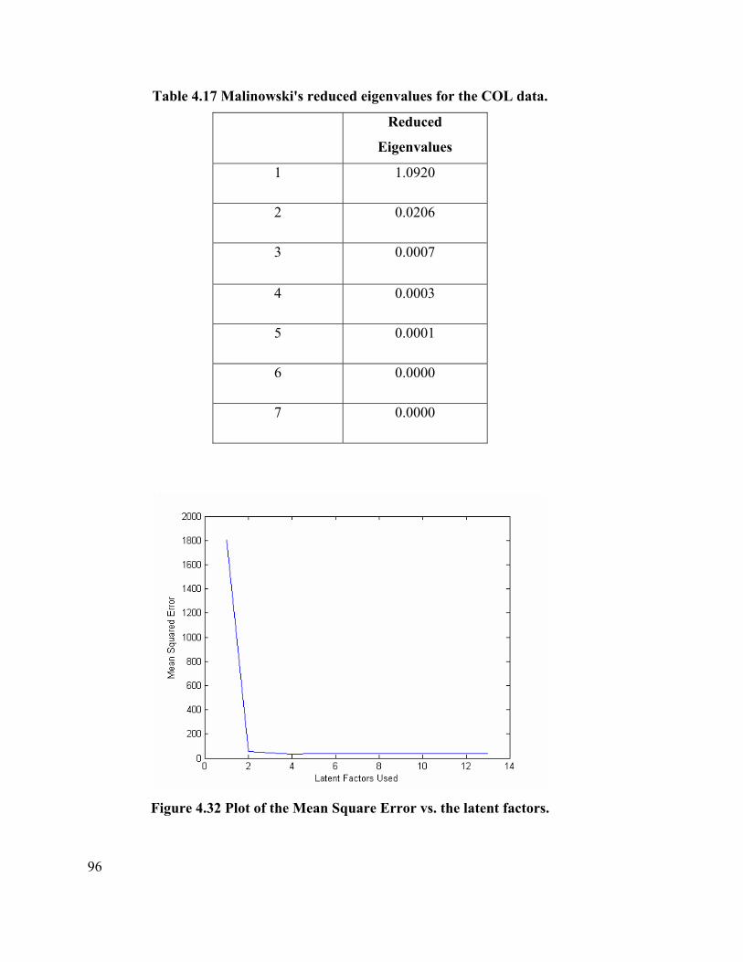
96

Table 4.17 Malinowski's reduced eigenvalues for the COL data.

Reduced

Eigenvalues

1 1.0920

2 0.0206

3 0.0007

4 0.0003

5 0.0001

6 0.0000

7 0.0000

Figure 4.32 Plot of the Mean Square Error vs. the latent factors.

97

Table 4.18 Summary of the PLS results on the COL data set.

PLS R-Sq R-sq-

Adj

MSE RMSE MAE E-

mod.

CN Norm

wt

N

Red. Eig.Val 0.9908 0.9908 57.8274 7.6044 5.8683 0.9094 49.13 1.0215 2

Optimal Val. 0.9946 0.9946 33.9342 5.8253 4.651 0.9278 2311.4 1.029 4

All factors 0.9944 0.9944 35.2658 5.9385 4.7274 0.9266 8940.5 1.3288 7

Figure 4.33 Plots of the Predictions on the test output data using: two, four and all

seven eigen factors.

98

Figure 4.34 Output scores over input scores (predicted and test response) for the

COL data set.

4.3.5 Non-Linear Partial Least Squares (NLPLS) on the COL Data

Two models were built with NLPLS. The first model was built with the optimal number

of factors, and the second was built on [after?] retraining the data. The neural network

training function was used to train the train data set until the performance goal was met.

Using the iterative method, the minimum mean absolute error was computed and plotted

against the latent factor (Figures 4.35 to 4.36). The results showed some inconsistencies.

At the first training, the optimal latent factors value was 4 (Figure 4.35), at the second

training it changed to 2 (Figure 4.36), and in the third training the optimal latent factors

value was 5. These gave three different MAE (see table 4.19).

The results of the three NLPLS models are given in Table 4.19. The model with

only two factors outperformed the one with four factors. The optimal latent factors of 5

(C) gave MSE 22.7752 and MAE of 3.4819. The solution was not stable with NLPLS and

therefore was unreliable. It was observed that when the data were retrained, new optimal

results emerged. This was repeated many times over, and different optimal results were

obtained each time. When two similar optimum factors resulted, the statistics for model

evaluation also differed.

Figure 4.37 shows the plots of the output scores over the input scores for the

predicted and the test response. It is very obvious that there is nonlinearity in the model.

NLPLS also mapped the nonlinearity contained in the data.

99

Figure 4.35 Plot of the MAE against the latent factors after first neural network

training.

Figure 4.36 Plot of the MAE vs. the latent factors for the COL data on another

neural network training.

100

Table 4.19 Summary of the NLPLS results on the COL data. NLPLS R-Sq R-sq-Adj MSE RMSE MAE E-mod. CN Norm

wt

N

4 Lat.Factors.(A) 0.9942 0.9942 36.8616 6.0714 3.4720 0.9457 1 4

2 Lat.Factors (B) 0.9958 0.9958 26.7676 5.1737 3.3850 0.9471 1 2

5 Lat.Factors (C) 0.9964 0.9964 22.7552 4.7702 3.4819 0.9460 1 5


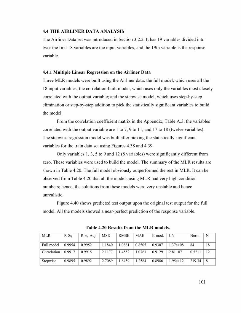
101

4.4 THE AIRLINER DATA ANALYSIS

The Airliner Data set was introduced in Section 3.2.2. It has 19 variables divided into

two: the first 18 variables are the input variables, and the 19th variable is the response

variable.

4.4.1 Multiple Linear Regression on the Airliner Data

Three MLR models were built using the Airliner data: the full model, which uses all the

18 input variables; the correlation-built model, which uses only the variables most closely

correlated with the output variable; and the stepwise model, which uses step-by-step

elimination or step-by-step addition to pick the statistically significant variables to build

the model.

From the correlation coefficient matrix in the Appendix, Table A.3, the variables

correlated with the output variable are 1 to 7, 9 to 11, and 17 to 18 (twelve variables).

The stepwise regression model was built after picking the statistically significant

variables for the train data set using Figures 4.38 and 4.39.

Only variables 1, 3, 5 to 9 and 12 (8 variables) were significantly different from

zero. These variables were used to build the model. The summary of the MLR results are

shown in Table 4.20. The full model obviously outperformed the rest in MLR. It can be

observed from Table 4.20 that all the models using MLR had very high condition

numbers; hence, the solutions from these models were very unstable and hence

unrealistic.

Figure 4.40 shows predicted test output upon the original test output for the full

model. All the models showed a near-perfect prediction of the response variable.

Table 4.20 Results from the MLR models. MLR R-Sq R-sq-Adj MSE RMSE MAE E-mod. CN Norm N

Full model 0.9954 0.9952 1.1840 1.0881 0.8505 0.9307 1.37e+08 84 18

Correlation 0.9917 0.9915 2.1177 1.4552 1.0761 0.9129 2.81+07 0.5211 12

Stepwise 0.9895 0.9892 2.7089 1.6459 1.2584 0.8986 1.95e+12 219.34 8

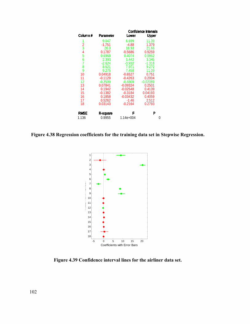
102


RMSE

Parameter

R-square

Lower

F

Upper

P


RMSE

Parameter

R-square

Lower

F

Upper

P


RMSE

Parameter

R-square

Lower

F

Upper

P


RMSE

Parameter

R-square

Lower

F

Upper

P


RMSE

Parameter

R-square

Lower

F

Upper

P


RMSE

Parameter

R-square

Lower

F

Upper

P


RMSE

Parameter

R-square

Lower

F

Upper

P


RMSE

Parameter

R-square

Lower

F

Upper

P


RMSE

Parameter

R-square

Lower

F

Upper

P


RMSE

Parameter

R-square

Lower

F

Upper

P


RMSE

Parameter

R-square

Lower

F

Upper

P

1 9.047 6.699 11.39 2 -1.751 -4.88 1.379 3 20.3 18.93 21.66 4 0.1787 -0.5686 0.9259 5 0.6968 0.4074 0.9862 6 2.393 1.442 3.345 7 -2.624 -3.932 -1.316 8 8.621 7.971 9.272 9 9.275 7.458 11.09

10 0.04918 -0.6527 0.751 11 -0.1129 -0.4263 0.2004 12 -0.2509 -0.4809 -0.02089 13 0.07841 -0.09324 0.2501 14 0.1942 -0.02548 0.4139 15 -0.1382 -0.3184 0.04193 16 0.1858 -0.03432 0.4059 17 0.5262 -1.46 2.512 18 0.03143 -0.2164 0.2793

1.136 0.9955 1.14e+004 0

Figure 4.38 Regression coefficients for the training data set in Stepwise Regression.

-5 0 5 10 15 20

1

2

3

4

5

6

7

8

9

10

11

12

13

14

15

16

17

18


Mod

el T

erm

Num

ber

Figure 4.39 Confidence interval lines for the airliner data set.

103

Figure 4.40 The predicted test output upon the original test outputs.

4.4.2 Principal Component Regression on the Airliner Data

The loadings of the various principal components showed the variables that were

dominant variables in each principal component (PC). This revealed the variables that

were actually significant in each of the selected PCs. Figure 4.41 shows plots of the

loadings for PC1 to PC6. Figure 4.42 shows the loadings for PC7 to PC12 and Figure

4.43 shows the plots of the loadings for PC13 to PC18. Each of the first thirteen PCs has

more than 1% of the explained information on the entire PCs; hence, the rest can be

discarded as noise. Table 4.21 gives the percentage of information explained and its

cumulative for each PC, as well as the dominant variables in that PC.

From Figure 4.41, it can be seen that the first PC carries about 20% of the information

and that the dominant variables in this PC are variables 3, 9, 10, and 12. The second PC

carries about 15% of the information in the total data and the dominant variables are

variables 6, 7, 11, 14, and 17.

Table 4.21 gives the various variables that played dominant roles in each PC. PCs

14 to 18 can be discarded as noise because they do not make up to 1% information.

104

Figure 4.41 The Loadings Vectors vs. the index for the first six PCs showing

dominant variables in each PC.

Figure 4.42 Loadings Vectors vs. index for PCs 7 to 12 showing dominant variables

in each PC.

105

Figure 4.43 Loadings Vectors vs. index for PCs 13 to 18 showing dominant variables

in each PC.

Table 4.21 Percentage explained information and the cumulative Explained. PCs Dominant variables % Explained Cumulative Explained

1 3, 9, 10, 12 20.1088 20.1088

2 6, 7, 11, 14, 17 15.8397 35.9486

3 5 12.1522 48.1008

4 13, 15 8.7710 56.8718

5 4, 15 7.9226 64.7944

6 13 7.1629 71.9573

7 4, 12 6.6275 78.5848

8 5 6.0926 84.6775

9 18 4.9261 89.6035

10 5, 10 3.5530 93.1566

11 11, 12 2.6460 95.8026

12 6, 10 1.4808 97.2834

13 6, 7 1.0571 98.3404

14 9, 14, 16 0.4574 98.7978

15 14 0.4356 99.2334

16 8, 17 0.3599 99.5933

17 1, 2 0.2222 99.8155

18 3, 16 0.1845 100.0000

106

Figure 4.44 is the scree plot of the explained information (eigen values) against

the number of PCs, and PC 10 is a major point of inflection.

Five models were built using the PCR technique. The first was with the first ten PCs; the

second was with the PCs having more than 1% explained information (all PCs with less

than 1% explained information were dropped), leaving thirteen PCs for the model. The

third model was the full model built with all the PCs. The fourth model was built with

scores most correlated with the output variable, and the fifth PC was just an extension of

the fourth. Table 4.22 shows the 19th column of this correlation coefficient matrix. PCs 1

to 4 have scores most closely correlated with the response variable.

Table 4.23 is the summary result of the five PCR models. In terms of MSE, the

full model and the model with 13 PCs were the best in the group. The full model gave the

least MSE, but the condition number was more than 10,000, which is highly unstable and

does not give a unique solution. The model with ten PCs gave a relatively good MSE,

MAE, R2adj, and E-mod, and the condition number was also very good. Hence, it is the

first choice in the PCR, followed by the correlated PCs with 1 to 4 PCs. Figure 4.45

shows a near-perfect prediction for the model built with 10 PCs.

0 2 4 6 8 10 12 14 16 180

10

20

30

40

50

60

Number of PCs

Eig

enva

lues

Figure 4.44 Scree plot of the Eigenvalues against the PCs for the Airliner data.

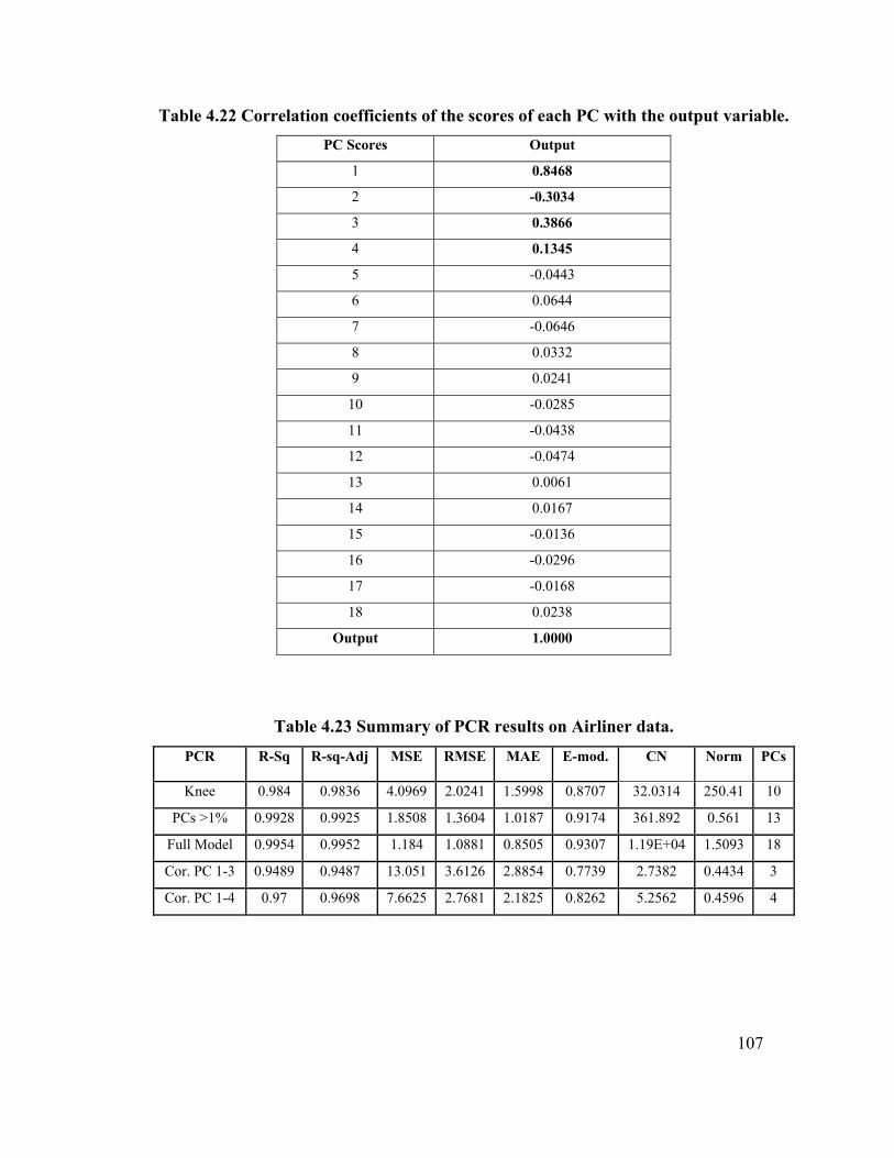
107

Table 4.22 Correlation coefficients of the scores of each PC with the output variable. PC Scores Output

1 0.8468

2 -0.3034

3 0.3866

4 0.1345

5 -0.0443

6 0.0644

7 -0.0646

8 0.0332

9 0.0241

10 -0.0285

11 -0.0438

12 -0.0474

13 0.0061

14 0.0167

15 -0.0136

16 -0.0296

17 -0.0168

18 0.0238

Output 1.0000

Table 4.23 Summary of PCR results on Airliner data.

PCR R-Sq R-sq-Adj MSE RMSE MAE E-mod. CN Norm PCs

Knee 0.984 0.9836 4.0969 2.0241 1.5998 0.8707 32.0314 250.41 10

PCs >1% 0.9928 0.9925 1.8508 1.3604 1.0187 0.9174 361.892 0.561 13

Full Model 0.9954 0.9952 1.184 1.0881 0.8505 0.9307 1.19E+04 1.5093 18

Cor. PC 1-3 0.9489 0.9487 13.051 3.6126 2.8854 0.7739 2.7382 0.4434 3

Cor. PC 1-4 0.97 0.9698 7.6625 2.7681 2.1825 0.8262 5.2562 0.4596 4

108

Figure 4.45 Predicted test output on the original test output.

4.4.3 Ridge regression on the Airliner data

Three ridge regression models were built:

a. ordinary ridge with data not standardized and zero regularization parameter;

b. ridge regression with standardized data and zero regularization parameter; and

c. iterative method using L-curve (norm vs. MSE graph).

The ordinary ridge regression is like the MLR full model and the ridge regression is

similar to the PCR full model. The iterative method of finding the optimal regularization

coefficient (optimal alpha value) uses the singular values to find the range of alpha values

to use in the iteration. The singular values of the Airliner data shown in Table 4.24

ranged from 0 to 52. Using an alpha range of 0 to 1000, the corresponding MSE and

condition numbers were computed. Figure 4.46 is the plot of MSE vs. the regularization

coefficients. This shows the effect of smoothing; while the alpha is increased

(smoothing), the MSE increases. Figure 4.47 shows the regularization coefficients vs. the

weights of the regression coefficients. It shows the relation between Alpha and the

weight. When the alpha was increased, the weight was reduced, so they are inversely

related. This is the same as the relationship between the condition number and alpha. The

MSE vs. weight plot gives the L-curve (Figure 4.48). The optimal alpha value was

chosen from this curve. Norm (weight) values of 0.4 to 0.5 were considered, and a

corresponding alpha value of 6.65 was the optimal at that point.

109

Table 4.24 Singular Value (SV) for the Airliner data. PCs SV

1 51.9924

2 40.9544

3 31.4201

4 22.6779

5 20.4843

6 18.5200

7 17.1359

8 15.7528

9 12.7366

10 9.1865

11 6.8415

12 3.8286

13 2.7331

14 1.1826

15 1.1263

16 0.9304

17 0.5745

18 0.4771

Figure 4.46 MSE vs. Alpha for the Airliner data.

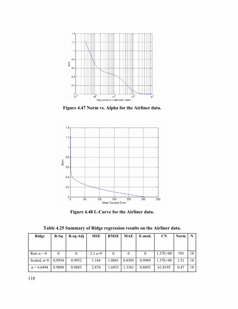
110

Figure 4.47 Norm vs. Alpha for the Airliner data.

Figure 4.48 L-Curve for the Airliner data.

Table 4.25 Summary of Ridge regression results on the Airliner data.

Ridge R-Sq R-sq-Adj MSE RMSE MAE E-mod. CN Norm N

Raw α = 0 0 0 2.1 e+9 0 0 0 1.37E+08 793 18

Scaled, α=0 0.9954 0.9952 1.184 1.0881 0.8505 0.9989 1.37E+08 1.51 18

α = 6.6494 0.9888 0.9883 2.874 1.6953 1.3361 0.8893 61.8195 0.47 18

111

Figure 4.49 Predicted output over the original output.

This alpha value is just below the 11th singular value; hence, 6.8415 was the least

significant singular value. From Figure 4.49A (Predicted output over the original

output), using raw data (unstandardized data), we can see that the prediction was very

bad. Using ridge regression, unstandardized data do not give good predictions. When

standardized with an alpha of zero, the result was the same as with PCR (full model). The

best model, as seen in the Summary Table (Table 4.25), was the model built with an

optimal alpha value of 6.65.

4.4.4 Partial Least Squares (PLS) on the Airliner data

Two PLS models were made in the Airliner data-prediction analysis. The first model was

built from the reduced eigenvalue vs. index plot, where three factors looked significant.

This is shown in Figure 4.50. Using an iterative method Figure 4.51 (MSE vs. latent

factors), the optimal latent factors were found to be 18 (including all the factors).

The summary of the PLS results on the Airliner data is shown in table. The model

with all the factors performed poorly in terms of the condition number and simplicity of

112

the model but was best based on every other criterion of model measurement. On the

other hand, the model with three factors had good condition numbers but a poor MSE as

compared to the MSE with the optimal number of factors.

This iterative method Figure 4.51, which gave the optimal factor number, is

known as the generalization method. It gave the best solution, but the solution is not

unique and is unstable. The first model is preferable because of the stability of the

solution.

The plot of predicted output over the original test output for the Airliner data is

shown in Figure 4.52. The model with full factors looked better than the one with three

factors.

Figure 4.53 is a plot that checks the linearity of the model. It can be observed that

the variables of Airliner data have linear relationship with the output variable; hence, the

output scores plotted over the input scores (predicted and test response) using PLS

followed the same pattern.

Figure 4.50 Plot of reduced eigenvalues against the index.

113

Figure 4.51 MSE vs. latent factors generated from the iterative method.

Table 4.26 Summary of the PLS results on Airliner data.

PLS R-Sq R-sq-Adj MSE RMSE MAE E-mod. CN Norm N

Eig-val. 0.9797 0.9796 5.1856 2.2772 1.8057 0.8547 2.7382 0.4434 3

Optimal 0.9954 0.9952 1.184 1.0881 0.8505 0.9307 1.19e+04 1.5093 18

Figure 4.52 Predicted output over the original test output for Airliner data.

114


4.4.5 Non-Linear Partial Least Squares on Airliner Data

The NLPLS model used the neural network training function to train the training

data set. The plot of MAE and latent factors (Figure 4.54) shows that the optimal latent

factors are 14. On retraining the data, another optimal latent factor is 15. Using both to

build the model, the mean absolute error became 1.2992 and 1.4228. This is shown in the

NLPLS summary table (Table 4.27). The MSEs are 4.0712 and 4.9818, but the condition

numbers are high.

Figure 4.55 shows the NLPLS Airliner scores over the prediction. Toward the

edges (upper and lower parts) of this, prediction lines are seen. This is evidence of over-

fitting. Figure 4.56 reveals the inclusion of nonlinearity in the mapping. In these plots,

output scores were plotted over the input scores (predicted and test response) using

NLPLS. The PLS (see Figure 4.53) gave a good generalization for a linear model, but the

NLPLS did not. The NLPLS model mapped all the information in the data, revealing the

slight presence of a nonlinear relationship between the input variables and the output

variable.

115

Figure 4.54 Plot of MAE against the latent factors.

Table 4.27 NLPLS results on Airliner data. NLPLS R-Sq R-sq-Adj MSE RMSE MAE E-mod. CN Norm N

0.9841 0.9836 4.0712 2.0177 1.2992 0.8959 1.933e+03 14

0.9805 0.9798 4.9818 2.2320 1.4228 0.8878 1.933e+03 15

Figure 4.55 NLPLS scores plotted over the prediction on the Airliner data.

116

Figure 4.56 Plots of the output scores 'U' over the input scores 'T' using NLPLS.

4.5 SIMULATED DATA SET ANALYSIS

The Simulated data set was introduced in the section 3.24. This data set has a total of 44

variables. The response variable is the 38th variable (this occupied the 38th column before

data preprocessing).

4.5.1 Multiple Linear Regression on Simulated Data Set

As with the first three data sets, three ordinary multiple linear regression models were

made:

a. the full Model Regression, which uses all the input variables;

b. the correlation-built model (see correlation coefficient table column 38 in the

Appendix Figure A.4). From the table, variables 8, 9, 15, 17 to19, 21, 23, 24, 26, and

33 to 39 were correlated to the response variable; and

c. the stepwise regression model, which uses the forward (variable addition) or

backward (variable removal) methods to select the most significant variables to build

the model.

Figure 4.57 and Figure 4.58 are the MATLAB stepwise regression outputs

showing the significant variables (solid lines), and the regression coefficients using

the training data.

117

-0.5 -0.4 -0.3 -0.2 -0.1 0 0.1

123456789

10111213141516171819202122232425262728293031323334353637383940414243


Figure 4.57 Confidence interval lines for the training data prediction (Simulated

data set).

Confidence Intervals

Column #

RMSE

Parameter

R-square

Lower

F

Upper

P


RMSE

Parameter

R-square

Lower

F

Upper

P


RMSE

Parameter

R-square

Lower

F

Upper

P


RMSE

Parameter

R-square

Lower

F

Upper

P


RMSE

Parameter

R-square

Lower

F

Upper

P


RMSE

Parameter

R-square

Lower

F

Upper

P


RMSE

Parameter

R-square

Lower

F

Upper

P


RMSE

Parameter

R-square

Lower

F

Upper

P


RMSE

Parameter

R-square

Lower

F

Upper

P


RMSE

Parameter

R-square

Lower

F

Upper

P


RMSE

Parameter

R-square

Lower

F

Upper

P


RMSE

Parameter

R-square

Lower

F

Upper

P


RMSE

Parameter

R-square

Lower

F

Upper

P


RMSE

Parameter

R-square

Lower

F

Upper

P


RMSE

Parameter

R-square

Lower

F

Upper

P

1 -0.001891 -0.01967 0.01589 2 -0.007558 -0.02372 0.008599 3 -0.003061 -0.01921 0.01309 4 0.001641 -0.01971 0.02299 5 -0.00516 -0.02132 0.01099 6 -0.01049 -0.03234 0.01135 7 -0.008518 -0.02998 0.01295 8 -0.1225 -0.3003 0.05534 9 -0.0915 -0.2672 0.08422

10 -0.007261 -0.02341 0.008891 11 9.28e-006 -0.02182 0.02183 12 -0.008757 -0.02654 0.009021 13 -0.007416 -0.02913 0.0143 14 0.00886 -0.01293 0.03065 15 -0.1814 -0.3569 -0.005845 16 -0.01094 -0.02869 0.006808 17 -0.125 -0.2976 0.04761 18 -0.1243 -0.2996 0.0511 19 -0.1285 -0.3045 0.04745 20 -0.002005 -0.01976 0.01575 21 -0.2464 -0.4208 -0.07205 22 -0.008845 -0.03074 0.01305 23 -0.2257 -0.4002 -0.05116 24 -0.2131 -0.3839 -0.0422 25 -0.005165 -0.02296 0.01263 26 -0.1245 -0.3019 0.05297 27 -0.01189 -0.02804 0.004265 28 -0.004968 -0.02269 0.01275 29 -0.002362 -0.02015 0.01543 30 -0.01129 -0.02743 0.004844 31 -0.000544 -0.02229 0.0212 32 0.003535 -0.01807 0.02514 33 -0.19 -0.3593 -0.02072 34 -0.07835 -0.169 0.0123 35 -0.05559 -0.1469 0.03577 36 -0.1488 -0.2353 -0.06238 37 -0.4773 -0.5113 -0.4433 38 -0.1055 -0.192 -0.019 39 -0.1111 -0.1964 -0.02591 40 0.0003324 -0.01583 0.0165 41 -0.002612 -0.01878 0.01355 42 0.003136 -0.01305 0.01933 43 -0.004005 -0.02016 0.01215

0.2482 0.9039 2341 0

Figure 4.58 Regression coefficients and confidence interval ranges for the training

data in stepwise regression on the Simulated data.

118

Table 4.28 Summary of MLR results on the Simulated data set. MLR R-Sq R-sq-Adj. MSE RMSE MAE E-mod. CN Norm N

FULL 0.9065 0.9049 0.0604 0.2458 0.1946 0.6993 9.885e+03 0.5572 43

COR 0.8939 0.8932 0.0685 0.2618 0.2063 0.6825 2.35e+03 0.4962 17

Stepwise 0.8897 0.8876 0.0698 0.2643 0.2081 0.6726 1.083e+03 0.5323 9

Figure 4.59 The predicted test data output MLR on Simulated data set.

The Summary Table showing the results of the MLR on the simulated data set is

given in Table 4.28. The full model was the best in terms of all other measurement

criteria except for the condition number. The condition numbers of the entire three

models were quite high. The MSEs were not significantly different. The plots of the

predicted test data outputs for the three MLR models on the simulated data showed good

predictions.

4.5.2 Principal Component Regression on Simulated Data Set

First, the data were scaled and the reduced singular value decomposition vectors found.

The loadings plots of PCs 1 to 18 are shown in Figures 4.60 to 4.62. These are

representative of the entire loadings. The longest bars in each plot represent the heavy

weights in those PCs. Table 4.29 gives the various PCs with the percentage of explained

information they carry. From this table (Table 4.29), the plots of the explained

information vs. the number of PCs were made. These plots (Figure 4.63) helped to select

the number of significant PCs to retain in the model.

119

For the correlation-built models, Table A.6 in the Appendix gives the output

column of the correlation coefficient matrix of the scores and the output. Coefficients

with absolute values greater than or equal to 0.3 were first considered, and only two PCs

(the 4th and 24th PC) went through. These two were used to build the first correlation PC

model. Then, coefficient values greater than or equal to 0.01 were considered, and

fourteen PCs (PC numbers 1 to 2, 4, 13-18, 20 to 21, and 23 to 25) went through.

In Figure 4.63, there is more than one point of inflection; two models were built

from the first with four PCs and the second with ten PCs. The PCs that had up to 90%

explained information were the first twenty-six PCs, and the PCs that individually had

more than 1% explained information were the first twenty-nine PCs. A model with all the

PCs was also built. Table 4.30 is the Summary Table of the results.

From Table 4.30, Models 3, 4, 5, and 6a were good because they had good MSE,

but Model 5 had a very high condition number (1951.7). Model 3 was the best with 26

PCs (the PCs that had up to 90% of the explained information). The model had the

smallest MSE and the condition number is below 100. Model 3 was better than Model 4

because it looked simpler with 26 PCs, as against 29 PCs in Model 4. The correlation

based model was very close to these two and was also good because, with almost half the

number of PCs of Models 3 and 4, it had a reasonable MSE and condition number.

Figure 4.60 The loadings of PCs 1 to 6 showing the dominant variables in each PC.

120

Figure 4.61 The loadings of PCs 7 to 12 showing the dominant variables in each PC.

Figure 4.62 The loadings of PCs 13 to 18 for the Airliner data showing the dominant

variables in each PC.

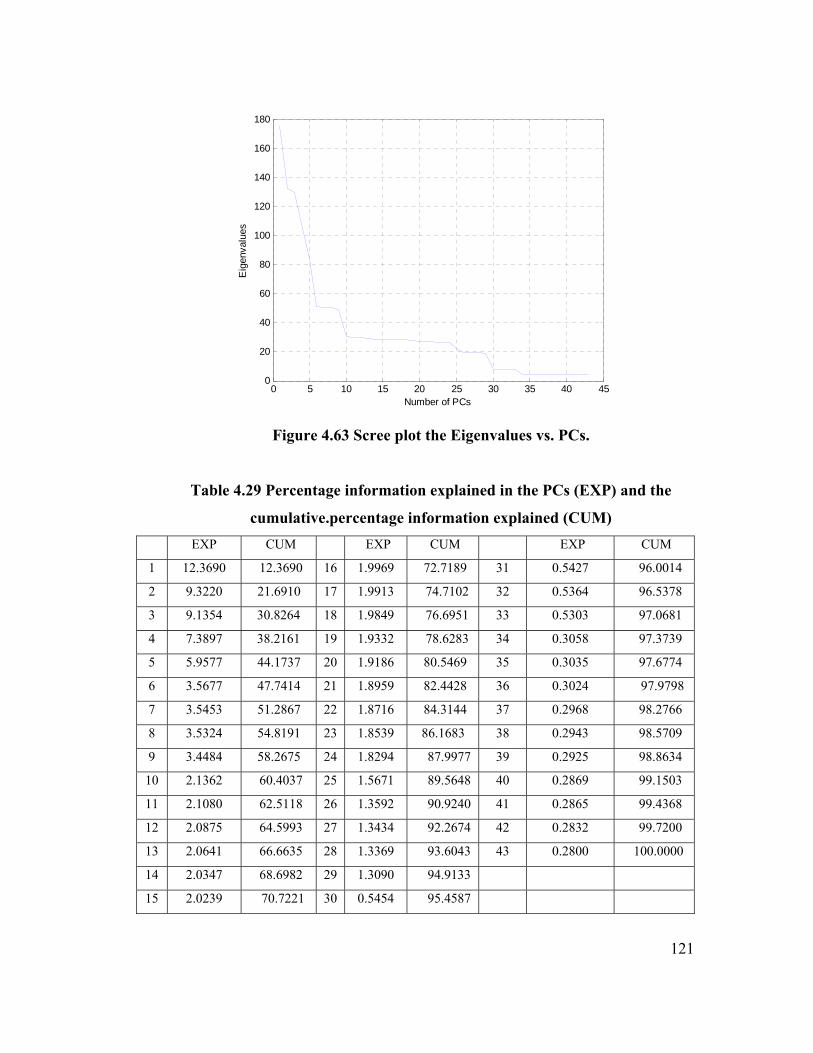
121

0 5 10 15 20 25 30 35 40 450

20

40

60

80

100

120

140

160

180

Number of PCs

Eig

enva

lues

Figure 4.63 Scree plot the Eigenvalues vs. PCs.

Table 4.29 Percentage information explained in the PCs (EXP) and the

cumulative.percentage information explained (CUM) EXP CUM EXP CUM EXP CUM

1 12.3690 12.3690 16 1.9969 72.7189 31 0.5427 96.0014

2 9.3220 21.6910 17 1.9913 74.7102 32 0.5364 96.5378

3 9.1354 30.8264 18 1.9849 76.6951 33 0.5303 97.0681

4 7.3897 38.2161 19 1.9332 78.6283 34 0.3058 97.3739

5 5.9577 44.1737 20 1.9186 80.5469 35 0.3035 97.6774

6 3.5677 47.7414 21 1.8959 82.4428 36 0.3024 97.9798

7 3.5453 51.2867 22 1.8716 84.3144 37 0.2968 98.2766

8 3.5324 54.8191 23 1.8539 86.1683 38 0.2943 98.5709

9 3.4484 58.2675 24 1.8294 87.9977 39 0.2925 98.8634

10 2.1362 60.4037 25 1.5671 89.5648 40 0.2869 99.1503

11 2.1080 62.5118 26 1.3592 90.9240 41 0.2865 99.4368

12 2.0875 64.5993 27 1.3434 92.2674 42 0.2832 99.7200

13 2.0641 66.6635 28 1.3369 93.6043 43 0.2800 100.0000

14 2.0347 68.6982 29 1.3090 94.9133

15 2.0239 70.7221 30 0.5454 95.4587

122

Table 4.30 Summary of PCR results on the Simulated data set. PCR R-Sq R-sq-Adj. MSE RMSE MAE E-mod. CN Norm N

1st knee (1) 0.8102 0.8098 0.1226 0.3501 0.2894 0.5079 12.0198 0.2857 6

2nd knee (2) 0.8101 0.8095 0.1226 0.3502 0.2894 0.5081 33.5263 0.2861 10

=>90%(3) 0.9069 0.906 0.0601 0.2452 0.1943 0.6998 82.8167 0.756 26

PCs >1% (4) 0.907 0.906 0.0601 0.2451 0.1942 0.6998 89.2839 0.7565 29

Full (5) 0.9065 0.9049 0.0604 0.2458 0.1946 0.6993 1951.7 0.7752 43

cor. scores (6a) 0 0 0.6459 0.8037 0.6817 -59.292 45.7169 0.0222 2

cor. scores 6(b) 0.8463 0.8455 0.0993 0.315 0.2503 0.591 62.2957 0.7375 14

4.5.3 Ridge regression on the Simulated data set

Three models were built out of ridge regressions for the Simulated data set. Model (a)

was a model with raw data and zero regularization coefficient (alpha); Model (b) was a

model with scaled data and zero alpha, and Model (c) was a model with scaled data and

varying alpha value including the optimal alpha. For those models with alpha, the

singular values of the data were used to select the alpha range for the iteration method.

Table 4.31 shows the singular values, which ranged from 3 to 176. The optimal alpha can

be neither less than 3 nor greater than 176.

The iterative method of finding the optimal alpha was used to find the minimum

MSE. This was obtained from the MSE vs. Regularization Coefficients plot in Figure

4.64. The relationship between the norm and alpha is also shown in Figure 4.65.

Since the relationship between the condition number and the weights of the regression

coefficients is positive, both quantities were negatively related to the regularization

parameters, as is seen in Figure 4.65, where the weights of the regression coefficient were

negatively related. Smoothing increased the weights of the regression coefficients.

The L-curve in Figure 4.66 helps to locate the optimal alpha value. From the Norm

values region of 0.4 to 0.6, the optimal alpha can be computed. At a norm of 0.5, the

MSE is 0.074. This gave an alpha value of 18.4444.

Using Figure 4.64, the plot of MSE vs. Alpha, the minimum error was 0.0603 and

the alpha value at this MSE value was 3.6055. In Table 4.31, this is below the least alpha

value, 3.9724. This cannot be the optimal alpha value because there is no compromise

123

between the smoothing and MSE. Table 4.32 is the summary of the ridge regression on

the Simulated data set. The best solution, from Table 4.32, was the model built with an

optimal alpha value of 18.44. In this model, there was little compromise between the

smoothing parameter and the bias, MSE. The condition number was reduced from 10,000

to 87. The model built with an alpha value of 3 looked very much like the model with an

alpha value of zero. It can be concluded that at this alpha value, smoothing has not

started. It can also be noticed that both α of 0 and 3.06 looked the same as the full model

MLR and full model PCR (Tables 4.28 and 4.30) with a difference only in the condition

numbers.

Table 4.31 Singular Values (SV) of the Simulated data set. SV SV SV

1 175.4948 16 28.3318 31 7.7001

2 132.2621 17 28.2528 32 7.6104

3 129.6150 18 28.1623 33 7.5244

4 104.8466 19 27.4292 34 4.3385

5 84.5288 20 27.2215 35 4.3062

6 50.6192 21 26.8997 36 4.2905

7 50.3009 22 26.5543 37 4.2115

8 50.1192 23 26.3038 38 4.1752

9 48.9270 24 25.9553 39 4.1504

10 30.3090 25 22.2349 40 4.0708

11 29.9095 26 19.2844 41 4.0647

12 29.6184 27 19.0602 42 4.0181

13 29.2865 28 18.9687 43 3.9724

14 28.8687 29 18.5723

15 28.7156 30 7.7379

124

Figure 4.64 MSE vs. alpha (ridge on the Simulated data).

Figure 4.65 Weight vs. alpha (ridge on the Simulated data).

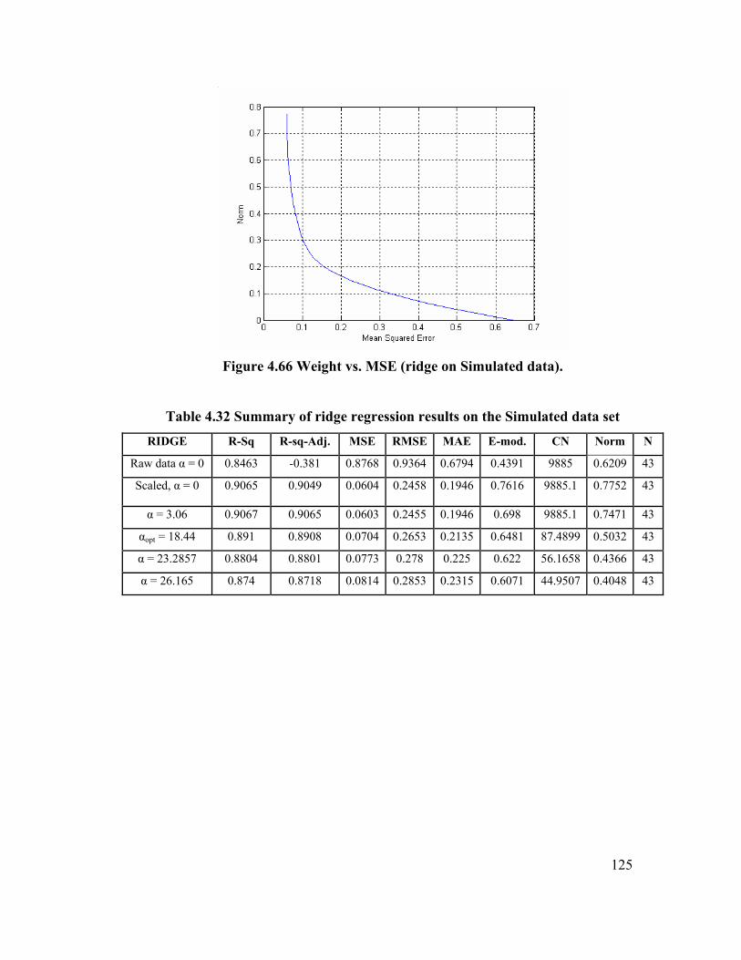
125

Figure 4.66 Weight vs. MSE (ridge on Simulated data).

Table 4.32 Summary of ridge regression results on the Simulated data set

RIDGE R-Sq R-sq-Adj. MSE RMSE MAE E-mod. CN Norm N

Raw data α = 0 0.8463 -0.381 0.8768 0.9364 0.6794 0.4391 9885 0.6209 43

Scaled, α = 0 0.9065 0.9049 0.0604 0.2458 0.1946 0.7616 9885.1 0.7752 43

α = 3.06 0.9067 0.9065 0.0603 0.2455 0.1946 0.698 9885.1 0.7471 43

αopt = 18.44 0.891 0.8908 0.0704 0.2653 0.2135 0.6481 87.4899 0.5032 43

α = 23.2857 0.8804 0.8801 0.0773 0.278 0.225 0.622 56.1658 0.4366 43

α = 26.165 0.874 0.8718 0.0814 0.2853 0.2315 0.6071 44.9507 0.4048 43

126

4.5.4 Partial Least Squares on Simulated Data Set

Four models were built with PLS on the simulated data set. Using Malinowski's reduced

eigenvalues plot (Figure 4.67), the minimum reduced eigen factor is not obvious. Factor

numbers 3 and 5 were used to build models and the results are given in table 4.33 (first

two results in the table). Then the iterative method (generalization) was used to find the

optimal number of factors to get a minimum MSE. Figure 4.68 was used to find the

optimal number of factors. Looking at the plot, at point 8 latent factors, the line touched

the x-axis and ran parallel to that axis. Hence factors 8 and 43 were used to build the

model. The summary of the PLS results is shown in Table 4.33.

From Table 4.33, the best solution using PLS was the model built with the

optimal number of factors (8) from the iterative (generalization) method. It has the best

MSE compared to the others, and the condition number was below 100. Figure 4.69

shows the plot of the internal scores vs. the predicted internal scores. The information in

this data set is linear and the prediction accurately mapped that.

Figure 4.67 Reduced Eigenvalue vs. Index (PLS on Simulated data).

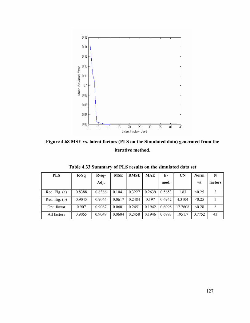
127

Figure 4.68 MSE vs. latent factors (PLS on the Simulated data) generated from the

iterative method.

Table 4.33 Summary of PLS results on the simulated data set

PLS R-Sq R-sq-

Adj.

MSE RMSE MAE E-

mod.

CN Norm

wt

N

factors

Red. Eig. (a) 0.8388 0.8386 0.1041 0.3227 0.2639 0.5653 1.83 <0.25 3

Red. Eig. (b) 0.9045 0.9044 0.0617 0.2484 0.197 0.6942 4.3104 <0.25 5

Opt. factor 0.907 0.9067 0.0601 0.2451 0.1942 0.6998 12.2608 <0.28 8

All factors 0.9065 0.9049 0.0604 0.2458 0.1946 0.6993 1951.7 0.7752 43

128

Figure 4.69 Output scores over input scores (predicted and test response) for PLS

results on the Simulated data set.

4.5.5 Non-Linear Partial Least Squares (NLPLS) on Simulated Data Set

The NLPLS technique uses the neural network training function to train the train data set.

Figure 4.70 is the iterative method of finding the minimum MAE. The optimal number of

factors corresponds to the lowest MAE value. The optimal number of latent factors from

Figure 4.70 was eight. A model with all the factors was also built. Table 4.34 is a

summary of the NLPLS on the Simulated data set. The best NLPLS model was the

optimal factor model built with eight factors; it had a better MSE than the full model and

had a good condition number.

Figure 4.71 shows the internal scores plotted on the predicted internal scores. It

can be seen that the NLPLS mapped nonlinearity in the data into the model. The first

plot, the second plot, and the third plot all revealed some nonlinearity.

Figure 4.72 is the actual prediction on the scores. It is the predicted output on the

original output.

129

Figure 4.70 Mean absolute errors vs. latent factors.

Table 4.34 Summary of the NLPLS results on the Simulated data.

NLPLS R-Sq R-sq-Adj. MSE RMSE MAE E-mod. CN Norm Factors

1st Opt.factors 0.8928 0.8925 0.0692 0.2631 0.208 0.6952 12.2608 8

2nd Opt factors 0.8978 0.8969 0.0664 0.2576 0.2042 0.6971 12.2608 9

All factors 0.8748 0.8726 0.0809 0.2844 0.2162 0.6778 43

Figure 4.71 Internal scores vs. the predicted internal scores (NLPLS on Simulated

data).

130

Figure 4.72 Predicted output on the original output NLPLS on the Simulated data.

131

5.0 GENERAL RESULTS AND CONCLUSION

This chapter gives a conclusion about the various predictive data-mining techniques

discussed in this thesis. It also gives some recommendations for future research in the

area of predictive data-mining techniques, both for the linear and the nonlinear models.

In selecting the best model in the whole group, five measuring criteria were

considered over the nine used in Chapter Four. Models with condition numbers below

100 were chosen first (see section 2.4.2 b). Then, those with the lowest MSE among

those that passed the condition number were chosen. If there were ties, the MAE was

used to break the tie; models with lower MAE were chosen over others. If there was still

a tie, the modified coefficient of efficiency was used, models with higher modified

coefficient of efficiency were favored over others at this stage. Finally, the number of

variables, factors or PCs that made the model was used to select the best model. Models

with fewer variables, factors or PCs were favored over others.

MAE is especially useful in resolving the problem MSE has with outliers. In this

thesis, MSE is not regarded as a better measuring criterion than MAE.

5.1 SUMMARY OF THE RESULTS OF PDM TECHNIQUES

This section gives the summary results of the various techniques used in this Thesis work

and how they performed in each type of data set. It also covers the advantages of each

technique over the other.

5.1.1 Boston Housing Data Results Summary for All the Techniques

From Table 5.1, the best model according to this analysis was Partial Least Squares with

optimal number of factors of 9. This model had a condition number below 100 and the

lowest MSE; only the PLS with three factors was better in terms of MAE. The model

PCR came second, with a CN below 100 and an MSE of 21.1503. The Nonlinear Partial

Least Squares had the lowest MSE, but it mapped linearity into the model. Hence it

cannot be considered a good linear model.

132

Table 5.1 Boston Housing data results summary of all the techniques. Techniques Methods MSE MAE E. mod CN N Ranking

Full 21.1503 3.2500 0.4405 7.33e+07 13

MLR Correlation Coefficient 24.5201 3.4430 0.3645 7.14e+07 11

Stepwise 24.5971 3.3989 0.3809 2.122e+7 6

Full 21.1503 3.250 0.4405 87.5639 13

90% variation 23.5042 3.3517 0.3948 31.935 11

PCR 1st Knee 25.3053 3.4919 0.3432 7.1561 4

2nd knee 23.3328 3.3714 0.3833 29.7520 10

Correlation Coefficient (1-3) 27.1818 3.5908 0.3393 7.1561 3

Correlation Coefficient (1-5,

12) 22.5133 3.3975 0.3919 36.3902 6

2nd

Raw Data, α = 0 340100 460 0.000 7.3e+07 13

Raw Data, α = 72 4414.7 2331.6 13

RIDGE Scaled Data,α = 0 23.5042 3.3517 0.3948 31.9635 13

Scaled Data,α =1 21.1576 3.2429 0.4396 82.8704 13

Scaled Data, α =4.1 21.6261 3.2255 0.4166 45.1361 13

Reduced Eigen factors (a) 23.0754 3.3019 0.3952 <7 2

Reduced Eigen factors (b) 22.0992 3.2433 0.4204 7.2 3

PLS Minimum Eigenvalue 21.5159 3.2928 0.4360 <36 5

Optimal Factors 21.1395 3.2498 0.4408 <29 9

All Factors 21.1503 3.2500 0.4405 87.5639 13

1st

NLPLS Optimal Factors 17.9547 2.9545 0.5121 4

All Factors

133

5.1.2 COL Data Results Summary for All the Techniques

The COL is a highly ill-conditioned data set. The best model for this data set is the Partial

Least Squares (PLS), built with two factors (see Table 5.2). Among all the models that

are below the condition number of 100, it has the best MSE and MAE. The second best is

the PCR model with only two PCs. It has MSE lower than the group that survived the

condition number elimination.

Again, the NLPLS gave the best model if MSE is the only criterion for comparison. It can

be seen that the solution is not stable. It has three optimal solutions. Each time the model

was retrained, a new optimal solution is obtained. It mapped nonlinearity into the model

and hence can only be useful if a nonlinear model is being considered.

5.1.3 Airliner Data Results Summary for All the Techniques

The best model for the Airliner data was the ridge regression with a regularization

parameter of 6.65 (see Table 5.3). It is best in the group with a condition number less

than 100 and an MSE of 2.874 which, is better than all the other models that passed the

condition number elimination. This model is followed by the PCR model with 10 PCs.

The NLPLS did not perform as well as the PLS in this data set using MSE but using

MAE gave better.

5.1.4 Simulated Data Results Summary for All the Techniques

The Simulated data set with many input variables has the PLS with optimal

factors as the best model for prediction. This is followed by the PCR model with 29 PCs.

Both models gave the same measurements, but the PLS came up better by the number of

factors used in the model. It used only 8 out of 43 factors for its prediction.

The NLPLS also mapped nonlinearity into the model. This is not good because the

relationship of the regression is a linear one.

134

Table 5.2 COL data Results Summary for all the techniques. Techniques Methods MSE MAE E. mod CN N Ranking

Full 35.2658 4.7274 0.9266 4.24e+06 7

MLR Correlation Coefficient. 35.2658 4.7274 0.9266 4.24e+06 7

Stepwise 35.2658 4.7274 0.9266 4.24e+06 7

1st Knee 63.5893 6.1286 0.9053 49.1301 2

90% variation 64.4823 6.1520 0.9053 2311.4 3

PCR Correlation Coefficient. 63.5893 6.1286 0.9053 49.1301 2

<1% variation out 36.6783 4.7118 0.9270 2767.1 6

All PCs (Full mod.) 35.2658 4.7274 0.9266 8940.5 7

2nd

Raw Data, α = 0 3.3e+09 10,000 0.0000 4.2e+06 7

Raw Data, α = 373 1.92e+07 4.4e+03 7

RIDGE Scaled Data,α = 0 35.2658 4.7274 0.9909 8.9e+03 7

Scaled Data,α = 3.6 33.0698 4.6334 0.9279 1965.6 7

Scaled Data, α = 9 54.5487 5.7354 0.9093 382.6858 7

Reduced Eigen Factors 57.8274 5.8683 0.9094 49.130 2

PLS Optimal Factors 33.9342 4.6510 0.9278 2311.4 4

Al Factors 35.2658 4.7274 0.9266 8940.5 7

1st

Optimal factors 26.7676 3.3850 0.9471 2


Optimal Factors 22.7552 3.4819 0.9460 5

All Factors 26.7676 3.3850 0.9471 7

135

Table 5.3 Summary of the Results of All the Techniques on Airliner Data . Techniques Methods MSE MAE E. mod CN N Ranking

Full 1.1840 0.8505 0.9307 1.37e+08 18


Stepwise 2.7089 1.2584 0.8986 1.95e+12 8

1st knee and 90% 4.0969 0.5998 0.8707 32.0314 10

<1% variation out 1.8508 1.0187 0.9174 362 13

PCR Full 1.1840 0.8505 0.9307 1.89e+04 18

Correlation Coefficient (1-

3) 13.0509 2.8854 0.7739 2.7382 3

Correlation Coefficient (1-

4) 7.6625 2.1825 0.8262 5.2562 4

Raw Data, α = 0 2.1e+09 0.0000 0.0000 1.37e+08 18

RIDGE Scaled Data,α = 0 1.1840 0.8505 0.9989 1.19e+04 18

Scaled Data, α = 6.65 2.8740 1.3361 0.8893 61.8195 18

1st

PLS Reduced Eigen Factors 5.1856 1.8057 0.8547 2.7382 3

All Factors/optimal 1.1840 0.8505 0.9307 1.19e+04 18

2nd


All Factors

136

Table 5.4 Summary of the Results of Simulated data for all the techniques. Techniques Methods MSE MAE E. mod CN N Ranking

Full 0.0604 0.1946 0.6993 9.885e+03 43


Stepwise 0.0698 0.2081 0.6726 1.083e+03 9

1st Knee 0.1226 0.2894 0.5079 12.0198 6

2nd knee 0.1226 0.2894 0.5081 33.5263 10

PCR =>90% variation 0.0601 0.1943 0.6998 82.8167 26

<1% variation out 0.0601 0.1942 0.6998 89.2839 29

All PCs (Full mod.) 0.0604 0.1946 0.6993 1951.7 43

Correlation Coefficient (a) 0.6459 0.6817 -0.5929 45.7169 2

Correlation Coefficient (b) 0.0993 0.2503 0.5910 62.2957 14

2nd

Raw Data, α = 0 0.8768 0.6794 0.4391 9885.1 43

RIDGE Scaled Data, α = 0 0.0604 0.1946 0.7616 9885.1 43

Scaled Data, α =3.06 0.0603 0.1946 0.6980 9885.1 43

Scaled Data, αopt =18.44 0.0704 0.2135 0.6481 87.4899 43

Scaled Data, α = 23.286 0.0773 0.2250 0.6220 56.1658 43

Scaled Data, α = 26.165 0.0814 0.2315 0.6071 44.9507 43

Reduced Eigen Factors 0.1041 0.2639 0.5653 1.83 3

PLS Reduced Eigen Factors 0.0617 0.1970 0.6942 4.3104 5

Optimal Factors 0.0601 0.1942 0.6998 12.2608 8

Al Factors 0.0604 0.1946 0.6993 1951.7 43

1st


All Factors 0.0809 0.2162 0.6778 43

137

5.2 CONCLUSION

In conclusion, in the course of this work, the various data preprocessing techniques were

used to process the four data sets introduced in Chapter Three (Methodology). Some of

the data sets were seen to have unique features; an example is the COL data set, which is

very collinear. This helped in the division of the data in Chapter Four. In Chapter Four,

all the five predictive data-mining techniques were used to build models out of the four

data sets, and the results from the various methods were summarized. In this chapter, the

results from these techniques will be globally compared.

PLS generally performed better than all the other four techniques in building

linear models. It dealt with the collinearity in the COL data and gave the simplest model

that made the best predictions. The PLS also reduced the dimensionality of the data. The

study shows that supervised techniques demonstrated a better predictive ability than

unsupervised techniques. It can be seen that in MLR and PCR, the correlation-based

models which were supervised techniques performed reasonably better than most models

where variables and PCs were randomly selected to build the model. The variables that

added valuable information to the prediction models were variables that had correlation

with the output being predicted.

Ridge regression also did very well with the ill-conditioned Airliner data. It

reduced the condition number of the data matrix from 137,000,000 to just 62 with very

little compromise on the MSE (bias). It also performed better than most on the COL data:

the condition number was pulled down from 4,000,000 to just 383, and it was beaten only

by PLS with two factors.

From the analysis, it can be seen that the condition number of any data matrix has

a direct relation to the number of statistically significant variables in the model.

Based on the results from the Summary Tables and the discussion so far on the

predictive linear modeling techniques, Tables 5.5 to 5.8 itemize a general comparison of

all the models, along with their advantages and limitations.

138

Table 5.5 Linear models compared with non-linear partial least squares. LINEAR MODELS NLPLS

1 Models only linear relationship Models both linear and non-linear relationship

2 Computationally less expensive Computationally more expensive

3 Good for linear models only Good for linear models and models containing

about 20% non-linearity

4 For some collinear data, performs better Can give unstable results (see COL data analysis)

5 Good generalization for linear models. Cannot give good generalization for linear models

because it maps non-linearity into the model.

Table 5.6 Comparison of MLR with PCR, PLS and Ridge regression techniques.

MLR/OLS PCR, PLS, RIDGE

1 No standardization or scaling required Standardization or scaling needed

2 Gives good predictions when the inputs variables are truly independent

Predicts better when input variables are not independent of each other.

3 Good when the input variables are all useful in predicting the response

Better when there need for variable reduction. except for ridge.

4 Computationally inexpensive Computationally expensive

5 Simpler to understand and interpret More complex in its solutions

6 Most times results in large regression coefficients

Regression coefficients are much lesser

7 Sometimes gives unstable results most times gives stable results but may give a solution that is not representative of the matrix being modeled

8 Does not take care of ill-conditioned data or collinear data

Does better with ill-conditioned or collinear data

9 Does not take care of Collinear data Removes collinearity

10 Not better when there are many redundant variables in the input.

Better for dimensionality reduction or feature selection

11 maximizes the squared correlation between projected inputs and output

PLS maximizes the covariance between projected inputs and output, PCR maximizes variance of the projected inputs, Ridges works same like OLS but uses regularization parameter to reduce the regression weights.

12 Minimizes the output prediction error to perform well

same

13 Linear models have fixed shape linear basic function

same

14 Not easy to detect presence of non-linearity in the model

Easy to detect using the scores from the PCA.

139

Table 5.7 PCR compared with PLS PCR PLS

1 Transforms data into orthogonal space Same

2 Considers only input variables in its

transformation

Considers both input and output variables in its

transformation

3 Unsupervised technique Supervised technique

4 Less complex computation More complex computation

5 Takes care of collinear data prediction A better prediction model for collinear data set

6 Gives good prediction model makes better prediction model

Table 5.8 PLS/PCR compared with Ridge. PLS/PCR RIDGE

1 Uses Standardized or scaled data same

2 Transforms data into orthogonal space Does not transform data

3 Takes care of collinearity Takes care of collinearity

4 Removes collinearity by transforming

data into orthogonal space

Removes collinearity by using regularization

coefficients

5 Performs well with collinear problem Always work well with collinear problem

6 Easy to detect non-linearity in the model Not easy to detect.

7 Results is dependent on the number of

PCs, factors

Uses full variables all the time but result dependent

on the regularization parameter

8 Deals with ill-conditioned regression

problems by dropping PCs associated

with small eigen values

Damps the minor components

9 truncates singular values when there is

clear gap between two eigenvalues

works well when there is no clear gap between two

eigenvalues

140

5.3 RECOMMENDATIONS FOR FUTURE WORK

Some predictive data-mining problems are of the non-linear type. For very complex

prediction (or forecasting) problems, non-linear algorithms or a blend of both linear and

non-linear will be best. This means blends of different algorithms or techniques which

combine strengths will be more useful. Effort should be geared towards building super

models that combines two or more of these techniques. A great deal of works is going on

in evaluating the strengths of the techniques: the neural network (NN), support vector

regression (SVR), the regression trees, kernel regression, kernel SVR and so on. Some of

the breakthroughs are the kernel support vector machines, the kernel PCA and the least

square support vector machines.

Another area of data-mining that has been and will continue to be a fertile ground for

researchers is the area of data acquisition and storage. The ability to correctly acquire,

clean, and store data sets for subsequent mining is no small task. A lot of work is going

on in this area to improve on what is obtainable today.

There are many commercial software packages produced to solve some of these

problems but most are uniquely made to solve particular types of problem. It would be

desirable to have mining tools that can switch to multiple techniques and support multiple

outcomes. Current data-mining tools operate on structured data but most of the data in the

field are unstructured. Since large amount of data are acquired, for example in the World

Wide Web, there should be tools that would manage and mine data from this source, a

tool that can handle dynamic data, sparse data, incomplete or uncertain data. The dream

looks very tall but given the time and energy invested in this field and the results which

are produced, it will not be long to get to the development of such softwares.

141

LIST OF REFERENCES

142

LIST OF REFERENCES

1. Lyman, P., and Hal R. Varian, "How much storage is enough?" Storage, 1:4

(2003).

2. Way, Jay, and E. A. Smith,"Evolution of Synthetic Aperture Radar Systems and

Their Progression to the EOS SAR," IEEE Trans. Geoscience and Remote

Sensing, 29:6 (1991), pp. 962-985.

3. Usama, M. Fayyad, "Data-Mining and Knowledge Discovery: Making Sense

Out of Data," Microsoft Research IEEE Expert, 11:5. (1996), pp. 20-25.

4. Berson, A., K. Thearling, and J. Stephen, Building Data Mining Applications for

CRM, USA, McGraw-Hill (1999).

5. Berry, Michael J. A. et al., Data-Mining Techniques for Marketing, Sales and

Customer Support. U.S.A: John Wiley and Sons (1997).

6. Weiss, Sholom M. et al., Predictive Data-Mining: A Practical Guide. San

Francisco, Morgan Kaufmann (1998).

7. Giudici, P., Applied Data-Mining: Statistical Methods for Business and Industry.

West Sussex, England: John Wiley and Sons (2003).

8. Berry, M. J. A., and G. S. Linoff, Mastering Data Mining. New York: Wiley

(2000).

9. Han, J., and M. Kamber, Data Mining: Concepts and Techniques. New York:

Morgan Kaufman (2000).

10. Pregibon, D., "Data Mining," Statistical Computing and Graphics, pp. 7-8.

(1997).

11. Usama, M. Fayyad, et al., Advances in Knowledge Discovery and Data Mining.

Cambridge, Mass.: MIT Press (1996).

12. Ralph, Kimball, The Data Warehouse Toolkit: Practical Technique for Building

Dimensional Data Warehouses. New York: John Wiley (1996).

13. Betts, M., "The Almanac: Hot Tech," ComputerWorld 52 (Nov. 17, 2003).

14. Goth, Greg., "E-Voting Milestones," IEEE Security and Privacy, 2:1 (2004), p.

14.

143

15. Chapman, P. et al., "CRISP-DM 1.0: Step by Step Data Mining Guide," CRISP-

DM Consortium http://www.crisp-dm.org (2000).

16. Pyzdek, Thomas, The Six Sigma Handbook, Revised and Expanded. New York:

McGraw-Hill (2003).

17. Koh, Chye Hian, and Kee Chan Low, "Going Concern Prediction Using Data

Mining Techniques." Managerial Auditing Journal, 19:3 (2004).

18. Austerlitz, Howard., Data Acquisition Techniques Using PCS. USA: Elsevier

(2003).

19. Caristi, A. J., IEEE-488 General Purpose Instrument Bus Manual. London:

Academic Press (1989).

20. Klaassen, B. Klaas., Electronic and Instrumentation. New York: Cambridge

University Press (1996).

21. Hansen, P. C., "Analysis of discrete ill-posed problems by means of the L-

Curve," SIAM Reviews, 34:4 (1992), pp. 561-580

22. Hines, J. Wesley, Advanced Monitoring and Diagnostic Techniques, NE 579

(Summer 2005).

23. Pyle, Dorian, Data Preparation for Data-Mining. San Francisco, Morgan

Kaufmann (1999).

24. Gencay, Ramazan, and F. Selcuk, An Introduction to Wavelets and other

Filtering Methods in Finance and Economics. San Diego, CA: Elsevier

(2002).

25. Olaf, Rem, and M. Trautwein, "Best Practices Report Experiences with Using

the Mining Mart System." Mining Mart Techreport. No. D11.3 (2002).

26. Kassams Lee Yong, "Generalized Median Filtering and Related Nonlinear

Techniques," IEEE Transactions on Signal Processing, 33:3 (1985), pp.

672-683.

27. Agresti, Alan, Categorical Data Analysis, 2nd edition. Hoboken, New Jersey:

Wiley Interscience (2002).

28. Douglas C.M, and C. R. George, Applied Statistics and Probability for

Engineers, 3rd edition. New York: John Wiley (2002).

144

29. Elisseeti, Isabelle., "An Introduction to Variable and Feature Selection," The

MIT Press Journals. 3:7-8 (2003).

30. Morison, D. F., Multivariate Statistical Methods, 2nd Edition. New York:

McGraw-Hill (1976).

31. Seal, H., Multivariate Statistical Analysis for Biologists, London: Methuen

(1964).

32. Webster’s Revised Unabridged Dictionary. Springfield, Mass.: C. and G.

Merriam, Co., Revised (1998).

33. Bishop, C.M., Neural Networks for Pattern Recognition, Oxford, UK: Oxford

University Press (1995).

34. Johnson, D.E., Applied Multivariate Methods for Data Analysis, Pacific Grove

CA: Brooks/Cole (1998).

35. Jolliffe, I.T., Principal Component Analysis, New York: Springer-Verlag (1986).

36. Cohen, Jacob, et al., Applied Multiple Regression/Correlation Analysis for the

Behavioral Sciences. Mahwah, New Jersey: Lawrence Erlbaun Asso.

(2003).

37. Walpole, R.E, S.L Myers, and K. Ye., Probability and Statistics for Engineers

and Scientists, 7th edition. Englewood Cliffs, NJ: Prentice Hall (2002).

38. Green, P., and B. Silverman, Non-Parametric Regression and Generalized

Linear Models, London: Chapman-Hall (1994).

39. Lewis-Beck, and S. Michael, Applied Regression: An Introduction, Newbury

Park, CA: Sage Publication, Inc. (1980).

40. Kish, Leslie, Statistical Design for Research, New York: John Wiley (1987).

41. Watkins, S. David, Fundamentals of Matrix Computations, New York: John

Wiley (1991).

42. Kline, Rex B., Principle and Practice of Structural Equation Modeling, 2nd

edition. New York: Guilford Press (2005).

43. Berk, Kenneth, N., "Tolerance and Condition in Regression Computations,"

Journal of American Statistical Association, 72: 360 (Dec. 1977), pp. 865-

866.

145

44. Draper, N., and H. Smith, Applied Regression Analysis, 2nd edition. New York:

John Wiley (1981), pp. 307-312.

45. Dash, M., and H. Liu, "Feature Selection for Classification," Intelligent Data

Analysis. 1:3 (1997) pp. 131-156.

46. Naes, T., and H. Martens, "Principal Component Regression in NIR Analysis:

Viewpoints, Background Details and Selection of Components," J.

Chemom. 2 (1988), pp. 155-167.

47. Jeffers, J. N. R., "Two Case Studies in the Application of Principal Component

Analysis," Applied Statistics, 16 (1967) pp. 225-226.

48. Sun, J., "A correlation Principal Component Regression Analysis of NIR." J.

Chemom 9 (1995), pp. 21-29.

49. Ferre, J. and F. X. Rius, "Selection of the Best Calibration Sample Subset for

Multivariate Regression." Anal. Chem 68 (1996), pp. 1565-1571.

50. Davies, A.M.C., “The Better Way of Doing Principal Component Regression,”

Spectroscopy Europe 7 (1995), pp. 36-38.

51. Hoerl, A. E., "Application of Ridge to Regression Problems," Chemical

Engineering Progress, 58 (1962), pp. 54-59.

52. Tikhonov, A. N., "Solution to Incorrectly Formulated Problems and the

Regularization Method," Soviet Math DokI 4, 1035-1038, English

Translation of DokI Akod Nauk SSSR 151, 501-504 (1963).

53. Trevor, H., T. Robert, and F. Jerome, The Elements of Statistical Learning, New

York: Springer-Verlag (2002).

54. Morozov, V.A., Methods for solving incorrectly posed problems, New York,

Springer Verlag, (1981).

55. Mallows, C.L., "Some Comments on Cp" Technometrics, 15 (1973), pp. 661-

675.

56. Sugiyama, Masashi, "Estimating the Error at Given Test Inputs for Linear

Regression," Neural Networks and Intelligence NCI. Proceedings 413.

(2004).

146

57. Golub, Gene H., Michael Heath, and Grace Wahba, "Generalized Cross-

Validation as a Method for Choosing a Good Ridge Parameter,"

Technometrics, 21:2. (May 1979).

58. Wu, Limin, "A Parameter Choice Method for Tikhonov Regularization,"

Electronic Transaction on Numerical Analysis, 16 (2003), pp. 107-128.

59. Groetsch, C. W., "The theory of Tikhonov Regularization for Fredholm

Equations of The First Hand," Research Notes in Mathematics. Boston,

Pitman (1984), p. 105.

60. Hardle, W., Smoothing Techniques, New York, Springer-Verklag. (1990).

61. Garthwait, H. Paul, "An Interpretation of Partial Least Squares," Journal of

American Statistical Association, 89:425 (1994), pp. 122-127.

62. Malinowski, E. R., "Determination of the Number of Factors and The

Experimental Error in a Data Matrix." Anal. Chem. 49 (1977), pp. 612-

617.

63. Sharma, K. Sanjay, et al., "A Covariance-Based Nonlinear Partial Least Squares

Algorithm," Intelligent Systems and Control Research Group (2004).

64. Frank, I. E., "A Nonlinear PLS Model," Journal of Chemometrics and Intelligent

Laboratory Systems, 8 (1990) pp. 109-119.

65. Bakshi R. Bhavik, and Utomo Utojo, "A Common Framework for the

Unification of neural, Chemometric, and Statistical modeling methods,"

Analytica Chimica Acta 384 (1999), pp. 227-274.

66. Munoz, Jesus, and Angel M. Felicisimo, "Comparison of Statistical Methods

Commonly used in Predictive Modeling," Journal for Vegetations Science

15 (2004), pp. 285-292.

67. Specht, D. F., "A General Regression Neural Network," IEEE Transactions on

Neural Networks, 2:6 (1991), pp. 568-576.

68. Manel, S., J. M. Dias, and S. J. Ormerod, "Comparing Discriminant Analysis,

Neural Networks and Logistic Regression for Predicting Species

Distribution: A Case Study with a Himalayian River Bird," Ecol. Model.

120 (1999), pp. 337-347.

147

69. Frank, I.E., and J. H. Friedman, "A Statistical View of Some Chemometrics

Regression tools," Technometrics, 35: 2 (1993), p. 109.

70. Lorber, A., L. E. Wangen, and B. R. Kowalski, "A Theoretical Foundation for

the PLS Algorithm" J. Chemom, 1, 19. (1987).

71. Stone, M., and R. J. Brooks, "Continuum Regression: Cross-Validated

Sequentially Constructed Prediction Embracing Ordinary Least Squares

and Principal Component Regression,"J. Royal Statistical Society, Serial

B. 52, 175. (1984).

72. Elder, John F [IV] and D. W. Abbott, "A Comparison of Leading Data Mining

Tools," Fourth International Conference on Knowledge Discovery and

Data Mining. http://www.datamininglab.com. New York (1998).

73. Widrow, B., and M. A. Lehr, "30 Years of Adaptive Neural Networks:

Perceptron, Madaline and Backpropagation," Proceedings of the IEEE,

78:9 (1990), pp. 1415-1442.

74. Battaglia, Glenn J., and James M. Maynard, "Mean Square Error: A Useful Tool

for Statistical Process Management," AMP Journal of Technology 2

(1996), pp. 47-55.

75. Berry, Michael J. A., et al., Data Mining Techniques for Marketing, Sales and

Customer Relationship Management. Indianapolis, USA, John Wiley and

Sons (2004).

76. Legates, David R. and Gregory J. McCabe, "Evaluating the Use of Goodness of

Fit Measures in Hydrologic and Hydroclimatic Model Validation." Water

Resources Research, 35:233-241 (1999).

77. Nash, J.E. and J.V. Sutcliffe, "Riverflow Forecasting through Conceptual

Models: Part 1-A Discussion of Principles." J. Hydrology, 10 (1970), pp.

282-290.

78. Willmott, C.J., S.G. Ackleson, R.E. Davis, J.J. Feddema, K.M. Klink, D.R.

Legates, J. O'Donnell, and C.M. Rowe, "Statistics for the evaluation and

comparison of models." J. Geophy. Research 90 (1985), pp. 8995-9005.

148

79. Xie, Y.-L, and J.H. Kaliva, "Evaluation of Principal Component Selection

Methods to form a Global Prediction Model by Principal Component

Regression," Analytica Chemica Acta, 348:1 (Aug. 1997) pp. 19-27.

80. Farkas, Orsolya, and Heberger Karoly, "Comparison of Ridge Regression, PLS,

Pairwise Correlation, Forward and Best Subset Selection methods for

Prediction of Retention indices for Aliphatic Alcohols," Journal of

Information and Modeling, 45:2 (2005) pp. 339-346.

81. Huang, J. et al., "A Comparison of Calibration Methods Based on Calibration

Data size and Robustness," Journal of Chemometrics and Intelligent Lab.

Systems, 62:1 (2002) pp. 25-35.

82. Vigneau, E., M. F. Devaux, and P. Robert, "Principal Component Regression,

Ridge Regression, Ridge Principal Component Regression in

Spectroscopy Calibration," Journal of Chemometrics, 11:3 (1996) pp. 239-

249.

83. Malthouse, Edward C., "Ridge Regression and Direct Marketing Scoring

Models," Journal of Interactive Marketing, 13:1854 (2000), pp. 16-23.

84. Basak, Subhash C. et al., "Prediction of Human Blood: Air Partition Coefficient:

A Comparison of Structure-based and Property-based Methods," Journal

of Risk Analysis, 23:6 (2003), pp. 1173.

85. Naes, T., C. Irgens, and H. Martens, "Comparison of Linear Statistical Methods

for Calibration of NIR Instruments," Applied Statistics, 35:2 (1986), pp.

195-206.

86. Hines, J. W., Personal Communication, University of Tennessee at Knoxville,

Fall 2005.

149

APPENDICES

150

APPENDIX A

Table A.1 Boston Housing Data Correlation coefficient Matrix

Col 1 Col 2 Col 3 Col 4 Col 5 Col 6 Col 7 Col 8 Col 9 Col 10 Col 11 Col 12 Col 13 Col 14

1 -0.2005 0.4066 -0.0559 0.421 -0.2192 0.3527 -0.3797 0.6255 0.5828 0.2899 -0.3851 0.4556 -0.3883

-0.2005 1 -0.5338 -0.0427 -0.5166 0.312 -0.5695 0.6644 -0.3119 -0.3146 -0.3917 0.1755 -0.413 0.3604

0.4066 -0.5338 1 0.0629 0.7637 -0.3917 0.6448 -0.708 0.5951 0.7208 0.3832 -0.357 0.6038 -0.4837

-0.0559 -0.0427 0.0629 1 0.0912 0.0913 0.0865 -0.0992 -0.0074 -0.0356 -0.1215 0.0488 -0.0539 0.1753

0.421 -0.5166 0.7637 0.0912 1 -0.3022 0.7315 -0.7692 0.6114 0.668 0.1889 -0.3801 0.5909 -0.4273

-0.2192 0.312 -0.3917 0.0913 -0.3022 1 -0.2403 0.2052 -0.2098 -0.292 -0.3555 0.1281 -0.6138 0.6954

0.3527 -0.5695 0.6448 0.0865 0.7315 -0.2403 1 -0.7479 0.456 0.5065 0.2615 -0.2735 0.6023 -0.377

-0.3797 0.6644 -0.708 -0.0992 -0.7692 0.2052 -0.7479 1 -0.4946 -0.5344 -0.2325 0.2915 -0.497 0.2499

0.6255 -0.3119 0.5951 -0.0074 0.6114 -0.2098 0.456 -0.4946 1 0.9102 0.4647 -0.4444 0.4887 -0.3816

0.5828 -0.3146 0.7208 -0.0356 0.668 -0.292 0.5065 -0.5344 0.9102 1 0.4609 -0.4418 0.544 -0.4685

0.2899 -0.3917 0.3832 -0.1215 0.1889 -0.3555 0.2615 -0.2325 0.4647 0.4609 1 -0.1774 0.374 -0.5078

-0.3851 0.1755 -0.357 0.0488 -0.3801 0.1281 -0.2735 0.2915 -0.4444 -0.4418 -0.1774 1 -0.3661 0.3335

0.4556 -0.413 0.6038 -0.0539 0.5909 -0.6138 0.6023 -0.497 0.4887 0.544 0.374 -0.3661 1 -0.7377

-0.3883 0.3604 -0.4837 0.1753 -0.4273 0.6954 -0.377 0.2499 -0.3816 -0.4685 -0.5078 0.3335 -0.7377 1

150

151

Table A.2 Col Data Correlation Coefficient Matrix

Col 1 Col 2 Col 3 Col 4 Col 5 Col 6 Col 7 Col 8

1.0000 0.9832 0.9817 0.9763 0.9789 0.8493 0.9912 0.8342

0.9832 1.0000 0.9986 0.9923 0.9959 0.8678 0.9809 0.8528

0.9817 0.9986 1.0000 0.9934 0.9955 0.8591 0.9814 0.8468

0.9763 0.9923 0.9934 1.0000 0.9882 0.8813 0.9842 0.8763

0.9789 0.9959 0.9955 0.9882 1.0000 0.8327 0.9736 0.8171

0.8493 0.8678 0.8591 0.8813 0.8327 1.0000 0.8733 0.9937

0.9912 0.9809 0.9814 0.9842 0.9736 0.8733 1.0000 0.8668

0.8342 0.8528 0.8468 0.8763 0.8171 0.9937 0.8668 1.0000

Table A.3 Airliner Correlation Coefficient Matrix

Col 1 Col 2 Col 3 Col 4 Col 5 Col 6 Col 7 Col 8 Col 9

1 0.9887 -0.822 -0.3668 -0.113 0.389 0.0746 0.6105 -0.797

0.9887 1 -0.8379 -0.4969 -0.1197 0.3494 0.0506 0.5848 -0.7964

-0.822 -0.8379 1 0.4568 -0.0275 0.0497 0.3963 -0.7708 0.8858

-0.3668 -0.4969 0.4568 1 0.0933 0.0787 0.1165 -0.0929 0.3435

-0.113 -0.1197 -0.0275 0.0933 1 0.2992 0.2209 0.496 0.3013

0.389 0.3494 0.0497 0.0787 0.2992 1 0.9021 0.2994 0.2234

0.0746 0.0506 0.3963 0.1165 0.2209 0.9021 1 -0.04 0.5233

0.6105 0.5848 -0.7708 -0.0929 0.496 0.2994 -0.04 1 -0.4549

-0.797 -0.7964 0.8858 0.3435 0.3013 0.2234 0.5233 -0.4549 1

-0.6885 -0.7148 0.7442 0.4706 0.3635 0.2803 0.5121 -0.2167 0.9208

0.2425 0.2142 0.0709 0.0752 0.2293 0.7362 0.7192 0.2179 0.2131

0.2487 0.2422 0.1166 -0.0807 -0.1101 0.4969 0.4805 -0.1426 0.0594

0.1219 0.1192 -0.1298 -0.027 0.0066 -0.0012 -0.0474 0.0996 -0.1293

-0.1237 -0.1186 -0.2117 0.0328 0.1439 -0.4779 -0.5338 0.1896 -0.1785

-0.1865 -0.1789 0.2212 0.0284 0.2758 0.1747 0.2387 -0.0479 0.3016

-0.1251 -0.1202 -0.2117 0.0343 0.1488 -0.477 -0.5336 0.1925 -0.1766

0.7764 0.7444 -0.9396 -0.1271 0.0601 -0.0236 -0.3948 0.8253 -0.8544

0.4297 0.4093 -0.5675 -0.0459 0.2783 0.0067 -0.2227 0.5842 -0.464

-0.5169 -0.5581 0.7763 0.4857 0.3812 0.5695 0.768 -0.2441 0.9015

152

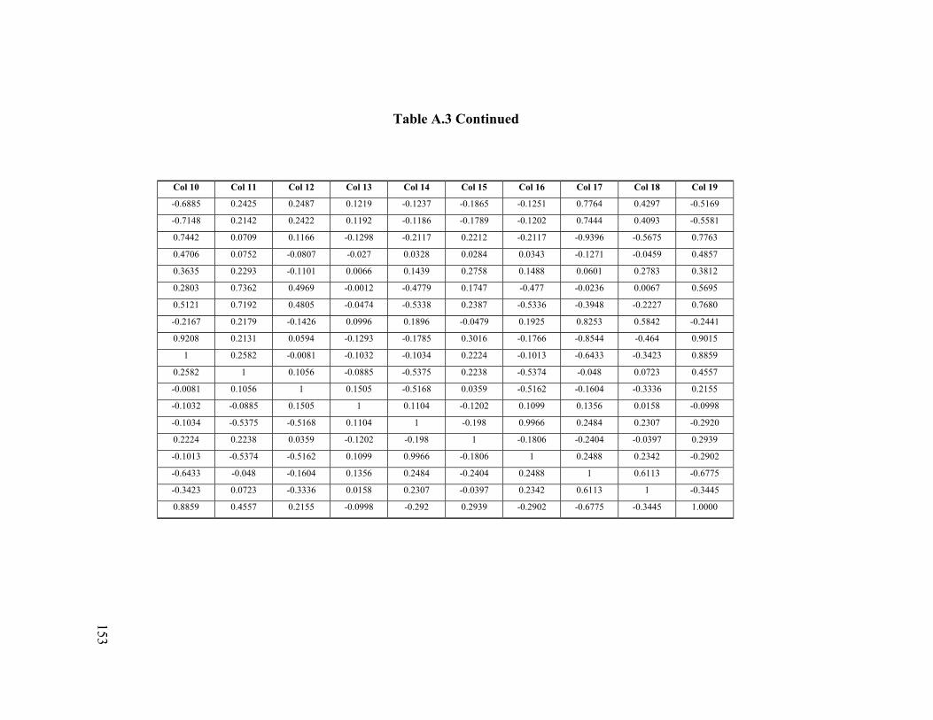
153

Table A.3 Continued

Col 10 Col 11 Col 12 Col 13 Col 14 Col 15 Col 16 Col 17 Col 18 Col 19

-0.6885 0.2425 0.2487 0.1219 -0.1237 -0.1865 -0.1251 0.7764 0.4297 -0.5169

-0.7148 0.2142 0.2422 0.1192 -0.1186 -0.1789 -0.1202 0.7444 0.4093 -0.5581

0.7442 0.0709 0.1166 -0.1298 -0.2117 0.2212 -0.2117 -0.9396 -0.5675 0.7763

0.4706 0.0752 -0.0807 -0.027 0.0328 0.0284 0.0343 -0.1271 -0.0459 0.4857

0.3635 0.2293 -0.1101 0.0066 0.1439 0.2758 0.1488 0.0601 0.2783 0.3812

0.2803 0.7362 0.4969 -0.0012 -0.4779 0.1747 -0.477 -0.0236 0.0067 0.5695

0.5121 0.7192 0.4805 -0.0474 -0.5338 0.2387 -0.5336 -0.3948 -0.2227 0.7680

-0.2167 0.2179 -0.1426 0.0996 0.1896 -0.0479 0.1925 0.8253 0.5842 -0.2441

0.9208 0.2131 0.0594 -0.1293 -0.1785 0.3016 -0.1766 -0.8544 -0.464 0.9015

1 0.2582 -0.0081 -0.1032 -0.1034 0.2224 -0.1013 -0.6433 -0.3423 0.8859

0.2582 1 0.1056 -0.0885 -0.5375 0.2238 -0.5374 -0.048 0.0723 0.4557

-0.0081 0.1056 1 0.1505 -0.5168 0.0359 -0.5162 -0.1604 -0.3336 0.2155

-0.1032 -0.0885 0.1505 1 0.1104 -0.1202 0.1099 0.1356 0.0158 -0.0998

-0.1034 -0.5375 -0.5168 0.1104 1 -0.198 0.9966 0.2484 0.2307 -0.2920

0.2224 0.2238 0.0359 -0.1202 -0.198 1 -0.1806 -0.2404 -0.0397 0.2939

-0.1013 -0.5374 -0.5162 0.1099 0.9966 -0.1806 1 0.2488 0.2342 -0.2902

-0.6433 -0.048 -0.1604 0.1356 0.2484 -0.2404 0.2488 1 0.6113 -0.6775

-0.3423 0.0723 -0.3336 0.0158 0.2307 -0.0397 0.2342 0.6113 1 -0.3445

0.8859 0.4557 0.2155 -0.0998 -0.292 0.2939 -0.2902 -0.6775 -0.3445 1.0000

153

Table A.4 Correlation coefficient Matrix for the Simulated data set Col 1 Col 2 Col 3 Col 4 Col 5 Col 6 Col 7 Col 8 Col 9 Col 10 Col 11 Col 12 Col 13 Col 14

1 0.0142 0.0035 0.0179 0.0037 -0.0005 0.0072 0.1821 0.1813 0.0129 0.0154 0.7137 0.0127 0.0088

0.0142 1 -0.0073 0.0041 0.8535 -0.006 0.0068 0.0502 0.0486 0.8563 0.0033 0.018 0.012 -0.0124

0.0035 -0.0073 1 0.6546 -0.0073 0.6624 0.6615 0.0154 0.0178 -0.0082 0.6694 0.0168 0.6659 0.6689

0.0179 0.0041 0.6546 1 0.0044 0.6543 0.6639 0.0356 0.0376 0.0033 0.6677 0.0331 0.6545 0.6712

0.0037 0.8535 -0.0073 0.0044 1 -0.01 -0.0058 0.0384 0.0361 0.8554 -0.0028 0.0149 0.0109 -0.0155

-0.0005 -0.006 0.6624 0.6543 -0.01 1 0.667 0.0424 0.0468 -0.0069 0.6667 0.0197 0.6673 0.662

0.0072 0.0068 0.6615 0.6639 -0.0058 0.667 1 0.0348 0.0384 -0.001 0.6639 0.0125 0.6665 0.6681

0.1821 0.0502 0.0154 0.0356 0.0384 0.0424 0.0348 1 0.993 0.0367 0.0364 0.1692 0.0245 0.038

0.1813 0.0486 0.0178 0.0376 0.0361 0.0468 0.0384 0.993 1 0.0358 0.0387 0.1697 0.0272 0.0406

0.0129 0.8563 -0.0082 0.0033 0.8554 -0.0069 -0.001 0.0367 0.0358 1 0.0087 0.019 0.0075 -0.0127

0.0154 0.0033 0.6694 0.6677 -0.0028 0.6667 0.6639 0.0364 0.0387 0.0087 1 0.0134 0.6675 0.6713

0.7137 0.018 0.0168 0.0331 0.0149 0.0197 0.0125 0.1692 0.1697 0.019 0.0134 1 0.0223 0.0194

0.0127 0.012 0.6659 0.6545 0.0109 0.6673 0.6665 0.0245 0.0272 0.0075 0.6675 0.0223 1 0.6634

0.0088 -0.0124 0.6689 0.6712 -0.0155 0.662 0.6681 0.038 0.0406 -0.0127 0.6713 0.0194 0.6634 1

0.1833 0.0522 0.018 0.0389 0.0392 0.0466 0.0389 0.993 0.9928 0.0394 0.039 0.1709 0.0274 0.0404

0.704 0.0196 0.0032 0.0049 0.0211 0.0042 0.0016 0.1704 0.1722 0.0159 0.0032 0.7152 0.018 0.0051

0.1801 0.0504 0.0159 0.0383 0.0375 0.044 0.0358 0.9929 0.9931 0.0368 0.0379 0.1672 0.0263 0.038

0.1812 0.0519 0.0183 0.0395 0.0394 0.0467 0.0381 0.9931 0.993 0.039 0.0393 0.1679 0.029 0.0405

0.1801 0.0482 0.0178 0.0401 0.0362 0.0474 0.0387 0.993 0.9931 0.0357 0.0406 0.1675 0.0295 0.0416

0.7102 0.0127 0.0021 0.0037 0.0052 0.0008 -0.0008 0.1744 0.1739 0.0109 0.0033 0.707 0.0014 0.0128

0.1801 0.0499 0.0187 0.0397 0.0373 0.0449 0.0383 0.9929 0.9929 0.0374 0.0386 0.168 0.0285 0.0404

0.0178 -0.0052 0.6654 0.6617 -0.0101 0.6616 0.6656 0.0323 0.0366 -0.0158 0.6728 0.0209 0.6655 0.6738

0.1814 0.0507 0.0173 0.0381 0.0382 0.0438 0.0363 0.993 0.993 0.0386 0.0384 0.1684 0.0259 0.0389

0.1813 0.0492 0.019 0.0391 0.0364 0.0461 0.0374 0.9931 0.993 0.0371 0.0403 0.1691 0.0277 0.0408

0.7068 0.0055 0.016 0.0194 0.0026 0.0094 0.0091 0.156 0.1551 0.0013 0.0125 0.7118 0.0187 0.0182

154

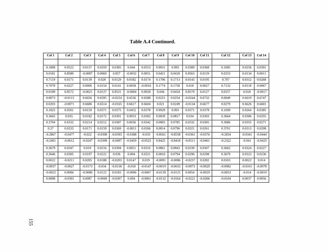
155

Table A.4 Continued.

Col 1 Col 2 Col 3 Col 4 Col 5 Col 6 Col 7 Col 8 Col 9 Col 10 Col 11 Col 12 Col 13 Col 14

0.1808 0.0522 0.0157 0.0359 0.0385 0.044 0.0353 0.9931 0.993 0.0389 0.0368 0.1685 0.0256 0.0391

0.0181 0.8589 -0.0087 0.0069 0.857 -0.0032 0.0051 0.0421 0.0418 0.8563 0.0129 0.0253 0.0134 0.0011

0.7119 0.0171 0.0139 0.028 0.0129 0.0182 0.0174 0.1706 0.1713 0.0143 0.0195 0.707 0.0312 0.0268

0.7078 0.0227 0.0006 0.0154 0.0141 0.0058 -0.0016 0.1774 0.1758 0.018 0.0027 0.7132 0.0118 0.0067

0.0189 0.8572 -0.0021 0.0127 0.8531 -0.0004 0.0028 0.044 0.0434 0.8579 0.0127 0.0257 0.018 -0.0017

0.0073 -0.0115 0.6656 0.6595 -0.0224 0.6536 0.6588 0.0221 0.0254 -0.0244 0.6732 0.0049 0.6619 0.6747

0.0203 -0.0071 0.6686 0.6514 -0.0165 0.6617 0.6604 0.021 0.0249 -0.0134 0.6677 0.0279 0.6626 0.6601

0.1825 0.0501 0.0159 0.0371 0.0375 0.0452 0.0378 0.9929 0.993 0.0371 0.0378 0.1699 0.0264 0.0385

0.3665 0.035 0.0182 0.0172 0.0391 0.0033 0.0302 0.0839 0.0817 0.034 0.0303 0.3664 0.0306 0.0255

0.3704 0.0332 0.0214 0.0212 0.0387 0.0036 0.0342 0.0805 0.0785 0.0332 0.0305 0.3686 0.0355 0.0271

0.37 0.0333 0.0171 0.0159 0.0369 -0.0011 0.0266 0.0814 0.0796 0.0321 0.0261 0.3701 0.0313 0.0208

-0.2867 -0.0477 -0.022 -0.0398 -0.0393 -0.0388 -0.033 -0.8561 -0.8558 -0.0361 -0.0376 -0.2834 -0.0341 -0.0444

-0.2401 -0.0612 -0.0247 -0.0398 -0.0497 -0.0459 -0.0525 0.8425 -0.8418 -0.0511 -0.0461 -0.2322 -0.041 -0.0425

0.3679 0.0347 0.019 0.0216 0.0394 0.0051 0.0316 0.0861 0.0843 0.0339 0.0307 0.3665 0.0324 0.0227

0.3646 0.0305 0.0197 0.0222 0.036 0.004 0.0321 0.0816 0.0794 0.0296 0.0298 0.3679 0.0323 0.0236

0.0022 -0.0211 0.0205 0.0188 -0.0203 0.0147 0.019 -0.0091 -0.0086 -0.0237 0.0282 0.0103 0.0022 0.014

-0.0037 -0.0027 -0.0173 -0.034 -0.0158 -0.018 -0.0147 -0.0019 -0.0033 -0.0073 -0.0029 -0.0082 -0.0101 -0.0078

-0.0022 0.0084 -0.0086 0.0122 0.0183 -0.0096 -0.0067 -0.0139 -0.0125 0.0054 -0.0029 -0.0053 -0.014 -0.0019

0.0008 -0.0301 0.0087 -0.0049 -0.0307 0.004 -0.0061 -0.0132 -0.0164 -0.0221 -0.0206 -0.0104 0.0037 0.0056

155

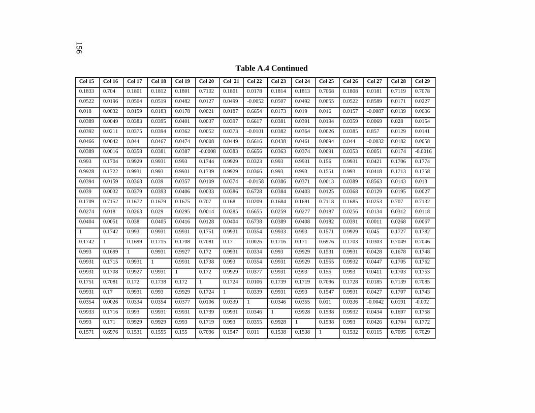
Table A.4 Continued Col 15 Col 16 Col 17 Col 18 Col 19 Col 20 Col 21 Col 22 Col 23 Col 24 Col 25 Col 26 Col 27 Col 28 Col 29

0.1833 0.704 0.1801 0.1812 0.1801 0.7102 0.1801 0.0178 0.1814 0.1813 0.7068 0.1808 0.0181 0.7119 0.7078

0.0522 0.0196 0.0504 0.0519 0.0482 0.0127 0.0499 -0.0052 0.0507 0.0492 0.0055 0.0522 0.8589 0.0171 0.0227

0.018 0.0032 0.0159 0.0183 0.0178 0.0021 0.0187 0.6654 0.0173 0.019 0.016 0.0157 -0.0087 0.0139 0.0006

0.0389 0.0049 0.0383 0.0395 0.0401 0.0037 0.0397 0.6617 0.0381 0.0391 0.0194 0.0359 0.0069 0.028 0.0154

0.0392 0.0211 0.0375 0.0394 0.0362 0.0052 0.0373 -0.0101 0.0382 0.0364 0.0026 0.0385 0.857 0.0129 0.0141

0.0466 0.0042 0.044 0.0467 0.0474 0.0008 0.0449 0.6616 0.0438 0.0461 0.0094 0.044 -0.0032 0.0182 0.0058

0.0389 0.0016 0.0358 0.0381 0.0387 -0.0008 0.0383 0.6656 0.0363 0.0374 0.0091 0.0353 0.0051 0.0174 -0.0016

0.993 0.1704 0.9929 0.9931 0.993 0.1744 0.9929 0.0323 0.993 0.9931 0.156 0.9931 0.0421 0.1706 0.1774

0.9928 0.1722 0.9931 0.993 0.9931 0.1739 0.9929 0.0366 0.993 0.993 0.1551 0.993 0.0418 0.1713 0.1758

0.0394 0.0159 0.0368 0.039 0.0357 0.0109 0.0374 -0.0158 0.0386 0.0371 0.0013 0.0389 0.8563 0.0143 0.018

0.039 0.0032 0.0379 0.0393 0.0406 0.0033 0.0386 0.6728 0.0384 0.0403 0.0125 0.0368 0.0129 0.0195 0.0027

0.1709 0.7152 0.1672 0.1679 0.1675 0.707 0.168 0.0209 0.1684 0.1691 0.7118 0.1685 0.0253 0.707 0.7132

0.0274 0.018 0.0263 0.029 0.0295 0.0014 0.0285 0.6655 0.0259 0.0277 0.0187 0.0256 0.0134 0.0312 0.0118

0.0404 0.0051 0.038 0.0405 0.0416 0.0128 0.0404 0.6738 0.0389 0.0408 0.0182 0.0391 0.0011 0.0268 0.0067

1 0.1742 0.993 0.9931 0.9931 0.1751 0.9931 0.0354 0.9933 0.993 0.1571 0.9929 0.045 0.1727 0.1782

0.1742 1 0.1699 0.1715 0.1708 0.7081 0.17 0.0026 0.1716 0.171 0.6976 0.1703 0.0303 0.7049 0.7046

0.993 0.1699 1 0.9931 0.9927 0.172 0.9931 0.0334 0.993 0.9929 0.1531 0.9931 0.0428 0.1678 0.1748

0.9931 0.1715 0.9931 1 0.9931 0.1738 0.993 0.0354 0.9931 0.9929 0.1555 0.9932 0.0447 0.1705 0.1762

0.9931 0.1708 0.9927 0.9931 1 0.172 0.9929 0.0377 0.9931 0.993 0.155 0.993 0.0411 0.1703 0.1753

0.1751 0.7081 0.172 0.1738 0.172 1 0.1724 0.0106 0.1739 0.1719 0.7096 0.1728 0.0185 0.7139 0.7085

0.9931 0.17 0.9931 0.993 0.9929 0.1724 1 0.0339 0.9931 0.993 0.1547 0.9931 0.0427 0.1707 0.1743

0.0354 0.0026 0.0334 0.0354 0.0377 0.0106 0.0339 1 0.0346 0.0355 0.011 0.0336 -0.0042 0.0191 -0.002

0.9933 0.1716 0.993 0.9931 0.9931 0.1739 0.9931 0.0346 1 0.9928 0.1538 0.9932 0.0434 0.1697 0.1758

0.993 0.171 0.9929 0.9929 0.993 0.1719 0.993 0.0355 0.9928 1 0.1538 0.993 0.0426 0.1704 0.1772

0.1571 0.6976 0.1531 0.1555 0.155 0.7096 0.1547 0.011 0.1538 0.1538 1 0.1532 0.0115 0.7095 0.7029

156

157

Table A.4 Continued

Col 15 Col 16 Col 17 Col 18 Col 19 Col 20 Col 21 Col 22 Col 23 Col 24 Col 25 Col 26 Col 27 Col 28 Col 29

0.9929 0.1703 0.9931 0.9932 0.993 0.1728 0.9931 0.0336 0.9932 0.993 0.1532 1 0.0445 0.1695 0.1759

0.045 0.0303 0.0428 0.0447 0.0411 0.0185 0.0427 -0.0042 0.0434 0.0426 0.0115 0.0445 1 0.021 0.0244

0.1727 0.7049 0.1678 0.1705 0.1703 0.7139 0.1707 0.0191 0.1697 0.1704 0.7095 0.1695 0.021 1 0.7065

0.1782 0.7046 0.1748 0.1762 0.1753 0.7085 0.1743 -0.002 0.1758 0.1772 0.7029 0.1759 0.0244 0.7065 1

0.0469 0.0305 0.0448 0.047 0.0435 0.0196 0.0443 -0.0082 0.0456 0.0442 0.0113 0.0471 0.8575 0 .0282 0.0225

0.024 -0.0041 0.0233 0.0252 0.0254 -0.01 0.0248 0.6575 0.0241 0.026 -0.0022 0.0219 -0.0064 0.0143 -0.0139

0.0255 0.0091 0.0239 0.0251 0.0258 0.0109 0.0245 0.658 0.0233 0.0253 0.0238 0.0228 -0.0084 0.0302 -0.0044

0.9928 0.1725 0.9929 0.9932 0.9928 0.174 0.9929 0.0335 0.993 0.9928 0.1563 0.993 0.0418 0.1709 0.1784

0.0842 0.3608 0.0844 0.082 0.0836 0.3648 0.083 0.0203 0.0822 0.0817 0.3679 0.082 0.0437 0.3742 0.3728

0.0809 0.364 0.0808 0.0787 0.0799 0.3666 0.0799 0.0251 0.0787 0.0782 0.3695 0.0785 0.0447 0.3769 0.3737

0.0816 0.3617 0.0817 0.0795 0.0805 0.3672 0.08 0.0188 0.0794 0.0793 0.3684 0.0795 0.0428 0.3725 0.3729

-0.8574 -0.2828 -0.8563 -0.8568 -0.8564 -0.2789 -0.8561 -0.0396 -0.856 -0.8559 -0.2767 -0.8565 -0.0427 -0.2793 -0.2836

-0.8423 -0.2332 -0.8426 -0.8412 -0.8415 -0.2339 -0.842 -0.0418 -0.8421 -0.8422 -0.2163 -0.8414 -0.0636 -0.2346 -0.2362

0.0863 0.3587 0.0866 0.0843 0.0856 0.3645 0.0851 0.0218 0.0844 0.0844 0.3658 0.0844 0.0442 0.3737 0.3715

0.0819 0.3588 0.0816 0.0799 0.0809 0.3654 0.0808 0.022 0.0797 0.08 0.3681 0.0797 0.0415 0.3725 0.3715

-0.0068 -0.001 -0.0099 -0.0073 -0.0095 0.0038 -0.008 0.0128 -0.0077 -0.0064 0.0074 -0.0069 -0.023 0.0071 0.0118

-0.0022 0.0059 -0.0046 -0.0026 -0.0014 0.0017 -0.002 -0.0177 -0.0025 -0.0026 0.0035 -0.0008 -0.0048 -0.0066 -0.016

-0.0155 -0.0066 -0.0107 -0.0165 -0.014 0.0033 -0.0173 -0.0072 -0.0139 -0.015 -0.0187 -0.0124 0.0071 -0.0109 0.0031

-0.0124 -0.0118 -0.0147 -0.0149 -0.0135 0.0081 -0.016 0.0012 -0.0171 -0.0148 -0.01 -0.0169 -0.0298 -0.0149 0.0023

0.0189 0.0073 0.0203 0.1825 0.3665 0.3704 0.37 -0.2867 -0.2401 0.3679 0.3646 0.0022 -0.0037 -0.0022 0.0008

0.8572 -0.0115 -0.0071 0.0501 0.035 0.0332 0.0333 -0.0477 -0.0612 0.0347 0.0305 -0.0211 -0.0027 0.0084 -0.0301

157

158

Table A.4 Continued Col 30 Col 31 Col 32 Col 33 Col 34 Col 35 Col 36 Col 37 Col 38 Col 39 Col 40 Col 41 Col 42 Col 43 Col 44

-0.0021 0.6656 0.6686 0.0159 0.0182 0.0214 0.0171 -0.022 -0.0247 0.019 0.0197 0.0205 -0.0173 -0.0086 0.0087

0.0127 0.6595 0.6514 0.0371 0.0172 0.0212 0.0159 -0.0398 -0.0398 0.0216 0.0222 0.0188 -0.034 0.0122 -0.0049

0.8531 -0.0224 -0.0165 0.0375 0.0391 0.0387 0.0369 -0.0393 -0.0497 0.0394 0.036 -0.0203 -0.0158 0.0183 -0.0307

-0.0004 0.6536 0.6617 0.0452 0.0033 0.0036 -0.0011 -0.0388 -0.0459 0.0051 0.004 0.0147 -0.018 -0.0096 0.004

0.0028 0.6588 0.6604 0.0378 0.0302 0.0342 0.0266 -0.033 -0.0525 0.0316 0.0321 0.019 -0.0147 -0.0067 -0.0061

0.044 0.0221 0.021 0.9929 0.0839 0.0805 0.0814 -0.8561 -0.8425 0.0861 0.0816 -0.0091 -0.0019 -0.0139 -0.0132

0.0434 0.0254 0.0249 0.993 0.0817 0.0785 0.0796 -0.8558 -0.8418 0.0843 0.0794 -0.0086 -0.0033 -0.0125 -0.0164

0.8579 -0.0244 -0.0134 0.0371 0.034 0.0332 0.0321 -0.0361 -0.0511 0.0339 0.0296 -0.0237 -0.0073 0.0054 -0.0221

0.0127 0.6732 0.6677 0.0378 0.0303 0.0305 0.0261 -0.0376 -0.0461 0.0307 0.0298 0.0282 -0.0029 -0.0029 -0.0206

0.0257 0.0049 0.0279 0.1699 0.3664 0.3686 0.3701 -0.2834 -0.2322 0.3665 0.3679 0.0103 -0.0082 -0.0053 -0.0104

0.018 0.6619 0.6626 0.0264 0.0306 0.0355 0.0313 -0.0341 -0.041 0.0324 0.0323 0.0022 -0.0101 -0.014 0.0037

-0.0017 0.6747 0.6601 0.0385 0.0255 0.0271 0.0208 -0.0444 -0.0425 0.0227 0.0236 0.014 -0.0078 -0.0019 0.0056

0.0469 0.024 0.0255 0.9928 0.0842 0.0809 0.0816 -0.8574 -0.8423 0.0863 0.0819 -0.0068 -0.0022 -0.0155 -0.0124

0.0305 -0.0041 0.0091 0.1725 0.3608 0.364 0.3617 -0.2828 -0.2332 0.3587 0.3588 -0.001 0.0059 -0.0066 -0.0118

0.0448 0.0233 0.0239 0.9929 0.0844 0.0808 0.0817 -0.8563 -0.8426 0.0866 0.0816 -0.0099 -0.0046 -0.0107 -0.0147

0.047 0.0252 0.0251 0.9932 0.082 0.0787 0.0795 -0.8568 -0.8412 0.0843 0.0799 -0.0073 -0.0026 -0.0165 -0.0149

0.0435 0.0254 0.0258 0.9928 0.0836 0.0799 0.0805 -0.8564 -0.8415 0.0856 0.0809 -0.0095 -0.0014 -0.014 -0.0135

0.0196 -0.01 0.0109 0.174 0.3648 0.3666 0.3672 -0.2789 -0.2339 0.3645 0.3654 0.0038 0.0017 0.0033 0.0081

0.0443 0.0248 0.0245 0.9929 0.083 0.0799 0.08 -0.8561 -0.842 0.0851 0.0808 -0.008 -0.002 -0.0173 -0.016

-0.0082 0.6575 0.658 0.0335 0.0203 0.0251 0.0188 -0.0396 -0.0418 0.0218 0.022 0.0128 -0.0177 -0.0072 0.0012

0.0456 0.0241 0.0233 0.993 0.0822 0.0787 0.0794 -0.856 -0.8421 0.0844 0.0797 -0.0077 -0.0025 -0.0139 -0.0171

0.0442 0.026 0.0253 0.9928 0.0817 0.0782 0.0793 -0.8559 -0.8422 0.0844 0.08 -0.0064 -0.0026 -0.015 -0.0148

0.0113 -0.0022 0.0238 0.1563 0.3679 0.3695 0.3684 -0.2767 -0.2163 0.3658 0.3681 0.0074 0.0035 -0.0187 -0.01

0.0471 0.0219 0.0228 0.993 0.082 0.0785 0.0795 -0.8565 -0.8414 0.0844 0.0797 -0.0069 -0.0008 -0.0124 -0.0169

0.8575 -0.0064 -0.0084 0.0418 0.0437 0.0447 0.0428 -0.0427 -00636 0.0442 0.0415 -0.023 -0.0048 0.0071 -0.0298

0.0282 0.0143 0.0302 0.1709 0 3742 0.3769 0.3725 -0.2793 -0.2346 0.3737 0.3725 0.0071 -0.0066 -0.0109 -0.0149

158

159

Table A.4 Continued

Col 30 Col 31 Col 32 Col 33 Col 34 Col 35 Col 36 Col 37 Col 38 Col 39 Col 40 Col 41 Col 42 Col 43 Col 44

0.0225 -0.0139 -0.0044 0.1784 0 3728 0.3737 0.3729 -0.2836 -0.2362 0.3715 0.3715 0.0118 -0.016 0.0031 0.0023

1 -0.0035 -0.0055 0.0443 0.0409 0.0396 0.0386 -0.0391 -0.0638 0.0396 0.0367 -0.0288 -0.0079 0.0184 -0.0262

-0.0035 1 0.6686 0.0236 0.0181 0.0213 0.0191 -0.0233 -0.0344 0.0196 0.0226 0.02 -0.0006 -0.0039 0.0142

-0.0055 0.6686 1 0.0235 0.0266 0.0301 0.0264 -0.0276 -0.0337 0.026 0.0293 0.0216 -0.0161 0.0022 0.0019

0.0443 0.0236 0.0235 1 0.0823 0.0792 0.0796 -0.8565 -0.8412 0.0844 0.0803 -0.0067 -0.004 -0.0141 -0.0168

0.0409 0.0181 0.0266 0.0823 1 0.9765 0.9764 -0.2673 -0.4005 0.9761 0.9766 -0.0008 0.0183 0.0194 -0.0111

0.0396 0.0213 0.0301 0.0792 0.9765 1 0.9764 -0.2637 -0.3985 0.9763 0.9764 -0.0025 0.0116 0.0119 -0.0139

0.0386 0.0191 0.0264 0.0796 0.9764 0.9764 1 -0.2637 -0.3993 0.9768 0.9767 -0.0033 0.0137 0.0123 -0.0137

-0.0391 -0.0233 -0.0276 -0.8565 -0. 2673 -0.2637 -0.2637 1 0.6577 -0.267 -0.2651 0.0072 -0.0022 0.0102 0.0164

-0.0638 -0.0344 -0.0337 -0.8412 -0.4005 -0.3985 -0.3993 0.6577 1 -0.4038 -0.3987 0.0076 0.0012 0.0053 0.013

0.0396 0.0196 0.026 0.0844 0.9761 0.9763 0.9768 -0.267 -0.4038 1 0.9764 -0.006 0.0168 0.0159 -0.0122

0.0367 0.0226 0.0293 0.0803 0.9766 0.9764 0.9767 -0.2651 -0.3987 0.9764 1 0.0003 0.0172 0.0103 -0.0143

-0.0288 0.02 0.0216 -0.0067 -0.0008 -0.0025 -0.0033 0.0072 0.0076 -0.006 0.0003 1 -0.0155 -0.0175 -0.012

-0.0079 -0.0006 -0.0161 -0.004 0.0183 0.0116 0.0137 -0.0022 0.0012 0.0168 0.0172 -0.0155 1 -0.0091 0.0185

0.0184 -0.0039 0.0022 -0.0141 0.0194 0.0119 0.0123 0.0102 0.0053 0.0159 0.0103 -0.0175 -0.0091 1 0.0004

-0.0262 0.0142 0.0019 -0.0168 -0.0111 -0.0139 -0.0137 0.0164 0.013 -0.0122 -0.0143 -0.012 0.0185 0.0004 1

159

160

Table A.5 Malinowski's eigenvalues for the Boston Housing Data.

Factors Reduced eigenvalues

1 0.4441

2 0.0295

3 0.0020

4 0.0014

5 0.0007

6 0.0001

7 0.0001

8 0.0001

9 0.0000

10 0.0000

11 0.0000

12 0.0000

13 0.0000

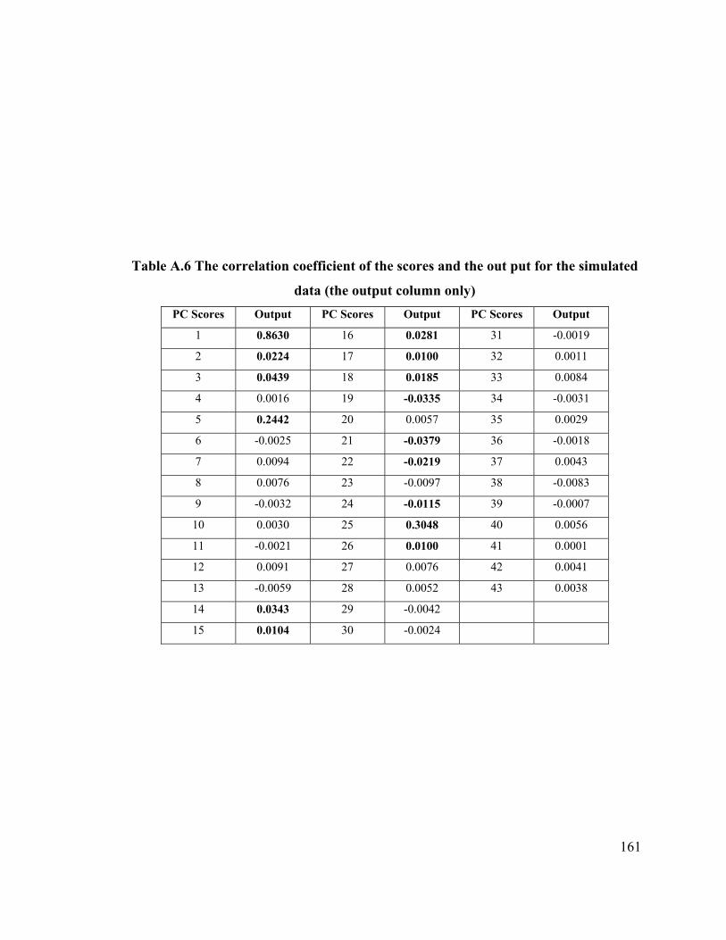
161

Table A.6 The correlation coefficient of the scores and the out put for the simulated

data (the output column only) PC Scores Output PC Scores Output PC Scores Output

1 0.8630 16 0.0281 31 -0.0019

2 0.0224 17 0.0100 32 0.0011

3 0.0439 18 0.0185 33 0.0084

4 0.0016 19 -0.0335 34 -0.0031

5 0.2442 20 0.0057 35 0.0029

6 -0.0025 21 -0.0379 36 -0.0018

7 0.0094 22 -0.0219 37 0.0043

8 0.0076 23 -0.0097 38 -0.0083

9 -0.0032 24 -0.0115 39 -0.0007

10 0.0030 25 0.3048 40 0.0056

11 -0.0021 26 0.0100 41 0.0001

12 0.0091 27 0.0076 42 0.0041

13 -0.0059 28 0.0052 43 0.0038

14 0.0343 29 -0.0042

15 0.0104 30 -0.0024

162

Table A.7. Boston Housing Data Set CRIM ZN IND. CHAS NOX RMS AGE DIST RAD TAX PT B LSTAT MVAL

1 0.00632 18 2.31 0 0.538 6.575 65.2 4.09 1 296 15.3 396.9 4.98 24

2 0.02731 0 7.07 0 0.469 6.421 78.9 4.9671 2 242 17.8 396.9 9.14 21.6

3 0.02729 0 7.07 0 0.469 7.185 61.1 4.9671 2 242 17.8 392.83 4.03 34.7

4 0.03237 0 2.18 0 0.458 6.998 45.8 6.0622 3 222 18.7 394.63 2.94 33.4

5 0.06905 0 2.18 0 0.458 7.147 54.2 6.0622 3 222 18.7 396.9 5.33 36.2

6 0.02985 0 2.18 0 0.458 6.43 58.7 6.0622 3 222 18.7 394.12 5.21 28.7

7 0.08829 12.5 7.87 0 0.524 6.012 66.6 5.5605 5 311 15.2 395.6 12.43 22.9

8 0.14455 12.5 7.87 0 0.524 6.172 96.1 5.9505 5 311 15.2 396.9 19.15 27.1

9 0.21124 12.5 7.87 0 0.524 5.631 100 6.0821 5 311 15.2 386.63 29.93 16.5

10 0.17004 12.5 7.87 0 0.524 6.004 85.9 6.5921 5 311 15.2 386.71 17.1 18.9

11 0.22489 12.5 7.87 0 0.524 6.377 94.3 6.3467 5 311 15.2 392.52 20.45 15

12 0.11747 12.5 7.87 0 0.524 6.009 82.9 6.2267 5 311 15.2 396.9 13.27 18.9

13 0.09378 12.5 7.87 0 0.524 5.889 39 5.4509 5 311 15.2 390.5 15.71 21.7

14 0.62976 0 8.14 0 0.538 5.949 61.8 4.7075 4 307 21 396.9 8.26 20.4

15 0.63796 0 8.14 0 0.538 6.096 84.5 4.4619 4 307 21 380.02 10.26 18.2

16 0.62739 0 8.14 0 0.538 5.834 56.5 4.4986 4 307 21 395.62 8.47 19.9

17 1.05393 0 8.14 0 0.538 5.935 29.3 4.4986 4 307 21 386.85 6.58 23.1

18 0.7842 0 8.14 0 0.538 5.99 81.7 4.2579 4 307 21 386.75 14.67 17.5

19 0.80271 0 8.14 0 0.538 5.456 36.6 3.7965 4 307 21 288.99 11.69 20.2

20 0.7258 0 8.14 0 0.538 5.727 69.5 3.7965 4 307 21 390.95 11.28 18.2

21 1.25179 0 8.14 0 0.538 5.57 98.1 3.7979 4 307 21 376.57 21.02 13.6

22 0.85204 0 8.14 0 0.538 5.965 89.2 4.0123 4 307 21 392.53 13.83 19.6

23 1.23247 0 8.14 0 0.538 6.142 91.7 3.9769 4 307 21 396.9 18.72 15.2

24 0.98843 0 8.14 0 0.538 5.813 100 4.0952 4 307 21 394.54 19.88 14.5

25 0.75026 0 8.14 0 0.538 5.924 94.1 4.3996 4 307 21 394.33 16.3 15.6

26 0.84054 0 8.14 0 0.538 5.599 85.7 4.4546 4 307 21 303.42 16.51 13.9

27 0.67191 0 8.14 0 0.538 5.813 90.3 4.682 4 307 21 376.88 14.81 16.6

28 0.95577 0 8.14 0 0.538 6.047 88.8 4.4534 4 307 21 306.38 17.28 14.8

29 0.77299 0 8.14 0 0.538 6.495 94.4 4.4547 4 307 21 387.94 12.8 18.4

30 1.00245 0 8.14 0 0.538 6.674 87.3 4.239 4 307 21 380.23 11.98 21

31 1.13081 0 8.14 0 0.538 5.713 94.1 4.233 4 307 21 360.17 22.6 12.7

32 1.35472 0 8.14 0 0.538 6.072 100 4.175 4 307 21 376.73 13.04 14.5

33 1.38799 0 8.14 0 0.538 5.95 82 3.99 4 307 21 232.6 27.71 13.2

34 1.15172 0 8.14 0 0.538 5.701 95 3.7872 4 307 21 358.77 18.35 13.1

35 1.61282 0 8.14 0 0.538 6.096 96.9 3.7598 4 307 21 248.31 20.34 13.5

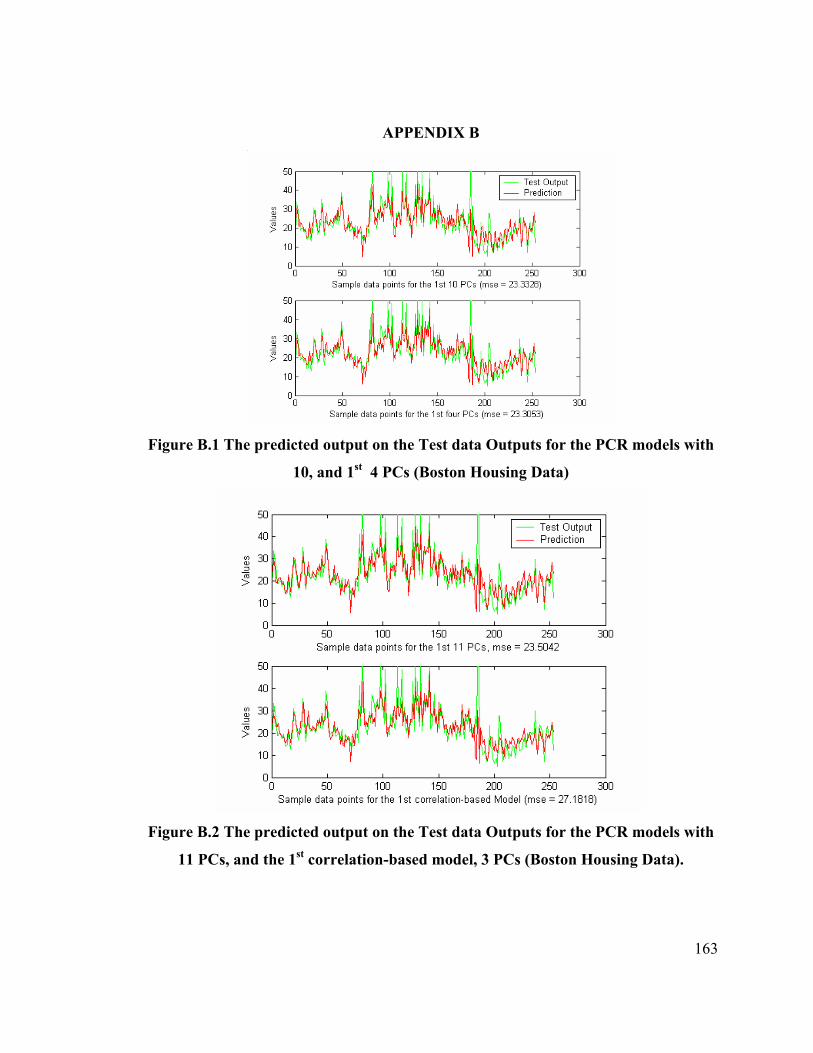
163

APPENDIX B

Figure B.1 The predicted output on the Test data Outputs for the PCR models with

10, and 1st 4 PCs (Boston Housing Data)

Figure B.2 The predicted output on the Test data Outputs for the PCR models with

11 PCs, and the 1st correlation-based model, 3 PCs (Boston Housing Data).

164

APPENDIX C THE MATLAB CODES

165

%Boston Housing data set %http://lib.stat.cmu.edu/datasets/ load boston_data x = Sheet3; [m n] = size(x); X= x(:,1:n-1); Y = x(:,n); % %The Airliner data set. % load airliner_data % x = airliner_data; % [m n] = size(x); % X = x(:,1:n-1); % Y = x(:,n); % load col_data % [m n] = size(x); %load sim %the simulated data set %x = Data; %[m n] = size(x); %X = x(:,[1:37 39:n]); %Y = x(:,38); x1 = [x y]; % concatenating the output and input variables %Division of the data set into training and test set N = size(x1,1); j = 1; step = 200; %test for excess rows left = rem(N, 2*step); num_times = fix(N/(2*step)); ntimes = 1; for i = 1:2*step:N tr_data(j:j+(step - 1),:) = x1(i:i + (step - 1),:); te_data(j:j+(step - 1),:) = x1(i+step: i + (2*step - 1), :); if (ntimes == num_times) break; end

166

j = j + step; ntimes = ntimes + 1; end xytrn = [tr_data' (x1([9201:9350 9501:9593],:))']'; xxtest = [te_data' (x1(9351:9500,:))']'; %xytrn = [tr_data' (x1(9593,:))']'; %redistribute those left --- the number of rows left is stored in the %variable "left" % num_rows = num_times*step + left % seperating the x and y matrix train_data_x1 = xytrn(:,1:7); train_data_y = xytrn(:,8); test_data_x1 =xxtest(:,1:7); test_data_y = xxtest(:,8); train_data_x = [ones(size(train_data_x1,1),1) train_data_x1]; test_data_x = [ones(size(test_data_x1,1),1) test_data_x1]; condtn = cond(train_data_x1'*train_data_x1); [m1 n1] = size(train_data_x1) % size of data before appending column of ones [m n] = size(train_data_x); % size of data after appending column of ones %Ordinary Least Square or Multiple Linear Regression BM1 = regress(train_data_y,train_data_x) NB1 = norm(BM1); train_yhat = train_data_x*BM1; test_yhat = test_data_x*BM1; %Statistics for model evaluation errtr = (train_data_y - train_yhat);%error training data errts = (test_data_y -test_yhat); %error test data msetr = mean(errtr.^2); %mean square error training % msq_err_tr= mean((train_data_y - (train_yhat)).^2) %train case msets = mean(errts.^2); % mean sq.error test data rmsets = sqrt(msets); % root mean square error % msq_err_ts= mean((test_data_y - (test_yhat )).^2) %test case maets = mean(abs(errts)); % mean absolute error test data sse = sum(errts.^2); % sum of square error ave_y = mean(test_data_y); % ssr = sum((test_yhat - ave_y).^2); %sum of square error regression ssto = sum((test_data_y - ave_y).^2); ssre = ssto - sse;

167

savr = sum(abs(test_yhat - ave_y)); % sum of absolute value regression % sst = sse + ssr; %total sum of square error rsq = ssre/ssto; % rsq = 1-sse/sst R-SQUARE rsqr= 1 - (sse/ssto); df = m-1; p = n; ast = ssto/df rsq_adj = 1 - (df/(m-p))*sse/ssto; %R-Square Adjusted rsq_adj1 = 1- (msets/ast); saverr = sum(abs(errts)); Mod_E = 1 - (saverr/savr); %Modified coefficient of efficiency % display results tc = [rsq;rsq_adj;msets;rmsets;maets;Mod_E]'; fprintf('Statistics for model Evaluation\n') fprintf(' rsq; rsq_adj; msets; rmsets; maets; Mod_E\n') fprintf('-------------------------------------------------------------------\n') disp([tc])% to create a matrix of 5 rows disp(condtn) disp(NB1) disp(BM1) %By Godswill Nsofor %University of Tennessee, Knoxville %Department of Industrial Engineering %May 2006 %Using correlation coefficient to build the model CC = corrcoef(xytrn); disp(CC(:,n)) disp(CC(1:5,1:5)) % show a few of the correlation coefficient matrix tdx = train_data_x(:,1:n); % train data with the variables most correlated to the output variable, %with column of ones tsdx = test_data_x(:,1:n); % the test data having variables correlated with the output %variable, with column of ones [m n] = size(tsdx); BM2 = regress(train_data_y,tdx); yhat_tr = (tdx*BM2); mserr_tr = mean((train_data_y - yhat_tr).^2) %error of training case yhat_ts =(tsdx*BM2); %The Stepwise regression approach tdx1 = train_data_x(:,[2:n]); % removing the ones column since the software will scale the data % [m p] = size(tdx1)

168

% alfa = 1 - (1 - 0.025).^(1/p) %95% confidence interval stepwise(tdx1,train_data_y); tdx3 = train_data_x(:,1:n); % significant columns added tsdtx3 = test_data_x(:,1:n); [m n] = size(tsdtx3); BM3 = regress(train_data_y,tdx3); yhat_trr = (tdx3*BM3); yhat_tss = (tsdtx3*BM3); NB3 = norm(BM3); % the norm or weight of the regression coefficients condt3 = cond(tdx3'*tdx3); %condition number of the matrix figure(1) plot(test_data_y,'g');hold on; plot(test_yhat,'r');hold off; xlabel('A. All the Input Variables') title('The Predicted Outputs against the Test data Output') legend('Test Output','Prediction') %PCR %scaling the data matrix% [Xtrn1, meanval, stdval]=zscore1(train_data_x1); %scoring of the data sets [Xtest1, meanval, stdval]=zscore1(test_data_x1, meanval, stdval); [Ytrn1, meanvaly, stdvaly]=zscore1(train_data_y); [Ytest1, meanvaly, stdvaly]=zscore1(test_data_y, meanvaly, stdvaly); %Siingular Value Decomposition [U S V] = svd(Xtrn1,0); [PC LAT EXP] = pcacov(Xtrn1); [l w] = size(S); condition_number = (S(1,1)^2)/(S(l,w)^2); % Loadings plots of the pcs figure(10) subplot(4,2,1), bar(PC(:,1),0.5) title('Loadings 1 vs index#') grid on subplot(4,2,2), bar(PC(:,2),0.5) title('Loadings 2 vs index#') grid on subplot(4,2,3), bar(PC(:,3),0.5) title('Loadings 3 vs index#') grid on subplot(4,2,4), bar(PC(:,4),0.5)

169

title('Loadings 4 vs index#') grid on %Percentage Variation in the pcs figure(12) subplot(2,1,1), plot(LAT) xlabel('Number of PCs') ylabel('Eigenvalues') title('Eigenvalues vs PCs') grid on cs = cumsum(EXP); subplot(2,1,2), plot(cs) xlabel('number of PCs'); ylabel('% information explained'); title('Cumulative % information explained in the PCs'); grid on %Knee in the Latent or Eigen values plot. k = n; %number of pcs in the first knee Z = U*S; %score matrix z = Z(:,1:k); % picking the first ten PCs and the rest are regarded as noise. %Regress with the selected PCs Bpc1 = regress(Ytrn1,z); yhat_trpc1 = z*Bpc1; %train data prediction yhattrpc1 = unscore(yhat_trpc1,meanvaly,stdvaly); %unscoring %test data case ztest = Xtest1*V; %score matrix ztest1 = ztest(:,1:k); [m n] = size(ztest1); yhat_tspc1 = ztest1*Bpc1; %test data prediction yhattspc1 = unscore(yhat_tspc1,meanvaly,stdvaly); %unscoring %ridge regression Sv = svd(Xtrn1); %singular value decomposition condition_number = (S(1,1)^2)/(S(l,w)^2); %same as condition # = cond(Xtrn1'*Xtrn1) % ordinary Ridge regression (FULL MODEL) with standardized data. BR2 = ridge(Ytrn1,Xtrn1,0); NBR2 = norm(BR2); train_yhatR2 = Xtrn1*BR2; yhattrR2 = unscore(train_yhatR2,meanvaly,stdvaly); %training prediction

170

test_yhatR2 = Xtest1*BR2; % test set prediction yhattsR2 = unscore(test_yhatR2,meanvaly,stdvaly); %Ridge using reguarization parameter alpha %Cross validation Sv = svd(Xtrn1); %singular values (ranged from 4 to 40, between 10^0 and 10^2) %let alpha cross validation be alpha_cv alpha_cv = logspace(0.5,3.5,80); % alpha_cv in the range of the singular values MSE_r = zeros(1,80); noRmb = zeros(1,80); con_r = zeros(1,80); for i = 1:80 BR3 = ridge(Ytrn1,Xtrn1,alpha_cv(i)^2); %Using each alpha value noRmb(i) = norm(BR3); ypr =Xtest1*BR3; yhattestR3 = unscore(ypr,meanvaly,stdvaly); error_R3 = yhattestR3 - test_data_y; MSE_r(i) = mean(error_R3.^2); e2 =eig(Xtrn1'*Xtrn1 + alpha_cv(i)^2*eye(size(Xtrn1,2))); con_r(i) = max(e2)/min(e2); end figure(30) semilogx(alpha_cv,MSE_r) title('Error versus Alpha'); xlabel('Regularization Coefficient: Alpha'); ylabel('Mean Squared Error'); grid on ind3 = find(min(MSE_r)==MSE_r) Min_mse = [MSE_r(ind3) min(MSE_r)] tt3 = alpha_cv(ind3) NBX3 = noRmb(ind3) cn3 = con_r(ind3) %showing the relationship between Alpha and condition # figure(31) plot(con_r,alpha_cv) xlabel('condition number'); ylabel('alpha') title('Plot of condition number versus alpha') %showing the relationship between the weights and alpha figure(32)

171

semilogx(alpha_cv,noRmb) title('Weights Size versus Alpha'); xlabel('Regularization Coefficients: Alpha'); ylabel('Norm(BR)') grid on % the main L-Curve figure(33) plot(MSE_r,noRmb) title('Weight size versus Average Error'); xlabel('Mean Squared Error'); ylabel('Norm(BR3)') grid on ind2 = find(min(abs(noRmb-0.7)==abs(noRmb-0.7)) Min_mse = [MSE_r(ind2) min(MSE_r)] alph2 = alpha_cv(ind2); % Min_Errorr = min(MSE_r); wt = noRmb(ind2); CN = con_r(ind2); % the condition number is reduced drastically initial_condtn_r = cond(Xtrn1'*Xtrn1); disp([alph2 Min_mse(1) wt CN]) %PLS [p,q,w,b,t,u,e,f,s] = pls(Xtrn1,Ytrn1); %pls in latent variables [34] [reig]=red_eig(Xtrn1, p, q, w, b);%Malinowski's reduced eigenvalues disp(reig') figure(40) plot(reig) %plot of the reduced eigenvalues title('Plot of Reduced Eigenvalues'); xlabel('Index');ylabel('Reduced Eigenvalues'); [Ytrnp]=plspred(Xtrn1,p,q,w,b,n); yptrn=unscore(Ytrnp,meanvaly,stdvaly); % prediction on the test data [Ytestp]=plspred(Xtest1,p,q,w,b,n); % n = # of factors yptestPLS1=unscore(Ytestp,meanvaly,stdvaly); % sq_err_tsPLS1=(test_data_y - yptestPLS1).^2; % computing the error % ave_error2 = mean(sq_err_tsPLS1) %iterative process of finding optimal factors MSE1=zeros(1,13);

172

for i = 1:13 [Y1] = plspred(Xtest1,p,q,w,b,i); %[Ytestp] = plspred(Xtest1,p,q,w,b,n); % n = # of factors [yptest1] = unscore(Y1,meanvaly,stdvaly); serr_ts = (test_data_y - yptest1).^2; MSE1(i) = mean(serr_ts); end figure(44) plot(MSE1); xlabel('Latent Factors Used'); ylabel('Mean Squared Error') title('The plot of the Latent factors and the MSE') indpls = find(min(MSE1)==MSE1) n = indpls % picking optimal number of factors [Ytestp]=plspred(Xtest1,p,q,w,b,indpls); yptestPLS2=unscore(Ytestp,meanvaly,stdvaly); %Check the t and u, inner and outer scores for any non-linear relationship [p,q,w,b,T,U,X,Y]=pls(Xtrn1,Ytrn1); figure(49) yest=b(1)*T(:,1); % plot(T(:,1),U(:,1),'g+'); hold on % matrix of input scores and output scores respectively % plot(T(:,1),yest,'r*'); hold off % matrix of output scores and predicted yest % title('Internal scores vs the predicted internal scores') % legend('Scores','Prediction') yest2=b(2)*T(:,2); plot(T(:,2),U(:,2),'g+'); hold on % matrix of input scores and output scores respectively plot(T(:,2),yest2,'r*'); hold off % matrix of output scores and predicted yest title('Internal scores vs the predicted internal scores') legend('Scores','Prediction') yest4=b(4)*T(:,4); plot(T(:,4),U(:,4),'g+'); hold on % matrix of input scores and output scores respectively plot(T(:,4),yest4,'r*'); hold off % matrix of output scores and predicted yest title('Internal scores vs the predicted internal scores') legend('Scores','Prediction') %NLPLS [p,q,w,b,T,U,E,F]=nlpls(Xtrn1,Ytrn1,n); %codes by Dax Jolly 1998. MSE_np1=testpls(train_data_x(:,2:8),test_data_x(:,2:8),train_data_y,test_data_y,p,q,w,b,7) legend('Scores','Prediction')

173

figure(51) %%Check the t and u, inner and outer scores for any non-linear relationship subplot(3,2,1),plotfac(Xtrn1,Ytrn1,T,U,b,n); title('T-Input or spectral scores vs U- Output or Conc. scores')

174

VITA

Godswill Chukwugozie Nsofor was born in Abakaliki, Ebonyi State of Nigeria on

March 17th, 1971. He had his basic elementary and high school education in the same city

and state. He got his first degree in Metallurgical and Materials Engineering from Enugu

State University of Science and Technology in 1996. He went ahead for a master's degree

in Mechanical Engineering from the University of Lagos, Akoka, Lagos state Nigeria

(1999 to 2001).

In August 2003, he accepted an admission for another Master's degree program in

Industrial Engineering at the University of Tennessee, Knoxville, working as a Graduate

Teaching Assistant, and to study Industrial Engineering with a concentration in

Manufacturing Systems Engineering. This degree of a master's in Industrial Engineering

is to be awarded to him by August 2006 with a minor in Statistics.

Godswill is planning to work as a Manufacturing System/Industrial Engineer

where he will use his wealth of engineering knowledge to broaden his technical

experience.

A Comparative Analysis Of Predictive Data-Mining Techniques

Documents

Transcript of A Comparative Analysis Of Predictive Data-Mining Techniques