A combination mode of the annual cycle and the El Nino ... · Laboratory for Climate Studies, ......

SUPPLEMENTARY INFORMATIONDOI: 10.1038/NGEO1826

NATURE GEOSCIENCE | www.nature.com/naturegeoscience 1

A combination mode of the annual cycle and the ElNino/Southern Oscillation

Supplementary Information

Malte F. Stuecker1,†,Axel Timmermann2,

Fei-Fei Jin1,3,∗,Shayne McGregor4,5

& Hong-Li Ren1,3

1. Department of Meteorology, SOEST, University of Hawai’i at Manoa, Honolulu, HI,USA.

2. IPRC, SOEST, University of Hawai’i at Manoa, Honolulu, HI, USA.

3. Laboratory for Climate Studies, National Climate Center, China Meteorological Ad-ministration, Beijing, China.

4. CCRC, University of New South Wales, Sydney, NSW, Australia.

5. ARC Centre of Excellence for Climate System Science, University of New South Wales,Sydney, Australia.

∗[email protected]

†[email protected]

1

© 2013 Macmillan Publishers Limited. All rights reserved.

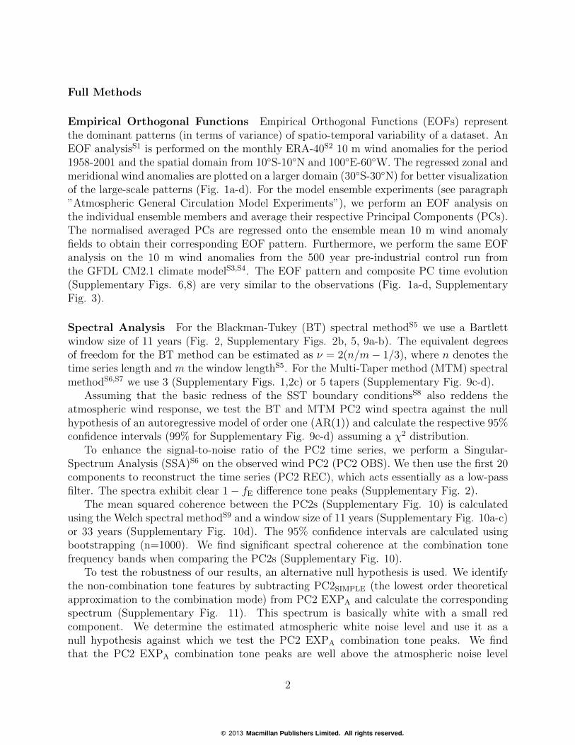
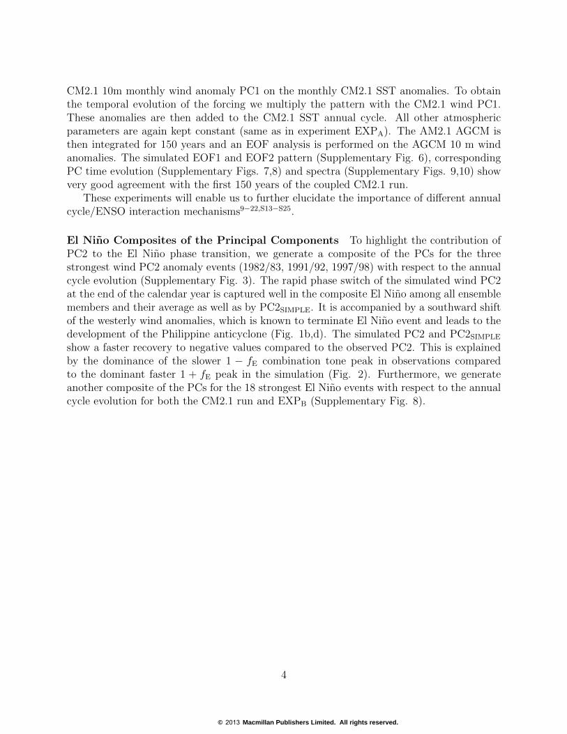
Full Methods

Empirical Orthogonal Functions Empirical Orthogonal Functions (EOFs) representthe dominant patterns (in terms of variance) of spatio-temporal variability of a dataset. AnEOF analysisS1 is performed on the monthly ERA-40S2 10 m wind anomalies for the period1958-2001 and the spatial domain from 10◦S-10◦N and 100◦E-60◦W. The regressed zonal andmeridional wind anomalies are plotted on a larger domain (30◦S-30◦N) for better visualizationof the large-scale patterns (Fig. 1a-d). For the model ensemble experiments (see paragraph”Atmospheric General Circulation Model Experiments”), we perform an EOF analysis onthe individual ensemble members and average their respective Principal Components (PCs).The normalised averaged PCs are regressed onto the ensemble mean 10 m wind anomalyfields to obtain their corresponding EOF pattern. Furthermore, we perform the same EOFanalysis on the 10 m wind anomalies from the 500 year pre-industrial control run fromthe GFDL CM2.1 climate modelS3,S4. The EOF pattern and composite PC time evolution(Supplementary Figs. 6,8) are very similar to the observations (Fig. 1a-d, SupplementaryFig. 3).

Spectral Analysis For the Blackman-Tukey (BT) spectral methodS5 we use a Bartlettwindow size of 11 years (Fig. 2, Supplementary Figs. 2b, 5, 9a-b). The equivalent degreesof freedom for the BT method can be estimated as ν = 2(n/m− 1/3), where n denotes thetime series length and m the window lengthS5. For the Multi-Taper method (MTM) spectralmethodS6,S7 we use 3 (Supplementary Figs. 1,2c) or 5 tapers (Supplementary Fig. 9c-d).

Assuming that the basic redness of the SST boundary conditionsS8 also reddens theatmospheric wind response, we test the BT and MTM PC2 wind spectra against the nullhypothesis of an autoregressive model of order one (AR(1)) and calculate the respective 95%confidence intervals (99% for Supplementary Fig. 9c-d) assuming a χ2 distribution.

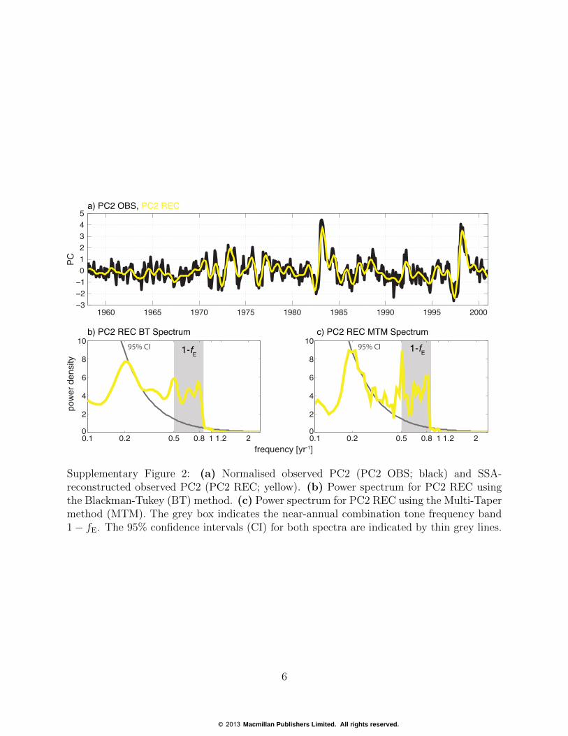
To enhance the signal-to-noise ratio of the PC2 time series, we perform a Singular-Spectrum Analysis (SSA)S6 on the observed wind PC2 (PC2 OBS). We then use the first 20components to reconstruct the time series (PC2 REC), which acts essentially as a low-passfilter. The spectra exhibit clear 1− fE difference tone peaks (Supplementary Fig. 2).

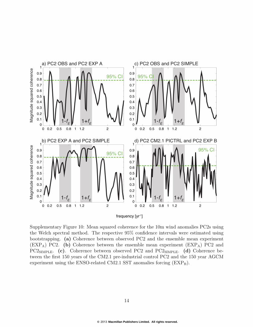
The mean squared coherence between the PC2s (Supplementary Fig. 10) is calculatedusing the Welch spectral methodS9 and a window size of 11 years (Supplementary Fig. 10a-c)or 33 years (Supplementary Fig. 10d). The 95% confidence intervals are calculated usingbootstrapping (n=1000). We find significant spectral coherence at the combination tonefrequency bands when comparing the PC2s (Supplementary Fig. 10).

To test the robustness of our results, an alternative null hypothesis is used. We identifythe non-combination tone features by subtracting PC2SIMPLE (the lowest order theoreticalapproximation to the combination mode) from PC2 EXPA and calculate the correspondingspectrum (Supplementary Fig. 11). This spectrum is basically white with a small redcomponent. We determine the estimated atmospheric white noise level and use it as anull hypothesis against which we test the PC2 EXPA combination tone peaks. We findthat the PC2 EXPA combination tone peaks are well above the atmospheric noise level

2


(Supplementary Fig. 11). Hence, we are able to reject both the red noise (Fig. 2b) andwhite noise (Supplementary Fig. 11) null hypotheses.

Atmospheric General Circulation Model Experiments To test the combinationmode hypothesis we conduct a sensitivity experiment EXPA with the Atmospheric Gen-eral Circulation Model (AGCM) AM2.1S10. The model, used here in a horizontal resolutionof 2◦ latitude and 2.5◦ longitude, simulates atmospheric dynamics and thermodynamics re-alistically when forced with observed SSTS10. The main objective of the experiment is toquantify the effect of ENSO-related SST anomalies in combination with the SST climatologyon the atmospheric circulation. The ENSO single spatial forcing pattern for AM2.1 is de-rived by regressing the normalised ERA-40S2 10 m wind anomaly PC1 on the monthly SSTanomalies (1958-2001) obtained from the Hadley centre sea ice and Sea Surface Tempera-ture (HadISST1) data setS11. The resulting SST pattern is then multiplied by the normalisedERA-40 wind PC1 to obtain the full spatio-temporal evolution of the temperature field lin-early related to the interannual ENSO mode. These SST anomalies are then added on theobserved climatological mean annual cycle of SST taken from the Reynolds Optimum In-terpolation (OI) SST datasetS12. To enhance the signal-to-noise-ratio of our analysis, a 10member ensemble (identical forcing but perturbed atmospheric initial conditions) of AM2.1hindcast experiments is conducted using the described SST boundary conditions from 1958to 2001. As we are only interested in the interaction of interannual SST anomaly variationswith the annual cycle, all other atmospheric parameters are kept at constant 1982 values(e.g. greenhouse gas concentrations and aerosols). Both EOF1 and EOF2 pattern (Fig.1a-d) and the corresponding PC time evolution (Fig. 1e-f) are captured well by the modelsimulation compared to observations. The main EOF2 pattern difference between the modelexperiment and observations is that the simulated Philippine anticyclone is slightly shiftedwestward and features a reduced amplitude.

Furthermore, we conduct an additional single member sensitivity experiment over thesame period with the same ENSO SST anomaly forcing described above but without aseasonal cycle (PERP). The climatological SSTs and radiative forcing are both kept constantat perpetual autumn equinox conditions, however the ENSO SST anomalies are varying intime exactly as in the sensitivity experiments above. PC2 shows no characteristic phaseshift during boreal winter (Supplementary Fig. 3) and no correlation with the observed PC2(r=0.05), thus demonstrating that the mean annual cycle of SST is a key element for theatmospheric combination mode response. As expected, the corresponding EOF2 does notexhibit the zonal wind anomalies characteristic of the southward wind shift (SupplementaryFig. 4), although it captures parts of the Philippine anticyclone structure (The anticyclonehowever is confined to the far western Pacific and the zonal wind pattern is quasi-symmetricthroughout most of the domain).

To further verify the combination mode hypothesis we conduct another experiment(EXPB) using ENSO-related SST anomalies and the seasonal cycle from the GFDL CM2.1500 year pre-industrial control runS3,S4, which simulates ENSO dynamics reasonably wellS4.We calculate the CM2.1 single spatial SST anomaly pattern by regressing the normalised

3


CM2.1 10m monthly wind anomaly PC1 on the monthly CM2.1 SST anomalies. To obtainthe temporal evolution of the forcing we multiply the pattern with the CM2.1 wind PC1.These anomalies are then added to the CM2.1 SST annual cycle. All other atmosphericparameters are again kept constant (same as in experiment EXPA). The AM2.1 AGCM isthen integrated for 150 years and an EOF analysis is performed on the AGCM 10 m windanomalies. The simulated EOF1 and EOF2 pattern (Supplementary Fig. 6), correspondingPC time evolution (Supplementary Figs. 7,8) and spectra (Supplementary Figs. 9,10) showvery good agreement with the first 150 years of the coupled CM2.1 run.

These experiments will enable us to further elucidate the importance of different annualcycle/ENSO interaction mechanisms9−22,S13−S25.

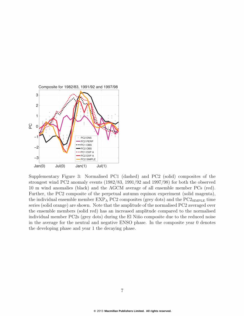
El Nino Composites of the Principal Components To highlight the contribution ofPC2 to the El Nino phase transition, we generate a composite of the PCs for the threestrongest wind PC2 anomaly events (1982/83, 1991/92, 1997/98) with respect to the annualcycle evolution (Supplementary Fig. 3). The rapid phase switch of the simulated wind PC2at the end of the calendar year is captured well in the composite El Nino among all ensemblemembers and their average as well as by PC2SIMPLE. It is accompanied by a southward shiftof the westerly wind anomalies, which is known to terminate El Nino event and leads to thedevelopment of the Philippine anticyclone (Fig. 1b,d). The simulated PC2 and PC2SIMPLE

show a faster recovery to negative values compared to the observed PC2. This is explainedby the dominance of the slower 1 − fE combination tone peak in observations comparedto the dominant faster 1 + fE peak in the simulation (Fig. 2). Furthermore, we generateanother composite of the PCs for the 18 strongest El Nino events with respect to the annualcycle evolution for both the CM2.1 run and EXPB (Supplementary Fig. 8).

4


0.1 0.2 0.5 0.8 1 1.2 202468

10

powe

r den

sity

0.1 0.2 0.5 0.8 1 1.2 202468

10

powe

r den

sity

0.1 0.2 0.5 0.8 1 1.2 202468

10

frequency [yr!1]

powe

r den

sity

PC2 OBS

a) Observations

b) AGCM Reconstruction EXP A

c) PC2 SIMPLE

PC2 95% CI

PC2 AR(1)PC2 EXP A

1-fE 1+fE

1-fE 1+fE

1-fE 1+fE

PC2 95% CI

PC2 AR(1)

Supplementary Figure 1: Power spectra for PC2 using the Multi-Taper method (MTM).Frequency is abbreviated by f . To illustrate the PC2 combination tone frequencies, PC1was shifted to 1 − f (dashed blue) and 1 + f (dashed green) and scaled by a factor 1/3.Grey boxes indicate the near-annual combination tone frequency bands 1 − fE and 1 + fE.The AR(1) null hypothesis for the PC2s in (a)-(b) is displayed by a thick grey line andthe 95% confidence interval (CI) indicated by a thin grey line. (a) Observed PC2 andfrequency-shifted PC1s. (b) Averaged experiment EXPA PC2 and frequency-shifted PC1s.(c) PC2SIMPLE and frequency-shifted PC1s.

5


0.1 0.2 0.5 0.8 1 1.2 20

2

4

6

8

10

pow

er d

ensi

ty

0.1 0.2 0.5 0.8 1 1.2 20

2

4

6

8

10

1960 1965 1970 1975 1980 1985 1990 1995 2000−3−2−1012345

1-fE1-fE

IC %59IC %59

frequency [yr-1]

a) PC2 OBS, PC2 REC

PC

murtcepS MTM CER 2CP )cmurtcepS TB CER 2CP )b

Supplementary Figure 2: (a) Normalised observed PC2 (PC2 OBS; black) and SSA-reconstructed observed PC2 (PC2 REC; yellow). (b) Power spectrum for PC2 REC usingthe Blackman-Tukey (BT) method. (c) Power spectrum for PC2 REC using the Multi-Tapermethod (MTM). The grey box indicates the near-annual combination tone frequency band1− fE. The 95% confidence intervals (CI) for both spectra are indicated by thin grey lines.

6


Jan(0) Jul(0) Jan(1) Jul(1)

−3

−2

−1

0

1

2

3

PC2 ENSPC2 PERPPC1 OBSPC2 OBSPC1 EXP APC2 EXP APC2 SIMPLE

Composite for 1982/83, 1991/92 and 1997/98

PC

Supplementary Figure 3: Normalised PC1 (dashed) and PC2 (solid) composites of thestrongest wind PC2 anomaly events (1982/83, 1991/92 and 1997/98) for both the observed10 m wind anomalies (black) and the AGCM average of all ensemble member PCs (red).Further, the PC2 composite of the perpetual autumn equinox experiment (solid magenta),the individual ensemble member EXPA PC2 composites (grey dots) and the PC2SIMPLE timeseries (solid orange) are shown. Note that the amplitude of the normalised PC2 averaged overthe ensemble members (solid red) has an increased amplitude compared to the normalisedindividual member PC2s (grey dots) during the El Nino composite due to the reduced noisein the average for the neutral and negative ENSO phase. In the composite year 0 denotesthe developing phase and year 1 the decaying phase.

7


[m s-1]

1200E 1600E 1200W 800W1600W

00

100N

100S

200N300N

200S300S

0.75

0

1.6

-1.6

0.8

-0.8

Supplementary Figure 4: EOF2 pattern of the 10 m wind anomalies from the perpetualautumn equinox experiment (12% explained variance). The unit for the zonal wind speed(shading) and 10 m wind vectors is [m s−1].

8


0.1 0.2 0.5 0.8 1 1.2 20

2

4

6

8

10

12

14

frequency [yr -1]

pow

er d

ensi

ty

PC1 PERP

PC2 PERP

PC2 AR(1)

PC2 95% CI

1-fE 1+fE

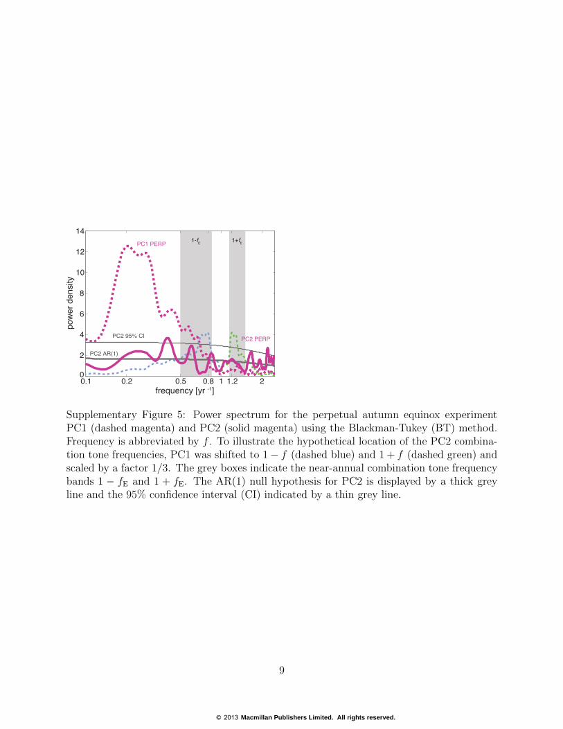
Supplementary Figure 5: Power spectrum for the perpetual autumn equinox experimentPC1 (dashed magenta) and PC2 (solid magenta) using the Blackman-Tukey (BT) method.Frequency is abbreviated by f . To illustrate the hypothetical location of the PC2 combina-tion tone frequencies, PC1 was shifted to 1− f (dashed blue) and 1 + f (dashed green) andscaled by a factor 1/3. The grey boxes indicate the near-annual combination tone frequencybands 1 − fE and 1 + fE. The AR(1) null hypothesis for PC2 is displayed by a thick greyline and the 95% confidence interval (CI) indicated by a thin grey line.

9


00

100N

100S

200N

300N

200S

300S

00

100N

100S

200N

300N

200S

300S

00

100N

100S

200N

300N

200S

300S

00

100N

100S

200N

300N

200S

300S

1200E 1600E 1600W 1200W 800W

1200E 1600E 1600W 1200W 800W

1200E 1600E 1600W 1200W 800W

1200E 1600E 1600W 1200W 800W

1.00

3.00

1.00

3.00 [m s-1]

0

3.50

-3.50

1.75

-1.75

0

2.00

-2.00

1.00

-1.00

a) EOF1 CM2.1 PICTRL (28% variance)

b) EOF2 CM2.1 PICTRL (15% variance)

c) EOF1 AM2.1 EXP B (55% variance)

d) EOF2 AM2.1 EXP B (10% variance)

Supplementary Figure 6: (a)-(d) Dominant pattern of wind variability (zonal wind as shad-ing) in the tropical Pacific obtained by an EOF decomposition of 10 m wind anomalies forthe GFDL CM2.1 500 year pre-industrial control run and a 150 year forced AM2.1 AGCMexperiment (EXPB).

10


PCPC

PC

a) PC1 CM2.1 (black), PC1 EXP B (red)

5 10 15 454035302520 50

55 60 65 959085807570 100

105 110 115 145140135130125120 150

-4-2024

-4-2024

-4-2024

b) PC2 CM2.1 (black), PC2 EXP B (red)

PCPC

PC

-4-2024

-4-2024

-4-2024

time [yr]

5 10 15 454035302520 50

55 60 65 959085807570 100

105 110 115 145140135130125120 150

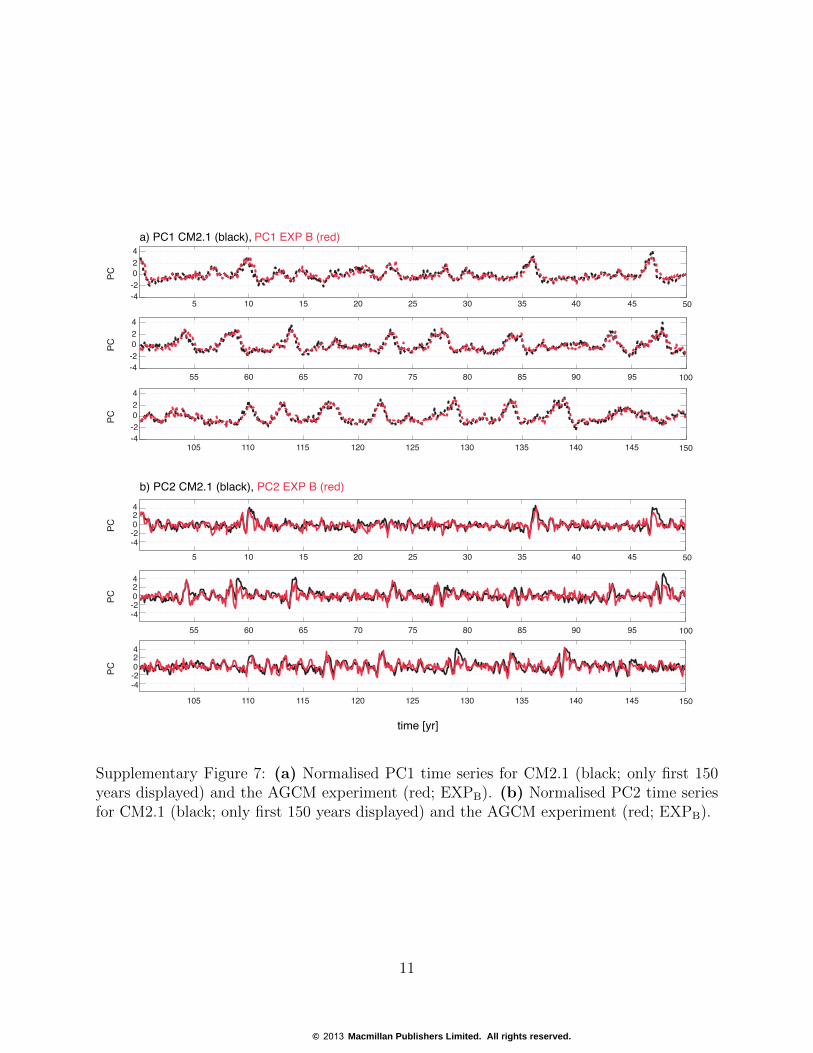
Supplementary Figure 7: (a) Normalised PC1 time series for CM2.1 (black; only first 150years displayed) and the AGCM experiment (red; EXPB). (b) Normalised PC2 time seriesfor CM2.1 (black; only first 150 years displayed) and the AGCM experiment (red; EXPB).

11


Jan(0) Jul(0) Jan(1) Jul(1)−3

−2

−1

0

1

2

3

PC1 CM2.1PC2 CM2.1PC1 EXP BPC2 EXP B

Composite for 18 strongest CM2.1 events

PC

Supplementary Figure 8: Normalised PC1 (dashed) and PC2 (solid) composites of the 18strongest El Nino events in the first 150 years of both the CM2.1 pre-industrial control (black)and the 150 year AM2.1 experiment (red) using the ENSO-related CM2.1 SST anomaliesforcing (EXPB). Year 0 denotes the developing phase and year 1 the decaying phase.

12


0.1 0.2 0.5 0.8 1 1.2 2

pow

er d

ensi

ty

0

2

4

6

8

10

pow

er d

ensi

ty

0

5

10

15a) BT Spectrum CM2.1 500 year PICTRL

b) BT Spectrum 150 year AM2.1 EXP B

0

2

4

6

8

10

0.1 0.2 0.5 0.8 1 1.2 2

0.1 0.2 0.5 0.8 1 1.2 2

0.1 0.2 0.5 0.8 1 1.2 20

5

10

15

frequency [yr −1 ]

c) MTM Spectrum CM2.1 500 year PICTRL

d) MTM Spectrum 150 year AM2.1 EXP B

PC2 95% CI

PC2 CM2.1

PC1 CM2.1 (1-f)

PC1 CM2.1 (1+f)

PC2 95% CI

PC2 99% CI

PC2 99% CI

PC1 EXP B (1-f) PC1 EXP B (1+f)

PC1 EXP B (1+f)

PC1 EXP B (1-f)

PC1 CM2.1 (1+f)

PC1 CM2.1 (1-f)

PC2 CM2.1

PC2 EXP BPC2 EXP B

1-fE 1+fE

1-fE 1+fE 1-fE 1+fE

1-fE 1+fE

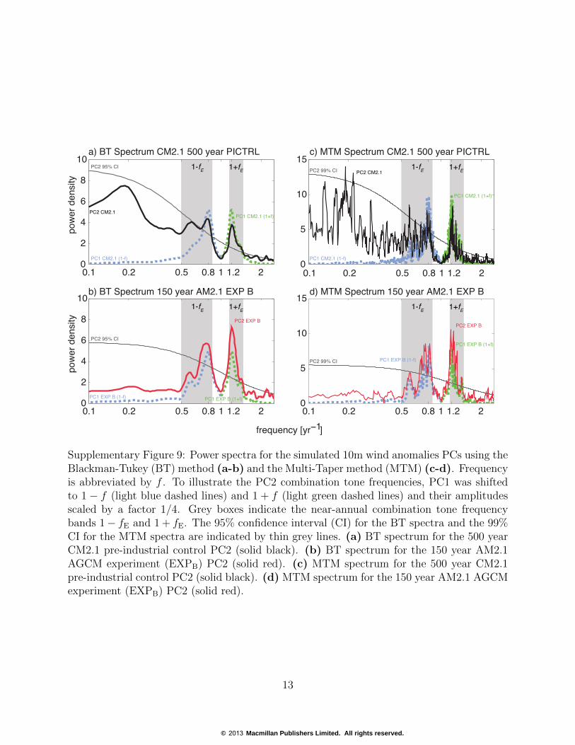
Supplementary Figure 9: Power spectra for the simulated 10m wind anomalies PCs using theBlackman-Tukey (BT) method (a-b) and the Multi-Taper method (MTM) (c-d). Frequencyis abbreviated by f . To illustrate the PC2 combination tone frequencies, PC1 was shiftedto 1− f (light blue dashed lines) and 1 + f (light green dashed lines) and their amplitudesscaled by a factor 1/4. Grey boxes indicate the near-annual combination tone frequencybands 1− fE and 1 + fE. The 95% confidence interval (CI) for the BT spectra and the 99%CI for the MTM spectra are indicated by thin grey lines. (a) BT spectrum for the 500 yearCM2.1 pre-industrial control PC2 (solid black). (b) BT spectrum for the 150 year AM2.1AGCM experiment (EXPB) PC2 (solid red). (c) MTM spectrum for the 500 year CM2.1pre-industrial control PC2 (solid black). (d) MTM spectrum for the 150 year AM2.1 AGCMexperiment (EXPB) PC2 (solid red).

13


Mag

nitu

de s

quar

ed c

oher

ence

0.20.1

0.60.50.40.3

10.90.80.7

0 0 0.2 0.5 0.8 1.21 2

a) PC2 OBS and PC2 EXP A

0.20.1

0.60.50.40.3

10.90.80.7

0 0 0.2 0.5 0.8 1.21 2

0.20.1

0.60.50.40.3

10.90.80.7

0 0 0.2 0.5 0.8 1.21 2

0.20.1

0.60.50.40.3

10.90.80.7

0 0 0.2 0.5 0.8 1.21 2

b) PC2 EXP A and PC2 SIMPLE

c) PC2 OBS and PC2 SIMPLE

d) PC2 CM2.1 PICTRL and PC2 EXP B

95% CI

95% CI

95% CI

95% CI

1-fE 1+fE

1-fE 1+fE

1-fE 1+fE

1-fE 1+fEMag

nitu

de s

quar

ed c

oher

ence

frequency [yr-1]

Supplementary Figure 10: Mean squared coherence for the 10m wind anomalies PC2s usingthe Welch spectral method. The respective 95% confidence intervals were estimated usingbootstrapping. (a) Coherence between observed PC2 and the ensemble mean experiment(EXPA) PC2. (b) Coherence between the ensemble mean experiment (EXPA) PC2 andPC2SIMPLE. (c). Coherence between observed PC2 and PC2SIMPLE. (d) Coherence be-tween the first 150 years of the CM2.1 pre-industrial control PC2 and the 150 year AGCMexperiment using the ENSO-related CM2.1 SST anomalies forcing (EXPB).

14


0.1 0.2 0.5 0.8 1 1.2 20

1

2

3

4

5

6

powe

r den

sity

frequency [yr-1]

White noise level forPC2 EXP A - PC2 SIMPLE

99% CI

PC2 EXP A - PC2 SIMPLEPC2 EXP A

Supplementary Figure 11: Blackman-Tukey spectrum for PC2 EXPA (red line) and PC2EXPA − PC2SIMPLE (blue line) with the atmospheric white noise level corresponding to thelatter (solid grey line) and the associated 99% confidence interval (dashed grey line).

15


Supplementary References

S1. Lorenz, E. N. Empirical Orthogonal Functions and Statistical Weather Prediction (MIT,1956)

S2. Uppala, S. M. et al. The ERA-40 re-analysis. Q. J. R. Meteorol. Soc. 131, 2961-3012(2005). Doi:10.1256/qj.04.176

S3. Delworth, T. L. et al. GFDL’s CM2 global coupled climate models - Part 1: Formula-tion and simulation characteristics. J. Climate 19, 643-674 (2006)

S4. Wittenberg, A. et al. GFDL’s CM2 global coupled climate models - Part 3: TropicalPacific climate and ENSO. J. Climate 19, 698-722 (2006)

S5. Blackman, R. B. & Tukey, J. W. The Measurement of Power Spectra (Dover Publica-tions, 1958)

S6. Ghil, M. et al. Advanced spectral methods for climatic time series. Rev. Geophys. 40,3.1-3.41 (2002)

S7. Thomson, D. J. Spectrum estimation and harmonic analysis. Proceedings of the IEEE70, 1055-1096 (1982)

S8. Hasselmann, K. Stochastic climate models Part I. Theory. Tellus 28, 473-485 (1976)

S9. Welch, P. D. The Use of Fast Fourier Transform for the Estimation of Power Spectra: AMethod Based on Time Averaging Over Short, Modified Periodograms. IEEE Trans.Audio Electroacoust. AU-15, 70-73 (1967)

S10. The GFDL Global Atmospheric Model Development Team. The New GFDL GlobalAtmosphere and Land Model AM2-LM2: Evaluation with Prescribed SST Simulations.J. Climate 17, 4641-4673 (2004). Doi:10.1175/JCLI3223.1

S11. Rayner, N. A. et al. Global analyses of sea surface temperature, sea ice, and nightmarine air temperature since the late nineteenth century. J. Geophys. Res. 108(2003). Doi:10.1029/2002JD002670

S12. Reynolds, R. W. & Smith, T. M. Improved global sea surface temperature analysesusing optimum interpolation. J. Climate 7, 929-948 (1994)

S13. Wang, X. L. The Coupling of the Annual Cycle and ENSO Over the Tropical Pacific.J. Atmos. Sci. 51, 1115-1136 (1994)

S14. Tziperman, E. et al. Irregularity and Locking to the Seasonal Cycle in an ENSOPrediction Model as Explained by the Quasi-Periodicity Route to Chaos. J. Atmos.Sci. 52, 293-306 (1995)

16


S15. Tziperman, E. et al. Mechanisms of Seasonal - ENSO interaction. J. Atmos. Sci. 54,61-71 (1997)

S16. Tziperman, E. et al. Locking of El Nino’s Peak Time to the End of the Calendar Yearin the Delayed Oscillator Picture of ENSO. J. Climate 11, 2191-2199 (1998)

S17. Neelin, J. D. et al. Variations in ENSO Phase Locking. J. Climate 13, 2570-2590(2000)

S18. Galanti E. & Tziperman, E. ENSO’s Phase Locking to the Seasonal Cycle in the Fast-SST, Fast-Wave, and Mixed-Mode Regimes. J. Atmos. Sci. 57, 2936-2950 (2000)

S19. Galanti E. et al. The Equatorial Thermocline Outcropping - A Seasonal Control on theTropical Pacific Ocean - Atmosphere Instability Strength. J. Climate 15, 2721-2739(2002)

S20. An, S.-I. & Wang, B. Mechanisms of Locking of the El Nino and La Nina MaturePhases to Boreal Winter. J. Climate 14, 2164-2176 (2001)

S21. Yan, B. L. & Wu, R. G. Relative roles of different components of the basic state in thephase locking of El Nino mature phases. J. Climate 20, 4267-4277 (2007)

S22. Lengaigne, M. and Vecchi, G. A. Contrasting the termination of moderate and ex-treme El Nino events in Coupled General Circulation Models. Clim. Dyn. (2009)Doi:10.1007/s00382-009-0562-3

S23. Xiao, H. & Mechoso, C. R. Seasonal Cycle-El Nino Relationship: Validation of Hy-potheses. J. Atmos. Sci. 66, 1633-1653 (2009)

S24. Stein, K. et al. Seasonal Synchronization of ENSO Events in a Linear StochasticModel. J. Climate 23, 5629-5643 (2010). Doi:10.1175/2010JCLI3292.1

S25. Ham, Y.-G. et al. What controls phase-locking of ENSO to boreal winter in coupledGCMs? Clim. Dyn. (2012). Doi:10.1007/s00382-012-1420-2

17


A combination mode of the annual cycle and the El Nino ... · Laboratory for Climate Studies, ......

Documents

Transcript of A combination mode of the annual cycle and the El Nino ... · Laboratory for Climate Studies, ......