A Coder's Guide to Elliptic Curve Cryptographyliptic Curve cryptography, may serve as a guide to...
54
Colby College Honors Thesis A Coder’s Guide to Elliptic Curve Cryptography Author: Stephen Morse Supervisor: Fernando Gouvˆ ea A thesis submitted in fulfilment of the requirements for graduating with Honors in Mathematics at Colby College May 2014
Transcript of A Coder's Guide to Elliptic Curve Cryptographyliptic Curve cryptography, may serve as a guide to...

Colby College
Honors Thesis
A Coder’s Guide toElliptic Curve Cryptography
Author:
Stephen Morse
Supervisor:
Fernando Gouvea
A thesis submitted in fulfilment of the requirements
for graduating with Honors in Mathematics at
Colby College
May 2014

COLBY COLLEGE
Abstract
Fernando Gouvea
Colby College - Department of Mathematics and Statistics
Bachelors of Arts
A Coder’s Guide to
Elliptic Curve Cryptography
by Stephen Morse
Many software applications and websites today require a basic understanding of cryptographic
protocols. This work, which is aimed at software engineers and mathematicians interested in El-
liptic Curve cryptography, may serve as a guide to understanding the mathematics and abstract
protocols in Elliptic Curve cryptography. This document is broken up into four sections. The
first describes fundamental concepts in cryptography and gives necessary background informa-
tion. The second covers the mathematics of Elliptic Curves and their complex group structure.
The third describes ECC and implementation details for the ElGamal system. The last section
introduces Diffie-Hellman key exchange and shows how to implement it using Java.

Acknowledgements
To professor Fernando Gouvea, thank you for overseeing my project. Your articulate feedback
and patient guidance was and is extremely appreciated. I have learned so much from you and
I am thankful for the time you committed to helping me with this project.
To professor Justin Sukiennik, I am grateful for your feedback on my thesis and for your help
with LATEX.
To Stephen Jenkins, Byoungwook Jang, and Matt Burton, it has been a great 4 years. I thank
you for keeping my spirits up and my mind sharp.
To Nicole Hewes, your baked goods and heartfelt encouragements were priceless. You kept me
going even when I wanted to quit.
To my family, thank you all for supporting me by coming to my presentation. You convincingly
feigned interest for quite some time and I appreciate it!
ii

Contents
Abstract i
Acknowledgements ii
Contents iii
List of Figures v
List of Tables vi
Preface vii
1 What is Public Key Cryptography? 1
1.1 A Historical Introduction . . . . . . . . . . . . . . . . . . . . . . . . . . . . . . . 1
1.2 A Short Note to the Reader . . . . . . . . . . . . . . . . . . . . . . . . . . . . . 3
1.3 A Mathematical Introduction . . . . . . . . . . . . . . . . . . . . . . . . . . . . . 3
1.4 Example - RSA . . . . . . . . . . . . . . . . . . . . . . . . . . . . . . . . . . . . . 6
1.5 Summary . . . . . . . . . . . . . . . . . . . . . . . . . . . . . . . . . . . . . . . . 8
2 What are Elliptic Curves? 10
2.1 Introduction to Elliptic Curves . . . . . . . . . . . . . . . . . . . . . . . . . . . . 10
2.2 The Group Law on points of an Elliptic Curve . . . . . . . . . . . . . . . . . . . 12
2.3 Derivations and Algorithms for Addition and Negation . . . . . . . . . . . . . . 16
2.4 Elliptic Curves Over Finite Fields . . . . . . . . . . . . . . . . . . . . . . . . . . . 18
2.5 Summary . . . . . . . . . . . . . . . . . . . . . . . . . . . . . . . . . . . . . . . . 21
3 What is Elliptic Curve Public Key Cryptography? 22
3.1 The Elliptic Curve Discrete Logarithm Problem . . . . . . . . . . . . . . . . . . . 22
3.2 Fast Addition Algorithms . . . . . . . . . . . . . . . . . . . . . . . . . . . . . . . 24
3.3 Embedding Messages into E(F2k) . . . . . . . . . . . . . . . . . . . . . . . . . . 25
3.4 Elliptic Curve Cryptography . . . . . . . . . . . . . . . . . . . . . . . . . . . . . 29
3.5 Choosing your Curve . . . . . . . . . . . . . . . . . . . . . . . . . . . . . . . . . 31
3.5.1 Brute Force Attacks . . . . . . . . . . . . . . . . . . . . . . . . . . . . . . 32
3.5.2 Baby-step Giant-Step Algorithm Attacks . . . . . . . . . . . . . . . . . . 33
3.5.3 Pollard’s ρ Algorithm Attacks . . . . . . . . . . . . . . . . . . . . . . . . . 33
3.5.4 Pohlig-Hellman Algorithm Attacks . . . . . . . . . . . . . . . . . . . . . . 34
iii

Contents iv
3.5.5 MOV Algorithm Attacks . . . . . . . . . . . . . . . . . . . . . . . . . . . 34
3.5.6 Anomalous Curve Attacks . . . . . . . . . . . . . . . . . . . . . . . . . . . 35
3.5.7 Weil Descent Attacks . . . . . . . . . . . . . . . . . . . . . . . . . . . . . 35
3.6 Summary . . . . . . . . . . . . . . . . . . . . . . . . . . . . . . . . . . . . . . . . 35
4 Elliptic Curve Cryptography in JavaSE 7 37
4.1 National Security . . . . . . . . . . . . . . . . . . . . . . . . . . . . . . . . . . . . 37
4.2 ECDH Key Exchange . . . . . . . . . . . . . . . . . . . . . . . . . . . . . . . . . 37
4.3 ECDH using Java . . . . . . . . . . . . . . . . . . . . . . . . . . . . . . . . . . . . 39
4.4 Summary . . . . . . . . . . . . . . . . . . . . . . . . . . . . . . . . . . . . . . . . 44

List of Figures
1.1 Alice, Eve, and Bob . . . . . . . . . . . . . . . . . . . . . . . . . . . . . . . . . . 4
2.1 The two types of Elliptic Curves . . . . . . . . . . . . . . . . . . . . . . . . . . . 11
2.2 EllipticCurveAddition . . . . . . . . . . . . . . . . . . . . . . . . . . . . . . . . . 12
2.3 The Point at Infinity . . . . . . . . . . . . . . . . . . . . . . . . . . . . . . . . . . 13
2.4 Associativity of Elliptic Curve Point Addition . . . . . . . . . . . . . . . . . . . . 14
2.5 Doubling a point on an Elliptic Curve . . . . . . . . . . . . . . . . . . . . . . . . 15
2.6 Elliptic Curve Point Negation Pseudocode . . . . . . . . . . . . . . . . . . . . . . 17
2.7 Elliptic Curve Point Addition Pseudocode . . . . . . . . . . . . . . . . . . . . . . 19
3.1 Double-and-Add pseudo code . . . . . . . . . . . . . . . . . . . . . . . . . . . . . 25
v

List of Tables
1.1 Public Key Cryptography Components . . . . . . . . . . . . . . . . . . . . . . . . 6
3.1 Double-and-Add Algorithm . . . . . . . . . . . . . . . . . . . . . . . . . . . . . . 25
vi

Preface
Science is what we understand well enough to explain to a
computer. Art is everything else we do.
- Donald Knuth
As Knuth suggests, real understanding only comes when we can break a complex process down
into its simplest components. Programming languages, the tools for explaining procedures to a
computer, are some of the best tools we have for breaking processes down and systematically
describing each component clearly and concisely.
With this in mind, this work will try to break Elliptic Curve cryptography down into its simplest
components for the reader. By the end, the reader will hopefully understand ECC well enough
that he or she could write an implementation of ECC in a programming language. However, this
work does not cover the syntax for any real programming languages. Instead, we are striving
in this guide for a level of understanding of Elliptic Curve cryptography that is sufficient to be
able to explain the entire process to a computer.
This is guide is mainly aimed at computer scientists with some mathematical background who
are interested in learning more about Elliptic Curve cryptography. It is an introduction to the
world of Elliptic Cryptography and should be supplemented by a more thorough treatment of
the subject. See section 1.2 for a summary of what background material this guide assumes the
reader has already covered.
Happy reading!
vii
Chapter 1
What is Public Key Cryptography?
1.1 A Historical Introduction
World War II was unique for several reasons, among them being the monumental role that
Cryptography took in the communication between military groups, largely due to new crypto-
graphic tools which the technology of the time enabled. Naturally, the opposing military forces
desired fast and accurate communication between their respective allies, while simultaneously
wishing to ensure complete secrecy from their enemies. It is a common theme in the world of
Cryptography, however, that these two features (convenience and security) are in opposition to
each other. When opposing military forces became privy to confidential information the reper-
cussions were severe, so there was a huge need to protect one’s algorithms for sharing secret
information. Great effort was put into doing just that, and thus World War II became not just
a war between physical forces but also between mental and mathematical ones.
One example of an emerging technology that gave groups the power to communicate securely,
for a time at least, was the Enigma machine. It was a small machine that looked somewhat like
a typewriter, and it worked by scrambling the letters of the alphabet according to its current
settings. The trick, however, was that with each keystroke the settings would change, creating
a seemingly random sequence of letters. To decode a message, all one had to do was start the
enigma machine with the exact same settings as the initial encoding settings and then type the
ciphertext into it. Many thought this system to be unbreakable due to the sheer number of
possible settings that the machine could have (well into the trillions) [1]. However, due to the
efforts of Polish mathematicians and many British code-breakers, methods to reliably decode
1

Chapter 1. What is Public Key Cryptography? 2
messages created by the Enigma machine were discovered in 1940. These efforts were not made
public knowledge until the 1970s [2, p. 36].
Do you notice something strange about the Enigma machine’s procedure? It required both the
sender and the receiver to already have a bit of shared information: what settings to start the
Enigma machine at in order encode and decode messages. That is, in order to share secret
information one had to first share secret information! This raises the question: how does one
share the first information securely? This type of cipher, where both the sender and receiver
have a small bit of shared information in order to share larger amounts of secret information, has
become known as a Symmetric Cipher. While typically more secure and efficient, Symmetric
Ciphers are very inconvenient, and in particular is not directly suitable for many web-based
applications where the two parties which need to exchange sensitive information have never met
and so have not had a chance to exchange their own private key.
How can one exchange information securely with someone whom they have never met? The
solution is to create a system by which any two users can share their secret information over an
insecure line of communication. This seems impossible, but, surprisingly, it is not! That is, it is
possible if you assume that anyone listening in on your communication has a realistic amount
of computing power and has not developed any radically new cryptanalysis (code-breaking)
procedures. In most cases, these are reasonable assumptions.
These procedures to share information between users which have never met and over commu-
nication channels that may be monitored fall under the category of Public Key Cryptography.
Such systems are based on mathematical problems that are presumed to be hard for their se-
curity. That is, to crack these systems would require solving a mathematical problem which is
believed to be computationally difficult. In these systems, users will typically each have two
keys: a private key and a public key. The procedure for using these keys is also made public
knowledge so that anyone may send a message to any other individual. This has the unfortunate
side effect that anyone who may be eavesdropping may be assumed to know the exact method
for encoding a secret message using a public key, but fortunately there are algorithms that are
extremely hard to undo, even if one knows how they were performed.
Ciphers which use Public Key Cryptography are called Asymmetric ciphers because the sender
and the receiver do not share the same information. Users are typically aware of all of the other
users’ public keys but each user’s private key is kept secret. While less efficient than Symmetric
ciphers, Asymmetric ciphers have a distinct advantage in that they allow users to share secret

Chapter 1. What is Public Key Cryptography? 3
information even if someone is listening to the entire ‘dialogue’. Typically, these types of ciphers
may be combined: the Asymmetric cipher allows the sharing of a private key and the private
key may then be used with a Symmetric cipher for further communication.
1.2 A Short Note to the Reader
This guide will make an attempt to explain things as carefully as possible, but studying the-
oretical Public Key Cryptography, and Elliptic Curve Cryptography in particular, really does
require some mathematical background. It will be assumed that the reader has at least a basic
understanding of Number Theory and Abstract Algebra. In particular, the reader should be
familiar with modular arithmetic, Fermat’s Little theorem, the Chinese Remainder Theorem,
Groups, and Finite Field theory. For a basic introduction to these topics I recommend looking
at [2]. This great book on Mathematical Cryptography contains short chapters specifically de-
voted to bringing the reader up to speed on some of the background information necessary for
studying Cryptography.
1.3 A Mathematical Introduction
Before we jump right into the mathematics behind Public Key Cryptography, some introduc-
tions are in order. In studying Cryptography, one regularly talks about a few fictional characters
named Alice, Bob, and Eve. As depicted below, the usual story is that Alice and Bob would
like to be able to share confidential messages with each other, but Eve (the eavesdropper) is
listening to every word they say. Having these characters in one’s pocket can help to simplify
the description of crypto-systems.
Now suppose, as we always do, that Alice would like to send Bob a message. Let’s say she
wants to send the message “Hi!”. The first step is for Alice to turn her message into a number
that can then be mathematically manipulated. There are many ways to do this, one being to
use the standard ASCII or Unicode mapping, both of which are built into computers. Another,
would be to simply replace “A” by 10, “B” by 11. . . and so on, so that the message “ABC”
would become the number 101112. This translation from strings to integers and back is not
particularly complicated, so for the remainder of this chapter we will assume that the messages

Chapter 1. What is Public Key Cryptography? 4
Figure 1.1: Alice uses a symmetric cipher to send secret messages to Bob, which Eve is unableto decipher. Source: [3]
that Alice and Bob are trying to send to one another are numerical integers in some defined
range. However, when we get to Elliptic Curve cryptography, we will need to find more clever
ways of embedding our messages (see section 3.3 for more details).
Now we will describe, in an abstract way, the components necessary for Public Key Encryption.
To do this, we needs some definitions.
Definition 1.1. A message is simply information which one person would like to send to
another. Typically these are integers within a certain range. We will let M be the set of all
possible messages for a given cipher.
Definition 1.2. A key is a value, which may either be secret or public knowledge, that is used
in the encryption or decryption of a message. We will let K be the set of all possible keys for a
given cipher.
Definition 1.3. A ciphertext is a value that is created using an encryption algorithm. We
will let C be the set of all possible ciphertexts for a given cipher.
The first step in creating a Public Key cipher is for every one to agree on two functions, an
Encryption function E(kpub,m) : K ×M → C and a Decryption function D(kpriv, c) : K × C →
M. After this, each user picks a private key from K and they make sure that this key is not
shared with anyone else. Using their private key, each user can then calculate which public
key corresponds to their private key and post their that key to a pubic database. After Alice
and Bob have completed this procedure, if Alice would like to send a message m to Bob she
looks up his public Key kBpub, encrypts the message by calculating E(kBpub,m). When she sends
this encrypted message, only Bob, with his secret information kBpriv, will be able to decode her
message.

Chapter 1. What is Public Key Cryptography? 5
Clearly, if our encryption and decryption functions are to be made properly they must satisfy
a certain set of conditions. These conditions are summarized below.
(1) First, we require that the decryption undoes the encryption, as this is necessary for the
entire process to even work at all. That is, it must be the case that for a user’s set of keys
(kpriv, kpub), we have that D(kpriv, E(kpub,m)) = m. Note that this does not mean that the
users may pick any (kpriv, kpub) pair they like, but rather that the E and D functions need to be
functions such that many such pairs exist. Typically, one chooses a private key first, computes
what the public key should be and then publishes the public key. Note that for the system to
be secure at all, knowing kpub should not reveal kpriv.
(2) Second, we need our functions to be easy to compute, as this process will be no good at
all if we cannot share many messages quickly. The determination of how quick one needs it to
be depends one’s own constraints, such as whether the message sender or receiver is using a
computer.
(3) Lastly, we do not want any E functions which reveal information about kpriv or m. In other
words, we require that it be extremely difficult to compute both kpriv and m, even if one knows
the values of kpub and E(kpub,m).
Now, suppose that we have given to us two such functions as described above. First we make
them public for all the world to see. Then anyone who would like to receive messages may
choose a kpriv ∈ K, calculate the associated public key kpub and publish it. Suppose that Alice
and Bob would like to share a message, and their keys are as given in Figure 1.1. If Alice wants
to send her message m to Bob, then all she must do is compute c = E(kBpub,m) and send it to
Bob. Bob, who is the only one who knows kBpriv, will then be able to decode and receive Alice’s
message by computing m = D(kBpriv, c).
The remarkable thing about this process is that after Alice has encrypted her message, not even
she can decode it! Granted, yes, she probably remembers what the message originally was, but
the point is that even she cannot come up with an algorithm to decode her own message. This
is because, by property (3), she cannot is not able to gain any information about kpriv, which is
necessary for the decryption.

Chapter 1. What is Public Key Cryptography? 6
Alice Bob
Private Key kApriv kBpriv
Public Key kApub kBpub
Table 1.1: All members have a their own public key and their own private key.
1.4 Example - RSA
After much talk about these mysterious E and D functions, it is time for an example. The
reader should note that such a system is not easy to create. It was actually postulated that
such a system could exist for quite some time before anyone was actually able to produce an
example. RSA was one of the first examples provided of such a system. The original patent for
this system can be found at [4].
Standard RSA (as created by Rivest, Shamir, and Adleman) is one the simpler examples of a
Public Key system. RSA has also withstood the test of time. That is, no one has been able
to devise an efficient method to break all cases of RSA [5]. Some parameters must be chosen
wisely to thwart known methods of attack, but being careful as to what parameters we choose
is a small inconvenience.
Suppose that someone gives you two prime numbers, 37 and 71, and asks you to compute their
product. You would likely pull the pencil out from behind your ear, scratch away at a piece of
paper for a moment, and then come up with the answer 2, 627. Now suppose that instead of
the numbers 37 and 71, someone gives you the number 2, 627 and asks you to factor it. What
would be your first step? You would likely sit down and try, one by one, each prime less than√2627 ≈ 51.3 until you got to 37, but this would likely take you much longer than multiplying
the two numbers did! This illustrates how much harder factorization is than multiplying, and
this sort of a one way process (a function that easy to compute but difficult to invert) can be
useful for cryptographic purposes.
RSA encryption takes advantage of the fact that even if someone knows the product N = p · q,
where p and q are two large primes, it would be very difficult for him or her to gain any
knowledge of p or q. Thus, if Bob wants to allow others to send him messages, he picks two
large primes p and q, calculates N = p · q, and now N can safely be included in Bob’s public
key. We will need one more bit of information for encryption: a public exponent e chosen in the
range 1 < e < α with the property that gcd(e,α) = 1, where α = (p − 1)(q − 1). Since Bob is
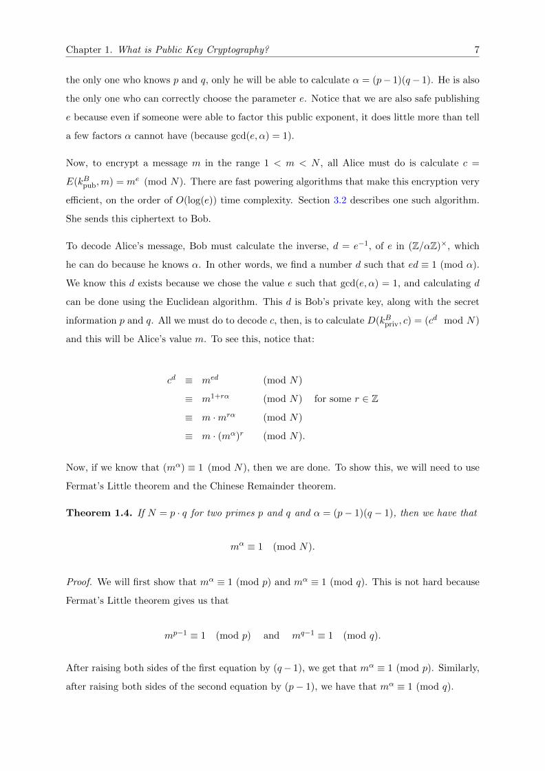
Chapter 1. What is Public Key Cryptography? 7
the only one who knows p and q, only he will be able to calculate α = (p− 1)(q− 1). He is also
the only one who can correctly choose the parameter e. Notice that we are also safe publishing
e because even if someone were able to factor this public exponent, it does little more than tell
a few factors α cannot have (because gcd(e,α) = 1).
Now, to encrypt a message m in the range 1 < m < N , all Alice must do is calculate c =
E(kBpub,m) = me (mod N). There are fast powering algorithms that make this encryption very
efficient, on the order of O(log(e)) time complexity. Section 3.2 describes one such algorithm.
She sends this ciphertext to Bob.
To decode Alice’s message, Bob must calculate the inverse, d = e−1, of e in (Z/αZ)×, which
he can do because he knows α. In other words, we find a number d such that ed ≡ 1 (mod α).
We know this d exists because we chose the value e such that gcd(e,α) = 1, and calculating d
can be done using the Euclidean algorithm. This d is Bob’s private key, along with the secret
information p and q. All we must do to decode c, then, is to calculate D(kBpriv, c) = (cd mod N)
and this will be Alice’s value m. To see this, notice that:
cd ≡ med (mod N)
≡ m1+rα (mod N) for some r ∈ Z
≡ m ·mrα (mod N)
≡ m · (mα)r (mod N).
Now, if we know that (mα) ≡ 1 (mod N), then we are done. To show this, we will need to use
Fermat’s Little theorem and the Chinese Remainder theorem.
Theorem 1.4. If N = p · q for two primes p and q and α = (p− 1)(q − 1), then we have that
mα≡ 1 (mod N).
Proof. We will first show that mα ≡ 1 (mod p) and mα ≡ 1 (mod q). This is not hard because
Fermat’s Little theorem gives us that
mp−1 ≡ 1 (mod p) and mq−1 ≡ 1 (mod q).
After raising both sides of the first equation by (q− 1), we get that mα ≡ 1 (mod p). Similarly,
after raising both sides of the second equation by (p− 1), we have that mα ≡ 1 (mod q).

Chapter 1. What is Public Key Cryptography? 8
Now, we know from the Chinese Remainder Theorem that all solutions to the relations mα ≡
1 (mod p) and mα ≡ 1 (mod q) give values for mα that equivalent mod N . Since mα = 1 is a
solution to these two relations, it must me that mα ≡ 1 (mod N). This completes the proof
that mα ≡ 1 (mod N).
Therefore, the decryption undoes the encryption process, just as we would like it to. This
completes the description of the RSA Public Encryption scheme. To summarize, the encryption
and decryption functions are as below.
E(kBpub,m) = me (mod N)
D(kBpriv, c) = cd (mod N).
As a final note, the security of this system does not only depend on being able to factor N . If
Eve could factor N , she would definitely break the system because then she would easily be able
to compute α and d, which would allow her to decode ciphertexts. But what if someone could
regain the value of m just from knowing c = me (mod N)? Many people have looked for ways
to do this efficiently, but no one has found an efficient algorithm to always solve this problem.
Hence, we say that RSA relies on the difficulty of mathematical problems which are presumed
to be computationally hard because no one has been able to solve them yet. In fact, no attack
on RSA has proved to be easier than factoring N and it can be shown that any algorithm to
break RSA will also factor N . Thus, as long as we have no efficient method for factoring N ,
RSA will remain secure.
1.5 Summary
The Public Key encryption process is a counter-intuitive scheme. It a strange system in which
one cannot even decode one’s own ciphertext, but rather the ciphertexts are furnished in such
a way that only the person they were created for can decode them. It also relies on the
presumption that certain problems are computationally difficult to solve, unless one has some
extra information, for its security. For most encryption schemes we do not actually have a proof
that a breaking the system is hard.

Chapter 1. What is Public Key Cryptography? 9
Public Key encryption is useful because it allows parties that have never met to share small
amounts of confidential information. Many times that small amount of information is a private
key which can be used in a more efficient symmetric cipher.
RSA is an example of an Asymmetric cipher. Although the parameters must be chosen wisely,
RSA seems to be very secure if implemented correctly. Part of the beauty of Public Key en-
cryption schemes like RSA is that even though the value of the encrypted message is completely
determined by the values of the ciphertext and public key, (assuming the parameters are chosen
well) no one will likely have the computing power to be able to find it!

Chapter 2
What are Elliptic Curves?
2.1 Introduction to Elliptic Curves
Elliptic curves, as they are unfortunately named, do not have much to do with Ellipses. Although
Elliptic Curves were originally discovered while studying the properties of Ellipses, they are now
important enough mathematical objects in their own right that a whole field of mathematics is
devoted to them and can be studied without knowledge of how they relate to Ellipses at all.
An Elliptic Curve is the curve given by the set of points which satisfy an equation of the form
y2 + a1xy + a3y = x
3 + a2x2 + a4x+ a6,
where the coefficients must satisfy a complicated polynomial condition to guarantee that the
curve is nonsingular (having no cusps or self-intersections). The above form is known as the
generalized Weierstrass form for Elliptic Curves. The subscripts on the coefficients are chosen
so that the above equation is homogeneous (all terms have the same weight) when x is given
weight 2 and y is given weight 3.
If a1 = 0 then when working over fields with characteristic 2 (which we will mainly be concerned
with), E is what is known as a supersingular curve. This is a property which we will avoid for
reasons to be explained in section 3.5. There are Elliptic curves with a1 = 0, but we are just
not going to work with them as they allow certain attacks that do not work on other types of
curves.
10

Chapter 2. What are Elliptic Curves? 11
The reader should be careful not to confuse singular and supersingular. These two conditions
are less related than their names might suggest. Singularity is a condition on the shape of the
curve which guarantees that it has no cusps or self-intersections. All Elliptic Curves are by
definition non-singular to ensure certain properties of the curves. Supersingular curves are a
special class of Elliptic Curves which we will cover in chapter 3.
For a1 �= 0 (the non-supersingular case over fields of characteristic 2), there is a change of
variables that will take us from the generalized Weierstrass form to a simplified form:
y2 + xy = x
3 + ax2 + b.
In this simplified form, the nonsingularity condition is easier to state: we must be using a curve
with non-zero b. This ensures that certain operations with points of the curve work well. The
change of variables, which assumes that a1 �= 0, is given by:
x → a21x+ a3a1
y → a31y + a−31 (a21a4 + a23).
Although in practice we will use curves written in the simplified form y2+xy = x3+ax2+ b, in
examples I will use equations of various other forms that are easier to work with and to visualize
over R. Elliptic curves come in two main varieties, curves that have two parts and curves that
only have one part. See the figures below for examples of the two varieties.
Figure 2.1: The two types of Elliptic Curves. The left curve is given by y2 = x3 − 2x and theright curve is given by y2 = x3 − x+ 2.

Chapter 2. What are Elliptic Curves? 12
2.2 The Group Law on points of an Elliptic Curve
These curves are special because they come with an operation under which the points on the
curve form a group. The operation is most easily described geometrically. Take two points on
the curve with distinct x-coordinates, call them P and Q. If we extend a line through P and
Q, this line will intersect the curve at a third point, call it R�. We will define the sum P +Q to
be the second point on the curve that has the same x-coordinate as R� has. This point R will
either be directly above or directly below R�. For an illustration of this process, see the figure
below (figure 2.2).
Figure 2.2: Elliptic Curve given by y2 = x3 − 2x with addition of points.
There are still quite a few details to be sorted out, such as how to add a two points with the
same x-coordinate and how we can be sure that there will always be a third point of intersection,
but think about how surprising this should be: under this strange operation, the points of the
curve form a commutative group! That means there is a zero-element, there are inverses, and
that the addition is even associative. This seems to be a bizarre coincidence that there is such
a nice operation on these points, but there is some deep mathematics hiding in the background.
For the interested reader, there is actually an association between the points of an elliptic curve
and the points in the fundamental domain of a lattice in C. In addition, adding modulo the
lattice actually corresponds to adding points on the Elliptic curve. This addition in the lattice
is somewhat more natural, the surprising part is that there is a geometric description of adding
corresponding points on an Elliptic Curve at all. For more on this, see [6].

Chapter 2. What are Elliptic Curves? 13
Now we will sort out some of the subtleties in Elliptic Curve point addition. We first check that
the points on the curve with respect to this operation really do form a commutative group. It
is clear that this operation is commutative, since the operation is not defined in terms of which
point is used first in the addition, but seeing that the points of an Elliptic Curve actually a
group is not quite as easy. Along the way we will further clarify how the addition works, and
at the end of this section we will provide the general algorithm.
(Identity Element) First, there must be an identity element O such that for any point P on
the curve, P +O = P . One way to think about where this element must be is to think of it as
living on the curve, but all the way at at the end of the curve, infinitely far away. For example,
in figure 2.3, the arrows point along the curve, approaching the identity element, sometimes
called the point at infinity.
Figure 2.3: Elliptic Curve together with its point at infinity.
Then, one might think of adding a point P to the point at infinity O as:
limQ→O
(P +Q).
Eventually, Q will be so far above P that the horizontal distance that it has travelled will be
insignificant compared to how large the vertical gap is between the points. Thus, it looks just
as though Q is right above P , and so the third point of intersection will be extremely close to
the point directly opposite from P . Then, according to the geometric definition of the addition
law, we just get back the point P because it is directly opposite the third point of intersection.

Chapter 2. What are Elliptic Curves? 14
One may equivalently think of the point at infinity as being on every vertical line, which makes
it easier to visualize the addition but makes it less clear that the point is actually on the curve.
(Inverse Elements) Verifying the existence of inverses for any point P on the curve is easy
now that we know what our zero element is: −P is just the point with the same x - coordinate
as P , directly above or below it. The line which intersects P and −P will always be vertical,
extending all the way to the point at infinity. Reflecting the point at infinity simply gives back
the same point at infinity (−O = O), showing that P + (−P ) = O.
(Associativity) The last part of the group law to verify is the associativity of the operation.
This can be done one of two ways. The first is to use a brute force approach where one breaks
the addition up into many cases, computes the general formula for P +(Q+R) and (P +Q)+R
for each of the cases, and verifies that they are equal in each case. Verifying this proof would
be an extremely tedious and unenlightening task. The second is to used advanced methods to
relate lattices and Elliptic Curves to prove the associativity, but this is beyond the scope of
this project. We will take this result as known. The reader may look to [6] to see some of the
theory relating Elliptic Curves to lattices. See figure 2.4, to see an example of the associativity
of Elliptic Curve point addition.
Figure 2.4: Associativity of Elliptic Curve Point Addition
The two remaining loose ends are how to add a point to another point with the same x-coordinate
and how we can be sure that there will always be a third point of intersection.
(1) There are two possible cases when adding a point P which has the same x-coordinate as
a point Q. If they have different y-coordinates, then the points are in fact additive inverses of
each other and the third point of intersection on the curve is the point at infinity. In the other
case, P and Q have he same y-coordinate and we are simply looking to find 2P . Similar to how

Chapter 2. What are Elliptic Curves? 15
the addition with the point at infinity was defined, we can define 2P as:
limQ→P
(P +Q).
Eventually P and Q are very close to one another, and in the limit, the line between P and Q
approaches the tangent line of the curve at P . Accounting for multiplicity of intersections, the
tangent line will intersect the curve twice at P and will intersect the curve in one other place,
call it −R (this will be O if P has a vertical tangent line). The addition of the point P to itself,
denoted 2P , is R. See figure 2.5 for a visual.
Figure 2.5: Doubling a point on an Elliptic Curve
(2) It is not extremely difficult to see that the any line that intersects the curve in two places
must intersect it in a third when we include the point at infinity. Suppose we are given the
points P and Q. Let L given by ax+by+c = 0 be the line that intersects the curve at P and Q.
If L is vertical (in which case b = 0) then the third point of intersection is the point at infinity,
O.
Otherwise, we know that b �= 0 and we may write our line in the form y = λx + v. Note that
λ may be obtained as the slope between two distinct points or as the slope of a tangent line of
the curve. In this case, to find the third point of intersection we must find all solutions to the
equation:
(λx+ v)2 + x(λx+ v) = x3 +Ax
2 +B.

Chapter 2. What are Elliptic Curves? 16
Or, equivalently, after some rearranging:
0 = x3 + (A− λ
2− λ)x2 + (−λv − v)x+ (B − v
2).
This is a cubic which we already know two of the roots of, namely the x-coordinates of P and
Q, because we already know two of the points of intersection between the curve and the line.
This means that there must be a third point of intersection because a cubic can only have either
1 or 3 real roots, and since we know it has at least 2, it must be that this cubic actually has 3
real roots.
2.3 Derivations and Algorithms for Addition and Negation
So far we have developed some intuition for Elliptic Curve point operations, but it will be helpful
for automating elliptic curve addition to have explicit formulas for the addition and negation of
points. The derivation and pseudocode for each of these operations is summarized below.
(Negation) Given a point P , we aim to find the point −P such that P + (−P ) = O.
If P = O then −P is also O. Otherwise, P has x and y coordinates Px and Py that satisfy the
given Elliptic Curve equation. The negative of P is the second point on the curve with the same
x-coordinate as P . We can find the two points on the Elliptic Curve that have x-coordinate Px
by plugging in Px for x in our Elliptic Curve Equation:
y2 + Pxy − (P 3
x +AP2x +B) = 0.
We know that the sum of the roots of this equation is −Px and we know that one of the roots
is Py. Thus, Py + (−P )y = −Px, which tells us that:
(−P )y = −Px − Py.
And if we are working in a field K with characteristic 2, meaning that for any k ∈ K 2k = 0,
then the above equation is equivalent to:
(−P )y = Px + Py.

Chapter 2. What are Elliptic Curves? 17
We will use this definition because we will be working with fields of characteristic 2, where there
is no difference between adding or subtracting an element of the field. The pseudocode summary
of this calculation is below. Note that in this pseudocode, we use 0 both as the identity element
of the field we are working with and as the identity element of the group of points on an Elliptic
Curve. The reader should be able to tell from the context which additive identity it is that 0 is
playing the role of in each line of pseudocode.
Figure 2.6: Elliptic Curve Point Negation Pseudocode for Points with Coordinates in a Fieldof Characteristic 2.
(Addition) Given P and Q, which are any two points on an Elliptic Curve together with the
point at infinity, we aim to find a third point R such that P +Q = R.
By our definition of the addition, if either one of our points is the identity element O, then
the addition is just the other point. In addition, if the points have the same x-coordinates and
different y-coordinates then we know the points are negatives of each other. If they have both
the the same x and y-coordinates and the tangent line at the point is vertical, then the addition
also results in O. These are the base cases which we must get out of the way, the real work
comes in when we are either doubling a point with non-vertical tangent line or we are adding
points with different x-coordinates. We derive the addition formulae for these cases below.
We return to the equation that we saw at the end of section 2.2. This equation has three roots,
each of which corresponds to an intersection between a line and the curve. The line, of course,
is the line with slope λ that connects the two points we are adding (or the non-vertical tangent
line of a point that we are doubling), and we are looking to find the x-coordinate of the third
point of intersection. We have:
0 = x3 + (A− λ
2− λ)x2 + (−λv − v)x+ (B − v
2).
We will use a trick similar to the one that we used in calculating the negative of a point. If we
factor this polynomial completely, which we know we can do because it has 3 real roots, then

Chapter 2. What are Elliptic Curves? 18
we get an equation that contains the three x-coordinates that we are interested in:
0 = (x− Px)(x−Qx)(x−Rx).
If we expand this and then equate the x2 term of both of these polynomials, we will see that it
must be the case that:
−Px −Qx −Rx = A− λ2− λ.
Therefore, we can find the x-coordinate of the third point of intersection Rx by calculating:
Rx = λ2 + λ−A− Px −Qx.
The y-coordinate of −R is clearly given by (−R)y = λRx+v, as we know it lies on the y = λx+v
line. All that is left is to negate the point we have found, −R, using the previously defined
formula for point negation and we have found our point R such that P +Q = R.
Just as before, if we are working with a field of characteristic 2, then these formulas may actually
be adjusted slightly. We have:
(−R)x = λ2 + λ+A+ Px +Qx
(−R)y = λRx + v
R = negative(−R).
The negative function used here is taken to mean the Elliptic Curve point negation algorithm,
which was derived at the beginning of this section. Also as before, 0 is used both in comparisons
with points and in comparisons with point coordinates. The reader should be able to tell from
the context if a 0 is referring to the additive identity of the points on the elliptic curve (pairs of
coordinates) or the additive identity of the field in which the coordinates lie.
Note that there are many computational improvements that could be made for the addition
algorithm described in this section.
2.4 Elliptic Curves Over Finite Fields
The algorithms described in section 2.3 were designed for a field of characteristic 2 in anticipation
of needing such a field for computation gains, but our intuition for addition has been gleaned

Chapter 2. What are Elliptic Curves? 19
Figure 2.7: Elliptic Curve Point Addition Pseudocode for Points with Coordinates in a Fieldof Characteristic 2.
from pictures of the geometric construction over the reals R. One of the remarkable aspects of
Elliptic Curves is that the points of the curve still form a commutative group even when we are
working with a finite field [2, p. 286]. That is, all of the operations that we have described over
R actually still make sense in the language of algebraic geometry, and this language is valid over
any field. The only loss in working over a finite field is that we may no longer nicely visualize
the points on a smooth Elliptic Curve in R2. The gain, however, is that with finite fields we do
not need to have the same amount of precision necessary for ECC over R. In addition we may
even choose our finite fields so as to make the addition on those fields much more efficient in
computer automated implementations.
Clearly, to make use of the massive computing power available to us today we seek to find a
field which we may represent with 0s and 1s. The fields that may be expressed this way most

Chapter 2. What are Elliptic Curves? 20
efficiently are the fields F2m for some m ∈ Z. Elements of a field F2m may be represented as
a polynomial of degree m − 1 with m coefficients that are each either 0 or 1. We will use a
as the variable when describing such polynomials. For example, a2 + 1 ∈ F23 . Equivalently,
we may use the placement of the bits to denote the the power of the term, so we may write
a2 + 1 = 101 ∈ F23 . Notice that using this notation it only takes m bits to store an element of
F2m .
Addition in this field is polynomial addition modulo 2, and multiplication is done by regular
polynomial multiplication followed by reduction modulo an irreducible polynomial of degree m.
The operations in used in calculating Elliptic Curve point addition are done using these two
fundamental operations. It does not matter which irreducible polynomial over F2 of degree m we
choose, different choices will result in the same finite field. However, the representation of certain
elements will look very different for different choices of irreducible polynomials. Standards have
been created so that anyone following these standards will be using the same representation of
the field. These standards are known as the Conway polynomials [7]. We will always use the
standard Conway polynomials for creating the field representation. In addition, we will use the
notation E(F) to denote the group of points with coordinates in F over the Elliptic Curve E.
Example 2.1. Suppose we are working with F23∼= F2[a]/(a3+a+1). We now show an example
of addition with two points of E(F23), P = (a+ 1, a+ 1) and Q = (a, a2 + a), where E is given
by y2 + xy = x3 + (a)x2 + (a2 + 1).
Note that the two points above are points on the curve because:
(a+ 1)2 + (a+ 1)(a+ 1) = (a+ 1)3 + (a)(a+ 1)2 + (a2 + 1)
0 = a2 + 1 + (a2 + 1)
0 = 0
and,
(a2 + a)2 + (a)(a2 + a) = (a)3 + (a)(a)2 + (a2 + 1)
a+ (a2 + a+ 1) = (a2 + 1)
a2 + 1 = a2 + 1.
These points have different x-coordinates so we set
λ =Py +Qy
Px +Qx=
(a+ 1) + (a2 + a)
(a+ 1) + (a)= a
2 + 1.

Chapter 2. What are Elliptic Curves? 21
Then, to calculate the third point of intersection, we first calculate the x-coordinate:
(−R)x = λ2 + λ+A+ Px +Qx
= (a2 + 1)2 + (a2 + 1) + (a) + (a+ 1) + (a)
= 1.
And then we the calculate the y-coordinate of (−R) as:
(−R)y = λ · (−R)x + λ · Px + Py
= (a2 + 1) · (1) + (a2 + 1) · (a+ 1) + (a+ 1)
= a.
And finally, we negate −R = (1, a) to conclude that P + Q = (1, a + 1). This could also be
written as (011, 011) + (010, 110) = (001, 011). The last thing we should do is to check is that
this point in fact is a point on the curve:
(a+ 1)2 + (1)(a+ 1) = (1)3 + (a)(1)2 + (a2 + 1),
(a2 + 1) + (a+ 1) = 1 + a+ (a2 + 1),
a2 + a = a2 + a.
2.5 Summary
The points that satisfy the equation of an Elliptic curve form a group, and the addition law for
that group may be described geometrically. Using this geometric definition of addition, we may
define laws and algorithms for negation and addition of points that extend to finite fields, where
there is not a simple geometric definition of addition. In addition, if we choose to work with
coordinates that are in a field of characteristic 2, then we may efficiently store and manipulate
points with computers.

Chapter 3
What is Elliptic Curve Public Key
Cryptography?
3.1 The Elliptic Curve Discrete Logarithm Problem
Public Key cryptography is built upon problems which are assumed, although not proven, to
be very computationally difficult. In RSA, this problem was factoring a large product of two
primes. Many other Pubic Key encryption schemes are built on the witnessed difficulty of
a problem known as the discrete logarithm problem. The Elliptic Curve Discrete Logarithm
Problem (ECDLP) is a special case of the discrete logarithm problem that is acknowledged to
be even more computationally difficult than the standard discrete logarithm problem [2, p. 296].
Definition 3.1. The discrete logarithm over a group G: Given an element b ∈ G and a power
of b given by g ∈ G, find an integer k such that bk = g.
This called the discrete logarithm problem because of the analogous continuous problem where
one might seek to find a number r ∈ R such that gr = h, where g, h ∈ R and g, h > 0. A
solution to this problem would be denoted as the logarithm logg h. The continuous problem is
much easier than the discrete one, however, because the Taylor series for the natural logarithm
gives a simple converging formula for calculating the r. This formula does not extend to finite
fields, and in general the number e such that ge ≡ h (mod p) looks random. Therefore, the
most natural way to try to solve this problem would be to try every possible value for e, which
is typically computationally infeasible.
22

Chapter 3. What is Elliptic Curve Public Key Cryptography? 23
Example 3.1. Let us use the group Z/11Z under multiplication. It is true that g = 2 is a
generator for this field. We seek to find an e such that 2e ≡ 5 (mod 11).
Without any advanced tools in our tool box (such as the Index Calculus or Sieve methods), we
are stuck trying each value for e until we find one that works.
21 ≡ 2 (mod 11) ×
22 ≡ 4 (mod 11) ×
23 ≡ 8 (mod 11) ×
24 ≡ 5 (mod 11) �
Definition 3.2. The Elliptic Curve Discrete Logarithm Problem over E(F2m): Given P , a
point of E(F2m), and another point Q which is a multiple of P , find an integer n such that
nP = Q.
Note that here the group operation is addition, but this is just a notational difference from the
original DLP. Also notice that we only say an integer n (instead of the integer n) because there
will in fact be infinitely many such integers. This was not necessarily the case in the standard
discrete logarithm problem introduced above because we did not necessarily assume that the
group was finite. In the ECDLP, however, the group is a finite group and so we can show that
there will in fact be infinitely many integers that relate P and Q.
To see this, note that the set {nP : n ∈ Z} must be finite because E(F2m) is finite (having at
most (2m)2 elements). Thus, there will be distinct a, b such that aP = bP . Without loss of
generality, let b be the larger value. Then (b−a)P = O, and so for any one n such that nP = Q
(which we are assuming exist), we also have that (n+c(b−a))P = nP+c(b−a)P = Q+cO = Q,
for any c ∈ Z. This shows that there are in fact infinitely many such integers that will solve
any particular Elliptic Curve DLP, and in fact any one of them will allow an eavesdropper to
decrypt a system which was built using a specific multiple of P .
Example 3.2. Suppose we are working over the field F23∼= F2[a]/(a3 + a + 1) and let E be
given by the equation y2 + xy = x3 + (a)x2 + (a2 + 1). Given P = (1, a + 1) and Q = (a, a2),
We seek to find an integer n such point such that nP = Q.

Chapter 3. What is Elliptic Curve Public Key Cryptography? 24
As an example of what a brute force attack on the ECDLP would entail, we try each integer
until we find an n that relates the two points.
1P = (1, a+ 1) ×
P + P = 2P = (a2, a2 + a) ×
P + 2P = 3P = (a2 + a+ 1, a) ×
P + 3P = 4P = (a, a2) �
3.2 Fast Addition Algorithms
Before we can introduce how to make a crypto-system based on the difficulty of the ECDLP we
need to have an efficient method of calculating nP , where n is some large integer. Obviously, if
encryption involved calculating nP by n distinct additions of P , then it would take just as long
as it would to solve the ECDLP by brute force. So, in order to have any chance of making a
public key system based on the DLP, we must have methods to calculate nP very efficiently.
One such method is known as the Double-and-Add algorithm, which is similar to the method
of successive squaring in modular arithmetic. It works by using the base 2 representation of n,
and is more clearly described with an example than with formulae, although I will provide a
pseudo-code algorithm after the following example.
We will continue working with E be given by the equation y2 + xy = x3 + (a)x2 + (a2 + 1),
but we change the field we are working with to be F25∼= F2[a]/(a5 + a2 + 1). It is not hard to
check that (a2 + 1, a4 + a + 1) is a point on this curve. We will calculate 26P using the base
two representation for 26, which is 11010. Now, notice that:
26P = (24 + 23 + 21)P
= 24P + 23P + 21P.
Start with what will eventually be the result R = 26P by setting R = O. Since the base 2
representation of 26 has a 0 in its first digit (the least-significant digit), we do not add P to
R. Now double P to calculate 2P . Since the base 2 representation of 26 does have a 1 in
its second digit, we do add 2P to R. Then we double 2P to find 4P , which we do not add
to R because there is a zero in the next digit. Double again to find 8P and add to R and
then double again to find 16P and add to R. After this procedure is completed, we find that
26P = (a2 + a, a3 + a2 + a). The results at each step of the process can be seen in table 3.1.

Chapter 3. What is Elliptic Curve Public Key Cryptography? 25
R Power of 2 Digit of 26 Doubles of P
O 0 0 P = (a2 + 1, a4 + a+ 1)O 1 1 2P = (a2 + a, a3)
(a2 + a, a3) 2 0 4P = (a4 + a3 + a2 + 1, a2)(a2 + a, a3) 3 1 8P = (a4 + a3 + a+ 1, a3 + a2 + a+ 1)
(a4, 1) 4 1 16P = (a4 + a, a2 + 1)(a2 + a, a3 + a2 + a+ 1) NA NA NA
Table 3.1: An example of the Double-and-Add algorithm, step by step.
Notice that instead of the 26 additions that it would have taken us to calculate 26P naively,
it only took 4 different doublings and 5 additions, for a total of 9 EC point operations, which
is much better than 26. On average, we will need log2 n doublings and 12 log2 n additions. The
difference between the the two methods becomes much more impressive for larger values of n.
For example, to calculate 1869P for an arbitrary point P would take 17 point operations instead
of approximately 1, 900. This method is very efficient but there are still many improvements
that can be made. For more, see [2].
Figure 3.1: Double-and-Add pseudo code.
Remember, this algorithm relies on the fact that Elliptic Curve point addition is associative.
That is, calculating 26 distinct additions of P as P + (P + (P + · · · + P ) · · · ) is the same as
16P + (8P + 2P ).
3.3 Embedding Messages into E(F2k)
The first step in any cryptographic system is usually to turn one’s message into a number that
can then be mathematically manipulated and encrypted. In ECC, however, we use a set of

Chapter 3. What is Elliptic Curve Public Key Cryptography? 26
points of an Elliptic curve for manipulation and encryption. In this section, we will show a
method to relate simple number messages and the points of an Elliptic curve.
What we would like to have is a one-to-one function that turns a number message into a point on
an Elliptic Curve, and can then be easily inverted after the encrypted point has been decrypted.
If we had such a function, the sender would take his or her message, put it through the function
to get the corresponding point for that message, encrypt it and then send the encrypted point.
Then the receiver would decrypt the message using his or her private key to get a point on the
Elliptic Curve, which they then can invert back into the original number message.
In practice, it is hard to create a fail-safe method for creating a correspondence between number
messages and points of an Elliptic curve. The alternative is to create a probabilistic system which
is extremely likely to work. We will present one way of doing this here, but this is just one
of many possible methods. This method is the characteristic 2 version of one of the solutions
proposed in Koblitz’ paper on Elliptic Curve Cryptosystems [8].
Before a more concrete description of the system, I will do an example. The idea is to sacrifice a
few bits in message length in order to be able to replace those bits with other values so that the
resulting message is an x-coordinate of a point that is on the curve. Remember that elements
of F2k can be represented as a sequence of k bits (where each bit is a 0 or a 1). Suppose we are
working over F2277 , where the coordinates of a point on an Elliptic Curve each take 277 bits to
store. But instead of sending 277 bit messages, we are going to only send 256 bit messages (a
nice even 32 bytes). Now, when finding a point on an Elliptic Curve that has an x-coordinate
that matches a message m, we only need m and the x-coordinate to match in 256 of the 277
bits. The remaining 21 bits will be used freely to make an x-coordinate for which there is a
corresponding y-coordinate of a point on our Elliptic Curve. If Alice uses this method to embed,
encrypt, and then send her message, then after Bob decrypts the message using his private key
he will just throw away the last 21 bits of the message, knowing that Alice made them whatever
she needed to be to find a point on the curve.
This sounds like a reasonable solution, but there are a few practical matters to work out. For
example, how can we be sure that this method will work? That is, if we send messages which
each take i bits to store and there are j bits left over in the k bits of our field (so i + j = k),
how can we be sure there is a sequence of j bits such that m concatenated with the j bits forms
the x-coordinate of a point on the curve? If this method will not always work, then how often

Chapter 3. What is Elliptic Curve Public Key Cryptography? 27
with it fail? How many bits do we need to sacrifice in order to make this message embedding
scheme be reliable? We will work out those details now.
To determine the likelihood that this process will succeed, we need to know when it is that a
random x-coordinate in F2k has at least 1 corresponding y coordinate on the curve. To find a
point on the Elliptic curve, we start with a proposed x-coordinate w ∈ F2k , which matches m
for its first i bits. We first start with the remaining j bits of w bits all being zero. We seek to
find a y ∈ F2k such that:
y2 + wy = w
3 + aw2 + b.
Or, equivalently, that:
y2 + (w)y + (w3 + aw
2 + b) = 0.
Multiplying each size by w−2 (assuming we are not trying to send a string of zeroes), we have
that:�y
w
�2+�y
w
�+
�w + a+
b
w2
�= 0.
We now make a change of variables which we can undo later in order to recover the y-coordinate.
The change of variables is y → wY gives:
Y2 + Y +
�w + a+
b
w2
�= 0.
Given that w �= 0, this quadratic must have either 0 or 2 roots. In [9], Pommerening shows a
method for determining if this quadratic has 0 or 2 roots in F2k . It uses the trace of w in F2.
The trace is defined by:
Tr(w) =k�
i=1
w2i−1
= w + w2 + w
4 + · · ·+ w2k−1
.
This is an element of F2. Pommerening shows that a quadratic of the above form has roots if
and only if Tr�w + a+ b
w2
�= 0. I will denote this value
�w + a+ b
w2
�as ΓE(w). This gives
us a relatively easy algorithm to check whether or not we can use the sequence of j bits that
was used to form w to form a point on E: we just check if Tr(ΓE(w)) = 0. If it is not, then we
increment the value in the j bits and test the algorithm again.
A randomly chosen w ∈ F2k will have Tr(ΓE(w)) = 0 about half the time. This is not proven,
but rather is more of an experimentally observed truth. When every possible w that matches
m for the first i bits has Tr(ΓE(w)) = 1 we fail to turn our number message into a point on an

Chapter 3. What is Elliptic Curve Public Key Cryptography? 28
Elliptic curve. The goal is to make this improbable enough that it will not happen for as long
as the curve is in use.
We can estimate the chance that this probabilistic method will fail by using the estimate that
any given w is likely to have Tr(ΓE(w)) = 0 about 12 of the time. In order for a message to fail
the encryption process, it must fail 2j times, meaning that we have a probability of�12
�2jof
failing to encrypt our message. In the example that we used before where k = 277 and i = 256,
the probability of failing to decrypt a message would be astronomically low:
�1
2
�221
≈ 2.201 · 10−631,306
In practice, it would be wasteful to use j = 21 because we could be using some of those bits
to exchange message data. It is usually sufficient to use j such that 5 ≤ j ≤ 8, but individual
specifications on the need for a fail-safe embedding must be used to determine j.
Example 3.3. Suppose we are working with the field F27∼= F2[a]/(a7 + a+ 1) on the curve E
given by y2 + xy = x3 + (a)x2 + (a2 + 1). Also suppose that our messages have length i = 5
bits and so we have j = 2 free bits. We will find the point on the curve that corresponds to the
number message m = 12.
Write m in base two using i = 5 bits: 01100. We try our first sequence of j bits: 00. Then our
proposed x-coordinate is 0110000, or a5 + a4. We first calculate ΓE(w) below:
ΓE(w) = w + a+ bw2
= (a5 + a4 + 1) + (a) + (a2 + 1)(a5 + a4 + 1)−2
= a3 + a2 + 1.
It is not hard to check that this has trace 1. Since ΓE(w) has trace 1, there is no point on the
curve E that has this x-coordinate, so we need not waste our time looking. Next we try 01 as
our sequence of j bits. Our new proposed x-coordinate is 0110001, or w = a5 + a4 + 1. We
calculate
ΓE(w) = w + a+ bw2
= (a5 + a4) + (a) + (a2 + 1)(a5 + a4)−2
= a6 + a5,

Chapter 3. What is Elliptic Curve Public Key Cryptography? 29
which has trace 0. Now we may look for y-coordinates that can be matched with our w using
algorithms to solve the quadratic in a finite field. For algorithms to do this, see [10]. We find
two points that have w = a5 + a4 + 1 as their x-coordinate:
(a5 + a4 + 1, a6 + 1) and (a5 + a
4 + 1, a6 + a5 + a
4).
Either of these points may serve as the message point for use in our ECC system. After dropping
the last j = 2 bits, they both give the message 01100, or 12.
3.4 Elliptic Curve Cryptography
So far, the key point in this chapter has been that calculating nP is relatively easy (for a com-
puter) compared to finding a value of n relating P and Q = nP . The goal of this section is
to describe how we can turn this hard problem (the ECDLP) into a Public Key Cryptography
system. The system presented here is known as the Elliptic ElGamal System, and was inde-
pendently extended from the standard ElGamal system by Neal Koblitz and by Victor Miller
[11].
In the Elliptic ElGamal system, the group which wishes to communicate securely should publicly
choose an Elliptic Curve, a Finite Field representation and a point which has large order (the
next section goes over how to choose some of these parameters to avoid known attacks on ECC).
We will denote the finite field we are using as F2k for some integer k and the starting point
on the curve as P . Each person that would like to receive messages picks a large integer kpriv
and computes Qpub = kpub = kprivP , which is their public key. Remember that making this
information public is only considered safe because the ECDLP is considered difficult.
The encryption process in Elliptic ElGamal consists of creating a pair of cipher texts from
which only the person with the secret integer kpriv will be able to regain the original message,
which is a point on the chosen Elliptic Curve. The first cipher text, c1, is created by taking a
random large value r and the message point M that one would like to send, and then computing
c1 = M + rQpub. In order to be able to recover the message M , the receiver must be able to
subtract rQpub from c1. The problem, however, is that r cannot be sent by itself or and
eavesdropper would be able to decode the message easily. But rQpub is the value the receiver
really needs in order to decode c1, and rQpub = r(kprivP ) = kpriv(rP ). So if we sent the value

Chapter 3. What is Elliptic Curve Public Key Cryptography? 30
c2 = rP (which we are assuming does not reveal r), then the receiver could use their secret
value kpriv to calculate kpriv · c2, subtract this from c1, and they will recover the value M .
In summary, encryption is done by randomly generating r and then calculating:
c1 = M + rQpub
c2 = rP.
After the receiver has the values c1 and c2, he or she may undo the decryption by calculating:
c1 − kpriv · c2 = M + r ·Qpub − kpriv · r · P
= M + (r · kpriv)P − (r · kpriv)P
= M.
Example 3.4. We will do a sample encryption and decryption using the following parameters.
Suppose we are working over the field F27∼= F2[a]/(a7+a+1) and let E be given by the equation
y2+xy = x3+(a)x2+(a2+1). Then E(F27) consists of 116 distinct points, including the point
at infinity. The point
P = (a6 + a5 + a
3 + 1, a6 + a5 + a
3 + a+ 1)
on this curve will be used in our encryption system. Suppose Alice has the message m = 12,
which was shown in the previous section to correspond to the point M = (a5 + a4 + 1, a6 + 1),
that she would like to send to Bob. Bob has the private key npriv = 97, so his public key is
Qpub = 97P = (a6 + a4 + a3 + a+ 1, a4 + a3 + a2 + a).
Alice calculates her two cipher texts, which are custom made for Bob using his public key Qpub.
She picks a random r = 49 and calculates c1 as:
c1 = M + rQpub
= (a5 + a4 + 1, a6 + 1) + 49 · (a6 + a4 + a3 + a+ 1, a4 + a3 + a2 + a)
= (a5 + a4 + 1, a6 + 1) + (a6 + a4 + 1, a5 + a4 + a2)
= (a, a6 + a5 + a4 + a2 + a).

Chapter 3. What is Elliptic Curve Public Key Cryptography? 31
Using r = 49, she also calculates c2 as:
c2 = rP
= 49 · (a6 + a5 + a3 + 1, a6 + a5 + a3 + a+ 1)
= (a4 + a3 + a2 + a+ 1, a4 + a2 + a).
She sends (c1, c2) to Bob over the insecure channel. Bob can then do the following calculations
to regain Alice’s message, M :
M = c1 − kpriv · c2
= (a, a6 + a5 + a4 + a2 + a)− 97 · (a4 + a3 + a2 + a+ 1, a4 + a2 + a)
= (a, a6 + a5 + a4 + a2 + a)− (a6 + a4 + 1, a5 + a4 + a2)
= (a5 + a4 + 1, a6 + 1).
Knowing that M actually only holds 5 bits of useful message information, Bob drops the last
two bits of the x-coordinate to regain the message m = 01100, which is Alice’s original message.
3.5 Choosing your Curve
The previous section described how to use an Elliptic Curve and other parameters in an Elliptic
ElGamal System in order to secretly share points. But choosing the parameters for an ECC
system is a very delicate process and requires care to avoid certain known attacks on systems
with parameters that have certain properties. The parameters also need to be of a certain size
to have a sufficient security level, and different security levels are required depending on the
sensitivity of the information and on the processing power of modern CPUs (i.e. how much time
and money would an attacker need to invest in order to break the system). This section briefly
summarizes a few known attacks, explains how the existence of each attack should regulate the
choice of parameters, and describes the relationship between the size of the parameters chosen
and their security levels.
We need a measure of security of a certain set of parameters. Usually these measurements of
security are:
(1) Security level - The security level is the number of bits in the number of operations
that would be necessary to break the system using the best (publicly) known algorithm for

Chapter 3. What is Elliptic Curve Public Key Cryptography? 32
breaking the system. This is a measure of how hard it would be to break the system using
the best known methods; the more bits necessary the better the security level. Notice that if
more efficient algorithms are developed, the security for a particular system may decrease even
though the system has not changed. In this sense, the security level is a reflection of how hard
an adversary would have to work to break the system if they were using the best publicly known
algorithm.
(2) Key size - For a given system with specified parameters, the Key size is the number of bits
necessary to store a key for the system, usually the private key in Public Key Cryptography.
This also represents the highest possible security level, because any system can be broken by
testing every possible private key (see 3.5.1). Since there are usually faster algorithms than
the brute force approach, however, the Security level will likely be less than the Key size. The
higher the key size, the harder encryption and decryption will be. Essentially, the Key size is
a measure of how hard the users of the system have to work and how much data they have to
store in order to implement the cryptographic system.
Cryptographic systems always have to balance the key size with the security level. If the
parameters are chosen to be too small then the Security level will be too small and too easy for
an attacker to break. If the parameters are chosen to be too large, however, then the Key size
will be too large to be able to use the system efficiently or on a large scale.
An Elliptic Curve E over the finite field F2m has key size m because that is how many bits it
will roughly take to store a private key in ECC. The best known algorithm to solve the ECDLP
in a well-chosen Elliptic Curve finishes in roughly√2m = 2
m2 steps, so the Security Level for
such a system is m2 [12]. Thus, if we require a Security level of at least 120 (a good baseline
Security level), then we need to use m ≥ 240.
3.5.1 Brute Force Attacks
In this attack, the attacker simply tries every possible value of a private key until the message
has been decoded. One natural problem in this attack is how to tell when a message has been
decoded. The attacker can solve this problem by using one’s own encrypted message, so that
they know what the correct answer will be when they attempt decryption. After the attacker
finds a value that decrypts their own message, they can use that key to decrypt any other
messages they intercept. Note that this method of encrypting ones own seed data only applies

Chapter 3. What is Elliptic Curve Public Key Cryptography? 33
in Public Key systems because here one may encrypt their own message without knowledge of
the private key.
Defense: Make the size of the finite field large enough that a brute force attack is not realistic.
When working over a field F2m , any value of m ≥ 80 will usually make this attack unfeasible.
This will usually not be the limiting factor, however, as there are much more efficient attacks
than the naive Brute force approach.
3.5.2 Baby-step Giant-Step Algorithm Attacks
The BSGS algorithm works by creating two lists of points (one list created using a “Baby” step
and the other using a “Giant” step) and then searching for a common point between the two
lists. As soon as a common point is found, it is easy to determine a constant that relates P
and Q = nP . This algorithm takes roughly O(√N) steps, where N is the order of the publicly
chosen parameter P .
Defense: As described before, the preventive measure that must be taken against attacks that
run in O(√N) time is to double the number of bits in order to achieve the same Security level.
This is a manageable inconvenience, however, and is much better than the equivalent overhead
necessary in other Public Key systems. This method is not actually the best known method of
attack since it actually requires a significant amount of storage to keep and maintain the two
lists of values. It has the same running time as the best known generic method of attack, but
the overhead in storing the list of values makes this attack unmanageable for even a small key
size.
3.5.3 Pollard’s ρ Algorithm Attacks
Pollard’s ρ Algorithm is a generic attack that can be formulated to work on any system that
relies on some version of the Discrete Logarithm Problem. It is very similar to the Baby-step
Giant-step algorithm, except that instead of keeping two lists it only needs to keep track of two
values at any given time. Like the BSGS algorithm, Pollard’s ρ algorithm also works in O(√N)
steps, where N is the order of the publicly chosen parameter P , but it has the advantage of not
needing the same amount of memory that the BSGS algorithm requires.

Chapter 3. What is Elliptic Curve Public Key Cryptography? 34
Defense: The same precaution described in the Baby-step Giant-Step Algorithm defense will
prevent a successful attack using Pollard’s ρ Algorithm.
3.5.4 Pohlig-Hellman Algorithm Attacks
Let G be the cyclic group generated by P , our publicly chosen parameter. The Pohlig-Hellman
method works by finding the order of G, factoring it, and then using its factorization gain
information about the private key mod each of its factors. The Chinese remainder Theorem is
then used to piece the information back together to determine the private key. This method
runs in O(√l), where l is the largest factor of the order of G.
Defense: The natural defense against this attack is to pick an element whose order has a large
prime divisor, so as to make it infeasible to run any algorithm that will take O(√l) time. For
ways of finding such curves, see [13].
3.5.5 MOV Algorithm Attacks
The MOV (Menezes-Okamoto-Vanstone) algorithm uses theWeil pairing to transport the ECDLP
over the group E(Fq) to a DLP over a larger group F×
qkfor some integer k. The smallest integer
k for which this can be done is called the embedding degree of E with respect to the order of
P (the point used in the ECDLP). Solutions to the DLP in the larger group F×
qkcorrespond to
solutions to the ECDP in E(Fq). Since sub-exponential algorithms are known when working
over F×
qk, this can decrease the time to break the system if k is low.
Defense: This attack is extremely effective if the embedding degree is small but becomes un-
wieldy for any (E,P ) pairs for which there is not an extremely low embedding degree. Su-
persingular curves are a type of curve with typically low embedding degrees, and so this class
of curves must be avoided in cryptography. An Elliptic Curve E is called supersingular if the
number of points in the group E(Fpk) is equivalent to 1 (mod p). Typically, parameter choices
with embedding degree less than or equal to 6 should be avoided. Most curves have much higher
embedding degrees [2, p. 328], so the precaution that must be taken here is to avoid using curves
with extremely low embedding degrees.

Chapter 3. What is Elliptic Curve Public Key Cryptography? 35
3.5.6 Anomalous Curve Attacks
In [14], N.P. Smart introduced a linear time algorithm for solving the ECDLP on anomalous
curves, curves where the number of points in the group E(Fp) is just p. Notice that this attack
only applies when working over a prime field Fp.
Defense: The natural defense against this attack is to not use anomalous curves. This brings
us now to 2 general classes of curves that should not be used for cryptographic purposes,
supersingular curves and anomalous curves. These classes are both fairly rare and are unlikely
to be used unintentionally.
3.5.7 Weil Descent Attacks
When the finite field we are working with F2m uses a power m that is not prime, the Weil
Descent Attacks may be successful. Attacks that use the Weil Descent method transport the
ECDLP over E(F2m) to a Hyperelliptic Curve DLP over the smaller field F2k , where k divides
m. [2, p. 328]
Defense: The obvious precaution which is easy to implement is to use finite fields F2m where m
is prime.
3.6 Summary
Just as the ElGamal system relies on the difficulty of the Discrete Logarithm Problem to ensure
that no one will be able to crack the system, the Elliptic ElGamal system relies on the Elliptic
Curve Discrete Logarithm Problem. The ECDLP seems to be much harder than the standard
DLP, though, because the group structure is far more complex. The fastest known method to
solve any ECDLP takes O(√N) steps, where N is is the order of the publicly chosen parameter
P .
Although it is hard to determine n from P and Q = nP , there are very efficient methods to
determine nP using P and n. This is convenient since it makes encryption and decryption very
easy.
Elliptic Curve Cryptography (for the moment) seems to be very secure. There are a few classes
of curves that must be avoided and a few parameters that need to be chosen carefully to thwart

Chapter 3. What is Elliptic Curve Public Key Cryptography? 36
known attacks, but these are not unmanageable problems. This problem is by no means unique
to ECC, however, as every cryptographic system has certain classes of parameters that should
be avoided for greatest security.
Since there are so many different attacks for which we must prepare, one often can use a set
of highly analyzed and trusted parameter choices. NIST, the National Institute of Standards
and Technology, keeps an updated list of secure Elliptic Curve parameter choices for whatever
Security level is desired [15].
The reader should hopefully now be convinced that ECC is a viable Public Key Cryptography
system. One reason it is gaining traction in the world of information security is that for a spec-
ified level of security, ECC requires a much smaller key size than other methods of encryption.
For example, in order to have 80 bits of security using ECC we need only to have a key size of
160 bits. In RSA, however, in order to obtain 80 bits of security we would need to have use a
key size of 1024 bits [12]. This is because there are more efficient algorithms to break RSA than
there are to break ECC. Essentially, the best known mathematical algorithms for factoring are
much better than those for solving the ECDLP. In addition, there are many choices of Elliptic
Curves and many Finite fields that we may use in our system. This freedom makes it easy to
change parameters more regularly and enlarges the space of allowable Cryptography systems.
As a final note, we should say that many features of Elliptic Curve Cryptography are not in
the public domain. Security companies, such as Certicom, have many patents on Elliptic Curve
Cryptography algorithm features. Anyone wishing to incorporate ECC into their business for
added security should ensure that they follow any guidelines laid out by Certicom, NIST, and
the NSA in order to be in compliance with all patents and laws.

Chapter 4
Elliptic Curve Cryptography in
JavaSE 7
4.1 National Security
Java has a cryptographic library which is quite extensive and useful. However, Oracle, the
owner of Java, is currently prohibited by law from including any ECC libraries which will
encrypt and decrypt data using ECC because Java distributes its JDK (Java Development Kit)
internationally [16]. Thus, although it would be great to be able to do an example here of
ECC in action, we will have to work around this inconvenience. Instead, I will show how to
use Java’s ECC libraries to implement EC Diffie-Hellman key exchange. This can still be useful
for incorporating security into one’s own projects, it just must be used in conjunction with a
symmetric cipher like AES or DES.
4.2 ECDH Key Exchange
Diffie-Hellman key exchange leverages the difficulty of the discrete logarithm problem in order
to allow two users to share a secret shared key even if attackers are listening to every message
they send. The only catch is that the users don’t get to pick what their shared value will be
ahead of time! In addition, although it works over any group, it is more secure when working
with some groups than others. For example, the ECDH key exchange is acknowledged to be
more secure than DH key exchange over F×p .
37

Chapter 4. Elliptic Curve Cryptography in JavaSE 7 38
To use Diffie-Hellman key exchange over a generic group G, Alice and Bob must first agree
upon an element g ∈ G such that g has fairly large (and prime, if possible) order in G. Next,
Alice picks a secret integer a and Bob picks a secret integer b. Alice calculates A = ga and
Bob calculates B = gb. There are very fast algorithms to do this, such as the fast powering
(or addition, whichever the operation used in the group is) algorithms described in section 3.2.
They each send their newly calculated values to the other. Alice then calculates Ba = gab and
Bob calculates Ab = gab. They are the only ones who can do this because they are the only
ones that have their private constants a and b, and the DLP prohibits anyone else from being
able to solve for a or b efficiently just having A and B. Thus, after the process is completed,
Alice and Bob both have the shared value gab.
Example 4.1. We will do a short example of ECDH. Suppose we are working over the field
F27∼= F2[a]/(a7+ a+1) and let E be given by the equation y2+xy = x3+(a)x2+(a2+1). We
will use the following point to be our generator:
P = (a6 + a5 + a
3 + 1, a6 + a5 + a
3 + a+ 1).
Alice has the private key a = 22 and Bob has the private key b = 39.
In order for Alice and Bob to share a secret key, Alice calculates:
A = aP = 22(a6 + a5 + a
3 + 1, a6 + a5 + a
3 + a+ 1) = (a6 + a5 + a
3 + a, a).
And, similarly, Bob calculates:
B = bP = 39(a6 + a5 + a
3 + 1, a6 + a5 + a
3 + a+ 1) = (a6 + a5 + a+ 1, a2 + 1).
They each send their new value to the other over an insecure channel. After Alice receives Bob’s
message, she calculates:
aB = 22(a6 + a5 + a+ 1, a2 + 1) = (a6, a6 + a
2).
Similarly, Bob calculates:
bA = 39(a6 + a5 + a
3 + a, a) = (a6, a6 + a2).

Chapter 4. Elliptic Curve Cryptography in JavaSE 7 39
They now have a shared value which they can manipulate and use for a private shared key in
a symmetric cipher.
4.3 ECDH using Java
One of the companies that is in charge of researching Elliptic Curve parameters and publishing
standards for ECC is the Standards for Efficient Cryptography Group (SECG). Their most
recent published standards were in 2010 and can be found here [17]. They recommend many sets
of Elliptic Curve domain parameters, which offer a wide range of security levels. For showing
how to implement ECDH with Java, I will used the set of curve and associated parameters
labeled as “sect233r1”.
There are two files in this ECDH example. The main file is ECDH.java. This is just the controller
for a short simulation where two users share a value. In order to make this code as readable
as possible, I have also made an accompanying ECHDUser.java file which just contains some
useful methods for anyone who might want to use ECDH. The code is fairly well commented,
explaining each step it is doing as it goes.
1 import java.security.KeyPairGenerator;
2 import java.security.spec.ECGenParameterSpec;
3
4 /**
5 * File: ECHD.java
6 *
7 * This file simulates the Elliptic Curve
8 * Diffie-Hellman key exchange between two
9 * ECDH users, Alice and Bob.
10 *
11 * @author Stephen Morse
12 */
13 public class ECDH {
14
15 public static void main(String[] args) throws Exception {
16

Chapter 4. Elliptic Curve Cryptography in JavaSE 7 40
17 // The first step in using ECDH in Java is to create a
18 // KeyPairGenerator. This lets us make private keys and
19 // public keys in ECDH. To do this, we may use the static
20 // getInstance() method.
21 KeyPairGenerator kpg = KeyPairGenerator.getInstance("EC","SunEC");
22
23 // Initialize the EC using "sect233r1" curve specifications.
24 // This just defines a set of parameters where the key size
25 // is 233 bits and the parameters are chosen (somewhat)
26 // randomly (hence the r1).
27 ECGenParameterSpec ecsp = new ECGenParameterSpec("sect233r1");
28 kpg.initialize(ecsp);
29
30 // We create two ECDH users, Alice and Bob. Their public keys
31 // will print uponing running this code.
32 ECDHUser alice = new ECDHUser("Alice", kpg);
33 System.out.println(alice.getName() + "’s public key is: " +
34 alice.getPubKey().toString());
35 ECDHUser bob = new ECDHUser("Bob", kpg);
36 System.out.println(bob.getName() + "’s public key is: " +
37 bob.getPubKey().toString());
38
39 // The users exchange a private key using ECDH protocol.
40 // The values that they each receive will be printed.
41 alice.sendValueTo(bob);
42 bob.sendValueTo(alice);
43 }
44
45 }
And here is the second file, ECDHUser.java, which just has a few useful methods and fields for
implementing ECDH.
1 import java.math.BigInteger;

Chapter 4. Elliptic Curve Cryptography in JavaSE 7 41
2 import java.security.KeyPair;
3 import java.security.KeyPairGenerator;
4 import java.security.PrivateKey;
5 import java.security.PublicKey;
6
7 import javax.crypto.KeyAgreement;
8
9 /**
10 * File: ECHDUser.java
11 *
12 * This class represents a user of the Elliptic
13 * Curve Diffie-Hellman system. It has a sendValueTo
14 * method that can be used for sharing a value with
15 * another ECDH user.
16 */
17 class ECDHUser {
18 /** This ECDH implementer’s private key. */
19 private PrivateKey privKey;
20
21 /** This ECDH implementer’s public key. */
22 private PublicKey pubKey;
23
24 /** The name of this ECDH User. */
25 private String name;
26
27 /**
28 * A Constructor.
29 *
30 * @param name - The name of the user.
31 *
32 * @param kpg
33 */
34 public ECDHUser(String name, KeyPairGenerator kpg) {
35 this.name = name;

Chapter 4. Elliptic Curve Cryptography in JavaSE 7 42
36
37 KeyPair kpU = kpg.genKeyPair();
38 this.privKey = kpU.getPrivate();
39 this.pubKey = kpU.getPublic();
40 }
41
42 public void sendValueTo(ECDHUser receiver) throws Exception {
43 // Get A key agreement controller for ECDH
44 KeyAgreement ecdh = KeyAgreement.getInstance("ECDH");
45
46 // Initialize it so it knows the private key (a for Alice, b for Bob)
47 ecdh.init(this.privKey);
48
49 // DoPhase actually computes the shared value A^b = B^a
50 // The second parameter lets the ECDH instance know that we are
51 // all done using this instance
52 ecdh.doPhase(receiver.getPubKey(), true);
53
54 // To get the shared value, we have to user our private ecdh
55 // object to call ecdh.generateSecret(). Here we print so
56 // that we can see we have the same value.
57 System.out.println("Secret computed by " + receiver.getName() +
58 ": 0x" + (new BigInteger(1, ecdh.generateSecret()
59 ).toString(16)).toUpperCase());
60 }
61
62 /**
63 * @return the pubKey
64 */
65 public PublicKey getPubKey() {
66 return pubKey;
67 }
68
69 /**

Chapter 4. Elliptic Curve Cryptography in JavaSE 7 43
70 * @return the name
71 */
72 public String getName() {
73 return name;
74 }
75
76 }
The below is a sample output for the program. Note that this output will be different every
time it is run, since randomness is used whenever we create a private key.
Alice’s public key is: Sun EC public key, 233 bits
public x coord:
7823911946652062269410680758915907258541852162248338790389696785018820
public y coord:
8815970636924243369148004053889662048138448478747702191795559527156336
parameters: sect233r1 [NIST B-233] (1.3.132.0.27)
Bob’s public key is: Sun EC public key, 233 bits
public x coord:
7555873738966297460774660122959238154373153509066055474340114706413486
public y coord:
7595446641411429125978864137904759634983757265642018946589472009721778
parameters: sect233r1 [NIST B-233] (1.3.132.0.27)
Secret computed by Bob:
0x556B85D6AE7D782971F6E6BF450A776B9B96977C44214A00120AAF7710
Secret computed by Alice:
0x556B85D6AE7D782971F6E6BF450A776B9B96977C44214A00120AAF7710
At the end of the output, we can see that Alice and Bob have the same shared value. And that’s
it! You can now implement ECDH in any small coding projects you might have. For example,
a JavaFX web application for your small business.

Bibliography 44
4.4 Summary
Cryptography is a body of mathematics with a very rich history. Securing information has been
a real concern for centuries, and this need for security has recently become even more essential
with the introduction of the internet.
The two main branches of Cryptography are Private Key Cryptography and Public Key Cryp-
tography. Private Key Cryptography deals with symmetric ciphers, in which both parties that
would like to share confidential information have the same shared private key. Symmetric ci-
phers are extremely secure and can be made even more secure through the use of a one-time pad.
Conversely, Public Key Cryptography deals with asymmetric ciphers, in which the two parties
each have their own private key and their own public key. When using an asymmetric cipher,
messages have to be encrypted for specific users of the system using their public key. Asym-
metric ciphers are usually the more mathematically interesting since they rely on mathematical
problems which are acknowledged to be computationally hard for their security.
RSA is one type of asymmetric cryptosystem. It is older than ECC and there are more efficient
algorithms to break RSA than there are ECC. Thus, ECC is slowly becoming accepted as the
next generation default for information security, partially because mobile devices require smaller
key sizes and ECC offers more security per bit of key length. There are a few known attacks
on ECC, but most of the attacks require a specific type of Elliptic Curve and do not work for
a general Elliptic Curve. Care are must be taken to ensure that the parameters chosen for an
Elliptic Curve to be used in a cryptosystem do not form an insecure curve. Typically, however,
we may just use a set of standard parameters that have been inspected thoroughly by companies
whose mission is to develop security standards.
In this document, we have only had a glimpse into the massive massive body of mathematical
and computational research that has been done and is being done on Elliptic Curves. Although I
believe these topics represent a good sample of the work that is being done, there are many other
important topics in ECC to be studied. For the interested reader, the next step up from this
introduction would likely be Hoffstein, Pipher, and Silverman’s book entitled An Introduction
to Mathematical Cryptography [2].

Bibliography
[1] Claire Ellis. Exploring the enigma, 2005. URL http://plus.maths.org/content/
exploring-enigma.
[2] Jeffrey Hoffstein, Jill Pipher, and Joseph Silverman. An Introduction to Mathematical
Cryptography. Springer, Berlin, 2008.
[3] Cryptography characters image. URL http://www.powayusd.com/pusdtbes/cs/eve.jpg.
[4] R.L. Rivest, A. Shamir, and L.M. Adleman. Cryptographic communications system and
method, September 20 1983. URL http://www.google.com/patents/US4405829. US
Patent 4,405,829.
[5] Dan Boneh. Twenty years of attacks on the rsa cryptosystem, 2003. URL http://crypto.
stanford.edu/~dabo/papers/RSA-survey.pdf.
[6] Alvaro Lozano-Robledo. Elliptic Curves, Modular Forms, and Their L-Functions. American
Mathematical Society, 2011.
[7] Frank Lubeck. Conway polynomials for finite fields, July 2008. URL http://www.math.
rwth-aachen.de/~Frank.Luebeck/data/ConwayPol/index.html.
[8] Neal Koblitz. Elliptic curve cryptosystems. Mathematics of Computation, 48:203–209,
1987.
[9] Klaus Pommerening. Quadratic equations in finite fields of characteristic 2, February 2012.
URL http://www.staff.uni-mainz.de/pommeren/MathMisc/QuGlChar2.pdf.
[10] Jorgen Cherly, Luis Gallardo, Leonid Vaserstein, and Ethel Wheland. Solving quadratic
equations over polynomial rings of characteristic two. Publicacions Matematiques, 42:131–
142, 1998.
45
Bibliography 46
[11] Certicom. Elliptic curve cryptography (ecc). URL https://www.certicom.com/index.
php/ecc.
[12] NSA. The case for elliptic curve cryptography, January 2009. URL http://www.nsa.gov/
business/programs/elliptic_curve.shtml.
[13] Neal Koblitz. Constructing elliptic curve cryptosystems in characteristic 2.
URL http://citeseerx.ist.psu.edu/viewdoc/download?doi=10.1.1.13.9277&rep=
rep1&type=pdf.
[14] Neal P. Smart. The discrete logarithm problem on elliptic curves of trace one. URL
http://www.hpl.hp.com/techreports/97/HPL-97-128.pdf.
[15] NIST. Implementation guideline, 2005. URL http://csrc.nist.gov/groups/ST/
toolkit/guideline.html.
[16] Oracle. Java cryptography architecture - oracle providers documentation, 2014.
URL http://docs.oracle.com/javase/7/docs/technotes/guides/security/
SunProviders.html.
[17] SECG. Secg released standards, January 2010. URL http://www.secg.org/index.php?
action=secg,docs_secg.